1

SCHOOL OF ELECTRICAL AND ELECTRONICS

DEPARTMENT OF ELECTRICAL AND ELECTRONICS

UNIT – I

MEASUREMENT AND INSTRUMENTATION – SIC 1203

2

UNIT 1

1. BASIC MEASUREMENTS

Methods of Measurement, Measurement System, Classification of instrument system,

Functional Elements of measurement system - Examples - Characteristics of instruments:

Static characteristics - Dynamic characteristic Types of errors - sources of errors - methods

of elimination - Analysis of data - Limiting errors - Relative limiting error- Combination of

Quantities with limiting errors - Statistical treatment of data: Histogram, Mean, Measure of

dispersion from the mean, Range, Deviation, Average deviation, Standard Deviation,

Variance - Calibration and Standards - Process of Calibration.

1.1 METHODS OF MEASUREMENT

Measurement is the assignment of a number to a physical quantity or characteristic of an

object or event, which can be compared with other objects or events.

(i) Direct method of measurement.

In this method the value of a quantity is obtained directly by comparing the unknown with

the standard. Direct methods are common for the measurement of physical quantities such

as length, mass and time. It involves no mathematical calculations to arrive at the results,

for example, measurement of length by a graduated scale. The method is not very accurate

because it depends on human insensitiveness in making judgment.

(ii) Indirect method of measurement.

In this method several parameters (to which the quantity to be measured is linked with) are

measured directly and then the value is determined by mathematical relationship. For

example, measurement of density by measuring mass and geometrical dimensions.

1.2 MEASUREMENT SYSTEM

Measurement system, any of the systems used in the process of associating numbers with

physical quantities and phenomena. Although the concept of weights and measures today

includes such factors as temperature, luminosity, pressure, and electric current, it once

consisted of only four basic measurements: mass (weight), distance or length, area, and

3

volume (liquid or grain measure).Basic to the whole idea of weights and measures are the

concepts of uniformity, units, and standards. Uniformity, the essence of any system of

weights and measures, requires accurate, reliable standards of mass and length and agreed-

on units. A unit is the name of a quantity, such as kilogram or pound. A standard is the

physical embodiment of a unit, such as the platinum-iridium cylinder kept by the

International Bureau of Weights and Measures at Paris as the standard kilogram. Two types

of measurement systems are distinguished historically: an evolutionary system, such as

the British Imperial, which grew more or less haphazardly out of custom, and a planned

system, such as the International System of Units (SI), in universal use by the world’s

scientific community and by most nations.

The International System of Units (French: Système international d'unités, SI) is the modern

form of the metric system, and is the most widely used system of measurement. It comprises

a coherent system of units of measurement built on seven base units. It defines twenty-two

named units, and includes many more unnamed coherent derived units. The system also

establishes a set of twenty

1.3. CLASSIFICATION OF INSTRUMENT SYSTEMS

prefixes to the unit names and unit symbols that may be used when specifying multiples

and fractions of the units.The system was published in 1960 as the result of an initiative

that began in 1948. It is based on the metre-kilogram-second system of units (MKS)

rather than any variant of the centimetre-gram-second system (CGS).

Basic classification of measuring instruments:

1. Mechanical Instruments:- They are very reliable for static and stable

conditions. The disadvantage is they are unable to respond rapidly to

measurement of dynamic and transient conditions.

2. Electrical Instruments:- Electrical methods of indicating the output of

detectors are more rapid than mechanical methods. The electrical system

normally depends upon a mechanical meter movement as indicating device.

3. Electronic Instruments:- These instruments have very fast response. For

4

example a cathode ray oscilloscope (CRO) is capable to follow dynamic and

transient changes of the order of few nano seconds (10-9 sec).

Absolute instruments or Primary Instruments

These instruments gives the magnitude of quantity under measurement in terms of physical

constants of the instrument e.g. Tangent Galvanometer. These instruments do not require

comparison with any other standard instrument. These instruments give the value of the

electrical quantity in terms of absolute quantities of the instruments and their deflections. In this

type of instruments no calibration or comparison with other instruments is necessary. They are

generally not used in laboratories and are seldom used in practice by electricians and engineers.

They are mostly used as means of standard measurements and are maintained in national

laboratories and similar institutions. Examples of absolute instruments are: Tangent

galvanometer, Raleigh current balance, Absolute electrometer

Secondary instruments

These instruments are so constructed that the quantity being measured can only be determined

by the output indicated by the instrument. These instruments are calibrated by comparison with

an absolute instrument or another secondary instrument, which has already been calibrated

against an absolute instrument. Working with absolute instruments for routine work is time

consuming since every time a measurement is made, it takes a lot of time to compute the

magnitude of quantity under measurement. Therefore secondary instruments are most

commonly used.

• They are direct reading instruments. The quantity to be measured by these

instruments can be determined from the deflection of the instruments.

• They are often calibrated by comparing them with either some absolute instruments

or with those which have already been calibrated.

• The deflections obtained with secondary instruments will be meaningless until it

is not calibrated.

• These instruments are used in general for all laboratory purposes.

• Some of the very widely used secondary instruments are: ammeters, voltmeter,

wattmeter, energy meter (watt-hour meter), ampere-hour meters etc.

5

Classification of Secondary Instruments:

Classification based on the way they present the results of measurements Deflection type:

Deflection of the instrument provides a basis for determining the quantity under measurement.

The measured quantity produces some physical effect which deflects or produces a

mechanical displacement of the moving system of the instrument.

Null Type: In a null type instrument, a zero or null indication leads to determination of the

magnitude of measured quantity.

Classification based on the various effects of electric current (or voltage) upon which their

operation depend.

They are:

Magnetic effect: Used in ammeters, voltmeters, watt-meters, integrating meters etc.

Heating effect: Used in ammeters and voltmeters.

Chemical effect: Used in dc ampere hour meters.

Electrostatic effect: Used in voltmeters.

Electromagnetic induction effect: Used in ac ammeters, voltmeters, watt meters and

integrating meters.

Generally the magnetic effect and the electromagnetic induction effect are utilized for the

construction of the commercial instruments. Some of the instruments are also named based on

the above effect such as electrostatic voltmeter, induction instruments, etc.

Classification based on the Nature of their Operations

We have the following instruments.

1. Indicating instruments

Indicating instruments indicate, generally the quantity to be measured by means of a pointer which

moves on a scale. Examples are ammeter, voltmeter, wattmeter etc.

2. Recording instruments

These instruments record continuously the variation of any electrical quantity with respect to time.

In principle, these are indicating instruments but so arranged that a permanent continuous record

6

of the indication is made on a chart or dial. The recording is generally made by a pen on a graph

paper which is rotated on a dice or drum at a uniform speed. The amount of the quantity at any

time (instant) may be read from the traced chart. Any variation in the quantity with time is recorded

by these instruments. Any electrical quantity like current, voltage, power etc., (which may be

measured lay the indicating instruments) may be arranged to be recorded by a suitable recording

mechanism.

3. Integrating instruments:

These instruments record the consumption of the total quantity of electricity, energy etc., during

a particular period of time. That is, these instruments totalize events over a specified period of

time. No indication of the rate or variation or the amount at a particular instant are available

from them. Some widely used integrating instruments are: Ampere- hour meter: kilowatthour

(kWh) meter, kilovolt-ampere-hour (kVARh) meter.

Classification based on the Kind of Current that can be Measurand.

Under this heading, we have:

• Direct current (dc) instruments

• Alternating current (ac) instruments

• Both direct current and alternating current instruments (dc/ac instruments).

Classification based on the method used.

Under this category, we have:

Direct measuring instruments: These instruments converts the energy of the measured quantity

directly into energy that actuates the instrument and the value of the unknown quantity is

measured or displayed or recorded directly. These instruments are most widely used in

engineering practice because they are simple and inexpensive. Also, time involved in the

measurement is shortest. Examples are Ammeter, Voltmeter, Watt meter etc.

Comparison instruments: These instruments measure the unknown quantity by comparison with

a standard. Examples are dc and ac bridges and potentiometers. They are used when a higher

accuracy of measurements is desired.

7

1.4 FUNCTIONAL ELEMENTS OF MEASUREMENT SYSTEM

A systematic organization and analysis are more important for measurement systems.

The whole operation system can be described in terms of functional elements. The

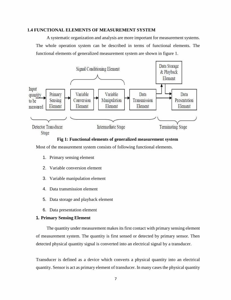
functional elements of generalized measurement system are shown in figure 1.

Fig 1: Functional elements of generalized measurement system

Most of the measurement system consists of following functional elements.

1. Primary sensing element

2. Variable conversion element

3. Variable manipulation element

4. Data transmission element

5. Data storage and playback element

6. Data presentation element

1. Primary Sensing Element

The quantity under measurement makes its first contact with primary sensing element

of measurement system. The quantity is first sensed or detected by primary sensor. Then

detected physical quantity signal is converted into an electrical signal by a transducer.

Transducer is defined as a device which converts a physical quantity into an electrical

quantity. Sensor is act as primary element of transducer. In many cases the physical quantity

8

is directly converted into an electrical quantity by a transducer. So the first stage of a

measurement system is known as a detector transducer stage.

Example, Pressure transducer with pressure sensor, Temperature sensor etc.,

2. Variable Conversion Element

The output of primary sensing element is electrical signal of any form like a voltage,

a frequency or some other electrical parameter. Sometime this output not suitable for next

level of system. So it is necessary to convert the output some other suitable form while

maintaining the original signal to perform the desired function the system.

For example the output primary sensing element is in analog form of signal and next

stage of system accepts only in digital form of signal. So, we have to convert analog signal

into digital form using an A/D converter. Here A/D converter is act as variable conversion

element.

3. Variable Manipulation Element

The function of variable manipulation element is to manipulate the signal offered but

original nature of signal is maintained in same state. Here manipulation means only change

in the numerical value of signal.

Examples,

1. Voltage amplifier is act as variable manipulation element. Voltage amplifier accepts a

small voltage signal as input and produces the voltage with greater magnitude .Here

numerical value of voltage magnitude is increased.

2. Attenuator acts as variable manipulation element. It accepts a high voltage signal and

produces the voltage or power with lower magnitude. Here numerical value of voltage

magnitude is decreased.

o Linear process manipulation elements: Amplification, attenuation, integration,

differentiation, addition and subtraction etc.,

o Nonlinear process manipulation elements: Modulation, detection, sampling,

filtering, chopping and clipping etc.,

All these elements are performed on the signal to bring it to desired level to be accepted by

the next stage of measurement system. This process of conversion is called signal

9

conditioning. The combination of variable conversion and variable manipulation elements

are called as Signal Conditioning Element.

4. Data Transmission Element

The elements of measurement system are actually physically separated; it becomes

necessary to transmit the data from one to another. The element which is performs this

function is called as data transmission element.

Example, Control signals are transmitted from earth station to Space-crafts by a telemetry

system using radio signals. Here telemetry system is act as data transmission element.

The combination of Signal conditioning and transmission element is known as Intermediate

Stage of measurement system.

5. Data storage and playback element

Some applications requires a separate data storage and playback function for easily

rebuild the stored data based on the command. The data storage is made in the form of

pen/ink and digital recording. Examples, magnetic tape recorder/ reproducer, X-Y

recorder, X-t recorder, Optical Disc recording ect.,

6. Data presentation Element

The function of this element in the measurement system is to communicate the

information about the measured physical quantity to human observer or to present it in an

understandable form for monitoring, control and analysis purposes.Visual display devices

are required for monitoring of measured data. These devices may be analog or digital

instruments like ammeter, voltmeter, camera, CRT, printers, analog and digital computers.

Computers are used for control and analysis of measured data of measurement system. This

Final stage of measurement system is known as Terminating stage.

1.41 EXAMPLE OF GENERALIZED MEASUREMENT SYSTEM

Bourdon Tube Pressure Gauge:

The simple pressure measurement system using bourdon tube pressure gauge is shown in

figure 2.The detail functional elements of this pressure measurement system is given below.

Primary sensing element and : Pressure Sensed

Variable conversion element : Bourdon Tube

10

Data Transmission element : Mechanical

Linkages Variable manipulation Element : Gearing

arrangement

Data presentation Element : Pointer and Dial

Fig. 2 Bourdon tube pressure gauge

In this measurement system, bourdon tube is act as primary sensing and variable

conversion element. The input pressure is sensed and converted into small displacement by

a bourdon tube. On account of input pressure the closed end of the tube is displaced.

Because of this pressure in converted into small displacement. The closed end of bourdon

tube is connected through mechanical linkage to a gearing arrangement.

The small displacement signal can be amplified by gearing arrangement and

transmitted by mechanical linkages and finally it makes the pointer to rotate on a large

angle of scale. If it is calibrated with known input pressure, gives the measurement of the

pressure signal applied to the bourdon tube in measurand.

11

2. CHARACTERISTICS OF MEASURING INSTRUMENTS

These performance characteristics of an instrument are very important in their selection.

Static Characteristics: Static characteristics of an instrument are considered for

instruments which are used to measure an unvarying process condition.

Performance criteria based upon static relations represent the static Characteristics.

(The static characteristics are the value or performance given after the steady state

condition has reached).

Dynamic Characteristics: Dynamic characteristics of an instrument are considered

for instruments which are used to measure a varying process condition. Performance

criteria based upon dynamic relations represent the dynamic Characteristics.

2.1 STATIC CHARACTERISTICS

1) Accuracy

Accuracy is defined as the degree of closeness with which an instrument reading

approaches to the true value of the quantity being measured. It determines the closeness to

true value of instrument reading.Accuracy is represented by percentage of full scale reading

or in terms of inaccuracy or in terms of error value.Example, Accuracy of temperature

measuring instrument might be specified by±3ºC. This accuracy means the temperature

reading might be within + or -3ºC deviation from the true value. Accuracy of an instrument

is specified by ±5% for the range of 0 to 200ºC in the

temperature scale means the reading might be within + or -10ºC of the true reading.

2) Precision

Precision is the degree of repeatability of a series of the measurement. Precision is

measures of the degree of closeness of agreement within a group of measurements are

repeatedly made under the prescribed condition. Precision is used in measurements to

describe the stability or reliability or the reproducibility of results.

12

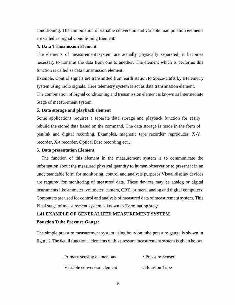
Table1: Comparison between accuracy and precision

Accuracy Precision

It refers to degree of closeness of the

measured value to the true value

It refers to the degree of agreement among

group of readings

Accuracy gives the maximum error that is

maximum departure of the final result from its

true value

Precision of a measuring system gives

its capability to reproduce a certain

reading with a given accuracy

3) Bias

Bias is quantitative term describing the difference between the average of measured

readings made on the same instrument and its true value (It is a characteristic of measuring

instruments to give indications of the value of a measured quantity for which the average

value differs from true value).

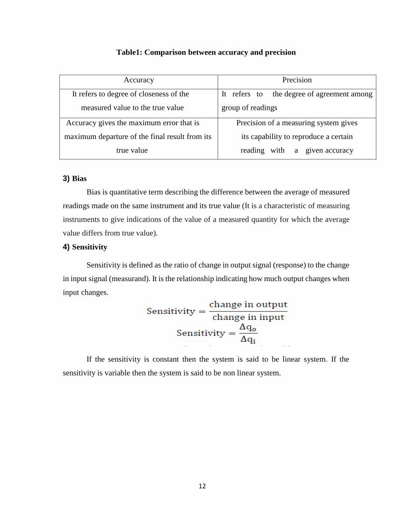
4) Sensitivity

Sensitivity is defined as the ratio of change in output signal (response) to the change

in input signal (measurand). It is the relationship indicating how much output changes when

input changes.

If the sensitivity is constant then the system is said to be linear system. If the

sensitivity is variable then the system is said to be non linear system.

13

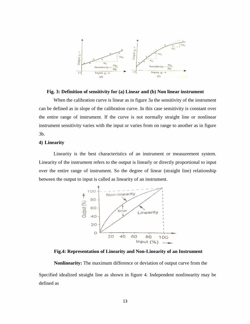
Fig. 3: Definition of sensitivity for (a) Linear and (b) Non linear instrument

When the calibration curve is linear as in figure 3a the sensitivity of the instrument

can be defined as in slope of the calibration curve. In this case sensitivity is constant over

the entire range of instrument. If the curve is not normally straight line or nonlinear

instrument sensitivity varies with the input or varies from on range to another as in figure

3b.

4) Linearity

Linearity is the best characteristics of an instrument or measurement system.

Linearity of the instrument refers to the output is linearly or directly proportional to input

over the entire range of instrument. So the degree of linear (straight line) relationship

between the output to input is called as linearity of an instrument.

Fig.4: Representation of Linearity and Non-Linearity of an Instrument

Nonlinearity: The maximum difference or deviation of output curve from the

Specified idealized straight line as shown in figure 4. Independent nonlinearity may be

defined as

14

5) Resolution

Resolution or Discrimination is the smallest change in the input value that is

required to cause an appreciable change in the output. (The smallest increment in input or

input change which can be detected by an instrument is called as resolution or

discrimination)

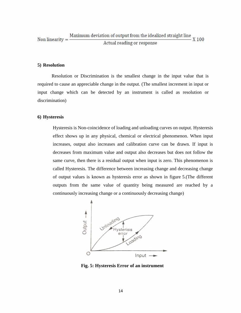
6) Hysteresis

Hysteresis is Non-coincidence of loading and unloading curves on output. Hysteresis

effect shows up in any physical, chemical or electrical phenomenon. When input

increases, output also increases and calibration curve can be drawn. If input is

decreases from maximum value and output also decreases but does not follow the

same curve, then there is a residual output when input is zero. This phenomenon is

called Hysteresis. The difference between increasing change and decreasing change

of output values is known as hysteresis error as shown in figure 5.(The different

outputs from the same value of quantity being measured are reached by a

continuously increasing change or a continuously decreasing change)

Fig. 5: Hysteresis Error of an instrument

15

7) Dead Zone

Dead zone or dead band is defined as the largest change of input quantity for which

there is no output the instrument due the factors such as friction, backlash and hysteresis

within the system. (The region upto which the instrument does not respond for an input

change is called dead zone).Dead time is the time required by an instrument to begin to

respond to change in input quantity.

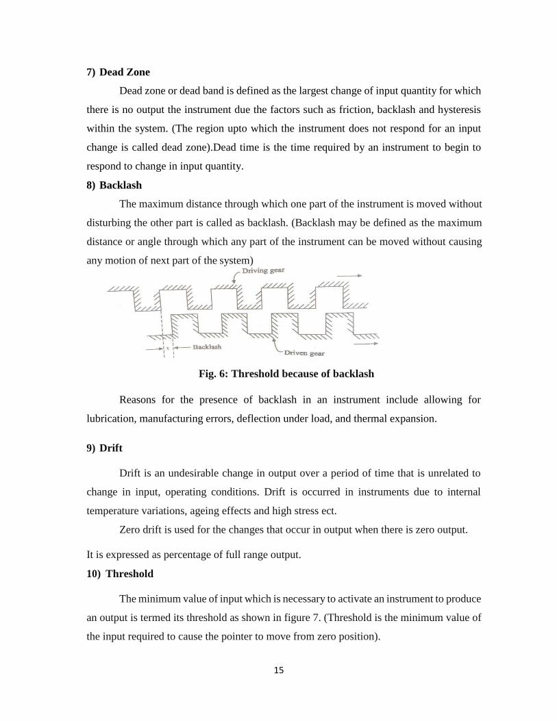
8) Backlash

The maximum distance through which one part of the instrument is moved without

disturbing the other part is called as backlash. (Backlash may be defined as the maximum

distance or angle through which any part of the instrument can be moved without causing

any motion of next part of the system)

Fig. 6: Threshold because of backlash

Reasons for the presence of backlash in an instrument include allowing for

lubrication, manufacturing errors, deflection under load, and thermal expansion.

9) Drift

Drift is an undesirable change in output over a period of time that is unrelated to

change in input, operating conditions. Drift is occurred in instruments due to internal

temperature variations, ageing effects and high stress ect.

Zero drift is used for the changes that occur in output when there is zero output.

It is expressed as percentage of full range output.

10) Threshold

The minimum value of input which is necessary to activate an instrument to produce

an output is termed its threshold as shown in figure 7. (Threshold is the minimum value of

the input required to cause the pointer to move from zero position).

16

Fig. 7 Threshold effect

11) Input Impedance

The magnitude of the impedance of element connected across the signal source is

called Input Impedance. Figure 8 shows a voltage signal source and input device connected

across it.

Fig. 8 voltage source and input device

The magnitude of the input impedance is given by

Power extracted by the input device from the signal source is

From above two expressions it is clear that a low input impedance device connected across the

voltage signal source draws more current and more power from signal source than high input

impedance device.

17

12) Loading Effect

Loading effect is the incapability of the system to faith fully measure, record or

control the input signal in accurate form.

13) Repeatability

Repeatability is defined as the ability of an instrument to give the same output for

repeated applications of same input value under same environmental condition.

14) Reproducibility

Reproducibility is defined as the ability of an instrument to reproduce the same

output for repeated applications of same input value under different environment

condition. In case of perfect reproducibility the instrument satisfies no drift condition.

15) Static Error

The difference between the measured value of quantity and true value (Reference

Value) of quantity is called as Error.

Error = Measured value - True

Value δA= Am - At

δA - error

Am - Measured value of

quantity At - True value of

quantity

16) Static Correction

It is the difference between the true value and the measurement value of the quantity

δC= At – Am = - δA

δC – Static correction

17) Scale Range

It can be defined as the measure of the instrument between the lowest and

highest readings it can measure. A thermometer has a scale from −40°C to 100°C.

Thus the range varies from −40°C to 100°C.

18

18) Scale Span

It can be defined as the range of an instrument from the minimum to maximum scale

value. In the case of a thermometer, its scale goes from −40°C to 100°C. Thus its span is

140°C. As said before accuracy is defined as a percentage of span. It is actually a

deviation from true expressed as a percentage of the span.

2.2 DYNAMIC CHARACTERISTICS

The dynamic behaviour of an instrument is determined by applying some standard

form of known and predetermined input to its primary element (sensing element) and then

studies the output. Generally dynamic behaviour is determined by

applying following three types of inputs.

1. Step Input: Step change in which the primary element is subjected to an

instantaneous and finite change in measured variable.

2. Linear Input: Linear change, in which the primary element is, follows a measured

variable, changing linearly with time.

3. Sinusoidal input: Sinusoidal change, in which the primary element follows a

measured variable, the magnitude of which changes in accordance with a sinusoidal

function of constant amplitude.

The dynamic characteristics of an instrument are

(i) Speed of response

(ii) Fidelity

(iii) Lag

(iv) Dynamic error

(i) Speed of Response

It is the rapidity with which an instrument responds to changes in the measured

quantity.

(ii) Fidelity

It is the degree to which an instrument indicates the changes in the measured

variable without dynamic error (faithful reproduction or fidelity of an instrument is the

ability of reproducing an input signal faithfully (truly).

19

(iii) Lag

It is the retardation or delay in the response of an instrument to changes in the

measured variable. The measuring lags are two types:

Retardation type: In this case the response of an instrument begins immediately

after a change in measured variable is occurred.

Time delay type: In this case the response of an instrument begins after a dead

time after the application of the input quantity.

(iv) Dynamic Error

Error which is caused by dynamic influences acting on the system such as vibration, roll,

pitch or linear acceleration. This error may have an amplitude and usually a frequency

related to the environmental influences and the parameters of the system itself.

3. CLASSIFICATION OF ERRORS

All measurement can be made without perfect accuracy (degree of error must

always be assumed). In reality, no measurement can ever made with 100% accuracy. It is

important to find that actual accuracy and different types of errors can be occurred in

measuring instruments. Errors may arise from different sources and usually classified as

follows, Classification of Error

1. Gross Errors

2. Systematic Errors

a) Instrumental errors

i) Inherent shortcomings of instruments

ii) Misuse of instruments

iii) Loading effects

b) Environmental errors

c) Observational errors

20

3. Random Errors

1. Gross Errors

The main source of Gross errors is human mistakes in reading or using instruments

and in recording and calculating measured quantity. As long as human beings are involved

and they may grossly misread the scale reading, then definitely some gross errors will be

occurred in measured value.

Example, Due to an oversight, Experimenter may read the temperature as 22.7oC

while the actual reading may be 32.7oC He may transpose the reading while recording. For

example, he may read 16.7oC and record 27.6oC as an alternative.

The complete elimination of gross errors is maybe impossible, one should try to

predict and correct them. Some gross errors are easily identified while others may be very

difficult to detect. Gross errors can be avoided by using the following two ways.

Great care should be taken in reading and recording the data.

Two, three or even more readings should be taken for the quantity being measured

by using different experimenters and different reading point (different environment

condition of instrument) to avoid re-reading with same error. So it is suitable to take a large

number of readings as a close agreement between readings assures that no gross error has

been occurred in measured values.

2. Systematic Errors

Systematic errors are divided into following three categories.

i. Instrumental Errors

ii. Environmental Errors

iii. Observational Errors

i) Instrumental Errors

These errors are arises due to following three reasons (sources of error).

a) Due to inherent shortcoming of instrument

b) Due to misuse of the instruments, and

c) Due to loading effects of instruments

21

a) Inherent Shortcomings of instruments

These errors are inherent in instruments because of their mechanical structure due

to construction, calibration or operation of the instruments or measuring devices.These

errors may cause the instrument to read too low or too high.Example, if the spring (used

for producing controlling torque) of a permanent magnet instrument has become weak, so

the instrument will always read high.Errors may be caused because of friction, hysteresis

or even gear backlash.

Elimination or reduction methods of these errors,

o The instrument may be re-calibrated carefully.

o The procedure of measurement must be carefully planned. Substitution

methods or calibration against standards may be used for the purpose.

o Correction factors should be applied after determining the instrumental

errors.

b) Misuse of Instruments

In some cases the errors are occurred in measurement due to the fault of the operator

than that of the instrument. A good instrument used in an unintelligent way may give wrong

results.

Examples, Misuse of instruments may be failure to do zero adjustment of

instrument, poor initial adjustments, using leads of too high a resistance and ill practices of

instrument beyond the manufacturer’s instruction and specifications ect.

c) Loading Effects

The errors committed by loading effects due to improper use of an instrument for

measurement work. In measurement system, loading effects are identified and corrections

should be made or more suitable instruments can be used.

Example, a well calibrated voltmeter may give a misleading (may be false) voltage

reading when connected across a high resistance circuit. The same voltmeter, when

connected across a low resistance circuit may give a more reliable reading (dependable or

22

steady or true value).In this example, voltmeter has a loading effect on the circuit, altering

the actual circuit conditions by measurement process. So errors caused by loading effect of

the meters can be avoided by using them intelligently.

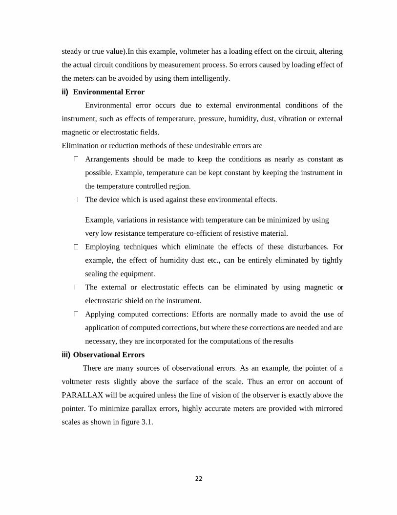
ii) Environmental Error

Environmental error occurs due to external environmental conditions of the

instrument, such as effects of temperature, pressure, humidity, dust, vibration or external

magnetic or electrostatic fields.

Elimination or reduction methods of these undesirable errors are

Arrangements should be made to keep the conditions as nearly as constant as

possible. Example, temperature can be kept constant by keeping the instrument in

the temperature controlled region.

The device which is used against these environmental effects.

Example, variations in resistance with temperature can be minimized by using

very low resistance temperature co-efficient of resistive material.

Employing techniques which eliminate the effects of these disturbances. For

example, the effect of humidity dust etc., can be entirely eliminated by tightly

sealing the equipment.

The external or electrostatic effects can be eliminated by using magnetic or

electrostatic shield on the instrument.

Applying computed corrections: Efforts are normally made to avoid the use of

application of computed corrections, but where these corrections are needed and are

necessary, they are incorporated for the computations of the results

iii) Observational Errors

There are many sources of observational errors. As an example, the pointer of a

voltmeter rests slightly above the surface of the scale. Thus an error on account of

PARALLAX will be acquired unless the line of vision of the observer is exactly above the

pointer. To minimize parallax errors, highly accurate meters are provided with mirrored

scales as shown in figure 3.1.

23

Fig. 9: Errors due to parallax

When the pointer’s image appears hidden by the pointer, observer’s eye is directly in line

with the pointer. Although a mirrored scale minimizes parallax error,

Fig.10: Arrangements showing scale and pointer in the same plane

The observational errors are also occurs due to involvement of human factors. For example,

there are observational errors in measurements involving timing of an event Different

observer may produce different results, especially when sound and light measurement are

involved. The complete elimination of this error can be achieved by using digital display

of output.

3. Random Errors

These errors are occurred due to unknown causes and are observed when the magnitude

and polarity of a measurement fluctuate in changeable (random) manner.The quantity being

measure is affected by many happenings or disturbances and ambient influence about

which we are unaware are lumped together and called as Random or Residual. The errors

24

caused by these disturbances are called Random Errors. Since the errors remain even after

the systematic errors have been taken care, those errors are called as Residual (Random)

Errors.Random errors cannot normally be predicted or corrected, but they can be

minimized by skilled observer and using a well maintained quality instrument.

4.1 SOURCES OF ERRORS

The sources of error, other than the inability of a piece of hardware to provide a

true measurement are listed below,

1) Insufficient knowledge of process parameters and design conditions.

2) Poor design

3) Change in process parameters, irregularities, upsets (disturbances) ect.

4) Poor maintenance

5) Errors caused by people who operate the instrument or equipment.

Certain design limitations.

Errors in Measuring Instruments

No measurement is free from error in reality. An intelligent skill in taking

measurements is the ability to understand results in terms of possible errors. If the

precision of the instrument is sufficient, no matter what its accuracy is, a difference will

always be observed between two measured results. So an understanding and careful

evaluation of the errors is necessary in measuring instruments. The Accuracy of an

instrument is measured in terms of errors.

True value

The true value of quantity being measured is defined as the average of an infinite

number of measured values when the average deviation due to the various contributing

factors tends to zero.In ideal situation is not possible to determine the True value of a

quantity by experimental way. Normally an experimenter would never know that the

quantity being measured by experimental way is the True value of the quantity or not.In

practice the true value would be determined by a “standard method”, that is a method

agreed by experts with sufficient accurate.

25

Static Error

Static error is defined as a difference between the measured value and the true value

of the quantity being measured. It is expressed as follows.

δA= Am - At ------------------------ (1)

Where, δA= Error, Am =Measured value of quantity and At= True value of

quantity. δA is also called as absolute static error of quantity A and it is expressed as

follows.

ε0=δA (2)

Where, ε0 = Absolute static error of quantity A under measurement.

The absolute value of δA does not specify exactly the accuracy of measurement

.so the quality of measurement is provided by relative static error.

Relative static error

Relative static error is defined as the ratio between the absolute static errors and

true value of quantity being measured. It is expressed as follows.

26

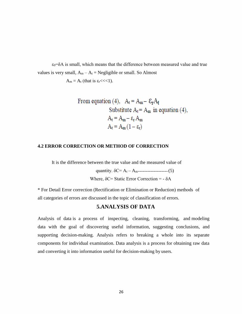
ε0=δA is small, which means that the difference between measured value and true

values is very small, Am – At = Negligible or small. So Almost

Am = At (that is εr<<<1).

4.2 ERROR CORRECTION OR METHOD OF CORRECTION

It is the difference between the true value and the measured value of

quantity. δC= At – Am ------------------- (5)

Where, δC= Static Error Correction = - δA

* For Detail Error correction (Rectification or Elimination or Reduction) methods of

all categories of errors are discussed in the topic of classification of errors.

5.ANALYSIS OF DATA

Analysis of data is a process of inspecting, cleaning, transforming, and modeling

data with the goal of discovering useful information, suggesting conclusions, and

supporting decision-making. Analysis refers to breaking a whole into its separate

components for individual examination. Data analysis is a process for obtaining raw data

and converting it into information useful for decision-making by users.

27

STATISTICAL EVALUATION OF MEASUREMENT DATA

Statistical Evaluation of measured data is obtained in two methods of tests as shown

in below.

Multi Sample Test: In multi sample test, repeated measured data have been

acquired by different instruments, different methods of measurement and

different observer.

Single Sample Test: measured data have been acquired by identical conditions

(same

instrument, methods and observer) at different times.

Statistical Evaluation methods will give the most probable true value of measured quantity.

The mathematical background statistical evaluation methods are Arithmetic Mean,

Deviation Average Deviation, Standard Deviation and variance.

Arithmetic Mean

The most probable value of measured reading is the arithmetic mean of the number

of reading taken. The best approximation is made when the number of readings of the same

quantity is very large. Arithmetic mean or average of measured variables X

is calculated by taking the sum of all readings and dividing by the number of reading.

The Average is given by,

Where, X= Arithmetic mean, x1, x2....... xn = Readings or variable or samples and n=

number of readings.

Deviation (Deviation from the Average value)

The Deviation is departure of the observed reading from the arithmetic mean

of the group of reading. Let the deviation of reading x1 be d1 and that of x2 be d2 etc.,

Average Deviation:

Average deviation defined as the average of the modulus (without respect to its sign)

of the individual deviations and is given by,

Where, D= Average Deviation.

28

The average deviation is used to identify precision of the instruments which is used

in making measurements. Highly precise instruments will give a low average deviation

between readings.

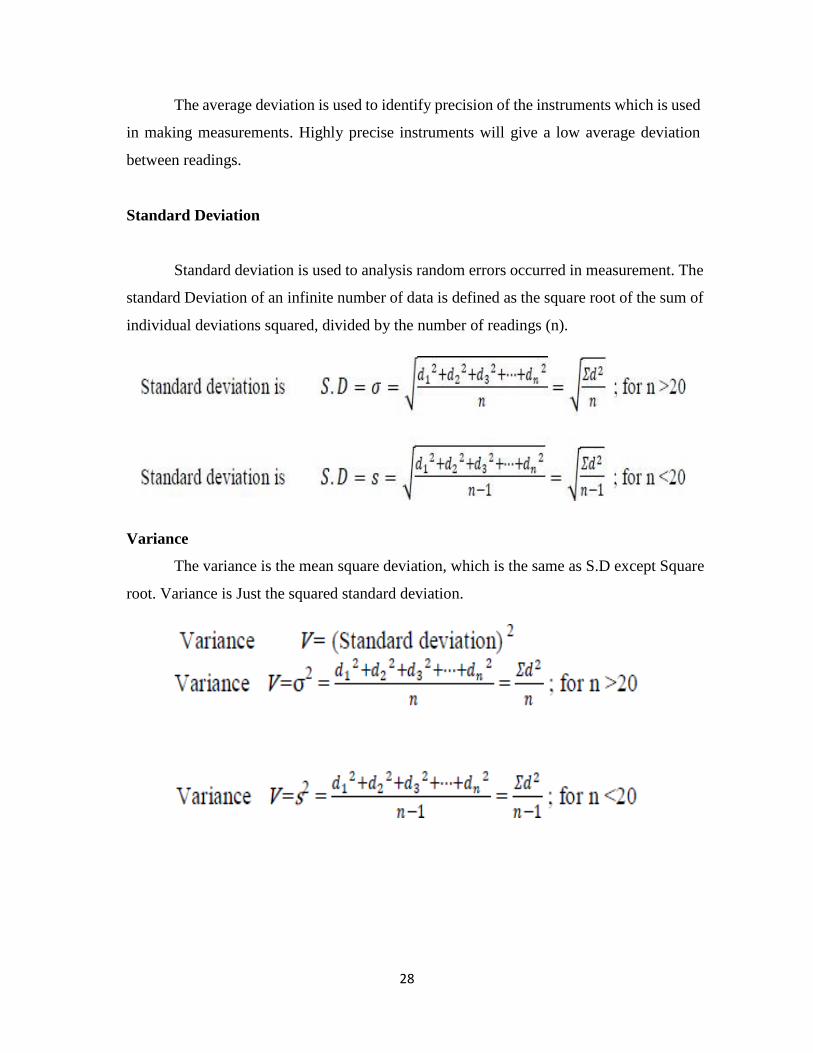
Standard Deviation

Standard deviation is used to analysis random errors occurred in measurement. The

standard Deviation of an infinite number of data is defined as the square root of the sum of

individual deviations squared, divided by the number of readings (n).

Variance

The variance is the mean square deviation, which is the same as S.D except Square

root. Variance is Just the squared standard deviation.

29

Histogram:

When a number of Multisample observations are taken experimentally there is

a scatter of the data about some central value. For representing this results in the form

of a Histogram. A histogram is also called a frequency distribution curve.

Example: Following table3.1 shows a set of 50 readings of length measurement. The

most probable or central value of length is 100mm represented as shown.

Table 2:Sample Reading

Length (mm)

Number of observed

readings

(frequency or occurrence)

99.7 1

99.8 4

99.9 12

100.0 19

100.1 10

100.2 3

100.3 1

Total number of readings =50

Fig. 11: Histogram

This histogram indicates the number of occurrence of particular value. At the

central value of 100mm is occurred 19 times and recorded to the nearest 0.1mm as shown

in figure 3.3. Here bell shape dotted line curve is called as normal or Gaussian curve.

30

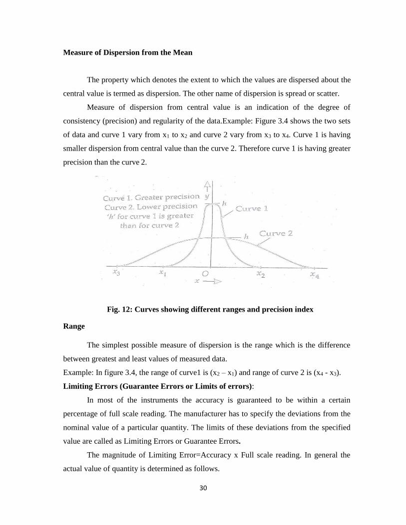
Measure of Dispersion from the Mean

The property which denotes the extent to which the values are dispersed about the

central value is termed as dispersion. The other name of dispersion is spread or scatter.

Measure of dispersion from central value is an indication of the degree of

consistency (precision) and regularity of the data.Example: Figure 3.4 shows the two sets

of data and curve 1 vary from x1 to x2 and curve 2 vary from x3 to x4. Curve 1 is having

smaller dispersion from central value than the curve 2. Therefore curve 1 is having greater

precision than the curve 2.

Fig. 12: Curves showing different ranges and precision index

Range

The simplest possible measure of dispersion is the range which is the difference

between greatest and least values of measured data.

Example: In figure 3.4, the range of curve1 is (x2 – x1) and range of curve 2 is (x4 - x3).

Limiting Errors (Guarantee Errors or Limits of errors):

In most of the instruments the accuracy is guaranteed to be within a certain

percentage of full scale reading. The manufacturer has to specify the deviations from the

nominal value of a particular quantity. The limits of these deviations from the specified

value are called as Limiting Errors or Guarantee Errors.

The magnitude of Limiting Error=Accuracy x Full scale reading. In general the

actual value of quantity is determined as follows.

31

Actual Value of Quantity = Nominal value ± Limiting Error

Aa = An ± δA

Where, Aa = Actual value of quantity; An = Nominal value of Quantity; ± δA= Limiting

error.

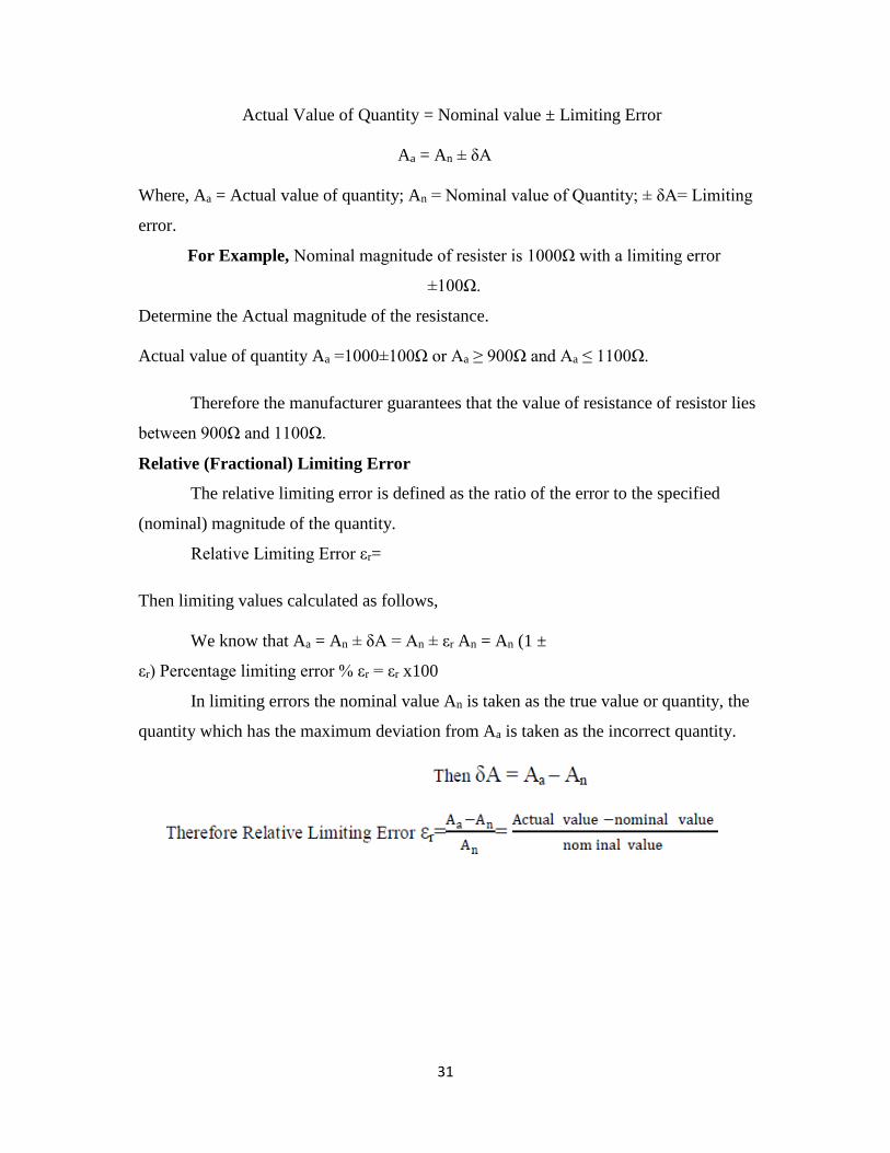
For Example, Nominal magnitude of resister is 1000Ω with a limiting error

±100Ω.

Determine the Actual magnitude of the resistance.

Actual value of quantity Aa =1000±100Ω or Aa ≥ 900Ω and Aa ≤ 1100Ω.

Therefore the manufacturer guarantees that the value of resistance of resistor lies

between 900Ω and 1100Ω.

Relative (Fractional) Limiting Error

The relative limiting error is defined as the ratio of the error to the specified

(nominal) magnitude of the quantity.

Relative Limiting Error εr=

Then limiting values calculated as follows,

We know that Aa = An ± δA = An ± εr An = An (1 ±

εr) Percentage limiting error % εr = εr x100

In limiting errors the nominal value An is taken as the true value or quantity, the

quantity which has the maximum deviation from Aa is taken as the incorrect quantity.

32

Probable error

The most probable or best value of a Gaussian distribution is obtained by taking

arithmetic mean of the various values of the variety. A convenient measure of precision is

achieved by the quantity r. It is called Probable Error of P.E. It is expressed as follows,

Probable Error = P. E = r = 0.4769

h

Where r= probable error and h= constant called precision index

Gaussian distribution and Histogram are used to estimate the probable error of any

measurement.

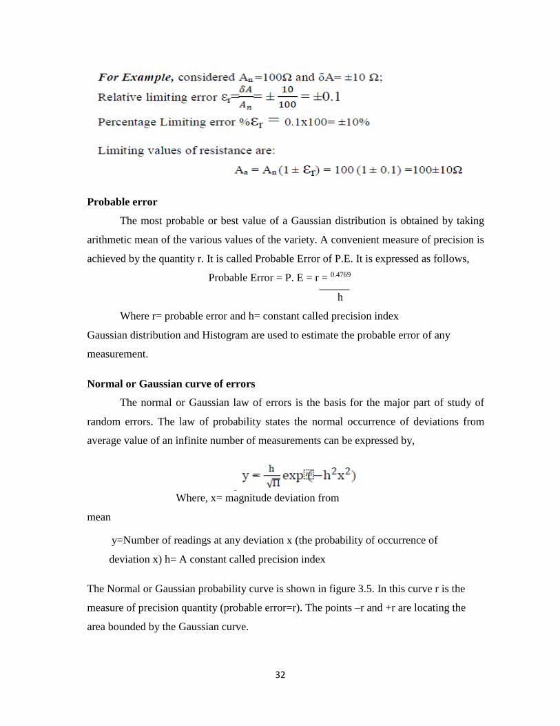
Normal or Gaussian curve of errors

The normal or Gaussian law of errors is the basis for the major part of study of

random errors. The law of probability states the normal occurrence of deviations from

average value of an infinite number of measurements can be expressed by,

Where, x= magnitude deviation from

mean

y=Number of readings at any deviation x (the probability of occurrence of

deviation x) h= A constant called precision index

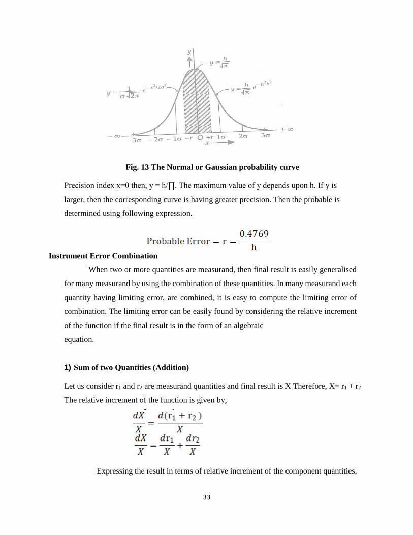
The Normal or Gaussian probability curve is shown in figure 3.5. In this curve r is the

measure of precision quantity (probable error=r). The points –r and +r are locating the

area bounded by the Gaussian curve.

33

Fig. 13 The Normal or Gaussian probability curve

Precision index x=0 then, y = h/∏. The maximum value of y depends upon h. If y is

larger, then the corresponding curve is having greater precision. Then the probable is

determined using following expression.

Instrument Error Combination

When two or more quantities are measurand, then final result is easily generalised

for many measurand by using the combination of these quantities. In many measurand each

quantity having limiting error, are combined, it is easy to compute the limiting error of

combination. The limiting error can be easily found by considering the relative increment

of the function if the final result is in the form of an algebraic

equation.

1) Sum of two Quantities (Addition)

Let us consider r1 and r2 are measurand quantities and final result is X Therefore, X= r1 + r2

The relative increment of the function is given by,

Expressing the result in terms of relative increment of the component quantities,

34

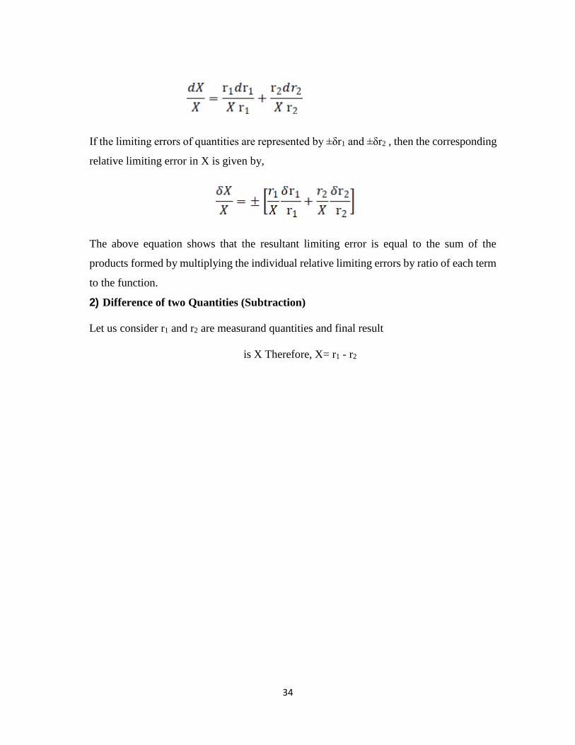
If the limiting errors of quantities are represented by ±δr1 and ±δr2 , then the corresponding

relative limiting error in X is given by,

The above equation shows that the resultant limiting error is equal to the sum of the

products formed by multiplying the individual relative limiting errors by ratio of each term

to the function.

2) Difference of two Quantities (Subtraction)

Let us consider r1 and r2 are measurand quantities and final result

is X Therefore, X= r1 - r2

35

Therefore the relative limiting error of product of terms is equal to the smn of relative

limiting errors of terrors.

36

Calibration

Calibration is the process of checking the accuracy of instrument by comparing

the instrument reading with a standard or against a similar meter of known accuracy. So

using calibration is used to find the errors and accuracy of the measurement system or an

instrument.

Calibration is an essential process to be undertaken for each instrument and

measuring system regularly. The instruments which are actually used for measurement

work must be calibrated against some reference instruments in which is having higher

accuracy. Reference instruments must be calibrated against instrument of still higher

accuracy or against primary standard or against other standards of known accuracy.

The calibration is better carried out under the predetermined environmental

conditions. All industrial grade instruments can be checked for accuracy in the laboratory

37

by using the working standard.Certification of an instrument manufactured by an industry

is undertaken by National Physical Laboratory and other authorizes laboratories where the

secondary standards and working standards are kept.

Process of Calibration

The procedure involved in calibration is called as process of calibration. Calibration

procedure involves the comparison of particular instrument with either

A primary standard,

A secondary standard with higher accuracy than the instrument to be calibrated

An instrument of known accuracy.

Procedure of calibration as follows.

Study the construction of the instrument and identify and list all the possible

inputs.

Choose, as best as one can, which of the inputs will be significant in the

application for which the instrument is to be calibrated.

Standard and secure apparatus that will allow all significant inputs to vary over

the ranges considered necessary.

By holding some input constant, varying others and recording the output, develop

the desired static input-output relations.

Theory and Principles of Calibration Methods

Calibration methods are classified into following two types,

1) Primary or Absolute method of calibration

2) Secondary or Comparison method of calibration

i. Direct comparison method of calibration

ii. Indirect comparison method of calibration

38

1) Primary or Absolute method of calibration

If the particular test instrument (the instrument to be calibrated) is calibrated against

primary standard, then the calibration is called as primary or absolute calibration. After the

primary calibration, the instrument can be used as a secondary calibration instrument.

2) Secondary or Comparison calibration method

If the instrument is calibrated against secondary standard instrument, then the

calibration is called as secondary calibration. This method is used for further calibration of

other devices of lesser accuracy. Secondary calibration instruments are used in laboratory

practice and also in the industries because they are practical calibration sources.

i) Direct comparison method of Calibration

Direct comparison method of calibration with a known input source with same order

of accuracy as primary calibration. So the instrument which is calibrated directly is also

used as secondary calibration instruments.

ii) Indirect comparison method of Calibration

The procedure of indirect method of calibration is based on the equivalence of

two different devices with same comparison concept.

Standards of measurement:

A standard is a physical representation of a unit of measurement. A known accurate

measure of physical quantity is termed as standard. These standards are used to determine

the accuracy of other physical quantities by the comparison method.

Example, the fundamental unit of mass in the International System is the Kilogram

and defined as the mass of a cubic decimetre of water at its temperature of maximum of

density of 4oC.

Different standards are developed for checking the other units of measurements

39

and all these standards are preserved at the International Bureau of Weight and

Measures at Serves, Paris.

Classification of Standards

Standards are classified into four types, based on the functions and applications.

1) International standards

2) Primary standards

3) Secondary standards

4) Working standards

1) International Standard

International standards are defined and established upon internationally. They

are maintained at the International Bureau of Weights and measures and are not

accessible to ordinary users for measurements and calibration. They are periodically

evaluated and checked by absolute measurements in terms of fundamental units of

physics.

International Ohms It is defined as the resistance offered by a column of

mercury having a mass of 14.4521gms, uniform cross sectional area and length

of 106.300cm, to the flow of constant current at the melting point of ice.

2) Primary Standards

Primary standards are maintained by the National Standards Laboratories (NSL)

in different parts of the world.

The principle function of primary standards is the calibration and verification of

secondary standards.

They are not available outside the National Laboratory for calibration.

These primary standards are absolute standards of high accuracy that can be

used as ultimate reference standards.

40

Secondary Standards

These standards are basic reference standards used in industrial laboratories for calibration

of instruments. Each industry has its own secondary standard and maintained by same

industry. Each laboratory periodically sends its secondary standard to the NSL for calibration

and comparison against the primary standards. Certification of measuring accuracy is given

by NSL in terms of primary standards.

4.Working Standards

The working standards are used for day-to-day use in measurement laboratories. So this

standard is the primary tool of a measurement laboratory.These standards may be lower in

accuracy in comparison with secondary standard. It is used to check and calibrate laboratory

instruments for accuracy and performance.

Example, a standard resister for checking of resistance value manufactured.

Reference books

1. Sawhney A.K., “A Course in Electrical, Electronic measurement &

Instrumentation”, Dhanpat Rai & sons, 18th Edition, Reprint 2010.

2. Doebelin E.O., “Measurement System Applications and Design”, McGraw Hill,

5th Edition, 2004.

3. Jain R.K., “Mechanical and Industrial Measurements”, Khanna Publishers, 11th

edition, Reprint 2005.

4. Jones’ Instrument Technology, Instrumentation Systems, Edited by B.E.Noltingk,

Vol 4, 4th edition, ELBS, 1987.

5. Murthy D.V.S., “Transducers and Instrumentation”, Printice Hall of India, 13th

printing, 2006.

6. Gnanavadivel,“Measurements and Instrumentation”,Anuradha Publication, Second

Revised Edition 2011.

1

SCHOOL OF ELECTRICAL AND ELECTRONICS

DEPARTMENT OF ELECTRICAL AND ELECTRONICS

UNIT – II

MEASUREMENT AND INSTRUMENTATION – SIC 1203

2

UNIT 2 ELECTRICAL MEASUREMENTS

Units of voltage and current - principle of operation of D’Arsonval Galvanometer -

principle, operation, constructional details and comparison of the following: permanent

magnet moving coil, permanent magnet moving iron, Dynamometer, Induction, thermal

and rectifier type instruments, Power measurement - Voltmeter ammeter method,

Ammeter voltmeter method, Electro-dynamic wattmeter - Low power factor wattmeter

Current

Current is the rate at which electric charge flows past a point in a circuit. Symbol is I and unit

is A or amps

Voltage

Voltage is the electrical force that would drive an electric current between two points. And

symbol is v units is volts or voltage

1. PRINCIPLE OF D’ARSONVAL GALVANOMETER

An action caused by electromagnetic deflection, using a coil of wire and a magnetized field.

When current passes through the coil, a needle is deflected. Whenever electrons flow through

a conductor, a magnetic field proportional to the current is created. This effect is useful for

measuring current and is employed in many practical meters.

Moving Coil:

It is the current carrying element. It is either rectangular or circular in shape and consists of

number of turns of fine wire. This coil is suspended so that it is free to turn about its vertical

axis of symmetry. It is arranged in a uniform, radial, horizontal magnetic field in the air gap

between pole pieces of a permanent magnet and iron core. The iron core is spherical in shape if

the coil is circular but is cylindrical if the coil is rectangular. The iron core is used to provide a

flux path of low reluctance and therefore to provide strong magnetic field for the coil to move

in. this increases the deflecting torque and hence the sensitivity of the galvanometer. The

length of air gap is about

3

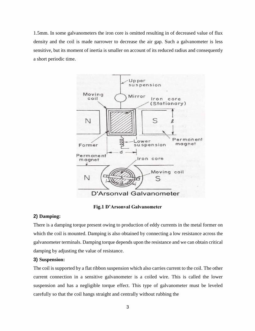
1.5mm. In some galvanometers the iron core is omitted resulting in of decreased value of flux

density and the coil is made narrower to decrease the air gap. Such a galvanometer is less

sensitive, but its moment of inertia is smaller on account of its reduced radius and consequently

a short periodic time.

Fig.1 D’Arsonval Galvanometer

2) Damping:

There is a damping torque present owing to production of eddy currents in the metal former on

which the coil is mounted. Damping is also obtained by connecting a low resistance across the

galvanometer terminals. Damping torque depends upon the resistance and we can obtain critical

damping by adjusting the value of resistance.

3) Suspension:

The coil is supported by a flat ribbon suspension which also carries current to the coil. The other

current connection in a sensitive galvanometer is a coiled wire. This is called the lower

suspension and has a negligible torque effect. This type of galvanometer must be leveled

carefully so that the coil hangs straight and centrally without rubbing the

4

poles or the soft iron cylinder. Some portable galvanometers which do not require exact leveling

have ” taut suspensions” consisting of straight flat strips kept under tension for at the both top

and at the bottom.

The upper suspension consists of gold or copper wire of nearly 0.012-5 or 0.02-5 mm diameter

rolled into the form of a ribbon. This is not very strong mechanically; so that the galvanometers

must he handled carefully without jerks. Sensitive galvanometers are provided with coil clamps

to the strain from suspension, while the galvanometer is being moved.

4) Indication:

The suspension carries a small mirror upon which a beam of light is cast. The beam of light is

reflected on a scale upon which the deflection is measured. This scale is usually about 1 meter

away from the instrument, although ½ meter may be used for greater compactness.

5) Zero Setting:

A torsion head is provided for adjusting the position of the coil and also for zero setting.

Operation

When a current flows through the coil, the coil generates a magnetic field. This field acts against

the permanent magnet. The coil twists, pushing against the spring, and moves the pointer. The

hand points at a scale indicating the electric current. Careful design of the pole pieces ensures

that the magnetic field is uniform, so that the angular deflection of the pointer is proportional

to the current. A useful meter generally contains provision for damping the mechanical

resonance of the moving coil and pointer, so that the pointer settles quickly to its position

without oscillation

5

2. PERMANENT MAGNET MOVING COIL INSTRUMENT

Principle of moving coil instrument

Moving coil instrument depends on the principle that when a current carrying conductor is

placed on a magnetic field, mechanical force acts on the conductor. The coil placed on the

magnetic field and carrying operating current is attached to the moving system. With the

movement of the coil the pointer moves over the scale.

Fig.2 Permanent magnet moving coil

Construction of PMMC instrument

Moving coil instrument consists of a powerful permanent magnet with soft iron pieces and light

rectangular coil of many turns of fine wire wound on aluminum former inside which is an iron

core as shown in the figure. As it uses permanent magnets they are called “Permanent magnet

moving coil instrument“. The purpose of the coil is to make the field uniform. The coil is

mounted on the spindle and acts as the moving element. The current is led into and out of the

coil by means of the two control hair

6

springs, one above and the other below the coil. The springs also provides the controlling

torque. damping torque is provide by eddy current damping.

Working of PMMC instrument

when the moving coil instrument is connected in the circuit, operating current flows through

the coil. This current carrying coil is placed in the magnetic field produced by the permanent

magnet and therefore, mechanical force acts on the coil. As the coil attached to the moving

system, the pointer moves over the scale. It may be noted here that if current direction is

reversed the torque will also be reversed since the direction of the field of permanent magnet is

same. Hence, the pointer will move in the opposite direction, i.e it will go on the wrong side of

zero. In other words, these instruments work only when current in the circuit is passed in a

definite direction i.e. for d.c only. So it is called permanent magnet moving coil instruments

because a coil moves in the field of a permanent magnet.

Torque Equation for PMMC

The equation for the developed torque of the PMMC can be obtained from the basic law of

electromagnetic torque.

The deflecting torque is given by,

Td = NBAI

Where, Td = deflecting torque in N-m

B = flux density in air gap, Wb/m2

N = Number of turns of the

coils A = effective area of coil

m2

I = current in the moving coil, amperes

Therefore, Td = GI

Where, G = NBA = constant

The controlling torque is provided by the springs and is proportional to the angular deflection

of the pointer.

Tc = KØ

Where, Tc = Controlling Torque

K = Spring Constant Nm/rad or Nm/deg

Ø = angular deflection

7

For the final steady state position,

Td = Tc

Therefore GI = KØ

So, Ø = (G/K)I or I = (K/G) Ø

Thus the deflection is directly proportional to the current passing through the coil. The pointer

deflection can therefore be used to measure current.

Advantage of PMMC instrument

1. Uniform scale.

2. Very effective eddy current damping

3. Power consumption is low.

4. No hysteresis loss.

5. They are not affected by stray field.

6. Require small operating current.

7. Accurate and reliable.

Disadvantage of PMMC instrument

1. Only used for D.C measurement.

2. Costlier compared to moving iron instrument.

3. Some errors are caused due to the aging of the control springs and the permanent

magnets.

3. MOVING IRON INSTRUMENT

There are classified in to two type

1. Attraction type moving iron instrument

2. Repulsion type moving iron instrument

Attraction type moving iron instrument

Principle of attraction type moving iron instrument

An “attraction type” moving-iron instrument consists of a coil, through which the test current

is passed, and a pivoted soft-iron mass attached to the pointer. The resulting magnetic polarity

at the end of the coil nearest the iron mass then induces the opposite magnetic polarity into the

part of the iron mass nearest the coil, which is then drawn by attraction towards the coil,

deflecting the pointer across a scale.

The coil is flat and has a narrow slot like opening. The moving iron is a flat disc or a sector

8

eccentrically mounted. · When the current flows through the coil, a magnetic field is produced

and the moving iron moves from the weaker field outside the coil to the stronger field inside it

or in other words the moving iron is attracted in. · The controlling torque is provide by springs

hut gravity control can be used for panel type of instruments which are vertically mounted. ·

Damping is provided by air friction with the help of a light aluminium piston (attached to the

moving system) which move in a fixed

Fig.3 Attractive moving iron Instrument

chamber closed at one end as shown in Fig. or with the help of a vane (attached to the moving

system) which moves in a fixed sector shaped chamber a shown.

Operation

The current to be measured is passed through the fixed coil. As the current is flow through the

fixed coil, a magnetic field is produced. By magnetic induction the moving iron gets

magnetized. The north pole of moving coil is attracted by the south pole of fixed coil. Thus the

deflecting force is produced due to force of attraction. Since the moving iron is attached with

the spindle, the spindle rotates and the pointer moves over the calibrated scale. But the force of

attraction depends on the current flowing through the coil.

The force F, pulling the soft -iron piece towards the coil is directly proportional to;

a) Field strength H, produced by the coil.

b) pole strength „m‟ developed in the iron piece.

F α mH

Since, m α

9

H, F α H2

Instantaneous deflecting torque α H2

Also, the field strength H = μi

If the permeability(μ) of the iron is assumed constant,

Then, H α i

Where, i® instantaneous coil current, Ampere

Instantaneous deflecting torque α i2

Average deflecting torque, Td α mean of i2 over a cycle.

Since the instrument is spring controlled,

Tc α θ

In the steady position of deflection, Td = Tc

θ α mean of i2 over a cycle

α I2

Since the deflection is proportional to the square of coil current, the scale of such instruments

is non-uniform (being crowded in the beginning and spread out near the finishing end of the

scale).

Moving iron repulsion type instrument

These instruments have two vanes inside the coil, the one is fixed and other is movable. When

the current flows in the coil, both the vanes are magnetized with like polarities induced on the

same side. Hence due to repulsion of like polarities, there is a force of repulsion between the

two vanes causing the movement of the moving van. The repulsion type instruments are the

most commonly used instruments.

The two different designs of repulsion type instruments are:

i) Radial vane type and

ii) Co-axial vane type

10

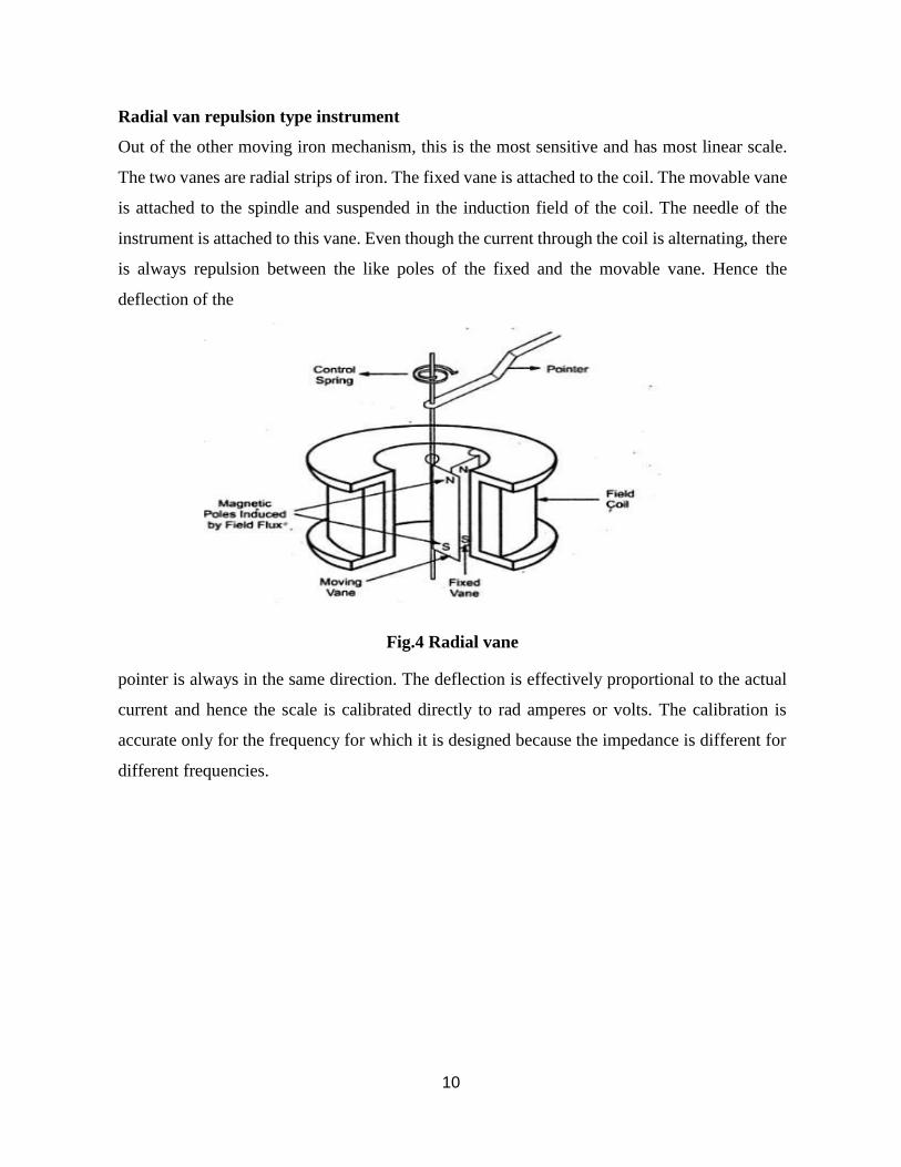
Radial van repulsion type instrument

Out of the other moving iron mechanism, this is the most sensitive and has most linear scale.

The two vanes are radial strips of iron. The fixed vane is attached to the coil. The movable vane

is attached to the spindle and suspended in the induction field of the coil. The needle of the

instrument is attached to this vane. Even though the current through the coil is alternating, there

is always repulsion between the like poles of the fixed and the movable vane. Hence the

deflection of the

Fig.4 Radial vane

pointer is always in the same direction. The deflection is effectively proportional to the actual

current and hence the scale is calibrated directly to rad amperes or volts. The calibration is

accurate only for the frequency for which it is designed because the impedance is different for

different frequencies.

11

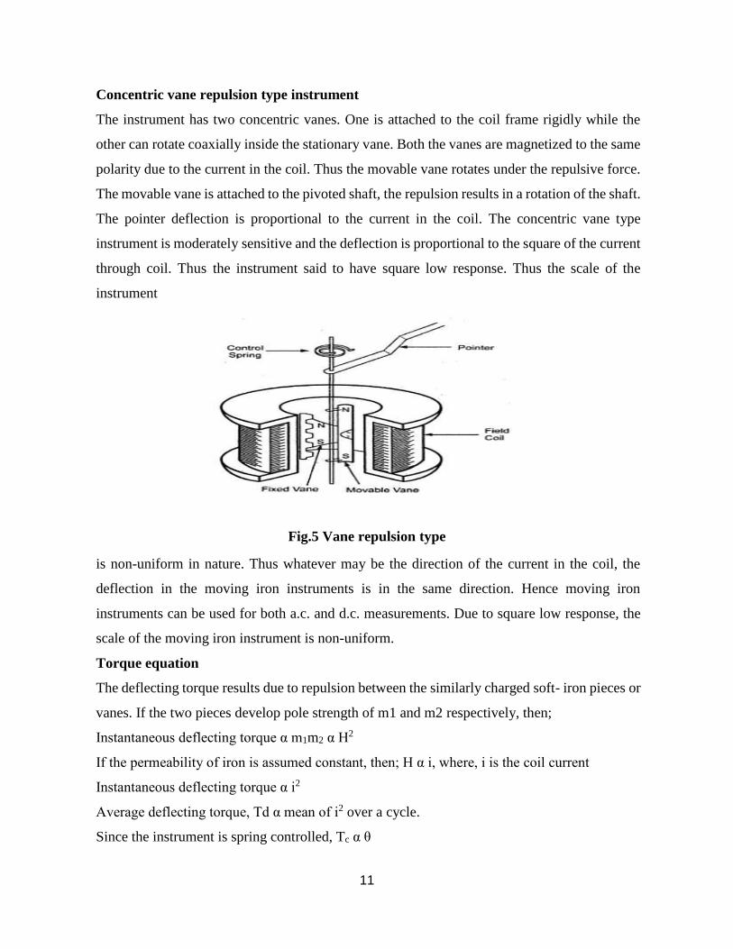
Concentric vane repulsion type instrument

The instrument has two concentric vanes. One is attached to the coil frame rigidly while the

other can rotate coaxially inside the stationary vane. Both the vanes are magnetized to the same

polarity due to the current in the coil. Thus the movable vane rotates under the repulsive force.

The movable vane is attached to the pivoted shaft, the repulsion results in a rotation of the shaft.

The pointer deflection is proportional to the current in the coil. The concentric vane type

instrument is moderately sensitive and the deflection is proportional to the square of the current

through coil. Thus the instrument said to have square low response. Thus the scale of the

instrument

Fig.5 Vane repulsion type

is non-uniform in nature. Thus whatever may be the direction of the current in the coil, the

deflection in the moving iron instruments is in the same direction. Hence moving iron

instruments can be used for both a.c. and d.c. measurements. Due to square low response, the

scale of the moving iron instrument is non-uniform.

Torque equation

The deflecting torque results due to repulsion between the similarly charged soft- iron pieces or

vanes. If the two pieces develop pole strength of m1 and m2 respectively, then;

Instantaneous deflecting torque α m1m2 α H2

If the permeability of iron is assumed constant, then; H α i, where, i is the coil current

Instantaneous deflecting torque α i2

Average deflecting torque, Td α mean of i2 over a cycle.

Since the instrument is spring controlled, Tc α θ

12

In the steady position of deflection, Td = Tc

θ α mean of i2 over a cycle.

α I2

Thus, the deflection is proportional to the square of the coil current. The scale of the instrument

is non- uniform; being crowded in the beginning and spread out near the finish end of the scale.

However, the non- linearity of the scale can be corrected to some extent by the accurate shaping

and positioning of the iron vanes in relation to the operating coil.

Advantages

1) The instruments can be used for both a.c. and d.c. measurements.

2) As the torque to weight ratio is high, errors due to the friction are very less.

3) A single type of moving element can cover the wide range hence these instruments are

cheaper than other types of if instruments.

4) There are no current carrying parts in the moving system hence these meters are extremely

rugged and reliable.

5) These are capable of giving good accuracy. Modern moving iron instruments have a

d.c. error of 2% or less.

6) These can withstand large loads and are not damaged even under sever overload conditions.

7) The range of instruments can be extended.

Disadvantages

1) The scale of moving iron instruments is not uniform and is cramped at the lower end. Hence

accurate readings are not possible at this end.

2) There are serious errors due to hysteresis, frequency changes and stray magnetic fields.

3) The increase in temperature increases the resistance of coil, decreases stiffness of the

springs, decreases the permeability and hence affect the reading severely.

4) Due to the non linearity of B-H curve, the deflecting torque is not exactly proportional to the

square of the current.

5) There is a difference between a.c. and d.c. calibration on account of the effect of inductance

of the meter. Hence these meters must always be calibrated at the frequency at which they are

to be used. The usual commercial moving iron instrument may be used within its specified

accuracy from 25 to 125 HZ frequency range.

6) Power consumption is on higher side.

13

Errors in moving iron instrument

1) Hysteresis error: Due to hysteresis effect, the flux density for the same current while

ascending and descending values is different. While descending, the flux density is higher and

while ascending it is lesser. So meter reads higher for descending values of current or voltage.

So remedy for this is to use smaller iron parts which can demagnetise quickly or to work with

lower flux densities.

2) Temperature error: The temperature error arises due to the effect of temperature on the

temperature coefficient of the spring. This error is of the order of 0.02 % change in temperature.

Errors can cause due to self-heating of the coil and due to which change in resistance of the

coil. So coil and series resistance must have low temperature coefficient. Hence mangnin is

generally used for the series resistance.

3) Stray magnetic Field Error: The operating magnetic field in case of moving iron

instruments is very low. Hence effect of external i.e. stray magnetic field can cause

error. This effect depends on the direction of the stray magnetic field with respect to the

operating field of the instrument.

4) Frequency Error : These are related to a.c. operation of the instrument. The change in

frequency affects the reactance of the working coil and also affects the magnitude of the eddy

currents. This cause error in the instrument.

5) Eddy Current Error : When instrument is used for a.c. measurements the eddy currents

are produced in the iron parts of the instrument. The eddy current affects the instrument current

causing the change in the deflection torque. This produce the error in the meter reading. As

eddy current are frequency dependent, frequency changes cause eddy current error.

14

4. DYNAMAOMETER

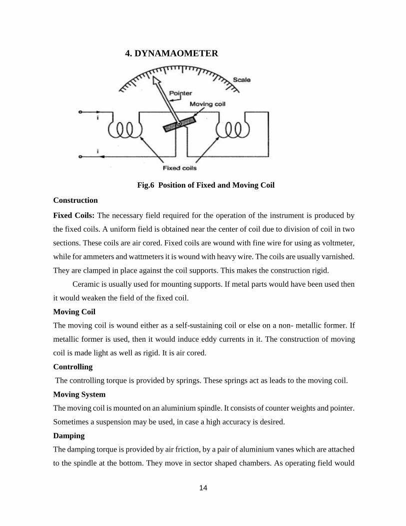
Fig.6 Position of Fixed and Moving Coil

Construction

Fixed Coils: The necessary field required for the operation of the instrument is produced by

the fixed coils. A uniform field is obtained near the center of coil due to division of coil in two

sections. These coils are air cored. Fixed coils are wound with fine wire for using as voltmeter,

while for ammeters and wattmeters it is wound with heavy wire. The coils are usually varnished.

They are clamped in place against the coil supports. This makes the construction rigid.

Ceramic is usually used for mounting supports. If metal parts would have been used then

it would weaken the field of the fixed coil.

Moving Coil

The moving coil is wound either as a self-sustaining coil or else on a non- metallic former. If

metallic former is used, then it would induce eddy currents in it. The construction of moving

coil is made light as well as rigid. It is air cored.

Controlling

The controlling torque is provided by springs. These springs act as leads to the moving coil.

Moving System

The moving coil is mounted on an aluminium spindle. It consists of counter weights and pointer.

Sometimes a suspension may be used, in case a high accuracy is desired.

Damping

The damping torque is provided by air friction, by a pair of aluminium vanes which are attached

to the spindle at the bottom. They move in sector shaped chambers. As operating field would

15

be distorted by eddy current damping, it is not employed.

Shielding

The field produced by these instruments is very weak. Even earth's magnetic field considerably

affects the reading. So shielding is done to protect it from stray magnetic fields. It is done by

enclosing in a casing high permeability alloy.

Cases and Scales

Laboratory standard instruments are usually contained in polished wooden or metal cases

which are rigid. The case is supported by adjustable levelling screws. A spirit level may be

provided to ensure proper levelling. For using electrodynamometer instrument as ammeter,

fixed and moving coils are connected in series and carry the same current. A suitable shunt is

connected to these coils to limit current through them upto desired limit. The

electrodynamometer instruments can be used as a voltmeter by connecting the fixed and moving

coils in series with a high non-inductive resistance. It is most accurate type of voltmeter.

For using electrodynamometer instrument as a wattmeter to measure the power, the fixed

coils acts as a current coil and must be connected in series with the load. The moving coils acts

as a voltage coil or pressure oil and must be connected across the supply terminals. The

wattmeter indicates the supply power.

Working

When current passes through the fixed and moving coils, both coils produce the magnetic

fields. The field produced by fixed coil is proportional to the load current while the field

produced by the moving coil is proportional to the voltage. As the deflecting torque is produced

due to the interaction of these two fields, the deflection is proportional to the power supplied to

the load.

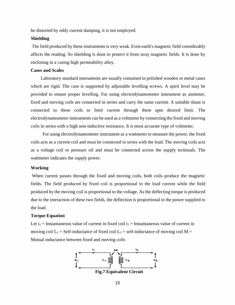
Torque Equation

Let i1 = Instantaneous value of current in fixed coil i2 = Instantaneous value of current in

moving coil L1 = Self-inductance of fixed coil L2 = self-inductance of moving coil M =

Mutual inductance between fixed and moving coils

Fig.7 Equivalent Circuit

16

The electrodynamometer instrument can be represented by an equivalent circuit,

From the principle of conversation of energy,

Energy input=Energy stored + Mechanical energy

Mechanical energy=energy input-energy stored

Subtraction (2) from equation (1),

The self inductance L1 and L2 are constant and hence dL1 and dL2 are zero. Mechanical energy

= i1i2dM

If Ti is the instantaneous deflecting torque and dθ is the change in the deflection then

Mechanical energy = Mechanical work done

=Ti dθ i1 i2 d M = Ti dθ

17

Advantage of Electrodynamometer instrument

1) As the coils are air cored, these instruments are free from hysteresis and eddy

current losses.

2) They have a precision grade security.

3) These instruments can be used on both a.c. and d.c. They are also used as a

transfer instruments.

4) Electrodynamometer voltmeter are very useful where accurate r.m.s values of

voltage, irrespective of waveforms, are required.

5) Free from hysteresis errors.

6) Low power Consumption.

7) Light in weight.

Disadvantage of electrodynamometer instrument

1) These instruments have a low sensitivity due to a low torque to weight ratio. Also it

introduces increased frictional losses. To get accurate results, these errors must be

minimized.

2) They are more expensive than other type of instruments.

3) These instruments are sensitive to overload and mechanical impacts. Therefore can must

be taken while handling them.

4) They have a nonuniform scale.

5) The operation current of these instruments is large due to the fact that they have weak

magnetic field

Error in electrodynamometer instrument

The various errors in electrodynamometer instruments are,

1. Torque to weight ratio : To have reasonable deflecting torque, mmf of the moving coil

must be large enough. Thus m.m.f. = NI hence current through moving coil should be high or

number of turns should be large. The current cannot be made very high because it may cause

excessive heating of springs. Large number of turns hence is the only option but it increases

weight of the coil. This makes the system heavy reducing torque to weight ratio. This can cause

frictional errors in the reading

2. Frequency errors : The changes in the frequency causes to change self inductances of

moving coil and fixed coil. This causes the error in the reading. The frequency error can be

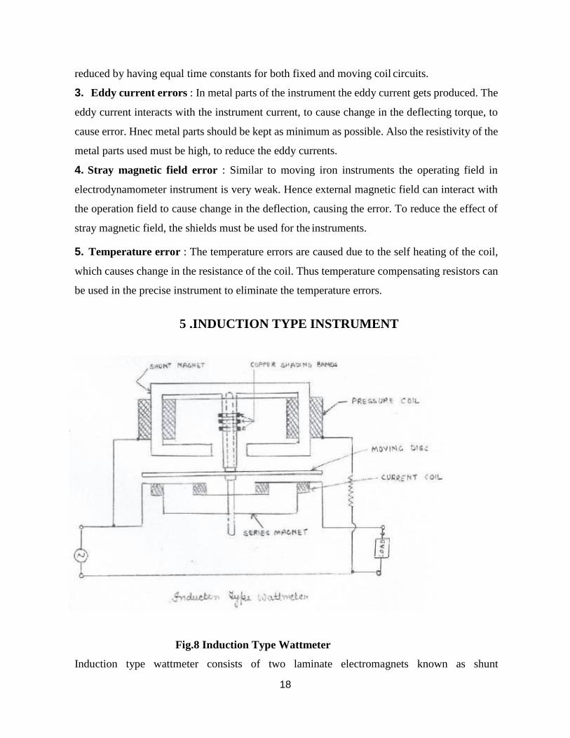
18

reduced by having equal time constants for both fixed and moving coil circuits.

3. Eddy current errors : In metal parts of the instrument the eddy current gets produced. The

eddy current interacts with the instrument current, to cause change in the deflecting torque, to

cause error. Hnec metal parts should be kept as minimum as possible. Also the resistivity of the

metal parts used must be high, to reduce the eddy currents.

4. Stray magnetic field error : Similar to moving iron instruments the operating field in

electrodynamometer instrument is very weak. Hence external magnetic field can interact with

the operation field to cause change in the deflection, causing the error. To reduce the effect of

stray magnetic field, the shields must be used for the instruments.

5. Temperature error : The temperature errors are caused due to the self heating of the coil,

which causes change in the resistance of the coil. Thus temperature compensating resistors can

be used in the precise instrument to eliminate the temperature errors.

5 .INDUCTION TYPE INSTRUMENT

Fig.8 Induction Type Wattmeter

Induction type wattmeter consists of two laminate electromagnets known as shunt

19

electromagnet and series electromagnet respectively. Shunt magnet is excited by the current

proportional to the voltage across load flowing through the pressure coil and series magnet is

excited by the current, proportional to the voltage across the load flowing through the pressure

coil and series magnet is excited by the load current flowing through the current coil. A thin

disc made of Cu or Al, pivoted at its centre, is placed between the shunt and series magnets so

that it cuts the flux from both of the magnets. The deflection torque is produced by interaction

of eddy current induced in the disc and the inducing flux in order to cause the resultant flux

in shunt magnet to lag in phase by exactly 90° behind the applied voltage, one or more copper

rings, known as copper shading bond are provided on one limb at the shunt magnet. Correct

disappointed between shunt and series magnet fluxes may be attained by adjusting the position

of copper shading bonds. The pressure coil circuit of introduction type instrument is made

6. THERMAL TYPE INSTRUMENT

The hot wire instruments are based on the principle that length of wire increases due to heating

effect when a current passed through it. It is a square law device with a non- linear relationship

because increase in length of a wire is directly proportional to the square of current passing

through wire. Note that the increase in the length of a wire is very small percentage of the total

length of wire. Hence various mechanical linkages have been devised to expand this effect and

convert it into motion of a point of a circular

scale.

Fig.9 Thermal Type Instrument

A hot working wire denoted by W in the Figure is made up of platinum-irridum alloy. The main

20

advantages of using platinum-irridum alloy is that it can withstand high temperatures without

deterioration of wire material caused by oxidation. The working wire W is very fine and its

diameter is of the order of 0.1 mm. The wire W is stretched between two point A and B where

point B is fixed point and point A is tension adjustment point at which tension adjustment

mechanism is placed. One more wire W1, made up of phosphor-bronze is connected to main

hot wire W at point C while other end of wire W1 is connected to fixed point D. A fine thread

of silk material represented by G is connected between spring S and point F. The thread G is

wound around a pulley denoted by E. Both points F and spring S are fixed points. A point P

used for indication and thin aluminium disc L are mounted on the spindle. The pulley system E

is also mounted on the spindle.

When a current to be measured is passed through the wire, it gets expanded as a result of heating

effect by current flowing through it. Because of heating effect, a sag is produced in the wire W.

Now the sag in main working wire W causes sag in other wire W1. This sag is transferred to

the spring S through a fine silk thread G. Thus the sag produced gets magnified and the spring

activates pulley to rotate and pointer gets deflected indicating value of the current under

measurement on a graduated scale.

The expansion of the wire is proportional to the heating effect of the current. As heat produced

is in the form of power dissipated give P = I2R , the expansion of the wire in hot wire instrument

is proportional to the square of r.m.s. value of the current. A thin aluminium disc L rotates

between poles of the permanent magnet M and it provides eddy current damping to the

instrument. The base of the main instrument is made up of a material which is having coefficient

of expansion same as that of hot wire. As base and hot wire, both have same coefficient of

expansion, the errors due to uneven expansion between base of instrument and hot wire are

minimized.

In early hot wire instruments, the hot wire used was made up of platinum-silver alloy. But the

main drawback of early instruments was the low value of the full-scale operating temperature

(about 135-150 oC). Because of very low operating temperature, even small variations in room

temperature affects the position of the pointer. Today's hot wire instruments use wire made up

of platinum-irridum alloy with which operating temperature range can be extended upto 300 to

500 oC. As the temperature range is increased, the effects due to room temperature variations

21

are minimized. The hot wire is made very thin so that it can attain steady temperature quickly

when current flows through wire. The size of wire is decided such that it can bare normal

mechanical stresses developed in the instruments.

The hot wire instrument can be used as ammeter over a range 0 to 1 A without a shunt, while 0

to 5 A with a shunt. It can be used as a voltmeter to measure voltage upto 400 V by using high

value non-inductive resistance in series with instruments.

Advantages of hot wire type instrument

(i) no stray magnetic field effect

(ii) same calibration for dc as well as for ac

(iii) fair accuracy

(iv) simple construction

(v) low cost

(vi) negligible temperature error if suitably adjusted and

(vii) suitability for measurement of currents at very high frequencies

Disadvantages of hot wire type instrument

(i) delicate construction

(ii) relatively higher power consumption

(iii) uneven scale

(iv) incapability of taking over-load

(v) sluggish in action

(vi) need of frequent adjustment of zero position due to temperature variations and

(viii) different deflections for ascending and descending values.

7. RECTIFIER TYPE INSTRUMENT

Rectifier type instrument measures the alternating voltage and current with the help of

rectifying elements and permanent magnet moving coil type of instrument However the primary

function of rectifier type of instruments work as voltmeter

We have used here a bridge rectifier circuit as shown. Again we divide our operation into two

parts. In the first we analyze the output by applying the dc voltage and in another we will apply

ac voltage to the circuit. A series multiplier resistance is connected in series with the voltage

source which has the same function as described above.

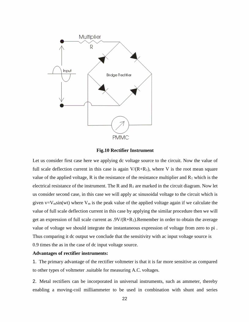
22

Fig.10 Rectifier Instrument

Let us consider first case here we applying dc voltage source to the circuit. Now the value of

full scale deflection current in this case is again V/(R+R1), where V is the root mean square

value of the applied voltage, R is the resistance of the resistance multiplier and R1 which is the

electrical resistance of the instrument. The R and R1 are marked in the circuit diagram. Now let

us consider second case, in this case we will apply ac sinusoidal voltage to the circuit which is

given v=Vmsin(wt) where Vm is the peak value of the applied voltage again if we calculate the

value of full scale deflection current in this case by applying the similar procedure then we will

get an expression of full scale current as .9V/(R+R1).Remember in order to obtain the average

value of voltage we should integrate the instantaneous expression of voltage from zero to pi .

Thus comparing it dc output we conclude that the sensitivity with ac input voltage source is

0.9 times the as in the case of dc input voltage source.

Advantages of rectifier instruments:

1. The primary advantage of the rectifier voltmeter is that it is far more sensitive as compared

to other types of voltmeter .suitable for measuring A.C. voltages.

2. Metal rectifiers can be incorporated in universal instruments, such as ammeter, thereby

enabling a moving-coil milliammeter to be used in combination with shunt and series

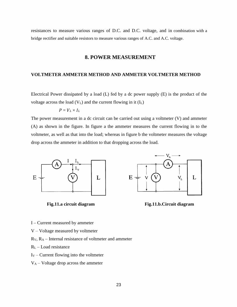
23

resistances to measure various ranges of D.C. and D.C. voltage, and in combination with a

bridge rectifier and suitable resistors to measure various ranges of A.C. and A.C. voltage.

8. POWER MEASUREMENT

VOLTMETER AMMETER METHOD AND AMMETER VOLTMETER METHOD

Electrical Power dissipated by a load (L) fed by a dc power supply (E) is the product of the

voltage across the load (VL) and the current flowing in it (IL)

𝑃 = 𝑉𝐿 × 𝐼𝐿

The power measurement in a dc circuit can be carried out using a voltmeter (V) and ammeter

(A) as shown in the figure. In figure a the ammeter measures the current flowing in to the

voltmeter, as well as that into the load; whereas in figure b the voltmeter measures the voltage

drop across the ammeter in addition to that dropping across the load.

Fig.11.a circuit diagram Fig.11.b.Circuit diagram

I – Current measured by ammeter

V – Voltage measured by voltmeter

RV, RA – Internal resistance of voltmeter and ammeter

RL – Load resistance

IV – Current flowing into the voltmeter

VA – Voltage drop across the ammeter

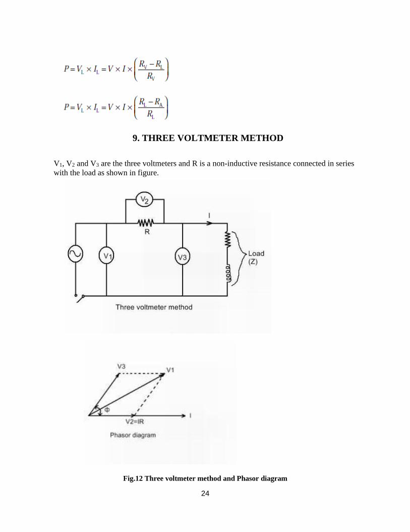
24

9. THREE VOLTMETER METHOD

V1, V2 and V3 are the three voltmeters and R is a non-inductive resistance connected in series

with the load as shown in figure.

Fig.12 Three voltmeter method and Phasor diagram

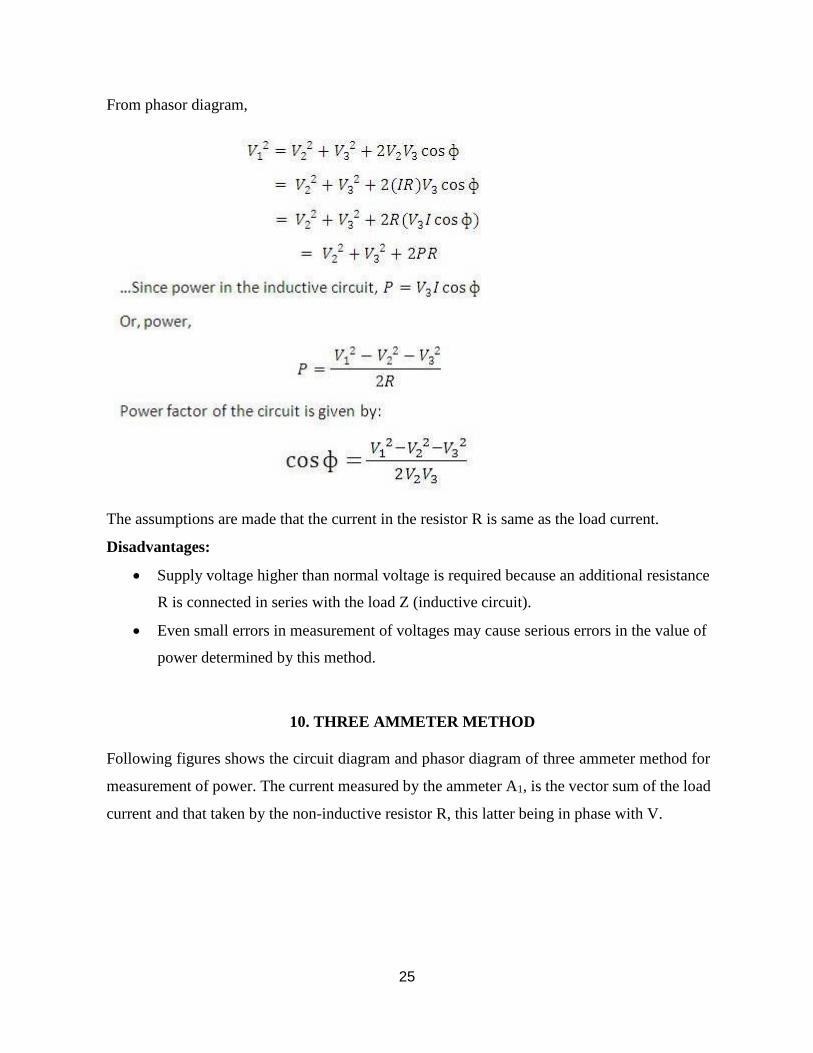
25

From phasor diagram,

The assumptions are made that the current in the resistor R is same as the load current.

Disadvantages:

Supply voltage higher than normal voltage is required because an additional resistance

R is connected in series with the load Z (inductive circuit).

Even small errors in measurement of voltages may cause serious errors in the value of

power determined by this method.

10. THREE AMMETER METHOD

Following figures shows the circuit diagram and phasor diagram of three ammeter method for

measurement of power. The current measured by the ammeter A1, is the vector sum of the load

current and that taken by the non-inductive resistor R, this latter being in phase with V.

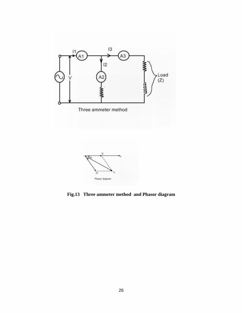
26

Fig.13 Three ammeter method and Phasor diagram

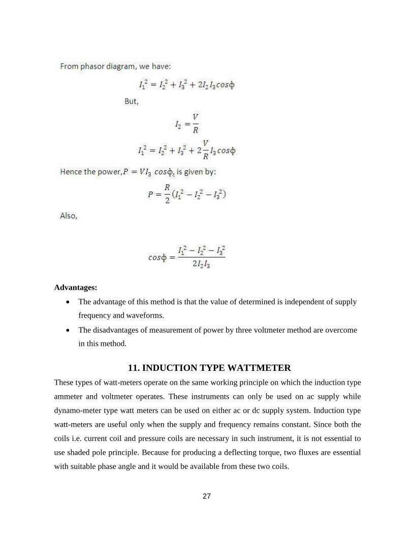
27

Advantages:

The advantage of this method is that the value of determined is independent of supply

frequency and waveforms.

The disadvantages of measurement of power by three voltmeter method are overcome

in this method.

11. INDUCTION TYPE WATTMETER

These types of watt-meters operate on the same working principle on which the induction type

ammeter and voltmeter operates. These instruments can only be used on ac supply while

dynamo-meter type watt meters can be used on either ac or dc supply system. Induction type

watt-meters are useful only when the supply and frequency remains constant. Since both the

coils i.e. current coil and pressure coils are necessary in such instrument, it is not essential to

use shaded pole principle. Because for producing a deflecting torque, two fluxes are essential

with suitable phase angle and it would be available from these two coils.

28

A watt-meter has two laminated electromagnet, one of which is excited by load current or

definite fraction of it, and is connected in series with the circuit, known as series magnet and

the other is excited by the current proportional to the applied voltage or fraction of it and is

always connected across the supply, known as shunt magnet. An aluminum disc is so mounted

so that it cuts the fluxes produced by both the magnets. As a result of which, two e.m.f are

produced which induces two eddy currents in the disc. C - Magnet is used to provide necessary

damping torque to the pointer, to damp out the oscillations. Deflecting torque is produced due

to interaction of these eddy currents and the inducing flux. Copper shading bands are provided

either on central limb or on the outer limb of the shunt magnet, and can be so adjusted as to

make the resultant flux in the shunt magnet lag behind the applied voltage by 90. Both the watt-

meters are provided with spiral springs A and B, for producing controlling torque to counter

balance the deflecting torque. In Fig.a the spiral spring and damping magnet is omitted for

simplicity. The scale of such type instruments is quite uniform and extends over an angle of

300. Currents up to 100 A can be handled by these watt-meters directly where as beyond this

current transformers are used. Two types of induction type watt meters are available. Line

diagrams of both of the types are detailed in Figures a and b.

Fig.14 Induction type Wattmeter

In the form of the instrument shown in Fig. a, two pressure coils are connected in series in such

a way that both of them send flux through the central limb. The series magnet

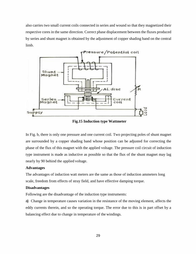
29

also carries two small current coils connected in series and wound so that they magnetized their

respective cores in the same direction. Correct phase displacement between the fluxes produced

by series and shunt magnet is obtained by the adjustment of copper shading band on the central

limb.

Fig.15 Induction type Wattmeter

In Fig. b, there is only one pressure and one current coil. Two projecting poles of shunt magnet

are surrounded by a copper shading band whose position can be adjusted for correcting the

phase of the flux of this magnet with the applied voltage. The pressure coil circuit of induction

type instrument is made as inductive as possible so that the flux of the shunt magnet may lag

nearly by 90 behind the applied voltage.

Advantages

The advantages of induction watt meters are the same as those of induction ammeters long

scale, freedom from effects of stray field, and have effective damping torque.

Disadvantages

Following are the disadvantage of the induction type instruments:

a) Change in temperature causes variation in the resistance of the moving element, affects the

eddy currents therein, and so the operating torque. The error due to this is in part offset by a

balancing effect due to change in temperature of the windings.

30

b) Change in frequency from that of the calibration value causes variations in both the reactance

of the voltage coil circuit, which is highly inductive, and also in the amount of compensation

from the phase compensating circuit. Within the limits of frequency variation met within

practice on the mains, this last error in not important.

12. ELECTRODYNAMOMETER WATTMETER

Dynamometer type wattmeter works on very simple principle and this principle can be stated

as "when any current carrying conductor is placed inside a magnetic field, it experiences a

mechanical force and due this mechanical force deflection of conductor takes place".

Construction and Working Principle

. It consists of following parts

Fig.16 Electrodynamometer

There are two types of coils present in the electrodynamometer. They are :

(a) Moving coil : Moving coil moves the pointer with the help of spring control instrument. A

limited amount of current flows through the moving coil so as to avoid heating. So in order

to limit the current we have connect the high value resistor in series with the moving coil. The moving

is air cored and is mounted on a pivoted spindle and can moves freely. In electrodynamometer type

wattmeter, moving coil works as pressure coil. Hence moving coil is connected across the voltage and

thus the current flowing through this coil is always proportional to the voltage.

(b) Fixed coil: The fixed coil is divided into two equal parts and these are connected in series

with the load, therefore the load current will flow through these coils. Now the reason is very

obvious of using two fixed coils instead of one, so that it can be constructed to carry

considerable amount of electric current. These coils are called the current coils of

electrodynamometer type wattmeter. Earlier these fixed coils are designed to carry the current

31

of about 100 amperes but now the modern wattmeter are designed to carry current of about 20

amperes in order to save power.

(c) Control system: Out of two controlling systems i.e.

(1) Gravity control

(2) Spring control, only spring controlled systems are used in these types of wattmeter. Gravity

controlled system cannot be employed because they will appreciable amount of errors.

(d) Damping system: Air friction damping is used, as eddy current damping will distort the

weak operating magnetic field and thus it may leads to error.

(e) Scale: There is uniform scale is used in these types of instrument as moving coil moves

linearly over a range of 40 degrees to 50 degrees on either sides.

Now let us derive the expressions for the controlling torque and deflecting torques. In order to

derive these expressions let us consider the circuit diagram given

We know that instantaneous torque in electrodynamic type instruments is directly proportional

to product of instantaneous values of currents flowing through both the coils and the rate of

change of flux linked with the circuit.

Let I1 and I2 be the instantaneous values of currents in pressure and current coils respectively.

So the expression for the torque can be written as:

𝑑𝑀 𝑇 = 1 × 𝐼2 ×

𝑑𝑥

where x is the angle.

Now let the applied value of voltage across the pressure coil be

= 2𝑉 sin 𝜔𝑡

Assuming the electrical resistance of the pressure coil be very high hence we can neglect

reactance with respect to its resistance. In this the impedance is equal to its electrical resistance

therefore it is purely resistive.The expression for instantaneous current can be written as I2 = v

/ Rp where Rp is the resistance of pressure coil.

𝑉 sin 𝜔𝑡

𝐼2 = 2 × 𝑅𝑝

If there is phase difference between voltage and electric current, then expression for

instantaneous current through current coil can be written as

32

𝐼1 = 𝐼 𝑡 = 2𝐼 sin(𝜔𝑡 − ∅)

As current through the pressure coil in very very small compare to current through current coil

hence current through the current coil can be considered as equal to total load current.

Hence the instantaneous value of torque can be written as

2 × 𝑉 sin 𝜔𝑡

𝑅𝑝

× 2𝐼 sin 𝜔𝑡 − ∅ 𝑑𝑀

𝑑𝑥

33

Average value of deflecting torque can be obtained by integrating the instantaneous torque

from limit 0 to T, where T is the time period of the cycle.Controlling torque is given by Tc =

Kx where K is spring constant and x is final steady state value of deflection.

Advantages of Electrodynamometer Type Wattmeter

Following are the advantages of electrodynamometer type wattmeters and they are written as

follows:

(a) Scale is uniform upto certain limit.

(b) They can be used for both to measure ac as well dc quantities as scale is calibrated for

both.

Errors in Electrodynamometer Type Wattmeter

Following are the errors in the electrodynamometer type wattmeters:

(a) Errors in the pressure coil inductance

(b) Errors may be due to pressure coil capacitance

(c) Errors may be due to mutual inductance effects

(d) Errors may be due connections (i.e. pressure coil is connected after current coil)

(e) Error due to Eddy currents

(f) Errors caused by vibration of moving system

(g) Temperature error

(h) Errors due to stray magnetic field

MEASUREMENT OF THREE PHASE POWER BY TWO WATTMETERS METHOD

In this method we have two types of connections

(a)Star connection of loads

(b)Delta connection of loads

When the star connected load, the diagram is shown in below- (c) Errors may be due to

mutual inductance effects

(d) Errors may be due connections (i.e. pressure coil is connected after current coil)

(e) Error due to Eddy currents

(f) Errors caused by vibration of moving system

(g) Temperature error

(h) Errors due to stray magnetic field

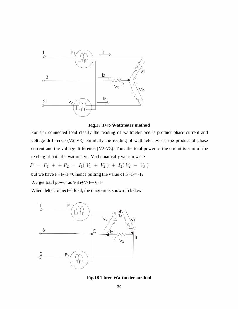
34

Fig.17 Two Wattmeter method

For star connected load clearly the reading of wattmeter one is product phase current and

voltage difference (V2-V3). Similarly the reading of wattmeter two is the product of phase

current and the voltage difference (V2-V3). Thus the total power of the circuit is sum of the

reading of both the wattmeters. Mathematically we can write

but we have I1+I2+I3=0,hence putting the value of I1+I2= -I3

We get total power as V1I1+V2I2+V3I3

When delta connected load, the diagram is shown in below

Fig.18 Three Wattmeter method

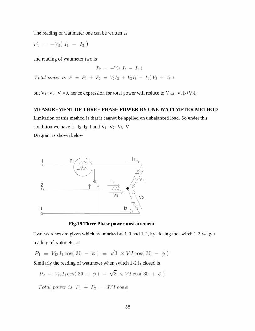
35

The reading of wattmeter one can be written as

and reading of wattmeter two is

but V1+V2+V3=0, hence expression for total power will reduce to V1I1+V2I2+V3I3

MEASUREMENT OF THREE PHASE POWER BY ONE WATTMETER METHOD

Limitation of this method is that it cannot be applied on unbalanced load. So under this

condition we have I1=I2=I3=I and V1=V2=V3=V

Diagram is shown below

Fig.19 Three Phase power measurement

Two switches are given which are marked as 1-3 and 1-2, by closing the switch 1-3 we get

reading of wattmeter as

Similarly the reading of wattmeter when switch 1-2 is closed is

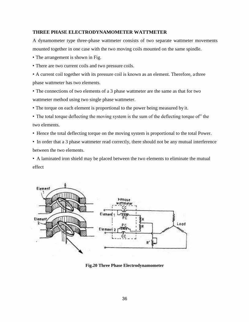
36

THREE PHASE ELECTRODYNAMOMETER WATTMETER

A dynamometer type three-phase wattmeter consists of two separate wattmeter movements

mounted together in one case with the two moving coils mounted on the same spindle.

• The arrangement is shown in Fig.

• There are two current coils and two pressure coils.

• A current coil together with its pressure coil is known as an element. Therefore, a three

phase wattmeter has two elements.

• The connections of two elements of a 3 phase wattmeter are the same as that for two

wattmeter method using two single phase wattmeter.

• The torque on each element is proportional to the power being measured by it.

• The total torque deflecting the moving system is the sum of the deflecting torque of‟ the

two elements.

• Hence the total deflecting torque on the moving system is proportional to the total Power.

• In order that a 3 phase wattmeter read correctly, there should not be any mutual interference

between the two elements.

• A laminated iron shield may be placed between the two elements to eliminate the mutual

effect

Fig.20 Three Phase Electrodynamometer

37

LOW POWER FACTOR ELECTRO-DYNAMOMETER TYPE WATTMETERS

Small deflecting torque on the moving system even when the current and pressure coils

are fully excited and

Introduction of large error due to inductance of pressure coil at low power factor.

The special features incorporated in an electro-dynamometer type wattmeter to make it

suitable for measurement of power in low power factor circuits are given below.

1. Pressure coil Circuit. The pressure coil circuit is made of low resistance in order to make

the pressure coil current large resulting in increased operating torque. The pressure coil

current in a low pf wattmeter may be as much as 10 times the value used for ordinary

wattmeters.

2. Compensation For Pressure Coil current

3. Compensation For Inductance of Pressure Coil. The error caused by pressure coil

inductance is (sinΘ)/cos Ø + sinΘ times the actual reading of wattmeter. Now with low

pf, the value of Ø is large and, therefore, the error is large. The error caused by inductance

of pressure coil is compensated by connecting a capacitor across a part of series

resistance in the pressure coil circuit, as shown in fig

Fig.21 low Power factor Electro dynamometer

38

Reference books

1. Sawhney A.K., “A Course in Electrical, Electronic measurement &

Instrumentation”, Dhanpat Rai & sons, 18th Edition, Reprint 2010.

2. Doebelin E.O., “Measurement System Applications and Design”, McGraw Hill,

5th Edition, 2004.

3. Jain R.K., “Mechanical and Industrial Measurements”, Khanna Publishers, 11th

edition, Reprint 2005.

4. Jones’ Instrument Technology, Instrumentation Systems, Edited by B.E.Noltingk,

Vol 4, 4th edition, ELBS, 1987.

5. Murthy D.V.S., “Transducers and Instrumentation”, Printice Hall of India, 13th

printing, 2006.

6. Gnanavadivel,“Measurements and Instrumentation”,Anuradha Publication, Second

Revised Edition 2011.

1

SCHOOL OF ELECTRICAL AND ELECTRONICS

DEPARTMENT OF ELECTRICAL AND ELECTRONICS

UNIT – III

MEASUREMENT AND INSTRUMENTATION – SIC 1203

2

UNIT 3 MEASUREMENT OF RESISTANCE, INDUCTANCE AND CAPACITANCE

Low Resistance: Kelvin's double bridge - Medium Resistance: Voltmeter Ammeter

method – Substitution method - Wheatstone bridge method. High Resistance: Megger -

Direct deflection method - Megohm bridge method, Loss of Charge method - Earth

resistance measurement. Introduction to A.C bridges Sources and Detectors in A.C.

bridges. Measurement of Self Inductance: Maxwell's bridge - Hay's bridge, and

Anderson's bridge. Measurement of Mutual Inductance: Heaviside M.I bridge -

Measurement of Capacitance: Schering's bridge – De Sauty's bridge, Measurement of

frequency using Wien's bridge.

CLASSIFICATION OF RESISTANCES

For the purposes of measurements, the resistances are classified into three major groups

based on their numerical range of values as under:

• Low resistance (0 to 1 ohm)

• Medium resistance (1 to 100 kilo-ohm) and

• High resistance (>100 kilo-ohm)

Accordingly, the resistances can be measured by various ways, depending on their range of

values, as under:

1. Low resistance (0 to 1 ohm): AV Method, Kelvin Double Bridge, potentiometer, doctor

ohmmeter, etc.

2. Medium resistance (1 to 100 kilo-ohm): AV method, wheat stone’s bridge, substitution

method, etc.

3. High resistance (>100 kilo-ohm): AV method, Fall of potential method, Megger, loss of

charge method, substitution method, bridge method, etc.

1. LOW RESISTANCE

1.1 KELVIN DOUBLE BRIDGE

The Kelvin double bridge is one of the best devices available for the precise measurement of

low resistances. It is the modification of wheatstone bridge by which the errors due to contact

resistance and lead resistances are eliminated. This bridge is named double bridge because it

contains a second set of ratio arms. An interesting variation of the Wheatstone bridge is the

Kelvin Double bridge, used for measuring very low resistances (typically less than 1/10 of an

ohm)

THEORY

Consider the bridge circuit shown in figure below. Here ‘r’ represents the resistance of the lead

that connects the unknown resistance ‘R’ to standard resistance ‘S’. Two galvanometer

3

connections indicated by dotted lines are possible. The connection may be either to point 'm'

or to point 'n'. When the galvanometer is connected to point ‘m’ the resistance ‘ r’ of the

connecting leads is added to the standard resistance ‘S’ resulting in indication of too low an

indication for unknown resistance ‘R’. When the connection made to point the resistance ‘r’ is

added to the unknown resistance resulting in indication of too high a value for ‘R’.

Suppose that instead of using point ‘m’ which gives a low result or ‘n’ which makes the result

High, we make the galvanometer connection to any intermediate point‘d’ as shown by full line.

If at point‘d’ the resistance ‘r’ is divided into two parts r1, r2 such that r1/r2 = P/Q

Fig.1 Circuit Diagram

The kelvin’s double bridge incorporates the idea of a second set of ratio arms - hence the name

double bridge- and the use of four terminal resistors for the low resistance arms.

1st R1/R2 2nd a/b

4

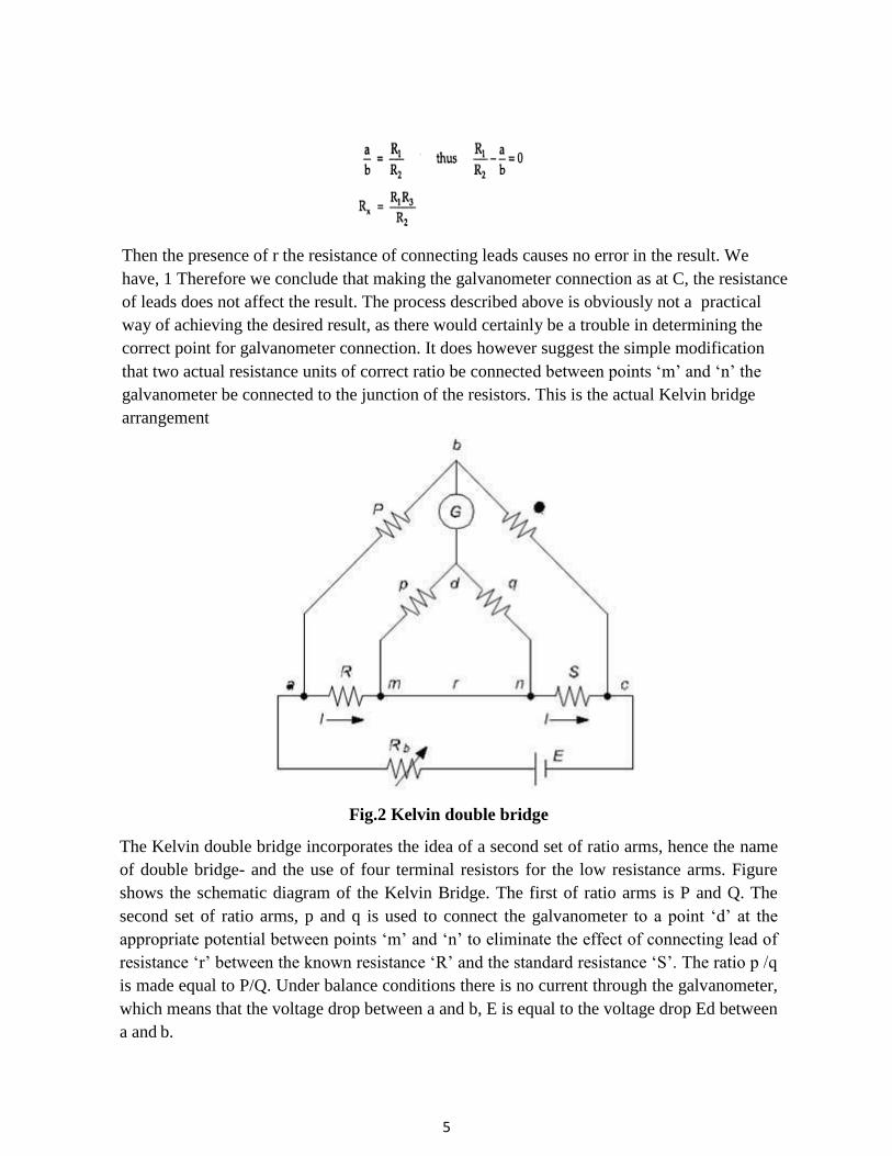
5

Then the presence of r the resistance of connecting leads causes no error in the result. We

have, 1 Therefore we conclude that making the galvanometer connection as at C, the resistance

of leads does not affect the result. The process described above is obviously not a practical

way of achieving the desired result, as there would certainly be a trouble in determining the

correct point for galvanometer connection. It does however suggest the simple modification

that two actual resistance units of correct ratio be connected between points ‘m’ and ‘n’ the

galvanometer be connected to the junction of the resistors. This is the actual Kelvin bridge

arrangement

Fig.2 Kelvin double bridge

The Kelvin double bridge incorporates the idea of a second set of ratio arms, hence the name

of double bridge- and the use of four terminal resistors for the low resistance arms. Figure

shows the schematic diagram of the Kelvin Bridge. The first of ratio arms is P and Q. The

second set of ratio arms, p and q is used to connect the galvanometer to a point ‘d’ at the

appropriate potential between points ‘m’ and ‘n’ to eliminate the effect of connecting lead of

resistance ‘r’ between the known resistance ‘R’ and the standard resistance ‘S’. The ratio p /q

is made equal to P/Q. Under balance conditions there is no current through the galvanometer,

which means that the voltage drop between a and b, E is equal to the voltage drop Ed between

a and b.

6

Now if p/q = p/q becomes R = P / Q *S Above equation is the usual working equation for the

Kelvin double bridge. It indicates that the resistance of connecting lead ‘r’ has no effect on the

measurement provided that the two sets of ratio arms have equal ratios. The above equation is

useful however as it shows the error that is introduced in case the ratios are not exactly equal.

It is indicated that it is desirable to keep ‘r’ as small as possible in order to minimize the errors

in case there is a difference between ratios P / Q and p/q. In a typical Kelvin bridge, the range

of resistance calculated is 0.1S to 1.0S.

2. MEDIUM RESISTANCE

2.1VOLTMETER AMMETER METHOD

In this method ammeter reads the true value of the current through the resistance but voltmeter

does not measure the true voltage across the resistance. Voltmeter reads

sum of voltage across ammeter and resistance Ra=resistance of ammeter Rm= measured

value

Fig.3a circuit diagram

Rm = V/I = (Vr+Va)/I

= I(R+Ra)/I

Rm = (R+Ra)

True Value of Resistance

R = (Rm - Ra)

Relative error εr = Ra / R

Fig.3b circuit diagram

Thus measured value is higher than true value. True value is equal to measured value only if

the ammeter resistance Ra is zero.

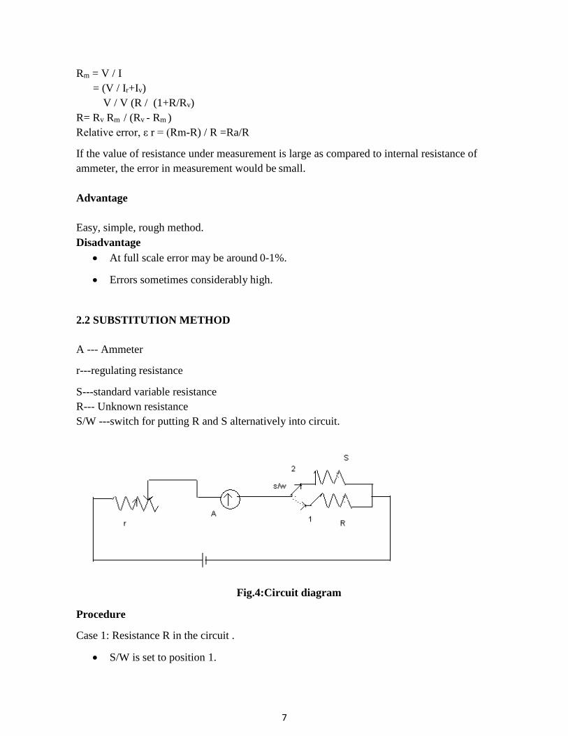
7

Rm = V / I

= (V / Ir+Iv)

V / V (R / (1+R/Rv)

R= Rv Rm / (Rv - Rm )

Relative error, ε r = (Rm-R) / R =Ra/R

If the value of resistance under measurement is large as compared to internal resistance of

ammeter, the error in measurement would be small.

Advantage

Easy, simple, rough method.

Disadvantage

At full scale error may be around 0-1%.

Errors sometimes considerably high.

2.2 SUBSTITUTION METHOD

A --- Ammeter

r---regulating resistance

S---standard variable resistance

R--- Unknown resistance

S/W ---switch for putting R and S alternatively into circuit.

Fig.4:Circuit diagram

Procedure

Case 1: Resistance R in the circuit .

S/W is set to position 1.

8

This brings R into the circuit.

r is adjusted to give ammeter the chosen scale mark.

Case 2: Resistance S in the circuit.

Change S/W to position 2.

This brings S in to the circuit.

Adjust S to give same chosen scale mark by ammeter.

The substitution for one resistance by another has left current unaltered.

The value of S gives the value of R.

Advantage

More accurate than ammeter voltmeter method as no error as the case of ammeter

voltmeter method.

Many applications in bridge method.

Used in high frequency ac measurement.

Disadvantage

Accuracy depends upon constancy of battery emf and resistance of circuit ( excluding

R & S)

Also depends upon accuracy of measurement of S.

2.3 WHEATSTONE BRIDGE

For measuring accurately any electrical resistance Wheatstone bridge is widely used. There are

two known resistors, one variable resistor and one unknown resistor connected in bridge form

as shown below. By adjusting the variable resistor the current through the Galvanometer is

made zero. When the current through the galvanometer becomes zero, the ratio of two known

resistors is exactly equal to the ratio of adjusted value of variable resistance and the value of

unknown resistance. In this way the value of unknown electrical resistance can easily be

measured by using a Wheatstone Bridge.

THEORY

The general arrangement of Wheatstone bridge circuit is shown in the figure below. It is a four

arms bridge circuit where arm AB, BC, CD and AD are consisting of electrical resistances P,

Q, S and R respectively. Among these resistances P and Q are known fixed electrical

resistances and these two arms are referred as ratio arms. An accurate and sensitive

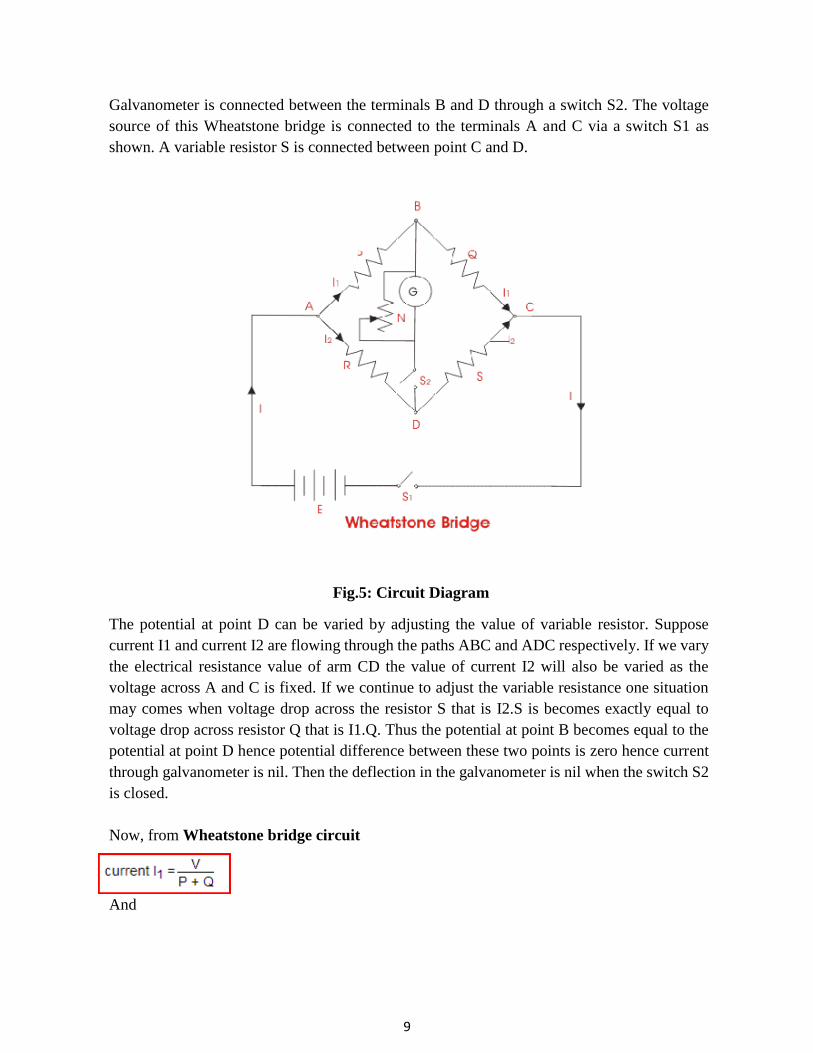
9

Galvanometer is connected between the terminals B and D through a switch S2. The voltage

source of this Wheatstone bridge is connected to the terminals A and C via a switch S1 as

shown. A variable resistor S is connected between point C and D.

Fig.5: Circuit Diagram

The potential at point D can be varied by adjusting the value of variable resistor. Suppose

current I1 and current I2 are flowing through the paths ABC and ADC respectively. If we vary

the electrical resistance value of arm CD the value of current I2 will also be varied as the

voltage across A and C is fixed. If we continue to adjust the variable resistance one situation

may comes when voltage drop across the resistor S that is I2.S is becomes exactly equal to

voltage drop across resistor Q that is I1.Q. Thus the potential at point B becomes equal to the

potential at point D hence potential difference between these two points is zero hence current

through galvanometer is nil. Then the deflection in the galvanometer is nil when the switch S2

is closed.

Now, from Wheatstone bridge circuit

And

10

Now potential of point B in respect of point C is nothing but the voltage drop across the

resistor Q and this is

Again potential of point D in respect of point C is nothing but the voltage drop across the

resistor S and this is

Equating, equations (i) and (ii) we get,

3. MEASUREMENT OF HIGH RESISTANCE

There are different methods that can be employed for the measurement of high

resistances. Some of the important methods are as follows.

i) Direct deflection method

ii) Loss of charge method

iii) Megohm bridge

iv) Megger

3.1 Direct Deflection Method

In this method, a high resistance (more than 1000 Cl) and very sensitive moving coil

galvanometer is connected in series with the resistances to be measured along with supply

voltage as shown in the Figure 1.

11

Fig.6 Direct Deflection

The direct deflection method is used for very high resistances such as insulation

resistances cables. A sensitive galvanometer is used in place of micro ammeter.

The Figure 1shows this method making use of with and without Guard wire at the

terminal A . The Galvanometer G measures the current Ig between the conductor and the metal

sheath. The leakage current IL is actually carried out by the guard wire which ultimately do

not flow through the galvanometer and thereby eliminating the source of error.

Cables without the metal sheaths can be tested in similar way but the cable is immersed

in water tank first except its end where connections are made. The cable should be immersed

for at least 24 hours in slightly alkaline water at a room temperature (approx. 20˚) which will

provide return path for the current as in Figure .The readings obtained give the Volume

resistance of the conductor. The insulation resistance of the cable is given by,

In some cases, the deflection of the galvanometer is observed and its scale is afterwards

calibrated by replacing the insulation by a standard high resistance (usually 1MΩ), the

galvanometer shunt being varied, as required to give a deflection on the same order as before.

In tests on cable the galvanometer should be short-circuited before applying the voltage.

The short-circuiting connection is removed only after sufficient time is elapsed so that charging

and absorption currents cases to flow. The galvanometer should be well shunted during the

early stages of measurement, and it is normally desirable to influence a protective series

resistance (of several megaohm) in the galvanometer circuit. The value of this resistance should

be subtracted from the observed resistance value in order to determine the true resistance. A

high voltage battery of 500V emf is required and its emf should remain constant throughout

the test.

Fig.7 Experimental Diagram

12

3.2 Loss of charge method

In loss of charge method unknown resistance is connected in parallel with capacitor

and electrostatic voltmeter. The capacitor is initially charged to some suitable voltage by means

of a battery of voltage V and then allowed to discharge through the resistance. The terminal

voltage is observed during discharge and it is given by,

V= v exp (-

t/CR) V/v =

exp (-t/CR)

Or insulation resistance is given by,

R= t/(C ln V/v)

= 0.4343 t / (C log V/v)

Fig.8 Circuit Diagram

Fig.9 Volatge vs Time

From above equation it follows that if V, v, C and t are known the value of R can be

computed.If the resistance R is very large the time for an appreciable fall in voltage is very

large and thus this process may become time consuming. Also the voltage-time curve will thus

be very flat and unless great care is taken in measuring voltages at the beginning and at the end

of time t, a serious error may be made in the ratio V/v causing the considerable corresponding

error in the measured value of R. more accurate results may be obtained by change in the

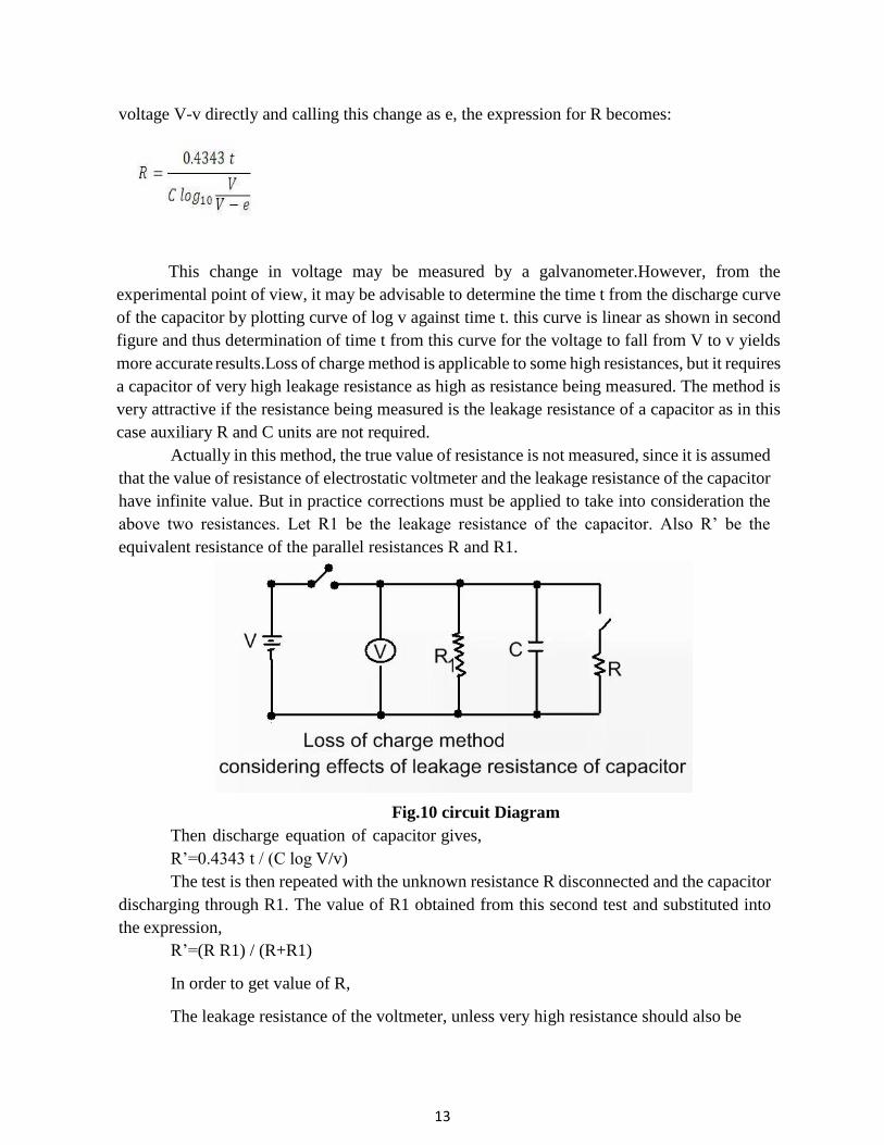
13

voltage V-v directly and calling this change as e, the expression for R becomes:

This change in voltage may be measured by a galvanometer.However, from the

experimental point of view, it may be advisable to determine the time t from the discharge curve

of the capacitor by plotting curve of log v against time t. this curve is linear as shown in second

figure and thus determination of time t from this curve for the voltage to fall from V to v yields

more accurate results.Loss of charge method is applicable to some high resistances, but it requires

a capacitor of very high leakage resistance as high as resistance being measured. The method is

very attractive if the resistance being measured is the leakage resistance of a capacitor as in this

case auxiliary R and C units are not required.

Actually in this method, the true value of resistance is not measured, since it is assumed

that the value of resistance of electrostatic voltmeter and the leakage resistance of the capacitor

have infinite value. But in practice corrections must be applied to take into consideration the

above two resistances. Let R1 be the leakage resistance of the capacitor. Also R’ be the

equivalent resistance of the parallel resistances R and R1.

Fig.10 circuit Diagram

Then discharge equation of capacitor gives,

R’=0.4343 t / (C log V/v)

The test is then repeated with the unknown resistance R disconnected and the capacitor

discharging through R1. The value of R1 obtained from this second test and substituted into

the expression,

R’=(R R1) / (R+R1)

In order to get value of R,

The leakage resistance of the voltmeter, unless very high resistance should also be

14

taken into consideration.

3.3 Megohm bridge

Megohm bridge is another important method for measurement of

high resistances. It has one three terminal high resistance located in one arm of the bridge.

Figure shows the very high resistance with terminals A and B, and a guard terminal, which is

put on the insulation. So it forms a three terminal resistance.

Fig.11 circuit Diagram

Let us consider take the hypothetical case of a 100 Mohm resistance and assume that

this resistance is measured by an ordinary Wheatstone bridge. It is clear that Wheatstone will

measure a resistance of 100*200/(100+200)=67Mohm instead of 100Mohm thus the error is

33 percent.

Fig.12 Wheatstone Bridge

15

However if the same resistance is measured by a modified Wheatstone bridge as shown

in fig b)with the guard connection G connected as indicated, the error in measurement will be

redused and this modified Wheatstone bridge is called megohm bridge.

The arrangement of above figure illustrated the operation of Megohm Bridge.

Figure shows the circuit of the completely elf-contained Megohm Bridge which

includes power supplies, bridge members, amplifiers, and indicating instrument. It has range

from 0.1MΩ to 10^6MΩ. The accuracy is within 3% for the lower part of the range to possible

10% above 10000MΩ.

Sensitivity of balancing against high resistance is obtained by using an adjustable high

voltage supplies of 500V or 1000V and the use of a sensitive null indicating arrangement such

as a high gain amplifier with an electronic voltmeter or a

C.R.O. The dial on Q is calibrated 1-10-100-1000 MΩ, with main decade 1-10 occupying

grater part of the dial space. Since unknown resistance R=PS/Q, the arm Q

is made, tapered, so that the dial calibration is approximately logarithmic in the main decade,

1-10. Arm S give five multipliers, 0.1,1,10,100 and 1000.

3.4 MEGGER

1) Deflecting & Control coil : Connected parallel to the generator, mounted at right angle to

each other and maintain polarities in such a way to produced torque in opposite direction.

2) Permanent Magnets: Produce magnetic field to deflect pointer with North-South pole

magnet.

3) Pointer : One end of the pointer connected with coil another end deflects on scale from

infinity to zero.

4) Scale : A scale is provided in front-top of the megger from range ‘zero’ to ‘infinity’, enable

us to read the value.

5) D.C generator or Battery connection : Testing voltage is produced by hand operated D.C

generator for manual operated Megger. Battery / electronic voltage charger is provided for

automatic type Megger for same purpose.

6) Pressure coil resistance and Current coil resistance : Protect instrument from any damage

because of low external electrical resistance under test.

16

Fig.13 Megger

Working Principle of Megger

• Voltage for testing produced by hand operated Megger by rotation of crank in case of hand

operated type, a battery is used for electronic tester.

• 500 Volt DC is sufficient for performing test on equipment range up to 440 Volts.

• 1000V to 5000V is used for testing for high voltage electrical systems.

• Deflecting coil or current coil connected in series and allows flowing the electric current

taken by the circuit being tested.

• The control coil also known as pressure coil is connected across the circuit. Current limiting

resistor (CCR & PCR ) connected in series with control & deflecting coil to protect damage in

case of very low resistance in external circuit.

• In hand operated megger electromagnetic induction effect is used to produce the test voltage

i.e. armature arranges to move in permanent magnetic field or vice versa.

• Where as in electronic type megger battery are used to produce the testing voltage.

• As the voltage increases in external circuit the deflection of pointer increases and deflection

of pointer decreases with a increases of current.

• Hence, resultant torque is directly proportional to voltage & inversely proportional to current.

• When electrical circuit being tested is open, torque due to voltage coil will be maximum &

pointer shows ‘infinity’ means no shorting throughout the circuit and has maximum resistance

within the circuit under test.

• If there is short circuit pointer shows ‘zero’, which means ‘NO’ resistance within circuit

being tested.

Work philosophy based on ohm-meter or ratio-meter. The deflection torque is produced with

17

megger tester due to the magnetic field produced by voltage & current, similarly like ‘Ohm's

Law’ Torque of the megger varies in ration with V/I, (Ohm's Law :- V=IR or R=V/I).

Electrical resistance to be measured is connected across the generator & in series with

deflecting coil. Produced torque shall be in opposite direction if current supplied to the coil.

1. High resistance = No current :- No current shall flow through deflecting coil, if resistance

is very high i.e. infinity position of pointer

2. Small resistance = High current :- If circuit measures small resistance allows a high

electric current to pass through deflecting coil, i.e. produced torque make the pointer to set at

‘ZERO’.

3. Intermediate resistance = varied current :- If measured resistance is intermediate,

produced torque align or set the pointer between the range of ‘ZERO to INIFINITY’

Maxwell’s inductance bridge

The choke for which R1 and L1 have to measure connected between the points ‘A’ and

‘B’. In this method the unknown inductance is measured by comparing it with the standard

inductance.

L2 is adjusted, until the detector indicates zero current.

Let R1=unknown resistance

L1= unknown

L2 is adjusted, until the detector indicates zero current.

Let R1= unknown resistance

L1= unknown inductance of the choke.

L2= known standard inductance

R1,R2,R4= known resistances

Fig 14 Circuit Diagram

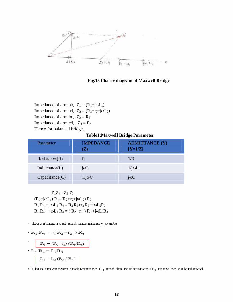
18

Fig.15 Phasor diagram of Maxwell Bridge

Impedance of arm ab, Z1 = (R1+jωL1)

Impedance of arm ad, Z2 = (R2+r2+jωL2)

Impedance of arm bc, Z3 = R3

Impedance of arm cd, Z4 = R4

Hence for balanced bridge,

Table1:Maxwell Bridge Parameter

Parameter IMPEDANCE

(Z)

ADMITTANCE (Y)

[Y=1/Z]

Resistance(R) R 1/R

Inductance(L) jωL 1/jωL

Capacitance(C) 1/jωC jωC

Z1Z4 =Z2 Z3

(R1+jωL1) R4=(R2+r2+jωL2) R3

R1 R4 + jωL1 R4 = R2 R3+r2 R3 +jωL2R3

R1 R4 + jωL1 R4 = ( R2 +r2 ) R3 +jωL2R3

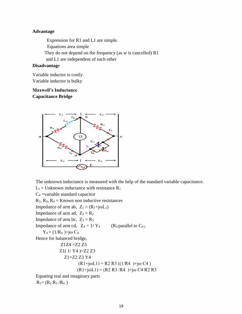
19

Advantage

Expression for R1 and L1 are simple.

Equations area simple

They do not depend on the frequency (as w is cancelled) R1

and L1 are independent of each other

Disadvantage

Variable inductor is costly.

Variable inductor is bulky

Maxwell’s Inductance

Capacitance Bridge

The unknown inductance is measured with the help of the standard variable capacitance.

L1 = Unknown inductance with resistance R1

C4 =variable standard capacitor

R2, R3, R4 = Known non inductive resistances

Impedance of arm ab, Z1 = (R1+jωL1)

Impedance of arm ad, Z2 = R2

Impedance of arm bc, Z3 = R3

Impedance of arm cd, Z4 = 1/ Y4 (R4 parallel to C4 )

Y4 = (1/R4 )+jω C4

Hence for balanced bridge,

Z1Z4 =Z2 Z3

Z1( 1/ Y4 )=Z2 Z3

Z1=Z2 Z3 Y4

(R1+jωL1) = R2 R3 ((1/R4 )+jω C4 )

(R1+jωL1) = (R2 R3 /R4 )+jω C4 R2 R3

Equating real and imaginary parts

R1= (R2 R3 /R4 )

20

L1= C4 R2 R3

Thus unknown inductance L1 and its resistance R1 may be calculated

Table2: Maxwell Capacitance Bridge

Parameter IMPEDANCE (Z) ADMITTANCE (Y)

[Y=1/Z]

Resistance(R) R 1/R

Inductance(L) jωL 1/jωL

Capacitance(C) 1/jωC jωC

HAY’S BRIDGE

Hay's bridge is modified Maxwell bridge, now question arises here in our mind that where we

need to do modification.

• The Hay’s bridge is used for determining the self-inductance of the circuit.

• The bridge is the advanced form of Maxwell’s bridge.

• The Maxwell’s bridge is only appropriate for measuring the medium quality factor.

• Hence, for measuring the high-quality factor the Hays bridge is used in the circuit.

• In Hay’s bridge, the capacitor is connected in series with the resistance, the voltage

drop across the capacitance and resistance are varied.

• And in Maxwell bridge, the capacitance is connected in parallel with the resistance.

• Thus, the magnitude of a voltage pass through the resistance and capacitor is equal.

Fig .16 Hays Bridge

The unknown inductor L1 is placed in the arm ab along with the resistance R1. This unknown

inductor is compared with the standard capacitor C4 connected across the arm cd. The

resistance R4 is connected in series with the capacitor C4. The other two non-inductive

resistor R2 and R3 are connected in the arm ad and bc respectively. The C4 and R4 are

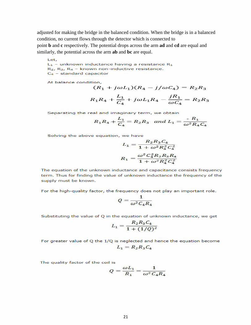
21

adjusted for making the bridge in the balanced condition. When the bridge is in a balanced

condition, no current flows through the detector which is connected to

point b and c respectively. The potential drops across the arm ad and cd are equal and

similarly, the potential across the arm ab and bc are equal.

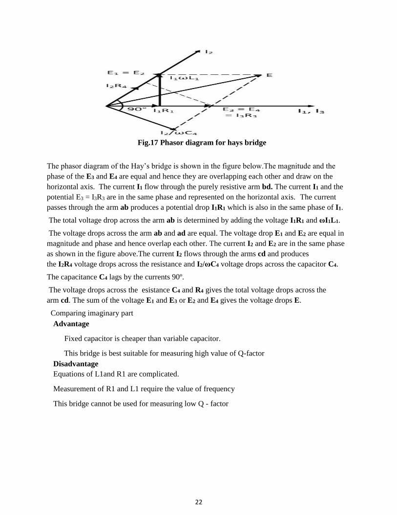
22

Fig.17 Phasor diagram for hays bridge

The phasor diagram of the Hay’s bridge is shown in the figure below.The magnitude and the

phase of the E3 and E4 are equal and hence they are overlapping each other and draw on the

horizontal axis. The current I1 flow through the purely resistive arm bd. The current I1 and the

potential E3 = I3R3 are in the same phase and represented on the horizontal axis. The current

passes through the arm ab produces a potential drop I1R1 which is also in the same phase of I1.

The total voltage drop across the arm ab is determined by adding the voltage I1R1 and ωI1L1.

The voltage drops across the arm ab and ad are equal. The voltage drop E1 and E2 are equal in

magnitude and phase and hence overlap each other. The current I2 and E2 are in the same phase

as shown in the figure above.The current I2 flows through the arms cd and produces

the I2R4 voltage drops across the resistance and I2/ωC4 voltage drops across the capacitor C4.

The capacitance C4 lags by the currents 90º.

The voltage drops across the esistance C4 and R4 gives the total voltage drops across the

arm cd. The sum of the voltage E1 and E3 or E2 and E4 gives the voltage drops E.

Comparing imaginary part

Advantage

Fixed capacitor is cheaper than variable capacitor.

This bridge is best suitable for measuring high value of Q-factor

Disadvantage

Equations of L1and R1 are complicated.

Measurement of R1 and L1 require the value of frequency

This bridge cannot be used for measuring low Q - factor

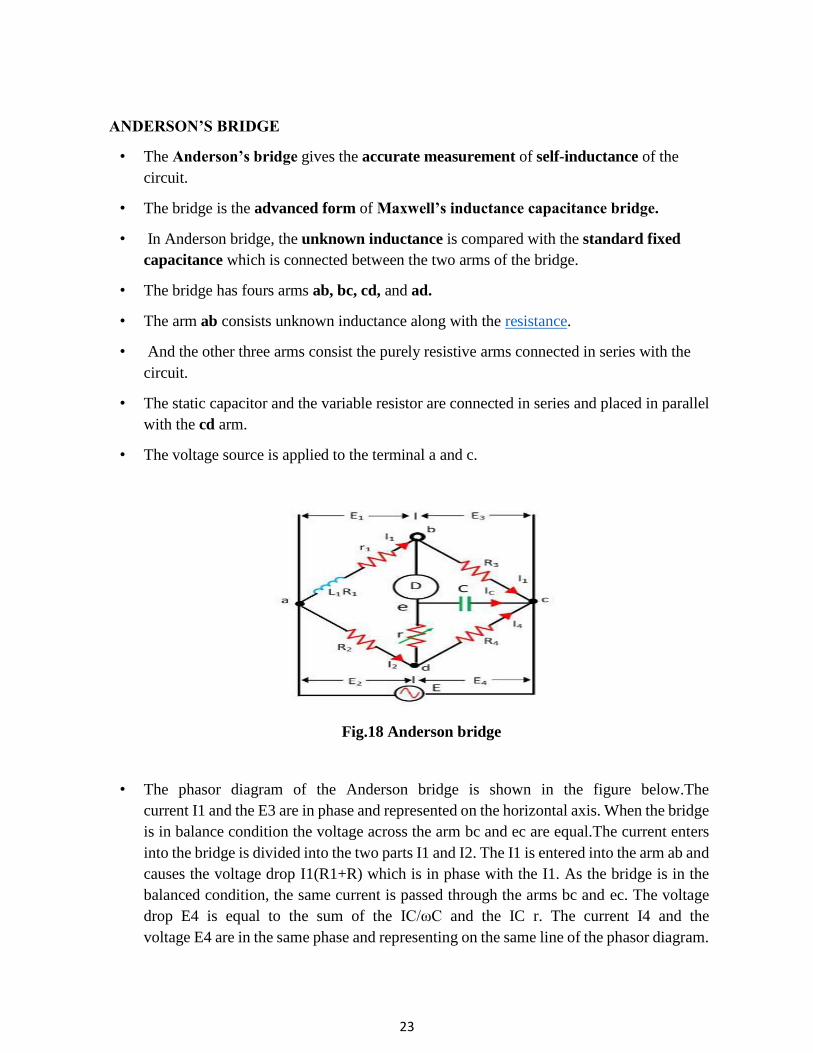
23

ANDERSON’S BRIDGE

• The Anderson’s bridge gives the accurate measurement of self-inductance of the

circuit.

• The bridge is the advanced form of Maxwell’s inductance capacitance bridge.

• In Anderson bridge, the unknown inductance is compared with the standard fixed

capacitance which is connected between the two arms of the bridge.

• The bridge has fours arms ab, bc, cd, and ad.

• The arm ab consists unknown inductance along with the resistance.

• And the other three arms consist the purely resistive arms connected in series with the

circuit.

• The static capacitor and the variable resistor are connected in series and placed in parallel

with the cd arm.

• The voltage source is applied to the terminal a and c.

Fig.18 Anderson bridge

• The phasor diagram of the Anderson bridge is shown in the figure below.The

current I1 and the E3 are in phase and represented on the horizontal axis. When the bridge

is in balance condition the voltage across the arm bc and ec are equal.The current enters

into the bridge is divided into the two parts I1 and I2. The I1 is entered into the arm ab and

causes the voltage drop I1(R1+R) which is in phase with the I1. As the bridge is in the

balanced condition, the same current is passed through the arms bc and ec. The voltage

drop E4 is equal to the sum of the IC/ωC and the IC r. The current I4 and the

voltage E4 are in the same phase and representing on the same line of the phasor diagram.

24

The sum of the current IC and I4 will give rise to the current I2 in the arm ad.When the

bridge is at balance condition the emf across the arm ab and the point a, d and e are equal.

The phasor sum of the voltage across the arms ac and de will give rise the voltage drops

across the arm ab.The V1 is also obtained by adding the I1(R1+r1) with the voltage

drop ωI1L1 in the arm AB. The phasor sum of the E1 and E3 or E2 and E4 will give the

supply voltage. Let, L1: unknown inductance having a resistance .R1,R2,R3,R3-know

non inductive resistance

The above equation obtained is more complex that we have obtained in Maxwell bridge. On

observing the above equations we can easily say that to obtain convergence of balance more

easily, one should make alternate adjustments of r1 and r in Anderson’s bridge. Now let us

look how we can obtain the value of unknown inductor experimentally. At first set the signal

generator frequency at audible range. Now adjust r1 and r such that phones gives a minimum

sound. Measure the values of r1 and r (obtained after these adjustments) with the help of

multimeter. Use the formula that we have derived above in order to find out the value of

25

unknown inductance. The experiment can be repeated with the different value of standard

capacitor.

Phasor Diagram of Anderson's Bridge

Let us mark the voltage drops across ab, bc, cd and ad as e1, e2, e3 and e4 as shown

Fig .19 Phasor Diagram

Here in the phasor diagram of Anderson's bridge, we have taken i1 as reference axis. Now ic

is perpendicular to i1 as capacitive load is connected at ec, i4 and i2 are lead by some angle as

shown in figure. Now the sum of all the resultant voltage drops i.e. e1, e2, e3 and e4 is equal

to e, which is shown in phasor diagram. As shown in the phasor diagram of Anderson's bridge

the resultant of voltages drop i1

(R1 + r1) and i1.ω.l1 (which is shown perpendicular to i1) is e1. e2 is given by i2.r2 which

makes angle 'A' with the reference axis. Similarly, e4 can be obtained by voltage drop i4.r4

which is making angle 'B' with reference axis.

Advantages of Anderson's Bridge

1. It is very easy to obtain the balance point in Anderson's bridge as compared to Maxwell

bridge in case of low quality factor coils.

2. There is no need of variable standard capacitor is required instead of thin a fixed value

capacitor is used.

3. This bridge also gives accurate result for determination of capacitance in terms of

inductance.

Disadvantages of Anderson's Bridge

1. The equations obtained for inductor in this bridge is more complex as complex as

compared to Maxwell's bridge.

2. The addition of capacitor junction increases complexity as well as difficulty of shielding

the bridge.

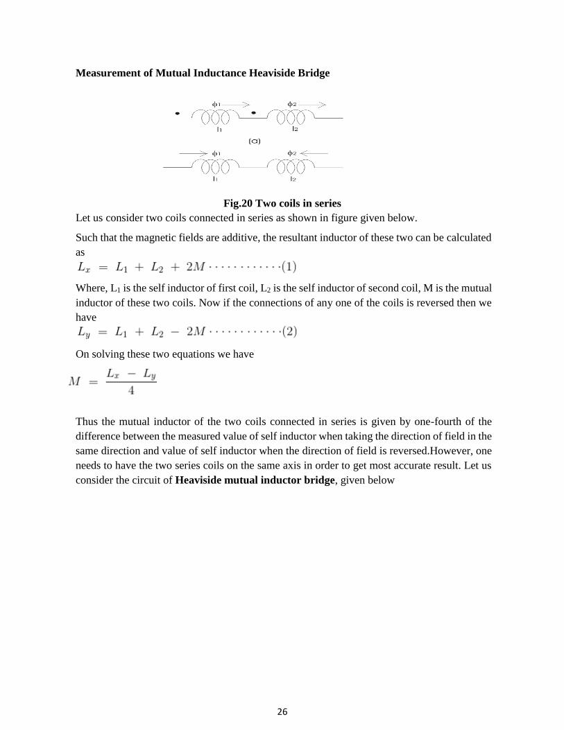
26

Measurement of Mutual Inductance Heaviside Bridge

Fig.20 Two coils in series

Let us consider two coils connected in series as shown in figure given below.

Such that the magnetic fields are additive, the resultant inductor of these two can be calculated

as

Where, L1 is the self inductor of first coil, L2 is the self inductor of second coil, M is the mutual

inductor of these two coils. Now if the connections of any one of the coils is reversed then we

have

On solving these two equations we have

Thus the mutual inductor of the two coils connected in series is given by one-fourth of the

difference between the measured value of self inductor when taking the direction of field in the

same direction and value of self inductor when the direction of field is reversed.However, one

needs to have the two series coils on the same axis in order to get most accurate result. Let us

consider the circuit of Heaviside mutual inductor bridge, given below

27

Fig.21 Heavy side Mutual Inductance Bridge

Main application of this bridge in industries is to measure the mutual inductor in terms of self

inductance. Circuit of this bridge consists of four non inductive resistors r1, r2, r3 and r4

connected on arms 1-2, 2-3, 3-4 and 4-1 respectively. In series of this bridge circuit an unknown

mutual inductor is connected. A voltage is applied to across terminals 1 and 3. At balance point

electric current flows through 2-4 is zero hence the voltage drop across 2-3 is equal to voltage

drop across 4-3. So by equating the voltage drops of 2-4 and 4-3 we have,

Also we have,

and mutual inductor is given by,

28

Measurement of Capacitance Schering Bridge

This bridge is used to measure to the capacitance of the capacitor, dissipation factor and

measurement of relative permittivity. Let us consider the circuit of Schering bridge

Fig.22 Schering Bridge

Here, c1 is the unknown capacitance whose value is to be determined with series electrical

resistance r1. c2 is a standard capacitor. c4 is a variable capacitor. r3 is a pure resistor (i.e. non

inductive in nature). And r4 is a variable non inductive resistor connected in parallel with

variable capacitor c4. Now the supply is given to the bridge between the points a and c.

The detector is connected between b and d. From the theory of ac bridges we have at balance

condition,

Substituting the values of z1, z2, z3 and z4 in the above equation, we get

Equating the real and imaginary parts and the separating we get,

29

Fig.23 Phasor Diagram

consider the phasor diagram of the above Shering bridge circuit and mark the voltage drops

across ab,bc,cd and ad as e1, e3,e4 and e2 respectively. From the above Schering bridge phasor

diagram, we can calculate the value of tanδ which is also called the dissipation factor.

DE SAUTY’S BRIDGE

This bridge provide us the most suitable method for comparing the two values of capacitor if

we neglect dielectric losses in the bridge circuit. The circuit of De Sauty's bridge is shown.

Fig.24 Sauty Bridge

Battery is applied between terminals marked as 1 and 4. The arm 1-2 consists of capacitor c1

30

(whose value is unknown) which carries current i1 as shown, arm 2 - 4 consists of pure resistor

(here pure resistor means we assuming it non inductive in nature), arm 3 - 4 also consists of

pure resistor and arm 4 - 1 consists of standard capacitor whose value is already known to us.

Let us derive the expression for capacitor c1 in terms of standard capacitor and resistors.

At balance condition we have,

It implies that the value of capacitor is given by the expression

In order to obtain the balance point we must adjust the values of either r3 or r4 without disturbing

any other element of the bridge. This is the most efficient method of comparing the two values

of capacitor if all the dielectric losses are neglected from the circuit.

Fig .24 Phasor diagram of De Sauty bridge

Now instead of some advantages like bridge is quite simple and provides easy calculations,

there are some disadvantages of this bridge because this bridge give inaccurate results for

imperfect capacitor (here imperfect means capacitors which not free from dielectric losses).

Hence we can use this bridge only for comparing perfect capacitors. Here we interested in

modify the De Sauty's bridge, we want to have such a kind of bridge that will gives us accurate

results for imperfect capacitors also.

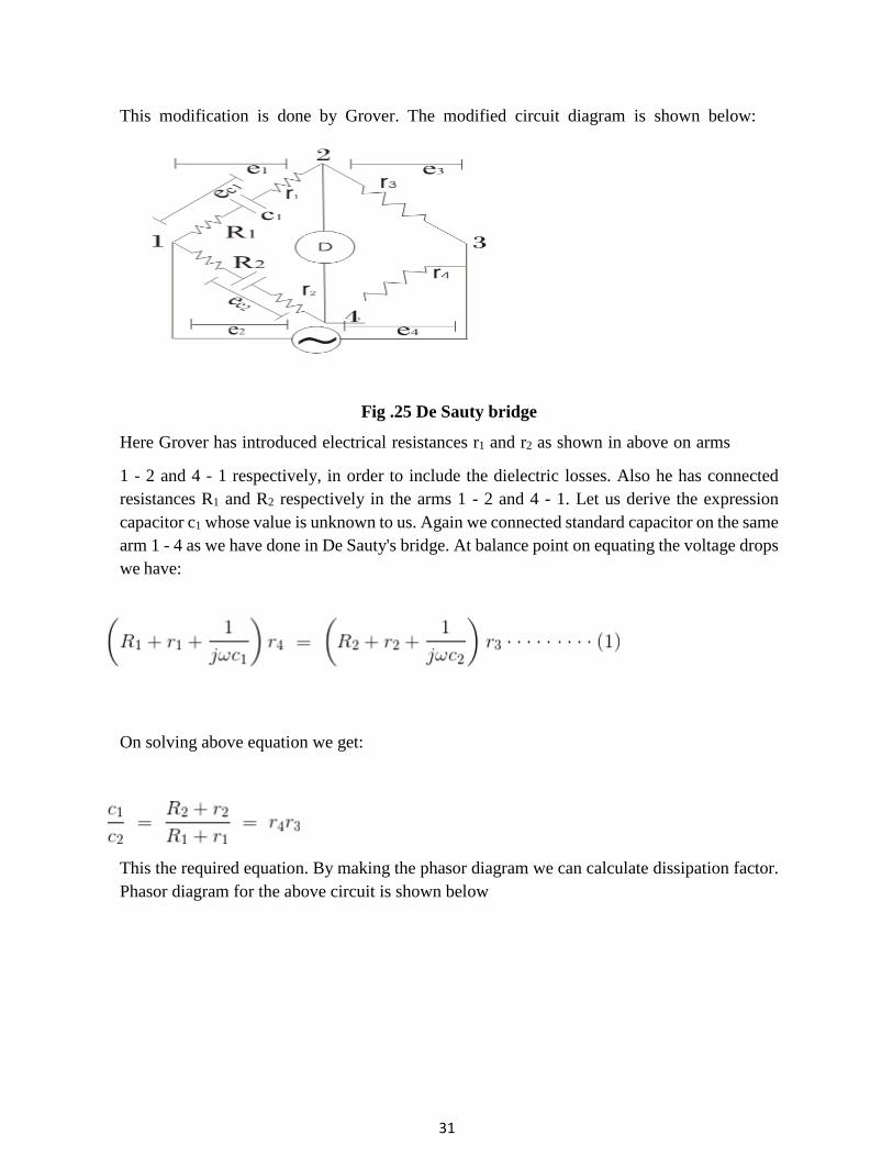
31

This modification is done by Grover. The modified circuit diagram is shown below:

Fig .25 De Sauty bridge

Here Grover has introduced electrical resistances r1 and r2 as shown in above on arms

1 - 2 and 4 - 1 respectively, in order to include the dielectric losses. Also he has connected

resistances R1 and R2 respectively in the arms 1 - 2 and 4 - 1. Let us derive the expression

capacitor c1 whose value is unknown to us. Again we connected standard capacitor on the same

arm 1 - 4 as we have done in De Sauty's bridge. At balance point on equating the voltage drops

we have:

On solving above equation we get:

This the required equation. By making the phasor diagram we can calculate dissipation factor.

Phasor diagram for the above circuit is shown below

32

Fig.26 Phasor Diagram

Let us mark δ1 and δ2 be phase angles of the capacitors c1 and c2 capacitors respectively. From

the phasor diagram we have tan(δ1) = dissipation factor = ωc1r1 and similarly we have tan(δ2)

= ωc2r2. From equation (1) we have

on multiplying ω both sides we have

Therefore the final expression for the dissipation factor is written as

Hence if dissipation factor for one capacitor is known. However this method is gives quite

inaccurate results for dissipation factor.

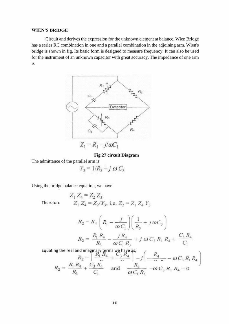
33

WIEN’S BRIDGE

Circuit and derives the expression for the unknown element at balance, Wien Bridge

has a series RC combination in one and a parallel combination in the adjoining arm. Wien's

bridge is shown in fig. Its basic form is designed to measure frequency. It can also be used

for the instrument of an unknown capacitor with great accuracy, The impedance of one arm

is

Fig.27 circuit Diagram

The admittance of the parallel arm is

Using the bridge balance equation, we have

Therefore

Equating the real and imaginary terms we have as,

34

The bridge is used for measuring frequency in the audio range. Resistances R1 and R3 can

be ganged together to have identical values. Capacitors C1 and C3 are normally of fixed

values. The audio range is normally divided into 20 - 200 - 2 k - 20 kHz range In this case,

the resistances can be used for range changing and capacitors, and C3 for fine frequency

control within the range. The bridge can also be use for measuring capacitance. In that case,

the frequency of operation must be known.

The bridge is also used in a harmonic distortion analyzer, as a Notch filter, an in audio

frequency and radio frequency oscillators as a frequency determine element.

An accuracy of 0.5% - 1% can be readily obtained using this bridge. Because it is frequency

sensitive, it is difficult to balance unless the waveform of the applied voltage is purely

sinusoidal.

Reference books

1. Sawhney A.K., “A Course in Electrical, Electronic measurement &

Instrumentation”, Dhanpat Rai & sons, 18th Edition, Reprint 2010.

2. Doebelin E.O., “Measurement System Applications and Design”, McGraw Hill,

5th Edition, 2004.

3. Jain R.K., “Mechanical and Industrial Measurements”, Khanna Publishers, 11th

edition, Reprint 2005.

4. Jones’ Instrument Technology, Instrumentation Systems, Edited by B.E.Noltingk,

Vol 4, 4th edition, ELBS, 1987.

5. Murthy D.V.S., “Transducers and Instrumentation”, Printice Hall of India, 13th

printing, 2006.

6. Gnanavadivel,“Measurements and Instrumentation”,Anuradha Publication, Second

35

Revised Edition 2011.

SCHOOL OF ELECTRICAL AND ELECTRONICS

DEPARTMENT OF ELECTRONICS AND INSTRUMENTATION

UNIT – IV

MEASUREMENT AND INSTRUMENTATION – SIC 1203

UNIT-4

ELECTRONIC MEASUREMENTS

Fundamentals of Cathode Ray Oscilloscope: Block diagram, CRO probes, Delay line,

types of Oscilloscopes. Measurement of: Signal voltage, Current, Phase & Frequency

using Lissajous patterns, Industrial applications of CRO. DC and AC voltmeter and

Ammeter, Ohmmeter, Range Extension, Electronic Multimeters, Types of Voltmeters -

Differential type, true RMS type, Vector voltmeter - Wave Analyzer, Spectrum Analyzer

and Distortion Analyzer

1. INTRODUCTION- CATHODE RAY TUBE (CRT)

In studying the various electronic, electrical networks and systems, signals which are

functions of time, are often encountered. Such signals may be periodic or non-periodic in nature.

The device which allows, the amplitude of such signals, to be displayed primarily as a function of

time, is called cathode ray oscilloscope, commonly known as C.R.O. The C.R.O. gives the visual

representation of the time varying signals. The oscilloscope has become an universal instrument

and is probably most versatile tool for the development of electronic circuits and systems. It is an

integral part of electronic laboratories.

The oscilloscope is, in fact, a voltmeter. Instead of the mechanical deflection of a metallic

pointer as used in the normal voltmeters, the oscilloscope uses the movement of an electron beam

against a fluorescent screen, which produces the movement of a visible spot. The movement of

such spot on the screen is proportional to the varying magnitude of the signal, which is under

measurement.

The electron beam can be deflected in two directions: the horizontal or x-direction and the

vertical or y-direction. Thus an electron beam producing a spot can be used to produce two

dimensional displays. Thus C.R.O. can be regarded as a fast x-y plotter. The X-axis and y-axis can

be used to study the variation of one voltage as a function of another. Typically the x-axis of the

oscilloscope represents the time while the y-axis represents variation of the input voltage signal.

Thus if the input voltage signal applied to the y-axis of C.R.O. is sinusoidal varying and if x-axis

represents the time axis, then the spot moves sinusoidal, and the familiar sinusoidal waveform can

be seen on the screen of the oscilloscope. The oscilloscope is so fast device that it can display the

periodic signals whose time period is as small as microseconds and even nanoseconds. The C.R.O.

basically operates on voltages, but it is possible to convert current, pressure, strain, acceleration

and other physical quantities into the voltage using transducers and obtain their visual

representations on the C.R.O.

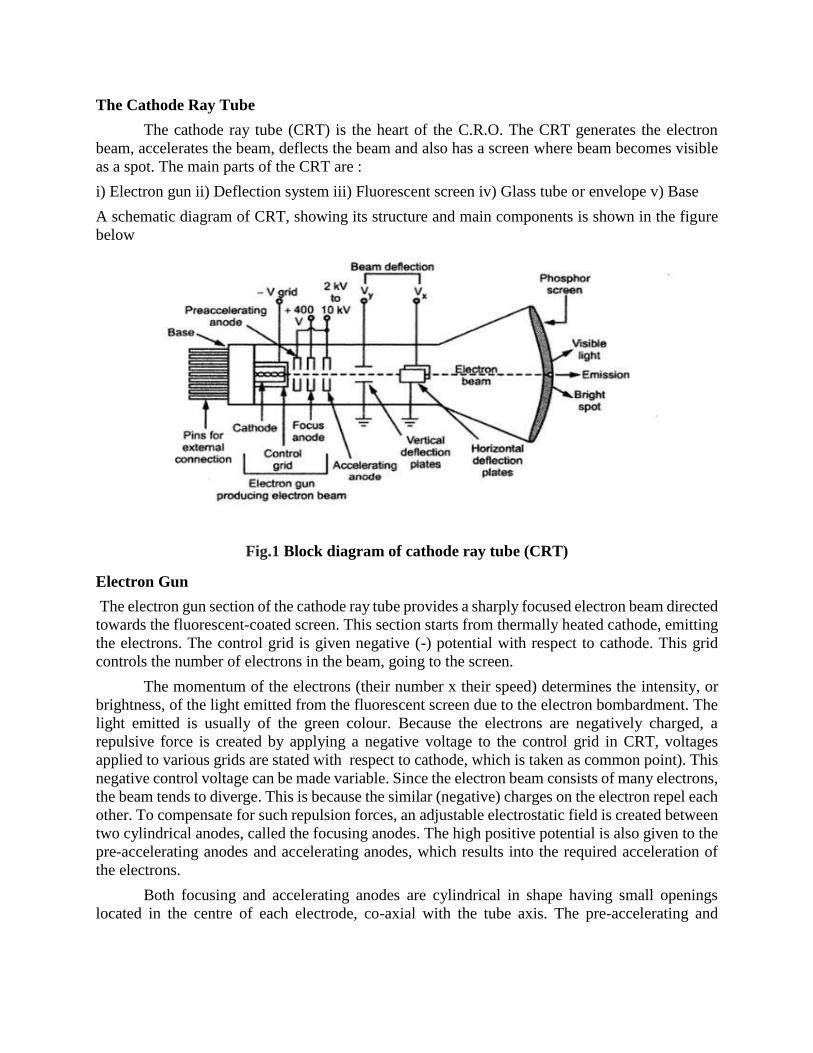
The Cathode Ray Tube

The cathode ray tube (CRT) is the heart of the C.R.O. The CRT generates the electron

beam, accelerates the beam, deflects the beam and also has a screen where beam becomes visible

as a spot. The main parts of the CRT are :

i) Electron gun ii) Deflection system iii) Fluorescent screen iv) Glass tube or envelope v) Base

A schematic diagram of CRT, showing its structure and main components is shown in the figure

below

Fig.1 Block diagram of cathode ray tube (CRT)

Electron Gun

The electron gun section of the cathode ray tube provides a sharply focused electron beam directed

towards the fluorescent-coated screen. This section starts from thermally heated cathode, emitting

the electrons. The control grid is given negative (-) potential with respect to cathode. This grid

controls the number of electrons in the beam, going to the screen.

The momentum of the electrons (their number x their speed) determines the intensity, or

brightness, of the light emitted from the fluorescent screen due to the electron bombardment. The

light emitted is usually of the green colour. Because the electrons are negatively charged, a

repulsive force is created by applying a negative voltage to the control grid in CRT, voltages

applied to various grids are stated with respect to cathode, which is taken as common point). This

negative control voltage can be made variable. Since the electron beam consists of many electrons,

the beam tends to diverge. This is because the similar (negative) charges on the electron repel each

other. To compensate for such repulsion forces, an adjustable electrostatic field is created between

two cylindrical anodes, called the focusing anodes. The high positive potential is also given to the

pre-accelerating anodes and accelerating anodes, which results into the required acceleration of

the electrons.

Both focusing and accelerating anodes are cylindrical in shape having small openings

located in the centre of each electrode, co-axial with the tube axis. The pre-accelerating and

accelerating anodes are connected to a common positive high voltage which varies between 2 kV

to 10 kV. The focusing anode is connected to a lower positive voltage of about 400 V to 500 V.

Deflection system

When the electron beam is accelerated it passes through the deflection system, with which beam

can be positioned anywhere on the screen. The deflection system of the cathode-ray-tube consists

of two pairs of parallel plates, referred to as the vertical and horizontal deflection plates. One of

the plates in each set is connected to ground 0 V). To the other plate of each set, the external

deflection voltage is applied through an internal adjustable gain amplifier stage. To apply the

deflection voltage externally, an external terminal, called the Y input or the X input, is available.

As shown in the figure above, the electron beam passes through these plates. A positive

voltage applied to the Y input terminal (Vy) causes the beam to deflect vertically upward due to

the attraction forces, while a negative voltage applied to the Y input terminal will cause the electron

beam to deflect vertically downward, due to the repulsion forces.

Similarly, a positive voltage applied to X-input terminal (Vx) will cause the electron beam

to deflect horizontally towards the right; while a negative voltage applied to the X-input terminal

will cause the electron beam to deflect. horizontally towards the left of the screen. The amount of

vertical or horizontal deflection is directly proportional to the correspondingly applied voltage.

When the voltages are applied simultaneously to vertical and horizontal deflecting plates,

the electron beam is deflected due to the resultant of these two voltages. The face of the screen can

be considered as an x-y plane. The (x,y) position of the beam spot is thus directly influenced by

the horizontal and the vertical voltages applied to the deflection plates Vx, and Vy, respectively.

The horizontal deflection (x) produced will be proportional to the horizontal deflecting voltage,

Vx, applied to X-input.

x ∝ V

x = KXVX

where Kx is constant of proportionality. The deflection produced is usually measured in cm or as

number of divisions, on the scale, in the horizontal direction.

Then Kx = x/Vx where Kx is expressed as cm/volt or division/volt, is called horizontal sensitivity

of the oscilloscope.

Similarly, the vertical deflection (y) produced will be proportional to the vertical deflecting

voltage, Vy, applied to the y-input.

y ∝ V

y = KyVy

Then Ky = y/Vy and Ky, the vertical sensitivity, will be expressed as cm/volt, or division/volt.

The values of vertical and horizontal sensitivities are selectable and adjustable through

multipositional switches on the front panel that controls the gain of the corresponding internal

amplifier stage. The bright spot of the electron beam can thus trace (or plot) the x-y relationship

between the two voltages, Vx and Vy.

The schematic arrangement of the vertical and the horizontal plates, controlling the position of the

spot on the screen is shown in the figure below:

Fig.2 Arrangements of Plates in CRT

Fluorescent screen

The light produced by the screen does not disappear immediately when bombardment by electrons

ceases, i.e., when the signal becomes zero. The time period for which the trace remains on the

screen after the signal becomes zero is known as "persistence". The persistence may be as short as

a few microsecond, or as long as tens of seconds or even minutes. Medium persistence traces are

mostly used for general purpose applications. Long persistence traces are used in the study of

transients. Long persistence helps in the study of transients since the trace is still seen on the screen

after the transient has disappeared. Short persistence is needed for extremely high speed

phenomena.

The screen is coated with a fluorescent material called phosphor which emits light when

bombarded by electrons. There are various phosphors available which differ in colour, persistence,

and efficiency.

One of the common phosphor is Willemite, which is zinc, orthosilicate, ZnO+SiO2, with

traces of manganese. This produces the familiar greenish trace. Other useful screen materials

include compounds of zinc, cadmium, magnesium and silicon. The kinetic energy of the electron

beam is converted into both light and heat energy when it hits the screen. The heat so produced

gives rise to "phosphor burn" which is damaging and sometimes destructive. This degrades the

light output of phosphor and sometimes may cause complete phosphor destruction. Thus the

phosphor must have high burn resistance to avoid accidental damage.

Many phosphor materials having different excitation times and colours as well as different

phosphorescence times are available. The type P1, P2, P11 or P31 are the short persistence phosphors

and are used for the general purpose oscilloscopes.

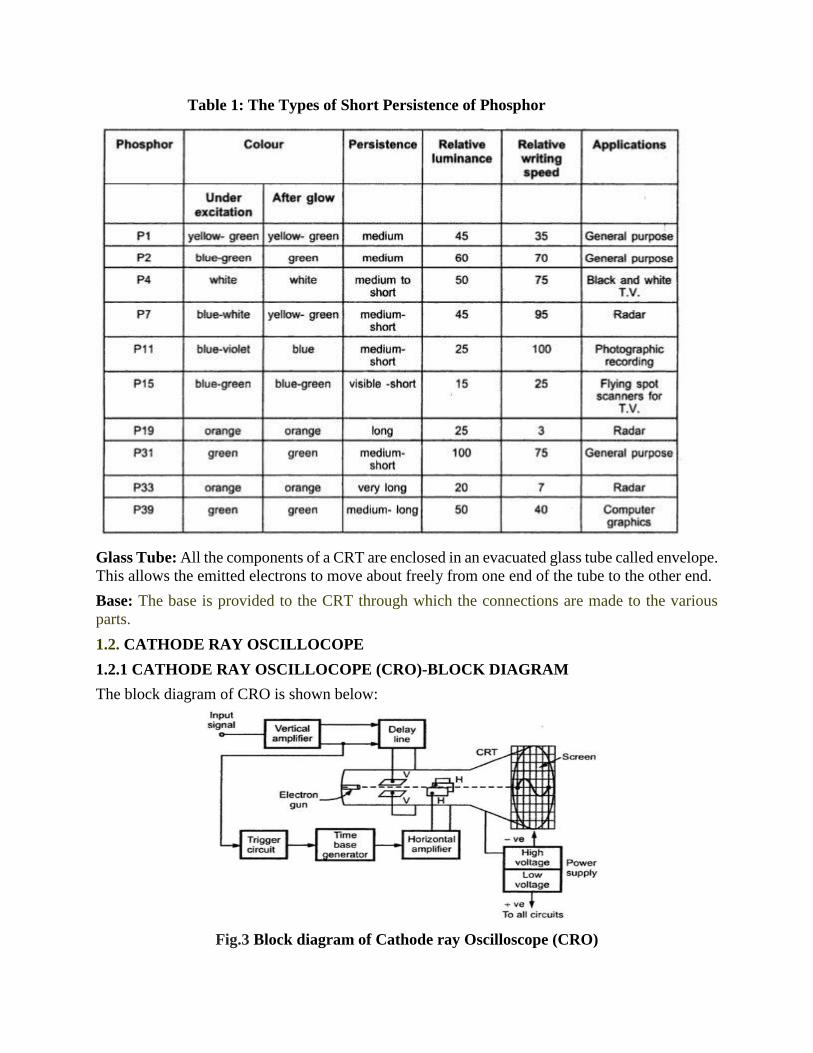
Table 1: The Types of Short Persistence of Phosphor

Glass Tube: All the components of a CRT are enclosed in an evacuated glass tube called envelope.

This allows the emitted electrons to move about freely from one end of the tube to the other end.

Base: The base is provided to the CRT through which the connections are made to the various

parts.

1.2. CATHODE RAY OSCILLOCOPE

1.2.1 CATHODE RAY OSCILLOCOPE (CRO)-BLOCK DIAGRAM

The block diagram of CRO is shown below:

Fig.3 Block diagram of Cathode ray Oscilloscope (CRO)

Cathode Ray Tube (CRT): This is the cathode ray tube which is the heart of C.R.O. It is used to

emit the electrons required to strike the phosphor screen to produce the spot for the visual display

of the signals.

Vertical Amplifier: The input signals are generally not strong to provide the measurable

deflection on the screen. Hence the vertical amplifier stage is used to amplify the input signals.

The amplifier stages used are generally wide band amplifiers so as to pass faithfully the entire

band of frequencies to be measured. Similarly it contains the attenuator stages as well. The

attenuators are used when very high voltage signals are to be examined, to bring the signals within

the proper range of operation.

The block diagram of a vertical amplifier is shown in the figure below.

Fig.4 Vertical amplifier

It consists of several stages with overall fixed sensitivity. The amplifier can be designed

for stability and required bandwidth very easily due to the fixed gain. The input stage consists of

an attenuator followed by FET source follower. It has very high input impedance required to isolate

the amplifier from the attenuator. It is followed by BJT emitter follower to match the output

impedance of FET output with input of phase inverter. The phase inverter provides two anti-phase

output signals which are required to operate the push pull output amplifier.

The push pull operation has advantages like better hum voltage cancellation, even

harmonic suppression especially large and harmonic, greater power output per tube and reduced

number of defocusing and nonlinear effects.

Delay Line: The delay line is used to delay the signal for some time in the vertical sections. When

the delay line is not used, the part of the signal gets lost. Thus the input signal is not applied directly

to the vertical plates but is delayed by some time using a delay line circuit as shown in the figure

below:

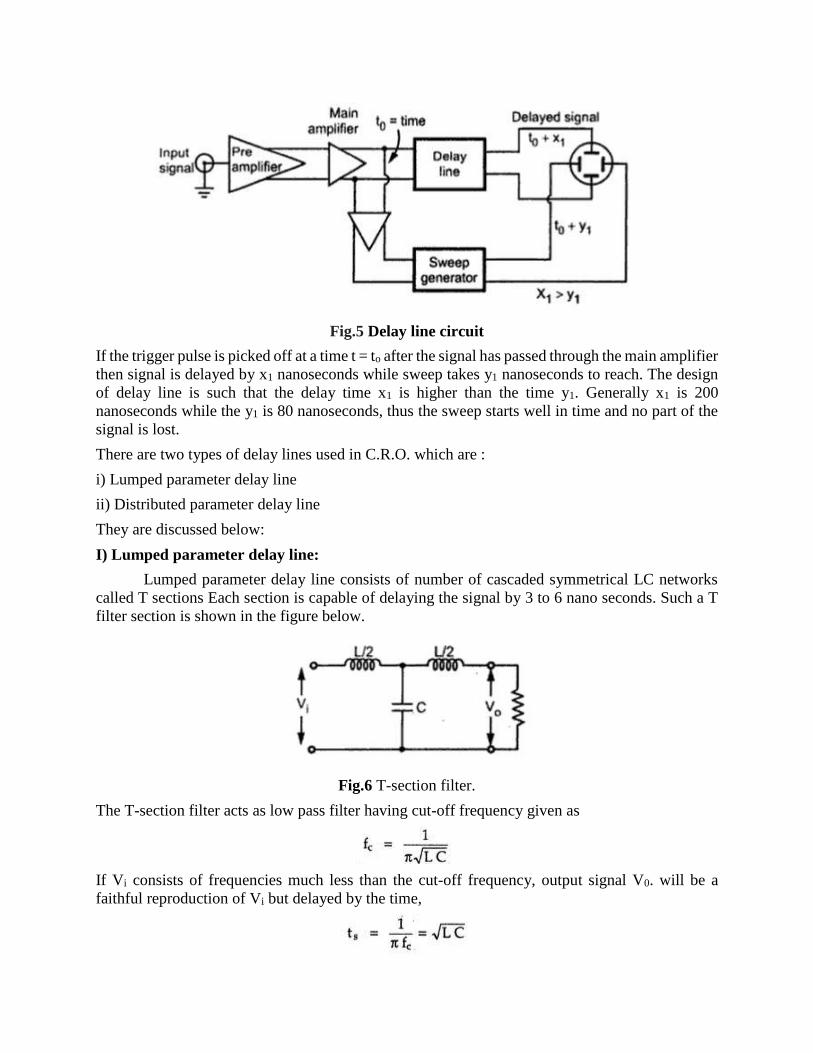
Fig.5 Delay line circuit

If the trigger pulse is picked off at a time t = to after the signal has passed through the main amplifier

then signal is delayed by x1 nanoseconds while sweep takes y1 nanoseconds to reach. The design

of delay line is such that the delay time x1 is higher than the time y1. Generally x1 is 200

nanoseconds while the y1 is 80 nanoseconds, thus the sweep starts well in time and no part of the

signal is lost.

There are two types of delay lines used in C.R.O. which are :

i) Lumped parameter delay line

ii) Distributed parameter delay line

They are discussed below:

I) Lumped parameter delay line:

Lumped parameter delay line consists of number of cascaded symmetrical LC networks

called T sections Each section is capable of delaying the signal by 3 to 6 nano seconds. Such a T

filter section is shown in the figure below.

Fig.6 T-section filter.

The T-section filter acts as low pass filter having cut-off frequency given as

If Vi consists of frequencies much less than the cut-off frequency, output signal V0. will be a

faithful reproduction of Vi but delayed by the time,

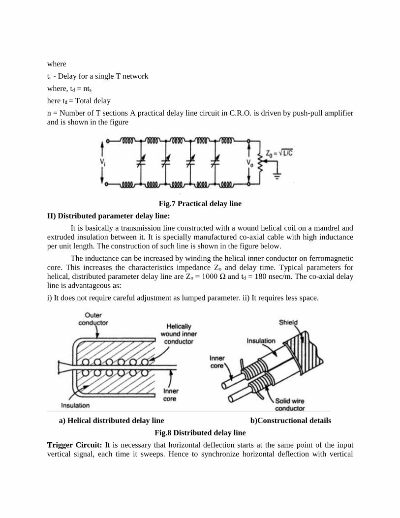
where

ts - Delay for a single T network

where, td = nts

here td = Total delay

n = Number of T sections A practical delay line circuit in C.R.O. is driven by push-pull amplifier

and is shown in the figure

Fig.7 Practical delay line

II) Distributed parameter delay line:

It is basically a transmission line constructed with a wound helical coil on a mandrel and

extruded insulation between it. It is specially manufactured co-axial cable with high inductance

per unit length. The construction of such line is shown in the figure below.

The inductance can be increased by winding the helical inner conductor on ferromagnetic

core. This increases the characteristics impedance Zo and delay time. Typical parameters for

helical, distributed parameter delay line are Zo = 1000 Ω and td = 180 nsec/m. The co-axial delay

line is advantageous as:

i) It does not require careful adjustment as lumped parameter. ii) It requires less space.

a) Helical distributed delay line b)Constructional details

Fig.8 Distributed delay line

Trigger Circuit: It is necessary that horizontal deflection starts at the same point of the input

vertical signal, each time it sweeps. Hence to synchronize horizontal deflection with vertical

deflection a synchronizing or triggering circuit is used. It converts the incoming signal into the

triggering pulses, which are used for the synchronization.

Time Base Generator: The time base generator is used to generate the sawtooth voltage, required

to deflect the beam in the horizontal section. This voltage deflects the spot at a constant time

dependent rate. Thus the x-axis on the screen can be represented as time, which helps to display

and analyse the time varying signals.

Horizontal Amplifier: The sawtooth voltage produced by the time base generator may not be of

sufficient strength. Hence before giving it to the horizontal deflection plates, it is amplified using

the horizontal amplifier.

Power Supply: The power supply block provides the voltages required by CRT to generate and

accelerate an electron beam and voltages required by other circuits of the oscilloscope like

horizontal amplifier, vertical amplifier etc.

The negative High Voltage (HV) supply has following advantages:

i) The accelerating anodes and the deflection plates are close to ground potential. This ground

potential protects the operator from shocks.

ii) The deflection voltages are measured with respect to ground hence blocking or coupling

capacitors are not necessary.

iii) Insulation required between controls and chasis is less.

There are two sections of a power supply block. The High Voltage (HV) section and Low

Voltage (LV) section. The high voltages of the order of 1000V to 1500 V are required by CRT.

Such high negative voltages are used for CRT. The low voltage is required for the heater of the

electron gun, which emits the electrons. This is a positive voltage of the order of few hundred

volts. This voltage is also used for other circuits of C.R.O. This is the discussion of basic block

diagram of a simple C.R.O.

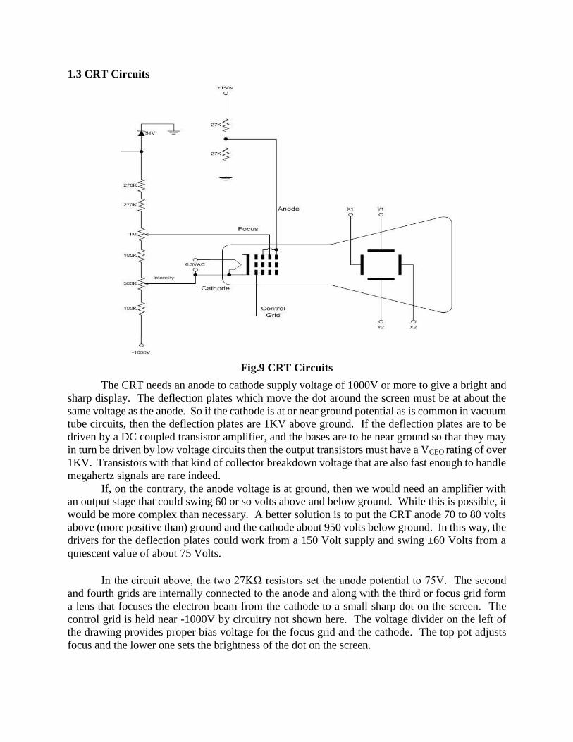
1.3 CRT Circuits

Fig.9 CRT Circuits

The CRT needs an anode to cathode supply voltage of 1000V or more to give a bright and

sharp display. The deflection plates which move the dot around the screen must be at about the

same voltage as the anode. So if the cathode is at or near ground potential as is common in vacuum

tube circuits, then the deflection plates are 1KV above ground. If the deflection plates are to be

driven by a DC coupled transistor amplifier, and the bases are to be near ground so that they may

in turn be driven by low voltage circuits then the output transistors must have a VCEO rating of over

1KV. Transistors with that kind of collector breakdown voltage that are also fast enough to handle

megahertz signals are rare indeed.

If, on the contrary, the anode voltage is at ground, then we would need an amplifier with

an output stage that could swing 60 or so volts above and below ground. While this is possible, it

would be more complex than necessary. A better solution is to put the CRT anode 70 to 80 volts

above (more positive than) ground and the cathode about 950 volts below ground. In this way, the

drivers for the deflection plates could work from a 150 Volt supply and swing ±60 Volts from a

quiescent value of about 75 Volts.

In the circuit above, the two 27KΩ resistors set the anode potential to 75V. The second

and fourth grids are internally connected to the anode and along with the third or focus grid form

a lens that focuses the electron beam from the cathode to a small sharp dot on the screen. The

control grid is held near -1000V by circuitry not shown here. The voltage divider on the left of

the drawing provides proper bias voltage for the focus grid and the cathode. The top pot adjusts

focus and the lower one sets the brightness of the dot on the screen.

Vertical deflection system

The main function of this amplifier is to amplify the weak signal so that the amplified

signal can produce the desired signal. To examine the input signals are penetrated to the vertical

deflection plates through the input attenuator and number of amplifier stages.

The schematic arrangement of the vertical plates, controlling the position of the spot on the

screen is shown in the figure below:

Fig.10 Arrangements of Vertical plates in CRT

The input signals are generally not strong to provide the measurable deflection on the

screen. Hence the vertical amplifier stage is used to amplify the input signals. The amplifier stages

used are generally wide band amplifiers so as to pass faithfully the entire band of frequencies to

be measured. Similarly it contains the attenuator stages as well. The attenuators are used when

very high voltage signals are to be examined, to bring the signals within the proper range of

operation.

The function of vertical deflection system is to provide an amplified signal of the proper

level to drive the vertical deflection plates without introducing any appreciable distortion into the

system. The input sensitivity of many CROs is of the order of a few milli-volts per division and

the voltage required for deflecting the electron beam varies from approximately 100 V (peak to

peak) to 500 V depending on the accelerating voltage and the construction of the tube. Thus the

vertical amplifier is required to provide this desired gain from milli-volt input to several hundred

volt (peak to peak) output. Also the vertical amplifier should not distort the input waveform and

should have good response for entire band of frequencies to be measured. The deflection plates of

CRO act as plates of a capacitor and when the input signal frequency exceeds over 1 MHz, the

current required for charging and discharging of the capacitor formed by the deflection plates

increases. So the vertical amplifier should be capable of supplying current enough to charge and

discharge the deflection plate capacitor.

As we know that electrical signal is delayed by a certain amount of time when transmitted

through an electronic circuitry. In CRO, output signal voltage of the vertical amplifier is fed to the

vertical plates of CRT and some of its portion is used for triggering the time base generator circuit,

whose output is supplied to the horizontal deflection plates through horizontal amplifier. The

whole process, which includes generating and shaping of a trigger pulse and starting of a time-

base generator and then its amplification, takes time of the order of 100 ns or so. So the input signal

of the vertical deflection plates of a CRT is to be delayed by at least the same or little more amount

of time to allow the operator to see the leading edge of the signal waveform under study on the

screen.

The block diagram of a vertical amplifier is shown in the figure below.

Fig.11 Vertical amplifier

It consists of several stages with overall fixed sensitivity. The amplifier can be designed

for stability and required bandwidth very easily due to the fixed gain. The input stage consists of

an attenuator followed by FET source follower. It has very high input impedance required to isolate

the amplifier from the attenuator. It is followed by BJT emitter follower to match the output

impedance of FET output with input of phase inverter. The phase inverter provides two anti-phase

output signals which are required to operate the push pull output amplifier.

The push pull operation has advantages like better hum voltage cancellation, even

harmonic suppression especially large and harmonic, greater power output per tube and reduced

number of defocusing and nonlinear effects.

Triggered sweep

Fig.12 Triggered sweep and its output waveform

The continuous sweep is of limited use in displaying periodic signals of constant frequency

and amplitude. When attempting to display voice or music signals, the pattern falls in and out of

sync as the frequency and amplitude of the music varies resulting in an unstable display.

A triggered sweep can display such signals, and those of short duration, e.g. narrow pulses.

In triggered mode, the input signal is used to generate substantial pulses that trigger the sweep.

Thus ensuring that the sweep is always in step with the signal that drives it.

As shown in figure above, resistance R3 and R4 form a voltage divider such that the voltage

VD at the cathode of the diode is below the peak voltage VP for UJT conduction. When the circuit

is switched on, the UJT is in the non-conducting stage, and CT charges exponentially through RT

towards VBB until the diode becomes forward biased and conducts, the capacitor voltage never

reaches the peak voltage required for UJT conduction but is clamped at VD. If now a -ve pulse of

sufficient amplitude is applied to the base and the peak voltage VP, is momentarily lowered, the

UJT fires. As a result, capacitor CT, discharges rapidly through the UJT until the maintaining

voltage of the UJT is reached; at this point the UJT switches off and capacitor CT charges towards

VBB, until it is clamped again at VD. Above figure shows the output waveform.

1.4 CRO SPECIFICATIONS

Oscilloscopes are a very common form of test equipment - possibly the most important

type of test equipment. As a result it is often necessary to be able to choose one either from the

test equipment store or as a rental or when buying an oscilloscope. When selecting an oscilloscope,

there are many different specifications and parameters to consider, each one related to the

performance. When selecting an oscilloscope, what are the most important specifications and

parameters and which ones will affect the performance of the scope in the particular application.

1) Types of oscilloscope: One of the major specifications associated with buying an oscilloscope

is the actual type of oscilloscope that is required. Some types of scope will be able to perform other

measurements better than others; some use current technology whereas others are older; and there

may be cost implications as well. Analogue, analogue storage, digital, digital storage, digital

sampling, USB scopes and many more types are available.

2) Oscilloscope bandwidth specification: One important oscilloscope specification is related to

the frequency or speed of the waveforms that can be measured. This is determined by the

bandwidth of the oscilloscope and it is found that the capability of the oscilloscope to accurately

display the waveform falls off with increasing frequency. The oscilloscope specification for

bandwidth will typically be quoted in the format: Bandwidth = -3dB at 1500 MHz.

3) Vertical DC gain accuracy: It is important when measuring the amplitude of signals, to know

the accuracy of the measurement that is being made. As oscilloscopes are not intended to be used

instead of digital multimeters, it is not anticipated that the voltage elements of the oscilloscope

specification will be as accurate.

4)Vertical channel Resolution: Digital oscilloscopes need to convert the incoming analogue

signal into a digital signal. The vertical channel resolution determines the "granularity" of the

signal. Most digital oscilloscopes have 8-bit resolution.

5) Rise Time Specification: Another important oscilloscope specification which needs to be

accommodated is the rise time of the oscilloscope. This is a particularly important specification

for any digital circuits where the edges on square waves and pulses are often of great importance.

The oscilloscope must have a sufficiently fast rise time to capture the rapid transitions accurately,

otherwise important information may not be displayed and the results could be misleading. The

rise time of the oscilloscope is defined as the time it takes for the image to rise from 10% to 90%

of the final value.

6) Oscilloscope sample rate: the sample rate oscilloscope specification is becoming a more

widespread and important specification. The sample rate is specified in samples per second (S/s).

The faster the oscilloscope samples the waveform, the greater the resolution of the detail on the

waveform and with greater sample rates the less the likelihood that any critical information will

be lost.

Oscilloscope sample rate = 2.5 x Highest frequency

7) Memory Depth: This is the memory for storing signals. The greater the memory depth the

more signal it is possible to capture at the highest sample rate.

1.5 CRO Controls

The various front panel controls of a simple C.R.O. are described in this section. These are divided

into four groups,

1. Basic controls

2. Vertical section

3. Horizontal section

4. Z-axis Intensity control

1.Basic Controls :

1. ON-OFF : The on-off switch turns on or off the C.R.O.

2. Intensity : This controls the intensity or brightness of the light produced by beam spot. It actually

controls the number of electrons per second that are bombarding the screen which determines the

brightness of the spot.

3. Focus : This controls the sharpness of the spot. A sharper spot is always preferred. Focusing or

the spot is obtained by varying the voltage applied to the focusing anodes of the cathode ray tube.

4. Astigmatism : This is another focus control. With the help of focus control and astigmatism

control, a very sharp spot can be obtained both in the centre and also at the edges of the screen.

With the astigmatism control the voltage to accelerating anodes is varied.

5. Scale Illumination : Most C.R.O. s have some sort of plastic screen in front of the cathode ray

tube. This screen has a grid engraved on it, giving it an appearance similar to that of graph paper.

This is called graticule. This scale facilitates the measurement on the oscilloscope. The scale

illumination control, illuminates the scale and hence the lines on the scale can be seen very easily.

2.Vertical Section: Most oscilloscopes have two vertical inputs. These are usually called inputs 1

and 2 or A and B. Two input signals can be applied to these two inputs and thereby both the signals

can be observed on the screen simultaneously. This is very useful for comparing two signals. The

following controls serve for each vertical input.

a) volts/division:

This control sets the vertical scale; that is, it determines how much the spot will be deflected

by an input signals applied to vertical input terminals. The usual units are either volts per

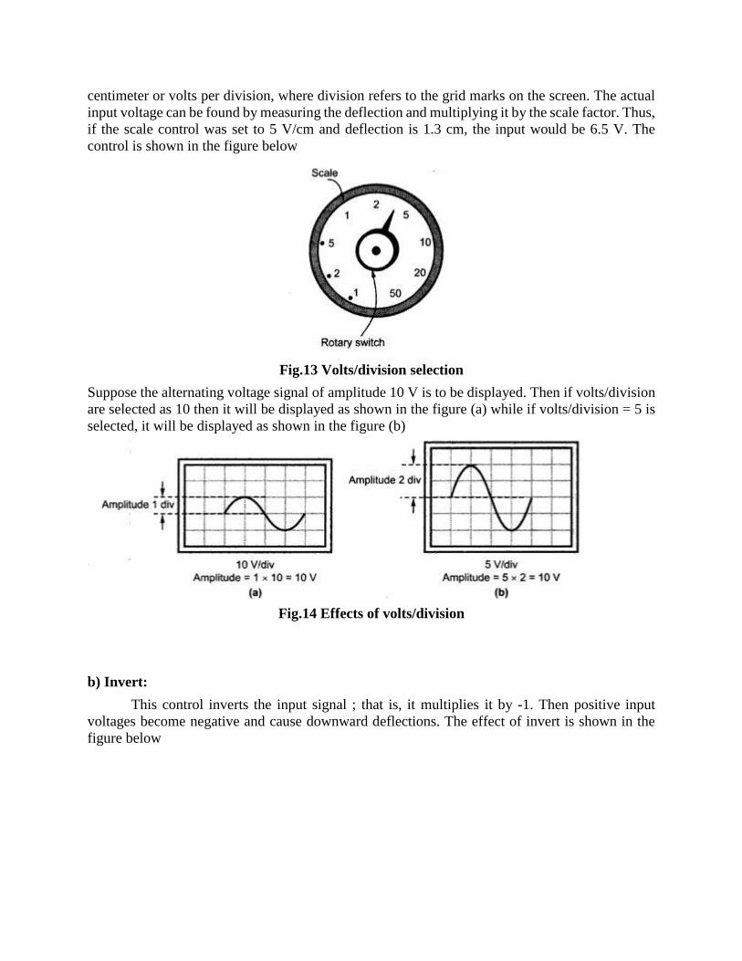
centimeter or volts per division, where division refers to the grid marks on the screen. The actual

input voltage can be found by measuring the deflection and multiplying it by the scale factor. Thus,

if the scale control was set to 5 V/cm and deflection is 1.3 cm, the input would be 6.5 V. The

control is shown in the figure below

Fig.13 Volts/division selection

Suppose the alternating voltage signal of amplitude 10 V is to be displayed. Then if volts/division

are selected as 10 then it will be displayed as shown in the figure (a) while if volts/division = 5 is

selected, it will be displayed as shown in the figure (b)

Fig.14 Effects of volts/division

b) Invert:

This control inverts the input signal ; that is, it multiplies it by -1. Then positive input

voltages become negative and cause downward deflections. The effect of invert is shown in the

figure below

Fig.15 The effect of Invert

c) Position :

With the help of this control, the pattern obtained on the screen can be shifted, as a whole, vertically

upwards or downwards. This is achieved by adding a d.c. offset voltage to the input signal.

d) X 10 (Multiplied by 10):

This control makes the gain of the vertical amplifier 10 times as great as normal, it changes the

scale factor by factor of 10. Thus if the X 10 switch is turned 'ON' and the scope is set on 0.05

V/cm, if the actual scale factor is 0.005 V/cm or 5 mV/cm.

e) Vertical Coupling :

This switch controls the coupling to the vertical amplifier. The usual choices are A.C., D.C., or

ground. The meaning of these various positions are as follows:

i. A.C. : The vertical amplifier is a.c. coupled to the input. Thus the d.c. component of the input is

blocked, and only the a.c. components of the input signal deflect the beam vertically. This allows

to observe small a.c. signals or large d.c. background.

ii. D.C. : The vertical amplifier has d.c. coupling throughout, so that the deflection corresponds to

both the a.c. and the d.c. components of the input.

iii. GROUND : The input to the amplifier is grounded. There will be no vertical deflection. If no

voltage is applied to horizontal plates, the spot will be at the position corresponding to ground. It

is useful for measuring voltage with respect to ground.

f) Vertical Mode Control: The control serves for the vertical section of the scope as a whole.

Assume that two input signals are simultaneously applied to the two vertical inputs of the scope.

Then this switch determines what is displayed on the screen. Thus usual choices are :

1 only, 2 only, 1+2;1-2, Alternate, and Chop. The meaning of each of these is described briefly

below:

i) 1 only : Only the signal at input 1 is displayed.

ii) 2 only : Only the signal at input 2 is displayed.

iii) 1 + 2 : Sum : The sum of the inputs 1 and 2 is displayed.

iv) 1-2 : Sum : Difference : The difference between input 1 and input 2 is displayed.

v) Alternate : Input 1 is displayed first, then input 2 is displayed, then input 1again and so on. By

using the vertical position control, the two traces can be separated vertically, and thus, relations

between the two signals can be studied.

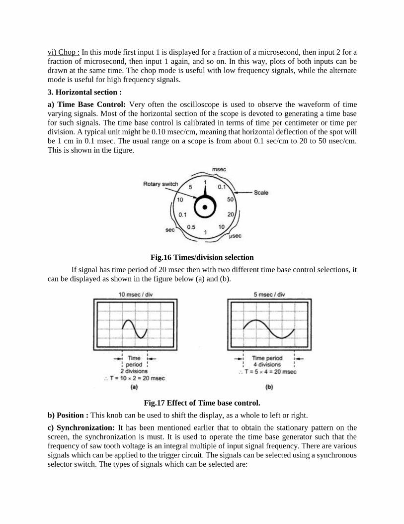
vi) Chop : In this mode first input 1 is displayed for a fraction of a microsecond, then input 2 for a

fraction of microsecond, then input 1 again, and so on. In this way, plots of both inputs can be

drawn at the same time. The chop mode is useful with low frequency signals, while the alternate

mode is useful for high frequency signals.

3. Horizontal section :

a) Time Base Control: Very often the oscilloscope is used to observe the waveform of time

varying signals. Most of the horizontal section of the scope is devoted to generating a time base

for such signals. The time base control is calibrated in terms of time per centimeter or time per

division. A typical unit might be 0.10 msec/cm, meaning that horizontal deflection of the spot will

be 1 cm in 0.1 msec. The usual range on a scope is from about 0.1 sec/cm to 20 to 50 nsec/cm.

This is shown in the figure.

Fig.16 Times/division selection

If signal has time period of 20 msec then with two different time base control selections, it

can be displayed as shown in the figure below (a) and (b).

Fig.17 Effect of Time base control.

b) Position : This knob can be used to shift the display, as a whole to left or right.

c) Synchronization: It has been mentioned earlier that to obtain the stationary pattern on the

screen, the synchronization is must. It is used to operate the time base generator such that the

frequency of saw tooth voltage is an integral multiple of input signal frequency. There are various

signals which can be applied to the trigger circuit. The signals can be selected using a synchronous

selector switch. The types of signals which can be selected are:

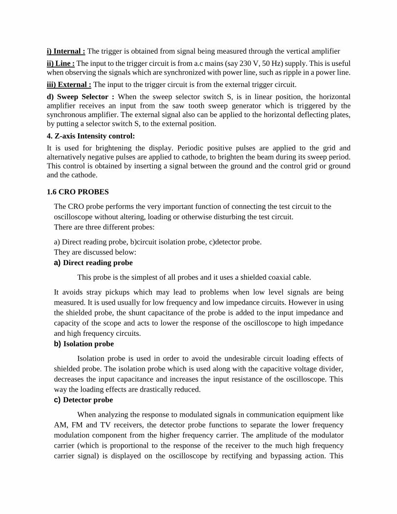
i) Internal : The trigger is obtained from signal being measured through the vertical amplifier

ii) Line : The input to the trigger circuit is from a.c mains (say 230 V, 50 Hz) supply. This is useful

when observing the signals which are synchronized with power line, such as ripple in a power line.

iii) External : The input to the trigger circuit is from the external trigger circuit.

d) Sweep Selector : When the sweep selector switch S, is in linear position, the horizontal

amplifier receives an input from the saw tooth sweep generator which is triggered by the

synchronous amplifier. The external signal also can be applied to the horizontal deflecting plates,

by putting a selector switch S, to the external position.

4. Z-axis Intensity control:

It is used for brightening the display. Periodic positive pulses are applied to the grid and

alternatively negative pulses are applied to cathode, to brighten the beam during its sweep period.

This control is obtained by inserting a signal between the ground and the control grid or ground

and the cathode.

1.6 CRO PROBES

The CRO probe performs the very important function of connecting the test circuit to the

oscilloscope without altering, loading or otherwise disturbing the test circuit.

There are three different probes:

a) Direct reading probe, b)circuit isolation probe, c)detector probe.

They are discussed below:

a) Direct reading probe

This probe is the simplest of all probes and it uses a shielded coaxial cable.

It avoids stray pickups which may lead to problems when low level signals are being

measured. It is used usually for low frequency and low impedance circuits. However in using

the shielded probe, the shunt capacitance of the probe is added to the input impedance and

capacity of the scope and acts to lower the response of the oscilloscope to high impedance

and high frequency circuits.

b) Isolation probe

Isolation probe is used in order to avoid the undesirable circuit loading effects of

shielded probe. The isolation probe which is used along with the capacitive voltage divider,

decreases the input capacitance and increases the input resistance of the oscilloscope. This

way the loading effects are drastically reduced.

c) Detector probe

When analyzing the response to modulated signals in communication equipment like

AM, FM and TV receivers, the detector probe functions to separate the lower frequency

modulation component from the higher frequency carrier. The amplitude of the modulator

carrier (which is proportional to the response of the receiver to the much high frequency

carrier signal) is displayed on the oscilloscope by rectifying and bypassing action. This

permits an oscilloscope capable of audio-frequency response to perform signal tracing tests

on communication signals in the range of hundreds of Mhz, a range which is beyond the

capabilities of all oscilloscopes except the highly specialized ones.

Fig .18: A CRO Probe

1.7 MEASUREMENTS ON CRO

The various characteristics of an input signal and the properties of the signal can be

measured using C.R.O. The various parameters which can be measured using C.R.O. are voltage,

current, period, frequency, phase, amplitude, peak to peak value, duty cycle etc. Let us discuss the

amplitude, frequency and phase measurements using C.R.O.

(1) Voltage measurement:

The C.R.O. includes the amplitude measurement facilities such as constant gain amplifiers

and the calibrated shift controls. The waveform can be adjusted on the screen by using shift

controls so that the measurement of divisions corresponding to the amplitude becomes easy.

Generally to reduce the error, peak to peak value of the signal is measured and then its amplitude

and r.m.s. value is calculated.

To measure the amplitude use the following steps:

1. Note down the selection in volts/ division from the front panel, selected for measurement

2. Adjust shift control to adjust signal on screen so that it becomes easy to count number of

divisions corresponding to peak to peak value of the signal.

3. Note down peak to peak value in terms of the number of divisions on screen.

4. Use the following relation to obtain peak to peak value in volts.

5.The amplitude can then be calculated as :

while the rms value of sinusoidal wave can be given as:

(2) Current measurement:

Fig.19 Arrangement for current measurement

The CRO is basically voltage indicating device. Hence to measure the current, the current

is passed through a known standard resistance. The voltage across resistance is displayed on CRO

and is measured. This measured voltage divided by the known resistance gives the value of the

unknown current. The arrangement is shown in the figure above. Current is obtained using

formula,

(3) Period & Frequency measurement:

In such measurement, the waveform is displayed on the screen such that one complete

cycle is visible on the screen. Thus accuracy increases if a single cycle occupies as much as the

horizontal distance on the screen.

Note the time/ division selected on the front panel. Then the period of the waveform can be

obtained as,

The frequency is the reciprocal of the period. That is given by:

This is the method of frequency measurement without Lissajous pattern.

1.8 MEASUREMENT OF PHASE AND FREQUENCY USING LISSAJOUS PATTERNS:

It is interesting to consider the characteristics of patterns that appear on the screen of a

CRT when sinusoidal voltages are simultaneously applied to horizontal and vertical plates. These

patterns are called 'Lissajous Patterns'. When two sinusoidal voltages of equal frequency which

are in phase with each other are applied to the horizontal and vertical deflection plates, the pattern

appearing on the screen is a straight line as its clear from figure below

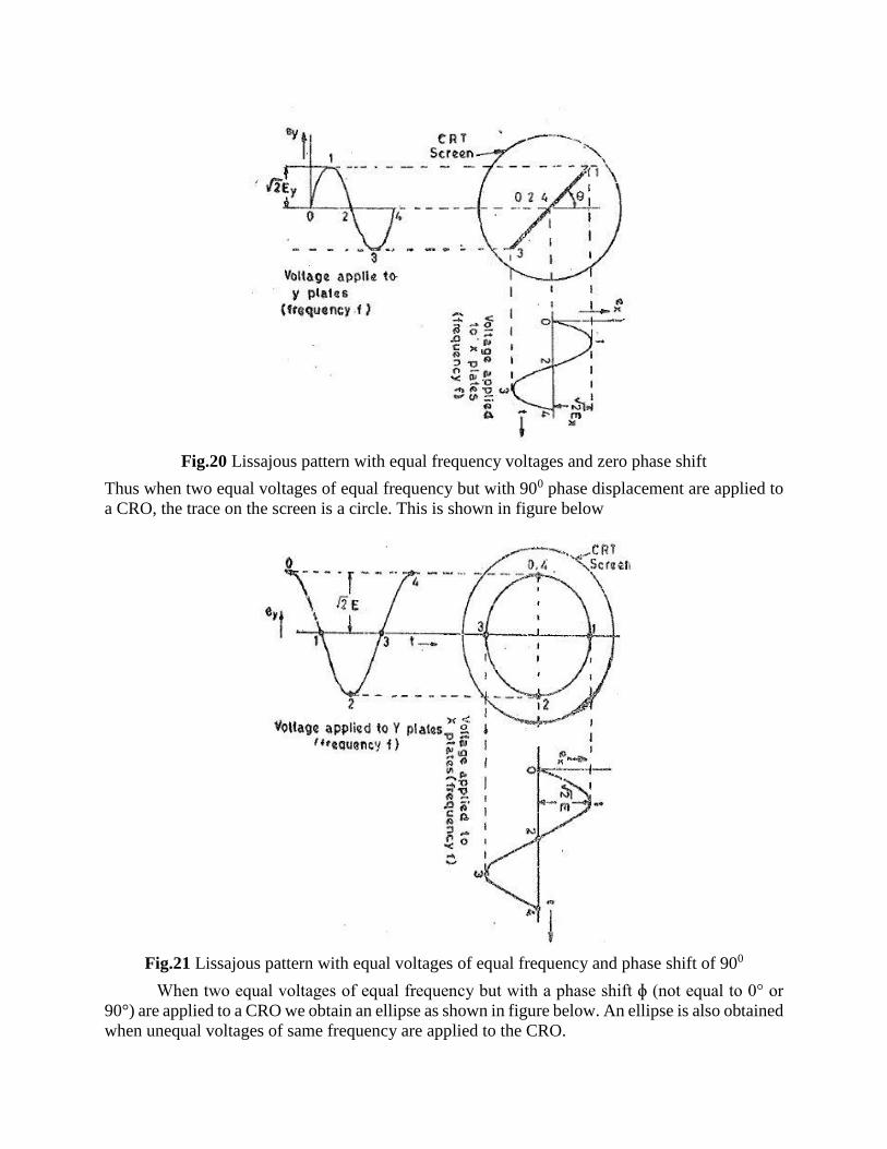
Fig.20 Lissajous pattern with equal frequency voltages and zero phase shift

Thus when two equal voltages of equal frequency but with 900 phase displacement are applied to

a CRO, the trace on the screen is a circle. This is shown in figure below

Fig.21 Lissajous pattern with equal voltages of equal frequency and phase shift of 900

When two equal voltages of equal frequency but with a phase shift ɸ (not equal to 0° or

90°) are applied to a CRO we obtain an ellipse as shown in figure below. An ellipse is also obtained

when unequal voltages of same frequency are applied to the CRO.

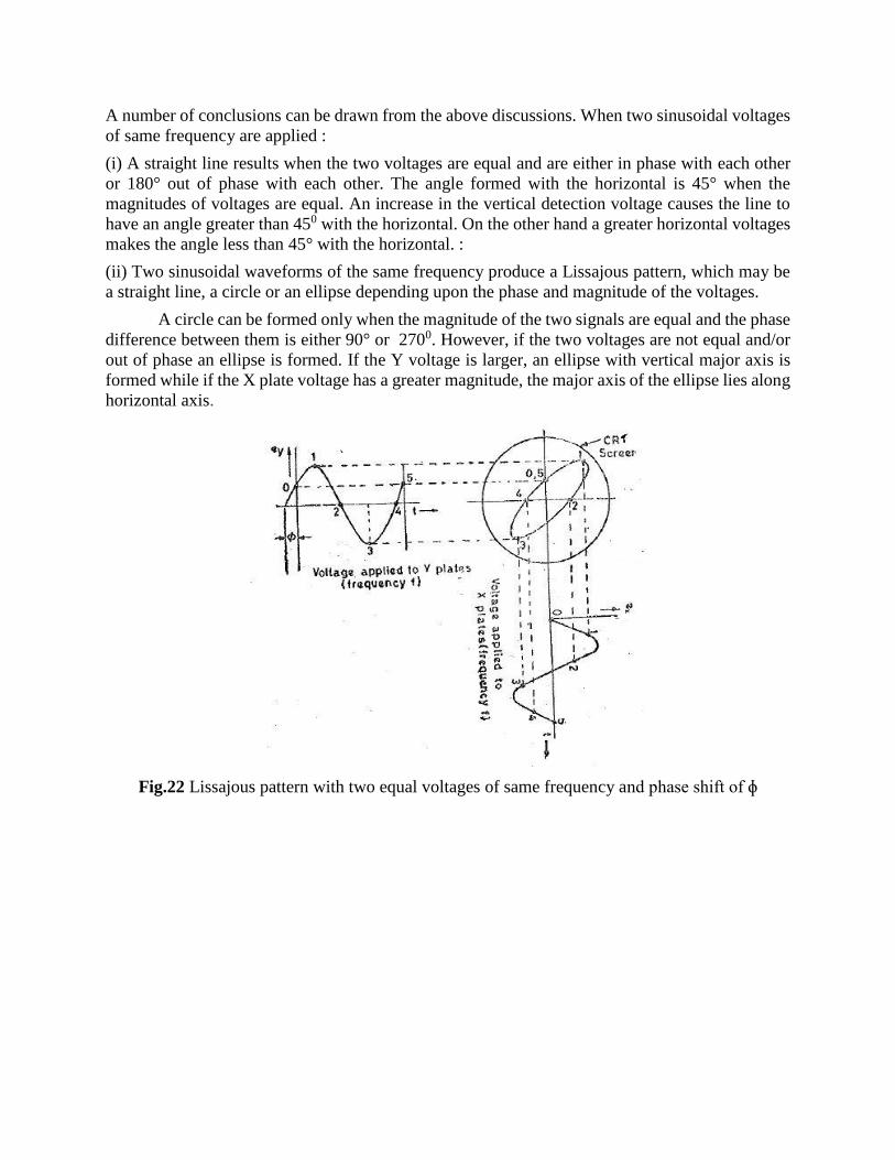
A number of conclusions can be drawn from the above discussions. When two sinusoidal voltages

of same frequency are applied :

(i) A straight line results when the two voltages are equal and are either in phase with each other

or 180° out of phase with each other. The angle formed with the horizontal is 45° when the

magnitudes of voltages are equal. An increase in the vertical detection voltage causes the line to

have an angle greater than 450 with the horizontal. On the other hand a greater horizontal voltages

makes the angle less than 45° with the horizontal. :

(ii) Two sinusoidal waveforms of the same frequency produce a Lissajous pattern, which may be

a straight line, a circle or an ellipse depending upon the phase and magnitude of the voltages.

A circle can be formed only when the magnitude of the two signals are equal and the phase

difference between them is either 90° or 2700. However, if the two voltages are not equal and/or

out of phase an ellipse is formed. If the Y voltage is larger, an ellipse with vertical major axis is

formed while if the X plate voltage has a greater magnitude, the major axis of the ellipse lies along

horizontal axis.

Fig.22 Lissajous pattern with two equal voltages of same frequency and phase shift of ɸ

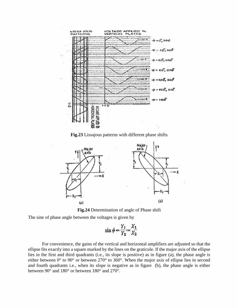
Fig.23 Lissajous patterns with different phase shifts

Fig.24 Determination of angle of Phase shift

The sine of phase angle between the voltages is given by

For convenience, the gains of the vertical and horizontal amplifiers are adjusted so that the

ellipse fits exactly into a square marked by the lines on the graticule. If the major axis of the ellipse

lies in the first and third quadrants (i.e., its slope is positive) as in figure (a), the phase angle is

either between 0° to 90° or between 270° to 360°. When the major axis of ellipse lies in second

and fourth quadrants i.e., when its slope is negative as in figure (b), the phase angle is either

between 90° and 180° or between 180° and 270°.

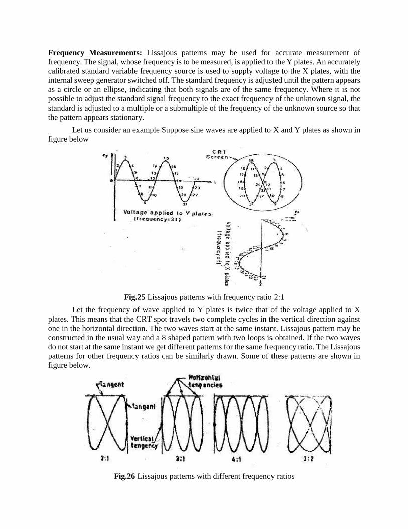
Frequency Measurements: Lissajous patterns may be used for accurate measurement of

frequency. The signal, whose frequency is to be measured, is applied to the Y plates. An accurately

calibrated standard variable frequency source is used to supply voltage to the X plates, with the

internal sweep generator switched off. The standard frequency is adjusted until the pattern appears

as a circle or an ellipse, indicating that both signals are of the same frequency. Where it is not

possible to adjust the standard signal frequency to the exact frequency of the unknown signal, the

standard is adjusted to a multiple or a submultiple of the frequency of the unknown source so that

the pattern appears stationary.

Let us consider an example Suppose sine waves are applied to X and Y plates as shown in

figure below

Fig.25 Lissajous patterns with frequency ratio 2:1

Let the frequency of wave applied to Y plates is twice that of the voltage applied to X

plates. This means that the CRT spot travels two complete cycles in the vertical direction against

one in the horizontal direction. The two waves start at the same instant. Lissajous pattern may be

constructed in the usual way and a 8 shaped pattern with two loops is obtained. If the two waves

do not start at the same instant we get different patterns for the same frequency ratio. The Lissajous

patterns for other frequency ratios can be similarly drawn. Some of these patterns are shown in

figure below.

Fig.26 Lissajous patterns with different frequency ratios

It can be shown that for all the above cases, the ratios of the two frequencies is :

where, fV = frequency of signal applied to Y-plates

fX = frequency of signal applied to X-plates

1.9 TYPES OF OSCILLOSCOPES

There are a number of oscilloscopes which are used for special applications.

Some of the oscilloscopes are described below:

a) Multiple beam oscilloscopes

In many cases it becomes necessary to compare one signal with that of the other. In

such cases Multiple beam oscilloscopes are used. They enclose in a single tube several beam

producing systems each with its vertical pair of plates, but mostly with a common time-base.

Each Y-channel has its own amplifier. The synchronization or triggering is done from the

input of a desired Y-channel or from an external input voltage.

Double beam oscilloscopes use two electron guns within the same cathode ray tube. the

electron beam of the two channels are completely independent of each other. The same effect

may be produced by a single electron gun, the output from it being split into two.

b) Multiple Trace Oscilloscopes

This oscilloscope uses single electron guns and produces multiple traces by switching

the Y-deflection plates from one input signal to another (this means that the Y- channel is time

shared by many signals). The eyes interpret this is a continuous simultaneous display of the

input signals although it is a sampled display. This method reduces the cost of manufacturing

multi-channel oscilloscopes.

c) Sampling oscilloscopes

The oscilloscopes presently can be used for continuous display for frequencies in the

50-300 Mhz range depending upon the design of the oscilloscopes. The display may have upto

1000 dots of luminescence. The vertical deflection for each dot is obtained from progressively

later points in each successive cycle of input waveform as shown below:

27

Fig.27 Principle of Sampling Oscilloscopes.

The horizontal deflection of the electron beam is obtained by applying staircase

waveform to X-deflection plates.The sampling oscilloscope is able to respond and store

rapid bits of information and present them in a continuous display. The sampling

techniques immediately the input signals into lower frequency domain, where

conventional low frequency circuitry is then capable of producing a highly effective

display.This type of oscilloscopes can be used beyond 50Mhz into the UHF range around

500Mhz and beyond upto 10Ghz. It should be noted that the sampling techniques cannot

be used the display of transient waveforms.

Sampling Oscilloscope

An ordinary oscilloscope has a Bandwidth of 10 MHz. The high frequency (HF) performance

can be improved by means of sampling the input waveform and reconstructing its shape from

the sample, i.e. the signal to be observed is sampled and after a few cycles the sampling point

is advanced and another sample is taken. The shape of the waveform is reconstructed by joining

the sample levels together. The sampling frequency may be as low as 1/10th of the input signal

frequency (if the input signal frequency is 100 MHz, the bandwidth of the CRO vertical

amplifier can be as low as 10 MHz). As many as 1000 samples are used to reconstruct the

original waveform. Figure below shows a block diagram of a sampling oscilloscope.

Fig.28 Block diagram of Digital Sampling Oscilloscope

28

The input waveform is applied to the sampling gate. The input waveform is sampled

whenever a sampling pulse opens the sampling gate. The sampling must be synchronized with

the input signal frequency. The signal is delayed in the vertical amplifier, allowing the

horizontal sweep to be initiated by the input signal. The corresponding waveforms are also

shown in below figure

Fig.31 Various waveforms at each block of a sampling oscilloscope.

At the beginning of each sampling cycle, the trigger pulse activates an oscillator and a

linear ramp voltage is generated. This ramp voltage is applied to a voltage comparator which

compares the ramp voltage to a staircase generator, When the two voltages are equal in

amplitude, the staircase advances one step and a sampling pulse is generated, which opens the

sampling gate for a sample of input voltage.

The resolution of the final image depends upon the size of the steps of the staircase

generator. The smaller the size of the steps the larger the number of samples and higher the

resolution of the image.

d) Scanning Oscilloscopes

These oscilloscopes use television tubes. The data to be measured are applied

through intensity modulation on the standard screen. Several phenomena can be observed

simultaneously on a single screen by using this technique. As a result of large number of

factors influencing the quality of recording, experience with the particular camera CRO

combination is usually the best guide.

e) Storage type Oscilloscopes

They are rapidly becoming one of the most useful tools in the presentation of very

slowly swept signals and finds many application in mechanical and biomedical

fields.

Usually in conventional CRTs, the persistence of phosphor ranges from

microseconds to seconds. In applications where the persistence of the screen is

smaller than the rate at which the signal sweeps across the screen, the start of

screen will have disappeared before the end of the display is written.

In storage oscilloscopes, the persistence times are much greater than a few

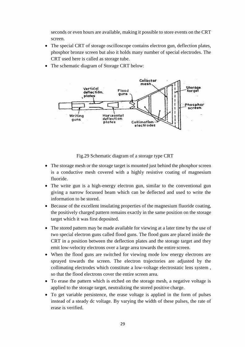
29

seconds or even hours are available, making it possible to store events on the CRT

screen.

The special CRT of storage oscilloscope contains electron gun, deflection plates,

phosphor bronze screen but also it holds many number of special electrodes. The

CRT used here is called as storage tube.

The schematic diagram of Storage CRT below:

Fig.29 Schematic diagram of a storage type CRT

The storage mesh or the storage target is mounted just behind the phosphor screen

is a conductive mesh covered with a highly resistive coating of magnesium

fluoride.

The write gun is a high-energy electron gun, similar to the conventional gun

giving a narrow focussed beam which can be deflected and used to write the

information to be stored.

Because of the excellent insulating properties of the magnesium fluoride coating,

the positively charged pattern remains exactly in the same position on the storage

target which it was first deposited.

The stored pattern may be made available for viewing at a later time by the use of

two special electron guns called flood guns. The flood guns are placed inside the

CRT in a position between the deflection plates and the storage target and they

emit low-velocity electrons over a large area towards the entire screen.

When the flood guns are switched for viewing mode low energy electrons are

sprayed towards the screen. The electron trajectories are adjusted by the

collimating electrodes which constitute a low-voltage electrostatic lens system ,

so that the flood electrons cover the entire screen area.

To erase the pattern which is etched on the storage mesh, a negative voltage is

applied to the storage target, neutralizing the stored positive charge.

To get variable persistence, the erase voltage is applied in the form of pulses

instead of a steady dc voltage. By varying the width of these pulses, the rate of

erase is verified.

30

f) Impulse waveform oscilloscopes

These oscilloscopes are used for the investigation of transient non-period

phenomena which occur at high voltages. These oscilloscopes use special types of CRT

wherein the plates are mounted on the sides. The voltage to be measured is applied to these

plates either directly or through capacitive potential dividers. Simultaneously, an impulse

is suddenly applied to the cathode voltage. A very bright display is obtained on account of

the high voltage and the high beam current which exist for a very short duration. Therefore,

photographic records of the display can be obtained even at very high speeds of upto

50x106 m/s.

1.9 STORAGE CRO, DIGITAL STORAGE OSCILLOSCOPE

The storage type CRO is rapidly becoming one of the most useful tools in the

presentation of very slowly swept signals and finds many applications in the mechanical and

biomedical fields. In the conventional CRT the persistence of the phosphor ranges from micro

seconds to perhaps seconds. In applications where the persistence of the screen is smaller than

the rate at which the signal sweeps across the screen, the start of the display will have

disappeared before the end of the display is written.

With the variable-persistence or storage CRO, the slowly swept trace can be kept on

display continuously by adjusting the persistence of the CRT screen to match the sweep time.

Persistence times much greater than a few seconds or even hours, are available, making it

possible to store events on a CRT screen. The storage CRO uses a special CRT, called the

storage tube. This special CRT contains all the elements of a conventional CRT, such as the

electron gun, the deflection plates, and a phosphor screen, but in addition holds a number of

special electrodes A schematic representation of one type storage tube is given in figure below.

The storage mesh or storage target, mounted just behind the phosphor screen, is a

conductive mesh covered with a highly resistive coating of magnesium fluoride. The write gun

is a high-energy electron gun, similar to the conventional gun, giving a narrow focussed beam

which can be deflected and used to write the information to be stored. The write gun etches a

positively charged pattern on the storage target by knocking off secondary-emission electrons.

Because of the excellent insulating properties of the magnesium fluoride coating, this positively

charged pattern remains exactly in the same position on the storage target where it was first

deposited. The electron beam, which is deflected in the conventional manner both in the

horizontal and the vertical directions, therefore traces out the waveform pattern on the storage

target.

Fig.30 Schematic diagram of Storage type CRT

31

The stored pattern may be made available for viewing at a later time by the use of two

special electron guns, called flood guns. The flood guns are placed inside the CRT in a position

between the deflection plates and the storage target and they emit low-velocity electrons over

a large area towards the entire screen. When the flood guns are switched on (the viewing mode),

low energy electrons are sprayed towards the screen. The electron trajectories are adjusted by

the collimation electrodes which constitute a low voltage electrostatic lens system, so that the

flood-electrons cover the entire screen area. Most of the flood electrons are collected by the

collector mesh and therefore never reach the phosphor screen. In the area near the stored

positive charge on the storage target, the positive field pulls some of the flood-electrons through

the storage mesh and these electrons continue to hit the phosphor. The CRT display therefore

will be an exact copy of the pattern which was initially stored on the target and the display will

be visible as long as the flood guns continue emission of low-energy electrons. To erase the

pattern which is etched on the storage mesh, a negative voltage is applied to the storage target,

neutralizing the stored positive charge.

To obtain variable persistence, the erase voltage is applied in the form of pulses instead

of a steady d.c. voltage. By varying the width of these pulses the rate of erasing is varied. The

variable-persistence control on the front panel of the scope is then the width control of the

erase-pulse generator.

2.INDUSTRIAL APPLICATIONS OF CRO

Because the oscilloscope is an extremely flexible and versatile instrument, it can

be used to measure a number of parameters associated with DC and AC signals. Using a

single channel oscilloscope, it is capable of making measurements of voltage current, time,

frequency and rise/fall time. If a dual trace oscilloscope is used the phase shift between

two synchronous signals can be measured.

Other major applications of CRO are listed below:

In Radio Work

1. To trace and measure a signal throughout the RF, IF and AF channels of radio and

television receivers.

2. It provides the only effective way of adjusting FM receivers, broadband high-

frequency RF amplifiers and automatic frequency control circuits;

3. to test AF circuits for different types of distortions and other spurious oscillations;

4. To give visual display of wave-shapes such as sine waves, square waves and their

many different combinations;

5. To trace transistor curves

6. To visually show the composite synchronized TV signal

7. To display the response of tuned circuits etc.

Scientific and Engineering applications:

1. Measurement of ac/dc voltages,

2. Finding B/H curves for hysteresis loop,

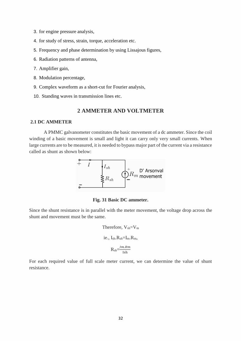
32

3. for engine pressure analysis,

4. for study of stress, strain, torque, acceleration etc.

5. Frequency and phase determination by using Lissajous figures,

6. Radiation patterns of antenna,

7. Amplifier gain,

8. Modulation percentage,

9. Complex waveform as a short-cut for Fourier analysis,

10. Standing waves in transmission lines etc.

2 AMMETER AND VOLTMETER

2.1 DC AMMETER

A PMMC galvanometer constitutes the basic movement of a dc ammeter. Since the coil

winding of a basic movement is small and light it can carry only very small currents. When

large currents are to be measured, it is needed to bypass major part of the current via a resistance

called as shunt as shown below:

Fig. 31 Basic DC ammeter.

Since the shunt resistance is in parallel with the meter movement, the voltage drop across the

shunt and movement must be the same.

Therefore, Vsh=Vm

ie., Ish.Rsh=Im.Rm,

Rsh=𝐼𝑚.𝑅𝑚

Ish

For each required value of full scale meter current, we can determine the value of shunt

resistance.

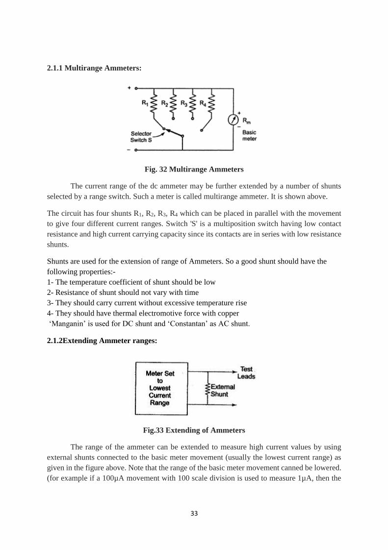
33

2.1.1 Multirange Ammeters:

Fig. 32 Multirange Ammeters

The current range of the dc ammeter may be further extended by a number of shunts

selected by a range switch. Such a meter is called multirange ammeter. It is shown above.

The circuit has four shunts R1, R2, R3, R4 which can be placed in parallel with the movement

to give four different current ranges. Switch 'S' is a multiposition switch having low contact

resistance and high current carrying capacity since its contacts are in series with low resistance

shunts.

Shunts are used for the extension of range of Ammeters. So a good shunt should have the

following properties:-

1- The temperature coefficient of shunt should be low

2- Resistance of shunt should not vary with time

3- They should carry current without excessive temperature rise

4- They should have thermal electromotive force with copper

‘Manganin’ is used for DC shunt and ‘Constantan’ as AC shunt.

2.1.2Extending Ammeter ranges:

Fig.33 Extending of Ammeters

The range of the ammeter can be extended to measure high current values by using

external shunts connected to the basic meter movement (usually the lowest current range) as

given in the figure above. Note that the range of the basic meter movement canned be lowered.

(for example if a 100µA movement with 100 scale division is used to measure 1µA, then the

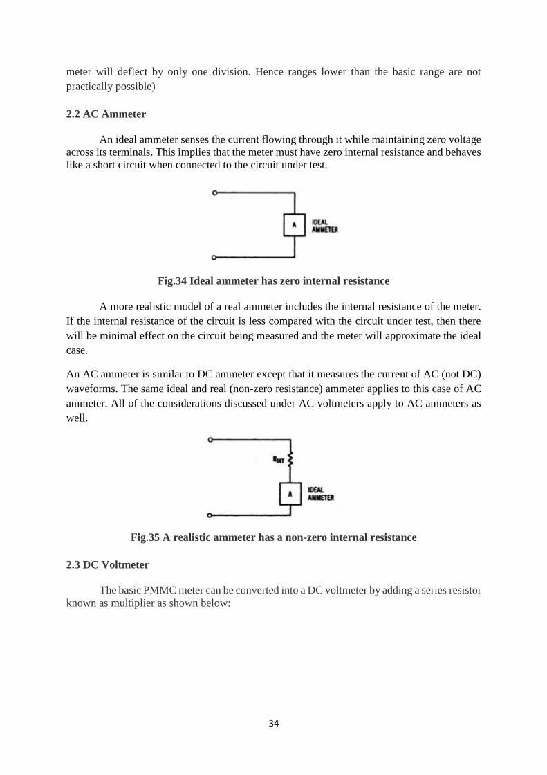
34

meter will deflect by only one division. Hence ranges lower than the basic range are not

practically possible)

2.2 AC Ammeter

An ideal ammeter senses the current flowing through it while maintaining zero voltage

across its terminals. This implies that the meter must have zero internal resistance and behaves

like a short circuit when connected to the circuit under test.

Fig.34 Ideal ammeter has zero internal resistance

A more realistic model of a real ammeter includes the internal resistance of the meter.

If the internal resistance of the circuit is less compared with the circuit under test, then there

will be minimal effect on the circuit being measured and the meter will approximate the ideal

case.

An AC ammeter is similar to DC ammeter except that it measures the current of AC (not DC)

waveforms. The same ideal and real (non-zero resistance) ammeter applies to this case of AC

ammeter. All of the considerations discussed under AC voltmeters apply to AC ammeters as

well.

Fig.35 A realistic ammeter has a non-zero internal resistance

2.3 DC Voltmeter

The basic PMMC meter can be converted into a DC voltmeter by adding a series resistor

known as multiplier as shown below:

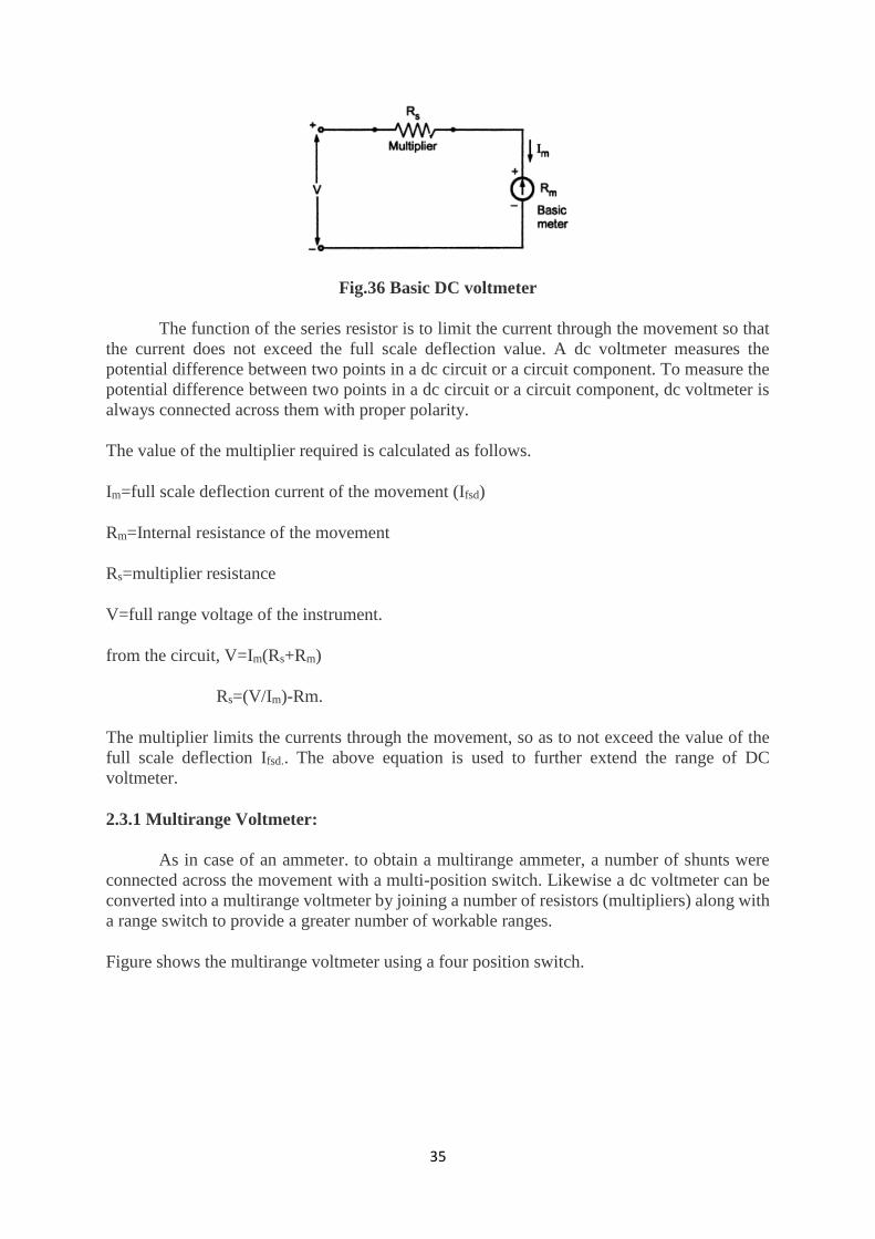
35

Fig.36 Basic DC voltmeter

The function of the series resistor is to limit the current through the movement so that

the current does not exceed the full scale deflection value. A dc voltmeter measures the

potential difference between two points in a dc circuit or a circuit component. To measure the

potential difference between two points in a dc circuit or a circuit component, dc voltmeter is

always connected across them with proper polarity.

The value of the multiplier required is calculated as follows.

Im=full scale deflection current of the movement (Ifsd)

Rm=Internal resistance of the movement

Rs=multiplier resistance

V=full range voltage of the instrument.

from the circuit, V=Im(Rs+Rm)

Rs=(V/Im)-Rm.

The multiplier limits the currents through the movement, so as to not exceed the value of the

full scale deflection Ifsd.. The above equation is used to further extend the range of DC

voltmeter.

2.3.1 Multirange Voltmeter:

As in case of an ammeter. to obtain a multirange ammeter, a number of shunts were

connected across the movement with a multi-position switch. Likewise a dc voltmeter can be

converted into a multirange voltmeter by joining a number of resistors (multipliers) along with

a range switch to provide a greater number of workable ranges.

Figure shows the multirange voltmeter using a four position switch.

36

Fig.37 Multirange Voltmeter

2.3.2 Extending Voltmeter ranges:

The range of a voltmeter can be extended to measure high voltages by using a high

voltage probe or by using an external multiplier resistor as shown below:

Fig.38 Extending Voltmeter ranges.

In most meters the basic movement is used on the lowest current range.

2.4 AC VOLTMETER

In electronic ac voltmeters input signal is firstly rectified and then supplied to the dc

amplifier, as shown in figure. Sometimes signal is firstly amplified by ac amplifier and then

rectified before supplying it to dc meter, as shown in figure.

Fig.39 AC Voltmeters

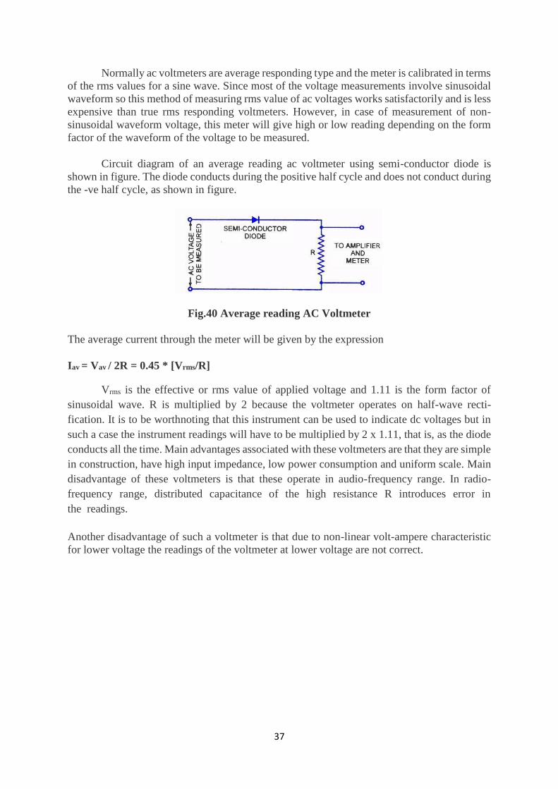
37

Normally ac voltmeters are average responding type and the meter is calibrated in terms

of the rms values for a sine wave. Since most of the voltage measurements involve sinusoidal

waveform so this method of measuring rms value of ac voltages works satisfactorily and is less

expensive than true rms responding voltmeters. However, in case of measurement of non-

sinusoidal waveform voltage, this meter will give high or low reading depending on the form

factor of the waveform of the voltage to be measured.

Circuit diagram of an average reading ac voltmeter using semi-conductor diode is

shown in figure. The diode conducts during the positive half cycle and does not conduct during

the -ve half cycle, as shown in figure.

Fig.40 Average reading AC Voltmeter

The average current through the meter will be given by the expression

Iav = Vav / 2R = 0.45 * [Vrms/R]

Vrms is the effective or rms value of applied voltage and 1.11 is the form factor of

sinusoidal wave. R is multiplied by 2 because the voltmeter operates on half-wave recti-

fication. It is to be worthnoting that this instrument can be used to indicate dc voltages but in

such a case the instrument readings will have to be multiplied by 2 x 1.11, that is, as the diode

conducts all the time. Main advantages associated with these voltmeters are that they are simple

in construction, have high input impedance, low power consumption and uniform scale. Main

disadvantage of these voltmeters is that these operate in audio-frequency range. In radio-

frequency range, distributed capacitance of the high resistance R introduces error in

the readings.

Another disadvantage of such a voltmeter is that due to non-linear volt-ampere characteristic

for lower voltage the readings of the voltmeter at lower voltage are not correct.

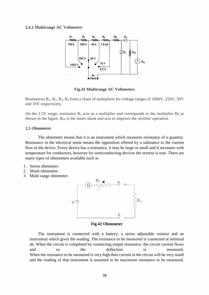
38

2.4.1 Multirange AC Voltmeter:

Fig.41 Multirange AC Voltmeters

Resistances R1, R2, R3, R4 form a chain of multipliers for voltage ranges of 1000V, 250V, 50V

and 10V respectively.

On the 2.5V range, resistance R5 acts as a multiplier and corresponds to the multiplier Rs as

shown in the figure. Rsh is the meter shunt and acts to improve the rectifier operation.

2.5 Ohmmeter

The ohmmeter means that it is an instrument which measures resistance of a quantity.

Resistance in the electrical sense means the opposition offered by a substance to the current

flow in the device. Every device has a resistance, it may be large or small and it increases with

temperature for conductors, however for semiconducting devices the reverse is true. There are

many types of ohmmeters available such as

1. Series ohmmeter.

2. Shunt ohmmeter.

3. Multi range ohmmeter.

Fig.42 Ohmmeter

The instrument is connected with a battery, a series adjustable resistor and an

instrument which gives the reading. The resistance to be measured is connected at terminal

ab. When the circuit is completed by connecting output resistance, the circuit current flows

and so the deflection is measured.

When the resistance to be measured is very high then current in the circuit will be very small

and the reading of that instrument is assumed to be maximum resistance to be measured.

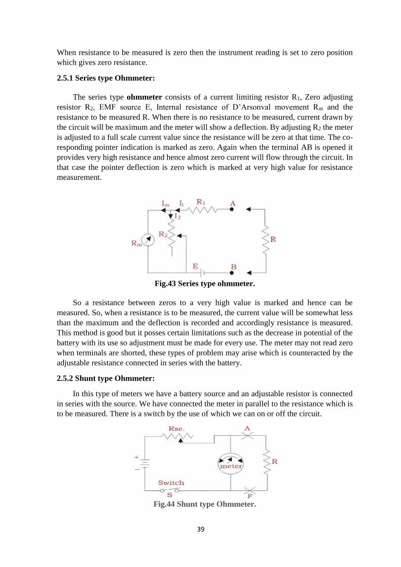
39

When resistance to be measured is zero then the instrument reading is set to zero position

which gives zero resistance.

2.5.1 Series type Ohmmeter:

The series type ohmmeter consists of a current limiting resistor R1, Zero adjusting

resistor R2, EMF source E, Internal resistance of D’Arsonval movement Rm and the

resistance to be measured R. When there is no resistance to be measured, current drawn by

the circuit will be maximum and the meter will show a deflection. By adjusting R2 the meter

is adjusted to a full scale current value since the resistance will be zero at that time. The co-

responding pointer indication is marked as zero. Again when the terminal AB is opened it

provides very high resistance and hence almost zero current will flow through the circuit. In

that case the pointer deflection is zero which is marked at very high value for resistance

measurement.

Fig.43 Series type ohmmeter.

So a resistance between zeros to a very high value is marked and hence can be

measured. So, when a resistance is to be measured, the current value will be somewhat less

than the maximum and the deflection is recorded and accordingly resistance is measured.

This method is good but it posses certain limitations such as the decrease in potential of the

battery with its use so adjustment must be made for every use. The meter may not read zero

when terminals are shorted, these types of problem may arise which is counteracted by the

adjustable resistance connected in series with the battery.

2.5.2 Shunt type Ohmmeter:

In this type of meters we have a battery source and an adjustable resistor is connected

in series with the source. We have connected the meter in parallel to the resistance which is

to be measured. There is a switch by the use of which we can on or off the circuit.

Fig.44 Shunt type Ohmmeter.

40

The switch is opened when it is not in use. When the resistance to be measured is zero,

the terminals A and F are shorted so the current through the meter will be zero. The zero

position of the meter denotes the resistance to be zero. When the resistance connected is very

high, then a small current will flow through the terminal AF and hence full scale current is

allowed to flow through the meter by adjusting the series resistance connected with the

battery. So, full scale deflection measures very high resistance. When the resistance to be

measured is connected between A and F, The pointer shows a deflection by which we can

measure the resistance values. In this case also, the battery problem may arise which can be

counteracted by adjusting the resistance. The meter may have some error due to its repeated

use also.

2.5.3 Multirange Ohmmeter:

This instrument provides the reading up to a very wide range. In this case we have to

select the range switch according to our requirement. An adjuster is provided so that we can

adjust the initial reading to be zero. The resistance to be measured is connected in parallel

to the meter.

Fig. 45 Multirange Ohmmeter.

The meter is adjusted so that it shows full scale deflection when the terminals in which

the resistance connected is full scale range connected through the range switch. When the

resistance is zero or short circuit, there is no current flow through the meter and hence no

deflection. Suppose we have to measure a resistance under 1 ohm, then the range switch is

selected at 1 ohm range at first. Then that resistance is connected in parallel and the

corresponding meter deflection is noted. For 1 ohm resistance it shows full scale deflection but

for the resistance other that 1 ohm it shows a deflection which is less than the full load value

and hence resistance can be measured. This is the most suitable method of all the ohmmeters as

we can get accurate reading in this type of meters. So this meter is most widely used now days.

41

2.3 ELECTRONIC MULTIMETERS

A multimeter is basically a PMMC meter. To measure dc current the meter acts as an

ammeter with a low series resistance. Range changing is accomplished by shunts in such a way

that the current passing through the meter does not exceed the maximum rated value. A

multimeter consists of an ammeter, voltmeter and ohmmeter combined with a function switch

to connect the appropriate circuit to the D'Arsonval movement.

Fig. 46 Diagram of a multimeter

The above figure shows the circuit diagram of a multimeter used as a microammeter, ac

voltmeter, dc voltmeter, dc milliammeter and an ohmmeter.

2.3.1 Microammeter & DC ammeter

Following figure shows the circuit of a multimeter used as a microammeter as well as

its use as a dc ammeter.

Fig. 47 Multimeter as a microammeter and as a dc ammeter.

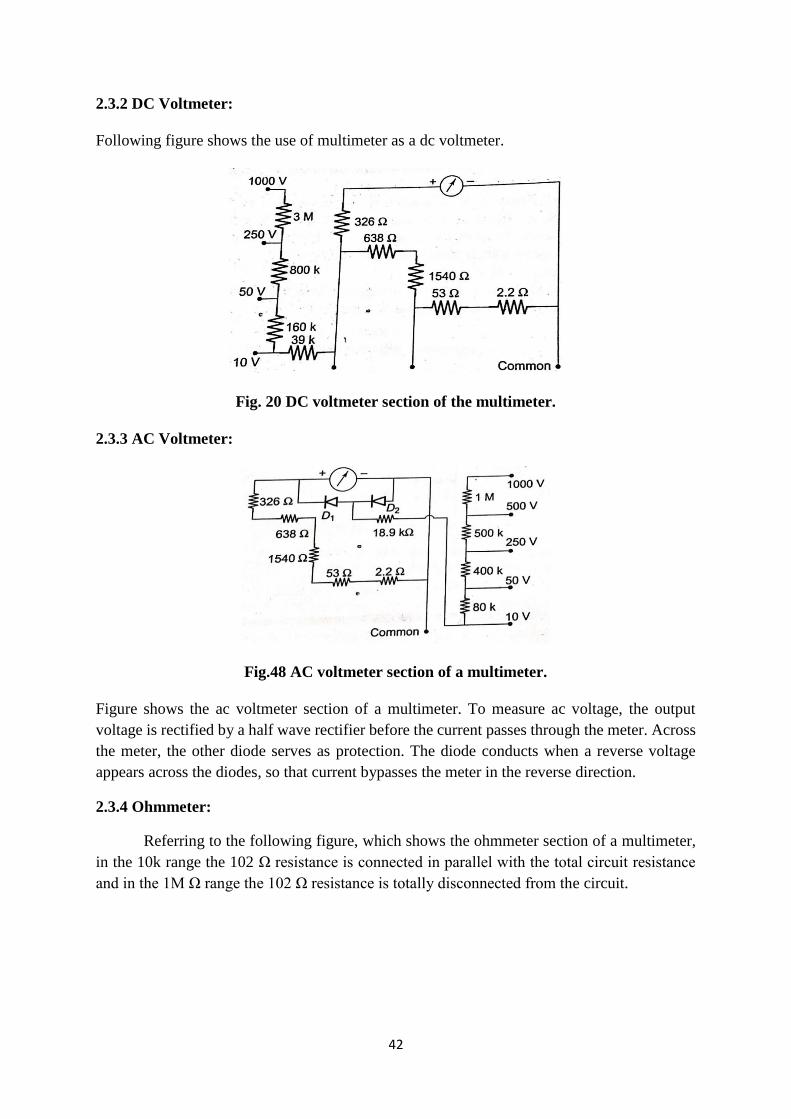
42

2.3.2 DC Voltmeter:

Following figure shows the use of multimeter as a dc voltmeter.

Fig. 20 DC voltmeter section of the multimeter.

2.3.3 AC Voltmeter:

Fig.48 AC voltmeter section of a multimeter.

Figure shows the ac voltmeter section of a multimeter. To measure ac voltage, the output

voltage is rectified by a half wave rectifier before the current passes through the meter. Across

the meter, the other diode serves as protection. The diode conducts when a reverse voltage

appears across the diodes, so that current bypasses the meter in the reverse direction.

2.3.4 Ohmmeter:

Referring to the following figure, which shows the ohmmeter section of a multimeter,

in the 10k range the 102 Ω resistance is connected in parallel with the total circuit resistance

and in the 1M Ω range the 102 Ω resistance is totally disconnected from the circuit.

43

Fig. 22: Ohmmeter section of the multimeter.

Therefore on the 1M Ω range, the half scale deflection is 10k. Since on the 10k range,

the 102 Ω resistance is joined across the total resistance, therefore in this range the half scale

deflection is 100 Ω. The measurement of resistance is done by applying a small voltage

installed within the meter. For the 1M Ω range, the internal resistance is 10k Ω. ie., value at the

mid scale.

Fig. 49 Equivalent resistance on the 1M Ω range and half scale deflection

The range of the ohmmeter can be changed by connecting the switch to a suitable shunt

resistance. By using different values of shunt resistance, different ranges can be obtained. By

increasing the battery voltage and using a suitable shunt, the maximum values which the

ohmmeter reads can be changed.

44

TYPES OF VOLTMETER

2.4 DIFFERENTIAL TYPE VOLTMETER

The differential voltmeter technique is one of the most common and accurate methods

of measuring unknown voltages. In this technique, the voltmeter is used to indicate the

difference between known and unknown voltages. ie., an unknown voltage is compared with a

known voltage.

Following figure shows the basic circuit of a differential voltmeter based on the

potentiometric method, hence the name potentiometric voltmeter.

Fig. 50 Basic Differential voltmeter.

In this method, the potentiometer is varied until the voltage across it equals the

unknown voltage, which is indicated by the null indicator reading zero. Under null conditions,

the meter draws current from neither the reference source nor the unknown voltage source and

hence the differential voltmeter represents an infinite impedance to the unknown source (The

null meter serves as an indicator only). To detect small differences the meter movement must

be sensitive but it need not be calibrated, since only zero has to be indicated. The reference

source used is usually a 1V dc standard source or a zener controlled precision supply. A high

voltage reference supply is used for measuring high voltages.

The usual practice, however is to employ voltage dividers or attenuators across an

unknown source to reduce the voltage. The input voltage divider has a relatively low input

impedance , especially for unknown voltages much higher than the reference standard. The

attenuation will have a loading effect and the input resistance of voltmeter is not infinity when

an attenuator is used.

In order to measure ac voltages, the ac voltages must be converted into dc by incorporating a

precision rectifier circuit. A block diagram of such ac differential voltmeter is shown below:

Fig. 51 Block diagram of an ac differential voltmeter.

45

2.4.1 True RMS Voltmeter

RMS value of the sinusoidal waveform is measured by the average reading voltmeter

of which scale is calibrated in terms of rms value. This method is quite simple and less

expensive. But sometimes rms value of the non-sinusoidal waveform is required to be

measured. For such a measurement a true rms reading voltmeter is required. True rms reading

voltmeter gives a meter indication by sensing heating power of waveform which is proportional

to the square of the rms value of the voltage.

Fig. 52 True RMS Voltmeter

Thermo-couple is used to measure the heating power of the input waveform of which

heater is supplied by the amplified version of the input waveform. Output voltage of the

thermocouple is proportional to the square of the rms value of the input waveform. One more

thermo-couple, called the balancing thermo-couple, is used in the same thermal environment

in order to overcome the difficulty arising out of non-linear behaviour of the thermo-couple.

Non-linearity of the input circuit thermo-couple is cancelled by the similar non-linear effects

of the balancing thermo-couple. These thermo-couples form part of a bridge in the input circuit

of a dc amplifier, as shown in block diagram.

AC waveform to be measured is applied to the heating element of the main thermo-

couple through an ac amplifier. Under absence of any input waveform, output of both thermo-

couples are equal so error signal, which is input to dc amplifier, is zero and therefore indicating

meter connected to the output of dc amplifier reads zero. But on the application of input

waveform, output of main thermo-couple upsets the balance and an error signal is produced,

which gets amplified by the dc amplifier and fedback to the heating element of the balancing

thermo-couple. This feedback current reduces the value of error signal and ultimately makes it

zero to obtain the balanced bridge condition. In this balanced condition, feedback current

supplied by the dc amplifier to the heating element of the balance thermo-couple is equal to the

ac current flowing in the heating element of main thermo-couple. Hence this direct current is

directly proportional to the rms value of the input ac voltage and is indicated by the meter

connected in the output of the dc amplifier. The PMMC meter may be calibrated to read the

rms voltage directly.

46

By this method, rms value of any voltage waveform can be measured provided that the peak

excursions of the waveform do not exceed the dynamic range of the ac amplifier.

2.4.2 Vector Voltmeter

The vector voltmeter is basically a new type of amplitude and phase measuring device.

It uses two samplers to sample the two waves whose amplitude and relative phase are to be

measured. It measures the voltages at two different points in the circuit and also measures the

phase difference between these voltages at these two points. In this voltmeter, two RF signals

of the same fundamental frequency (1MHz to GHz) are converted to two IF signals. The

amplitudes, waveforms and the phase relations of IF signals are same as that of RF signals.

Thus, the fundamental components of the IF signal have the same amplitude and phase

relationships as the fundamental components RF signals. These fundamental components are

filtered from the IF signals and are measured by a voltmeter and phase meter.

Fig. 53 Block diagram of Vector Voltmeter

The vector voltmeter is useful in VHF applications and are used as :

1)Insertion loses

2)Complex impedance of mixers

3)S parameters of transistors

4) Radio frequency distortion

5) Amplitude modulation index

6) Amplifier gain and phase shift

7) Filter transfer functions

47

8) Two port network parameters.

The block diagram shows the instrument consists of five major sections. Two IF-RF

converters, an automatic phase control section, a phase meter circuit, a voltmeter circuit. The

RF-IF converters and the phase control sections produce two 20KHz sine waves with the same

amplitudes and phase relationships as the fundamental components of the RF signals applied

to channels A and B. The phase meter section continuously monitor these two 20KHz sine

waves and indicates the phase angle between them. The voltmeter section can be switched to

channel A or channel B to provide a meter display of the amplitude.

Each RF-IF converter consists of a sampler and a tuned amplifier. The sampler

produces a 20 KHz replica of the input RF waveform, and the tuned amplifier extracts the

20KHz fundamental component from this waveform replica. The phase control unit is rather a

sophisticated circuit that generates the sampling pulses for both RF-IF converters and

automatically controls the pulse rate to produce 20KHz IF signals. The sampling pulse rate is

controlled by a voltage tuned oscillator (VTO) for which the tuning voltage is supplied by an

automatic phase control section. This section locks the IF signal of channel A to a 20KHz

reference oscillator. To get initial locking, the phase control section applies a ramp voltage to

the VTO. The ramp voltage sweeps the sampling rate until channel A IF is 20KHz and in phase

with the reference oscillator.

To determine the phase difference between the two IF signals, the tuned amplifiers are

followed by the phase meter circuit. Each channel is first amplified and then limited resulting

in square wave signals at the inputs to the IF phase shifting circuits. The circuit in channel A

shifts the phase of the square wave signal by +600 the circuit in channel B shifts the phase of

its signal by -1200 Both phase shifts are accomplished by a combination of capacitive networks

and inverting and non-inverting amplifiers whose vector-sum outputs provide the desired phase

shift. The outputs of the phase shift circuits are amplified and clipped, producing square

waveforms and applied to trigger amplifiers. These circuits convert the square wave input

signals to positive spikes with very fast rise times. The bistable multivibrator is triggered by

the pulses from both the channels, Channel A is joined to the set input of the MV, channel B is

joined to the reset input of the MV. If the initial phase shift between the RF signals at the probes

was 00, the trigger pulses into the multivibrator are 1800 out of phase owing to the action of the

phase shift circuits. The MV then produces a square wave output voltage which is symmetrical

about zero.

The instrument contains a power supply section, which is not shown in the block

diagram. The power supply generates all the needed supply voltages for the various sections of

the instrument.

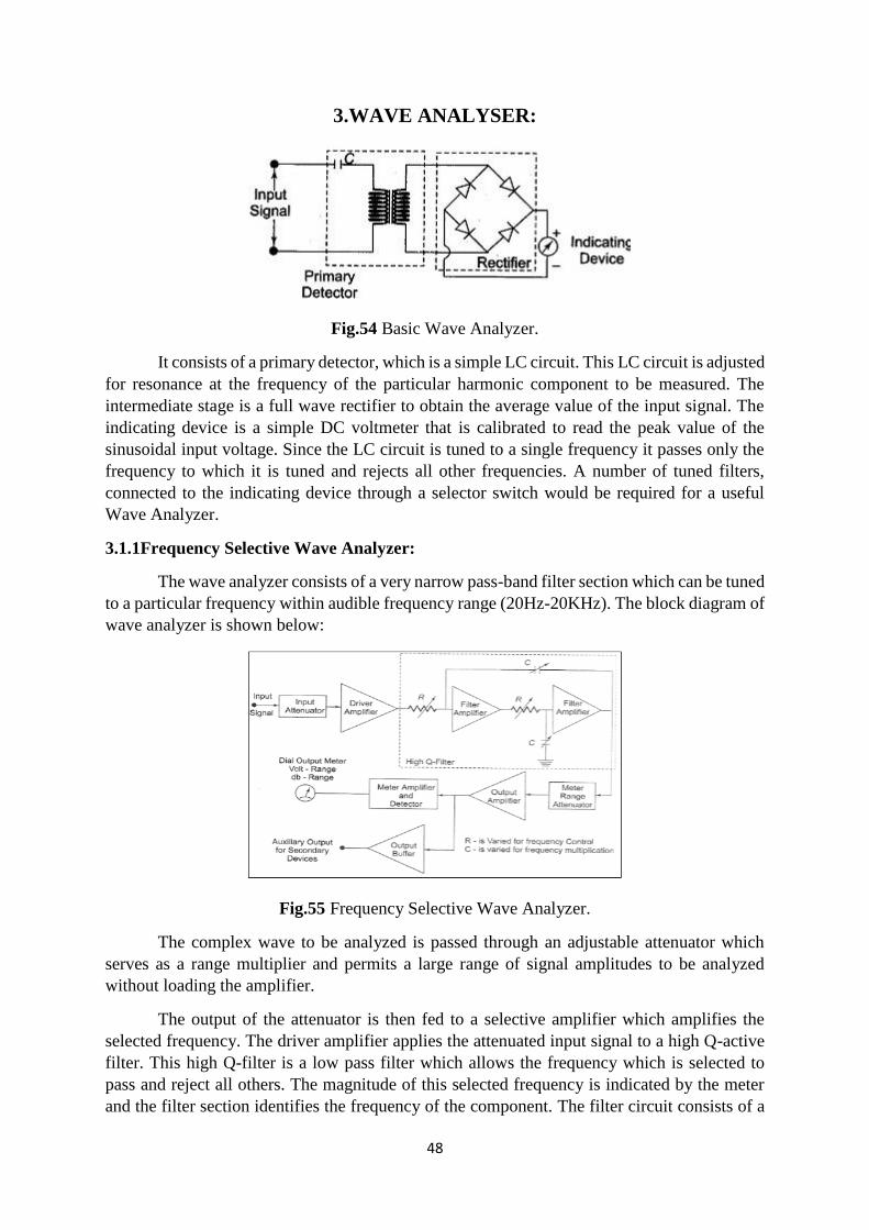
48

3.WAVE ANALYSER:

Fig.54 Basic Wave Analyzer.

It consists of a primary detector, which is a simple LC circuit. This LC circuit is adjusted

for resonance at the frequency of the particular harmonic component to be measured. The

intermediate stage is a full wave rectifier to obtain the average value of the input signal. The

indicating device is a simple DC voltmeter that is calibrated to read the peak value of the

sinusoidal input voltage. Since the LC circuit is tuned to a single frequency it passes only the

frequency to which it is tuned and rejects all other frequencies. A number of tuned filters,

connected to the indicating device through a selector switch would be required for a useful

Wave Analyzer.

3.1.1Frequency Selective Wave Analyzer:

The wave analyzer consists of a very narrow pass-band filter section which can be tuned

to a particular frequency within audible frequency range (20Hz-20KHz). The block diagram of

wave analyzer is shown below:

Fig.55 Frequency Selective Wave Analyzer.

The complex wave to be analyzed is passed through an adjustable attenuator which

serves as a range multiplier and permits a large range of signal amplitudes to be analyzed

without loading the amplifier.

The output of the attenuator is then fed to a selective amplifier which amplifies the

selected frequency. The driver amplifier applies the attenuated input signal to a high Q-active

filter. This high Q-filter is a low pass filter which allows the frequency which is selected to

pass and reject all others. The magnitude of this selected frequency is indicated by the meter

and the filter section identifies the frequency of the component. The filter circuit consists of a

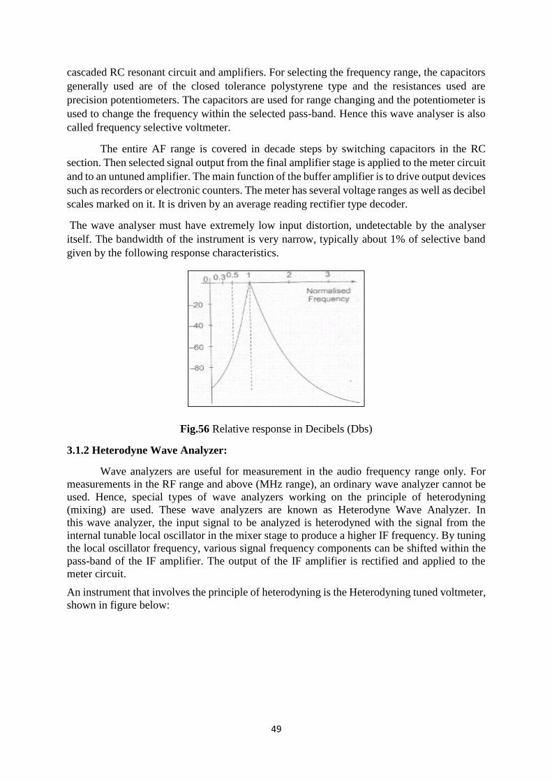
49

cascaded RC resonant circuit and amplifiers. For selecting the frequency range, the capacitors

generally used are of the closed tolerance polystyrene type and the resistances used are

precision potentiometers. The capacitors are used for range changing and the potentiometer is

used to change the frequency within the selected pass-band. Hence this wave analyser is also

called frequency selective voltmeter.

The entire AF range is covered in decade steps by switching capacitors in the RC

section. Then selected signal output from the final amplifier stage is applied to the meter circuit

and to an untuned amplifier. The main function of the buffer amplifier is to drive output devices

such as recorders or electronic counters. The meter has several voltage ranges as well as decibel

scales marked on it. It is driven by an average reading rectifier type decoder.

The wave analyser must have extremely low input distortion, undetectable by the analyser

itself. The bandwidth of the instrument is very narrow, typically about 1% of selective band

given by the following response characteristics.

Fig.56 Relative response in Decibels (Dbs)

3.1.2 Heterodyne Wave Analyzer:

Wave analyzers are useful for measurement in the audio frequency range only. For

measurements in the RF range and above (MHz range), an ordinary wave analyzer cannot be

used. Hence, special types of wave analyzers working on the principle of heterodyning

(mixing) are used. These wave analyzers are known as Heterodyne Wave Analyzer. In

this wave analyzer, the input signal to be analyzed is heterodyned with the signal from the

internal tunable local oscillator in the mixer stage to produce a higher IF frequency. By tuning

the local oscillator frequency, various signal frequency components can be shifted within the

pass-band of the IF amplifier. The output of the IF amplifier is rectified and applied to the

meter circuit.

An instrument that involves the principle of heterodyning is the Heterodyning tuned voltmeter,

shown in figure below:

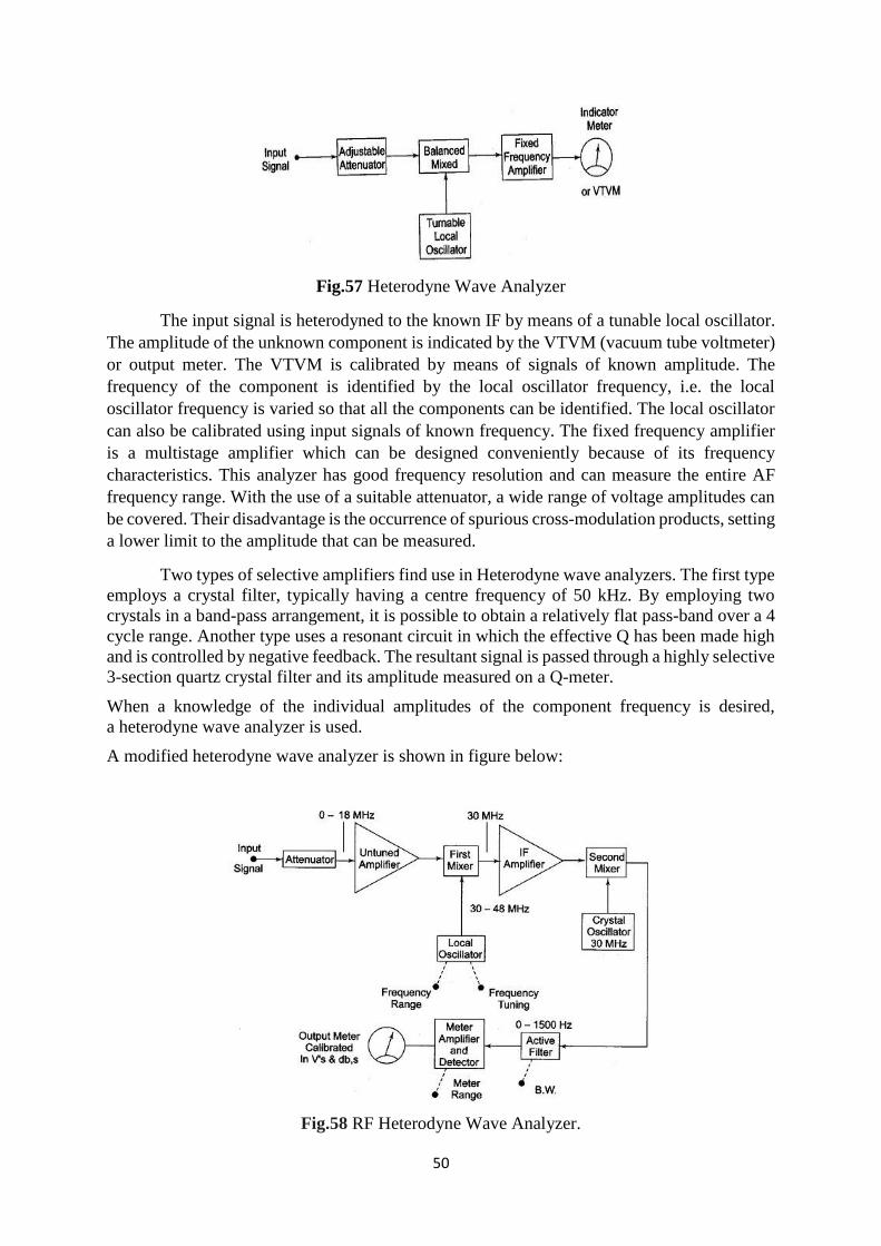
50

Fig.57 Heterodyne Wave Analyzer

The input signal is heterodyned to the known IF by means of a tunable local oscillator.

The amplitude of the unknown component is indicated by the VTVM (vacuum tube voltmeter)

or output meter. The VTVM is calibrated by means of signals of known amplitude. The

frequency of the component is identified by the local oscillator frequency, i.e. the local

oscillator frequency is varied so that all the components can be identified. The local oscillator

can also be calibrated using input signals of known frequency. The fixed frequency amplifier

is a multistage amplifier which can be designed conveniently because of its frequency

characteristics. This analyzer has good frequency resolution and can measure the entire AF

frequency range. With the use of a suitable attenuator, a wide range of voltage amplitudes can

be covered. Their disadvantage is the occurrence of spurious cross-modulation products, setting

a lower limit to the amplitude that can be measured.

Two types of selective amplifiers find use in Heterodyne wave analyzers. The first type

employs a crystal filter, typically having a centre frequency of 50 kHz. By employing two

crystals in a band-pass arrangement, it is possible to obtain a relatively flat pass-band over a 4

cycle range. Another type uses a resonant circuit in which the effective Q has been made high

and is controlled by negative feedback. The resultant signal is passed through a highly selective

3-section quartz crystal filter and its amplitude measured on a Q-meter.

When a knowledge of the individual amplitudes of the component frequency is desired,

a heterodyne wave analyzer is used.

A modified heterodyne wave analyzer is shown in figure below:

Fig.58 RF Heterodyne Wave Analyzer.

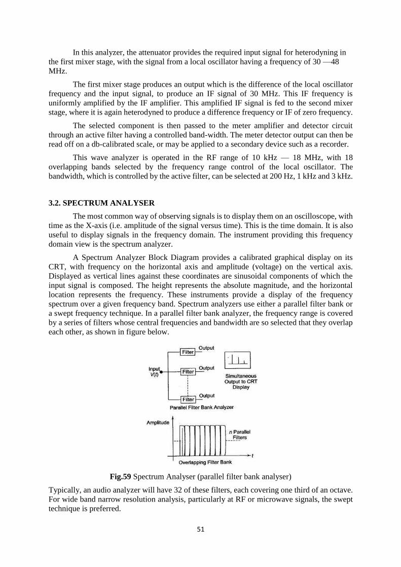
51

In this analyzer, the attenuator provides the required input signal for heterodyning in

the first mixer stage, with the signal from a local oscillator having a frequency of 30 —48

MHz.

The first mixer stage produces an output which is the difference of the local oscillator

frequency and the input signal, to produce an IF signal of 30 MHz. This IF frequency is

uniformly amplified by the IF amplifier. This amplified IF signal is fed to the second mixer

stage, where it is again heterodyned to produce a difference frequency or IF of zero frequency.

The selected component is then passed to the meter amplifier and detector circuit

through an active filter having a controlled band-width. The meter detector output can then be

read off on a db-calibrated scale, or may be applied to a secondary device such as a recorder.

This wave analyzer is operated in the RF range of 10 kHz — 18 MHz, with 18

overlapping bands selected by the frequency range control of the local oscillator. The

bandwidth, which is controlled by the active filter, can be selected at 200 Hz, 1 kHz and 3 kHz.

3.2. SPECTRUM ANALYSER

The most common way of observing signals is to display them on an oscilloscope, with

time as the X-axis (i.e. amplitude of the signal versus time). This is the time domain. It is also

useful to display signals in the frequency domain. The instrument providing this frequency

domain view is the spectrum analyzer.

A Spectrum Analyzer Block Diagram provides a calibrated graphical display on its

CRT, with frequency on the horizontal axis and amplitude (voltage) on the vertical axis.

Displayed as vertical lines against these coordinates are sinusoidal components of which the

input signal is composed. The height represents the absolute magnitude, and the horizontal

location represents the frequency. These instruments provide a display of the frequency

spectrum over a given frequency band. Spectrum analyzers use either a parallel filter bank or

a swept frequency technique. In a parallel filter bank analyzer, the frequency range is covered

by a series of filters whose central frequencies and bandwidth are so selected that they overlap

each other, as shown in figure below.

Fig.59 Spectrum Analyser (parallel filter bank analyser)

Typically, an audio analyzer will have 32 of these filters, each covering one third of an octave.

For wide band narrow resolution analysis, particularly at RF or microwave signals, the swept

technique is preferred.

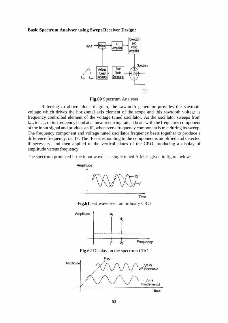
52

Basic Spectrum Analyser using Swept Receiver Design:

Fig.60 Spectrum Analyser

Referring to above block diagram, the sawtooth generator provides the sawtooth

voltage which drives the horizontal axis element of the scope and this sawtooth voltage is

frequency controlled element of the voltage tuned oscillator. As the oscillator sweeps from

fmin to fmax of its frequency band at a linear recurring rate, it beats with the frequency component

of the input signal and produce an IF, whenever a frequency component is met during its sweep.

The frequency component and voltage tuned oscillator frequency beats together to produce a

difference frequency, i.e. IF. The IF corresponding to the component is amplified and detected

if necessary, and then applied to the vertical plates of the CRO, producing a display of

amplitude versus frequency.

The spectrum produced if the input wave is a single tuned A.M. is given in figure below:

Fig.61Test wave seen on ordinary CRO

Fig.62 Display on the spectrum CRO

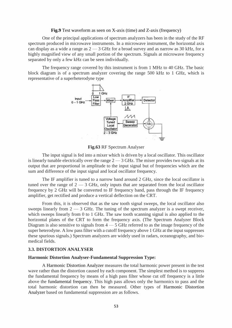
53

Fig.9 Test waveform as seen on X-axis (time) and Z-axis (frequency)

One of the principal applications of spectrum analyzers has been in the study of the RF

spectrum produced in microwave instruments. In a microwave instrument, the horizontal axis

can display as a wide a range as 2 — 3 GHz for a broad survey and as narrow as 30 kHz, for a

highly magnified view of any small portion of the spectrum. Signals at microwave frequency

separated by only a few kHz can be seen individually.

The frequency range covered by this instrument is from 1 MHz to 40 GHz. The basic

block diagram is of a spectrum analyzer covering the range 500 kHz to 1 GHz, which is

representative of a superheterodyne type

Fig.63 RF Spectrum Analyser

The input signal is fed into a mixer which is driven by a local oscillator. This oscillator

is linearly tunable electrically over the range 2 — 3 GHz. The mixer provides two signals at its

output that are proportional in amplitude to the input signal but of frequencies which are the

sum and difference of the input signal and local oscillator frequency.

The IF amplifier is tuned to a narrow band around 2 GHz, since the local oscillator is

tuned over the range of 2 — 3 GHz, only inputs that are separated from the local oscillator

frequency by 2 GHz will be converted to IF frequency band, pass through the IF frequency

amplifier, get rectified and produce a vertical deflection on the CRT.

From this, it is observed that as the saw tooth signal sweeps, the local oscillator also

sweeps linearly from 2 — 3 GHz. The tuning of the spectrum analyzer is a swept receiver,

which sweeps linearly from 0 to 1 GHz. The saw tooth scanning signal is also applied to the

horizontal plates of the CRT to form the frequency axis. (The Spectrum Analyzer Block

Diagram is also sensitive to signals from 4 — 5 GHz referred to as the image frequency of the

super heterodyne. A low pass filter with a cutoff frequency above 1 GHz at the input suppresses

these spurious signals.) Spectrum analyzers are widely used in radars, oceanography, and bio-

medical fields.

3.3. DISTORTION ANALYSER

Harmonic Distortion Analyser-Fundamental Suppression Type:

A Harmonic Distortion Analyzer measures the total harmonic power present in the test

wave rather than the distortion caused by each component. The simplest method is to suppress

the fundamental frequency by means of a high pass filter whose cut off frequency is a little

above the fundamental frequency. This high pass allows only the harmonics to pass and the

total harmonic distortion can then be measured. Other types of Harmonic Distortion

Analyzer based on fundamental suppression are as follows.

54

a)Employing a Resonance Bridge type:

The bridge shown in Figure below. This bridge is balanced for the fundamental

frequency, i.e. L and C are tuned to the fundamental frequency. The bridge is unbalanced for

the harmonics, i.e. only harmonic power will be available at the output terminal and can be

measured. If the fundamental frequency is changed, the bridge must be balanced again. If L

and C are fixed components, then this method is suitable only when the test wave has a fixed

frequency. Indicators can be thermocouples or square law VTVMs (vacuum tube voltmeters).

This indicates the rms value of all harmonics. When a continuous adjustment of the

fundamental frequency is desired, a Wien bridge system is employed.

Fig.64 Resonance Bridge

b)Wien's Bridge method:

The bridge is balanced for the fundamental frequency. The fundamental energy is

dissipated in the bridge circuit elements. Only the harmonic components reach the output

terminals. The harmonic distortion output can then be measured with a meter. For balance at

the fundamental frequency, C1,C2,C, R1=R2=R,R3=2R4.

Fig.65 Wien's Bridge method.

c)Bridged T-Network:

55

Fig.66 Bridge T-Network method.

Referring to figure below, the L and C’s are tuned to the fundamental frequency, and R

is adjusted to bypass fundamental frequency. The tank circuit being tuned to the fundamental

frequency, the fundamental energy will circulate in the tank and is bypassed by the resistance.

Only harmonic components will reach the output terminals and the distorted output can be

measured by the meter. The Q of the resonant circuit must be at least 3-5.

One way of using a bridge T-network is given in figure below. The switch S is first connected

to point A so that the attenuator is excluded and the bridge T-network is adjusted for full

suppression of the fundamental frequency, i.e. minimum output. Minimum output indicates

that the bridged T-network is tuned to the fundamental frequency and that the fundamental

frequency is fully suppressed.

Fig.67 Harmonic Distortion Analyser using Bridged-T-Network.

The switch is next connected to terminal B, i.e. the bridged T-network is excluded.

Attenuation is adjusted until the same reading is obtained on the meter. The attenuator reading

indicates the total rms distortion. Distortion measurement can also be obtained by means of

a wave analyzer, knowing the amplitude and the frequency of each component, the Harmonic

Distortion Analyzer can be calculated. However, distortion meters based on fundamental

suppression are simpler to design and less expensive than wave analyzers. The disadvantage is

that they give only the total distortion and not the amplitude of individual distortion

components.

Reference books

1. Sawhney A.K., “A Course in Electrical, Electronic measurement &

Instrumentation”, Dhanpat Rai & sons, 18th Edition, Reprint 2010.

2. Doebelin E.O., “Measurement System Applications and Design”, McGraw Hill,

5th Edition, 2004.

3. Jain R.K., “Mechanical and Industrial Measurements”, Khanna Publishers, 11th

edition, Reprint 2005.

4. Jones’ Instrument Technology, Instrumentation Systems, Edited by B.E.Noltingk,

Vol 4, 4th edition, ELBS, 1987.

5. Murthy D.V.S., “Transducers and Instrumentation”, Printice Hall of India, 13th

printing, 2006.

6. Gnanavadivel,“Measurements and Instrumentation”,Anuradha Publication, Second

Revised Edition 2011.

56

SCHOOL OF ELECTRICAL AND ELECTRONICS

DEPARTMENT OF ELECTRICAL AND ELECTRONICS

UNIT – V

MEASUREMENT AND INSTRUMENTATION – SIC 1203

UNIT :5

Introduction to ADC / DAC - Specifications, ADC Quantization Error, Types of ADC -

Flash, Counter, Successive Approximation, Dual-Slope types and Introduction to Delta-

Sigma, Types of DAC - Weighted-Resistor, 2R ladder and PWM.

I.DATA CONVERTERS AND CONNECTORS

1.1 ADC AND DAC SPECIFICATIONS

Resolution

The resolution of a DAC is the smallest change in the output of the DAC for any change

in digital input.i.e. if a input to DAC changes one bit, how much analog output has changed in full

scale deflection.

% resolution = [Step size / Full scale output (FSO)] * 100

In other way the resolution is the number of states into which the full scale output is

divided. i.e if a 8 bit DAC can resolve the FSO up to 255 levels. Each level of output is called step

size and for higher number of bits the resolution will be better.

% resolution = [1/(2N-1) *100]

Normally the resolution will be in milli volts.

Accuracy

The Accuracy of a DAC is the difference between output practical analog output to the

ideal expected output for a given digital input. The DAC is contains electronic components where

the gain plays a major role which can introduce gain error in the output. Due to the the full scale

output may differ compared to ideal one. For an example if a DAC of 10 V is said to have an

accuracy of 0.01% there will be 10mv output deviation. The another factor which implicates the

accuracy is the zero offset error i.e for a zero input the output of DAC reflects some offset value.

Conversion Speed

The conversion speed of the DAC is output analog value settling time period for a change

in the digital input. This is also called settling time period of DAC. Normally it will be micro

seconds and in some advanced micro controller DAC it may be nano seconds.

Monotonicity

The Digital to Analog Converter is said to be monotonic if its analog value is either

increasing or equal to previous value for an LSB change in input digital signal.

Offset/ Zero scale error:

An input code of zero may be expected to give 0V output. A small offset may be present

and the transfer characteristic does not pass through the origin.

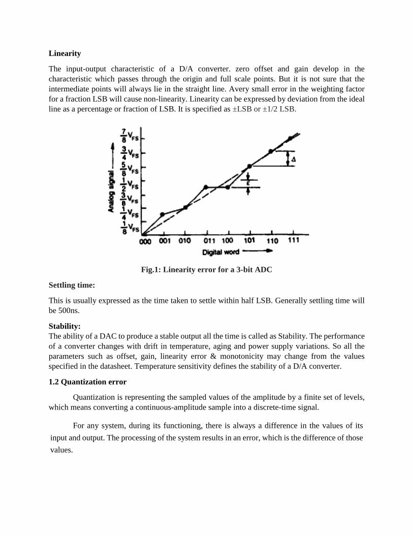
Linearity

The input-output characteristic of a D/A converter. zero offset and gain develop in the

characteristic which passes through the origin and full scale points. But it is not sure that the

intermediate points will always lie in the straight line. Avery small error in the weighting factor

for a fraction LSB will cause non-linearity. Linearity can be expressed by deviation from the ideal

line as a percentage or fraction of LSB. It is specified as ±LSB or ±1/2 LSB.

Fig.1: Linearity error for a 3-bit ADC

Settling time:

This is usually expressed as the time taken to settle within half LSB. Generally settling time will

be 500ns.

Stability:

The ability of a DAC to produce a stable output all the time is called as Stability. The performance

of a converter changes with drift in temperature, aging and power supply variations. So all the

parameters such as offset, gain, linearity error & monotonicity may change from the values

specified in the datasheet. Temperature sensitivity defines the stability of a D/A converter.

1.2 Quantization error

Quantization is representing the sampled values of the amplitude by a finite set of levels,

which means converting a continuous-amplitude sample into a discrete-time signal.

For any system, during its functioning, there is always a difference in the values of its

input and output. The processing of the system results in an error, which is the difference of those

values.

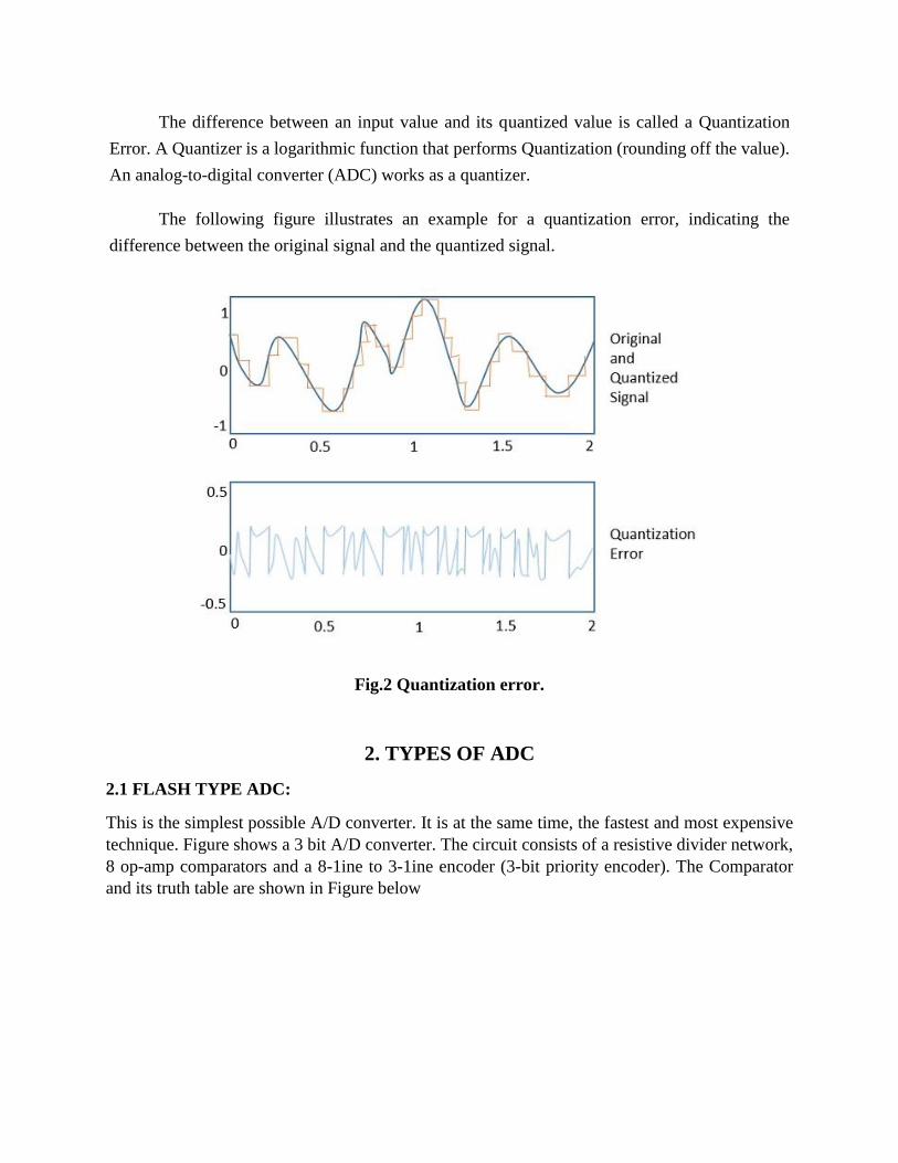
The difference between an input value and its quantized value is called a Quantization

Error. A Quantizer is a logarithmic function that performs Quantization (rounding off the value).

An analog-to-digital converter (ADC) works as a quantizer.

The following figure illustrates an example for a quantization error, indicating the

difference between the original signal and the quantized signal.

Fig.2 Quantization error.

2. TYPES OF ADC

2.1 FLASH TYPE ADC:

This is the simplest possible A/D converter. It is at the same time, the fastest and most expensive

technique. Figure shows a 3 bit A/D converter. The circuit consists of a resistive divider network,

8 op-amp comparators and a 8-1ine to 3-1ine encoder (3-bit priority encoder). The Comparator

and its truth table are shown in Figure below

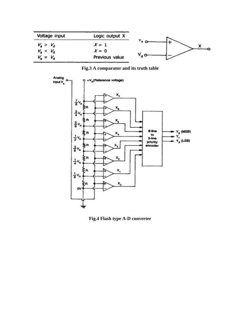
Fig.3 A comparator and its truth table

Fig.4 Flash type A-D converter

Table 1:Truth table for Flash type ADC

A small amount of hysteresis is built into the comparator to resolve any problems that might occur

if both inputs were of equal voltage as shown in the truth table. From the Figure, at each node of

the resistive divider, a comparison voltage is available. Since all the resistors are of equal value,

the voltage levels available at the nodes are equally divided between the reference voltage VR and

the ground. The purpose of the circuit is to compare the analog input voltage Va with each of the

node voltages. The truth table for the flash type A/D converter is shown above.

Advantages of flash type A/D converter

High speed simultaneous conversion

Typical conversion time is 100 ns or less.

Disadvantages of flash type A/D converter

The number of comparators required almost doubles for each added bit.

Larger the value of n (number of bits), the more complex is the priority encoder.

2.2 COUNTER TYPE ADC

The counter type ADC is the basic form of ADC which is also called as ramp type ADC

or stair case approximation ADC. This circuit consists of N-bit counter, DAC and comparator

Fig.5 Counter type ADC

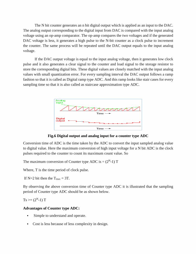
The N bit counter generates an n bit digital output which is applied as an input to the DAC.

The analog output corresponding to the digital input from DAC is compared with the input analog

voltage using an op-amp comparator. The op-amp compares the two voltages and if the generated

DAC voltage is less, it generates a high pulse to the N-bit counter as a clock pulse to increment

the counter. The same process will be repeated until the DAC output equals to the input analog

voltage.

If the DAC output voltage is equal to the input analog voltage, then it generates low clock

pulse and it also generates a clear signal to the counter and load signal to the storage resistor to

store the corresponding digital bits. These digital values are closely matched with the input analog

values with small quantization error. For every sampling interval the DAC output follows a ramp

fashion so that it is called as Digital ramp type ADC. And this ramp looks like stair cases for every

sampling time so that it is also called as staircase approximation type ADC.

Fig.6 Digital output and analog input for a counter type ADC

Conversion time of ADC is the time taken by the ADC to convert the input sampled analog value

to digital value. Here the maximum conversion of high input voltage for a N bit ADC is the clock

pulses required to the counter to count its maximum count value. So

The maximum conversion of Counter type ADC is = (2N-1) T

Where, T is the time period of clock pulse.

If N=2 bit then the Tmax = 3T.

By observing the above conversion time of Counter type ADC it is illustrated that the sampling

period of Counter type ADC should be as shown below.

Ts >= (2N-1) T

Advantages of Counter type ADC:

Simple to understand and operate.

Cost is less because of less complexity in design.

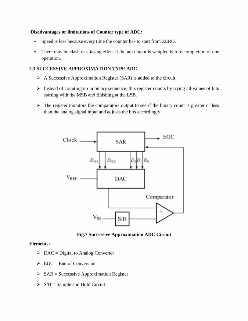
Disadvantages or limitations of Counter type of ADC:

Speed is less because every time the counter has to start from ZERO.

There may be clash or aliasing effect if the next input is sampled before completion of one

operation.

2.3 SUCCESSIVE APPROXIMATION TYPE ADC

A Successive Approximation Register (SAR) is added to the circuit

Instead of counting up in binary sequence, this register counts by trying all values of bits

starting with the MSB and finishing at the LSB.

The register monitors the comparators output to see if the binary count is greater or less

than the analog signal input and adjusts the bits accordingly

Fig.7 Successive Approximation ADC Circuit

Elements:

DAC = Digital to Analog Converter

EOC = End of Conversion

SAR = Successive Approximation Register

S/H = Sample and Hold Circuit

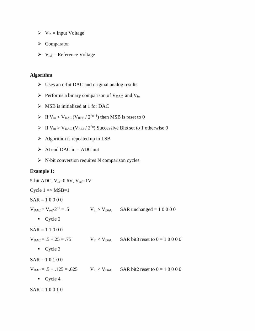
Vin = Input Voltage

Comparator

Vref = Reference Voltage

Algorithm

Uses an n-bit DAC and original analog results

Performs a binary comparison of VDAC and Vin

MSB is initialized at 1 for DAC

If Vin < VDAC (VREF / 2^n=1) then MSB is reset to 0

If Vin > VDAC (VREF / 2^n) Successive Bits set to 1 otherwise 0

Algorithm is repeated up to LSB

At end DAC in = ADC out

N-bit conversion requires N comparison cycles

Example 1:

5-bit ADC, Vin=0.6V, Vref=1V

Cycle 1 => MSB=1

SAR = 1 0 0 0 0

VDAC = Vref/2

^1 = .5 Vin > VDAC SAR unchanged = 1 0 0 0 0

Cycle 2

SAR = 1 1 0 0 0

VDAC = .5 +.25 = .75 Vin < VDAC SAR bit3 reset to 0 = 1 0 0 0 0

Cycle 3

SAR = 1 0 1 0 0

VDAC = .5 + .125 = .625 Vin < VDAC SAR bit2 reset to 0 = 1 0 0 0 0

Cycle 4

SAR = 1 0 0 1 0

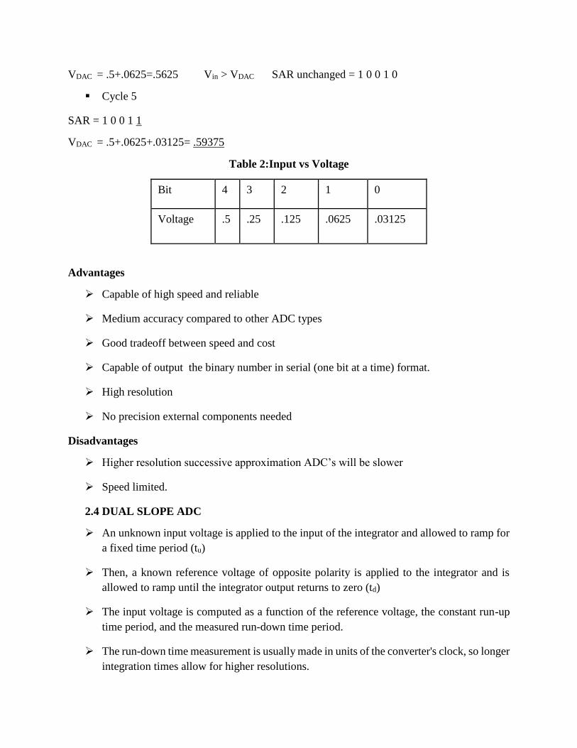
VDAC = .5+.0625=.5625 Vin > VDAC SAR unchanged = 1 0 0 1 0

Cycle 5

SAR = 1 0 0 1 1

VDAC = .5+.0625+.03125= .59375

Table 2:Input vs Voltage

Bit 4 3 2 1 0

Voltage .5 .25 .125 .0625 .03125

Advantages

Capable of high speed and reliable

Medium accuracy compared to other ADC types

Good tradeoff between speed and cost

Capable of output the binary number in serial (one bit at a time) format.

High resolution

No precision external components needed

Disadvantages

Higher resolution successive approximation ADC’s will be slower

Speed limited.

2.4 DUAL SLOPE ADC

An unknown input voltage is applied to the input of the integrator and allowed to ramp for

a fixed time period (tu)

Then, a known reference voltage of opposite polarity is applied to the integrator and is

allowed to ramp until the integrator output returns to zero (td)

The input voltage is computed as a function of the reference voltage, the constant run-up

time period, and the measured run-down time period.

The run-down time measurement is usually made in units of the converter's clock, so longer

integration times allow for higher resolutions.

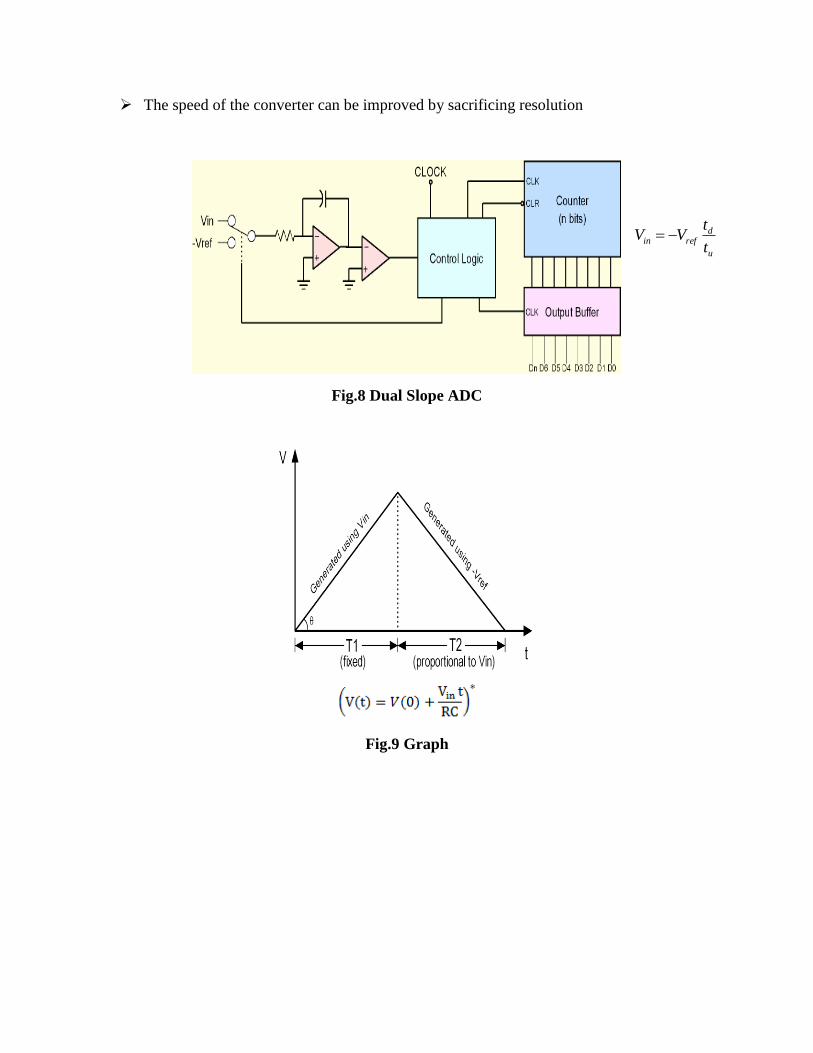
The speed of the converter can be improved by sacrificing resolution

Fig.8 Dual Slope ADC

Fig.9 Graph

u

drefin

t

tVV

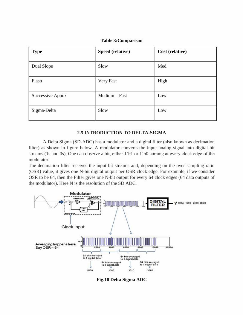
Table 3:Comparison

Type Speed (relative) Cost (relative)

Dual Slope Slow Med

Flash Very Fast High

Successive Appox Medium – Fast Low

Sigma-Delta Slow Low

2.5 INTRODUCTION TO DELTA-SIGMA

A Delta Sigma (SD-ADC) has a modulator and a digital filter (also known as decimation

filter) as shown in figure below. A modulator converts the input analog signal into digital bit

streams (1s and 0s). One can observe a bit, either 1’b1 or 1’b0 coming at every clock edge of the

modulator.

The decimation filter receives the input bit streams and, depending on the over sampling ratio

(OSR) value, it gives one N-bit digital output per OSR clock edge. For example, if we consider

OSR to be 64, then the Filter gives one N-bit output for every 64 clock edges (64 data outputs of

the modulator). Here N is the resolution of the SD ADC.

Fig.10 Delta Sigma ADC

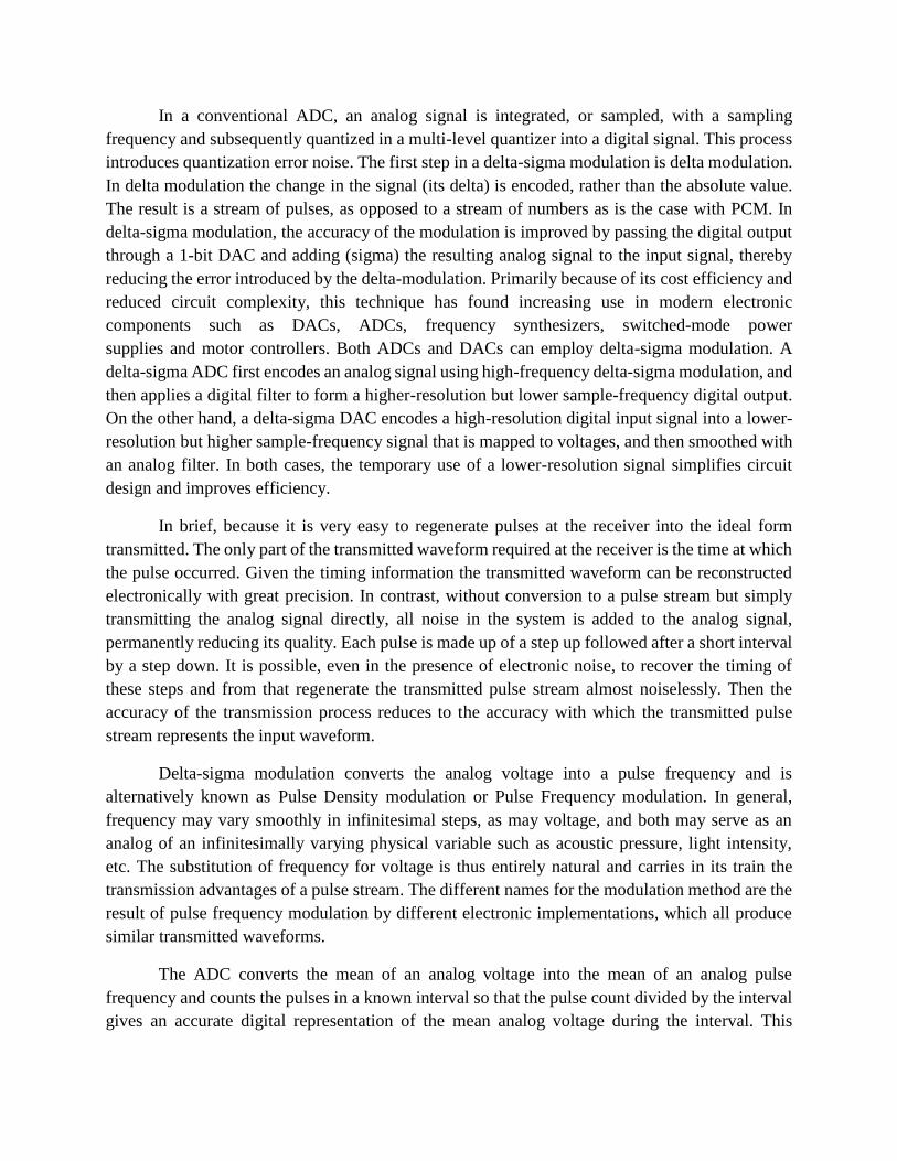
In a conventional ADC, an analog signal is integrated, or sampled, with a sampling

frequency and subsequently quantized in a multi-level quantizer into a digital signal. This process

introduces quantization error noise. The first step in a delta-sigma modulation is delta modulation.

In delta modulation the change in the signal (its delta) is encoded, rather than the absolute value.

The result is a stream of pulses, as opposed to a stream of numbers as is the case with PCM. In

delta-sigma modulation, the accuracy of the modulation is improved by passing the digital output

through a 1-bit DAC and adding (sigma) the resulting analog signal to the input signal, thereby

reducing the error introduced by the delta-modulation. Primarily because of its cost efficiency and

reduced circuit complexity, this technique has found increasing use in modern electronic

components such as DACs, ADCs, frequency synthesizers, switched-mode power

supplies and motor controllers. Both ADCs and DACs can employ delta-sigma modulation. A

delta-sigma ADC first encodes an analog signal using high-frequency delta-sigma modulation, and

then applies a digital filter to form a higher-resolution but lower sample-frequency digital output.

On the other hand, a delta-sigma DAC encodes a high-resolution digital input signal into a lower-

resolution but higher sample-frequency signal that is mapped to voltages, and then smoothed with

an analog filter. In both cases, the temporary use of a lower-resolution signal simplifies circuit

design and improves efficiency.

In brief, because it is very easy to regenerate pulses at the receiver into the ideal form

transmitted. The only part of the transmitted waveform required at the receiver is the time at which

the pulse occurred. Given the timing information the transmitted waveform can be reconstructed

electronically with great precision. In contrast, without conversion to a pulse stream but simply

transmitting the analog signal directly, all noise in the system is added to the analog signal,

permanently reducing its quality. Each pulse is made up of a step up followed after a short interval

by a step down. It is possible, even in the presence of electronic noise, to recover the timing of

these steps and from that regenerate the transmitted pulse stream almost noiselessly. Then the

accuracy of the transmission process reduces to the accuracy with which the transmitted pulse

stream represents the input waveform.

Delta-sigma modulation converts the analog voltage into a pulse frequency and is

alternatively known as Pulse Density modulation or Pulse Frequency modulation. In general,

frequency may vary smoothly in infinitesimal steps, as may voltage, and both may serve as an

analog of an infinitesimally varying physical variable such as acoustic pressure, light intensity,

etc. The substitution of frequency for voltage is thus entirely natural and carries in its train the

transmission advantages of a pulse stream. The different names for the modulation method are the

result of pulse frequency modulation by different electronic implementations, which all produce

similar transmitted waveforms.

The ADC converts the mean of an analog voltage into the mean of an analog pulse

frequency and counts the pulses in a known interval so that the pulse count divided by the interval

gives an accurate digital representation of the mean analog voltage during the interval. This

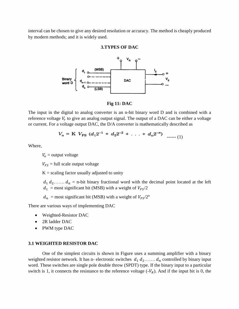
interval can be chosen to give any desired resolution or accuracy. The method is cheaply produced

by modern methods; and it is widely used.

3.TYPES OF DAC

Fig 11: DAC

The input in the digital to analog converter is an n-bit binary word D and is combined with a

reference voltage 𝑉𝑟 to give an analog output signal. The output of a DAC can be either a voltage

or current. For a voltage output DAC, the D/A converter is mathematically described as

------ (1)

Where,

𝑉𝑜 = output voltage

𝑉𝐹𝑆 = full scale output voltage

K = scaling factor usually adjusted to unity

𝑑1 𝑑2……. 𝑑𝑛 = n-bit binary fractional word with the decimal point located at the left

𝑑1 = most significant bit (MSB) with a weight of 𝑉𝐹𝑆/2

𝑑𝑛 = most significant bit (MSB) with a weight of 𝑉𝐹𝑆/2n

There are various ways of implementing DAC

Weighted-Resistor DAC

2R ladder DAC

PWM type DAC

3.1 WEIGHTED RESISTOR DAC

One of the simplest circuits is shown in Figure uses a summing amplifier with a binary

weighted resistor network. It has n- electronic switches 𝑑1 𝑑2……. 𝑑𝑛 controlled by binary input

word. These switches are single pole double throw (SPDT) type. If the binary input to a particular

switch is 1, it connects the resistance to the reference voltage (-𝑉𝑅). And if the input bit is 0, the

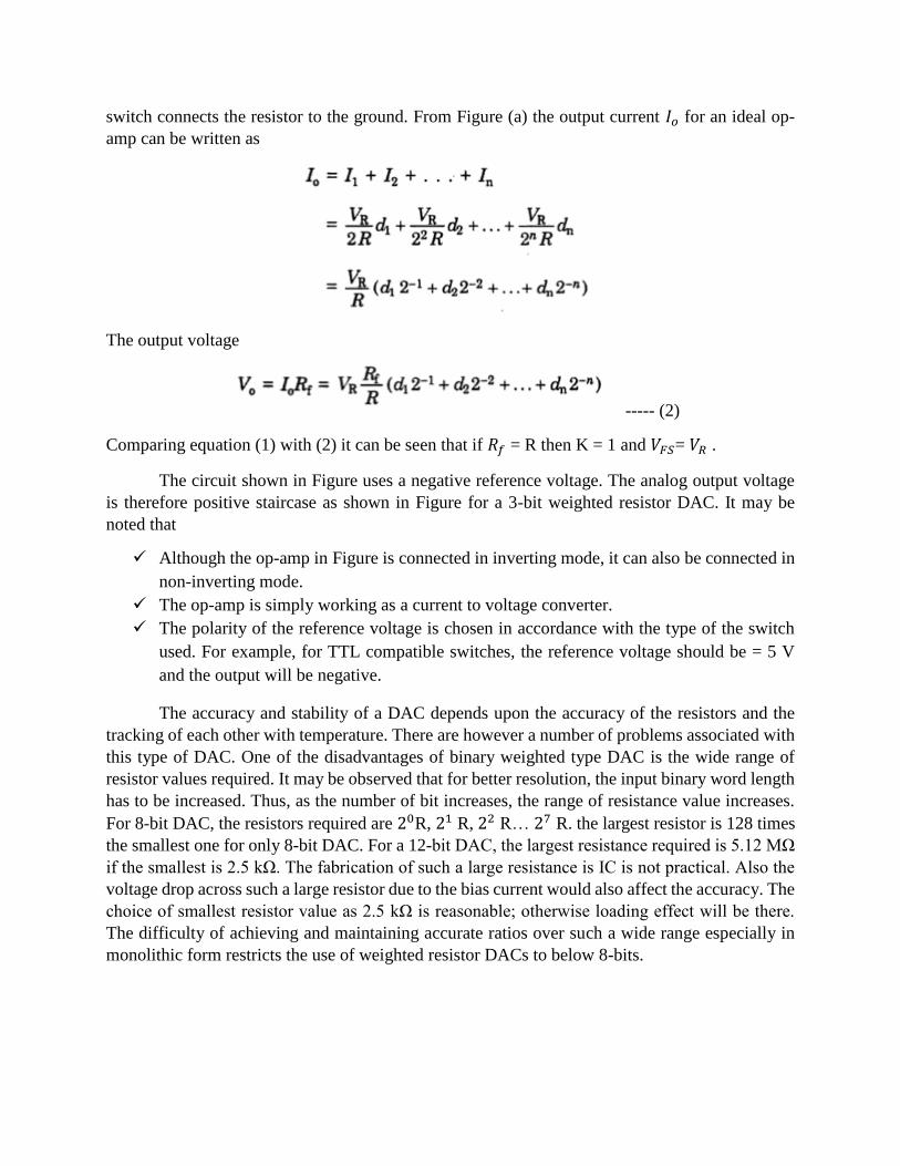
switch connects the resistor to the ground. From Figure (a) the output current 𝐼𝑜 for an ideal op-

amp can be written as

The output voltage

----- (2)

Comparing equation (1) with (2) it can be seen that if 𝑅𝑓 = R then K = 1 and 𝑉𝐹𝑆= 𝑉𝑅 .

The circuit shown in Figure uses a negative reference voltage. The analog output voltage

is therefore positive staircase as shown in Figure for a 3-bit weighted resistor DAC. It may be

noted that

Although the op-amp in Figure is connected in inverting mode, it can also be connected in

non-inverting mode.

The op-amp is simply working as a current to voltage converter.

The polarity of the reference voltage is chosen in accordance with the type of the switch

used. For example, for TTL compatible switches, the reference voltage should be = 5 V

and the output will be negative.

The accuracy and stability of a DAC depends upon the accuracy of the resistors and the

tracking of each other with temperature. There are however a number of problems associated with

this type of DAC. One of the disadvantages of binary weighted type DAC is the wide range of

resistor values required. It may be observed that for better resolution, the input binary word length

has to be increased. Thus, as the number of bit increases, the range of resistance value increases.

For 8-bit DAC, the resistors required are 20R, 21 R, 22 R… 27 R. the largest resistor is 128 times

the smallest one for only 8-bit DAC. For a 12-bit DAC, the largest resistance required is 5.12 MΩ

if the smallest is 2.5 kΩ. The fabrication of such a large resistance is IC is not practical. Also the

voltage drop across such a large resistor due to the bias current would also affect the accuracy. The

choice of smallest resistor value as 2.5 kΩ is reasonable; otherwise loading effect will be there.

The difficulty of achieving and maintaining accurate ratios over such a wide range especially in

monolithic form restricts the use of weighted resistor DACs to below 8-bits.

Fig.12 (a)A simple weighted resistor DAC (b) Transfer characteristics of a 3-bit DAC

3.2 R-2R LADDER DAC

Wide range of resistors are required in binary weighted resistor type DAC. This can be

avoided by using R-2R ladder type DAC where only two values of resistors are required. It is well

suited for integrated circuit realization. The typical value of resistor ranges from 2.5kΩ to 10kΩ.

For simplicity, consider a 3-bit DAC as shown in Figure, where the switch position

𝑑1 𝑑2 𝑑3 corresponds to the binary word 100. The circuit can be simplified to the equivalent form

of Figure (b) and finally to Figure (c). then, voltage at node C can be easily calculated by the set

procedure of network analysis as

Fig.13 (a) R-2R ladder DAC (b) Equivalent circuit of (a), (c) Equivalent circuit of (b)

The output voltage

The switch position corresponding to the binary word 001 in 3 bit DAC is shown in Figure

(a). The circuit can be simplified to the equivalent form of Fig(b). The voltages at the nodes

(A,B,C) formed by resistor branches are easily calculated in a similar fashion and the output

voltage becomes

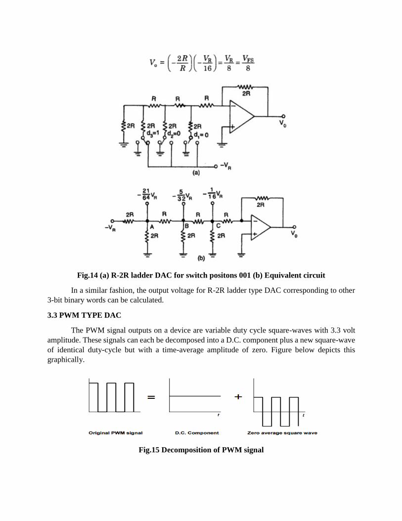
Fig.14 (a) R-2R ladder DAC for switch positons 001 (b) Equivalent circuit

In a similar fashion, the output voltage for R-2R ladder type DAC corresponding to other

3-bit binary words can be calculated.

3.3 PWM TYPE DAC

The PWM signal outputs on a device are variable duty cycle square-waves with 3.3 volt

amplitude. These signals can each be decomposed into a D.C. component plus a new square-wave

of identical duty-cycle but with a time-average amplitude of zero. Figure below depicts this

graphically.

Fig.15 Decomposition of PWM signal

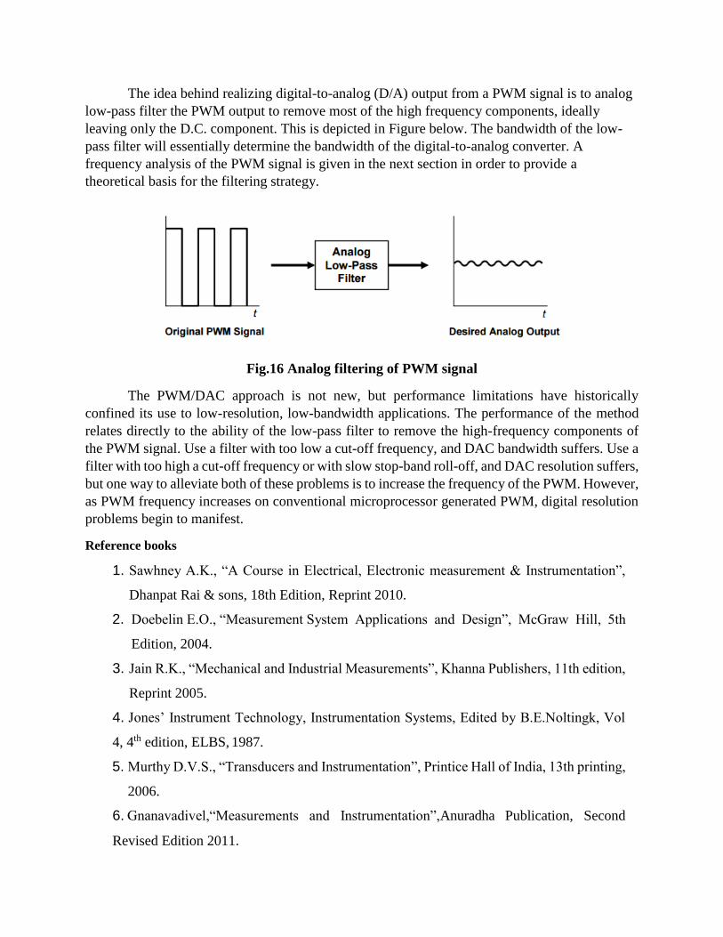
The idea behind realizing digital-to-analog (D/A) output from a PWM signal is to analog

low-pass filter the PWM output to remove most of the high frequency components, ideally

leaving only the D.C. component. This is depicted in Figure below. The bandwidth of the low-

pass filter will essentially determine the bandwidth of the digital-to-analog converter. A

frequency analysis of the PWM signal is given in the next section in order to provide a

theoretical basis for the filtering strategy.

Fig.16 Analog filtering of PWM signal

The PWM/DAC approach is not new, but performance limitations have historically

confined its use to low-resolution, low-bandwidth applications. The performance of the method

relates directly to the ability of the low-pass filter to remove the high-frequency components of

the PWM signal. Use a filter with too low a cut-off frequency, and DAC bandwidth suffers. Use a

filter with too high a cut-off frequency or with slow stop-band roll-off, and DAC resolution suffers,

but one way to alleviate both of these problems is to increase the frequency of the PWM. However,

as PWM frequency increases on conventional microprocessor generated PWM, digital resolution

problems begin to manifest.

Reference books

1. Sawhney A.K., “A Course in Electrical, Electronic measurement & Instrumentation”,

Dhanpat Rai & sons, 18th Edition, Reprint 2010.

2. Doebelin E.O., “Measurement System Applications and Design”, McGraw Hill, 5th

Edition, 2004.

3. Jain R.K., “Mechanical and Industrial Measurements”, Khanna Publishers, 11th edition,

Reprint 2005.

4. Jones’ Instrument Technology, Instrumentation Systems, Edited by B.E.Noltingk, Vol

4, 4th edition, ELBS, 1987.

5. Murthy D.V.S., “Transducers and Instrumentation”, Printice Hall of India, 13th printing,

2006.

6. Gnanavadivel,“Measurements and Instrumentation”,Anuradha Publication, Second

Revised Edition 2011.