unit 6: fractional factorial experiments at three levelsjeffwu/isye6413/unit_06_12spring.pdf ·...
TRANSCRIPT
Unit 6: Fractional Factorial Experiments at Three
Levels
Source : Chapter 6 (Sections 6.1 - 6.6)
• Larger-the-better and smaller-the-better problems.
• Basic concepts for 3k full factorial designs.
• Analysis of 3k designs using orthogonal components system.
• Design of 3-level fractional factorials.
• Effect aliasing, resolution and minimum aberration in 3k−p fractional
factorial designs.
• An alternative analysis method using linear-quadratic system.
1

Seat Belt Experiment• An experiment to study the effect of four factors on the pull strength of
truck seat belts.
• Four factors, each at three levels (Table 1).
• Two responses : crimp tensile strength that must be at least 4000 lb and flashthat cannot exceed 14 mm.
• 27 runs were conducted; each run was replicated three times as shown inTable 2.
Table 1: Factors and Levels, Seat-Belt Experiment
Level
Factor 0 1 2
A. pressure (psi) 1100 1400 1700
B. die flat (mm) 10.0 10.2 10.4
C. crimp length (mm) 18 23 27
D. anchor lot (#) P74 P75 P76
2

Design Matrix and Response Data, Seat-Belt
Experiment
Table 2: Design Matrix and Response Data, Seat-Belt Experiment: first 14 runs
Factor
Run A B C D Strength Flash
1 0 0 0 0 5164 6615 5959 12.89 12.70 12.74
2 0 0 1 1 5356 6117 5224 12.83 12.73 13.07
3 0 0 2 2 3070 3773 4257 12.37 12.47 12.44
4 0 1 0 1 5547 6566 6320 13.29 12.86 12.70
5 0 1 1 2 4754 4401 5436 12.64 12.50 12.61
6 0 1 2 0 5524 4050 4526 12.76 12.72 12.94
7 0 2 0 2 5684 6251 6214 13.17 13.33 13.98
8 0 2 1 0 5735 6271 5843 13.02 13.11 12.67
9 0 2 2 1 5744 4797 5416 12.37 12.67 12.54
10 1 0 0 1 6843 6895 6957 13.28 13.65 13.58
11 1 0 1 2 6538 6328 4784 12.62 14.07 13.38
12 1 0 2 0 6152 5819 5963 13.19 12.94 13.15
13 1 1 0 2 6854 6804 6907 14.65 14.98 14.40
14 1 1 1 0 6799 6703 6792 13.00 13.35 12.87
3
Design Matrix and Response Data, Seat-Belt
Experiment (contd.)
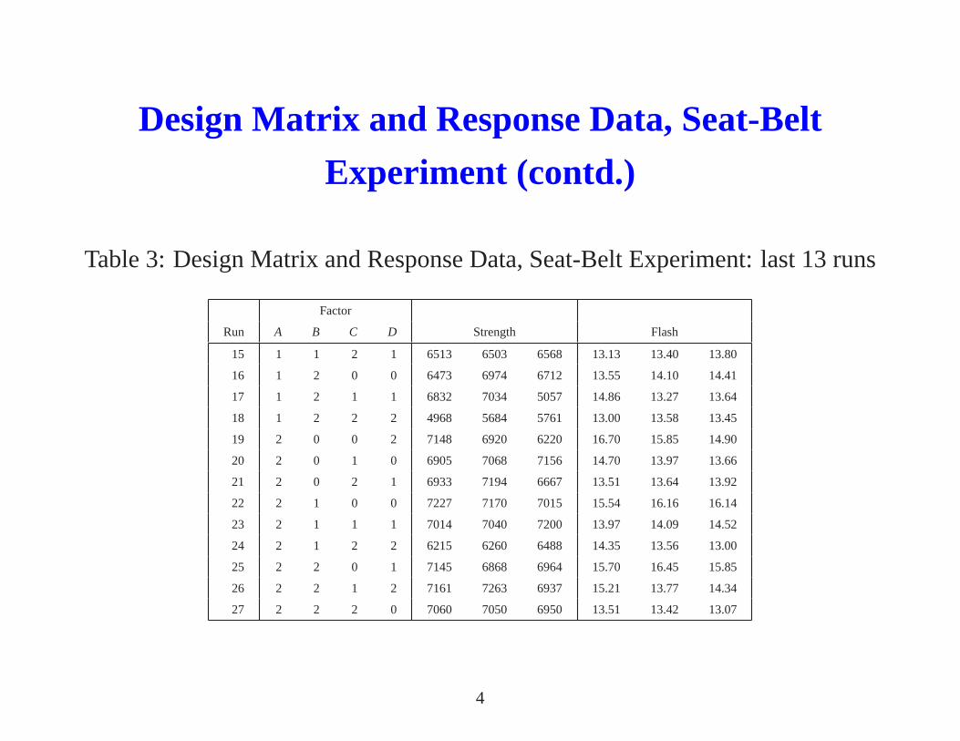
Table 3: Design Matrix and Response Data, Seat-Belt Experiment: last 13 runs
Factor
Run A B C D Strength Flash
15 1 1 2 1 6513 6503 6568 13.13 13.40 13.80
16 1 2 0 0 6473 6974 6712 13.55 14.10 14.41
17 1 2 1 1 6832 7034 5057 14.86 13.27 13.64
18 1 2 2 2 4968 5684 5761 13.00 13.58 13.45
19 2 0 0 2 7148 6920 6220 16.70 15.85 14.90
20 2 0 1 0 6905 7068 7156 14.70 13.97 13.66
21 2 0 2 1 6933 7194 6667 13.51 13.64 13.92
22 2 1 0 0 7227 7170 7015 15.54 16.16 16.14
23 2 1 1 1 7014 7040 7200 13.97 14.09 14.52
24 2 1 2 2 6215 6260 6488 14.35 13.56 13.00
25 2 2 0 1 7145 6868 6964 15.70 16.45 15.85
26 2 2 1 2 7161 7263 6937 15.21 13.77 14.34
27 2 2 2 0 7060 7050 6950 13.51 13.42 13.07
4

Larger-The-Better and Smaller-The-Better
problems
• In the seat-belt experiment, the strength should be as high as possible and the flash as
low as possible.
• There is no fixed nominal value for either strength or flash. Such type of problems
are referred to aslarger-the-better andsmaller-the-betterproblems, respectively.
• For such problems increasing or decreasing the mean is more difficult than reducing
the variation and should be done in the first step. (why?)
• Two-step procedure for larger-the-better problems:
1. Find factor settings that maximize E(y).
2. Find other factor settings that minimize Var(y).
• Two-step procedure for smaller-the-better problems:
1. Find factor settings that minimize E(y).
2. Find other factor settings that minimize Var(y).
5

Situations where three-level experiments are useful
• When there is a curvilinear relation between the response and a quantitative
factor like temperature. It is not possible to detect such a curvature effect
with two levels.
• A qualitative factor may have three levels (e.g., three types of machines or
three suppliers).
• It is common to study the effect of a factor on the response at its current
settingx0 and two settings aroundx0.
6
Analysis of3k designs using ANOVA
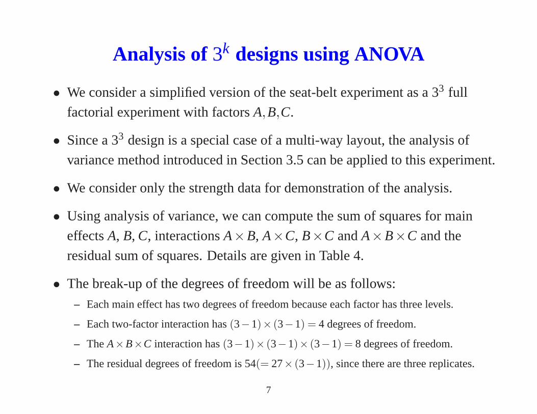
• We consider a simplified version of the seat-belt experimentas a 33 full
factorial experiment with factorsA,B,C.
• Since a 33 design is a special case of a multi-way layout, the analysis of
variance method introduced in Section 3.5 can be applied to this experiment.
• We consider only the strength data for demonstration of the analysis.
• Using analysis of variance, we can compute the sum of squaresfor main
effectsA, B, C, interactionsA×B, A×C, B×C andA×B×C and the
residual sum of squares. Details are given in Table 4.
• The break-up of the degrees of freedom will be as follows:
– Each main effect has two degrees of freedom because each factor has three levels.
– Each two-factor interaction has(3−1)× (3−1) = 4 degrees of freedom.
– TheA×B×C interaction has(3−1)× (3−1)× (3−1) = 8 degrees of freedom.
– The residual degrees of freedom is 54(= 27× (3−1)), since there are three replicates.
7
Analysis of Simplified Seat-Belt Experiment
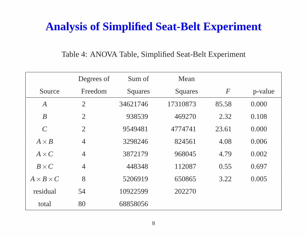
Table 4: ANOVA Table, Simplified Seat-Belt Experiment
Degrees of Sum of Mean
Source Freedom Squares Squares F p-value
A 2 34621746 17310873 85.58 0.000
B 2 938539 469270 2.32 0.108
C 2 9549481 4774741 23.61 0.000
A×B 4 3298246 824561 4.08 0.006
A×C 4 3872179 968045 4.79 0.002
B×C 4 448348 112087 0.55 0.697
A×B×C 8 5206919 650865 3.22 0.005
residual 54 10922599 202270
total 80 68858056
8

Orthogonal Components System: Decomposition of
A×B Interaction
• A×B has 4 degrees of freedom.
• A×B has two components denoted byABandAB2, each having 2 df.
• Let the levels ofA andB be denoted byx1 andx2 respectively.
• AB represents the contrasts among the response values whosex1 andx2
satisfy
x1 +x2 = 0,1,2(mod3),
• AB2 represents the contrasts among the response values whosex1 andx2
satisfy
x1 +2x2 = 0,1,2(mod3).
9

Orthogonal Components System: Decomposition of
A×B×C Interaction
• A×B×C has 8 degrees of freedom.
• It can be further split up into four components denoted byABC, ABC2,
AB2C andAB2C2, each having 2 df.
• Let the levels ofA, B andC be denoted byx1, x2 andx3 respectively.
• ABC, ABC2, AB2C andAB2C2 represent the contrasts among the three
groups of(x1,x2,x3) satisfying each of the four systems of equations,
x1 +x2 +x3 = 0,1,2(mod3),
x1 +x2 +2x3 = 0,1,2(mod3),
x1 +2x2 +x3 = 0,1,2(mod3),
x1 +2x2 +2x3 = 0,1,2(mod3).
10
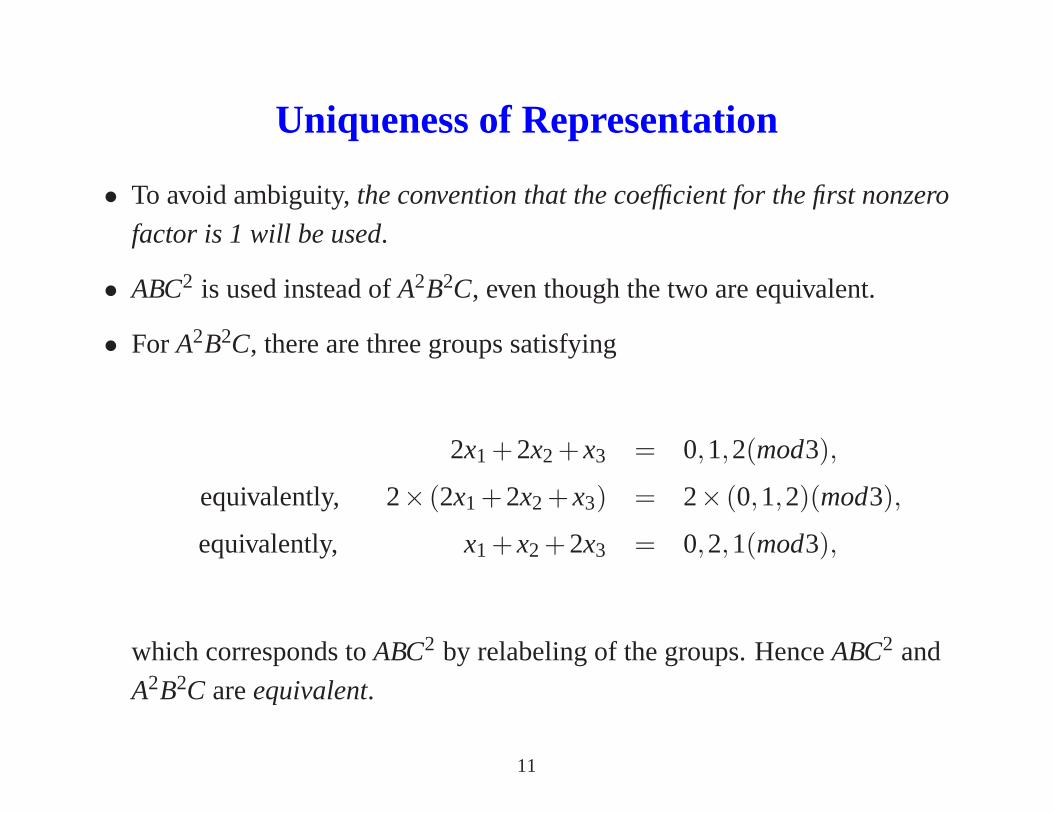
Uniqueness of Representation
• To avoid ambiguity,the convention that the coefficient for the first nonzero
factor is 1 will be used.
• ABC2 is used instead ofA2B2C, even though the two are equivalent.
• ForA2B2C, there are three groups satisfying
2x1 +2x2 +x3 = 0,1,2(mod3),
equivalently, 2× (2x1 +2x2 +x3) = 2× (0,1,2)(mod3),
equivalently, x1 +x2 +2x3 = 0,2,1(mod3),
which corresponds toABC2 by relabeling of the groups. HenceABC2 and
A2B2C areequivalent.
11

Representation ofABand AB2
Table 5: FactorA andB Combinations (x1 denotes the levels of factor A andx2
denotes the levels of factor B)
x2x1 0 1 2
0 αi (y00) βk (y01) γ j (y02)
1 β j (y10) γi (y11) αk (y12)
2 γk (y20) α j (y21) βi (y22)
• α,β,γ correspond to(x1,x2) with x1 +x2 = 0,1,2(mod3) resp.
• i, j,k correspond to(x1,x2) with x1 +2x2 = 0,1,2(mod3) resp.
12
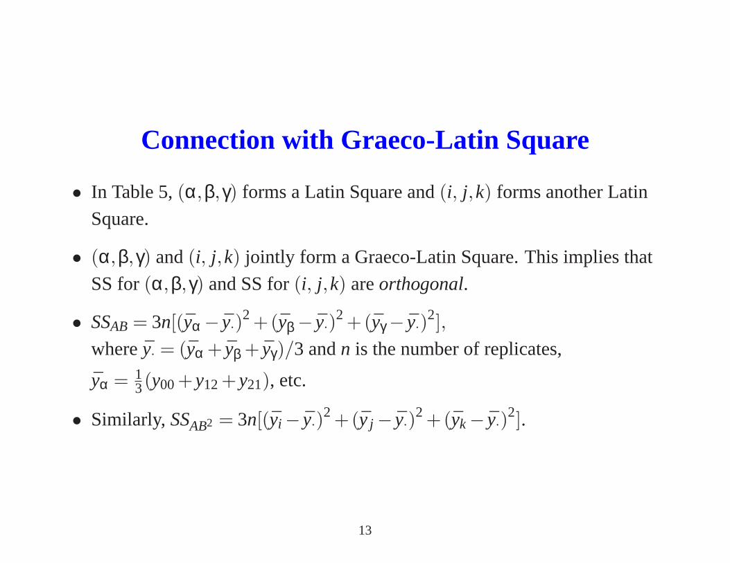
Connection with Graeco-Latin Square
• In Table 5,(α,β,γ) forms a Latin Square and(i, j,k) forms another Latin
Square.
• (α,β,γ) and(i, j,k) jointly form a Graeco-Latin Square. This implies that
SS for(α,β,γ) and SS for(i, j,k) areorthogonal.
• SSAB = 3n[(yα − y·)2 +(yβ − y·)
2 +(yγ − y·)2],
wherey· = (yα + yβ + yγ)/3 andn is the number of replicates,
yα = 13(y00+y12+y21), etc.
• Similarly, SSAB2 = 3n[(yi − y·)2 +(y j − y·)
2 +(yk− y·)2].
13

Analysis using the Orthogonal components system
• For the simplified seat-belt experiment, ¯yα = 6024.407,yβ = 6177.815 and
yγ = 6467.0, so that ¯y· = 6223.074 and
SSAB = (3)(9)[(6024.407−6223.074)2 +(6177.815−6223.074)2
+(6467.0−6223.074)2] = 2727451.
• Similarly, SSAB2 = 570795.
• See ANOVA table on the next page.
14

ANOVA : Simplified Seat-Belt Experiment
Degrees of Sum of Mean
Source Freedom Squares Squares F p-value
A 2 34621746 17310873 85.58 0.000
B 2 938539 469270 2.32 0.108
C 2 9549481 4774741 23.61 0.000
A×B 4 3298246 824561 4.08 0.006
AB 2 2727451 1363725 6.74 0.002
AB2 2 570795 285397 1.41 0.253
A×C 4 3872179 968045 4.79 0.002
AC 2 2985591 1492796 7.38 0.001
AC2 2 886587 443294 2.19 0.122
B×C 4 448348 112087 0.55 0.697
BC 2 427214 213607 1.06 0.355
BC2 2 21134 10567 0.05 0.949
A×B×C 8 5206919 650865 3.22 0.005
ABC 2 4492927 2246464 11.11 0.000
ABC2 2 263016 131508 0.65 0.526
AB2C 2 205537 102768 0.51 0.605
AB2C2 2 245439 122720 0.61 0.549
residual 54 10922599 202270
total 80 68858056
15

Analysis of Simplified Seat-Belt Experiment (contd)
• The significant main effects areA andC.
• Among the interactions,A×B, A×C andA×B×C are significant.
• We have difficulty in interpretations when only one component of the
interaction terms become significant. What is meant by “A×B is
significant”?
– HereAB is significant butAB2 is not.
– Is A×B significant because of the significance ofABalone ?
– For the original Seat-Belt Experiment, we haveAB= CD2.
• Similarly, AC is significant, but notAC2. How to interpret the significance of
A×C ?
• This difficulty in interpreting the significant interactioneffects can be
avoided by using Linear-Quadratic Systems.
16
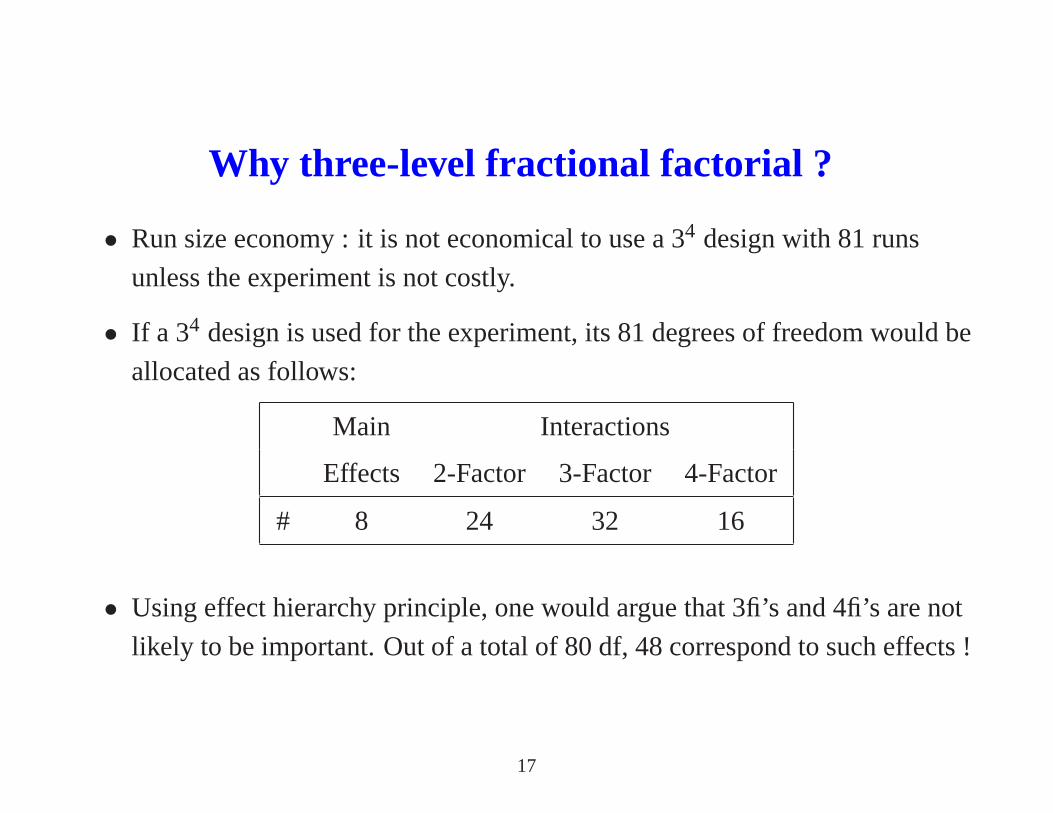
Why three-level fractional factorial ?
• Run size economy : it is not economical to use a 34 design with 81 runs
unless the experiment is not costly.
• If a 34 design is used for the experiment, its 81 degrees of freedom would be
allocated as follows:
Main Interactions
Effects 2-Factor 3-Factor 4-Factor
# 8 24 32 16
• Using effect hierarchy principle, one would argue that 3fi’sand 4fi’s are not
likely to be important. Out of a total of 80 df, 48 correspond to such effects !
17
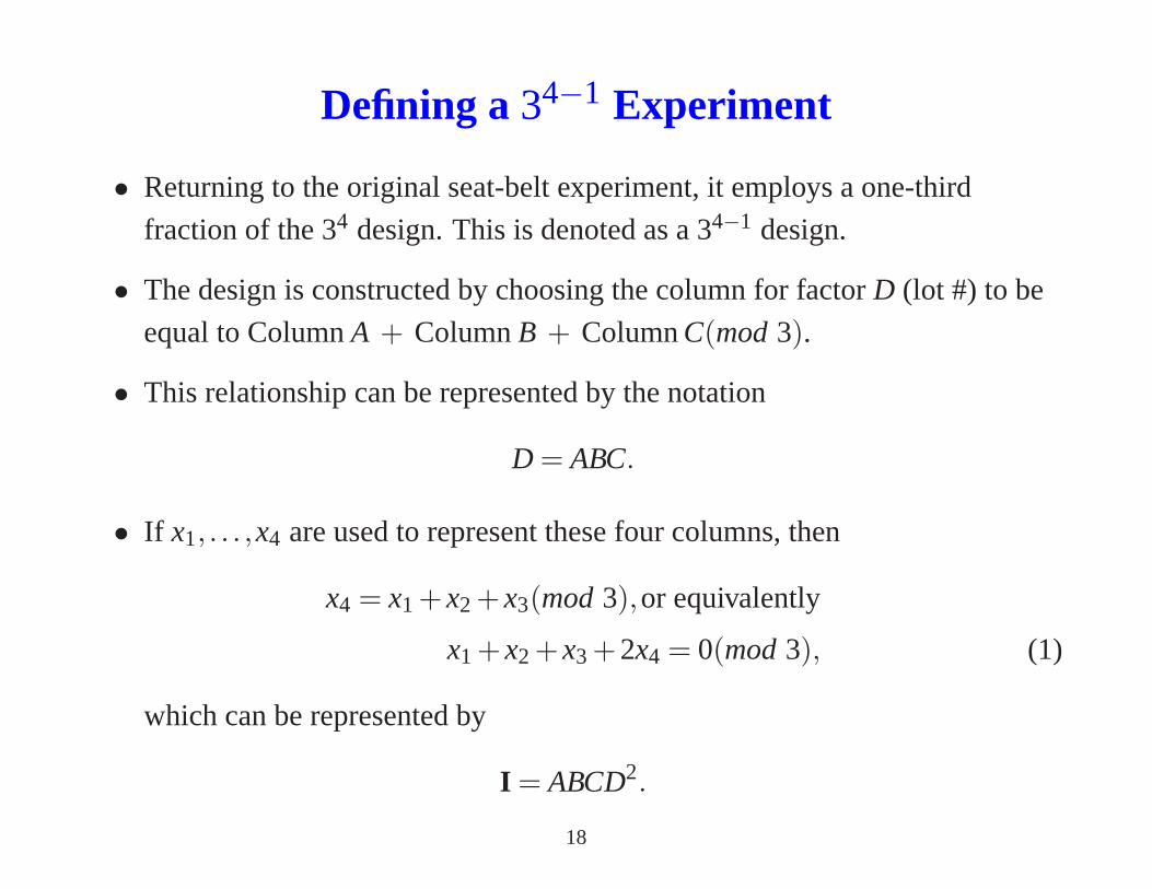
Defining a34−1 Experiment
• Returning to the original seat-belt experiment, it employsa one-third
fraction of the 34 design. This is denoted as a 34−1 design.
• The design is constructed by choosing the column for factorD (lot #) to be
equal to ColumnA + ColumnB + ColumnC(mod3).
• This relationship can be represented by the notation
D = ABC.
• If x1, . . . ,x4 are used to represent these four columns, then
x4 = x1 +x2 +x3(mod3),or equivalently
x1 +x2 +x3 +2x4 = 0(mod3), (1)
which can be represented by
I = ABCD2.
18
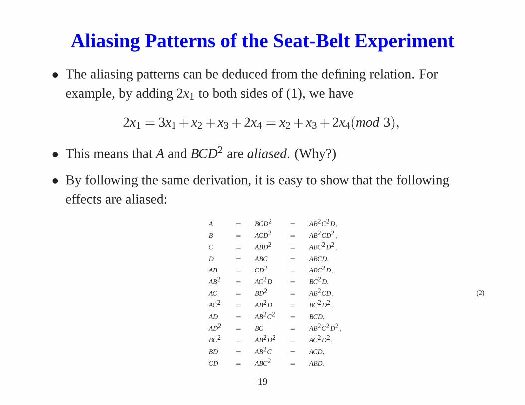
Aliasing Patterns of the Seat-Belt Experiment
• The aliasing patterns can be deduced from the defining relation. For
example, by adding 2x1 to both sides of (1), we have
2x1 = 3x1 +x2 +x3 +2x4 = x2 +x3 +2x4(mod3),
• This means thatA andBCD2 arealiased. (Why?)
• By following the same derivation, it is easy to show that the following
effects are aliased:
A = BCD2 = AB2C2D,
B = ACD2 = AB2CD2,
C = ABD2 = ABC2D2,
D = ABC = ABCD,
AB = CD2 = ABC2D,
AB2 = AC2D = BC2D,
AC = BD2 = AB2CD,
AC2 = AB2D = BC2D2,
AD = AB2C2 = BCD,
AD2 = BC = AB2C2D2,
BC2 = AB2D2 = AC2D2,
BD = AB2C = ACD,
CD = ABC2 = ABD.
(2)
19
Clear and Strongly Clear Effects
• If three-factor interactions are assumed negligible, fromthe aliasing relations in (2),
A, B, C, D, AB2, AC2, AD, BC2, BD andCD can be estimated.
• These main effects or components of two-factor interactions are calledclear because
they are not aliased with any other main effects or two-factor interaction
components.
• A two-factor interaction, sayA×B, is calledclear if both of its components,ABand
AB2, are clear.
• Note that each of the six two-factor interactions has only one component that is
clear; the other component is aliased with one component of another two-factor
interaction. For example, forA×B, AB2 is clear butAB is aliased withCD2.
• A main effect or two-factor interaction component is said tobestrongly clear if it is
not aliased with any other main effects, two-factor or three-factor interaction
components. A two-factor interaction is said to bestrongly clearif both of its
components are strongly clear.
20

A 35−2 Design
• 5 factors, 27 runs.
• The one-ninth fraction is defined byI = ABD2 = AB2CE2, from which two
additional relations can be obtained:
I = (ABD2)(AB2CE2) = A2CD2E2 = AC2DE
and
I = (ABD2)(AB2CE2)2 = B2C2D2E = BCDE2.
Therefore the defining contrast subgroup for this design consists of the
following defining relation:
I = ABD2 = AB2CE2 = AC2DE = BCDE2. (3)
21
Resolution and Minimum Aberration
• Let Ai be to denote the number of words of lengthi in the subgroup and
W = (A3,A4, . . .) to denote the wordlength pattern.
• Based onW, the definitions ofresolution andminimum aberration are the
same as given before in Section 5.2.
• The subgroup defined in (3) has four words, whose lengths are 3, 4, 4, and 4.
and henceW = (1,3,0). Another 35−2 design given byD = AB,E = AB2
has the defining contrast subgroup,
I = ABD2 = AB2E2 = ADE = BDE2,
with the wordlength patternW = (4,0,0). According to the aberration
criterion, the first design has less aberration than the second design.
• Moreover, it can be shown that the first design has minimum aberration.
22
General3k−p Design
• A 3k−p design is a fractional factorial design withk factors in 3k−p runs.
• It is a 3−pth fraction of the 3k design.
• The fractional plan is defined byp independent generators.
• How many factors can a 3k−p design study?
(3n−1)/2, wheren = k− p.
This design has 3n runs with the independent generatorsx1, x2, . . ., xn. We
can obtain altogether(3n−1)/2 orthogonal columns as different
combinations of∑ni=1 αixi with αi = 0, 1 or 2, where at least oneαi should
not be zero and the first nonzeroαi should be written as “1” to avoid
duplication.
• Forn=3, the(3n−1)/2 = 13 columns were given in Table 6.5 of WH book.
• A general algebraic treatment of 3k−p designs can be found in Kempthorne
(1952).23
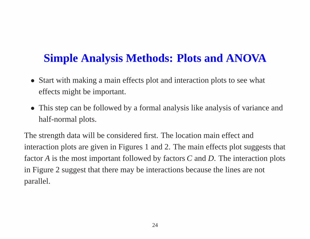
Simple Analysis Methods: Plots and ANOVA
• Start with making a main effects plot and interaction plots to see what
effects might be important.
• This step can be followed by a formal analysis like analysis of variance and
half-normal plots.
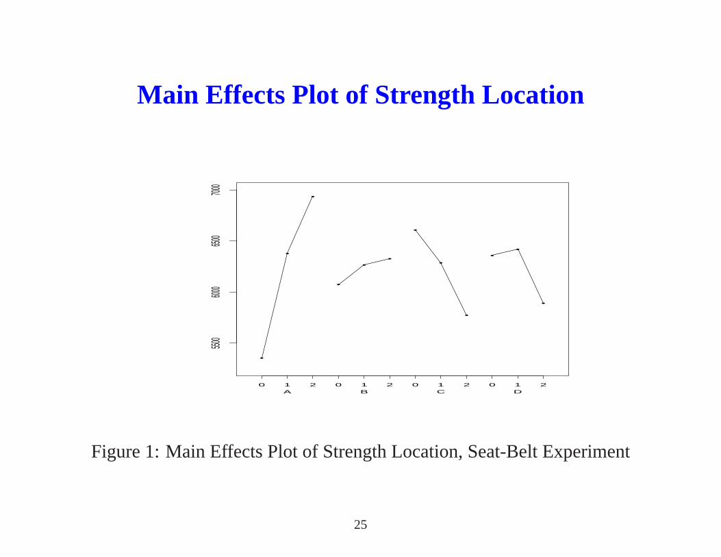
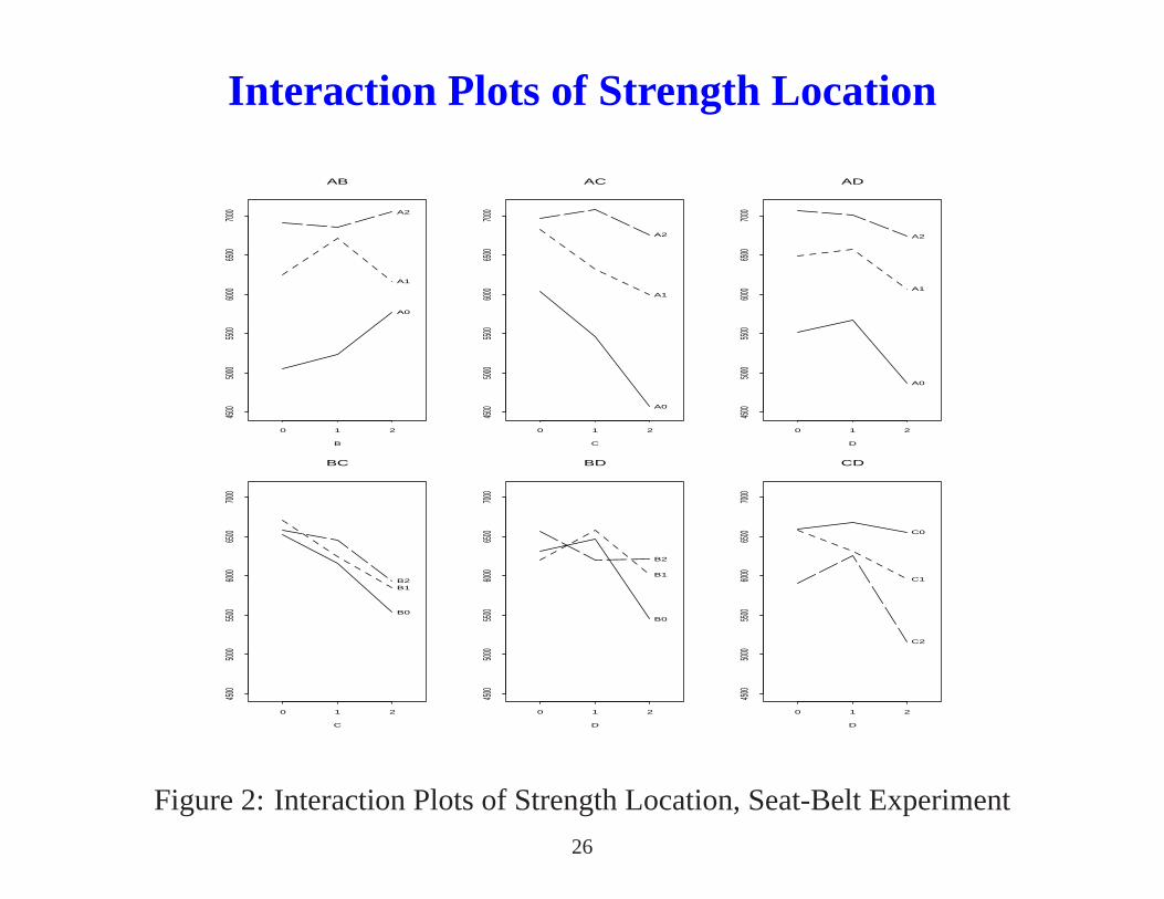
The strength data will be considered first. The location maineffect and
interaction plots are given in Figures 1 and 2. The main effects plot suggests that
factorA is the most important followed by factorsC andD. The interaction plots
in Figure 2 suggest that there may be interactions because the lines are not
parallel.
24
Main Effects Plot of Strength Location
•
•
•
•
••
•
•
•
••
•
5500
6000
6500
7000
0 1 2 0 1 2 0 1 2 0 1 2A B C D
Figure 1: Main Effects Plot of Strength Location, Seat-Belt Experiment
25
Interaction Plots of Strength Location
B
4500
5000
5500
6000
6500
7000
0 1 2
A0
A1
A2
AB
C
4500
5000
5500
6000
6500
7000
0 1 2
A0
A1
A2
AC
D
4500
5000
5500
6000
6500
7000
0 1 2
A0
A1
A2
AD
C
4500
5000
5500
6000
6500
7000
0 1 2
B0
B1B2
BC
D
4500
5000
5500
6000
6500
7000
0 1 2
B0
B1
B2
BD
D
4500
5000
5500
6000
6500
7000
0 1 2
C0
C1
C2
CD
Figure 2: Interaction Plots of Strength Location, Seat-Belt Experiment
26
ANOVA Table for Strength Location
Degrees of Sum of Mean
Source Freedom Squares Squares F p-value
A 2 34621746 17310873 85.58 0.000
B 2 938539 469270 2.32 0.108
AB= CD2 2 2727451 1363725 6.74 0.002
AB2 2 570795 285397 1.41 0.253
C 2 9549481 4774741 23.61 0.000
AC= BD2 2 2985591 1492796 7.38 0.001
AC2 2 886587 443294 2.19 0.122
BC= AD2 2 427214 213607 1.06 0.355
BC2 2 21134 10567 0.05 0.949
D 2 4492927 2246464 11.11 0.000
AD 2 263016 131508 0.65 0.526
BD 2 205537 102768 0.51 0.605
CD 2 245439 122720 0.61 0.549
residual 54 10922599 202270
27

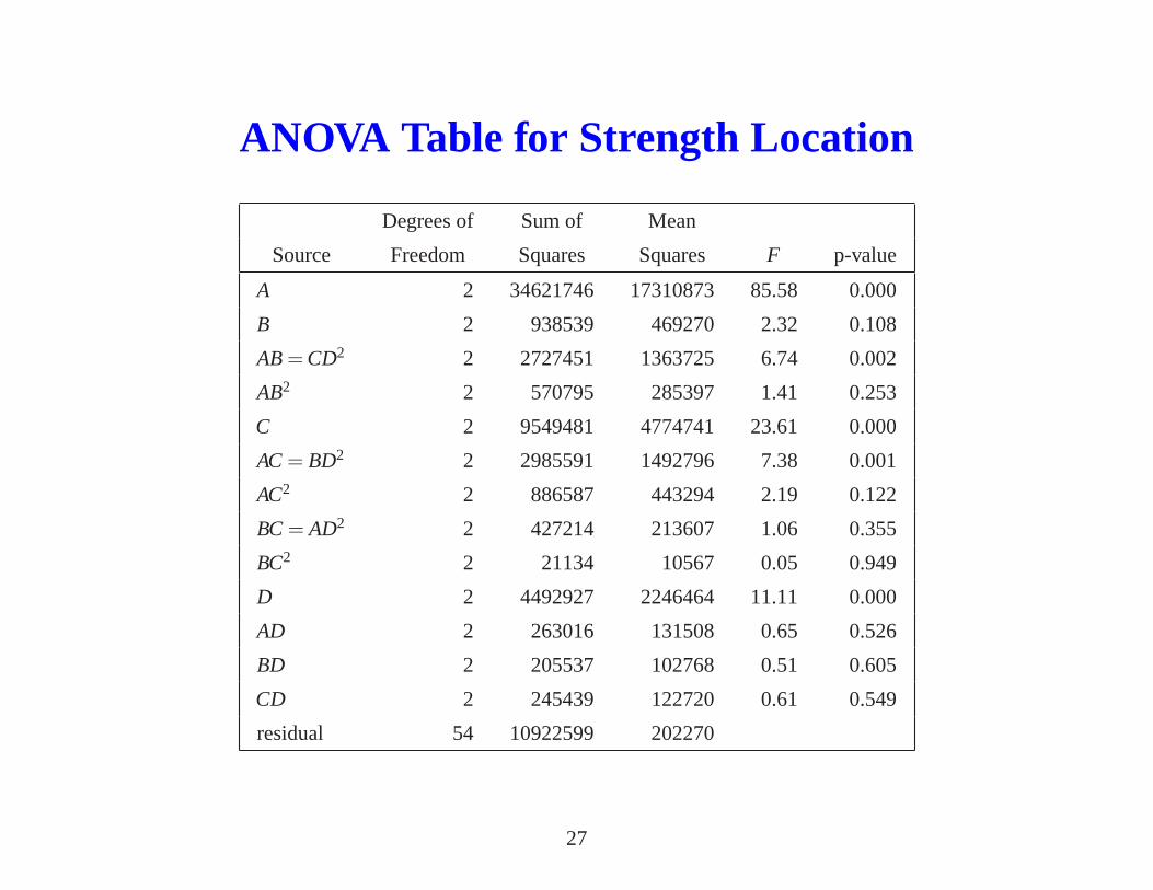
Analysis of Strength Location, Seat-Belt Experiment
• In equation (2), the 26 degrees of freedom in the experiment were grouped
into 13 sets of effects. The corresponding ANOVA table givesthe SS values
for these 13 effects.
• Based on the p values in the ANOVA Table, clearly the factorA, C andD
main effects are significant.
• Also two aliased sets of effects are significant,AB= CD2 andAC= BD2.
• These findings are consistent with those based on the main effects plot and
interaction plots. In particular, the significance ofABandCD2 is supported
by theA×B andC×D plots and the significance ofAC andBD2 by the
A×C andB×D plots.
28

Analysis of Strength Dispersion (i.e.,lns2) Data
The corresponding strength main effects plot and interaction plots are displayed
in Figures 3 and 4.
•
•
•
•
•
•
•
•
•
•
•
•
10.010.5
11.011.5
12.012.5
0 1 2 0 1 2 0 1 2 0 1 2A B C D
Figure 3: Main Effects Plot of Strength Dispersion, Seat-Belt Experiment
29

Interaction Plots of Strength Dispersion
B
89
1011
1213
0 1 2
A0
A1
A2
AB
C
89
1011
1213
0 1 2
A0
A1A2
AC
D
89
1011
1213
0 1 2
A0
A1
A2
AD
C
89
1011
1213
0 1 2
B0
B1
B2
BC
D
89
1011
1213
0 1 2
B0
B1
B2
BD
D
89
1011
1213
0 1 2
C0
C1
C2
CD
Figure 4: Interaction Plots of Strength Dispersion, Seat-Belt Experiment
30

Half-Normal Plots
• Since there is no replication for the dispersion analysis, ANOVA cannot be
used to test effect significance.
• Instead, a half-normal plot can be drawn as follows. The 26 df’s can be
divided into 13 groups, each having two df’s. These 13 groupscorrespond
to the 13 rows in the ANOVA table of page 27.
• The two degrees of freedom in each group can be decomposed further into a
linear effect and a quadratic effect with the contrast vectors 1√2(−1,0,1)
and 1√6(1,−2,1), respectively, where the values in the vectors are associated
with the lns2 values at the levels (0, 1, 2) for the group.
• Because the linear and quadratic effects are standardized and orthogonal to
each other, these 26 effect estimates can be plotted on the half-normal
probability scale as in Figure 5.
31
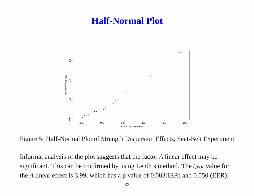
Half-Normal Plot
•• • • •
• • • • • • ••
• •• •
••
• • •
•
•
•
•
half-normal quantiles
abso
lute
con
stra
sts
0.0 0.5 1.0 1.5 2.0 2.5
0.0
0.5
1.0
1.5
.
Al
Figure 5: Half-Normal Plot of Strength Dispersion Effects,Seat-Belt Experiment
Informal analysis of the plot suggests that the factorA linear effect may be
significant. This can be confirmed by using Lenth’s method. The tPSE value for
theA linear effect is 3.99, which has a p value of 0.003(IER) and 0.050(EER).32
Analysis Summary
• A similar analysis can be performed to identify the flash location and
dispersion effects. See Section 6.5 of WH book.
• We can determine the optimal factor settings that maximize thestrength
locationby examining the main effects plot and interaction plots in
Figures 1 and 2 that correspond to the significant effects identified in the
ANOVA table.
• We can similarly determine the optimal factor settings thatminimize the
strength dispersion, the flash locationandflash dispersion, respectively.
• The most obvious findings: level 2 of factorA be chosen to maximize
strength while level 0 of factorA be chosen to minimize flash.
• There is an obvious conflict in meeting the two objectives. Trade-off
strategies for handling multiple characteristics and conflicting objectives
need to be considered (See Section 6.7 of WH).
33

An Alternative Analysis Method : Linear-Quadratic
System
In the seat-belt experiment, the factorsA,B andC are quantitative. The two
degrees of freedom in a quantitative factor, sayA, can be decomposed into the
linear and quadratic components.
Lettingy0, y1 andy2 represent the observations at level 0, 1 and 2, then thelinear
effectis defined as
y2−y0
and thequadratic effectas
(y2 +y0)−2y1,
which can be re-expressed as the difference between two consecutive linear
effects(y2−y1)− (y1−y0).
34
Linear and Quadratic Effects
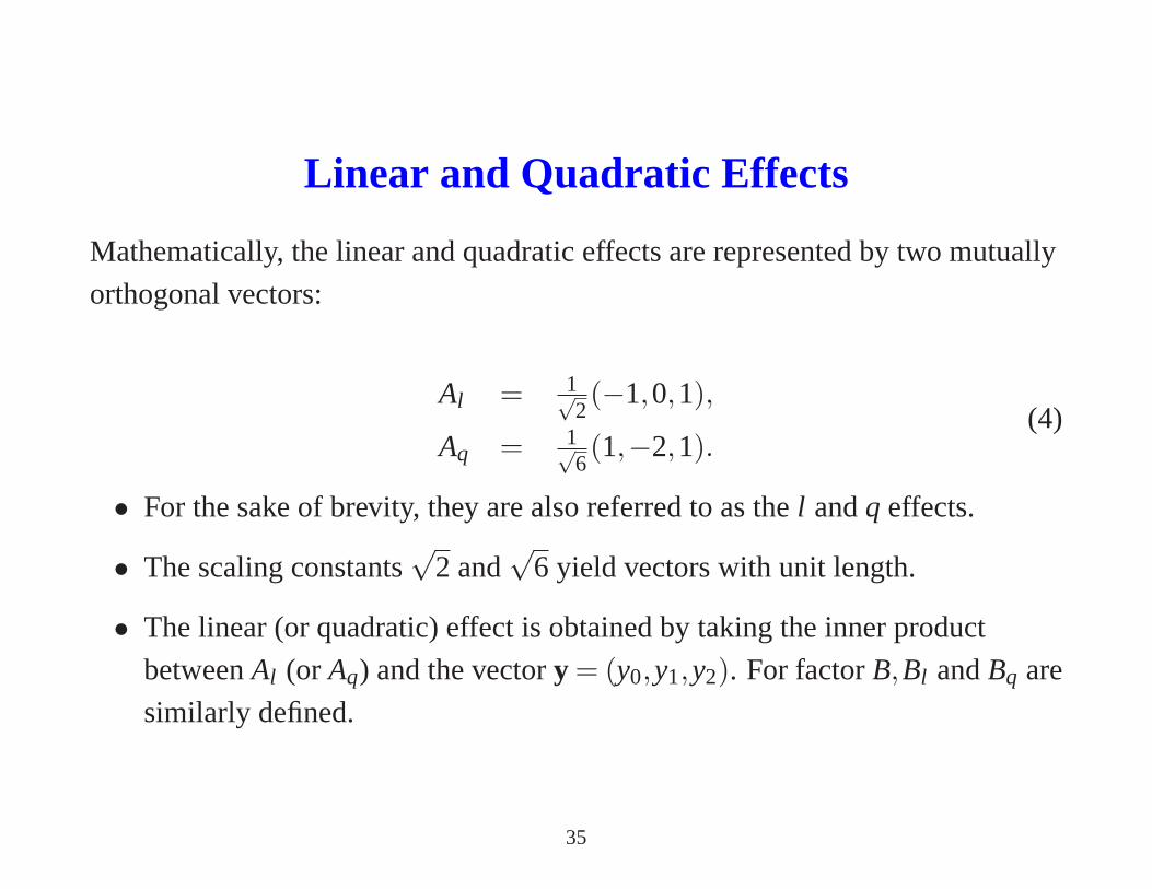
Mathematically, the linear and quadratic effects are represented by two mutually
orthogonal vectors:
Al = 1√2(−1,0,1),
Aq = 1√6(1,−2,1).
(4)
• For the sake of brevity, they are also referred to as thel andq effects.
• The scaling constants√
2 and√
6 yield vectors with unit length.
• The linear (or quadratic) effect is obtained by taking the inner product
betweenAl (or Aq) and the vectory = (y0,y1,y2). For factorB,Bl andBq are
similarly defined.
35
Linear and Quadratic Effects (contd)
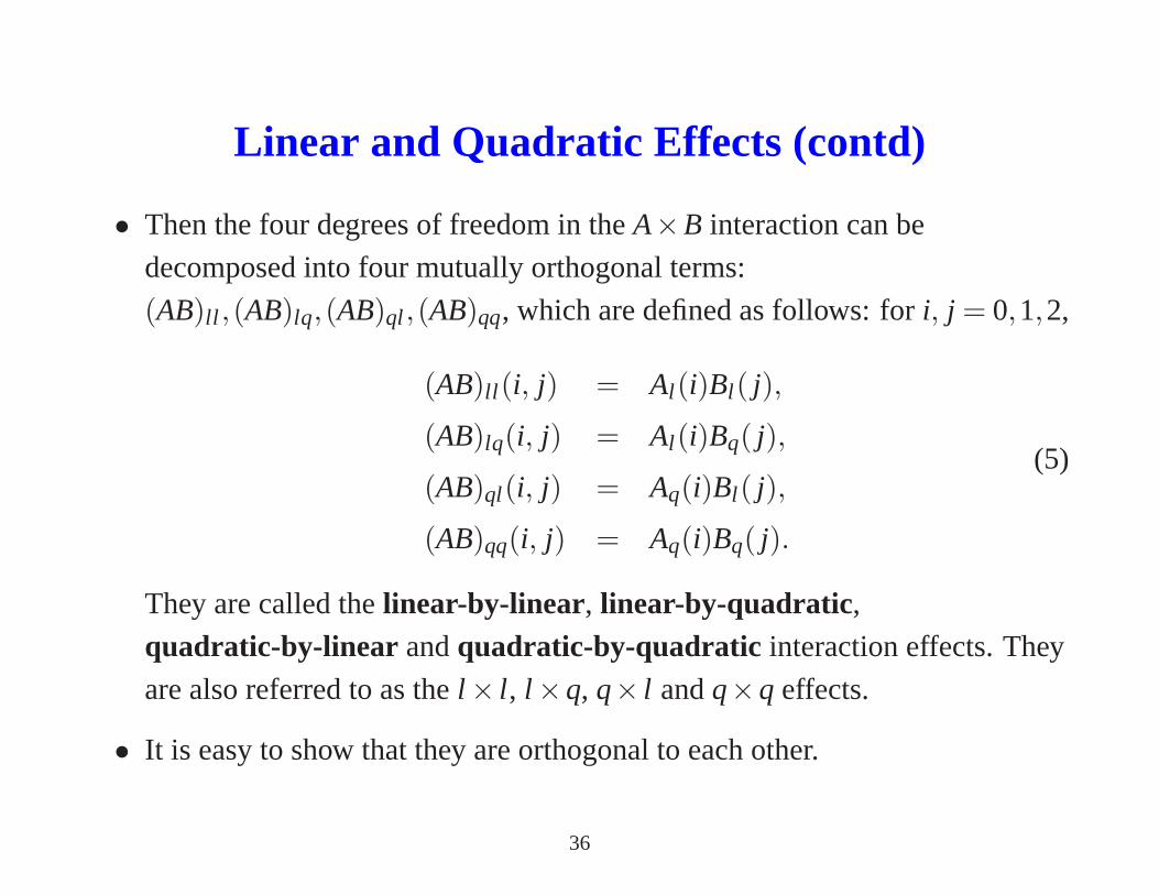
• Then the four degrees of freedom in theA×B interaction can be
decomposed into four mutually orthogonal terms:
(AB)ll ,(AB)lq,(AB)ql ,(AB)qq, which are defined as follows: fori, j = 0,1,2,
(AB)ll (i, j) = Al (i)Bl ( j),
(AB)lq(i, j) = Al (i)Bq( j),
(AB)ql(i, j) = Aq(i)Bl ( j),
(AB)qq(i, j) = Aq(i)Bq( j).
(5)
They are called thelinear-by-linear , linear-by-quadratic ,
quadratic-by-linear andquadratic-by-quadratic interaction effects. They
are also referred to as thel × l , l ×q, q× l andq×q effects.
• It is easy to show that they are orthogonal to each other.
36

Linear and Quadratic Effects (contd)
Using the nine level combinations of factorsA andB, y00, . . . ,y22 given in
Table 5, the contrasts(AB)ll , (AB)lq, (AB)ql , (AB)qq can be expressed as follows:
(AB)ll : 12{(y22−y20)− (y02−y00)},
(AB)lq: 12√
3{(y22+y20−2y21)− (y02+y00−2y01)},
(AB)ql : 12√
3{(y22+y02−2y12)− (y20+y00−2y10)},
(AB)qq: 16{(y22+y20−2y21)−2(y12+y10−2y11)+(y02+y00−2y01)}.
• An (AB)ll interaction effect measures the difference between the conditional
linearB effects at levels 0 and 2 of factorA.
• A significant(AB)ql interaction effect means that there is curvature in the
conditional linearB effect over the three levels of factorA.
• The other interaction effects(AB)lq and(AB)qq can be similarly interpreted.
37

Analysis of designs with resolution at leastV
• For designs of at least resolution V, all the main effects andtwo-factor
interactions are clear. Then, further decomposition of these effects
according to the linear-quadratic system allows all the effects (each with one
degree of freedom) to be compared in a half-normal plot.
• Note that for effects to be compared in a half-normal plot, they should be
uncorrelated and have the same variance.
38

Analysis of designs with resolution smaller thanV
• For designs with resolutionIII or IV , a more elaborate analysis method is
required to extract the maximum amount of information from the data.
• Consider the 33−1 design withC = ABwhose design matrix is given inTable 6.
Table 6: Design Matrix for the 33−1 DesignRun A B C
1 0 0 0
2 0 1 1
3 0 2 2
4 1 0 1
5 1 1 2
6 1 2 0
7 2 0 2
8 2 1 0
9 2 2 1
• Its main effects and two-factor interactions have the aliasing relations:
A = BC2,B = AC2,C = AB,AB2 = BC= AC. (6)
39
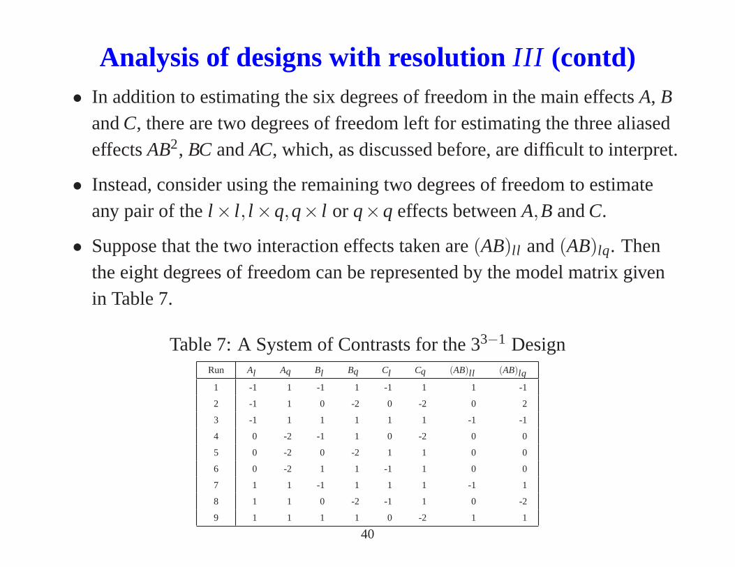
Analysis of designs with resolutionIII (contd)• In addition to estimating the six degrees of freedom in the main effectsA, B
andC, there are two degrees of freedom left for estimating the three aliasedeffectsAB2, BC andAC, which, as discussed before, are difficult to interpret.
• Instead, consider using the remaining two degrees of freedom to estimateany pair of thel × l , l ×q,q× l or q×q effects betweenA,B andC.
• Suppose that the two interaction effects taken are(AB)ll and(AB)lq. Thenthe eight degrees of freedom can be represented by the model matrix givenin Table 7.
Table 7: A System of Contrasts for the 33−1 DesignRun Al Aq Bl Bq Cl Cq (AB)ll (AB)lq
1 -1 1 -1 1 -1 1 1 -1
2 -1 1 0 -2 0 -2 0 2
3 -1 1 1 1 1 1 -1 -1
4 0 -2 -1 1 0 -2 0 0
5 0 -2 0 -2 1 1 0 0
6 0 -2 1 1 -1 1 0 0
7 1 1 -1 1 1 1 -1 1
8 1 1 0 -2 -1 1 0 -2
9 1 1 1 1 0 -2 1 1
40

Analysis of designs with resolutionIII (contd)• Because any component ofA×B is orthogonal toA and toB, there are only
four non-orthogonal pairs of columns whose correlations are:
Corr((AB)ll ,Cl ) = −√
38,
Corr((AB)ll ,Cq) = − 1√8,
Corr((AB)lq,Cl ) = 1√8,
Corr((AB)lq,Cq) = −√
38.
(7)
• Obviously,(AB)ll and(AB)lq can be estimated in addition to the three maineffects.
• Because the last four columns are not mutually orthogonal, they cannot beestimated with full efficiency.
• The estimability of(AB)ll and(AB)lq demonstrates an advantage of thelinear-quadratic system over the orthogonal components system. For thesame design, theAB interaction component cannot be estimated because it isaliased with the main effectC.
41

Analysis Strategy for Qualitative Factors
• For a qualitative factor like factorD (lot number) in the seat-belt
experiment, the linear contrast(−1,0,+1) may make sense because it
represents the comparison between levels 0 and 2.
• On the other hand, the “quadratic” contrast(+1,−2,+1), which compares
level 1 with the average of levels 0 and 2, makes sense only if such a
comparison is of practical interest. For example, if levels0 and 2 represent
two internal suppliers, then the “quadratic” contrast measures the difference
between internal and external suppliers.
42
Analysis Strategy for Qualitative Factors (contd)
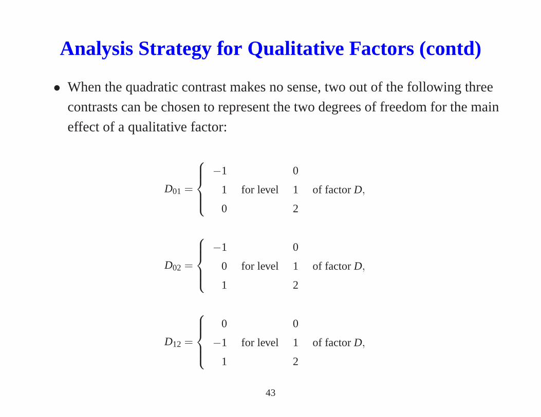
• When the quadratic contrast makes no sense, two out of the following three
contrasts can be chosen to represent the two degrees of freedom for the main
effect of a qualitative factor:
D01 =
−1 0
1 for level 1 of factorD,
0 2
D02 =
−1 0
0 for level 1 of factorD,
1 2
D12 =
0 0
−1 for level 1 of factorD,
1 2
43
Analysis Strategy for Qualitative Factors (contd)
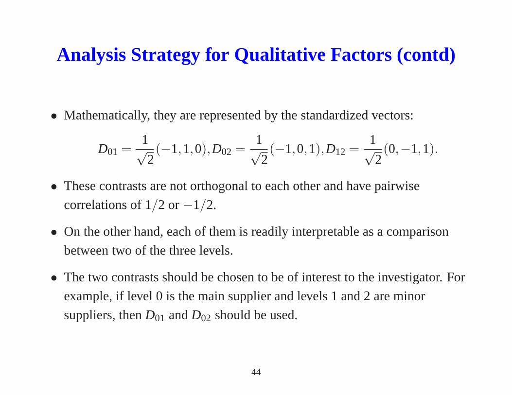
• Mathematically, they are represented by the standardized vectors:
D01 =1√2(−1,1,0),D02 =
1√2(−1,0,1),D12 =
1√2(0,−1,1).
• These contrasts are not orthogonal to each other and have pairwise
correlations of 1/2 or−1/2.
• On the other hand, each of them is readily interpretable as a comparison
between two of the three levels.
• The two contrasts should be chosen to be of interest to the investigator. For
example, if level 0 is the main supplier and levels 1 and 2 are minor
suppliers, thenD01 andD02 should be used.
44
Qualitative and Quantitative Factors
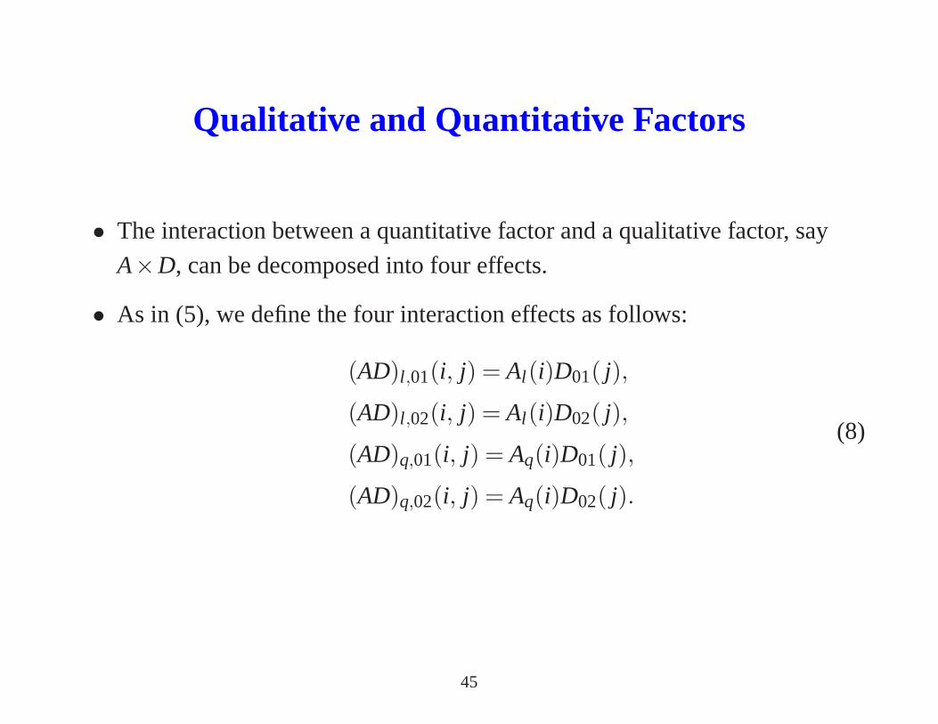
• The interaction between a quantitative factor and a qualitative factor, say
A×D, can be decomposed into four effects.
• As in (5), we define the four interaction effects as follows:
(AD)l ,01(i, j) = Al (i)D01( j),
(AD)l ,02(i, j) = Al (i)D02( j),
(AD)q,01(i, j) = Aq(i)D01( j),
(AD)q,02(i, j) = Aq(i)D02( j).
(8)
45

Variable Selection Strategy
Since many of these contrasts are not mutually orthogonal, ageneral purpose
analysis strategy cannot be based on the orthogonality assumption. Therefore,
the following variable selection strategy is recommended.
(i) For a quantitative factor, sayA, useAl andAq for theA main effect.
(ii) For a qualitative factor, sayD, useDl andDq if Dq is interpretable; otherwise, select two
contrasts fromD01,D02, andD12 for theD main effect.
(iii) For a pair of factors, sayX andY, use the products of the two contrasts ofX and the two
contrasts ofY (chosen in (i) or (ii)) as defined in (5) or (8) to represent thefour degrees of
freedom in the interactionX×Y.
(iv) Using the contrasts defined in (i)-(iii) for all the factors and their two-factor interactions as
candidate variables, perform a stepwise regression or subset selection procedure to identify a
suitable model. To avoid incompatible models, use the effect heredity principle to rule out
interactions whose parent factors are both not significant.
(v) If all the factors are quantitative, use the original scale,sayxA, to represent the linear effect ofA,
x2A the quadratic effect andxi
Ax jB the interaction betweenxi
A andx jB. This works particularly well
if some factors have unevenly spaced levels.
46

Analysis of Seat-Belt Experiment
• Returning to the seat-belt experiment, although the original design has
resolution IV, its capacity for estimating two-factor interactions is much
better than what the definition of resolution IV would suggest.
• After estimating the four main effects, there are still 18 degrees of freedom
available for estimating some components of the two-factorinteractions.
• From (2),A, B, C andD are estimable and only one of the two components
in each of the six interactionsA×B, A×C, A×D, B×C, B×D andC×D
is estimable.
• Because of the difficulty of providing a physical interpretation of an
interaction component, a simple and efficient modeling strategy that does
not throw away the information in the interactions is to consider the
contrasts(Al ,Aq), (Bl ,Bq), (Cl ,Cq) and(D01,D02,D12) for the main effects
and the 30 products between these four groups of contrasts for the
interactions.
47

Analysis of Seat-Belt Experiment (contd)
• Using these 39 contrasts as the candidate variables, the variable selection
procedure was applied to the data.
• Performing a stepwise regression on the strength data (responsey1), the
following model with anR2 of 0.811 was identified:
y1 = 6223.0741+1116.2859Al −190.2437Aq +178.6885Bl
−589.5437Cl +294.2883(AB)ql +627.9444(AC)ll
−191.2855D01−468.4190D12−486.4444(CD)l ,12
(9)
• Note that this model obeys effect heredity. TheA, B, C andD main effects
andA×B, A×C andC×D interactions are significant. In contrast, the
simple analysis from the previous section identified theA, C andD main
effects and theAC(= BD2) andAB(= CD2) interaction components as
significant.
48

Analysis of Seat-Belt Experiment (contd)
• Performing a stepwise regression on the flash data (responsey2), the
following model with anR2 of 0.857 was identified:
y2 = 13.6657+1.2408Al +0.1857Bl
−0.8551Cl +0.2043Cq−0.9406(AC)ll
−0.3775(AC)ql −0.3765(BC)qq−0.2978(CD)l ,12
(10)
• Again, the identified model obeys effect heredity. TheA, B, andC main
effects andA×C, B×C andC×D interactions are significant. In contrast,
the simple analysis from the previous section identified theA andC main
effects and theAC(= BD2), AC2 andBC2 interaction components as
significant.
49

Comments on Board
50