unit 4 uncertain knowledge complete

7/27/2019 Unit 4 Uncertain Knowledge Complete

http://slidepdf.com/reader/full/unit-4-uncertain-knowledge-complete 1/14

Prepared by,

Abdurrahman

Asst.Professor-CSE Dept-JCE

UNIT-VI

UNCERTAIN KNOWLEDGE AND REASONING

When an agent almost never has access to the whole truth about their environment then the

agents must, therefore, act under uncertainty.

Handling uncertain knowledge

Possible Question: 8 Marks

Explain how you will handle uncertain knowledge.

Explain Probabilistic reasoning.

• Diagnosis-whether for medicine, automobile repair, or whatever-is a task that almost

always involves uncertainty.

• If we try to write rules for dental diagnosis using first-order logic,

• Not all patients with toothaches have cavities; some of them have gum disease, an

abscess, or one of several other problems.

• Domain like medical diagnosis fails for three main reasons

o Laziness

o Theoretical ignorance

o Practical ignorance

• The agent's knowledge can only be a degree of belief in the relevant sentences.

• The main tool for dealing with degrees of belief will be probability theory, which

assigns to each sentence a numerical degree of belief between 0 and 1.

• Probability provides a way of summarizing the uncertainty that comes from lazinessand ignorance.

• Assigning a probability of 0 to a given sentence corresponds to an unequal belief that

the sentence is false.

• While assigning a probability of 1 corresponds to an unequivocal belief that the

sentence is true.

• Probabilities between 0 and 1 correspond to intermediate degrees of belief in the truth

of the sentence.

• In probability theory, a sentence such as "The probability that the patient has a cavity

is 0.8" is about the agent's beliefs, not directly about the world.

• All probability statements must therefore indicate the evidence with respect to whichthe probability is being assessed.

Basic Probability Notation

8Marks: What are basic probabilities Notation?

Propositions:

• Probability theory typically uses a language that is slightly more expressive than

propositional logic.

• The basic element of the language is the random variable, which can be thought of asreferring to a "part" of the world whose "status" is initially unknown.



Prepared by,

Abdurrahman


• We use lowercase, single-letter names to represent an unknown random variable, for

example

• Each random variable has a domain of values that it can take on.

• For example, the domain of Cavity might be (true, false).

• Random variables are typically divided into three kinds, depending on the type of the

domain:

1. Boolean random variables,

2. Discrete random variables,

3. Continuous random variables

Atomic events:

• An atomic event is a complete specification of the state of the world about which the

agent is uncertain.

• It can be thought of as an assignment of particular values to all the variables of whichthe world is composed.

• For example, if my world consists of only the Boolean variables Cavity and

Toothache, then there are just four distinct atomic events; the proposition Cavity

=false And Toothache = true js one such event.

Prior probability:

• The unconditional or prior probability associated with a proposition a is the degree

of belief accorded to it in the absence of any other information; it is written as P(a).

•

F or example, if the prior probability that I have a cavity is 0.1, then we would write P(Cavity = true) = 0.1 or P(cavity) = 0.1 .

Conditional probability:

• Once the agent has obtained some evidence concerning the previously unknown

random variables making up the domain, prior probabilities are no longer applicable.

• Instead, a conditional or posterior probability is used.

• The notation used is P (alb), where a and b are any proposition.

• This is read as "the probability of a, given that all we know is b."

• For example, P(cavity1 toothache) = 0.8 indicates that if a patient is observed to have

a toothache and no other information is yet available, then the probability of the

patient's having a cavity will be 0.8.

BAYES R U L E 2Marks:

• The product rule can be written in two forms because of the commutativity of conjunction:

• Equating the two right-hand sides and dividing by P(a), we get



Prepared by,

Abdurrahman


• This equation is known as Bayes' rule (also Bayes' law or Bayes' theorem).

BAYESIAN NETWORK

8 or 16 Marks: Explain in detail about representing knowledge in uncertain domain.

Definition:

• A Bayesian network is a data structure to represent the dependencies among

variables and to give a concise specification of any full joint probability distribution.

• A Bayesian network is a directed graph in which each node is annotated with

quantitative probability information.

Specification of Bayesian Network

1. A set of random variables makes up the nodes of the network. Variables may be

discrete or continuous.

2. A set of directed links or arrows connects pairs of nodes. If there is an arrow from

node X to node Y, X is said to be a parent of Y.

3. Each node Xi, has a conditional probability distribution P(Xi,|Parents(Xi,)) that

quantifies the effect of the parents on the node.

4. The graph has no directed cycles (and hence is a directed, acyclic graph, or DAG).

• Once the topology of the Bayesian network is laid out, we need only specify a

conditional probability distribution for each variable, given its parents.

• Consider the following example,

a new burglar alarm installed at home. It is fairly reliable at detecting a burglary,

but also responds on occasion to minor earthquakes. (This example is due to Judea

Pearl, a resident of Los Angeles-hence the acute interest in earthquakes.) You also

have two neighbours, John and Mary, who have promised to call you at work when

they hear the alarm. John always calls when he hears the alarm, but sometimes

confuses the telephone ringing with the alarm and calls then, too. Mary, on the

other hand, likes rather loud music and sometimes misses the alarm altogether.

•

Given the evidence of who has or has not called, we would like to estimate the probability of a burglary. The Bayesian network for this is given below:



Prepared by,

Abdurrahman


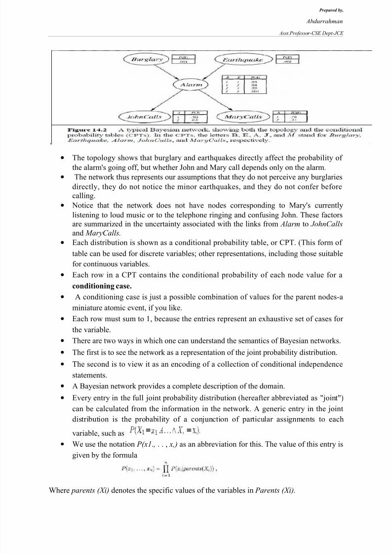
• The topology shows that burglary and earthquakes directly affect the probability of

the alarm's going off, but whether John and Mary call depends only on the alarm.

• The network thus represents our assumptions that they do not perceive any burglaries

directly, they do not notice the minor earthquakes, and they do not confer before

calling.• Notice that the network does not have nodes corresponding to Mary's currently

listening to loud music or to the telephone ringing and confusing John. These factors

are summarized in the uncertainty associated with the links from Alarm to JohnCalls

and MaryCalls.

• Each distribution is shown as a conditional probability table, or CPT. (This form of

table can be used for discrete variables; other representations, including those suitable

for continuous variables.

• Each row in a CPT contains the conditional probability of each node value for a

conditioning case.

• A conditioning case is just a possible combination of values for the parent nodes-a

miniature atomic event, if you like.

• Each row must sum to 1, because the entries represent an exhaustive set of cases for

the variable.

• There are two ways in which one can understand the semantics of Bayesian networks.

• The first is to see the network as a representation of the joint probability distribution.

• The second is to view it as an encoding of a collection of conditional independence

statements.

•A Bayesian network provides a complete description of the domain.

• Every entry in the full joint probability distribution (hereafter abbreviated as "joint")

can be calculated from the information in the network. A generic entry in the joint

distribution is the probability of a conjunction of particular assignments to each

variable, such as

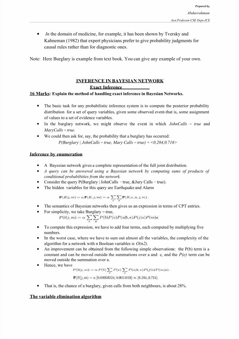
• We use the notation P(x1. , . . , x,) as an abbreviation for this. The value of this entry is

given by the formula

Where parents (Xi) denotes the specific values of the variables in Parents (Xi).



Prepared by,

Abdurrahman


• Thus, each entry in the joint distribution is represented by the product of the

appropriate elements of the Conditional probability tables (CPTs) in the Bayesian

network.

• The CPTs therefore provide a decomposed representation of the joint distribution.

•

To illustrate this, we can calculate the probability that the alarm has sounded, butneither a burglary nor an earthquake has occurred, and both John and Mary call. We

use single-letter names for the variables:

A method for constructing Bayesian networks

• The above equation defines what a given Bayesian network means. First, we rewrite

the joint distribution in terms of a conditional probability, using the product rule.

• Then we repeat the process, reducing each conjunctive probability to a conditional

probability and a smaller conjunction. We end up with one big product:

• This identity holds true for any set of random variables and is called the chain rule.• By Comparing the specification of the joint distribution is equivalent to the general

assertion that, for every variable Xi in the network,

Provided that

• This last condition is satisfied by labelling the nodes in any order that is consistent

with the partial order implicit in the graph structure.

Compactness and node ordering

• There are domains in which each variable can be influenced directly by all the others,

so that the network is fully connected.

• Then specifying the conditional probability tables requires the same amount of

information as specifying the joint distribution.

• In some domains, there will be slight dependencies that should strictly be included by

adding a new link.

• Consider the burglary example again.



Prepared by,

Abdurrahman


• Suppose we decide to add the nodes in the order MaryCalls, JohnCalls, Alarm,

Burglary, Earth quake. Then we get the somewhat more complicated network shown

in Figure below.

• The process goes as follows:

o Adding Mary Calls: No parents.

o Adding JohnCalls: If Mary calls, that probably means the alarm has gone off,

which of course would make it more likely that John calls. Therefore,

JohnCalls needs Mary Calls as a parent

o Adding Alarm: Clearly, if both call, it is more likely that the alarm has gone

off than if just one or neither calls, so we need both MaryCalls and JohnCalls

as parents.

o Adding Burglary: If we know the alarm state, then the call from John or

Mary might give us information about our phone ringing or Mary's music, but

not about burglary:

Hence we need just Alarm as parent.

o Adding Earthquake: if the alarm is on, it is more likely that there has been an

earthquake. (The alarm is an earthquake detector of sorts.)

• But if we know that there has been a burglary, then that explains the alarm, and the

probability of an earthquake would be only slightly above normal. Hence, we need

both Alarm and Burglary as parents.

• If we stick to a causal model, we end up having to specify fewer numbers, and the

numbers will often be easier to come up with.



Prepared by,

Abdurrahman


• In the domain of medicine, for example, it has been shown by Tversky and

Kahneman (1982) that expert physicians prefer to give probability judgments for

causal rules rather than for diagnostic ones.

Note: Here Burglary is example from text book. You can give any example of your own.

INFERENCE IN BAYESIAN NETWORK

Exact Inference

16 Marks: Explain the method of handling exact inference in Bayesian Networks.

• The basic task for any probabilistic inference system is to compute the posterior probability

distribution for a set of query variables, given some observed event-that is, some assignment

of values to a set of evidence variables.• In the burglary network, we might observe the event in which JohnCalls = true and

MaryCalls = true.

• We could then ask for, say, the probability that a burglary has occurred:

P(Burglary | JohnCalls = true, Mary Calls = true) = <0.284,0.716>

Inference by enumeration

• A Bayesian network gives a complete representation of the full joint distribution.

• A query can be answered using a Bayesian network by computing sums of products of

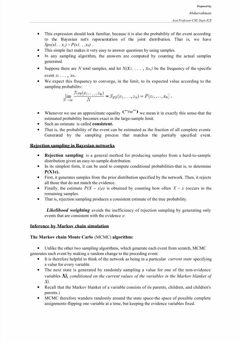
conditional probabibities from the network.• Consider the query P(Burglary | JohnCalls = true, &Jury Calls = true).

• The hidden variables for this query are Earthquake and Alarm

• The semantics of Bayesian networks then gives us an expression in terms of CPT entries.

• For simplicity, we take Burglary = true,

• To compute this expression, we have to add four terms, each computed by multiplying five

numbers.

• In the worst case, where we have to sum out almost all the variables, the complexity of thealgorithm for a network with n Boolean variables is O(n2).

• An improvement can be obtained from the following simple observations: the P(b) term is a

constant and can be moved outside the summations over a and e, and the P(e) term can be

moved outside the summation over a.

• Hence, we have

• That is, the chance of a burglary, given calls from both neighbours, is about 28%.

The variable elimination algorithm



Prepared by,

Abdurrahman


• The enumeration algorithm can be improved substantially by eliminating repeated

calculations do the calculation once and save the results for later use. This is a form of

dynamic programming.

• The Variable elimination works by evaluating expressions such in right-to-left order.

•Intermediate results are stored, and summations over each variable are done only for those

portions of the expression that depend on the variable.

• Let us illustrate this process for the burglary network. We evaluate the expression

• Each part of the expression is annotated with the name of the associated variable, these parts

are called factors.

• The steps are as follows,

1. The factor for M, P (m|a), does not require summing over M (because M's value is already

fixed), the probability is stored, given each value of a, in a two-element vector,as

(The f M means that M was used to produce f.)

2. The factor for J is stored as the two-element vector fj(A).

3. The factor for A is P (alB, e), which will be a 2 x 2 x 2 matrix f A(A, B, E).

Clustering algorithms

• If we want to compute posterior probabilities for all the variables in a network, however, it

can be less efficient.

• For example, in a polytree network, one would need to issue O(n) queries costing O(n) each,for a total of O(n^2) time.

• Using clustering algorithms (also known as Join tree algorithms), the time can be reduced to

O(n).

• For this reason, these algorithms are widely used in commercial Bayesian network tools.

• The basic idea of clustering is to join individual nodes of the network to form cluster nodes in

such a way that the resulting network is a polytree.

• Once the network is in polytree form, a special-purpose inference algorithm is applied.

• This algorithm is able to compute posterior probabilities for all the non-evidence nodes in the

network in time O(n), where n is now the size of the modified network.



Prepared by,

Abdurrahman


Approximate inference

16 Marks: Explain the method of handling approximate inference in Bayesian Networks.

•Monte Carlo algorithms, that provide approximate answers whose accuracy depends on thenumber of samples generated.

• Monte Carlo algorithms have become widely used in computer science to estimate quantities

that are difficult to calculate exactly.

• There are two families of algorithms: direct sampling and Markov chain sampling.

Direct sampling methods

• The primitive element in any sampling algorithm is the generation of samples from a known

Probability distribution.

• For example, an unbiased coin can be thought of as a random variable Coin with values

(heads, tails) and a prior distribution P(Coin) = (0.5,0.5).

• Sampling from this distribution is exactly like flipping the coin: with probability 0.5 it will

return heads, and with probability 0.5 it will return tails.

• The simplest kind of random sampling process for Bayesian networks generates events from a

network that has no evidence associated with it.

• The idea is to sample each variable in turn, in topological order.

• The probability distribution from which the value is sampled is conditioned on the values

already assigned to the variable's parents.

• We can illustrate its operation on the Rain Sprinkler network assuming an ordering

[Cloudy,Sprinkler, Rain, WetGrass]:

1. Sample from P (C1oudy) = (0.5, 0.5); suppose this returns true.2. Sample from P ( Sprinkler | Cloudy = true) = (0.:L , 0.9);suppose this returns false.

3. Sample from P (Rain|cloudy = true) = (0.8,0.2);suppose this returns true.

4. Sample from P ( WetGrass(Sprink1er = false, Rain = true) = (0.9,O.l);suppose this returns true.

• In this case, PRIOR -SAMPLE returns the event [true,f alse, true, true].

• First, let S pS( x1 , . . . , xn) be the probability that a specific event is generated by the PRIOR -

SAMPLE algorithm. The sampling process,

we have because each sampling step depends only on the parent values.



Prepared by,

Abdurrahman


• This expression should look familiar, because it is also the probability of the event according

to the Bayesian net's representation of the joint distribution. That is, we have

Sps(xl.. . x,) = P(x1. . .xn ) .

• This simple fact makes it very easy to answer questions by using samples.

• In any sampling algorithm, the answers are computed by counting the actual samples

generated.

• Suppose there are N total samples, and let N( x1 , . . . , xn ,) be the frequency of the specific

event XI, . . . , xn ,.

• We expect this frequency to converge, in the limit, to its expected value according to the

sampling probability:

• Whenever we use an approximate equality we mean it in exactly this sense-that the

estimated probability becomes exact in the large-sample limit.• Such an estimate is called consistent.

• That is, the probability of the event can be estimated as the fraction of all complete events

Generated by the sampling process that matches the partially specified event.

Rejection sampling in Bayesian networks

• Rejection sampling is a general method for producing samples from a hard-to-sample

distribution given an easy-to-sample distribution.

• In its simplest form, it can be used to compute conditional probabilities-that is, to determine

P(X1e).

•

First, it generates samples from the prior distribution specified by the network. Then, it rejectsall those that do not match the evidence.

• Finally, the estimate P(X = x|e) is obtained by counting how often X = x (occurs in the

remaining samples.

• That is, rejection sampling produces a consistent estimate of the true probability.

Likelihood weighting avoids the inefficiency of rejection sampling by generating only

events that are consistent with the evidence e.

Inference by Markov chain simulation

The Markov chain Monte Carlo (MCMC) algorithm:

• Unlike the other two sampling algorithms, which generate each event from scratch, MCMC

generates each event by making a random change to the preceding event.

• It is therefore helpful to think of the network as being in a particular current state specifying

a value for every variable.

• The next state is generated by randomly sampling a value for one of the non-evidence

variables Xi, conditioned on the current values of the variables in the Markov blanket of

Xi.

• Recall that the Markov blanket of a variable consists of its parents, children, and children's

parents.)

•MCMC therefore wanders randomly around the state space-the space of possible completeassignments-flipping one variable at a time, but keeping the evidence variables fixed.



Prepared by,

Abdurrahman


Working Of MCMC:

• The sampling process settles into a "dynamic equilibrium" in which the long-run fraction

of time spent in each state is exactly proportional to its posterior probability.

• This remarkable property follows from the specific transition probability with which the

process moves from one state to another, as defined by the conditional distribution given the

Markov blanket of the variable being sampled.

• MCMC is a powerful method for computing with probability models and many variants have

been developed, including the simulated annealing algorithm.

TEMPORAL MODEL

8Marks: Discuss about Temporal Model

• A temporal probability model can be thought of as containing a transition model describing

the evolution and a sensor model describing the observation process.

• The potentially infinite number of parents, is solved by making what is called a Markov

assumption- that is, that the current state depends on only a finite history of previous states.

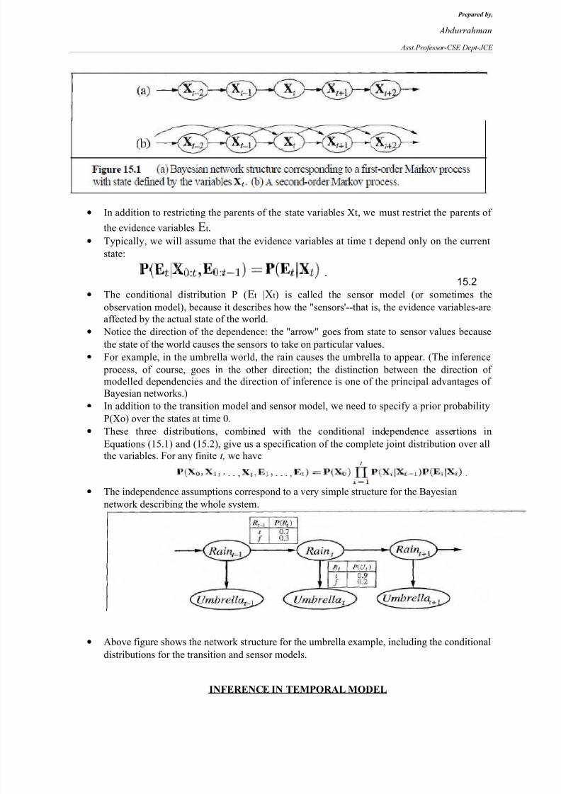
• The simplest is the first-order Markov process, in which the current state depends only on the

previous state and not on any earlier states.

• In a first-order Markov process, the laws describing how the state evolves over time are

contained entirely within the conditional distribution P(Xt |Xt-l), which is the transition

model for first-order processes.

• The transition model for a second-order Markov process is the conditional distribution

P(Xt | Xt-2, Xt-l)



Prepared by,

Abdurrahman


• In addition to restricting the parents of the state variables Xt, we must restrict the parents of

the evidence variables Et.

• Typically, we will assume that the evidence variables at time t depend only on the current

state:

15.2

• The conditional distribution P (Et |Xt) is called the sensor model (or sometimes the

observation model), because it describes how the "sensors'--that is, the evidence variables-are

affected by the actual state of the world.

• Notice the direction of the dependence: the "arrow" goes from state to sensor values because

the state of the world causes the sensors to take on particular values.

• For example, in the umbrella world, the rain causes the umbrella to appear. (The inference

process, of course, goes in the other direction; the distinction between the direction of

modelled dependencies and the direction of inference is one of the principal advantages of

Bayesian networks.)

• In addition to the transition model and sensor model, we need to specify a prior probability

P(Xo) over the states at time 0.• These three distributions, combined with the conditional independence assertions in

Equations (15.1) and (15.2), give us a specification of the complete joint distribution over all

the variables. For any finite t, we have

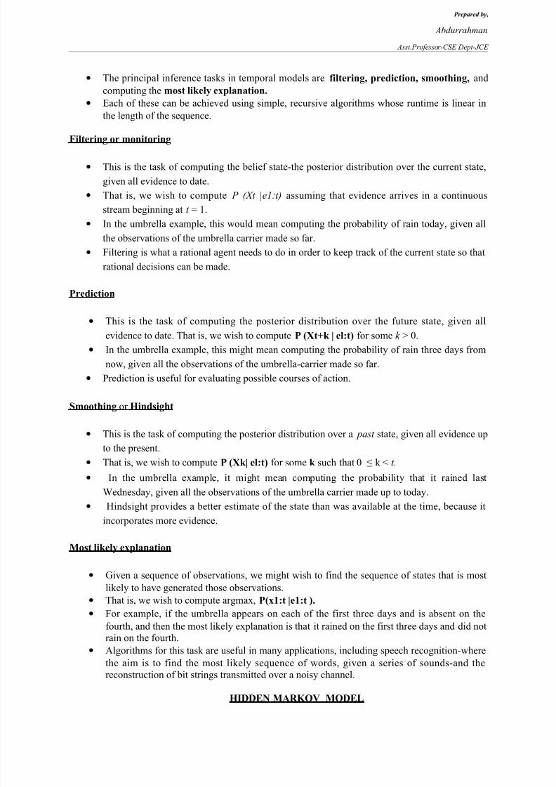
• The independence assumptions correspond to a very simple structure for the Bayesian

network describing the whole system.

• Above figure shows the network structure for the umbrella example, including the conditional

distributions for the transition and sensor models.

INFERENCE IN TEMPORAL MODEL



Prepared by,

Abdurrahman


• The principal inference tasks in temporal models are filtering, prediction, smoothing, and

computing the most likely explanation.

• Each of these can be achieved using simple, recursive algorithms whose runtime is linear in

the length of the sequence.

Filtering or monitoring

• This is the task of computing the belief state-the posterior distribution over the current state,

given all evidence to date.

• That is, we wish to compute P (Xt |e1:t) assuming that evidence arrives in a continuous

stream beginning at t = 1.

• In the umbrella example, this would mean computing the probability of rain today, given all

the observations of the umbrella carrier made so far.

• Filtering is what a rational agent needs to do in order to keep track of the current state so that

rational decisions can be made.

Prediction

• This is the task of computing the posterior distribution over the future state, given all

evidence to date. That is, we wish to compute P (Xt+k | el:t) for some k > 0.

• In the umbrella example, this might mean computing the probability of rain three days from

now, given all the observations of the umbrella-carrier made so far.

• Prediction is useful for evaluating possible courses of action.

Smoothing or Hindsight

• This is the task of computing the posterior distribution over a past state, given all evidence up

to the present.

• That is, we wish to compute P (Xk| el:t) for some k such that 0 ≤ k < t.

• In the umbrella example, it might mean computing the probability that it rained last

Wednesday, given all the observations of the umbrella carrier made up to today.

• Hindsight provides a better estimate of the state than was available at the time, because it

incorporates more evidence.

Most likely explanation

• Given a sequence of observations, we might wish to find the sequence of states that is most

likely to have generated those observations.

• That is, we wish to compute argmax, P(x1:t |e1:t ).

• For example, if the umbrella appears on each of the first three days and is absent on the

fourth, and then the most likely explanation is that it rained on the first three days and did not

rain on the fourth.

• Algorithms for this task are useful in many applications, including speech recognition-where

the aim is to find the most likely sequence of words, given a series of sounds-and the

reconstruction of bit strings transmitted over a noisy channel.

HIDDEN MARKOV MODEL



Prepared by,

Abdurrahman


• Three families of temporal models were studied in more depth: hidden Markov models,

Kalman filters, and dynamic Bayesian networks.

• An HMM is a temporal probabilistic model in which the state of the process is described by a

single discrete random variable.

• The possible values of the variable are the possible states of the world.

• The umbrella example described in the preceding section is therefore an HMM, since it has

just one state variable: Rain t .

• Additional state variables can be added to a temporal model while staying within the HMM

framework, but only by combining all the state variables into a single "mega variable" whose

values are all possible tuples of values of the individual state variables.

• We will see that the restricted structure of HMMs allows for a very simple and elegant

matrix implementation of all the basic algorithms.

Application of HMM:

1. Speech Recognition.2. Robotic.

3. Language processing4. Medical Diagnosis.

Anna University Question would be based on any application of HMM.

unit 4 uncertain knowledge complete

Documents