Unit-1Electrostatics-1

1. Describe about Co-ordinate Systems.

Co-ordinate Systems

In order to describe the spatial variations of the quantities, we require using appropriate co-ordinate system. A point or vector can be represented in a curvilinear coordinate system that may be orthogonal or non-orthogonal .

An orthogonal system is one in which the co-ordinates are mutually perpendicular. Non-orthogonal co-ordinate systems are also possible, but their usage is very limited in practice .

Let u = constant, v = constant and w = constant represent surfaces in a coordinate system, the

surfaces may be curved surfaces in general. Furthur, let , and be the unit vectors in the three coordinate directions(base vectors). In a general right handed orthogonal curvilinear systems, the vectors satisfy the following relations :

.....................................(1.13)

These equations are not independent and specification of one will automatically imply the other two. Furthermore, the following relations hold

................(1.14)

A vector can be represented as sum of its orthogonal components, ...................(1.15)

In general u, v and w may not represent length. We multiply u, v and w by conversion factors h1,H2 and H3 respectively to convert differential changes du, dV and dW to

corresponding changes in length dL1, dL2, and dL3. Therefore

...............(1.16)

In the same manner, differential volume dv can be written as and differential

area dS1 normal to is given by, . In the same manner, differential areas normal

to unit vectors and can be defined.

In the following sections we discuss three most commonly used orthogonal co -ordinate systems, viz:

1. Cartesian (or rectangular) co-ordinate system

2. Cylindrical co-ordinate system

3. Spherical polar co-ordinate system

Cartesian Co-ordinate System :

In Cartesian co-ordinate system, we have, (u,v,w) = (x,y,z). A point P(X0, y0, z0) in Cartesian co-ordinate system is represented as intersection of three planes X = X0, Y = Y0 and Z = Z0. The unit vectors satisfies the following relation:

In cartesian co-ordinate system, a vector can be written as . The dot

and cross product of two vectors and can be written as follows:

.................(1.19)

....................(1.20)

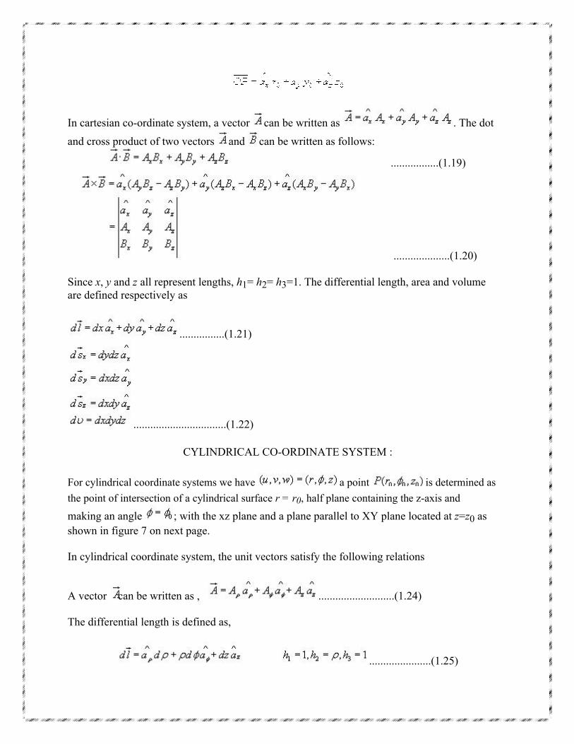
Since x, y and z all represent lengths, h1= h2= h3=1. The differential length, area and volume are defined respectively as

................(1.21)

.................................(1.22)

CYLINDRICAL CO-ORDINATE SYSTEM :

For cylindrical coordinate systems we have a point is determined as

the point of intersection of a cylindrical surface r = r0, half plane containing the z-axis and

making an angle ; with the xz plane and a plane parallel to XY plane located at z=z0 as shown in figure 7 on next page.

In cylindrical coordinate system, the unit vectors satisfy the following relations

A vector can be written as , ...........................(1.24)

The differential length is defined as,

......................(1.25)

.....................(1.23)

Transformation between Cartesian and Cylindrical coordinates:

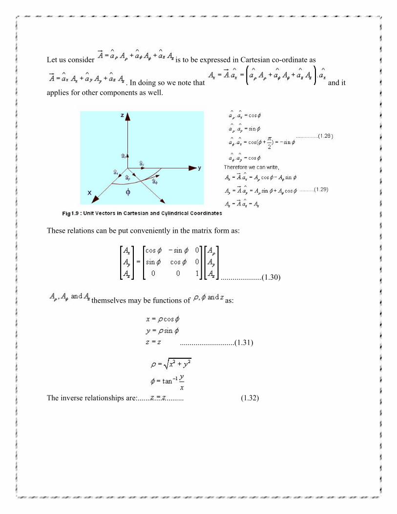
Let us consider is to be expressed in Cartesian co-ordinate as

. In doing so we note that and it applies for other components as well.

These relations can be put conveniently in the matrix form as:

.....................(1.30)

themselves may be functions of as:

............................(1.31)

The inverse relationships are:........................ (1.32)

Fig 1.10: Spherical Polar Coordinate System

Thus we see that a vector in one coordinate system is transformed to another coordinate system through two-step process: Finding the component vectors and then variable transformation.

Spherical Polar Coordinates:

For spherical polar coordinate system, we have, . A point is represented as the intersection of

(i) Spherical surface r=r0

(ii) Conical surface ,and

(iii) half plane containing z-axis making angle with the xz plane as shown in the figure 1.10.

The unit vectors satisfy the following relationships:..................................... (1.33)

The orientation of the unit vectors are shown in the figure 1.11.

A vector in spherical polar co-ordinates is written as : and

For spherical polar coordinate system we have h1=1, h2= r and h3= .

With reference to the Figure 1.12, the elemental areas are:

.......................(1.34)

and elementary volume is given by

........................(1.35)

Coordinate transformation between rectangular and spherical polar:

With reference to the figure 1.13 ,we can write the following equations:

........................................................(1.36)

Given a vector in the spherical polar coordinate system, its component in the cartesian coordinate system can be found out as follows:

.................................(1.37)

Similarly,

.................................(1.38a)

.................................(1.38b)

The above equation can be put in a compact form:

.................................(1.39)

The components themselves will be functions of . are related to x,y and z as:

....................(1.40)

and conversely,

.......................................(1.41a)

.................................(1.41b)

.....................................................(1.41c)

Using the variable transformation listed above, the vector components, which are functions of variables of one coordinate system, can be transformed to functions of variables of other coordinate system and a total transformation can be done.

2. Write short notes on the following :

(i) Gradient

(ii) Divergence

(iii) Curl and

(iv) Stokes Theorem

Gradient of a Scalar function:

Let us consider a scalar field V(u,v,w) , a function of space coordinates.

Gradient of the scalar field V is a vector that represents both the magnitude and direction of the maximum space rate of increase of this scalar field V.

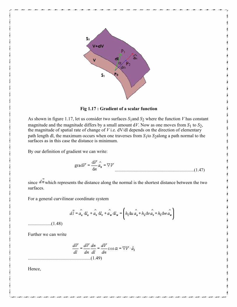
Fig 1.17 : Gradient of a scalar function

As shown in figure 1.17, let us consider two surfaces S1and S2 where the function V has constant magnitude and the magnitude differs by a small amount dV. Now as one moves from S1 to S2, the magnitude of spatial rate of change of V i.e. dV/dl depends on the direction of elementary path length dl, the maximum occurs when one traverses from S1to S2along a path normal to the surfaces as in this case the distance is minimum.

By our definition of gradient we can write:

.......................................................................(1.47)

since which represents the distance along the normal is the shortest distance between the two surfaces.

For a general curvilinear coordinate system

....................(1.48)

Further we can write

......................................................(1.49)

Hence,

....................................(1.50)

Also we can write,

............................(1.51)

By comparison we can write,

....................................................................(1.52)

Hence for the Cartesian, cylindrical and spherical polar coordinate system, the expressions for gradient can be written as:In Cartesian coordinates:

...................................................................................(1.53

) In cylindrical coordinates:

..................................................................(1.54)

and in spherical polar coordinates:

..........................................................(1.55)

The following relationships hold for gradient operator.

...............................................................................(1.56)

where U and V are scalar functions and n is an integer.

It may further be noted that since magnitude of depends on the direction of dl, it is

called the directional derivative. If is called the scalar potential function of the

vector function .

Divergence of a Vector Field:

In study of vector fields, directed line segments, also called flux lines or streamlines, represent field variations graphically. The intensity of the field is proportional to the density of lines. For example, the number of flux lines passing through a unit surface S normal to the vector measures the vector field strength.

Fig 1.18: Flux Lines

We have already defined flux of a vector field as

....................................................(1.57)

For a volume enclosed by a surface,

.........................................................................................(1.58)

We define the divergence of a vector field at a point P as the net outward flux from a volume enclosing P, as the volume shrinks to zero.

.................................................................(1.59)

Here is the volume that encloses P and S is the corresponding closed surface.

Fig 1.19: Evaluation of divergence in curvilinear coordinate

Let us consider a differential volume centered on point P(u,v,w) in a vector field . The flux through an elementary area normal to u is given by ,

........................................(1.60)

Net outward flux along u can be calculated considering the two elementary surfaces perpendicular to u .

.......................................(1.61)

Considering the contribution from all six surfaces that enclose the volume, we can write

.......................................(1.62)

Hence for the Cartesian, cylindrical and spherical polar coordinate system, the expressions for divergence can be written as:

In Cartesian coordinates:

................................(1.63)

In cylindrical coordinates:

....................................................................(1.64)

and in spherical polar coordinates:

......................................(1.65)

In connection with the divergence of a vector field, the following can be noted

Divergence of a vector field gives a scalar.

.............................................................................. (1.66)

Curl of a vector field:

We have defined the circulation of a vector field A around a closed path as .

Curl of a vector field is a measure of the vector field's tendency to rotate about a point.Curl , also written as is defined as a vector whose magnitude is maximum of the net circulation per unit area when the area tends to zero and its direction is the normal

direction to the area when the area is oriented in such a way so as to make the circulation maximum.

Therefore, we can write:

......................................(1.68)

To derive the expression for curl in generalized curvilinear coordinate system, we first

compute and to do so let us consider the figure 1.20 :

Fig 1.20: Curl of a Vector

C1 represents the boundary of , then we can write

......................................(1.69

) The integrals on the RHS can be evaluated as follows:

.................................(1.70)

................................................(1.71)

The negative sign is because of the fact that the direction of traversal reverses. Similarly,

..................................................(1.72)

............................................................................(1.73)

Adding the contribution from all components, we can write:

........................................................................(1.74)

Therefore, ........................(1.75)

In the same manner if we compute for and we can write,

.......(1.76)

This can be written as,

......................................................(1.77)

In Cartesian coordinates:....................................... (1.78)

In Cylindrical coordinates, ....................................(1.79)

In Spherical polar coordinates, ..............(1.80)Curl operation exhibits the following properties:

..............(1.81)

3. State and Derive Divergence and Stoke’s theorem.

Divergence theorem :

Divergence theorem states that the volume integral of the divergence of vector field is equal to the net outward flux of the vector through the closed surface that bounds the volume.

Mathematically,

Proof:

Let us consider a volume V enclosed by a surface S . Let us subdivide the volume in large

number of cells. Let the kTH

cell has a volume and the corresponding surface is denoted

by SK. Interior to the volume, cells have common surfaces. Outward flux through these common surfaces from one cell becomes the inward flux for the neighboring cells. Therefore when the total flux from these cells are considered, we actually get the net outward flux through the surface surrounding the volume. Hence we can write:

......................................(1.67)

In the limit, that is when and the right hand of the expression can be written as

.

Hence we get , which is the divergence theorem.

Stoke's theorem :

It states that the circulation of a vector field around a closed path is equal to the integral of

over the surface bounded by this path. It may be noted that this equality holds provided

and are continuous on the surface.

i.e,

..............(1.82)

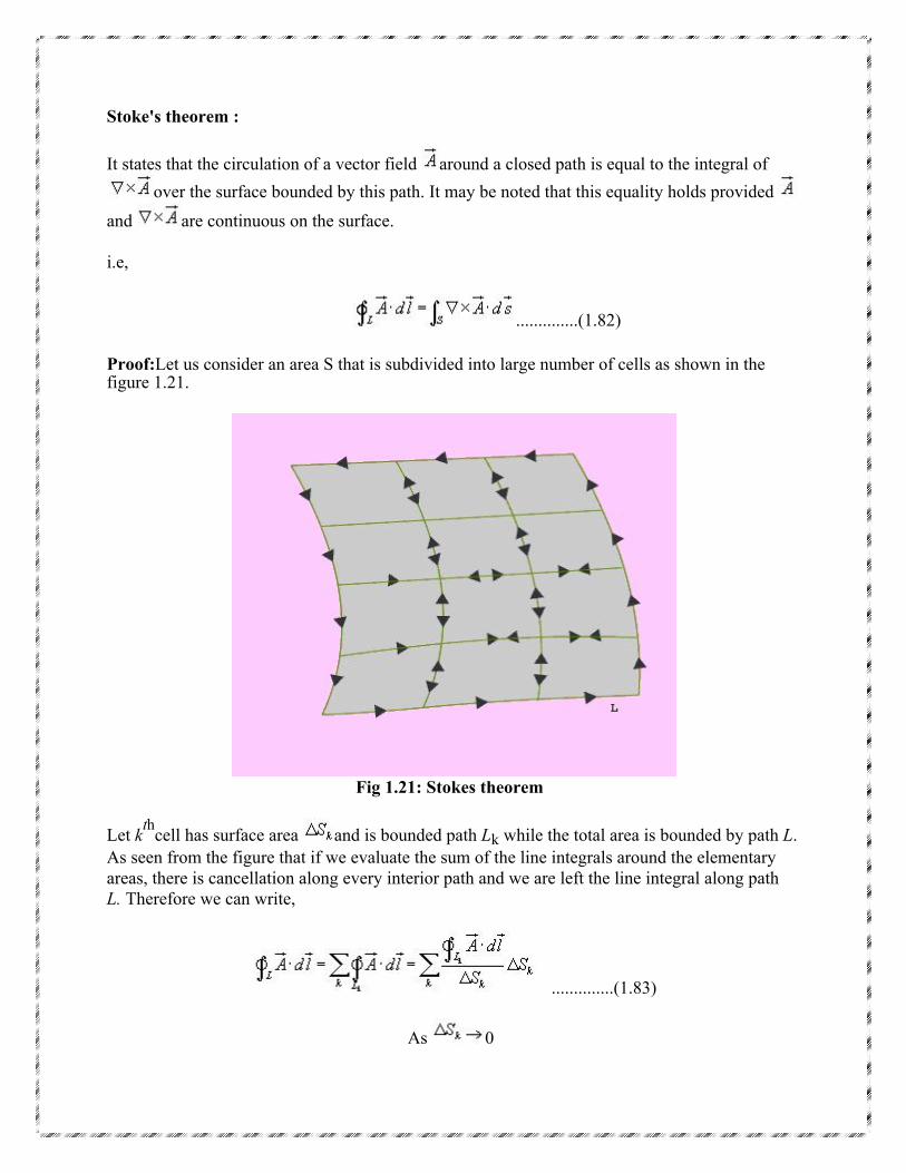
Proof:Let us consider an area S that is subdivided into large number of cells as shown in thefigure 1.21.

Fig 1.21: Stokes theorem

Let kth

cell has surface area and is bounded path Lk while the total area is bounded by path L. As seen from the figure that if we evaluate the sum of the line integrals around the elementary areas, there is cancellation along every interior path and we are left the line integral along path L. Therefore we can write,

..............(1.83)

As 0

. .............(1.84)

which is the stoke's theorem.

Unit-2Electrostatics-2

4. State superposition theorem in relevance to field theory and derive the equation for total electric field intensity.

Electric Field

The electric field intensity or the electric field strength at a point is defined as the force per unit charge. That is

or, .......................................(2.4)

The electric field intensity E at a point R (observation point) due a point charge Q located at (source point) is given by:

..........................................(2.5)

For a collection of N point charges Q1 ,Q2 ,.........QN located at , ,...... , the electric

field intensity at point is obtained as

........................................(2.6)

The expression (2.6) can be modified suitably to compute the electric filed due to a continuous distribution of charges.

In figure 2.2 we consider a continuous volume distribution of charge (T) in the region denoted as the source region.

For an elementary charge , i.e. considering this charge as point charge, we can write the field expression as:

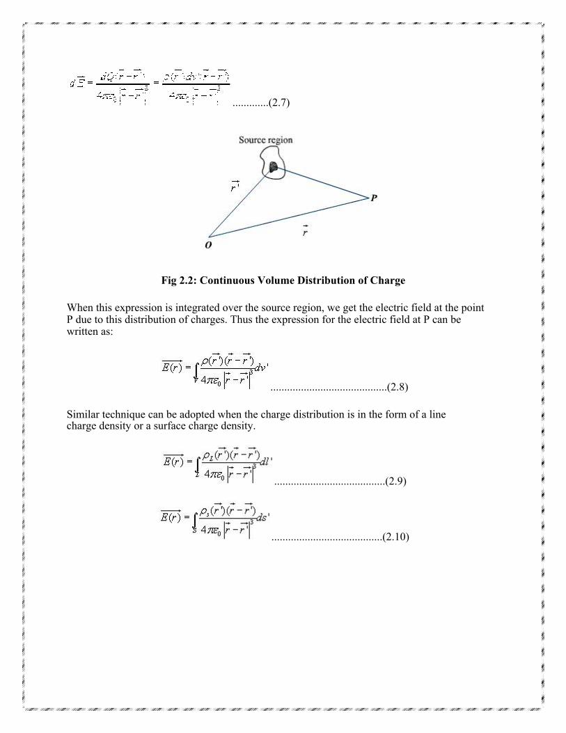
.............(2.7)

Fig 2.2: Continuous Volume Distribution of Charge

When this expression is integrated over the source region, we get the electric field at the point P due to this distribution of charges. Thus the expression for the electric field at P can be written as:

..........................................(2.8)

Similar technique can be adopted when the charge distribution is in the form of a line charge density or a surface charge density.

........................................(2.9)

........................................(2.10)

5. Deduce an expression for the capacitance of a parallel plate capacitor having two dielectric media.

Parallel plate capacitor

Fig 2.20: Parallel Plate Capacitor

For the parallel plate capacitor shown in the figure 2.20, let each plate has area A and a distance h separates the plates. A dielectric of permittivity fills the region between the plates. The electric field lines are confined between the plates. We ignore the flux fringing at the edges of the plates and charges are assumed to be uniformly distributed over the conducting plates with

densities and - , .

By Gauss’s theorem we can write, .......................(2.85)

As we have assumed to be uniform and fringing of field is neglected, we see that E is constant in

the region between the plates and therefore, we can write . Thus, for a parallel

plate capacitor we have,........................(2.86)

Series and parallel Connection of capacitors

Capacitors are connected in various manners in electrical circuits; series and parallel connections are the two basic ways of connecting capacitors. We compute the equivalent capacitance for such connections.

Series Case: Series connection of two capacitors is shown in the figure 2.21. For this case wecan write,

.......................(2.87)

Fig 2.21: Series Connection of Capacitors

Fig 2.22: Parallel Connection of Capacitors

The same approach may be extended to more than two capacitors connected in series.

Parallel Case: For the parallel case, the voltages across the capacitors are the same.

The total charge

Therefore, .......................(2.88)

6. State and derive Poisson’s and Laplace’s Equations

Poisson’s and Laplace’s Equations

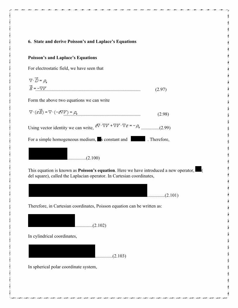
For electrostatic field, we have seen that

.......................................................................................... (2.97)

Form the above two equations we can write

.................................................................. (2.98)

Using vector identity we can write, ................(2.99)

For a simple homogeneous medium, is constant and . Therefore,

................(2.100)

This equation is known as Poisson’s equation. Here we have introduced a new operator, ( del square), called the Laplacian operator. In Cartesian coordinates,

...............(2.101)

Therefore, in Cartesian coordinates, Poisson equation can be written as:

...............(2.102)

In cylindrical coordinates,

...............(2.103)

In spherical polar coordinate system,

...............(2.104)

At points in simple media, where no free charge is present, Poisson’s equation reduces to

...................................(2.105)

which is known as Laplace’s equation.

Unit-3

Magnetostatics

7. State Biot-Savart's Law.

Biot- Savart Law

This law relates the magnetic field intensity DH produced at a point due to a differential current element as shown in Fig. 4.2.

Fig. 4.2: Magnetic field intensity due to a current element

The magnetic field intensity at P can be written as,

............................(4.1a)

..............................................(4.1b)

where is the distance of the current element from the point P.

Similar to different charge distributions, we can have different current distribution such as line current, surface current and volume current. These different types of current densities are shown in Fig. 4.3.

Line Current Surface Current Volume Current

Fig. 4.3: Different types of current distributions

By denoting the surface current density as K (in amp/m) and volume current density as J (in amp/m

2) we can write:

......................................(4.2)

( It may be noted that )

Employing Biot-Savart Law, we can now express the magnetic field intensity H. In terms of these current distributions.

............................. for line current............................ (4.3a)

........................ for surface current .................... (4.3b)

....................... for volume current...................... (4.3c)

To illustrate the application of Biot - Savart's Law, we consider the following example.

8. State and explain Ampere’s circuital law and show that the field strength at the end of a long solenoid is one half of that at the centre.

Ampere's Circuital Law:

Ampere's circuital law states that the line integral of the magnetic field (circulation of H ) around a closed path is the net current enclosed by this path. Mathematically,

......................................(4.8)

The total current I enc can be written as,

......................................(4.9)By applying Stoke's theorem, we can write

......................................(4.10) which is the Ampere's law in the point form.

9. Obtain an expression for the magnetic field intensity due to finite length current carrying conductor.

We consider a finite length of a conductor carrying a current placed along z-axis as shown in the Fig 4.4. We determine the magnetic field at point P due to this current carrying conductor.

Fig. Field at a point P due to a finite length current carrying conductor

With reference to Fig. 4.4, we find that

Applying Biot - Savart's law for the current element

we can write,

Substituting we can write,

We find that, for an infinitely long conductor carrying a current I , and

Therefore,

10. Derive the Boundary Condition for Magnetic Fields.

Boundary Condition for Magnetic Fields:

Similar to the boundary conditions in the electro static fields, here we will consider the behavior

of and at the interface of two different media. In particular, we determine how the tangential and normal components of magnetic fields behave at the boundary of two regions having different permeabilities.

The figure 4.9 shows the interface between two media having permeabities and , being the normal vector from medium 2 to medium 1.

Figure 4.9: Interface between two magnetic media

To determine the condition for the normal component of the flux density vector , we considera small pill box P with vanishingly small thickness H and having an elementary area for the faces. Over the pill box, we can write

....................................................(4.36)

Since h --> 0, we can neglect the flux through the sidewall of the pill box.

...........................(4.37)

and.................. (4.38)

where

and.......................... (4.39)

Since is small, we can write

or, ...................................(4.40)

That is, the normal component of the magnetic flux density vector is continuous across the interface.

In vector form,

...........................(4.41)

To determine the condition for the tangential component for the magnetic field, we consider a closed path C as shown in figure 4.8. By applying Ampere's law we can write

....................................(4.42)

Since h -->0,

...................................(4.43)

We have shown in figure 4.8, a set of three unit vectors , and such that they satisfy

(R.H. rule). Here is tangential to the interface and is the vector perpendicular to the surface enclosed by C at the interface

The above equation can be written as

or, ...................................(4.44)

i.e., tangential component of magnetic field component is discontinuous across the interface where a free surface current exists.

If JS = 0, the tangential magnetic field is also continuous. If one of the medium is a perfect conductor JS exists on the surface of the perfect conductor.

In vector form we can write,

...................................(4.45)

Therefore,

...................................(4.46)

Unit-4

Electrodynamic fields

11. Derive and explain Maxwell’s equations both in integral and point forms.

Maxwell's Equation

Equation (5.1) and (5.2) gives the relationship among the field quantities in the static field. For time varying case, the relationship among the field vectors written as

(5.20a)

(5.20b)

(5.20c)

(5.20d)

In addition, from the principle of conservation of charges we get the equation of continuity

(5.21) The equation 5.20 (a) - (d) must be consistent with equation (5.21).

We observe that

(5.22)

Since is zero for any vector .

Thus applies only for the static case i.e., for the scenario when . A classic example for this is given below .

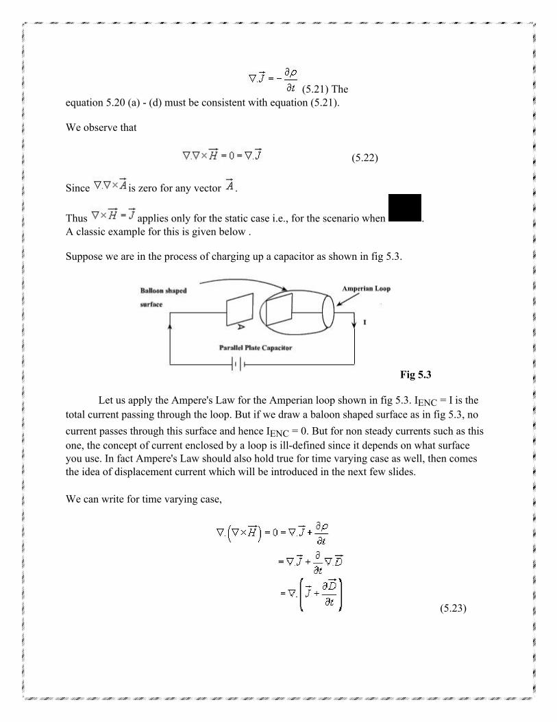
Suppose we are in the process of charging up a capacitor as shown in fig 5.3.

Fig 5.3

Let us apply the Ampere's Law for the Amperian loop shown in fig 5.3. IENC = I is the total current passing through the loop. But if we draw a baloon shaped surface as in fig 5.3, no

current passes through this surface and hence IENC = 0. But for non steady currents such as this one, the concept of current enclosed by a loop is ill-defined since it depends on what surface you use. In fact Ampere's Law should also hold true for time varying case as well, then comes the idea of displacement current which will be introduced in the next few slides.

We can write for time varying case,

(5.23)

(5.24)

The equation (5.24) is valid for static as well as for time varying case.

Equation (5.24) indicates that a time varying electric field will give rise to a magnetic field even

in the absence of . The term has a dimension of current densities and is called thedisplacement current density.

Introduction of in equation is one of the major contributions of Jame's Clerk Maxwell. The modified set of equations

(5.25a)

(5.25b)

(5.25c)

(5.25d)

is known as the Maxwell's equation and this set of equations apply in the time varying scenario,

static fields are being a particular case .

In the integral form

(5.26a)

(5.26b)

(5.26c)

(5.26d)

The modification of Ampere's law by Maxwell has led to the development of a unified electromagnetic field theory. By introducing the displacement current term, Maxwell could predict the propagation of EM waves. Existence of EM waves was later demonstrated by Hertz experimentally which led to the new era of radio communication.

12. Derive and explain Faraday’s Law equations both in integral and point forms.

Faraday's Law of electromagnetic Induction

Michael Faraday, in 1831 discovered experimentally that a current was induced in a conducting loop when the magnetic flux linking the loop changed. In terms of fields, we can say that a time varying magnetic field produces an electromotive force (emf) which causes a current in a closed circuit. The quantitative relation between the induced emf (the voltage that arises from conductors moving in a magnetic field or from changing magnetic fields) and the rate of change of flux linkage developed based on experimental observation is known as Faraday's law. Mathematically, the induced emf can be written as

Emf = Volts (5.3)

where is the flux linkage over the closed path.

A non zero may result due to any of the following:

(a) time changing flux linkage a stationary closed path.

(b) relative motion between a steady flux a closed path.

(c) a combination of the above two cases.

The negative sign in equation (5.3) was introduced by Lenz in order to comply with the polarity of the induced emf. The negative sign implies that the induced emf will cause a current flow in the closed loop in such a direction so as to oppose the change in the linking magnetic flux which produces it. (It may be noted that as far as the induced emf is concerned, the closed path forming a loop does not necessarily have to be conductive).

If the closed path is in the form of N tightly wound turns of a coil, the change in the magnetic flux linking the coil induces an emf in each turn of the coil and total emf is the sum of the induced emfs of the individual turns, i.e.,

Emf = Volts (5.4)

By defining the total flux linkage as

(5.5)

The emf can be written as

Emf = (5.6)

Continuing with equation (5.3), over a closed contour 'C' we can write

Emf = (5.7)

where is the induced electric field on the conductor to sustain the current.

Further, total flux enclosed by the contour 'C ' is given by

(5.8)

Where S is the surface for which 'C' is the contour.

From (5.7) and using (5.8) in (5.3) we can write

(5.9)

By applying stokes theorem

(5.10)

Therefore, we can write

(5.11)

which is the Faraday's law in the point form

We have said that non zero can be produced in a several ways. One particular case is when a time varying flux linking a stationary closed path induces an emf. The emf induced in a stationary closed path by a time varying magnetic field is called a transformer emf .

Unit-5

Electromagnetic waves

13. Explain in detail the behavior of plane waves in lossless medium.

Plane waves in Lossless medium:

In a lossless medium, are real numbers, so k is real.

In Cartesian coordinates each of the equations 6.1(a) and 6.1(b) are equivalent to three scalar Helmholtz's equations, one each in the components Ex, E y and Ez or Hx , Hy, Hz.

For example if we consider Ex component we can write

.................................................(6.1)

A uniform plane wave is a particular solution of Maxwell's equation assuming electric field (and magnetic field) has same magnitude and phase in infinite planes perpendicular to the direction of propagation. It may be noted that in the strict sense a uniform plane wave doesn't exist in practice as creation of such waves are possible with sources of infinite extent. However, at large distances from the source, the wavefront or the surface of the constant phase becomes almost spherical and a small portion of this large sphere can be considered to plane. The characteristics of plane waves are simple and useful for studying many practical scenarios.

Let us consider a plane wave which has only Ex component and propagating along z . Since the plane wave will have no variation along the plane perpendicular to z i.e., xy plane,

. The Helmholtz's equation (6.2) reduces to,

.........................................................................(6.2)

The solution to this equation can be written as

............................................................(6.3)

are the amplitude constants (can be determined from boundary conditions).

In the time domain,

.............................(6.4)

assuming are real constants.

Here, represents the forward traveling wave. The plot of for several values of t is shown in the Figure 6.1.

Figure 6.1: Plane wave traveling in the + Z direction

As can be seen from the figure, at successive times, the wave travels in the +z direction.

If we fix our attention on a particular point or phase on the wave (as shown by the dot) i.e. , = constant

Then we see that as T is increased to , z also should increase to so that

Or,

Or,

When ,

we write = phase velocity .

.....................................(6.5)

If the medium in which the wave is propagating is free space i.e.,

Then

Where 'C' is the speed of light. That is plane EM wave travels in free space with the speed of light.

The wavelength is defined as the distance between two successive maxima (or minima or any other reference points).

i.e.,

or,

or,

Substituting ,

or, ................................(6.6)

Thus wavelength also represents the distance covered in one oscillation of the wave. Similarly,

represents a plane wave traveling in the -z direction.

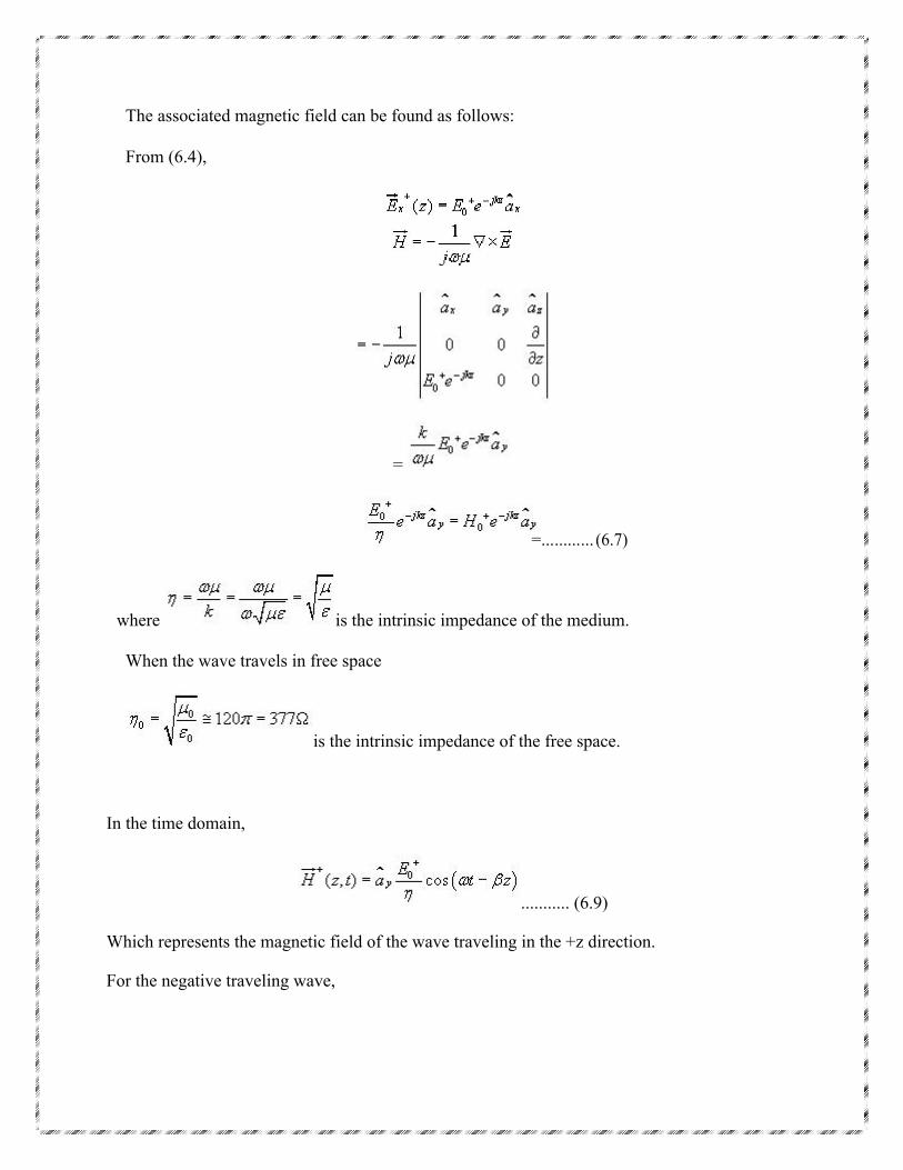
The associated magnetic field can be found as follows:

From (6.4),

=

=............ (6.7)

where is the intrinsic impedance of the medium.

When the wave travels in free space

is the intrinsic impedance of the free space.

In the time domain,

........... (6.9)

Which represents the magnetic field of the wave traveling in the +z direction.

For the negative traveling wave,

...........(6.10)

For the plane waves described, both the E & H fields are perpendicular to the direction of propagation, and these waves are called TEM (transverse electromagnetic) waves.

The E & H field components of a TEM wave is shown in Fig 6.2.

Figure 6.2 : E & H fields of a particular plane wave at time t.

14. Explain Poynting Vector and Power Flow in ElectromagneticFields.

Poynting Vector and Power Flow in Electromagnetic Fields:

Electromagnetic waves can transport energy from one point to another point. The electric and magnetic field intensities asscociated with a travelling electromagnetic wave can be related to the rate of such energy transfer.

Let us consider Maxwell's Curl Equations:

Using vector identity

the above curl equations we can write

.............................................(6.35)

In simple medium where and are constant, we can write

and

Applying Divergence theorem we can write,

...........................(6.36)

The term represents the rate of change of energy stored in the electric

and magnetic fields and the term represents the power dissipation within the volume. Hence right hand side of the equation (6.36) represents the total decrease in power within the volume under consideration.

The left hand side of equation (6.36) can be written as where

(W/mt2) is called the Poynting vector and it represents the power density vector associated with the

electromagnetic field. The integration of the Poynting vector over any closed surface gives the net power flowing out of the surface. Equation (6.36) is referred to as Poynting theorem and

it states that the net power flowing out of a given volume is equal to the time rate of decrease in the energy stored within the volume minus the conduction losses.