HAL Id: hal-00327496https://hal.archives-ouvertes.fr/hal-00327496

Preprint submitted on 8 Oct 2008

HAL is a multi-disciplinary open accessarchive for the deposit and dissemination of sci-entific research documents, whether they are pub-lished or not. The documents may come fromteaching and research institutions in France orabroad, or from public or private research centers.

L’archive ouverte pluridisciplinaire HAL, estdestinée au dépôt et à la diffusion de documentsscientifiques de niveau recherche, publiés ou non,émanant des établissements d’enseignement et derecherche français ou étrangers, des laboratoirespublics ou privés.

Uniqueness results for convex Hamilton-Jacobiequations under p > 1 growth conditions on data

Francesca da Lio, Olivier Ley

To cite this version:Francesca da Lio, Olivier Ley. Uniqueness results for convex Hamilton-Jacobi equations under p > 1growth conditions on data. 2008. hal-00327496

Uniqueness results for convex Hamilton-Jacobi equations under

p > 1 growth conditions on data

Francesca Da Lio(1) & Olivier Ley(2)

October 8, 2008

Abstract

Unbounded stochastic control problems may lead to Hamilton-Jacobi-Bellman equationswhose Hamiltonians are not always defined, especially when the diffusion term is unboundedwith respect to the control. We obtain existence and uniqueness of viscosity solutions growingat most like o(1 + |x|p) at infinity for such HJB equations and more generally for degenerateparabolic equations with a superlinear convex gradient nonlinearity. If the correspondingcontrol problem has a bounded diffusion with respect to the control, then our results applyto a larger class of solutions, namely those growing like O(1 + |x|p) at infinity. This lattercase encompasses some equations related to backward stochastic differential equations.

Keywords. degenerate parabolic equations, Hamilton-Jacobi-Bellman equations, viscosity solutions, un-

bounded solutions, maximum principle, backward stochastic differential equations, unbounded stochastic

control problems.

AMS subject classifications. 35K65, 49L25, 35B50, 35B37, 49N10, 60H35.

1 Introduction

In the joint paper [13] the authors obtain a comparison result between semicontinuous viscositysolutions, neither bounded from below nor from above, growing at most quadratically in thestate variable, of second order degenerate parabolic equations of the form

∂u

∂t+H(x, t,Du,D2u) = 0 in IRN × (0, T ),

u(x, 0) = ψ(x) in IRN ,

(1)

where N ≥ 1, T > 0. The unknown u is a real-valued function defined in IRN × [0, T ], Du andD2u denote respectively its gradient and Hessian matrix and ψ is a given initial condition. TheHamiltonian H : IRN × [0, T ] × IRN × SN (IR) → IR has the form

H(x, t, q,X) = supα∈A

−〈b(x, t, α), q〉 − ℓ(x, t, α) − Trace[

σ(x, t, α)σT (x, t, α)X]

. (2)

(1)Dipartimento di Matematica Pura e Applicata, Via Trieste, 63, 35121 Padova, Italy.(2)Laboratoire de Mathematiques et Physique Theorique (UMR CNRS 6083). Federation Denis Poisson

(FR 2964). Universite Francois Rabelais Tours. Parc de Grandmont, 37200 Tours, France.

1

Note that H is convex with respect to q. The key assumptions in the paper [13] are that A is anunbounded control set, the functions b and ℓ grow respectively at most linearly and quadraticallywith respect to both the control and the state. Instead the functions σ is assumed to grow atmost linearly with respect to the state and is bounded with respect to the control. (In fact,in [13], we consider more general equations of Isaacs type by adding a concave Hamiltonian Gwith bounded control, see Remark 2.1. To simplify the exposition we take G ≡ 0 here.)

In the present work, we extend the results of [13] in two directions.

The first issue is to obtain a comparison result for unbounded solutions under the weakerassumption that the diffusion matrix σ is unbounded also with respect to the control. The maindifficulty is that the Hamiltonian H may not be continuous. To illustrate this fact, consider forinstance the case where A = IRN , b = α, σ = |α|I and ℓ = |α|2. The Hamiltonian H becomes

supα∈IRN

−〈α,Du〉 − |α|2 − |α|22

∆u, (3)

which is +∞ as soon as ∆u < −2. This example is motivated by the well-known StochasticLinear Quadratic problem, see for instance Bensoussan [8], Fleming and Rishel [15], Flemingand Soner [16], Øksendal [22], Yong and Zhou [25] and the references therein for an overviewof this problem. The usual way to deal with such a problem is to plug into the equationvalue functions V of particular form (for instance quadratic in space) for which one knows thatH(x, t, V,DV ) is defined. It leads to some ordinary differential equations of Ricatti type whichallow to identify precisely the value function (see [25]). Another way is to replace the Hamilton-Jacobi-Bellman equation by a variational inequality, see Barles [5] for instance. Our aim is tostudy directly the PDE (1) without any a priori knowledge on the value function. Indeed, forgeneral datas, one does not expect explicit formula for the value function.

We overcome the above difficulty in noticing that it is possible to formulate the definition ofviscosity solutions for HJB in a new way without writing the “sup” in (2), see Definition 2.1. Itprovides a precise definition of solutions for (1) even in cases like (3). Let us stress that it is nota new definition of viscosity solutions but only a new formulation. Using this formulation, weprove a comparison result for solutions in the class of functions growing at most like o(1 + |x|p)at infinity. It provides new results for Stochastic Linear Quadratic type problems (in this case,p = 2) but, unfortunately, we are not able to treat the classical Stochastic Linear Quadratic typeproblem with terminal cost ψ(x) = |x|2 since it requires a comparison in the class O(1 + |x|2).Nevertheless, our results apply to very general datas (not only polynomials of degree 1 or 2 in(x, α)), see Example 2.1.

The second issue of our work is to extend the results of [13] for p-growth type conditions onthe datas and the solutions and for more general equations with an additional nonlinearity fwhich is also convex with respect to the gradient and depends on u. The motivation comes fromPDEs arising in the context of backward stochastic differential equations (BSDEs in short).

In the framework of BSDEs, one generally considers forward-backward systems of the form

dXx,ts = b(Xx,t

s , s)ds + σ(Xt,xs , s)dWs, t ≤ s ≤ T,

Xt,xt = x,

(4)

2

−dY x,ts = f(Xx,t

s , s, Y x,ts , Zx,t

s )ds− Zx,ts dWs, t ≤ s ≤ T,

Y x,tT = ψ(x),

(5)

where (Ws)s∈[0,T ] is standard Brownian motion on a probability space (Ω,F , (Ft)t∈[0,T ], P ), with(Ft)t∈[0,T ] the standard Brownian filtration. (Note that b and σ do not depend on the control).The diffusion (4) is associated with the second-order elliptic operator L defined by

Lu = −1

2Trace(σσTD2u) − 〈b(x, t),Du〉.

The forward-backward system (4)-(5) is formally connected to the PDE

−∂u∂t

+ Lu− f(x, t, u, s(x, t)Du) = 0 in IRN × (0, T )

u(x, T ) = ψ(x) in IRN .

(6)

by the nonlinear Feynman-Kac formula

u(x, t) = Y x,tt for all (x, t) ∈ IRN × [0, T ]. (7)

We recall that nonlinear BSDEs with Lipschitz continuous coefficients were first introduced byPardoux and Peng [23], who proved existence and uniqueness. Their results were extended byKobylanski [20] for bounded solutions in the case of coefficients f having a quadratic growthin the gradient. Briand and Hu [9] generalized this latter result to the case of solutions whichare O(1 + |x|p), as |x| → ∞, with 1 ≤ p < 2. In all these works, the connection with viscositysolutions to the related PDE (6) is established: u defined by (7) is a viscosity solution of (6).

Our aim is to prove the analytical counterpart of their results. More precisely, we want toprove the existence and uniqueness of the solution of (6) under the assumptions of [9].

Let us turn to a more precise description of our results. We consider equations of the form

∂u

∂t+H(x, t,Du,D2u) + f(x, t, u, s(x, t)Du) = 0 in IRN × (0, T ),

u(x, 0) = ψ(x) in IRN ,

(8)

where H is given by (2) with A unbounded, f : IRN × [0, T ]×IRN → IR is continuous and convexin the gradient and s is bounded. We look for solutions with p > 1 growth assumptions (see (12)and (39)) and both H and f satisfies some p′ growth assumptions, where p′ = p/(p − 1) is theconjugate of p. See (A), (B), (C) for the precise assumptions. Let us mention that the typicalcase we want to deal with is

f(x, t, u, s(x, t)Du) = |s(x, t)Du|p′ , p′ > 1,

and the presence of x in the power-p′ term is delicate to treat (especially when doubling thevariables in viscosity type’s proofs, see the proof of Lemma 3.2). The u-dependence in f meansthat f(x, t, u, s(x, t)Du) may not be on the form of H and induces some technical difficulties.

Section 2 is devoted to the case with diffusion matrices σ which depend on the control inan unbounded way, see condition (9). The compensation to this condition with respect to [13]

3

(where σ was assumed to be bounded with respect to the control and p = 2) is that we provethe comparison result Theorem 2.1 for semicontinuous sub- and supersolutions of (8) growing atmost like o(1+|x|p) as |x| → ∞ (instead of O(1+|x|2) in [13]). So far it remains an open questionto know if there is uniqueness in the larger class O(1+ |x|p). The proof of the comparison resultrelies on classical techniques of viscosity solutions. We build a suitable test-function and provesome fine estimates on the various terms which appear, the main difficulty consists in dealingwith the unbounded control terms.

In Section 3, we extend the comparison result in [13] for equations with p > 1 growthconditions on the datas (instead of quadratic growth) with the additional nonlinearity f. Onemotivation to add the nonlinearity f comes from the BSDEs (where s = σ) since the mainapplication of Theorem 3.1 is the uniqueness for the equation stated in [9] (see Example 3.2).In this case, we consider Hamiltonians H with α-bounded diffusion matrices σ, so we choose toreplace (8) by the control independent PDE (38) to simplify the exposition. The control casedoes not present additional difficulties with respect to [13, Theorem 2.1]. The main difficultyin the proof of Theorem 3.1 is to be able to deal with solutions growing like O(1 + |x|p) (whichare not bounded neither from above nor from below). The strategy of proof is similar to theone used in [13] which consists essentially in the following three steps. First one computes theequation satisfied by wµ = µu− v, being u, v respectively the subsolution and the supersolutionof the original PDE and 0 < µ < 1 a parameter. Then for all R > 0 one constructs a strictsupersolution ΦR

µ of the “linearized equation” such that ΦRµ (x, t) → 0 as R → +∞. Finally one

shows that wµ ≤ ΦRµ and one concludes by letting first R→ +∞ and then µ→ 1.

A by-product of the comparison results obtained in Sections 2 and 3 and Perron’s Methodof Ishii [17] is the existence and uniqueness of a continuous solution to (8) which is respectivelyo(1 + |x|p) and O(1 + |x|p) as |x| → ∞. However, under our general assumptions one cannotexpect the existence of a solution for all times as Example 3.4 shows.

Let us compare our results with related ones in the literature for such kind of Hamilton-Jacobi equations. Uniqueness and existence problems for a class of first-order Hamiltonianscorresponding to unbounded control sets and under assumptions including deterministic linearquadratic problems have been addressed by several authors, see, e.g. the book of Bensoussan [8],the papers of Alvarez [2], Bardi and Da Lio [4], Cannarsa and Da Prato [10], Rampazzo andSartori [24] in the case of convex operators, and the papers of Da Lio and McEneaney [14] andIshii [18] for more general operators. As for second-order Hamiltonians under quadratic growthassumptions, Ito [19] obtained the existence of locally Lipschitz solutions to particular equationsof the form (1) under more regularity conditions on the data, by establishing a priori estimates onthe solutions. Whereas Crandall and Lions in [12] proved a uniqueness result for very particularoperators depending only on the Hessian matrix of the solution. In the case of quasilineardegenerate parabolic equations, existence and uniqueness results for viscosity solutions whichmay have a quadratic growth are proved in [7]. The results which are the closest to ourswere obtained in the following works. Alvarez [1] addressed the case of stationary less generalequations (see Example 3.1). Krylov [21] succeeded in dealing with equations encompassingthe classical Stochastic Linear Quadratic problem but his assumptions are designed to handleexactly this case (cf. Example 2.1 and the discussion therein). Finally Kobylanski [20] studiedalso (8) under quite general assumptions on the datas but for bounded solutions. It seems to be

4

difficult to obtain such a generality in the case of unbounded solutions since her proof is basedon changes of functions of the form u→ −e−u which do not work for solutions which are neitherbounded from below nor from above.

The rigorous connection between control problems and Hamilton-Jacobi-Bellman equations isnot addressed in this paper. In the framework of unbounded controls it may be rather delicate.Some results in this direction were obtained for infinite horizon in the deterministic case byBarles [5] and in the stochastic case by Alvarez [1, 2], Krylov [21] and by the authors [13].

Finally, let us mention that the convexity of the operator with respect to the gradient iscrucial in our proofs. The case of Hamiltonians which are neither convex nor concave (which, inthe case of Equations (16), amounts to take both the control sets A and B unbounded) is alsoof interest and it is a widely open subject. Some results in this direction were obtained in [13,Section 4], for instance in the case of first order equations of the form

∂u

∂t+ h(x, t)|Du|2 = 0 in IRN × [0, T ],

where h(x, t) may change sign and u has a quadratic growth. In a forthcoming paper we aregoing to investigate this issue for more general quadratic non convex-non concave equations.

Throughout the paper we will use the following notations. For all integer N,M ≥ 1 we denoteby MN,M (IR) (respectively SN (IR), S+

N (IR)) the set of real N ×M matrices (respectively realsymmetric matrices, real symmetric nonnegative N ×N matrices). For the sake of notations, allthe norms which appear in the sequel are denoting by | · |. The standard Euclidean inner productin IRN is written 〈·, ·〉. We recall that a modulus of continuity m : IR → IR+ is a nondecreasingcontinuous function such that m(0) = 0. We set B(0, R) = x ∈ IRN : |x| < R. Finally forany O ⊆ IRK , we denote by USC(O) the set of upper semicontinuous functions in O and byLSC(O) the set of lower semicontinuous functions in O. Given p > 1 we will denote by p′ itsconiugate, namely

1

p+

1

p′= 1.

Acknowledgments. Part of this work was done while the second author was a visitor atthe FIM at the ETH in Zurich in January 2007. He would like to thank the Department ofMathematics for his support. We thank Guy Barles for useful comments on the first version ofthis paper.

2 Hamilton-Jacobi-Bellman equations with unbounded diffusion

in the control

In this Section we prove a comparison result for second-order fully nonlinear partial differentialequations of the form (8). The main difference with respect to the result in [13] is that herewe suppose that the diffusion matrix σ depends in a unbounded way in the control (see condi-tion (9)). The compensation to the condition (9) is that we are able to get the uniqueness resultin the smaller class of functions which are o(1 + |x|p) as |x| → ∞ (see (12)).

We list below the main assumptions on H and f .

(A) (Assumption on H) :

5

(i) A is a subset of a separable complete normed space. The main point here is the possibleunboundedness of A.

(ii) b ∈ C(IRN ×[0, T ]×A; IRN ) and there exists Cb > 0 such that, for all x, y ∈ IRN , t ∈ [0, T ],α ∈ A,

|b(x, t, α) − b(y, t, α)| ≤ Cb(1 + |α|)|x − y|,|b(x, t, α)| ≤ Cb(1 + |x| + |α|) ;

(iii) ℓ ∈ C(IRN × [0, T ]×A; IR) and, there exist p > 1 and Cℓ, ν > 0 such that, for all x ∈ IRN ,t ∈ [0, T ], α ∈ A,

Cℓ(1 + |x|p + |α|p) ≥ ℓ(x, t, α) ≥ ν|α|p − Cℓ(1 + |x|p)

and for every R > 0, there exists a modulus of continuity mR such that for all x, y ∈B(0, R), t ∈ [0, T ], α ∈ A,

|ℓ(x, t, α) − ℓ(y, t, α)| ≤ (1 + |α|p)mR(|x− y|) ;

(iv) σ ∈ C(IRN × [0, T ] × A;MN,M (IR)) is Lipschitz continuous with respect to x with aconstant independent of (t, α): namely, there exists Cσ > 0 such that, for all x, y ∈ IRN

and (t, α) ∈ [0, T ] ×A,|σ(x, t, α) − σ(y, t, α)| ≤ Cσ|x− y|,

and satisfies for every x ∈ IRN , t ∈ [0, T ], α ∈ A,

|σ(x, t, α)| ≤ Cσ(1 + |x| + |α|). (9)

(B) (Assumption on f)f ∈ C([0, T ] × IRN × IR × IRN ; IR) and, for all R > 0, there exist a modulus of continuity mR

and Cs, C > 0 such that, for all t ∈ [0, T ], x, y ∈ IRN , u, v ∈ IR, z ∈ IRN ,

(i) |f(x, t, u, z)| ≤ Cf (1 + |x|p + |u| + |z|p′),(ii) |f(x, t, u, z) − f(y, t, u, z)| ≤ mR((1 + |u| + |z|)|x − y|) if |x| + |y| ≤ R,

(iii) z 7→ f(x, t, u, z) is convex,

(iv) s ∈ C(IRN × [0, T ];MN ), |s(x, t) − s(y, t)| ≤ Cs|x− y|, |s(x, t)| ≤ Cs,

(v) |f(x, t, u, z) − f(x, t, v, z)| ≤ C|u− v|.

The typical case we have in mind in the context of (A)(iv) (σ not bounded with respect tothe control) is

σ(x, t, α) = Q(t)x+R(t)α,

where Q(t) and R(t) are matrices of suitable sizes. This case includes Linear Quadratic controlproblems, see Example 2.1.

Under the current hypotheses, the Hamiltonian H may be infinite (see Example 2.1) and forthis reason we re-formulate the definition of viscosity solution in the following way.

6

Definition 2.1(i) A function u ∈ USC(IRN×[0, T ]) is a viscosity subsolution of (8) if for all (x, t) ∈ IRN×[0, T ]and ϕ ∈ C2(IRN × [0, T ]) such that u − ϕ has a maximum at (x, t), we have u(x, t) ≤ ψ(x) ift = 0 and, if t > 0, then

∂ϕ

∂t(x, t) +H(x, t,Dϕ(x, t),D2ϕ(x, t)) + f(x, t, u(x, t), s(x, t)Dϕ(x, t)) ≤ 0,

which is equivalent to: for all α ∈ A,

∂ϕ

∂t(x, t) − 〈b(x, t, α),Dϕ(x, t)〉 − ℓ(x, t, α) − Trace

[

σ(x, t, α)σT (x, t, α)D2ϕ(x, t)]

+ f(x, t, u(x, t), s(x, t)Dϕ(x, t)) ≤ 0. (10)

(ii) A function u ∈ USC(IRN × [0, T ]) is a viscosity supersolution of (8) if for all (x, t) ∈IRN × [0, T ] and ϕ ∈ C2(IRN × [0, T ]) such that u − ϕ has a minimum at (x, t), we haveu(x, t) ≥ ψ(x) if t = 0 and, if t > 0, then for all η > 0, there exists αη = α(η, x, t) ∈ A, suchthat

∂ϕ

∂t(x, t) − 〈b(x, t, αη),Dϕ(x, t)〉 − ℓ(x, t, αη) − Trace

[

σ(x, t, αη)σT (x, t, αη)D

2ϕ(x, t)]

+ f(x, t, u(x, t), s(x, t)Dϕ(x, t)) ≥ −η. (11)

(iii) A locally bounded function u : IRN × [0, T ] → IR is a viscosity solution of (8) if its USCenvelope u∗ is a subsolution and its LSC envelope u∗ is a supersolution.

Note that (10) and (11) is only a way to write the definition of sub- and supersolutions withoutwriting a supremum which could not exist because of assumption (9).

We say that a function u : IRN × [0, T ] → IR is in the class Cp if

u(x, t)

1 + |x|p −→|x|→+∞

0, uniformly with respect to t ∈ [0, T ]. (12)

Note that u ∈ Cp if and only if, for all ε > 0, there exists Mε > 0 such that

|u(x, t)| ≤Mε + ε(1 + |x|p) for all (x, t) ∈ IRN × [0, T ].

In particular, for all λ > 0,

supx∈IRN

u(x, t) − λ(1 + |x|p) = Mλ < +∞. (13)

The main result of this Section is the

Theorem 2.1 Assume (A)-(B) and suppose that ψ is a continuous function which belongs toCp. Let u ∈ USC(IRN × [0, T ]) be a viscosity subsolution of (8) and v ∈ LSC(IRN × [0, T ]) bea viscosity supersolution of (8). Suppose that U and V are in the class Cp defined by (12) andsatisfy u(x, 0) ≤ ψ(x) ≤ v(x, 0). Then u ≤ v in IRN × [0, T ].

7

Before giving the proof of the theorem, let us state an existence result and some examplesof applications. As it was already observed in [13], the question of the existence of a continuoussolution to (1) is not completely obvious and in general the solutions may exist only for short time(see Example 3.4). One way to obtain the existence is to establish a link between the solutionof the PDE and related control problems or BDSE systems which have a solution. By usingPDE methods, in the framework of viscosity solutions, the existence is usually a consequence ofthe comparison principle by means of Perron’s method, as soon as we can build a sub- and asuper-solution to the problem. Here, the comparison principle is proved in the class of functionsbelonging to Cp. Therefore, to prove the existence, it siffices to build sub- and super-solutionsto (38) in Cp. We need to strengthen (A)(iii) and (B)(i) by assuming that ℓ(·, t, α), f(·, t, u, z) ∈Cp uniformly with respect to α, t, u, z, i.e., for all (x, t, α, u, z) ∈ IRN × [0, T ] ×A× IR× IRN ,

χ(x) ≥ ℓ(x, t, α) ≥ ν|α|p − χ(x), |f(x, t, u, z)| ≤ Cf (1 + γ(x) + |u| + |z|p′),and lim

|x|→+∞

χ(x)

1 + |x|p ,γ(x)

1 + |x|p = 0.(14)

We have

Theorem 2.2 Assume (A)–(B) and (14). For all ψ ∈ Cp, there is τ > 0 such that thereexist a subsolution u ∈ Cp and a supersolution u ∈ Cp of (8) in IRN × [0, T ]. In consequence,Equation (8) has a unique continuous viscosity solution in IRN × [0, τ ] in the class Cp.

The proof of this theorem is postponed at the end of the section.

Example 2.1 (A Stochastic Linear Quadratic Control Problem) Consider the stochas-tic differential equation (in dimension 1 for sake of simplicity)

dXs = Xsds+√

2αsdWs, t ≤ s ≤ T, t ∈ (0, T ],X0 = x ∈ IR,

where Ws is a standard Brownian motion, (αs)s is a real valued progressively measurable processand the value function is given by

V (x, t) = inf(αs)s

Etx

∫ T

t|αs|2 ds+ ψ(XT )

.

(Note that in this case, p = p′ = 2.) The Hamilton-Jacobi equation formally associated to thisproblem is

−ut + supα∈IR

−α2(u′′ + 1) − xu′ = 0 in IR× (0, T ],

u(x, T ) = ψ(x) in IR.(15)

We observe that in this case if u′′ + 1 < 0 then the Hamiltonian becomes +∞. Nevertheless, weare able to prove comparison (15) as soon as the terminal cost ψ ∈ Cp (i.e., has a strictly sub-pgrowth). This is not completely satisfactory since, in the classical Linear Quadratic ControlProblem, one expects to have quadratic terminal costs like ψ(x) = |x|2. Let us mention that

8

Krylov [21] succeeded in treating this latter case. But his proof consists on some algebraiccomputations which rely heavily on the particular form of the datas (the datas are supposed tobe polynomials of degree 1 or degree 2 in (x, α)). In our case, up to restrict slightly the growth,we are able to deal with general datas.

Remark 2.1 Theorems 2.1 and 3.1 still hold for the Isaacs equation of [13],

∂u

∂t+H(x, t,Du,D2u) +G(x, t,Du,D2u) + f(x, t, u, s(x, t)Du) = 0 (16)

where

G(x, t, q,X) = infβ∈B

−〈g(x, t, β), q〉 − l(x, t, β) − Trace[

c(x, t, β)cT (x, t, β)X]

,

is a concave Hamiltonian, B is bounded, g, l, c satisfy respectively (A)(ii),(iii),(iv) (with boundedcontrols β). The case where both the control sets A and B are unbounded is rather delicate. Itis the aim of a future work.

Let us turn to the proof of the comparison theorem.

Proof of Theorem 2.1. We are going to show that for every µ ∈ (0, 1), µu − v ≤ 0, inIRN ×[0, T ]. To this end we argue by contradiction assuming that there exists (x, t) ∈ IRN ×[0, T ]such that

u(x, t) − v(y, t) > δ > 0. (17)

We divide the proof in several steps.

1. The µ-equation for the subsolution. If u is a subsolution of (8), then u = µu is a subsolutionof

ut + supα∈A

−Trace(

σ(x, t, α)σ(x, t, α)TD2u)

+ 〈b(x, t, α),Du〉 − µℓ(x, t, α)

+µf(

x, t,1

µu(x, t),

1

µs(x, t)Du) ≤ 0,

with the initial condition µu(x, 0) ≤ µψ(x).

2. Test-function and estimates on the penalization terms. For all ε > 0, η > 0 and θ, L > 0 (tobe chosen later) we consider the auxiliary function

Φ(x, y, t) = µu(x, t) − v(y, t) − eLt( |x− y|2

ε2+ θ(1 − µ)(1 + |x|2 + |y|2)p/2

)

− ρt.

Since u, v ∈ Cp, the supremum of Φ in IRN × IRN × [0, T ] is achieved at a point (x, y, t). We willdrop for simplicity of notation the dependence on the various parameters. If θ and ρ are smallenough we have

Φ(x, y, t) ≥ µu(x, y) − v(x, y) − θ(1 − µ)(1 + 2|x|p) − ρt >δ

2,

9

which implies

|x− y|2ε2

+ θ(1 − µ)(1 + |x|2 + |y|2)p/2 ≤ µu(x, t) − v(y, t).

Therefore, by (13), we get

|x− y|2ε2

+ θ1 − µ

2(1 + |x|2 + |y|2)p/2

≤ sup(x,t)∈IRN×[0,T ]

µu(x, t) − θ1 − µ

2(1 + |x|p)

+ sup(x,t)∈IRN×[0,T ]

−v(x, t) − θ1 − µ

2(1 + |x|p)

≤ M

for some 0 < M = M(µ, θ, u, v). Thus

|x|, |y| ≤ Rµ,θ (18)

with Rµ,θ independent of ε and |x − y| → 0 as ε → 0. Up to extract a subsequence, we canassume that

x, y → x0 ∈ B(0, Rµ,θ), t→ t0 as ε→ 0 (19)

Actually we can obtain a more precise estimate: we have

Φ(x, y, t) ≥ maxIRN×[0,T ]

µu(x, t) − v(x, t) − eLtθ(1 − µ)(1 + 2|x|2)p/2 − ρt := Mµ,θ.

Thus

lim infε→0

Φ(x, y, t) ≥Mµ,θ.

On the other hand

lim supε→0

Φ(x, y, t)

≤ lim supε→0

[µu(x, t)−v(y, t) − eLtθ(1−µ)(1 + |x|2 + |y|2)p/2−ρt] − lim infε→0

eLt |x−y|2ε2

≤Mµ,θ − lim infε→0

eLt |x− y|2ε2

.

By combining the above inequalities we get, up to subsequences, that

|x− y|2ε2

→ 0 as ε→ 0. (20)

Note that we have

|x− y|, |x− y|2ε2

= m(ε), (21)

10

where m denotes a modulus of continuity independent of ε (but which depends on θ, µ).

3. Ishii matricial theorem and viscosity inequalities. We set

Θ(x, y, t) = eLt( |x− y|2

ε2+ θ(1 − µ)(1 + |x|2 + |y|2)p/2

)

+ ρt.

We claim that there is a subsequence εn such that t = 0. Suppose by contradiction that for allε > 0 we have t > 0. Next Steps are devoted to prove some estimates in order to obtain thedesired contradiction at the end of Step 8.

By Theorem 8.3 in the User’s guide [11], for every > 0, there exist a1, a2 ∈ IR andX,Y ∈ SN such that

(a1,DxΘ(x, y, t),X) ∈ P2,+(µu)(x, t),

(a2,−DyΘ(x, y, t), Y ) ∈ P2,−(v)(y, t),

a1 − a2 = Θt(x, y, t),

and

−(1

+ |M |)I ≤

(

X 00 −Y

)

≤M + M2

where M = D2Θ(x, y, t). Note that

a1 − a2 = LeLt( |x− y|2

ε2+ θ(1 − µ)(1 + |x|2 + |y|2)p/2

)

+ ρ,

and, setting pε = 2eLt x− y

ε2, qx = eLtpθ(1 − µ)x(1 + |x|2 + |y|2)p/2−1, qy = −eLtpθ(1 − µ)y(1 +

|x|2 + |y|2)p/2−1 we have

DxΘ(x, y, t) = pε + qx and DyΘ(x, y, t) = −pε − qy,

andM = A1 +A2 +A3

where

A1 =2eLt

ε2

(

I −I−I I

)

,

A2 = eLtpθ(1 − µ)(1 + |x|2 + |y|2)p/2−1

(

I 00 I

)

,

A3 = eLtp(p− 2)θ(1 − µ)(1 + |x|2 + |y|2)p/2−2

(

x⊗ x x⊗ yx⊗ y y ⊗ y

)

.

11

It follows

〈Xξ, ξ〉 − 〈Y ζ, ζ〉 ≤ 2eLt

ε2|ξ − ζ|2

+eLtpθ(1 − µ)(1 + |x|2 + |y|2)p/2−1(|ξ|2 + |ζ|2)+2eLtp(p− 2)θ(1 − µ)(1 + |x|2 + |y|2)p/2−2

(

〈ξ, x〉2 + 〈ζ, y〉2)

+m(

ε4

)

, (22)

where m is a modulus of continuity which is independent of ρ and ε.We now write the viscosity inequalities satisfied by the subsolution µu and the supersolution

v (recall that we assume t > 0).For all α ∈ A we have

a1 − Trace(σ(x, t, α)σ(x, t, α)TX) + 〈b(x, t, α), pε + qx〉 − µℓ(x, t, α)

+ µf(x, t, u(x, t),1

µs(x, t)(pε + qx)) ≤ 0. (23)

On the other hand, for all η > 0, there exists αη ∈ A such that

a2 − Trace(σ(y, t, αη)σT (y, t, αη)Y ) + 〈b(y, t, αη), pε + qy〉 − ℓ(y, t, αη)

+ f(y, t, v(y, t),1

µs(y, t)(pε + qy)) ≥ −η. (24)

We set for simplicity

σx := σ(x, t, αη), σy = σ(y, t, αη)

bx = b(x, t, αη), by = b(y, t, αη), sx = s(x, t), sy = s(y, t).

By subtracting (23) and (24) we get

LeLt( |x− y|2

ε2+ θ(1 − µ)(1 + |x|2 + |y|2)p/2

)

+ ρ

≤ Trace(σxσTxX − σyσ

Ty Y ) + 〈by, pε + qy〉 − 〈bx, pε + qx〉

−ℓ(y, t, αη) + µℓ(x, t, αη)

+f(y, t, v(y, t), sy(pε + qy)) − µf(x, t, u(x, t),1

µsx(pε + qx)) + η. (25)

12

4. Estimates of the second-order terms. From (22) and (A)(iv), it follows

Trace[

σxσxTX − σyσy

TY]

−m(

ε4

)

≤ eLt

(

2

ε2|σx − σy|2 + pθ(1 − µ)(1 + |x|2 + |y|2)p/2−1(|σx|2 + |σy|2)

+2p(p− 2)θ(1 − µ)(1 + |x|2 + |y|2)p/2−2(|σx|2|x|2 + |σy|2|y|2))

≤ 2C2σe

Lt

( |x− y|2ε2

+ p(p− 1)θ(1 − µ)(1 + |x|2 + |y|2)p/2−1(1 + |x|2 + |y|2 + |αη|2))

≤ 2C2σe

Lt

( |x− y|2ε2

+ p(p− 1)θ(1 − µ)(1 + |x|2 + |y|2)p/2

+p(p− 1)θ(1 − µ)|αη|2(1 + |x|2 + |y|2)p/2−1

)

.

By Young’s inequality,

|αη|2(1 + |x|2 + |y|2)p/2−1 ≤ 2

p|αη |p +

p− 2

p(1 + |x|2 + |y|2)p/2.

It follows, using (21),

Trace[

σxσxTX − σyσy

TY]

≤ 4(p− 1)2C2σe

Ltθ(1 − µ)(1 + |x|2 + |y|2)p/2

+4(p − 1)C2σe

Ltθ(1 − µ)|αη |p +m(ε) +m(

ε4

)

. (26)

5. Estimates of the drift terms. By using (A)(ii) and, from (21), by taking ε is small enough inorder that |x− y| ≤ 1, we get

〈by, pε + qy〉 − 〈bx, pε + qx〉≤ 〈by − bx, pε + qy〉 + 〈bx, qy − qx〉≤ |by − bx||pε| + |by − bx||qy| + |bx||qx − qy|

≤ CbeLt

(

2(1 + |αη|)|x− y|2ε2

+ 2pθ(1 − µ)(1 + |αη |)|x− y|(1 + |x|2 + |y|2)(p−1)/2

+2pθ(1 − µ)(1 + |x|2 + |y|2)p/2

)

≤ CbeLt

(

2|x− y|2ε2

+ 4pθ(1 − µ)(1 + |x|2 + |y|2)p/2

+m(ε)|αη | + θ(1 − µ)m(ε)|αη |(1 + |x|2 + |y|2)(p−1)/2

)

.

By Young’s inequality, we get

m(ε)|αη | + θ(1 − µ)m(ε)|αη |(1 + |x|2 + |y|2)(p−1)/2

≤ m(ε)

(θ(1 − µ))1/(p−1)+ θ(1 − µ)|αη|p + θ(1 − µ)m(ε) + θ(1 − µ)(1 + |x|2 + |y|2)p/2.

13

It follows

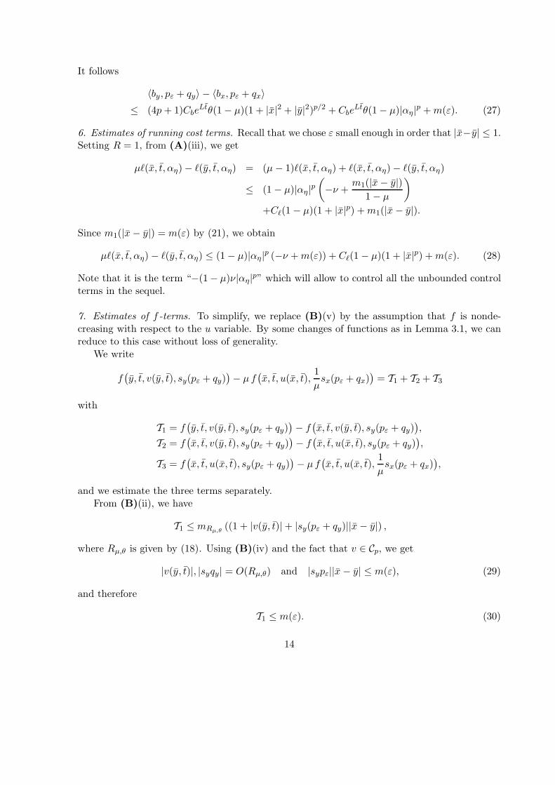
〈by, pε + qy〉 − 〈bx, pε + qx〉≤ (4p + 1)Cbe

Ltθ(1 − µ)(1 + |x|2 + |y|2)p/2 + CbeLtθ(1 − µ)|αη |p +m(ε). (27)

6. Estimates of running cost terms. Recall that we chose ε small enough in order that |x−y| ≤ 1.Setting R = 1, from (A)(iii), we get

µℓ(x, t, αη) − ℓ(y, t, αη) = (µ− 1)ℓ(x, t, αη) + ℓ(x, t, αη) − ℓ(y, t, αη)

≤ (1 − µ)|αη |p(

−ν +m1(|x− y|)

1 − µ

)

+Cℓ(1 − µ)(1 + |x|p) +m1(|x− y|).

Since m1(|x− y|) = m(ε) by (21), we obtain

µℓ(x, t, αη) − ℓ(y, t, αη) ≤ (1 − µ)|αη |p (−ν +m(ε)) + Cℓ(1 − µ)(1 + |x|p) +m(ε). (28)

Note that it is the term “−(1− µ)ν|αη|p” which will allow to control all the unbounded controlterms in the sequel.

7. Estimates of f -terms. To simplify, we replace (B)(v) by the assumption that f is nonde-creasing with respect to the u variable. By some changes of functions as in Lemma 3.1, we canreduce to this case without loss of generality.

We write

f(

y, t, v(y, t), sy(pε + qy))

− µ f(

x, t, u(x, t),1

µsx(pε + qx)

)

= T1 + T2 + T3

with

T1 = f(

y, t, v(y, t), sy(pε + qy))

− f(

x, t, v(y, t), sy(pε + qy))

,

T2 = f(

x, t, v(y, t), sy(pε + qy))

− f(

x, t, u(x, t), sy(pε + qy))

,

T3 = f(

x, t, u(x, t), sy(pε + qy))

− µ f(

x, t, u(x, t),1

µsx(pε + qx)

)

,

and we estimate the three terms separately.From (B)(ii), we have

T1 ≤ mRµ,θ((1 + |v(y, t)| + |sy(pε + qy)||x− y|) ,

where Rµ,θ is given by (18). Using (B)(iv) and the fact that v ∈ Cp, we get

|v(y, t)|, |syqy| = O(Rµ,θ) and |sypε||x− y| ≤ m(ε), (29)

and therefore

T1 ≤ m(ε). (30)

14

To deal with T2, we first note that

µu(x, t) − v(y, t) ≥ Φ(x, y, t)

≥ Φ(x, x, t)

≥ µu(x, t) − v(y, t) − eLtθ(1 − µ)(1 + 2|x|2)p/2 − ρt.

Since u(x, t) > v(y, t) by (17), if we take µ close enough to 1 and ρ, θ close enough to 0, weobtain that

µu(x, t) ≥ v(x, t).

From (B)(v) (monotonicity of f in u), it follows that

T2 ≤ f(

x, t, v(y, t), sy(pε + qy))

− f(

x, t, µu(y, t), sy(pε + qy))

+f(

x, t, µu(y, t), sy(pε + qy))

− f(

x, t, u(y, t), sy(pε + qy))

≤ (1 − µ)|u(x, t)|≤ Cu(1 − µ)(1 + |x|2)p/2, (31)

since u ∈ Cp.To estimate T3, we first recall the following convex inequality. If Ψ : IRN → IR is convex and

0 < µ < 1, then, for all ξ, ζ ∈ IRN , we have

−µΨ(ξ) + Ψ(ζ) ≤ (1 − µ)Ψ

(

µξ − ζ

µ− 1

)

. (32)

By (B)(iii) (convexity of f with respect to the gradient variable), for all z1, z2 ∈ IRN , we obtain

f(x, t, u, z1) − µ f

(

x, t, u,z2µ

)

≤ (1 − µ) f

(

x, t, u,z1 − z21 − µ

)

.

Therefore

T3 ≤ (1 − µ) f

(

x, t, u(x, t),1

1 − µ(sy(pε + qy) − sx(pε + qx))

)

≤ Cf (1 − µ)(

1 + |x|p + |u(x, t)| +∣

∣

∣

∣

sy(pε + qy) − sx(pε + qx)

1 − µ

∣

∣

∣

∣

p′)

(33)

by (B)(i). But

sy(pε + qy) − sx(pε + qx) = (sy − sx)pε + (sy − sx)qy + sx(qy − qx).

Hence for some C > 0 depending only on p (which may change during the computation), wehave

∣

∣

∣

∣

sy(pε + qy) − sx(pε + qx)

1 − µ

∣

∣

∣

∣

p′

≤ CCp′s

(1 − µ)p′

(

(|x− y||pε|)p′

+ (|x− y||qy|)p′

+ |qx − qy|p′

)

≤ ep′Ltm(ε) + CCp′

s ep′Ltθp′(1 + |x|2 + |y|2)p/2,

15

by using (29). Finally, since u ∈ Cp, we get from (33)

T3 ≤ (1 − µ)Cf (1 + Cu + CCp′s e

p′Ltθp′)(1 + |x|2 + |y|2)p/2 + ep′Ltm(ε). (34)

8. End of the case t > 0, choice of the various parameters. By plugging estimates (26), (27),(28), (30), (31) and (34) in (25), we get

LeLtθ(1−µ)(1 + |x|2 + |y|2)p/2 + ρ ≤(

C1eLtθ +C2 + C3e

p′Ltθp′)

(1−µ)(1 + |x|2 + |y|2)p/2

+(

−ν + θeLt(C4 +m(ε)))

(1−µ)|αη |p

+(1 + ep′Lt)m(ε) +m(/ε4) + η, (35)

where

C1 = 4(p − 1)2C2σ + 4(p + 1)Cb, C2 = Cℓ + Cu + Cf (1 + Cu),

C3 = CfCCp′s , C4 = 4(p− 1)C2

σ + Cb,

are positive constants which depend only on the given datas of the problem.Now we choose the different parameters in order to have a contradiction in the above in-

equality. We first assume that the final time T such that

T = 1/L > 0

(we will recover the result on any interval [0, T ] by a step-by-step argument). The main difficultyin the above estimate is to deal with the term in |αη |p since the control αη is unbounded. Takingθ > 0 such that

θe1(C4 + 1) ≤ ν

2,

we obtain that the coefficient in front of |αη|p is negative (we can assume that ε is small enoughin order to have m(ε) ≤ 1). Then we fix

L > C1 +C2

θ+ C3e

p′−1θp′−1 and η <ρ

2. (36)

Therefore (35) implies

ρ

2≤ (1 + ep

′

)m(ε) +m(/ε4).

Sending first → 0, we obtain a contradiction for small ε. In conclusion, up to a suitable choiceof the parameters θ, L, η, the claim of the Step 3 is proved if T ≤ 1/L.

9. Case when t = 0. We have just proved that there is a subsequence εn such that t = 0.Therefore for n large enough, for all (x, t) ∈ IRN × [0, T ], T ≤ 1/L, we have

µu(x, t) − v(x, t) − θ(1 − µ)eLt(1 + 2|x|2)p/2 − ρt

≤ µu(x, 0) − v(y, 0) − θ(1 − µ)(1 + |x|2 + |y|2)p/2 − |x− y|2ε2n

≤ (1 − µ)(|u(x, 0)| − θ(1 + |x|2)p/2) + u(x, 0) − v(y, 0)

≤ (1 − µ)Mθ + u(x, 0) − v(y, 0)

16

where Mθ is given by (13) since u ∈ Cp. Since u− v is upper-semicontinuous, from (19), we get

lim supεn→0

u(x, 0) − v(y, 0) ≤ u(x0, 0) − v(x0, 0) ≤ 0,

using that u(x0, 0) ≤ ψ(x0) ≤ v(x0, 0). It follows

µu(x, t) − v(x, t) − θ(1 − µ)eLt(1 + 2|x|2)p/2 − ρt ≤ (1 − µ)Mθ.

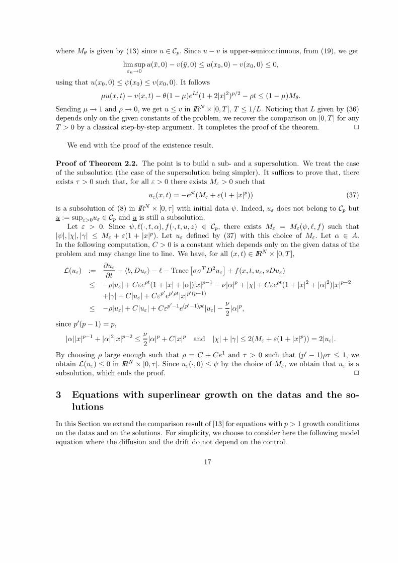
Sending µ→ 1 and ρ→ 0, we get u ≤ v in IRN × [0, T ], T ≤ 1/L. Noticing that L given by (36)depends only on the given constants of the problem, we recover the comparison on [0, T ] for anyT > 0 by a classical step-by-step argument. It completes the proof of the theorem. 2

We end with the proof of the existence result.

Proof of Theorem 2.2. The point is to build a sub- and a supersolution. We treat the caseof the subsolution (the case of the supersolution being simpler). It suffices to prove that, thereexists τ > 0 such that, for all ε > 0 there exists Mε > 0 such that

uε(x, t) = −eρt(Mε + ε(1 + |x|p)) (37)

is a subsolution of (8) in IRN × [0, τ ] with initial data ψ. Indeed, uε does not belong to Cp butu := supε>0uε ∈ Cp and u is still a subsolution.

Let ε > 0. Since ψ, ℓ(·, t, α), f(·, t, u, z) ∈ Cp, there exists Mε = Mε(ψ, ℓ, f) such that|ψ|, |χ|, |γ| ≤ Mε + ε(1 + |x|p). Let uε defined by (37) with this choice of Mε. Let α ∈ A.In the following computation, C > 0 is a constant which depends only on the given datas of theproblem and may change line to line. We have, for all (x, t) ∈ IRN × [0, T ],

L(uε) :=∂uε

∂t− 〈b,Duε〉 − ℓ− Trace

[

σσTD2uε

]

+ f(x, t, uε, sDuε)

≤ −ρ|uε| + Cεeρt(1 + |x| + |α|)|x|p−1 − ν|α|p + |χ| + Cεeρt(1 + |x|2 + |α|2)|x|p−2

+|γ| + C|uε| + Cεp′

ep′ρt|x|p′(p−1)

≤ −ρ|uε| + C|uε| + Cεp′−1e(p

′−1)ρt|uε| −ν

2|α|p,

since p′(p − 1) = p,

|α||x|p−1 + |α|2|x|p−2 ≤ ν

2|α|p + C|x|p and |χ| + |γ| ≤ 2(Mε + ε(1 + |x|p)) = 2|uε|.

By choosing ρ large enough such that ρ = C + Ce1 and τ > 0 such that (p′ − 1)ρτ ≤ 1, weobtain L(uε) ≤ 0 in IRN × [0, τ ]. Since uε(·, 0) ≤ ψ by the choice of Mε, we obtain that uε is asubsolution, which ends the proof. 2

3 Equations with superlinear growth on the datas and the so-

lutions

In this Section we extend the comparison result of [13] for equations with p > 1 growth conditionson the datas and on the solutions. For simplicity, we choose to consider here the following modelequation where the diffusion and the drift do not depend on the control.

17

∂u

∂t− Trace(σσTD2u) + 〈b,Du〉 + f(x, t, u, sDu) = 0 in IRN × [0, T ],

u(x, 0) = ψ(x) in IRN .(38)

The hypothesis on the data are the following:

(C) (Asssumptions on the diffusion and the drift)

(i) b ∈ C(IRN × [0, T ]; IRN ) and there exists Cb > 0 such that, for all x, y ∈ IRN , t ∈ [0, T ],

|b(x, t) − b(y, t)| ≤ Cb|x− y|,|b(x, t)| ≤ Cb(1 + |x|) ;

(ii) σ ∈ C(IRN × [0, T ];MN,M (IR)) is Lipschitz continuous with respect to x (uniformly in t),namely, there exists Cσ > 0 such that, for all x, y ∈ IRN and t ∈ [0, T ],

|σ(x, t) − σ(y, t)| ≤ Cσ|x− y|.

Note that σ satisfies, for every x ∈ IRN , t ∈ [0, T ],

|σ(x, t)| ≤ Cσ(1 + |x|).

We are able to consider functions which are in a larger class than in Section 2. We say thata function u : IRN × [0, T ] → IR is in the class Cp if for some C > 0 we have

|u(x, t)| ≤ C(1 + |x|p), for all (x, t) ∈ IRN × [0, T ].

The main result of this Section if the following

Theorem 3.1 Assume that σ and b satisfy (C), that f satisfies (B) and that ψ ∈ Cp. Letu ∈ USC(IRN × [0, T ]) be a viscosity subsolution of (38) and v ∈ LSC(IRN × [0, T ]) be aviscosity supersolution of (38). Suppose that U and V are in the class Cp and satisfy u(x, 0) ≤ψ(x) ≤ v(x, 0). Then u ≤ v in IRN × [0, T ].

Before giving the proof of the theorem, we state an existence result and provide some exam-ples. As observed in Section 2, we can prove the existence of solutions of (8) (at least for smalltime) as soon as we are able to build sub- and supersolutions in the class Cp. In Example 3.4,we see that solutions may not exist for all time.

Theorem 3.2 Assume (B)–(C). If K, ρ > 0 are large enough, then u(x, t) = Keρt(1 + |x|2)p/2

is a viscosity supersolution of (38) in IRN × [0, T ] and there exists 0 < τ ≤ T such that u(x, t) =−Keρt(1 + |x|2)p/2 is a viscosity subsolution of (38) in IRN × [0, τ ]. In consequence, for allψ ∈ Cp, there exists a unique continuous viscosity solution of (38) in IRN × [0, τ ] in Cp.

The proof is very close to the one of [13, Lemma 2.1], thus we omit it. Let us give someexamples of Equations for which Theorem 3.1 applies and some examples.

18

Example 3.1 The typical (simple) case we have in mind is

ut − ∆u+ |Du|p′ = −f(x, t) in IRN × [0, T ], (39)

where f satisfies (B). Note that (39) can be written

ut − ∆u+ p supα∈IRN

〈α,Du〉 − |α|p′

p′ + f(x, t) = 0

and therefore is on the form (8). The stationary version of this equation was studied in Alvarez [1]under more restrictive assumptions on the datas and the growth of the solution. More precisely,he assumed conditions like (12) and (14).

Example 3.2 Equation (8) typically appears in the study of BSDEs where s(x, t) = σ(x, t).In [9], Briand and Hu proved that u given by (7) is a viscosity solution of (8) for 1 ≤ p < 2.Theorem 3.1 proves this solution is unique. We are able to deal with any p > 1 but we had toimpose the regularity condition (B)(ii) on x for f, which is not needed for the BDSEs.

Example 3.3 As far as the coefficient f is concerned, a typical case we have in mind is

f(x, t, u, z) = g(x, t, u) + |z|p′ ,

with continuous g satisfying (B)(i),(ii) and (v). It leads to nonlinearities like “g(x, t, u) +|s(x, t)Du|p′” in the equation. Note that the power-p′ term depends on x via s(x, t). Thisdependence brings an additional difficulty, see Lemma 3.2.

Example 3.4 (Deterministic Control Problem) Consider the control problem (in dimen-sion 1 for sake of simplicity)

dXs = αs ds, s ∈ [t, T ], 0 ≤ t ≤ T,Xt = x ∈ IR,

where the control α ∈ At := Lp([t, T ]; IR) and the value function is given by

V (x, t) = infα∈At

∫ T

t(|αs|pp

+ ρ|Xs|p) ds− |XT |p for some ρ > 0.

The Hamilton-Jacobi equation formally associated to this problem is

−wt + 1p′ |wx|p

′

= ρ|x|p in IR× (0, T ),

w(x, T ) = −|x|p in IR.

Looking for a solution w under the form w(x, t) = ϕ(t)|x|p, we obtain that ϕ is a solution of thedifferential equation

−ϕ′ +|ϕ|p′

p′= ρ in (0, T ), ϕ(T ) = −1.

19

We get∫ ϕ(t)

−1

p′

|y|p′ − ρp′dy = t− T.

One can check that if 0 < ρp′ < 1 and T >∫ −1−∞

p′

|y|p′−ρp′dy, then there is τ ∈ (0, T ) such that

the solution blows up at t = τ.

Let us turn to the proof of the comparison theorem.

Proof of Theorem 3.1. To avoid a lot of technicality, we start the proof with several lemmascollecting the main intermediate results. The proofs of the lemmas are postponed at the end ofthe section and can be skipped at first reading.

Lemma 3.1 (Change of functions)Let u = e−Ltu+h(x) where h(x) = C(1+|x|p) for some constants C,L > 0. Then u is a viscositysolution of

ut − Trace(σ(x, t)σ(x, t)TD2u) + 〈b(x, t),Du〉+f(x, t, u− h, s(x, t)(Du −Dh)) = 0 in IRN × (0, T ],

u(x, 0) = ψ(x) + h(x) for all x ∈ IRN ,

(40)

with, for all (x, t, v, z) ∈ IRN × [0, T ] × IRN ,

f(x, t, v, z) = Lv + g(x, t) + e−Ltf(

x, t, eLtv, eLtz)

, (41)

where

g(x, t) = Trace(σ(x, t)σ(x, t)TD2h(x)) − 〈b(x, t),Dh(x)〉. (42)

Moreover,

f(x, t, v, z) − f(x, t, v′, z) ≤ (C − L)(v′ − v) if v ≤ v′. (43)

In the sequel, since u, v, ψ ∈ Cp, we can choose C > 0 such that

|u|, |v|, |ψ| ≤ C

2(1 + |x|p). (44)

In this case, note that

ψ(x) + h(x) = ψ(x) + C(1 + |x|p) ≥ 0

and the initial data is nonnegative in (40).Moreover, we take

L > C and L > 4p(p − 1)NC2σ + 4pCb + 10C (45)

(the constants Cσ, Cb and C appear in (B)). The first condition ensures that the right-handside of (43) is nonpositive (i.e. v 7→ f(x, t, v, z) is nondecreasing). The second condition appearsnaturally in the proof of the following lemma.

20

Lemma 3.2 (A kind of linearization procedure)Let C,L > 0 be such that (44) and (45) hold. Let 0 < µ < 1 and set w = µu− v. Then w is aviscosity subsolution of the variational inequality

min w,L[w] ≤ 0 in IRn × (0, T ),w(·, 0) ≤ 0 in IRn,

(46)

where

L[w] :=∂w

∂t− Trace[σ(x, t)σT (x, t)D2w] − Cb(1 + |x|)|Dw| + L

4(1 − µ)h(x, t)

−(1 − µ)e−Ltf

(

x, t, 0, eLts(x, t)(Dw

µ− 1−Dh(x))

)

(47)

and h is defined in Lemma 3.1.

Lemma 3.3 (An auxiliary parabolic problem)Consider, for any R > 0, the parabolic problem

ϕt − r2ϕrr − rϕr = 0 in [0,+∞) × (0, T ],ϕ(r, 0) = max0, r −R in [0,+∞).

(48)

Then (48) has a unique solution ϕR ∈ C([0,+∞) × [0, T ]) ∩ C∞([0,+∞) × (0, T ]) such that,for all t ∈ (0, T ], ϕR(·, t) is positive, nondecreasing and convex in [0,+∞). Moreover, for every(r, t) ∈ [0,+∞) × (0, T ],

ϕR(r, t) ≥ max0, r −R, 0 ≤ ∂ϕR

∂r(r, t) ≤ eT and ϕR(r, t) −→

R→+∞0. (49)

For the proof of Lemma 3.3 we refer the reader to [13].

Lemma 3.4 (Construction of a smooth strict supersolution)Let Φ(x, t) = ϕR(h(x), Ct) where ϕR is given by Lemma 3.3, h(x) = C(1+ |x|p), C satisfies (44)and C > 0. Then, for C and L = L(µ) large enough, we have

L[Φ(x, t)] > 0 for all (x, t) ∈ IRN × (0, 1/L], (50)

where L is defined by (47).

Now, we continue the proof of Theorem 3.1. Consider

maxIRN×[0,1/L]

w − Φ, (51)

where w is given by Lemma 3.2 and Φ is the function built in Lemma 3.4. From (49), for |x|large enough, we have Φ(x, t) ≥ C(1 + |x|p)−R. Since w ≤ (µ+ 1)C(1 + |x|p)/2, it follows thatthe maximum (51) is achieved at a point (x, t) ∈ IRN × [0, 1/L]. We can assume that w(x, t) > 0otherwise, arguing as in (52)-(53), we prove w ≤ 0 in IRN × [0, 1/L] and the conclusion follows.

21

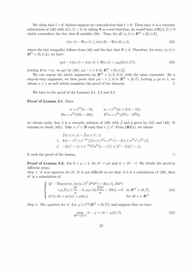
We claim that t = 0. Indeed suppose by contradiction that t > 0. Then since w is a viscositysubsolution of (46) with w(x, t) > 0, by taking Φ as a test-function, we would have L[Φ](x, t) ≤ 0which contradicts the fact that Φ satisfies (50) . Thus, for all (x, t) ∈ IRN × [0, 1/L],

w(x, t) − Φ(x, t) ≤ w(x, 0) − Φ(x, 0) ≤ 0, (52)

where the last inequality follows from (46) and the fact that Φ ≥ 0. Therefore, for every (x, t) ∈IRN × [0, 1/L], we have

(µu− v)(x, t) = w(x, t) ≤ Φ(x, t) = ϕR(h(x), Ct). (53)

Letting R to +∞, we get by (49), µu− v ≤ 0 in IRN × [0, 1/L].We can repeat the above arguments on IRN × [1/L, 2/L] with the same constants. By a

step-by-step argument, we then prove that µu − v ≤ 0 in IRN × [0, T ]. Letting µ go to 1, weobtain u ≤ v as well which completes the proof of the theorem. 2

We turn to the proof of the Lemmas 3.1, 3.2 and 3.4.

Proof of Lemma 3.1. Since

u = eLt(u− h), ut = eLt(ut + L(u− h)),

Du = eLt(Du−Dh), D2u = eLt(D2u−D2h),

we obtain easily that u is a viscosity solution of (40) with f and g given by (41) and (42). Itremains to check (43)). Take v, v′ ∈ IR such that v ≤ v′. From (B)(v), we obtain

f(x, t, v, z) − f(x, t, v′, z)

≤ L(v − v′) + e−Lt(

f(x, t, eLtv, eLtz) − f(x, t, eLtv′, eLtz))

≤ −L(v′ − v) + e−LtC|eLt(v − v′)| ≤ (C − L)(v′ − v).

It ends the proof of the lemma. 2

Proof of Lemma 3.2. For 0 < µ < 1, let uµ = µu and w = uµ − v. We divide the proof indifferent steps.Step 1. A new equation for uµ. It is not difficult to see that, if u is a subsolution of (40), thenuµ is a subsolution of

uµt − Trace(σ(x, t)σ(x, t)TD2uµ) + 〈b(x, t),Duµ〉

+µ f(x, t,uµ

µ− h, s(x, t)(

Duµ

µ−Dh)) = 0 in IRN × (0, T ],

uµ(x, 0) = µψ(x) + µh(x) for all x ∈ IRN .

(54)

Step 2. The equation for w. Let ϕ ∈ C2(IRN × [0, T ]) and suppose that we have

maxIRN×[0,T ]

w − ϕ = (w − ϕ)(x, t). (55)

22

We distinguish 3 cases.At first, if the maximum is achieved for t = 0, then, writing that uµ is a subsolution of (54)

and v a supersolution of (40) at t = 0 we obtain uµ(x, 0) ≤ µψ(x) + µh(x) and v(x, 0) ≥ψ(x) + h(x). It follows that

w(x, 0) ≤ (µ− 1)(ψ(x) + h(x)) = (µ− 1)(ψ(x) + C(1 + |x|p)) ≤ 0

by (44). Therefore w satisfies (46) at (x, 0).Secondly, we suppose that t > 0 and w(x, t) ≤ 0. Again, w satisfies (46) at (x, t).From now on, we consider the last and most difficult case when

t > 0 and w(x, t) > 0. (56)

Step 3. Viscosity inequalities for uµ and v. This step is classical in viscosity theory. We canassume that the maximum in (55) at (x, t) is strict in the some ball B(x, r)× [t− r, t+ r] (see [6]or [3]). Let

Θ(x, y, t) = ϕ(x, t) +|x− y|2ε2

and considerMε := max

x,y∈B(x,r), t∈[t−r,t+r]uµ(x, t) − v(y, t) − Θ(x, y, t).

This maximum is achieved at a point (xε, yε, tε) and, since the maximum is strict, we know that

xε, yε → x,|xε − yε|2

ε2→ 0, (57)

andMε = uµ(xε, tε) − v(yε, tε) − Θ(xε, yε, tε) −→(w − ϕ)(x, t) as ε→ 0.

It means that, at the limit ε → 0, we obtain some information on w − ϕ at (x, t) which willprovide the new equation for w. From (56), for ε small enough, we have

uµ(xε, tε) − v(yε, tε) > 0. (58)

We can take Θ as a test-function to use the fact that uµ is a subsolution of (54) and v asupersolution of (40). Indeed (x, t) ∈ B(x, r) × [t − r, t + r] 7→ uµ(x, t) − v(yε, t) − Θ(x, yε, t)achieves its maximum at (xε, tε) and (y, t) ∈ B(x, r)×[t−r, t+r] 7→ −uµ(xε, t)+v(y, t)+Θ(xε, y, t)achieves its minimum at (yε, tε). Thus, by Theorem 8.3 in the User’s guide [11], for every ρ > 0,there exist a1, a2 ∈ IR and X,Y ∈ SN such that

(a1,DxΘ(xε, yε, tε),X) ∈ P2,+(uµ)(xε, tε), (a2,−DyΘ(xε, yε, tε), Y ) ∈ P2,−(v)(yε, tε),

a1 − a2 = Θt(xε, yε, tε) = ϕt(xε, tε) and

−(1

ρ+ |M |)I ≤

(

X 00 −Y

)

≤M + ρM2 where M = D2Θ(xε, yε, tε). (59)

23

Setting pε = 2xε − yε

ε2, we have

DxΘ(xε, yε, tε) = pε +Dϕ(xε, tε) and DyΘ(xε, yε, tε) = −pε,

and

M =

(

D2ϕ(xε, tε) + 2I/ε2 −2I/ε2

−2I/ε2 2I/ε2

)

.

Thus, from (59), it follows

〈Xp, p〉 − 〈Y q, q〉 ≤ 〈D2ϕ(xε, tε)p, p〉 +2

ε2|p− q|2 +m

( ρ

ε4

)

, (60)

where m is a modulus of continuity which is independent of ρ and ε. In the sequel, m will alwaysdenote a generic modulus of continuity independent of ρ and ε.

Writing the subsolution viscosity inequality for uµ and the supersolution inequality for v bymeans of the semi-jets and subtracting the inequalities, we obtain

ϕt(xε, tε)

−Trace[

σ(xε, tε)σT (xε, tε)X

]

+ Trace[

σ(yε, tε)σT (yε, tε)Y

]

−〈b(xε, tε), pε +Dϕ(xε, tε)〉 + 〈b(yε, tε), pε〉

+µf

(

xε, tε,uµ(xε, tε)

µ− h(xε), s(xε, tε)(

pε +Dϕ(xε, tε)

µ−Dh(xε))

)

−f (yε, tε, v(yε, tε) − h(yε), s(yε, tε)(pε −Dh(yε)))

≤ 0 (61)

Now, we derive some estimates for the various terms appearing in (61) in order to be ableton send ε→ 0. The estimates for the σ and b terms are classical wheras those for the f termsare more involved.

For the sake of simplicity, for any function g : IRN × [0, T ] → IR, we set

g(xε, tε) = gx and g(yε, tε) = gy.

Step 4. Estimate of σ-terms. Let us denote by (ei)1≤i≤N the canonical basis of IRN . By us-ing (60), we obtain

Trace[

cxσTxX − σyσ

Ty Y]

=N∑

i=1

〈Xσxei, σxei〉 − 〈Y σyei, σyei〉

≤ Trace[

σxσTxD

2ϕ(xε, tε)]

+2

ε2|σx − σy|2 +m

( ρ

ε4

)

≤ Trace[

σxσTxD

2ϕ(xε, tε)]

+ 2C2σ,r

|xε − yε|2ε2

+m( ρ

ε4

)

≤ Trace[

σσT (x, t)D2ϕ(x, t)]

+m(ε) +m( ρ

ε4

)

, (62)

24

where Cσ,r is a Lipschitz constant for σ in B(x, r) and we used that σ is continuous, ϕ is C2

and (57).Step 5. Estimate of b-terms. From (C), if Cb,r is the Lipschitz constant of b inB(x, r)×[t−r, t+r],then we have

〈b(xε, tε) − b(yε, tε), pε〉 ≤ Cb,r|xε − yε||pε| ≤ 2Cb,r|xε − yε|2

ε2= m(ε)

and

〈b(xε, tε),Dϕ(xε, tε)〉 ≤ Cb(1 + |xε|)|Dϕ(xε, tε)|.

It follows

〈b(xε, tε), pε +Dϕ(xε, tε)〉 − 〈b(yε, tε), pε〉 ≤ Cb(1 + |x|)|Dϕ(x, t)| +m(ε) (63)

Step 6. Estimate of f-terms. We write

−µf(

xε, tε,uµ(xε, tε)

µ− hx, sx(

pε +Dϕ(xε, tε)

µ−Dhx)

)

+f (yε, tε, v(yε, tε) − hy, sy(pε −Dhy))

= T1 + T2 + T3

where

T1 = −µf(

xε, tε,uµ(xε, tε)

µ− hx, sx(

pε +Dϕ(xε, tε)

µ−Dhx)

)

+µf

(

xε, tε, v(yε, tε) − hy, sx(pε +Dϕ(xε, tε)

µ−Dhx)

)

,

T2 = −µf(

xε, tε, v(yε, tε) − hy, sx(pε +Dϕ(xε, tε)

µ−Dhx)

)

+µf

(

yε, tε, v(yε, tε) − hy, sx(pε +Dϕ(xε, tε)

µ−Dhx)

)

,

T3 = −µf(

yε, tε, v(yε, tε) − hy, sx(pε +Dϕ(xε, tε)

µ−Dhx)

)

+f (yε, tε, v(yε, tε) − hy, sy(pε −Dhy)) .

We estimate T1. From (58), we have

u(xε, tε) =uµ(xε, tε)

µ> v(yε, tε) + (1 − µ)u(xε, tε).

25

Using (43) (the monotonicity in u of f) and then (B)(v) (Lipschitz continuity in u of f), we get

f

(

xε, tε,uµ(xε, tε)

µ− hx, sx(

pε +Dϕ(xε, tε)

µ−Dhx)

)

≥ f

(

xε, tε, v(yε, tε) + (1 − µ)u(xε, tε) − hx, sx(pε +Dϕ(xε, tε)

µ−Dhx)

)

≥ f

(

xε, tε, v(yε, tε) + hy, sx(pε +Dϕ(xε, tε)

µ−Dhx)

)

−C(1 − µ)|u(xε, tε)| − C|hx − hy|.

Since h is continuous, we have C|hx − hy| = m(ε). By (44) and since xε → x, we obtain

C(1 − µ)|u(xε, tε)| ≤ CC(1 − µ)(1 + |xε|p) = C(1 − µ)h(x) +m(ε).

Therefore

T1 ≤ C(1 − µ)h(x) +m(ε). (64)

The estimate of T2 relies on (B)(ii). Setting Qε = eLtεsx(pε+Dϕ(xε,tε)µ −Dhx) and recalling

that r is defined at the beginning of Step 3, we have

|T2| ≤ µ|g(xε, tε) − g(yε, tε)|+µe−Ltε |f(xε, tε, e

Ltε(v(yε, tε) − hy), Qε) − f(yε, tε, e−Ltε(v(yε, tε) − hy), Qε)|

≤ µ|g(xε, tε) − g(yε, tε)|+µe−Ltε m2r

(

(1 + |eLtε(v(yε, tε) − hy)| + |Qε|)|xε − yε|)

≤ m(ε), (65)

since g is continuous, |xε − yε| = m(ε) and pε|xε − yε| = |xε − yε|2/ε2 = m(ε) by (57).Let us turn to the estimate of T3. We have

T3 = L(1 − µ)(v(yε, tε) − hy) + (1 − µ)g(yε, tε)

−µe−Ltεf

(

yε, tε, eLtε(v(yε, tε) − hy), e

Ltεsx(pε +Dϕ(xε, tε)

µ−Dhx)

)

+e−Ltεf(

yε, tε, eLtε(v(yε, tε) − hy), e

Ltεsy(pε −Dhy))

.

At first, from (44), we have

L(1 − µ)(v(yε, tε) − hy) ≤ −L(1 − µ)

2h(x) +m(ε).

Using (C) (see (68) for the details), a straightforward computation gives an estimate for thecontinuous function g:

|g(yε, tε)| ≤ (p(p− 1)NC2σ + pCb)h(x) +m(ε).

26

Now we estimate the f -terms. From (B)(iii) (convexity of f with respect to the gradientvariable), we can apply (32) to obtain

−µe−Ltεf

(

yε, tε, eLtε(v(yε, tε) − hy), e

Ltεsx(pε +Dϕ(xε, tε)

µ−Dhx)

)

+e−Ltεf(

yε, tε, eLtε(v(yε, tε) − hy), e

Ltεsy(pε −Dhy))

≤ (1 − µ)e−Ltεf(

yε, tε, eLtε(v(yε, tε) − hy), Qε

)

,

where

Qε =eLtε

µ− 1((sx − sy)pε + sxDϕ(xε, tε) + syDhy − µsxDhx)

= eLts(x, t)

(

Dϕ(x, t)

µ− 1−Dh(x)

)

+m(ε).

from (B)(iv) and (57). From (B)(v), (44) and the continuity of f, it follows

e−Ltεf(

yε, tε, eLtε(v(yε, tε) − hy), Qε

)

≤ e−Ltf

(

x, t, 0, eLts(x, t)

(

Dϕ(x, t)

µ− 1−Dh(x)

))

+3C

2h(x) +m(ε).

Finally, we obtain

T3 ≤ (1 − µ)

(

−L2

+ p(p− 1)NC2σ + pCb +

3C

2

)

h(x)

+e−Ltf

(

x, t, 0, eLts(x, t)

(

Dϕ(x, t)

µ− 1−Dh(x)

))

+m(ε). (66)

Step 7. End of the proof. Combining (61), (62), (63), (64), (65) and (66), setting L > 4p(p −1)NC2

σ + 4pCb + 10C and sending ρ→ 0 and then ε→ 0, we get

ϕt(x, t) − Trace[

σσT (x, t)D2ϕ(x, t)]

− Cb(1 + |x|)|Dϕ(x, t)| + L

4(1 − µ)h(x)

−(1 − µ)e−Ltf

(

x, t, 0, eLts(x, t)

(

Dϕ(x, t)

µ− 1−Dh(x)

))

≤ 0,

which is exactly the new equation for w in the case (56). It completes the proof of the lemma. 2

Proof of Lemma 3.4. For simplicity, we fix R and set ϕ = ϕR for simplicity. Therefore ϕr

denotes the derivative of ϕ wrt the space variable. We compute

Φt = Cϕt, DΦ = ϕrDh,

D2Φ = ϕrD2h+ ϕrrDh⊗Dh,

27

with

h = C(1 + |x|p), Dh = pC|x|p−2x, D2h = pC(|x|p−2Id+ (p − 2)|x|p−4x⊗ x).

For all (x, t) ∈ IRN × (0, T ],

L(Φ(x, t))

= Cϕt −(

Trace(σσTD2h) + Cb(1 + |x|)|Dh|)

ϕr − Trace(σσTDh⊗Dh)ϕrr

+(1 − µ)L

4h− (1 − µ)e−Ltf

(

x, t, 0, eLts

(

ϕr

µ− 1+ 1

)

Dh

)

. (67)

Using (C)(ii) and the fact that p′(p− 1) = p, we have the following estimates:

|Dh| ≤ pC|x|p−1, |D2h| ≤ p(p− 1)C|x|p−2,

Cb(1 + |x|)|Dh| ≤ pCbh,

|Trace(σσTD2h)| ≤ p(p− 1)NC2σh,

0 ≤ Trace(σσTDh⊗Dh) ≤ C2σ(1 + |x|2)p2C

2|x|2(p−1) ≤ p2C2σh

2.

(68)

Now, the assumption (B)(i) on the growth of f plays a crucial role:

f

(

x, t, 0, eLts

(

ϕr

µ− 1+ 1

)

Dh

)

≤ Cf

(

1 + |x|p +

∣

∣

∣

∣

eLts

(

ϕr

µ− 1+ 1

)

Dh

∣

∣

∣

∣

p′)

≤ Cf

(

1

C+ pp′Cp′

s Cp′−1

eLp′t

(

eT

1 − µ+ 1

)p′)

h(x)

since ϕr ≤ eT (Lemma 3.3) and |Dh|p′ ≤ pp′Cp′−1

h(x) (because p′(p − 1) = p). It followsfrom (67),

L(Φ(x, t))

≥ Cϕt − (p(p − 1)NC2σ + pCb)ϕr − p2C2

σh2ϕrr

+(1 − µ)

(

L

4− Cf e−Lt

C− pp′Cp′

s Cp′−1

eLp′t

(

eT

1 − µ+ 1

)p′)

h(x).

We take

C > max

p(p− 1)NC2σ + pCb, p

2C2σ

,

L >4Cf

C+ 4pp′Cp′

s Cp′−1

ep′(

eT

1 − µ+ 1

)p′

+ 1 and (45) holds,

τ =1

L.

For this choice of parameters, for all (x, t) ∈ IRN × (0, τ ], we have

L(Φ(x, t)) ≥ C(

ϕt(h,Ct) − hϕr(h,Ct) − h2ϕrr(h,Ct))

+ (1 − µ)h > 0

since ϕ is a solution of (48) and h > 0. This proves the lemma. 2

28

References

[1] O. Alvarez. A quasilinear elliptic equation in RN . Proc. Roy. Soc. Edinburgh Sect. A, 126(5):911–921,1996.

[2] O. Alvarez. Bounded-from-below viscosity solutions of Hamilton-Jacobi equations. DifferentialIntegral Equations, 10(3):419–436, 1997.

[3] M. Bardi and I. Capuzzo Dolcetta. Optimal control and viscosity solutions of Hamilton-Jacobi-Bellman equations. Birkhauser Boston Inc., Boston, MA, 1997.

[4] M. Bardi and F. Da Lio. On the Bellman equation for some unbounded control problems. NoDEANonlinear Differential Equations Appl., 4(4):491–510, 1997.

[5] G. Barles. An approach of deterministic control problems with unbounded data. Ann. Inst. H.Poincare Anal. Non Lineaire, 7(4):235–258, 1990.

[6] G. Barles. Solutions de viscosite des equations de Hamilton-Jacobi. Springer-Verlag, Paris, 1994.

[7] G. Barles, S. Biton, M. Bourgoing, and O. Ley. Uniqueness results for quasilinear parabolic equationsthrough viscosity solutions’ methods. Calc. Var. Partial Differential Equations, 18(2):159–179, 2003.

[8] A. Bensoussan. Stochastic control by functional analysis methods, volume 11 of Studies in Mathe-matics and its Applications. North-Holland Publishing Co., Amsterdam, 1982.

[9] P. Briand and Y. Hu. Quadratic BSDEs with convex generators and unbounded terminal conditions.Probab. Theory Related Fields, 141(3-4):543–567, 2008.

[10] P. Cannarsa and G. Da Prato. Nonlinear optimal control with infinite horizon for distributedparameter systems and stationary Hamilton-Jacobi equations. SIAM J. Control Optim., 27(4):861–875, 1989.

[11] M. G. Crandall, H. Ishii, and P.-L. Lions. User’s guide to viscosity solutions of second order partialdifferential equations. Bull. Amer. Math. Soc. (N.S.), 27(1):1–67, 1992.

[12] M. G. Crandall and P.-L. Lions. Quadratic growth of solutions of fully nonlinear second orderequations in IRn. Differential Integral Equations, 3(4):601–616, 1990.

[13] F. Da Lio and O. Ley. Uniqueness results for second-order Bellman-Isaacs equations under quadraticgrowth assumptions and applications. SIAM J. Control Optim., 45(1):74–106, 2006.

[14] F. Da Lio and W. M. McEneaney. Finite time-horizon risk-sensitive control and the robust limitunder a quadratic growth assumption. SIAM J. Control Optim., 40(5):1628–1661 (electronic), 2002.

[15] W. H. Fleming and R. W. Rishel. Deterministic and stochastic optimal control. Springer-Verlag,Berlin, 1975. Applications of Mathematics, No. 1.

[16] W. H. Fleming and H. M. Soner. Controlled Markov processes and viscosity solutions. Springer-Verlag, New York, 1993.

[17] H. Ishii. Perron’s method for Hamilton-Jacobi equations. Duke Math. J., 55(2):369–384, 1987.

[18] H. Ishii. Comparison results for Hamilton-Jacobi equations without growth condition on solutionsfrom above. Appl. Anal., 67(3-4):357–372, 1997.

[19] K. Ito. Existence of solutions to Hamilton-Jacobi-Bellman equation under quadratic growth condi-tions. J. Differential Equations, 176:1–28, 2001.

[20] M. Kobylanski. Backward stochastic differential equations and partial differential equations withquadratic growth. Ann. Probab., 28(2):558–602, 2000.

29

[21] N. V. Krylov. Stochastic linear controlled systems with quadratic cost revisited. In Stochastics infinite and infinite dimensions, Trends Math., pages 207–232. Birkhauser Boston, Boston, MA, 2001.

[22] B. Øksendal. Stochastic differential equations. Universitext. Springer-Verlag, Berlin, fifth edition,1998. An introduction with applications.

[23] E. Pardoux and S. G. Peng. Adapted solution of a backward stochastic differential equation. SystemsControl Lett., 14(1):55–61, 1990.

[24] F. Rampazzo and C. Sartori. Hamilton-Jacobi-Bellman equations with fast gradient-dependence.Indiana Univ. Math. J., 49(3):1043–1077, 2000.

[25] J. Yong and Xun Y. Zhou. Stochastic controls, volume 43 of Applications of Mathematics. Springer-Verlag, New York, 1999. Hamiltonian systems and HJB equations.

30