unicorn on rainbow: a universal commonsense reasoning

UNICORN on RAINBOW:A Universal Commonsense Reasoning Model on a New Multitask Benchmark

Nicholas Lourie♠ Ronan Le Bras♠ Chandra Bhagavatula♠ Yejin Choi ♥♠

♠ Allen Institute for AI, WA, USA♥ Paul G. Allen School of Computer Science & Engineering, WA, USA

Abstract

Commonsense AI has long been seen as a near impossiblegoal—until recently. Now, research interest has sharply in-creased with an influx of new benchmarks and models.We propose two new ways to evaluate commonsense models,emphasizing their generality on new tasks and building ondiverse, recently introduced benchmarks. First, we propose anew multitask benchmark, RAINBOW, to promote research oncommonsense models that generalize well over multiple tasksand datasets. Second, we propose a novel evaluation, the costequivalent curve, that sheds new insight on how the choiceof source datasets, pretrained language models, and transferlearning methods impacts performance and data efficiency.We perform extensive experiments—over 200 experimentsencompassing 4800 models—and report multiple valuableand sometimes surprising findings, e.g., that transfer almostalways leads to better or equivalent performance if follow-ing a particular recipe, that QA-based commonsense datasetstransfer well with each other, while commonsense knowledgegraphs do not, and that perhaps counter-intuitively, largermodels benefit more from transfer than smaller ones.Last but not least, we introduce a new universal com-monsense reasoning model, UNICORN, that establishes newstate-of-the-art performance across 8 popular commonsensebenchmarks, αNLI (→87.3%), COSMOSQA (→91.8%),HELLASWAG (→93.9%), PIQA (→90.1%), SOCIALIQA(→83.2%), WINOGRANDE (→86.6%), CYCIC (→94.0%)and COMMONSENSEQA (→79.3%).

1 IntroductionIn AI’s early years, researchers sought to build machineswith common sense (McCarthy 1959); however, in the fol-lowing decades, common sense came to be viewed as a nearimpossible goal. It is only recently that we see a sudden in-crease in research interest toward commonsense AI, with aninflux of new benchmarks and models (Mostafazadeh et al.2016; Talmor et al. 2019; Sakaguchi et al. 2020).

This renewed interest in common sense is ironically en-couraged by both the great empirical strengths and limita-tions of large-scale pretrained neural language models. Onone hand, pretrained models have led to remarkable progressacross the board, often surpassing human performance on

Copyright © 2021, Association for the Advancement of ArtificialIntelligence (www.aaai.org). All rights reserved.

Figure 1: Cost equivalent curves comparing transfer learn-ing from GLUE, SUPERGLUE, and RAINBOW onto COM-MONSENSEQA. Each curve plots how much training datathe single-task baseline (the x-axis) needs compared to themultitask method (the y-axis) to achieve the same perfor-mance (shown on the top axis in accuracy). Curves belowthe diagonal line (y = x) indicate that the multitask methodneeds less training data from the target dataset than thesingle-task baseline for the same performance. Thus, lowercurves mean more successful transfer learning.

leaderboards (Radford et al. 2018; Devlin et al. 2019; Liuet al. 2019b; Raffel et al. 2019). On the other hand, pre-trained language models continue to make surprisingly sillyand nonsensical mistakes, even the recently introduced GPT-3.1 This motivates new, relatively under-explored researchavenues in commonsense knowledge and reasoning.

In pursuing commonsense AI, we can learn a great dealfrom mainstream NLP research. In particular, the introduc-tion of multitask benchmarks such as GLUE (Wang et al.2019b) and SUPERGLUE (Wang et al. 2019a) has encour-aged fundamental advances in the NLP community, acceler-ating research into models that robustly solve many tasksand datasets instead of overfitting to one in particular. Incontrast, commonsense benchmarks and models are rela-tively nascent, thus there has been no organized effort, to

1https://www.technologyreview.com/2020/08/22/1007539/gpt3-openai-language-generator-artificial-intelligence-ai-opinion/

arX

iv:2

103.

1300

9v1

[cs

.CL

] 2

4 M

ar 2

021

date, at administering a collection of diverse commonsensebenchmarks and investigating transfer learning across them.

We address exactly this need, proposing two new waysto evaluate commonsense models with a distinct emphasison their generality across tasks and domains. First, we pro-pose a new multi-task benchmark, RAINBOW, to facilitateresearch into commonsense models that generalize well overmultiple different tasks and datasets. Second, we proposea novel evaluation, the cost equivalent curve, that shedsnew insight on how different choices of source datasets, pre-trained language models, and transfer learning methods af-fect performance and data efficiency in the target dataset.

The primary motivation for cost equivalent curves is dataefficiency. The necessary condition for state-of-the-art neu-ral models to maintain top performance on any dataset isa sufficiently large amount of training data for fine-tuning.Importantly, building a dataset for a new task or a domainis an expensive feat, easily costing tens of thousands of dol-lars (Zellers et al. 2018). Therefore, we want the models togeneralize systematically across multiple datasets, instead ofrelying solely on the target dataset.

Shown in Figure 1, the cost equivalent curve aims to an-swer the following intuitive question: how much data doesa transfer learning approach save over the baseline thatdoesn’t benefit from transfer learning? We provide a moredetailed walk-through of this chart in §2. As will be seen,cost equivalent curves have distinct advantages over sim-ple evaluations at the full dataset size or classical learningcurves drawn for each method and dataset separately, as theyprovide more accurate comparative insights into data effi-ciency in the context of multitasking and transfer learning.

We leverage these new tools to reevaluate commonapproaches for intermediate-task transfer (Pruksachatkunet al. 2020). Through extensive experiments, we identifymultiple valuable and sometimes surprising findings, e.g.,that intermediate-task transfer can always lead to better orequivalent performance if following a particular recipe, thatQA-based commonsense datasets transfer well to each other,while commonsense knowledge graphs do not, and that per-haps counter-intuitively, larger models benefit much morefrom transfer learning compared to smaller ones.

In addition to the empirical insights, we also intro-duce a new universal commonsense reasoning model:UNICORN, establishing new state-of-the-art performancesacross 8 benchmarks: αNLI (87.3%) (Bhagavatula et al.2020), COSMOSQA (91.8%) (Huang et al. 2019), HEL-LASWAG (93.9%) (Zellers et al. 2019), PIQA (90.1%)(Bisk et al. 2020), SOCIALIQA (83.2%) (Sap et al. 2019b),WINOGRANDE (86.6%) (Sakaguchi et al. 2020), CY-CIC (94.0%),2 as well as the popular COMMONSENSEQAdataset (79.3%) (Talmor et al. 2019). Beyond setting recordswith the full training sets, our ablations show UNICORN alsoimproves data efficiency for all training dataset sizes.

For reproducibility, we publicly release the UNICORNmodel and code, all the experimental results, and the RAIN-BOW leaderboard at https://github.com/allenai/rainbow.

2The CYCIC dataset and leaderboard are available at https://leaderboard.allenai.org/cycic.

2 Cost Equivalent CurvesCost equivalent curves show equivalent costs between thesingle-task baseline and a new transfer-based approach. Inthis work, we define cost as the number of training examplesin the target dataset. Intuitively, we want to measure howmany examples the new approach needs to match the single-task baseline’s performance as the amount of data varies.

Figure 1 illustrates cost equivalent curves with COMMON-SENSEQA as the target dataset. The x-axis shows the num-ber of examples used by the single-task baseline, while they-axis shows the examples from the target dataset used bythe new multitask method. The curve is where they achievethe same performance. The numbers on top of the figureshow the performance corresponding to the number of base-line examples from the x-axis. For example, with 4.9k exam-ples, the baseline achieves 70% accuracy. For any number ofexamples the baseline might use, we can see how many ex-amples the new approach would require to match it. In Fig-ure 1, to match the baseline’s performance on ∼10k exam-ples, multitasking with RAINBOW requires about 5k, whilemultitasking with GLUE requires more than 10k. Thus,lower is better, with curves below the diagonal (y = x) in-dicating that the new method improves over the baseline.

The construction of cost equivalent curves makes onetechnical assumption: the relationship between performanceand cost is continuous and strictly monotonic (i.e., increas-ing or decreasing). This assumption holds empirically forparameters, compute, and data (Kaplan et al. 2020). Thus,we can safely estimate each learning curve with isotonic re-gression (Barlow et al. 1972), then construct the cost equiv-alent curve by mapping each dataset size to the baselineperformance, finding the matching performance on the newmethod’s curve, and seeing how many examples are re-quired.

Cost equivalent curves visualize how a new approach im-pacts the cost-benefit trade-off, i.e. examples required for agiven performance. This reframes the goal from pushing upperformance on a fixed-size benchmark to most efficientlysolving the problem. While we focus on data efficiency inthis work, the idea of cost equivalent curves can be appliedto other definitions of cost as well (e.g., GPU compute).

3 RAINBOWWe define RAINBOW, a suite of commonsense benchmarks,with the following datasets. To keep evaluation clean-cut,we only chose multiple-choice question-answering datasets.αNLI (Bhagavatula et al. 2020) tests abductive reasoning

in narratives. It asks models to identify the best explana-tion among several connecting a beginning and ending.

COSMOSQA (Huang et al. 2019) asks commonsense read-ing comprehension questions about everyday narratives.

HELLASWAG (Zellers et al. 2019) requires models tochoose the most plausible ending to a short context.

PIQA (Bisk et al. 2020) is a multiple-choice question an-swering benchmark for physical commonsense reasoning.

SOCIALIQA (Sap et al. 2019b) evaluates commonsensereasoning about social situations and interactions.

Figure 2: A comparison of transfer methods on RAINBOW tasks with T5-LARGE. Each plot varies the data available for onetask while using all data from the other five to generate the cost equivalent curve. Performance is measured by dev set accuracy.

TRANSFER αNLI COSMOSQA HELLASWAG PIQA SOCIALIQA WINOGRANDE

multitask 78.4 81.1 81.3 80.7 74.8 72.1fine-tune 79.2 82.6 83.1 82.2 75.2 78.2sequential 79.5 83.2 83.0 82.2 75.5 78.7none 77.8 81.9 82.8 80.2 73.8 77.0

Table 1: A comparison of transfer methods’ dev accuracy (%) on the RAINBOW tasks, using the T5-LARGE model.

WINOGRANDE (Sakaguchi et al. 2020) is a large-scalecollection of Winograd schema-inspired problems requir-ing reasoning about both social and physical interactions.

4 Empirical InsightsWe present results from our large-scale empirical study,using pretrained T5-LARGE to transfer between datasets.We’ve grouped our findings and their relevant figures aroundthe four following thematic questions.

4.1 What’s the Best Approach for Transfer?We compare three recipes for intermediate-task transfer:

(1) multitask training (Caruana 1995): training on multi-ple datasets (including the target dataset) all at once,

(2) sequential training (Pratt, Mostow, and Kamm 1991):first training on multiple datasets (excluding the target

dataset) through multitask training, and then continuingto train on the target dataset alone,

(3) multitask fine-tuning (Liu et al. 2019a): first trainingon all datasets (including the target dataset) through mul-titask training, and then continuing to fine-tune on the tar-get dataset alone.

Figure 2 compares these three methods on each of the sixRAINBOW tasks, using the other five datasets for transfer.

Finding 1: Sequential training almost always matches orbeats other approaches. Generally, sequential and mul-titask fine-tune training use fewer examples to achieve thesame performance as multitask training or the single taskbaseline.3 For some tasks (αNLI and SOCIALIQA), all three

3Equivalently, they achieve better performance for the samenumber of examples.

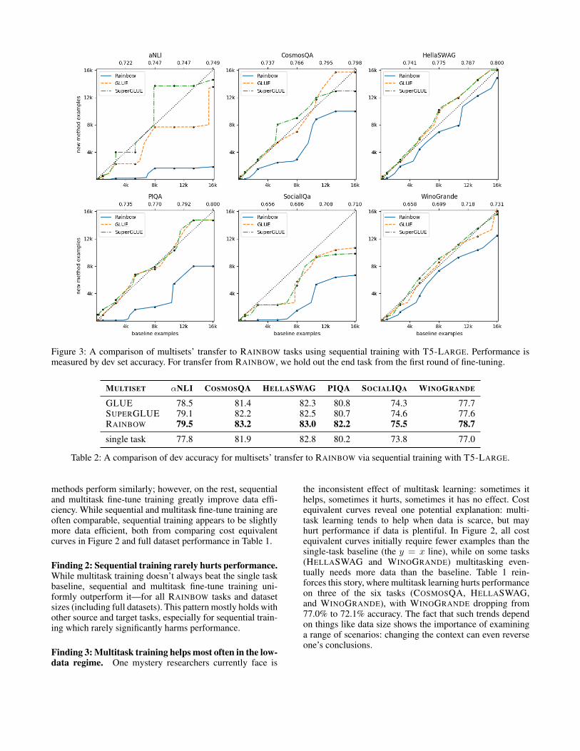
Figure 3: A comparison of multisets’ transfer to RAINBOW tasks using sequential training with T5-LARGE. Performance ismeasured by dev set accuracy. For transfer from RAINBOW, we hold out the end task from the first round of fine-tuning.

MULTISET αNLI COSMOSQA HELLASWAG PIQA SOCIALIQA WINOGRANDE

GLUE 78.5 81.4 82.3 80.8 74.3 77.7SUPERGLUE 79.1 82.2 82.5 80.7 74.6 77.6RAINBOW 79.5 83.2 83.0 82.2 75.5 78.7single task 77.8 81.9 82.8 80.2 73.8 77.0

Table 2: A comparison of dev accuracy for multisets’ transfer to RAINBOW via sequential training with T5-LARGE.

methods perform similarly; however, on the rest, sequentialand multitask fine-tune training greatly improve data effi-ciency. While sequential and multitask fine-tune training areoften comparable, sequential training appears to be slightlymore data efficient, both from comparing cost equivalentcurves in Figure 2 and full dataset performance in Table 1.

Finding 2: Sequential training rarely hurts performance.While multitask training doesn’t always beat the single taskbaseline, sequential and multitask fine-tune training uni-formly outperform it—for all RAINBOW tasks and datasetsizes (including full datasets). This pattern mostly holds withother source and target tasks, especially for sequential train-ing which rarely significantly harms performance.

Finding 3: Multitask training helps most often in the low-data regime. One mystery researchers currently face is

the inconsistent effect of multitask learning: sometimes ithelps, sometimes it hurts, sometimes it has no effect. Costequivalent curves reveal one potential explanation: multi-task learning tends to help when data is scarce, but mayhurt performance if data is plentiful. In Figure 2, all costequivalent curves initially require fewer examples than thesingle-task baseline (the y = x line), while on some tasks(HELLASWAG and WINOGRANDE) multitasking even-tually needs more data than the baseline. Table 1 rein-forces this story, where multitask learning hurts performanceon three of the six tasks (COSMOSQA, HELLASWAG,and WINOGRANDE), with WINOGRANDE dropping from77.0% to 72.1% accuracy. The fact that such trends dependon things like data size shows the importance of examininga range of scenarios: changing the context can even reverseone’s conclusions.

Figure 4: Cost equivalent curves comparing the effect of transfer across differently sized models on COMMONSENSEQA.

4.2 What Transfers Best for Common Sense?

Understanding when datasets transfer well is still an openand active area of research (Vu et al. 2020; Pruksachatkunet al. 2020). At present, modelers usually pick datasets thatseem similar to the target, whether due to format, domain,or something else. To investigate common sense transfer,we compare how the RAINBOW tasks transfer to each otheragainst two other popular dataset collections: GLUE andSUPERGLUE. Following the insights from Section 4.1, weuse the strongest transfer method, sequential training, for thecomparison. Figure 3 presents cost equivalent curves and Ta-ble 2 provides full dataset numbers.

Finding 4: RAINBOW transfers best for common sense.Across all six RAINBOW tasks and all training set sizes, theRAINBOW tasks transfer better to each other than GLUEand SUPERGLUE do to them. The same result also holdsfor the popular benchmark COMMONSENSEQA when mul-titask training (Figure 1); though, when multitasking withJOCI (Zhang et al. 2017), an ordinal commonsense variantof natural language inference, RAINBOW appears either notto help or to slightly hurt data efficiency—potentially moreso than GLUE and SUPERGLUE.4

Finding 5: Only RAINBOW uniformly beats the baseline.With sequential training and T5-BASE or larger, RAINBOWimproves data efficiency and performance for every taskconsidered. Importantly, this pattern breaks down when mul-titask training, for which no multiset uniformly improvedperformance. Thus, sequential training can unlock usefultransfer even in contexts where multitask training cannot.Likewise, smaller models demonstrated less transfer, as dis-cussed further in Section 4.3. Consequently, T5-SMALL (thesmallest model) did not always benefit. In contrast to RAIN-BOW, GLUE and SUPERGLUE often had little effect orslightly decreased data efficiency.

4For these additional experiments, see the extended experimen-tal results at https://github.com/allenai/rainbow.

Caveats about GLUE, SUPERGLUE, and T5. There’san important caveat to note about T5, the model used inour experiments, and its relationship to GLUE and SUPER-GLUE. The off-the-shelf T5’s weights come from multitaskpretraining, where many tasks are mixed with a languagemodeling objective to learn a powerful initialization for theweights. In fact, both GLUE and SUPERGLUE were mixedinto the pretraining (Raffel et al. 2019). So, while RAINBOWclearly improves data efficiency and performance, our exper-iments do not determine whether some of the benefit comesfrom the novelty of RAINBOW’s knowledge to T5, as op-posed to containing more general information than GLUEand SUPERGLUE.

4.3 Does Model Size Affect Transfer?Most of our exhaustive experiments use T5-LARGE (770Mparameters), but in practice, we might prefer to use smallermodels due to computational limitations. Thus, we inves-tigate the impact of model size on intermediate-task trans-fer using the T5-BASE (220M parameters) and T5-SMALL(60M parameters) models. Figure 4 presents the results fortransferring with different model sizes from RAINBOW toCOMMONSENSEQA.

Finding 6: Larger models benefit more from transfer.Since larger pretrained models achieve substantially higherperformance, it’s difficult to compare transfer’s effect acrossmodel size. The baselines start from very different places.Cost equivalent curves place everything in comparable units,equivalent baseline cost (e.g., number of training examples).Capitalizing on this fact, Figure 4 compares transfer fromRAINBOW to COMMONSENSEQA across model size. Thecost equivalent curves reveal a trend: larger models seem tobenefit more from transfer, saving more examples over therelevant baselines. Since smaller models require more gradi-ent updates to converge (Kaplan et al. 2020), it’s importantto note that we held the number of gradient updates fixed forcomparison. Exploring whether this trend holds in differentcontexts, as well as theoretical explanations, are promisingdirections for future work.

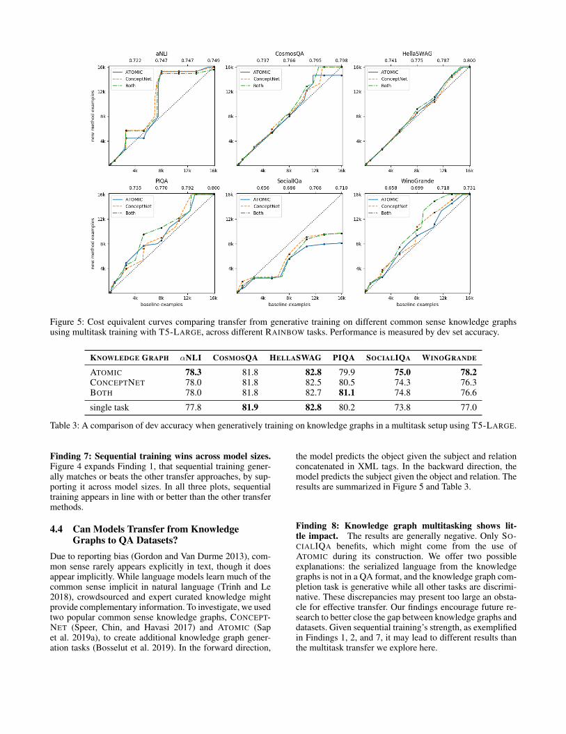
Figure 5: Cost equivalent curves comparing transfer from generative training on different common sense knowledge graphsusing multitask training with T5-LARGE, across different RAINBOW tasks. Performance is measured by dev set accuracy.

KNOWLEDGE GRAPH αNLI COSMOSQA HELLASWAG PIQA SOCIALIQA WINOGRANDE

ATOMIC 78.3 81.8 82.8 79.9 75.0 78.2CONCEPTNET 78.0 81.8 82.5 80.5 74.3 76.3BOTH 78.0 81.8 82.7 81.1 74.8 76.6

single task 77.8 81.9 82.8 80.2 73.8 77.0

Table 3: A comparison of dev accuracy when generatively training on knowledge graphs in a multitask setup using T5-LARGE.

Finding 7: Sequential training wins across model sizes.Figure 4 expands Finding 1, that sequential training gener-ally matches or beats the other transfer approaches, by sup-porting it across model sizes. In all three plots, sequentialtraining appears in line with or better than the other transfermethods.

4.4 Can Models Transfer from KnowledgeGraphs to QA Datasets?

Due to reporting bias (Gordon and Van Durme 2013), com-mon sense rarely appears explicitly in text, though it doesappear implicitly. While language models learn much of thecommon sense implicit in natural language (Trinh and Le2018), crowdsourced and expert curated knowledge mightprovide complementary information. To investigate, we usedtwo popular common sense knowledge graphs, CONCEPT-NET (Speer, Chin, and Havasi 2017) and ATOMIC (Sapet al. 2019a), to create additional knowledge graph gener-ation tasks (Bosselut et al. 2019). In the forward direction,

the model predicts the object given the subject and relationconcatenated in XML tags. In the backward direction, themodel predicts the subject given the object and relation. Theresults are summarized in Figure 5 and Table 3.

Finding 8: Knowledge graph multitasking shows lit-tle impact. The results are generally negative. Only SO-CIALIQA benefits, which might come from the use ofATOMIC during its construction. We offer two possibleexplanations: the serialized language from the knowledgegraphs is not in a QA format, and the knowledge graph com-pletion task is generative while all other tasks are discrimi-native. These discrepancies may present too large an obsta-cle for effective transfer. Our findings encourage future re-search to better close the gap between knowledge graphs anddatasets. Given sequential training’s strength, as exemplifiedin Findings 1, 2, and 7, it may lead to different results thanthe multitask transfer we explore here.

5 UNICORNFinally, we present our universal commonsense reasoningmodel, UNICORN. Motivated by Finding 1, our primary goalwith UNICORN is to provide a pretrained commonsense rea-soning model ready to be fine-tuned on other downstreamcommonsense tasks. This is analogous to how off-the-shelfT5 models are multitasked on NLP benchmarks such asGLUE and SUPERGLUE as part of their pretraining.

In order to see the limit of the best performance achiev-able, we start by multitasking T5-11B on RAINBOW. Wethen trained UNICORN on each task individually, except forWINOGRANDE which required separate handling since itevaluates models via a learning curve. For WINOGRANDE,we multitasked the other five RAINBOW datasets and thentrained on WINOGRANDE.5 In each case, we used the samehyper-parameters as UNICORN did during its initial multi-task training, extending each of the 8 combinations tried atthat stage. The best checkpoints were chosen using accuracyon dev.

SOTA on RAINBOW. We establish new SOTA on allRAINBOW datasets: αNLI (87.3%), COSMOSQA (91.8%),HELLASWAG (93.9%), PIQA (90.1%), SOCIALIQA(83.2%), and WINOGRANDE (86.6%).6

SOTA on datasets beyond RAINBOW. While SOTA re-sults on RAINBOW are encouraging, we still need to checkif UNICORN’s strong performance is confined to RAINBOWor generalizes beyond it. Thus, we evaluated on two ad-ditional commonsense benchmarks: CYCIC (94.0%) andCOMMONSENSEQA (79.3%). Again, UNICORN achievedSOTA on both.

6 Related WorkScaling Laws In contemporary machine learning, simplemethods that scale often outperform complex ones (Sutton2019). Accordingly, recent years have seen a sharp rise incompute used by state-of-the-art methods (Amodei and Her-nandez 2018). Performance gains from increasing data, pa-rameters, and training are not only reliable, but empiricallypredictable (Hestness et al. 2017; Sun et al. 2017; Rosen-feld et al. 2020; Kaplan et al. 2020). For example, Sun et al.(2017) found that models need exponential data for improve-ments in accuracy.7 These observations, that scaling is reli-able, predictable, and critical to the current successes, moti-vate our focus on evaluation based on cost-benefit trade-offs,i.e. the cost equivalent curve.

Commonsense Benchmarks Rapid progress in modelinghas led to a major challenge for NLP: the creation of suit-able benchmarks. Neural models often cue off statistical bi-ases and annotation artifacts to solve datasets without un-

5While sequential training for the RAINBOW tasks would likelyyield the best results, it would have required much more compute.

6All tasks use accuracy for evaluation except WINOGRANDEwhich uses area under the dataset size–accuracy learning curve.

7Eventually, models saturate and need super-exponential data.

derstanding tasks (Gururangan et al. 2018). To address thisissue, recent commonsense benchmarks often use adversar-ial filtering (Zellers et al. 2018; Le Bras et al. 2020): afamily of techniques that remove easily predicted examplesfrom datasets. Besides COSMOSQA, all RAINBOW tasks usethis technique. Many more common sense benchmarks ex-ist beyond what we could explore here (Roemmele, Bejan,and Gordon 2011; Levesque, Davis, and Morgenstern 2011;Mostafazadeh et al. 2016).

Transfer Learning Semi-supervised and transfer learninghave grown into cornerstones of NLP. Early work learnedunsupervised representations of words (Brown et al. 1992;Mikolov et al. 2013), while more recent work employscontextualized representations from neural language mod-els (Peters et al. 2018). Radford et al. (2018) demonstratedthat language models could be fine-tuned directly to solvea wide-variety of tasks by providing the inputs encoded astext, while Devlin et al. (2019) and others improved uponthe technique (Yang et al. 2019; Liu et al. 2019b; Lan et al.2019). Most relevant to this work, Raffel et al. (2019) in-troduced T5 which built off previous work to reframe anyNLP task as text-to-text, dispensing with the need for task-specific model adaptations.

Data Efficiency & Evaluation Other researchers havenoted the importance of cost-benefit trade-offs in evalua-tion (Schwartz et al. 2019). Dodge et al. (2019) advocate re-porting the compute-performance trade-off caused by hyper-parameter tuning for new models, and provide an estimatorfor expected validation performance as a function of hyper-parameter evaluations. In an older work, Clark and Matwin(1993) evaluated the use of qualitative knowledge in termsof saved training examples, similarly to our cost equivalentcurves. In contrast to our work, they fitted a linear trend tothe learning curve and counted examples saved rather thanplotting the numbers of examples that achieve equivalentperformance.

7 ConclusionMotivated by the fact that increased scale reliably im-proves performance for neural networks, we reevaluated ex-isting techniques based on their data efficiency. To enablesuch comparisons, we introduced a new evaluation, the costequivalent curve, which improves over traditional learningcurves by facilitating comparisons across otherwise hard-to-compare contexts. Our large-scale empirical study ana-lyzed state-of-the-art techniques for transfer on pretrainedlanguage models, focusing on learning general, common-sense knowledge and evaluating on common sense tasks.In particular, we introduced a new collection of commonsense datasets, RAINBOW, and using the lessons from ourempirical study trained a new model, UNICORN, improvingstate-of-the-art results across 8 benchmarks. We hope oth-ers find our empirical study, new evaluation, RAINBOW, andUNICORN useful in their future work.

AcknowledgementsWe would like to thank the anonymous reviewers for theirvaluable feedback. This research was supported in part byNSF (IIS-1524371), the National Science Foundation Grad-uate Research Fellowship under Grant No. DGE 1256082,DARPA CwC through ARO (W911NF15-1- 0543), DARPAMCS program through NIWC Pacific (N66001-19-2-4031),and the Allen Institute for AI. Computations on beaker.orgwere supported in part by credits from Google Cloud. TPUmachines for conducting experiments were generously pro-vided by Google through the TensorFlow Research Cloud(TFRC) program.

ReferencesAbadi, M.; Barham, P.; Chen, J.; Chen, Z.; Davis, A.; Dean, J.;Devin, M.; Ghemawat, S.; Irving, G.; Isard, M.; Kudlur, M.; Leven-berg, J.; Monga, R.; Moore, S.; Murray, D. G.; Steiner, B.; Tucker,P.; Vasudevan, V.; Warden, P.; Wicke, M.; Yu, Y.; and Zheng, X.2016. TensorFlow: A system for large-scale machine learning. In12th USENIX Symposium on Operating Systems Design and Im-plementation (OSDI 16), 265–283. URL https://www.usenix.org/system/files/conference/osdi16/osdi16-abadi.pdf.

Agirre, E.; M‘arquez, L.; and Wicentowski, R., eds. 2007. Pro-ceedings of the Fourth International Workshop on Semantic Eval-uations (SemEval-2007). Prague, Czech Republic: Association forComputational Linguistics.

Amodei, D.; and Hernandez, D. 2018. AI and Compute. URLhttps://openai.com/blog/ai-and-compute/.

Bar Haim, R.; Dagan, I.; Dolan, B.; Ferro, L.; Giampiccolo, D.;Magnini, B.; and Szpektor, I. 2006. The second PASCAL recog-nising textual entailment challenge .

Barlow, R.; Bartholomew, D.; Bremner, J.; and Brunk, H.1972. Statistical Inference Under Order Restrictions: The The-ory and Application of Isotonic Regression. J. Wiley. ISBN9780471049708.

Bentivogli, L.; Dagan, I.; Dang, H. T.; Giampiccolo, D.; andMagnini, B. 2009. The Fifth PASCAL Recognizing Textual En-tailment Challenge .

Bhagavatula, C.; Le Bras, R.; Malaviya, C.; Sakaguchi, K.; Holtz-man, A.; Rashkin, H.; Downey, D.; Yih, S. W.-t.; and Choi, Y. 2020.Abductive commonsense reasoning. ICLR .

Bisk, Y.; Zellers, R.; Le Bras, R.; Gao, J.; and Choi, Y. 2020. PIQA:Reasoning about Physical Commonsense in Natural Language. InThirty-Fourth AAAI Conference on Artificial Intelligence.

Bosselut, A.; Rashkin, H.; Sap, M.; Malaviya, C.; Celikyilmaz, A.;and Choi, Y. 2019. COMET: Commonsense Transformers for Au-tomatic Knowledge Graph Construction. In Proceedings of the57th Annual Meeting of the Association for Computational Lin-guistics (ACL).

Brown, P. F.; Della Pietra, V. J.; deSouza, P. V.; Lai, J. C.; andMercer, R. L. 1992. Class-Based n-gram Models of Natural Lan-guage. Computational Linguistics 18(4): 467–480. URL https://www.aclweb.org/anthology/J92-4003.

Caruana, R. 1995. Learning Many Related Tasks at theSame Time with Backpropagation. In Tesauro, G.; Touret-zky, D. S.; and Leen, T. K., eds., Advances in Neural Infor-mation Processing Systems 7, 657–664. MIT Press. URLhttp://papers.nips.cc/paper/959-learning-many-related-tasks-at-the-same-time-with-backpropagation.pdf.

Clark, C.; Lee, K.; Chang, M.-W.; Kwiatkowski, T.; Collins, M.;and Toutanova, K. 2019. BoolQ: Exploring the Surprising Diffi-culty of Natural Yes/No Questions. In Proceedings of NAACL-HLT2019.

Clark, P.; and Matwin, S. 1993. Using qualitative models to guideinductive learning. In Proceedings of the 1993 international con-ference on machine learning.

Dagan, I.; Glickman, O.; and Magnini, B. 2006. The PASCALrecognising textual entailment challenge. In Machine learningchallenges. evaluating predictive uncertainty, visual object classi-fication, and recognising tectual entailment, 177–190. Springer.

De Marneffe, M.-C.; Simons, M.; and Tonhauser, J. 2019. TheCommitmentBank: Investigating projection in naturally occurringdiscourse. To appear in proceedings of Sinn und Bedeutung 23.Data can be found at https://github.com/mcdm/CommitmentBank/.

Devlin, J.; Chang, M.-W.; Lee, K.; and Toutanova, K. 2019. BERT:Pre-training of Deep Bidirectional Transformers for LanguageUnderstanding. In Proceedings of the 2019 Conference of theNorth American Chapter of the Association for ComputationalLinguistics: Human Language Technologies, Volume 1 (Long andShort Papers), 4171–4186. Minneapolis, Minnesota: Associationfor Computational Linguistics. doi:10.18653/v1/N19-1423. URLhttps://www.aclweb.org/anthology/N19-1423.

Dodge, J.; Gururangan, S.; Card, D.; Schwartz, R.; and Smith,N. A. 2019. Show Your Work: Improved Reporting of Experi-mental Results. In Proceedings of the 2019 Conference on Em-pirical Methods in Natural Language Processing and the 9th In-ternational Joint Conference on Natural Language Processing(EMNLP-IJCNLP), 2185–2194. Hong Kong, China: Associationfor Computational Linguistics. doi:10.18653/v1/D19-1224. URLhttps://www.aclweb.org/anthology/D19-1224.

Dolan, W. B.; and Brockett, C. 2005. Automatically constructinga corpus of sentential paraphrases. In Proceedings of the Interna-tional Workshop on Paraphrasing.

Giampiccolo, D.; Magnini, B.; Dagan, I.; and Dolan, B. 2007. Thethird PASCAL recognizing textual entailment challenge. In Pro-ceedings of the ACL-PASCAL workshop on textual entailment andparaphrasing, 1–9. Association for Computational Linguistics.

Gordon, J.; and Van Durme, B. 2013. Reporting bias and knowl-edge acquisition. In Proceedings of the 2013 workshop on Auto-mated knowledge base construction, 25–30. ACM.

Gururangan, S.; Swayamdipta, S.; Levy, O.; Schwartz, R.; Bow-man, S.; and Smith, N. A. 2018. Annotation Artifacts in NaturalLanguage Inference Data. In NAACL. URL https://www.aclweb.org/anthology/N18-2017/.

Hestness, J.; Narang, S.; Ardalani, N.; Diamos, G. F.; Jun, H.;Kianinejad, H.; Patwary, M. M. A.; Yang, Y.; and Zhou, Y.2017. Deep Learning Scaling is Predictable, Empirically. ArXivabs/1712.00409.

Huang, L.; Le Bras, R.; Bhagavatula, C.; and Choi, Y. 2019. Cos-mos QA: Machine Reading Comprehension with Contextual Com-monsense Reasoning. In EMNLP/IJCNLP.

Kaplan, J.; McCandlish, S.; Henighan, T.; Brown, T. B.; Chess,B.; Child, R.; Gray, S.; Radford, A.; Wu, J.; and Amodei, D.2020. Scaling laws for neural language models. arXiv preprintarXiv:2001.08361 .

Khashabi, D.; Chaturvedi, S.; Roth, M.; Upadhyay, S.; and Roth,D. 2018. Looking beyond the surface: A challenge set for read-ing comprehension over multiple sentences. In Proceedings of the

2018 Conference of the North American Chapter of the Associa-tion for Computational Linguistics: Human Language Technolo-gies, Volume 1 (Long Papers), 252–262.

Khashabi, D.; Min, S.; Khot, T.; Sabhwaral, A.; Tafjord, O.; Clark,P.; and Hajishirzi, H. 2020. UnifiedQA: Crossing Format Bound-aries With a Single QA System. arXiv preprint .

Lan, Z.; Chen, M.; Goodman, S.; Gimpel, K.; Sharma, P.; and Sori-cut, R. 2019. Albert: A lite bert for self-supervised learning oflanguage representations. arXiv preprint arXiv:1909.11942 .

Le Bras, R.; Swayamdipta, S.; Bhagavatula, C.; Zellers, R.; Peters,M. E.; Sabharwal, A.; and Choi, Y. 2020. Adversarial Filters ofDataset Biases. ArXiv abs/2002.04108.

Levesque, H. J.; Davis, E.; and Morgenstern, L. 2011. The Wino-grad schema challenge. In AAAI Spring Symposium: Logical For-malizations of Commonsense Reasoning, volume 46, 47.

Liu, X.; He, P.; Chen, W.; and Gao, J. 2019a. Multi-Task DeepNeural Networks for Natural Language Understanding. In Pro-ceedings of the 57th Annual Meeting of the Association for Com-putational Linguistics, 4487–4496. Florence, Italy: Associationfor Computational Linguistics. doi:10.18653/v1/P19-1441. URLhttps://www.aclweb.org/anthology/P19-1441.

Liu, Y.; Ott, M.; Goyal, N.; Du, J.; Joshi, M.; Chen, D.; Levy, O.;Lewis, M.; Zettlemoyer, L.; and Stoyanov, V. 2019b. Roberta:A robustly optimized bert pretraining approach. arXiv preprintarXiv:1907.11692 .

Ma, K.; Francis, J.; Lu, Q.; Nyberg, E.; and Oltramari, A. 2019.Towards Generalizable Neuro-Symbolic Systems for Common-sense Question Answering. In Proceedings of the First Workshopon Commonsense Inference in Natural Language Processing, 22–32. Hong Kong, China: Association for Computational Linguis-tics. doi:10.18653/v1/D19-6003. URL https://www.aclweb.org/anthology/D19-6003.

McCarthy, J. 1959. Programs with Common Sense. In Proceedingsof the Teddington Conference on the Mechanization of ThoughtProcesses, 75–91. London: Her Majesty’s Stationary Office.

Mikolov, T.; Sutskever, I.; Chen, K.; Corrado, G. S.; andDean, J. 2013. Distributed Representations of Words andPhrases and their Compositionality. In Burges, C. J. C.;Bottou, L.; Welling, M.; Ghahramani, Z.; and Weinberger,K. Q., eds., Advances in Neural Information ProcessingSystems 26, 3111–3119. Curran Associates, Inc. URLhttp://papers.nips.cc/paper/5021-distributed-representations-of-words-and-phrases-and-their-compositionality.pdf.

Mostafazadeh, N.; Chambers, N.; He, X.; Parikh, D.; Batra, D.;Vanderwende, L.; Kohli, P.; and Allen, J. 2016. A Corpus andCloze Evaluation for Deeper Understanding of Commonsense Sto-ries. In Proceedings of the 2016 Conference of the North AmericanChapter of the Association for Computational Linguistics: HumanLanguage Technologies, 839–849. San Diego, California: Associ-ation for Computational Linguistics. doi:10.18653/v1/N16-1098.URL https://www.aclweb.org/anthology/N16-1098.

Pedregosa, F.; Varoquaux, G.; Gramfort, A.; Michel, V.; Thirion,B.; Grisel, O.; Blondel, M.; Prettenhofer, P.; Weiss, R.; Dubourg,V.; et al. 2011. Scikit-learn: Machine learning in Python. the Jour-nal of machine Learning research 12: 2825–2830.

Peters, M.; Neumann, M.; Iyyer, M.; Gardner, M.; Clark, C.; Lee,K.; and Zettlemoyer, L. 2018. Deep Contextualized Word Repre-sentations. In Proceedings of the 2018 Conference of the NorthAmerican Chapter of the Association for Computational Linguis-tics: Human Language Technologies, Volume 1 (Long Papers),

2227–2237. New Orleans, Louisiana: Association for Computa-tional Linguistics. doi:10.18653/v1/N18-1202. URL https://www.aclweb.org/anthology/N18-1202.

Pilehvar, M. T.; and Camacho-Collados, J. 2019. WiC: The Word-in-Context Dataset for Evaluating Context-Sensitive Meaning Rep-resentations. In Proceedings of NAACL-HLT.

Poliak, A.; Haldar, A.; Rudinger, R.; Hu, J. E.; Pavlick, E.; White,A. S.; and Van Durme, B. 2018. Collecting Diverse Natural Lan-guage Inference Problems for Sentence Representation Evaluation.In Proceedings of EMNLP.

Pratt, L.; Mostow, J.; and Kamm, C. 1991. Direct Transfer ofLearned Information Among Neural Networks. In AAAI.

Pruksachatkun, Y.; Phang, J.; Liu, H.; Htut, P. M.; Zhang, X.; Pang,R. Y.; Vania, C.; Kann, K.; and Bowman, S. R. 2020. Intermediate-Task Transfer Learning with Pretrained Models for Natural Lan-guage Understanding: When and Why Does It Work? arXivpreprint arXiv:2005.00628 .

Radford, A.; Narasimhan, K.; Salimans, T.; and Sutskever,I. 2018. Improving language understanding by genera-tive pre-training. URL https://s3-us-west-2.amazonaws.com/openai-assets/research-covers/language-unsupervised/language understanding paper.pdf.

Raffel, C.; Shazeer, N.; Roberts, A.; Lee, K.; Narang, S.; Matena,M.; Zhou, Y.; Li, W.; and Liu, P. J. 2019. Exploring the Limits ofTransfer Learning with a Unified Text-to-Text Transformer. arXive-prints .

Rajpurkar, P.; Zhang, J.; Lopyrev, K.; and Liang, P. 2016. SQuAD:100,000+ Questions for Machine Comprehension of Text. In Pro-ceedings of EMNLP, 2383–2392. Association for ComputationalLinguistics.

Roemmele, M.; Bejan, C. A.; and Gordon, A. S. 2011. Choice ofplausible alternatives: An evaluation of commonsense causal rea-soning. In 2011 AAAI Spring Symposium Series.

Rosenfeld, J. S.; Rosenfeld, A.; Belinkov, Y.; and Shavit, N.2020. A Constructive Prediction of the Generalization Error AcrossScales. In International Conference on Learning Representations.URL https://openreview.net/forum?id=ryenvpEKDr.

Rudinger, R.; Naradowsky, J.; Leonard, B.; and Van Durme, B.2018. Gender Bias in Coreference Resolution. In Proceedingsof NAACL-HLT.

Sakaguchi, K.; Le Bras, R.; Bhagavatula, C.; and Choi, Y. 2020.WINOGRANDE: An Adversarial Winograd Schema Challenge atScale. In AAAI.

Sap, M.; Le Bras, R.; Allaway, E.; Bhagavatula, C.; Lourie, N.;Rashkin, H.; Roof, B.; Smith, N. A.; and Choi, Y. 2019a. Atomic:An atlas of machine commonsense for if-then reasoning. In Pro-ceedings of the AAAI Conference on Artificial Intelligence, vol-ume 33, 3027–3035.

Sap, M.; Rashkin, H.; Chen, D.; Le Bras, R.; and Choi, Y. 2019b.Social IQA: Commonsense Reasoning about Social Interactions.In EMNLP 2019.

Schwartz, R.; Dodge, J.; Smith, N. A.; and Etzioni, O. 2019. Greenai. arXiv preprint arXiv:1907.10597 .

Socher, R.; Perelygin, A.; Wu, J.; Chuang, J.; Manning, C. D.; Ng,A.; and Potts, C. 2013. Recursive deep models for semantic com-positionality over a sentiment treebank. In Proceedings of EMNLP,1631–1642.

Speer, R.; Chin, J.; and Havasi, C. 2017. ConceptNet 5.5: An OpenMultilingual Graph of General Knowledge. In Proceedings of theThirty-First AAAI Conference on Artificial Intelligence, AAAI’17,4444–4451. AAAI Press.

Sun, C.; Shrivastava, A.; Singh, S.; and Gupta, A. 2017. Revisitingunreasonable effectiveness of data in deep learning era. In Pro-ceedings of the IEEE international conference on computer vision,843–852.

Sutton, R. S. 2019. The Bitter Lesson. URL http://incompleteideas.net/IncIdeas/BitterLesson.html.

Talmor, A.; Herzig, J.; Lourie, N.; and Berant, J. 2019. Com-monsenseQA: A Question Answering Challenge Targeting Com-monsense Knowledge. In Proceedings of the 2019 Conference ofthe North American Chapter of the Association for ComputationalLinguistics: Human Language Technologies, Volume 1 (Long andShort Papers), 4149–4158. Minneapolis, Minnesota: Associationfor Computational Linguistics. doi:10.18653/v1/N19-1421. URLhttps://www.aclweb.org/anthology/N19-1421.

Tange, O. 2011. GNU Parallel - The Command-Line Power Tool.;login: The USENIX Magazine 36(1): 42–47. doi:10.5281/zenodo.16303. URL http://www.gnu.org/s/parallel.

Trinh, T. H.; and Le, Q. V. 2018. A simple method for common-sense reasoning. arXiv preprint arXiv:1806.02847 .

Vaswani, A.; Shazeer, N.; Parmar, N.; Uszkoreit, J.; Jones, L.;Gomez, A. N.; Kaiser, Ł.; and Polosukhin, I. 2017. Attention isall you need. In Advances in neural information processing sys-tems, 5998–6008.

Vu, T.; Wang, T.; Munkhdalai, T.; Sordoni, A.; Trischler, A.;Mattarella-Micke, A.; Maji, S.; and Iyyer, M. 2020. Exploringand predicting transferability across nlp tasks. arXiv preprintarXiv:2005.00770 .

Wang, A.; Pruksachatkun, Y.; Nangia, N.; Singh, A.; Michael, J.;Hill, F.; Levy, O.; and Bowman, S. R. 2019a. SuperGLUE: A Stick-ier Benchmark for General-Purpose Language Understanding Sys-tems. arXiv preprint 1905.00537 .

Wang, A.; Singh, A.; Michael, J.; Hill, F.; Levy, O.; and Bowman,S. R. 2019b. GLUE: A Multi-Task Benchmark and Analysis Plat-form for Natural Language Understanding. In the Proceedings ofICLR.

Warstadt, A.; Singh, A.; and Bowman, S. R. 2018. Neural NetworkAcceptability Judgments. arXiv preprint 1805.12471 .

Williams, A.; Nangia, N.; and Bowman, S. R. 2018. A Broad-Coverage Challenge Corpus for Sentence Understanding throughInference. In Proceedings of NAACL-HLT.

Williams, R. J.; and Zipser, D. 1989. A Learning Algorithm forContinually Running Fully Recurrent Neural Networks. NeuralComputation 1(2): 270–280.

Winograd, T. 1972. Understanding natural language. Cognitivepsychology 3(1): 1–191.

Yang, Z.; Dai, Z.; Yang, Y.; Carbonell, J.; Salakhutdinov, R. R.;and Le, Q. V. 2019. Xlnet: Generalized autoregressive pretrainingfor language understanding. In Advances in neural informationprocessing systems, 5753–5763.

Zellers, R.; Bisk, Y.; Schwartz, R.; and Choi, Y. 2018. SWAG:A Large-Scale Adversarial Dataset for Grounded CommonsenseInference. In Proceedings of the 2018 Conference on EmpiricalMethods in Natural Language Processing (EMNLP).

Zellers, R.; Holtzman, A.; Bisk, Y.; Farhadi, A.; and Choi, Y. 2019.HellaSwag: Can a Machine Really Finish Your Sentence? In ACL.

Zhang, S.; Liu, X.; Liu, J.; Gao, J.; Duh, K.; and Durme, B. V. 2018.ReCoRD: Bridging the Gap between Human and Machine Com-monsense Reading Comprehension. arXiv preprint 1810.12885 .

Zhang, S.; Rudinger, R.; Duh, K.; and Van Durme, B. 2017. Ordi-nal Common-sense Inference. Transactions of the Association forComputational Linguistics 5: 379–395. doi:10.1162/tacl a 00068.URL https://www.aclweb.org/anthology/Q17-1027.

Zhu, Y.; Pang, L.; Lan, Y.; and Cheng, X. 2020. L2R²: Leverag-ing Ranking for Abductive Reasoning. In Proceedings of the 43rdInternational ACM SIGIR Conference on Research and Develop-ment in Information Retrieval, SIGIR ’20. doi:10.1145/3397271.3401332. URL https://doi.org/10.1145/3397271.3401332.

A Cost Equivalent CurvesSection 2 discusses the intuitions, assumptions, and visual-ization of cost equivalent curves at a high level. This ap-pendix provides additional discussion as well as technicaldetails for implementing cost equivalent curves.

The aim of cost equivalent curves is to visualize how aninnovation impacts a cost-benefit trade-off, in a compact andintuitive way. Since cost equivalent curves are more generalthan the use case explored in this work (dataset size / perfor-mance trade-offs), we’ll introduce more general terminol-ogy for discussing them, borrowing from the experimentaldesign literature. The control is the baseline approach (e.g.,single task training), while the treatment is the new approachor innovation (e.g., multitask or sequential training). Benefitis a quantitative measure of how good the outcome is, likeaccuracy, while cost measures what we pay to get it, suchas dataset size or even dollars. Thus, cost equivalent curvescan visualize how sequential training (the treatment) reducesdata usage (the cost) compared to single task training (thecontrol) when trying to achieve high accuracy (the benefit).Similarly, cost equivalent curves could visualize how Gaus-sian process optimization reduces hyper-parameter evalua-tions compared to random search when trying to achieve lowperplexity on a language modeling task.

To construct cost equivalent curves, the main assump-tion is that the cost and benefit have a continuous, strictlymonotonic (most often increasing) relationship. For machinelearning, this assumption is satisfied empirically when usingmeasures like expected cross-entropy against parameters,data, and compute (Kaplan et al. 2020). Since the cost andbenefit share a monotonic relationship, we estimate the cost-benefit trade-offs using isotonic regression (Barlow et al.1972). Concretely, we test the control and the treatment ata bunch of different costs, and measure the benefit. Then,we fit a curve to the control’s results, fc, and a curve to thetreatment’s results, ft. Since the cost equivalent curve, g,maps the control costs to the treatment costs achieving thesame benefit, we can estimate it as:

g = f−1t ◦ fcThat is, we compose the inverse cost-benefit curve for thetreatment with the cost-benefit curve for the control. Theinverse is guaranteed to exist because we assumed that thecost-benefit trade-offs are strictly monotonic.

Our implementation uses isotonic regression as imple-mented in scikit-learn (Pedregosa et al. 2011). To estimatethe inverse curve, we switch the inputs and the outputs inthe regression. The code may be found at https://github.com/allenai/rainbow.

B DatasetsOur empirical study investigates transferring common sensefrom multisets (dataset collections) to various end tasks.Section 3 presented a new multiset, RAINBOW, for com-mon sense transfer. In this appendix, Appendix B.1 de-scribes each end task we evaluated, Appendix B.2 expandson RAINBOW and the other multisets we tried, and Ap-pendix B.3 details the knowledge graphs we used.

B.1 TasksSix tasks, αNLI, COSMOSQA, HELLASWAG, PIQA, SO-CIALIQA, and WINOGRANDE, compose RAINBOW, as dis-cussed in Section 3. Our experiments also use all six ofthese datasets as end tasks. In addition, we evaluated onCOMMONSENSEQA, JOCI, and CYCIC. Each dataset is de-scribed below:

αNLI (Bhagavatula et al. 2020) challenges models to in-fer the best explanation8 connecting the beginning and end-ing of a story. Concretely, αNLI presents models with thefirst and last sentences of a three sentence story. The modelmust choose among two alternative middles based on whichprovides the most plausible explanation.

COSMOSQA (Huang et al. 2019) tests models’ readingcomprehension by asking them to read in-between the lines.Each example presents a short passage along with a questiondealing with commonsense causes, effects, inferences andcounterfactuals drawn from the passage. To solve the task,models must choose the best answer among four candidates.

HELLASWAG (Zellers et al. 2019) takes a context sen-tence and generates multiple completions using a languagemodel. The machine generated endings often break com-monsense world understanding, making it easy for hu-mans to distinguish them from the original ending. In addi-tion, HELLASWAG uses adversarial filtering (Zellers et al.2018) to select the three distractor endings only from amongthose difficult for models to detect.

PIQA (Bisk et al. 2020) probes models’ physical com-monsense knowledge through goal-oriented question an-swering problems. The questions often explore object affor-dances, presenting a goal (e.g., “How do I find somethinglost on a carpet?”) and then offering two solutions (such as“Put a solid seal on the end of your vacuum and turn it on”vs. “Put a hair net on the end of your vacuum and turn iton”). Models choose the best solution to solve the problem.

SOCIALIQA (Sap et al. 2019b) leverages ATOMIC (Sapet al. 2019a) to crowdsource a three-way multiple-choicebenchmark evaluating the social and emotional commonsense possessed by models. Questions explore people’s mo-tivations and reactions in a variety of social situations.

WINOGRANDE (Sakaguchi et al. 2020) takes inspirationfrom winograd schemas (Winograd 1972; Levesque, Davis,and Morgenstern 2011) to create a large-scale dataset ofcoreference resolution problems requiring both physical andsocial common sense. Each question presents a sentencewith a blank where a pronoun might be and two options tofill it. The questions often come in pairs where a single wordchanges between them, flipping which option is correct.

8Also known as abductive reasoning.

COMMONSENSEQA (Talmor et al. 2019) offers general,challenging, common sense questions in a multiple-choiceformat. By construction, each question requires fine-grainedworld knowledge to distinguish between highly similarconcepts. In particular, COMMONSENSEQA crowdsourcesquestions by presenting annotators with three related con-cepts drawn from CONCEPTNET (Speer, Chin, and Havasi2017). The annotators then create three questions, each pick-ing out one of the concepts as the correct answer. To increasethe dataset’s difficulty, an additional distractor from CON-CEPTNET as well as one authored by a human were addedto each question, for a total of five options.

CYCIC9 offers five-way multiple-choice questions thattouch on both common sense reasoning and knowledge overtopics such as arithmetic, logic, time, and locations.

JOCI (Zhang et al. 2017) (JHU Ordinal CommonsenseInference) generalizes natural language inference (NLI) tolikely implications. Each problem presents a context fol-lowed by a hypothesis. In contrast to traditional NLI whichexplores hard, logical implications, JOCI instead exploreslikely inferences from the context. Thus, each examplecomes with an ordinal label of the likelihood: very likely,likely, plausible, technically possible, or impossible. In con-trast to Zhang et al. (2017), we treat the task as five-wayclassification and evaluate it with accuracy in order to makeit uniform with other end tasks we explore.

B.2 MultisetsIn addition to RAINBOW, we use two other multisets fortransfer. All three are described below.

GLUE (Wang et al. 2019b) measures natural languageunderstanding by evaluating models on a suite of classi-fication tasks. In particular, GLUE contains tasks for lin-guistic acceptability (Warstadt, Singh, and Bowman 2018),sentiment analysis (Socher et al. 2013), paraphrase (Dolanand Brockett 2005; Agirre, M‘arquez, and Wicentowski2007)10, natural language inference (sometimes constructedfrom other datasets) (Williams, Nangia, and Bowman 2018;Rajpurkar et al. 2016; Dagan, Glickman, and Magnini 2006;Bar Haim et al. 2006; Giampiccolo et al. 2007; Bentivogliet al. 2009; Levesque, Davis, and Morgenstern 2011), andgeneral diagnostics.

SUPERGLUE (Wang et al. 2019a) provides a more chal-lenging successor to GLUE, measuring natural languageunderstanding with a broader range of more complex tasks.Specifically, SUPERGLUE comprises tasks for identifyingwhen speakers implicitly assert something (De Marneffe,Simons, and Tonhauser 2019), determining cause-effect re-lationships (Roemmele, Bejan, and Gordon 2011), reading

9The CYCIC dataset and leaderboard may be found at https://leaderboard.allenai.org/cycic

10For more on Quora Question Pairs see https://www.quora.com/q/quoradata/First-Quora-Dataset-Release-Question-Pairs.

comprehension (Khashabi et al. 2018; Zhang et al. 2018),natural language inference (Dagan, Glickman, and Magnini2006; Bar Haim et al. 2006; Giampiccolo et al. 2007; Ben-tivogli et al. 2009; Poliak et al. 2018), word sense disam-biguation (Pilehvar and Camacho-Collados 2019), winogradschemas (Levesque, Davis, and Morgenstern 2011), true-false question answering (Clark et al. 2019), and gender biasdiagnostics (Rudinger et al. 2018).

RAINBOW combines the six common sense benchmarksas we proposed in Section 3: αNLI (Bhagavatula et al.2020), COSMOSQA (Huang et al. 2019), HELLASWAG(Zellers et al. 2019), PIQA (Bisk et al. 2020), SOCIALIQA(Sap et al. 2019b), and WINOGRANDE (Sakaguchi et al.2020). These multiple-choice datasets each measure dif-ferent aspects of common sense, from likely sequences ofevents, to instrumental knowledge in physical situations, totheory of mind and social common sense.

B.3 Knowledge GraphsIn addition to multisets, we explored common sense transferfrom the following knowledge graphs in Section 4.4:

CONCEPTNET (Speer, Chin, and Havasi 2017) combinesboth expert curated and crowdsourced knowledge from vari-ous sources into a graph of concepts and relations. A conceptis a short natural language word or phrase, such as “water”.Connecting concepts, there’s a commonly used set of canon-ical relations like ATLOCATION. For example, CONCEPT-NET contains the triple: “water” ATLOCATION “river”.CONCEPTNET contains a significant amount of informationbeyond common sense; however, the common sense subsettends to focus on knowledge about objects and things.

ATOMIC (Sap et al. 2019a) offers a rich source of knowl-edge about the relationships between events and commonsense inferences about them. ATOMIC connects events de-scribed in natural language using relations that expressthings like pre-conditions, post-conditions, and plausible in-ferences based on the event. For example, ATOMIC con-tains the triple: “PersonX makes PersonY’s coffee” OREACT“PersonY will be grateful”, where OREACT denotes the pa-tient’s (PersonY’s) reaction.

C Training and EvaluationThis appendix describes the technical details of our trainingand evaluation setup, to help reproduce our experiments.

C.1 Model and ImplementationAll of our experiments are run with the state-of-the-art T5model (Raffel et al. 2019). T5 is a text-to-text model builton top of the transformer architecture (Vaswani et al. 2017).It has an encoder-decoder structure and is pretrained us-ing a combination of masked language modeling (Devlinet al. 2019) and multitask training on a large collection ofNLP datasets. As a text-to-text model, T5 frames every NLP

problem as mapping input text to output text. All struc-tural information in the input is linearized into a sequenceof text, similarly to Radford et al. (2018), and all output isgenerated as a string when making predictions. For train-ing, T5 uses teacher forcing (Williams and Zipser 1989),i.e. maximum likelihood; for testing, T5 greedily decodesthe generated text. Thus, for T5 to solve a task, one mustfirst apply some straightforward preprocessing to frame it astext-to-text. Appendix C.2 describes the preprocessing weperformed in more detail. Lastly, T5 is available in severalmodel sizes: small (60M parameters), base (220M param-eters), large (770M parameters), 3B (3B parameters), and11B (11B parameters). For more information on T5 and itspretraining, see Raffel et al. (2019).

Our experiments use the original implementation,code, and weights for T5, which are publicly availableat https://github.com/google-research/text-to-text-transfer-transformer. Our code uses the original T5 implementationunmodified, only extending it with our own dataset prepro-cessing, reading, and task mixing. For deep learning op-erations, the implementation uses tensorflow (Abadi et al.2016). Our code is available at https://github.com/allenai/rainbow.

C.2 PreprocessingTo model tasks as text-to-text, we need to convert theirinputs and outputs into strings. Our preprocessing firstprepends a string to each example signifying its dataset, e.g.[socialiqa]: for the SOCIALIQA task. Next, it wrapseach feature in XML-like brackets with a unique tag iden-tifying the feature, then joins them all together with new-line characters. Figure 6 depicts an example from WINO-GRANDE. Preprocessing for other tasks is similar.

Figure 6: An example of the dataset preprocessing appliedto an instance from WINOGRANDE.

C.3 Training and Hyper-parameter TuningFollowing Raffel et al. (2019), we converted all tasks to text-to-text and used teacher forcing (Williams and Zipser 1989)as the training objective, with greedy decoding for predic-tions. Our implementation reused the training and evalua-tion code from the original T5 paper. For leaderboard sub-missions and test set evaluations, we built UNICORN off ofT5-11B. For all other experiments, we used T5-LARGE ex-cept when experiments specifically explore the impact ofsize, in which case the model size was explicitly indicated.

Hyper-parameters which were not set manually weretuned via grid search. In general, the fixed hyper-parameters

and the grid used for search depended on the group of ex-periments, as outlined below. All hyper-parameters not men-tioned were identical to those used in Raffel et al. (2019).

Leaderboard Submissions For leaderboard submissionsand test set evaluations, T5-11B was initially multitaskedon RAINBOW with an equal task mixing rate for 25,000 gra-dient updates using different hyper-parameter combinationsto produce the UNICORNs. We then trained each on the endtasks separately for 25,000 gradient updates, saving a check-point every 2,500. The 10 most recent checkpoints were keptfor early stopping, using dev set accuracy to choose the bestcheckpoint for evaluation. The grid search explored learningrates of 4e-3, 2e-3, 1e-3, and 5e-4 as well as batch sizes of16 and 32.

Investigatory Experiments Experiments which were notevaluated on the test set or submitted to a leaderboard usedthe T5-LARGE model as a starting point, unless explicitlynoted otherwise (e.g., in experiments exploring the impactof model size). Training was carried out for 50,000 gradi-ent updates, saving a checkpoint every 5,000 and keepingthe 10 most recent. The batch size was fixed to 16. Gridsearch explored learning rates of 4e-3, 1e-3, and 2.5e-4. De-pending on the specific experiment, other hyper-parameterswere explored as well. For models trained on full datasets(rather than learning curves), we explored equal and datasetsize-weighted mixing rates when multitasking. In sequentialtraining, this meant that these rates were tried during the ini-tial multitask training before training on the end task alone.For transferring knowledge graphs, we also explored pre-dicting the subject-relation-object tuples in forward, back-ward, and bidirectional configurations. When producinglearning curves, i.e. training the model on subsets of the fulldata, we used the equal mixing rate for all mixtures and theforward direction for knowledge graph transfer. Given theextensiveness of these experiments, we chose not to evalu-ate these models on the test sets to avoid test leakage; thus,reported results for these experiments are always the bestscore on dev.

For transfer techniques requiring two stages of training(i.e. multitask fine-tune and sequential training), we reusedthe hyper-parameters from the first stage of training in thesecond stage. For all tasks, we used accuracy as the evalua-tion metric.

To facilitate reproducibility and future research, we re-lease results for all of our experiments, including hyper-parameter tuning. Download the results at https://github.com/allenai/rainbow. These tables contain all model eval-uations and all hyper-parameter combinations tried in anygiven experiment.

C.4 Hardware, Software, and ComputeAll experiments were run on Google Cloud using twoGoogle Compute Engine virtual machine (VM) instancescommunicating with various TPUs. Experimental resultswere saved into Google Cloud Storage. Each VM had 20vCPUs with 75GB of memory and ran Debian 9 (Stretch).

One VM used Intel Skylake vCPUs while the other used In-tel Haswell. Specific versions of libraries and other depen-dencies used are available and tracked in the code repository.

For hardware acceleration, we ran all the experiments us-ing v3-8 TPUs when building off of T5-LARGE or smaller.For T5-SMALL and T5-LARGE we used a model paral-lelism of 8, while for T5-BASE we used 4. The T5-11Bmodels were trained using TPU v2-256 and v3-256s with amodel parallelism of 16. Training times usually took severalhours per run, so we ran many experiments in parallel on theVMs using GNU Parallel (Tange 2011).

D LeaderboardsAs discussed in Section 5, UNICORN achieves state-of-the-art performance across a number of popular commonsensebenchmarks. This appendix collects those results along withthe leaderboards’ previous state-of-the-art and other usefulbaseline submissions for comparison.

αNLI

MODEL ACCURACY

BERT-LARGE (Devlin et al. 2019) 66.8%ROBERTA-LARGE (Liu et al. 2019b) 83.9%L2R2 (Zhu et al. 2020) 86.8%UNICORN 87.3%HUMAN 92.9%

Table 4: αNLI leaderboard submissions.

COSMOSQA

MODEL ACCURACY

ROBERTA-LARGE (Liu et al. 2019b) 83.5%ALBERT-XXLARGE (Lan et al. 2019) 85.4%T5-11B (Raffel et al. 2019) 90.3%UNICORN 91.8%HUMAN 94.0%

Table 5: COSMOSQA leaderboard submissions.

HELLASWAG

MODEL ACCURACY

ROBERTA-LARGE (Liu et al. 2019b) 81.7%HYKAS+CSKG (Ma et al. 2019) 85.0%ROBERTA-LARGE ENSEMBLE(Liu et al. 2019b)

85.5%

UNICORN 93.9%HUMAN 95.6%

Table 6: HELLASWAG leaderboard submissions.

Since COMMONSENSEQA used CONCEPTNET in itsconstruction, its authors have split leaderboard submissions

PIQA

MODEL ACCURACY

BERT-LARGE (Devlin et al. 2019) 66.7%ROBERTA-LARGE (Liu et al. 2019b) 79.4%UNIFIEDQA-3B (Khashabi et al. 2020) 85.3%UNICORN 90.1%HUMAN 94.9%

Table 7: PIQA leaderboard submissions.

SOCIALIQA

MODEL ACCURACY

ROBERTA-LARGE (Liu et al. 2019b) 76.7%UNIFIEDQA-3B (Khashabi et al. 2020) 79.8%UGAMIX 80.0%UNICORN 83.2%HUMAN 88.1%

Table 8: SOCIALIQA leaderboard submissions.

WINOGRANDE

MODEL AUC

BERT-LARGE (Devlin et al. 2019) 52.9%ROBERTA-LARGE (Liu et al. 2019b) 66.4%UNIFIEDQA-11B (Khashabi et al. 2020) 85.7%UNICORN 86.6%HUMAN 94.0%

Table 9: WINOGRANDE leaderboard submissions. AUC isthe area under the dataset-size vs. accuracy learning curve.

CYCIC

MODEL ACCURACY

ROBERTA-LARGE (Liu et al. 2019b) 91.3%PRV2 91.4%UNICORN 94.0%HUMAN 90.0%

Table 10: CYCIC leaderboard submissions.

COMMONSENSEQA

MODEL ACCURACY

ROBERTA-LARGE (Liu et al. 2019b) 72.1%T5-11B (Raffel et al. 2019) 78.1%UNIFIEDQA-11B (Khashabi et al. 2020) 79.1%UNICORN 79.3%HUMAN 88.9%

Table 11: COMMONSENSEQA leaderboard submissions.

into two categories: models that do and that do not use CON-CEPTNET. Models using CONCEPTNET can gain an advan-tage by eliminating the human authored distractor options.UNICORN holds the current state-of-the-art among modelswhich do not use CONCEPTNET. The state-of-the-art modelusing CONCEPTNET combines the knowledge graph withALBERT (Lan et al. 2019)11 and scores 79.5% accuracy.

Hyper-parameters For each of the submissions, we usedthe following hyper-parameters. αNLI used a learning rateof 5e-4 and a batch size of 16. COSMOSQA used a learn-ing rate of 2e-3 and a batch size of 32. HELLASWAG useda learning rate of 2e-3 and a batch size of 32. PIQA useda learning rate of 2e-3 and a batch size of 32. SOCIALIQAused a learning rate of 5e-4 and a batch size of 32. WINO-GRANDE-xs used a learning rate of 2e-3 and a batch sizeof 16, WINOGRANDE-s used a learning rate of 2e-3 and abatch size of 16, WINOGRANDE-m used a learning rate of5e-4 and a batch size of 32, WINOGRANDE-l used a learningrate of 1e-3 and a batch size of 16, and WINOGRANDE-xlused a learning rate of 2e-3 and a batch size of 16. CYCIChad a learning rate of 5e-4 and a batch size of 32, whileCOMMONSENSEQA had a learning rate of 1e-3 and a batchsize of 32.

E ExperimentsThis appendix provides additional figures illustrating thefindings as well as tables for all the experiments. In addi-tion, the code used to run these experiments may be found athttps://github.com/allenai/rainbow, and the models, experi-mental results (in CSV format) and even more figures, maybe downloaded there as well.

E.1 Transferring to the RAINBOW TasksThese figures and tables use RAINBOW for the end tasks:

Figure 7 A comparison of different multisets using multi-task training

Figure 8 A comparison of different multisets using sequen-tial training

Figure 9 A comparison of different multisets using multi-task fine-tune training

Figure 10 A comparison of transfer methods on GLUE

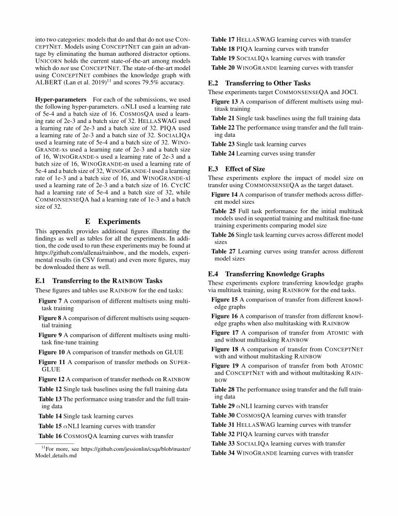
Figure 11 A comparison of transfer methods on SUPER-GLUE

Figure 12 A comparison of transfer methods on RAINBOW

Table 12 Single task baselines using the full training data

Table 13 The performance using transfer and the full train-ing data

Table 14 Single task learning curves

Table 15 αNLI learning curves with transfer

Table 16 COSMOSQA learning curves with transfer

11For more, see https://github.com/jessionlin/csqa/blob/master/Model details.md

Table 17 HELLASWAG learning curves with transferTable 18 PIQA learning curves with transferTable 19 SOCIALIQA learning curves with transferTable 20 WINOGRANDE learning curves with transfer

E.2 Transferring to Other TasksThese experiments target COMMONSENSEQA and JOCI.Figure 13 A comparison of different multisets using mul-

titask trainingTable 21 Single task baselines using the full training dataTable 22 The performance using transfer and the full train-

ing dataTable 23 Single task learning curvesTable 24 Learning curves using transfer

E.3 Effect of SizeThese experiments explore the impact of model size ontransfer using COMMONSENSEQA as the target dataset.

Figure 14 A comparison of transfer methods across differ-ent model sizes

Table 25 Full task performance for the initial multitaskmodels used in sequential training and multitask fine-tunetraining experiments comparing model size

Table 26 Single task learning curves across different modelsizes

Table 27 Learning curves using transfer across differentmodel sizes

E.4 Transferring Knowledge GraphsThese experiments explore transferring knowledge graphsvia multitask training, using RAINBOW for the end tasks.

Figure 15 A comparison of transfer from different knowl-edge graphs

Figure 16 A comparison of transfer from different knowl-edge graphs when also multitasking with RAINBOW

Figure 17 A comparison of transfer from ATOMIC withand without multitasking RAINBOW

Figure 18 A comparison of transfer from CONCEPTNETwith and without multitasking RAINBOW

Figure 19 A comparison of transfer from both ATOMICand CONCEPTNET with and without multitasking RAIN-BOW

Table 28 The performance using transfer and the full train-ing data

Table 29 αNLI learning curves with transferTable 30 COSMOSQA learning curves with transferTable 31 HELLASWAG learning curves with transferTable 32 PIQA learning curves with transferTable 33 SOCIALIQA learning curves with transferTable 34 WINOGRANDE learning curves with transfer

Figure 7: A comparison of multisets for transfer to the RAINBOW tasks using multitask training with T5-LARGE. Performanceis dev accuracy.

Figure 8: A comparison of multisets for transfer to the RAINBOW tasks using sequential training with T5-LARGE. Performanceis dev accuracy.

Figure 9: A comparison of multisets for transfer to the RAINBOW tasks using multitask fine-tune training with T5-LARGE.Performance is dev accuracy.

Figure 10: A comparison of methods for transferring GLUE to the RAINBOW tasks with T5-LARGE. Performance is devaccuracy.

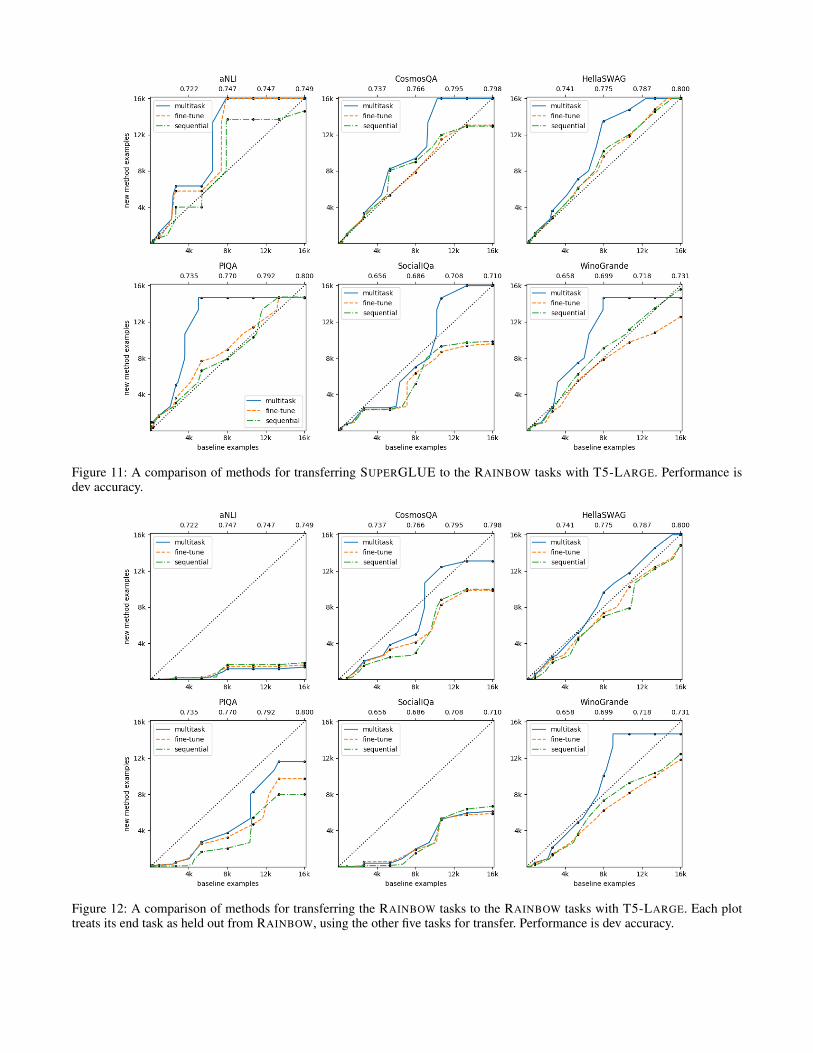
Figure 11: A comparison of methods for transferring SUPERGLUE to the RAINBOW tasks with T5-LARGE. Performance isdev accuracy.

Figure 12: A comparison of methods for transferring the RAINBOW tasks to the RAINBOW tasks with T5-LARGE. Each plottreats its end task as held out from RAINBOW, using the other five tasks for transfer. Performance is dev accuracy.

Taskmodel αNLI COSMOSQA HELLASWAG PIQA SOCIALIQA WINOGRANDE

large 77.8 81.9 82.8 80.2 73.8 77.0

Table 12: Single task baselines using the full training data.

Taskmultiset transfer αNLI COSMOSQA HELLASWAG PIQA SOCIALIQA WINOGRANDE

GLUEfine-tune 78.5 82.4 82.9 80.1 74.3 78.4multitask 77.2 80.8 81.8 77.6 74.7 76.0sequential 78.5 81.4 82.3 80.8 74.3 77.9

RAINBOWfine-tune 79.2 82.6 83.1 82.2 75.2 78.2multitask 78.4 81.1 81.3 80.7 74.8 72.1sequential 79.5 83.2 83.0 82.2 75.5 78.7

SUPERGLUEfine-tune 78.5 81.7 82.8 80.0 74.7 78.5multitask 77.7 78.9 80.5 70.7 72.3 69.8sequential 79.1 82.2 82.5 80.7 74.6 77.6

Table 13: The performance using transfer and the full training data.

Sizetask 4 10 30 91 280 865 2667 5334 8000 10667 13334 16000

αNLI 49.2 53.1 54.8 61.1 65.6 68.4 72.3 72.1 76.1 73.4 74.4 74.9COSMOSQA 24.6 31.0 26.2 31.9 43.0 61.3 71.7 75.6 76.6 79.2 80.0 79.6HELLASWAG 24.6 26.6 26.0 32.6 48.6 64.6 72.5 75.8 77.5 78.2 79.2 80.0PIQA 50.1 50.7 51.7 52.8 52.7 59.8 70.7 76.3 77.0 78.4 80.0 80.0SOCIALIQA 33.6 34.7 34.4 34.7 35.3 54.0 66.4 64.7 68.6 70.6 70.9 71.0WINOGRANDE 50.1 50.7 52.9 50.7 51.1 57.9 64.2 67.4 69.9 71.4 72.2 73.1

Table 14: Learning curves for the single task baselines.

Sizemultiset transfer 4 10 30 91 280 865 2667 5334 8000 10667 13334 16000

GLUEfine-tune 49.2 53.7 60.1 61.9 66.2 69.2 72.6 72.7 75.4 73.2 74.2 74.6multitask 49.2 53.3 59.3 61.7 66.1 69.5 72.3 72.4 74.5 73.2 74.2 74.3sequential 49.1 57.1 63.1 63.8 67.4 70.0 72.8 73.4 75.8 74.3 74.3 75.4

RAINBOWfine-tune 61.0 63.4 69.6 71.3 72.6 73.9 76.6 75.8 76.7 75.8 76.4 76.7multitask 61.9 62.9 69.6 71.4 73.0 74.3 76.4 76.7 76.9 76.8 77.5 77.2sequential 61.4 65.3 70.9 71.0 73.6 73.8 75.8 75.7 76.6 76.6 76.6 76.5

SUPERGLUEfine-tune 49.1 57.0 59.9 63.6 66.1 69.1 71.3 71.9 75.3 73.6 73.3 74.5multitask 49.1 57.0 59.5 63.7 65.5 67.9 71.3 71.6 74.3 72.8 72.7 74.5sequential 49.2 61.5 62.6 64.8 66.3 70.2 72.2 72.3 76.1 73.6 74.0 75.2

Table 15: Learning curves on αNLI using transfer.





Table 16: Learning curves on COSMOSQA using transfer.





Table 17: Learning curves on HELLASWAG using transfer.





Table 18: Learning curves on PIQA using transfer.





Table 19: Learning curves on SOCIALIQA using transfer.





Table 20: Learning curves on WINOGRANDE using transfer.

Figure 13: A comparison of transfer from different multisets to COMMONSENSEQA and JOCI with T5-LARGE via multitasktraining. Performance is dev accuracy.

Taskmodel COMMONSENSEQA JOCI

large 71.6 58.0

Table 21: Single task baselines using the full training data.

Taskmultiset COMMONSENSEQA JOCI

GLUE 70.8 57.8RAINBOW 72.6 57.5SUPERGLUE 70.5 58.3

Table 22: The performance on COMMONSENSEQA and JOCI using transfer via multitask training.

Sizetask 4 10 30 91 280 865 2667 5334 8000 9741 10667 13334 16000

COMMONSENSEQA 19.9 35.1 45.6 53.6 58.3 63.2 66.3 70.8 71.4 72.0 – – –JOCI 21.8 24.6 29.3 28.8 43.3 48.7 52.0 53.5 55.4 – 55.3 56.0 57.4

Table 23: Learning curves for the single task baselines on COMMONSENSEQA and JOCI.

Sizetask multiset 4 10 30 91 280 865 2667 5334 8000 9741 10667 13334 16000

COMMON-SENSEQA

GLUE 21.5 31.0 42.3 53.5 57.7 62.9 66.3 69.5 70.4 71.1 – – –RAINBOW 41.7 63.2 63.7 63.9 65.7 66.7 68.3 71.8 72.1 73.0 – – –SUPERGLUE 20.7 35.0 42.0 54.1 57.9 63.3 65.9 69.0 70.7 70.7 – – –

JOCIGLUE 22.4 24.7 30.5 29.0 43.4 50.2 52.1 54.4 54.9 – 55.4 56.1 57.2RAINBOW 21.8 24.2 30.2 30.3 42.6 48.5 52.0 53.6 54.4 – 55.4 55.0 56.7SUPERGLUE 21.9 24.5 30.2 29.2 43.1 50.4 52.4 53.6 55.8 – 55.4 56.0 56.5

Table 24: Learning curves using multitask training on COMMONSENSEQA and JOCI.

Figure 14: A comparison of transfer methods from RAINBOW to COMMONSENSEQA across model sizes with T5-SMALL,T5-BASE, and T5-LARGE. Performance is dev accuracy.

Taskmodel αNLI COSMOSQA HELLASWAG PIQA SOCIALIQA WINOGRANDE

base 65.3 72.8 56.2 73.3 66.1 61.8large 76.2 81.1 81.3 80.7 74.5 72.1small 57.0 44.5 31.8 54.6 46.8 52.4

Table 25: Full task performance for UNICORN on RAINBOW after multitask training and before training on the target dataset(COMMONSENSEQA) across different model sizes.

Sizemodel 4 10 30 91 280 865 2667 5334 8000 9741

base 29.1 30.6 29.2 41.5 46.4 49.7 55.1 59.3 60.9 60.8large 19.9 35.1 45.6 53.6 58.3 63.2 66.3 70.8 71.4 72.0small 20.5 23.1 19.2 26.4 25.4 24.9 32.0 36.8 40.0 42.1

Table 26: Learning curves for single task baselines on COMMONSENSEQA at different model sizes.

Sizemodel transfer 4 10 30 91 280 865 2667 5334 8000 9741

basefine-tune 37.5 47.1 46.5 47.9 49.2 51.0 55.1 59.2 59.9 60.6multitask 36.4 47.7 46.9 48.9 49.2 52.7 55.4 58.3 59.5 60.0sequential 38.4 45.4 45.6 48.1 50.2 52.7 56.1 59.7 61.6 61.6

largefine-tune 47.4 64.0 63.8 63.0 65.7 66.5 68.8 71.6 71.8 72.6multitask 41.7 63.2 63.7 63.9 65.7 66.7 68.3 71.8 72.1 73.0sequential 59.5 63.3 63.0 64.0 65.9 68.1 69.8 72.9 73.1 72.6

smallfine-tune 26.3 30.9 30.3 27.7 29.7 31.1 33.5 36.6 37.8 40.2multitask 26.3 30.7 29.7 28.9 29.9 31.7 33.0 36.6 40.5 40.1sequential 25.1 28.7 29.1 27.8 29.8 31.0 32.7 38.0 39.3 41.0

Table 27: Learning curves for UNICORN on COMMONSENSEQA at different model sizes, with different transfer approaches.

Figure 15: A comparison of transfer from different knowledge graphs to the RAINBOW tasks using multitask training. Perfor-mance is dev accuracy.

Figure 16: A comparison of transfer from different knowledge graphs and RAINBOW to the RAINBOW tasks using multitasktraining. Performance is dev accuracy.

Figure 17: A comparison of transfer from ATOMIC to the RAINBOW tasks via multitask training when also and not alsomultitasking with RAINBOW.

Figure 18: A comparison of transfer from CONCEPTNET to the RAINBOW tasks via multitask training when also and not alsomultitasking with RAINBOW.

Figure 19: A comparison of transfer from both ATOMIC and CONCEPTNET to the RAINBOW tasks via multitask training whenalso and not also multitasking with RAINBOW.

Taskmultiset knowledge direction αNLI COSMOSQA HELLASWAG PIQA SOCIALIQA WINOGRANDE

NONE

ATOMICbackward 78.3 81.8 82.5 79.5 74.3 76.9bidirectional 77.9 81.0 82.8 79.3 75.0 78.2forward 77.7 81.0 82.4 79.9 74.4 76.8

CONCEPTNETbackward 78.0 81.8 82.5 79.4 74.3 76.3bidirectional 77.8 81.5 82.3 80.5 74.1 76.3forward 77.5 81.6 82.1 80.0 73.7 76.2

BOTHbackward 78.0 81.2 82.4 81.1 74.4 75.7bidirectional 77.6 81.0 82.6 80.1 74.7 76.4forward 77.5 81.8 82.7 79.8 74.8 76.6

RAINBOW

ATOMICbackward 78.3 81.4 81.3 80.5 75.0 73.2bidirectional 77.7 81.4 81.2 80.4 74.9 71.5forward 77.9 81.3 81.6 80.4 75.0 73.6

CONCEPTNETbackward 78.7 81.8 81.6 81.3 75.0 73.5bidirectional 78.8 80.6 81.5 81.0 74.7 72.9forward 78.3 81.6 81.3 80.6 75.5 73.4

BOTHbackward 77.1 80.9 81.6 81.2 74.3 71.6bidirectional 76.9 81.4 81.0 80.3 75.0 72.2forward 77.7 81.9 81.7 80.8 74.8 72.1

Table 28: The performance when transferring different knowledge graphs to RAINBOW with multitask training using the fulltraining data.

Sizemultiset knowledge 4 10 30 91 280 865 2667 5334 8000 10667 13334 16000

NONEATOMIC 49.3 52.3 54.6 61.6 65.8 68.5 71.6 72.5 75.3 73.4 74.1 74.8CONCEPTNET 49.2 54.6 53.5 60.2 65.5 68.6 72.2 71.7 74.4 73.1 74.0 74.9BOTH 49.3 54.0 52.9 59.6 66.3 68.5 72.4 71.6 74.7 73.6 74.0 75.0

RAINBOWATOMIC 55.0 67.0 73.0 72.0 73.8 74.9 76.2 76.4 76.6 76.8 76.6 77.0CONCEPTNET 56.7 66.4 64.5 72.7 75.2 75.1 76.2 76.4 77.1 76.3 76.4 76.6BOTH 58.3 64.7 65.4 72.1 73.2 74.5 76.2 76.0 76.6 76.6 77.0 76.7

Table 29: Learning curves on αNLI using transfer from knowledge graphs via multitask training.




Table 30: Learning curves on COSMOSQA using transfer from knowledge graphs via multitask training.




Table 31: Learning curves on HELLASWAG using transfer from knowledge graphs via multitask training.




Table 32: Learning curves on PIQA using transfer from knowledge graphs via multitask training.




Table 33: Learning curves on SOCIALIQA using transfer from knowledge graphs via multitask training.




Table 34: Learning curves on WINOGRANDE using transfer from knowledge graphs via multitask training.

unicorn on rainbow: a universal commonsense reasoning

Documents