IntroductionUnico is a cross-platform graphical user interface (GUI) running on Windows, Linux and Mac OS for the demonstration boards ofMEMS sensors such as accelerometers, gyroscopes, magnetometers and environmental sensors available in theSTMicroelectronics portfolio.

Unico interacts with all the MEMS demonstration boards supported by the STEVAL-MKI109V3 (Professional MEMS tool)motherboard and allows a quick and easy setup of the sensors, as well as the complete configuration of all the registers and theadvanced features embedded in the digital output devices. The software visualizes the output of the sensors in both graphicaland numeric format and allows the user to save or generally manage data coming from the device.

This user manual describes all the functions of the Unico GUI. For details regarding the features of each sensor, please refer tothe related device datasheet.

Unico GUI

UM1049

User manual

UM1049 - Rev 6 - January 2019For further information contact your local STMicroelectronics sales office.

www.st.com

1 PC system requirements

Unico software has been designed to operate with Microsoft® Windows platforms, Linux platforms, and Mac OS Xplatforms.

1.1 Windows platformsA virtual COM driver must be installed to allow communication with the motherboard. Please refer to theProfessional MEMS tool board user manual for the installation.The package “Microsoft Visual C++ 2010 Redistributable Package (x86)” needs to be installed to be able to runUnico on Windows; it can be downloaded from Microsoft Download Center.To install the Unico GUI, launch the “Setup_Unico.exe” file included in the package and follow the instructionswhich appear on the screen. When the software is installed, you can run it from: “Start > STMicroelectronics >Unico > Unico.exe”

1.2 Linux platformsFor Linux Debian-based distributions, a .deb package is provided in the package.On Ubuntu, you can install the .deb package by opening a terminal and writing the following command:sudo dpkg -i unico.debIf the installation fails for any missing dependent library, it is necessary to install the missing library beforeproceeding with the Unico installation:sudo apt-get install <missing_library_name>sudo dpkg -i unico.debNote: Unico dynamically links to the Qt5 libraries, so they need to be installed on your system to make it work.After the installation has been completed, the executable file (“unico”) will be stored in the /usr/local/bin folder. Youmay need to change the permission of the “unico” executable file with the following command:sudo chmod +x /usr/local/bin/unicoTo run the Unico software, just type:/usr/local/bin/unicoNote: The current version of Unico is designed to work on Ubuntu 14.04 LTS, although it should be possible toinstall and run it on other Debian-based distributions after having installed all the dependencies required.

1.3 Mac OS X platformsFor Mac OS, a DMG file (unico.dmg) is provided in the package.To install Unico:1. Double-click the DMG file to open it up. A finder window containing the unico application will appear.2. Drag and drop the unico application into your “Applications” directory in order to install Unico on your Mac.To run Unico, just click on the unico application under “Applications”.

UM1049PC system requirements

UM1049 - Rev 6 page 2/34

2 Unico graphical user interface

After launching the Unico GUI, a launcher window will appear, as shown in Figure 1. Unico launcher. The GUIshows the list of adapter boards supported by the current release, grouped according to the device type.

Figure 1. Unico launcher

Choose the board currently in use from the list and then click on the button “Select Device”. The main window willappear after a few seconds (Figure 2. Unico main window).In the launcher window, it is also possible to get a brief description of the selected sensor by clicking on the“Description” button.The GUI can automatically detect the port where the board is connected. However, if the user has noadministrator rights, or in case of Bluetooth connection, the port selection must be done manually, unchecking the“Automatic Port Detection” check-box. For further information on how to detect the port manually refer toSection 4 Port detection.On Linux, permissions on the serial port could be required to establish the connection. If so, the GUI will suggestthe command to be executed (for instance: sudo chmod 666 ttyACM0) and will open a terminal to run thecommand.Unchecking the "Communication with the motherboard" checkbox, it is possible to run Unico offline. In this case,the GUI cannot communicate with the sensor, so its functionality is limited to the features which do not requireinteraction with the motherboard.

UM1049Unico graphical user interface

UM1049 - Rev 6 page 3/34

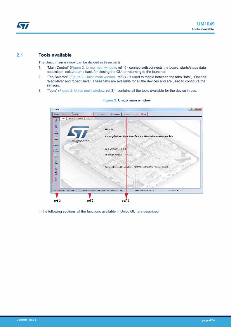
2.1 Tools availableThe Unico main window can be divided in three parts:1. “Main Control” (Figure 2. Unico main window, ref 1) - connects/disconnects the board, starts/stops data

acquisition, exits/returns back for closing the GUI or returning to the launcher.2. “Tab Selector” (Figure 2. Unico main window, ref 2) - is used to toggle between the tabs “Info”, “Options”,

“Registers” and “Load/Save”. These tabs are available for all the devices and are used to configure thesensors.

3. “Tools” (Figure 2. Unico main window, ref 3) - contains all the tools available for the device in use.

Figure 2. Unico main window

In the following sections all the functions available in Unico GUI are described.

UM1049Tools available

UM1049 - Rev 6 page 4/34

2.2 Options tabThe options tab allows the user to control the main parameters of the selected sensor. The content of the tabdepends on the sensor chosen. The following parameters refer to a 3-axis digital accelerometer plus a 3-axisdigital magnetometer:1. Easy Configuration: Turns on the device and sets a default configuration (Figure 3. Options tab, ref 1).2. Accelerometer full scale (FS): sets the maximum acceleration value measurable by the device

(Figure 3. Options tab, ref 2).3. Accelerometer operating mode (OM): selects the operating mode (e.g. normal mode or power-down mode)

(Figure 3. Options tab, ref 3).4. Accelerometer’s high-pass filter (HP): activates the high-pass filter of the accelerometer and selects the

cutoff frequency (Figure 3. Options tab, ref 4).5. Magnetometer full scale (FS): sets the maximum magnetic field measurable by the device (Figure 3. Options

tab, ref 5).6. Magnetometer data rate (ODR): sets the magnetometer output data rate (Figure 3. Options tab, ref 6).7. Magnetometer operating mode: selects the operating mode of the magnetometer (e.g. normal

measurement) (Figure 3. Options tab, ref 7).

Figure 3. Options tab

UM1049Options tab

UM1049 - Rev 6 page 5/34

2.3 Register setup tabThe register setup tab shown in Figure 4. Register setup tab allows reading and writing the content of theregisters embedded in the MEMS sensor mounted on the demonstration kit. The tab is divided in three sections:1. “General” (Figure 4. Register setup tab, ref 1) - provides access to the registers which control the main

settings of the device. This section contains control registers, registers to manage the interrupt generation,and so on. It is possible to read and write the contents of each register. To read the default value for a givenregister, press the “Default” button (in this case no data is written in the register, to do this please click the“Write” button).

2. “Direct communication” (Figure 4. Register setup tab, ref 2) - provides access to any register in the device.To read a generic register, insert the address value in the “Register Address” text box, then click on the“Read” button. The retrieved content of the register is displayed in the “Register Value” field. As with writingto a register, the user must specify the address and the data to be written inside the fields marked “RegisterAddress” and “Register Value” respectively, then press the “Write” button. “Read All”, “Write All”, and “DefaultAll” perform the same functions but for all the registers at the same time.

3. “Easy Configuration” - this button provides the user the possibility to choose a default configuration, allowingan easy start. When pressed, the sensor register is automatically configured with the default configuration(Figure 4. Register setup tab ref 3).

Figure 4. Register setup tab

UM1049Register setup tab

UM1049 - Rev 6 page 6/34

2.4 Load/Save tabThis tab allows the user to save a stream of sensor output data in a text file, available for possible post-processing (Figure 5. Load/Save tab, ref 1). It is possible to select which data must be stored. The “Browse”button is used to select the folder and insert the file name, then the “Start” and “Stop” buttons define theacquisition period.It is also possible to save the current register configuration by clicking on the “Save” button. The configurationsaved can be loaded at any time by clicking on the “Load” button (Figure 5. Load/Save tab, ref 2).

Figure 5. Load/Save tab

UM1049Load/Save tab

UM1049 - Rev 6 page 7/34

2.5 Bars toolThe bars tool (Figure 6. Bars tool) displays the data measured by the sensor in a bar chart format. For instance, inthe case of a 6-axis module, the accelerations along the X, Y, and Z axes correspond respectively to the red,green, and blue bars. The same colors are used to represent the magnetic values along X, Y, and Z axes.The height of each bar is determined by the amplitude of the signal measured by the sensor along the relatedaxis. The full scale of the graph depends on the configuration and can be changed through both the option tab(Figure 3. Options tab, ref 2, ref 6) and the register tab (Figure 4. Register setup tab, ref 1, ref 2).

Figure 6. Bars tool

UM1049Bars tool

UM1049 - Rev 6 page 8/34

2.6 Plot toolThe plot tool shows the evolution of the output over time. Figure 7. Plot tool shows the sequence of theaccelerometer and magnetometer samples which have been measured by the 6-axis module mounted on thedemonstration kit.If the selected device contains just the accelerometer, the magnetic part is hidden. In the case of gyroscopes, theplot shows the angular rates.

Figure 7. Plot tool

UM1049Plot tool

UM1049 - Rev 6 page 9/34

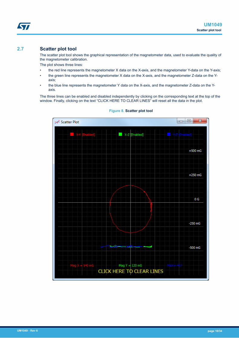
2.7 Scatter plot toolThe scatter plot tool shows the graphical representation of the magnetometer data, used to evaluate the quality ofthe magnetometer calibration.The plot shows three lines:• the red line represents the magnetometer X data on the X-axis, and the magnetometer Y-data on the Y-axis;• the green line represents the magnetometer X data on the X-axis, and the magnetometer Z-data on the Y-

axis;• the blue line represents the magnetometer Y data on the X-axis, and the magnetometer Z-data on the Y-

axis.

The three lines can be enabled and disabled independently by clicking on the corresponding text at the top of thewindow. Finally, clicking on the text “CLICK HERE TO CLEAR LINES” will reset all the data in the plot.

Figure 8. Scatter plot tool

UM1049Scatter plot tool

UM1049 - Rev 6 page 10/34

2.8 Data toolThe data tool (Figure 9. Data tool) shows the output values measured by the sensor connected to thedemonstration board. For a 6-axis module, the data is divided in the following sections:1. “LSB Data” (Figure 9. Data tool, ref 1) - displays acceleration and magnetic data provided by the sensor in

LSB (no sensitivity is applied).2. “Physical Data” (Figure 9. Data tool, ref 2) - represents the acceleration/magnetic data measured by the

sensor, expressed in the related unit of measurements (taking account of the sensitivity).3. “Azimuth” (Figure 9. Data tool, ref 3) - displays the azimuth calculated using the magnetic field data.4. “Angle” (Figure 9. Data tool, ref 4) - returns the tilt angle, 7 degrees.

Figure 9. Data tool

UM1049Data tool

UM1049 - Rev 6 page 11/34

2.9 Interrupt toolThe interrupt tool (Figure 10. Interrupt tool) allows evaluating the interrupt generation features of the MEMSsensor. In this window it is possible to configure the characteristics of the inertial events that must be recognizedby the device, and to visualize (in real time) the evolution of the two interrupt lines.The GUI provides the access to the interrupt registers (such as: INT_CFG, INT_SRC, THS and duration) whichallow the configuration of the two independent interrupt sources of the device (Figure 10. Interrupt tool, ref 2). Thelabels located at the bottom of the graph (Figure 10. Interrupt tool, ref 1) show threshold and duration values.Finally, two buttons per interrupt line are available in the tool, in order to easily set the recommendedconfiguration for free-fall and wake-up detection (Figure 10. Interrupt tool, ref 3).

Figure 10. Interrupt tool

UM1049Interrupt tool

UM1049 - Rev 6 page 12/34

2.10 Compass toolThe compass tool shows an example of compass application (Figure 11. Compass tool, ref 3), which can beimplemented using a 6-axis module (3-axis accelerometer and 3-axis magnetometer).The algorithm uses the magnetometer data to measure the Earth’s magnetic field, and the accelerometer data tocompensate the board inclination. Rotating the board, the GUI shows the heading of the compass(Figure 11. Compass tool, ref 1).The performance of the compass is related to the configuration used. So, the GUI shows the current configurationand the recommended configuration (accelerometer and magnetometer ODR, Figure 11. Compass tool, ref 2).Before using the compass demo, the system must be calibrated by moving the board randomly for a few seconds;the quality of the calibration step is indicated by a colored bar (Figure 11. Compass tool, ref 4). A green coloredbar means that the quality of the calibration is optimal.

Figure 11. Compass tool

UM1049Compass tool

UM1049 - Rev 6 page 13/34

2.11 FIFO toolThe FIFO tool can be used to test the first-in first-out data buffer embedded in the device, when this feature issupported by the sensor (see the device datasheet for more details).By using the buttons available in the window (Figure 12. FIFO tool, ref 1), the FIFO can be configured in all thesupported modes (e.g. Bypass, FIFO, Stream, Stream-to-FIFO).The GUI shows the values of the X, Y, Z data stored in the 32-byte deep FIFO buffer, indicating both numericaldata (Figure 12. FIFO tool, ref 4) and the corresponding graph (Figure 12. FIFO tool, ref 2).Finally, it allows users to save the data in a text file, which can be used for post-processing (Figure 12. FIFO tool,ref 3).

Figure 12. FIFO tool

UM1049FIFO tool

UM1049 - Rev 6 page 14/34

2.12 State machine toolThe Finite State Machine tool allows the user to configure the state machines and test their functionality.In the top part of the Finite State Machine tool main window, the user can select which state machine is selected(the selection is applied in both the Configuration tab and the Debug tab). It is also possible to configure the FSMODR (data rate) and the long counter parameters. Finally, a converter from float32 to float16 format and viceversais available. The converter is used to generate the values to be set in the threshold resources in the Variable DataSection.Three different tabs are available for this tool:• Configuration (Section 2.12.1 Configuration tab) - allows setting a configuration for the state machines;• Interrupt (Section 2.12.2 Interrupt tab) - shows a plot with accelerometer and gyroscope XYZ data in [g] and

[dps], interrupt lines and state machine output register information;• Debug (Section 2.12.3 Debug tab) - injects log file data in the device in order to check the functionality of the

configured programs

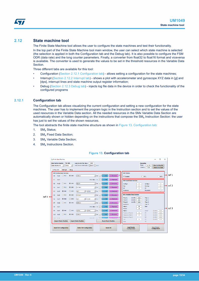
2.12.1 Configuration tabThe Configuration tab allows visualizing the current configuration and setting a new configuration for the statemachines. The user has to implement the program logic in the Instruction section and to set the values of theused resources in the Variable Data section. All the needed resources in the SMx Variable Data Section areautomatically shown or hidden depending on the instructions that compose the SMx Instruction Section: the userhas just to set the values of the shown resources.The tool abstracts the finite state machine structure as shown in Figure 13. Configuration tab:1. SMx Status;2. SMx Fixed Data Section;3. SMx Variable Data Section;4. SMx Instructions Section.

Figure 13. Configuration tab

UM1049State machine tool

UM1049 - Rev 6 page 15/34

2.12.2 Interrupt tabThe Interrupt tab shows the accelerometer and gyroscope data in [g] and [dps] format, the evolution of theinterrupt lines and the state machine interrupts information. It helps the user to check the program functionalities.The interrupt tab is divided in two parts as shown in Figure 14. Interrupt tab:1. Signal plots;2. State machine interrupts status.

Figure 14. Interrupt tab

In the State Machine Interrupts groupbox, a graphic green LED is turned on for ~300 msec each time thecorresponding state machine interrupt source bit is set to ‘1’. It is also possible to read the corresponding statemachine OUT_Sx register by clicking on the corresponding “Read” button.

UM1049State machine tool

UM1049 - Rev 6 page 16/34

2.12.3 Debug tabThe Debug tab shows a graphic configuration of the current program set in the selected state machine and allowsdebugging, sample by sample, after loading an input data pattern. It is used to check the state machinefunctionality in order to help the user to validate the program. It is composed of three parts:1. State machine flow;2. Debug commands;3. Output results.When the debug mode is enabled, the current state is highlighted and it is automatically updated based on theinjected sample and program behavior. The tool provides the possibility to inject one or more samples at a time:each time a sample is injected, a new row containing the updated values of the state machine resources is addedin the results of the output table.

Figure 15. Debug tab

UM1049State machine tool

UM1049 - Rev 6 page 17/34

2.13 Machine Learning Core toolThe Machine Learning Core (MLC) tool allows the user to configure a machine learning core which is embeddedin some devices. Two different tabs are available for this tool:• Data Patterns (Figure 16. MLC Data Patterns tab) – allows managing the data patterns to be used and

assigning a label to each data pattern loaded.• Configuration (Figure 17. MLC Configuration tab) – allows setting a configuration for the machine learning

core.

2.13.1 Data Patterns tabThe Data Patterns tab allows managing the data patterns to be used for the machine learning processing. Thedata patterns which are possible to load must have the same data format as the log files generated by Unico inthe Load/Save tab. The unit of measurement for the data are ‘mg’ for the accelerometer and ‘dps’ for thegyroscope.When a new data pattern is loaded, an expected result must be assigned, which is the label for the machinelearning processing.

Figure 16. MLC Data Patterns tab

UM1049Machine Learning Core tool

UM1049 - Rev 6 page 18/34

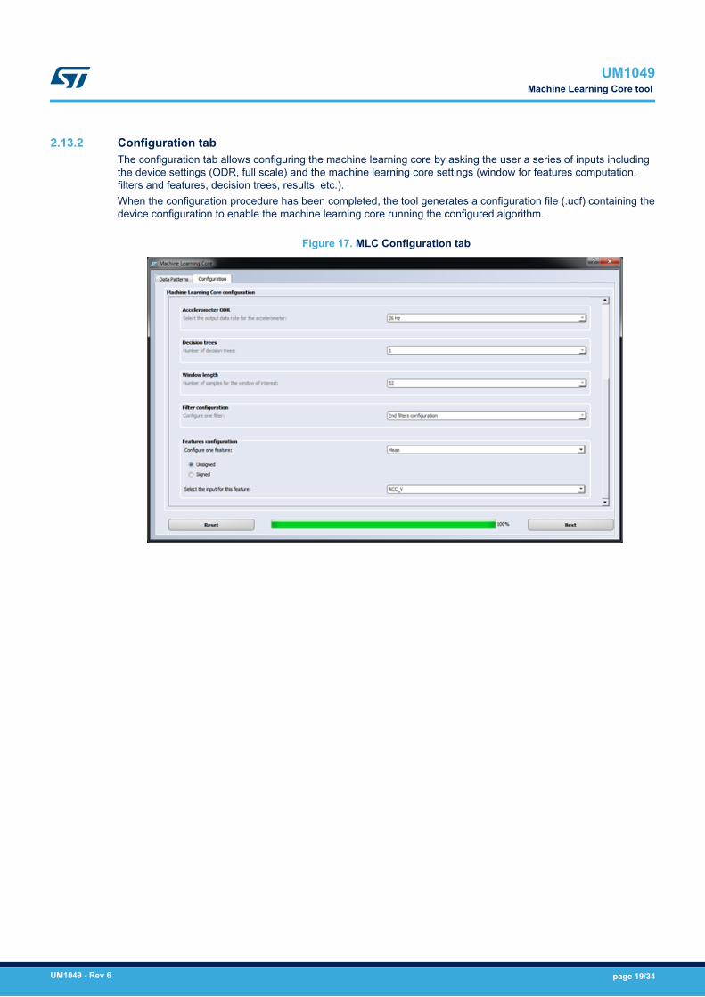
2.13.2 Configuration tabThe configuration tab allows configuring the machine learning core by asking the user a series of inputs includingthe device settings (ODR, full scale) and the machine learning core settings (window for features computation,filters and features, decision trees, results, etc.).When the configuration procedure has been completed, the tool generates a configuration file (.ucf) containing thedevice configuration to enable the machine learning core running the configured algorithm.

Figure 17. MLC Configuration tab

UM1049Machine Learning Core tool

UM1049 - Rev 6 page 19/34

2.14 Click toolThe click tool (Figure 18. Click tool) allows evaluating the click or double-click function of the MEMS sensor. Inthis window it is possible to configure the device for single-click and double-click detection and visualize (in realtime) the evolution of the interrupt line.This tool is available only for the devices which integrates the click/double-click function.By clicking the buttons “Set Single Click” (Figure 18. Click tool, ref 1) or “Set Double Click” (Figure 18. Click tool,ref 2), a default configuration for single-click or double-click detection will be loaded. After loading theconfiguration, a green light will appear when the single or double click has been recognized.It is also possible to change the register configuration by setting different values in the interrupt registers shown inthe tool (Figure 18. Click tool, ref 3).

Figure 18. Click tool

UM1049Click tool

UM1049 - Rev 6 page 20/34

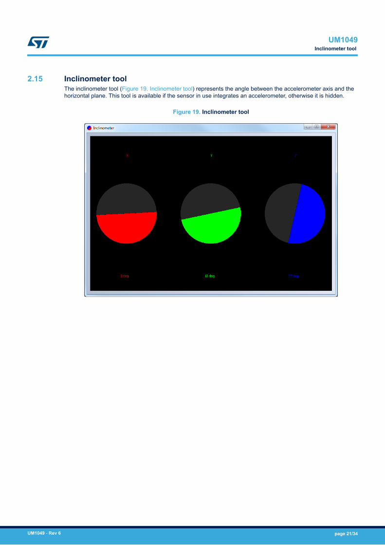
2.15 Inclinometer toolThe inclinometer tool (Figure 19. Inclinometer tool) represents the angle between the accelerometer axis and thehorizontal plane. This tool is available if the sensor in use integrates an accelerometer, otherwise it is hidden.

Figure 19. Inclinometer tool

UM1049Inclinometer tool

UM1049 - Rev 6 page 21/34

2.16 6D toolThe 6D tool (Figure 20. 6D tool) provides an example of how to use the “6D position” function.In this tool it is possible to configure the interrupt for 6D recognition by clicking the button “Set 6D” (Figure 20. 6Dtool, ref 1). After loading the configuration, the teapot will be oriented depending on the 6D position detected(Figure 20. 6D tool, ref 2). The window also shows (in real time) the evolution of the interrupt line.It is also possible to change the register configuration by setting different values in the interrupt registers shown inthe tool (Figure 20. 6D tool, ref 2).

Figure 20. 6D tool

UM10496D tool

UM1049 - Rev 6 page 22/34

2.17 FFT toolThe FFT tool (Figure 21. FFT tool) shows the Fast Fourier Transform of the output data.The window shows time-domain plot (Figure 21. FFT tool, ref 1), and the frequency-domain plot for each axis(Figure 21. FFT tool, ref 2).The FFT is performed on the latest 128 samples of the time-domain waveform, so the spectrum in the frequencydomain will be divided in 64 frequencies (from 0 to ODR/2 Hz).The frequency domain plots show the module of the Fourier transform of each axis, expressed in g for theaccelerometer and dps for the gyroscope.

Figure 21. FFT tool

UM1049FFT tool

UM1049 - Rev 6 page 23/34

2.18 Pedometer toolThe pedometer tool can be used to configure and test the pedometer embedded in the device when this feature issupported by the sensor (see the device datasheet for more details).Three different tabs are available for this tool:• Configuration / output tab (see Section 2.18.1 Configuration / Output tab): it allows fast-configuring the

pedometer with its default configuration.• Debug / Data Injection tab (see Section 2.18.2 Debug / Data Injection tab): it is used to load a data

pattern into the device in order to test (offline) the pedometer on the pattern itself.• Regression Tool tab (see Section 2.18.3 Regression Tool tab): it allows finding an optimal configuration

on the base of a predefined dataset.

2.18.1 Configuration / Output tabThe Configuration / Output tab (Figure 22. Configuration / Output tab) allows fast-configuring the pedometer. Inthis window it is possible to visualize in real-time the evolution of both the accelerometer signal and the twointerrupt lines (Figure 22. Configuration / Output tab, ref 1) and to read the output pedometer step count(Figure 22. Configuration / Output tab, ref 3).One button is available in the tool in order to easily enable and configure the pedometer with its defaultconfiguration (Figure 22. Configuration / Output tab, ref 4). The GUI also allows directly accessing the pedometerregisters (such as PEDO_CMD_REG, PEDO_DEB_STEPS_CONF, PEDO_SC_DELTAT_L,PEDO_SC_DELTAT_H) in order to set a user-defined pedometer configuration (Figure 22. Configuration / Outputtab, ref 2).

Figure 22. Configuration / Output tab

UM1049Pedometer tool

UM1049 - Rev 6 page 24/34

2.18.2 Debug / Data Injection tabThe Debug / Data Injection tab (Figure 23. Debug / Data Injection tab) is used to load a data pattern into thedevice and run the pedometer logic on the pattern itself (offline post-processing).On the left side of the GUI a three button toolbar is available for loading a data pattern in the GUI. Pedometerconfiguration can be loaded from the .ucf file; it is also possible to fast-configure the pedometer in its defaultconfiguration by clicking on the “Pedometer Easy Configuration” button (Figure 23. Debug / Data Injection tab, ref1). The device enters the debug mode right after the data pattern has been loaded.On the top of the GUI, a toolbar is available to control the data injection (Figure 23. Debug / Data Injection tab, ref2), which can be applied with the maximum level of flexibility:• “Next” button is used to load one sample in the pedometer;• “All Next” button is used to load sample-by-sample the full data pattern in the pedometer;• “Run” button is used to load the entire pattern in the pedometer, displaying the final result only;• “N Next” button allows loading the indicated number of samples in the pedometer, displaying all the samples;• “N Run” button allows loading the indicated number of samples, displaying the final result only;• “Stop” button allows stopping the current debug session. If the button ‘All Next’ or ‘Run’ was pressed, the

‘Stop’ button changes into ‘Pause’ button, which allows pausing the current debug session with thepossibility to resume it. When the debug session is paused, the ‘Stop’ button changes again into ‘Stop’button, allowing the possibility to stop the current debug session. After that, another debug session can belaunched (the data pattern must be reloaded).

During a debug session, the current status (sample loaded and output number of steps) is displayed in the centralpart of the GUI (Figure 23. Debug / Data Injection tab, ref 3). A dedicated button is also available in order toexport the results of the debug session in TSV format.

Figure 23. Debug / Data Injection tab

UM1049Pedometer tool

UM1049 - Rev 6 page 25/34

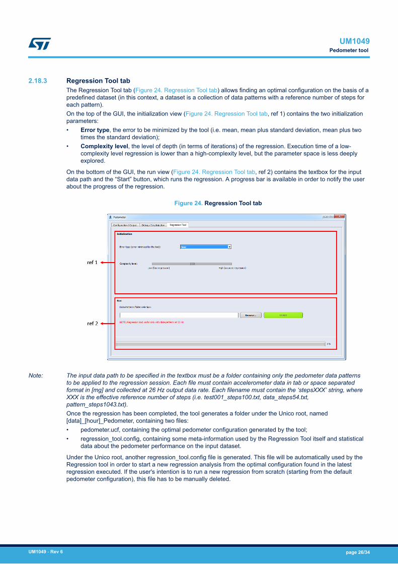
2.18.3 Regression Tool tabThe Regression Tool tab (Figure 24. Regression Tool tab) allows finding an optimal configuration on the basis of apredefined dataset (in this context, a dataset is a collection of data patterns with a reference number of steps foreach pattern).On the top of the GUI, the initialization view (Figure 24. Regression Tool tab, ref 1) contains the two initializationparameters:• Error type, the error to be minimized by the tool (i.e. mean, mean plus standard deviation, mean plus two

times the standard deviation);• Complexity level, the level of depth (in terms of iterations) of the regression. Execution time of a low-

complexity level regression is lower than a high-complexity level, but the parameter space is less deeplyexplored.

On the bottom of the GUI, the run view (Figure 24. Regression Tool tab, ref 2) contains the textbox for the inputdata path and the “Start” button, which runs the regression. A progress bar is available in order to notify the userabout the progress of the regression.

Figure 24. Regression Tool tab

Note: The input data path to be specified in the textbox must be a folder containing only the pedometer data patternsto be applied to the regression session. Each file must contain accelerometer data in tab or space separatedformat in [mg] and collected at 26 Hz output data rate. Each filename must contain the ‘stepsXXX’ string, whereXXX is the effective reference number of steps (i.e. test001_steps100.txt, data_steps54.txt,pattern_steps1043.txt).Once the regression has been completed, the tool generates a folder under the Unico root, named[data]_[hour]_Pedometer, containing two files:• pedometer.ucf, containing the optimal pedometer configuration generated by the tool;• regression_tool.config, containing some meta-information used by the Regression Tool itself and statistical

data about the pedometer performance on the input dataset.

Under the Unico root, another regression_tool.config file is generated. This file will be automatically used by theRegression tool in order to start a new regression analysis from the optimal configuration found in the latestregression executed. If the user's intention is to run a new regression from scratch (starting from the defaultpedometer configuration), this file has to be manually deleted.

UM1049Pedometer tool

UM1049 - Rev 6 page 26/34

3 Data acquisition quick start

This section describes the basic steps that must be performed to acquire the data from the demonstration board:1. Plug the demonstration board into the USB port.2. Start the Unico GUI.3. Select the STEVAL-MKI according to the device/demonstration board in use (Figure 1. Unico launcher).4. Go to “Options” or “Registers” tab and click on “Easy Configuration” (Figure 3. Options tab, ref 1;

Figure 4. Register setup tab, ref 3)5. Click on the “Start” (or “Stop”) button to activate (or stop) the sensor data collection.6. Use the buttons on the left (Figure 2. Unico main window, ref 3) to display the desired tool.7. To close the application, click on the button “Exit” or simply close the main window.

UM1049Data acquisition quick start

UM1049 - Rev 6 page 27/34

4 Port detection

In some cases, the Unico software cannot automatically detect the port where the board is connected. In thesecases, the user needs to check the correct port and select it manually on the Unico GUI.This section describes how to detect the port for each operating system.

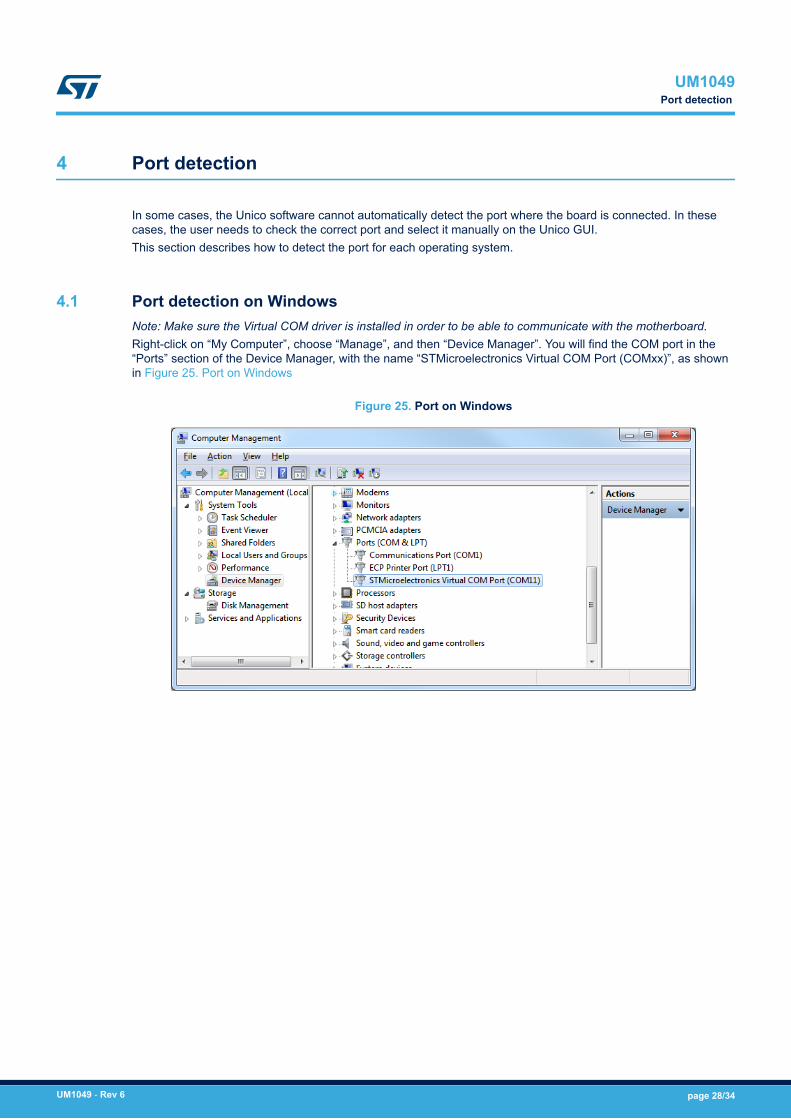
4.1 Port detection on WindowsNote: Make sure the Virtual COM driver is installed in order to be able to communicate with the motherboard.Right-click on “My Computer”, choose “Manage”, and then “Device Manager”. You will find the COM port in the“Ports” section of the Device Manager, with the name “STMicroelectronics Virtual COM Port (COMxx)”, as shownin Figure 25. Port on Windows

Figure 25. Port on Windows

UM1049Port detection

UM1049 - Rev 6 page 28/34

4.2 Port detection on Linux (Ubuntu)Just after connecting the board, open a terminal and type “dmesg”. The port will have a name similar to “ttyACM0”(or “ttyS0”), see details in Figure 26. Port on Linux.

Figure 26. Port on Linux

4.3 Port detection on Mac OSBefore connecting the board to your Mac, open a terminal and type:ls /dev/tty.*You will get a list of device files.Now, if you connect the board to your Mac and type the same command again, you will see a new filenamed /dev/tty.usbmodemXXX (the last three characters are numbers automatically assigned by the system).This means that the board is connected to the port usb.modemXXX.

UM1049Port detection on Linux (Ubuntu)

UM1049 - Rev 6 page 29/34

Revision history

Table 1. Document revision history

Date Revision Changes

02-Mar-2011 1 Initial release

06-Jun-2012 2

Added ‘Automatic COM Port Detection’ flag in Section 2: "Unico graphical user interface"

Updated Table 1: Device vs supported tabs including new supported devices

All figures have been updated

10-Sep-2013 3

Updated title of document

Updated Figure 1: "Unico Launcher"

Updated Table 1 with new supported devices and added “State machine” tab; removed obsoletedemonstration board (STEVAL-MKI063V1 based on the LSM303DLH)

Added Section 2.15: State machine tab

Minor textual updates

03-Nov-2014 4

Entire document revised according to release 4.0.0.0 of Unico• All figures updated• Linux and Mac OS subsections added to Section 1: "PC system requirements"• Removed irrelevant subsections and table from Section 2: "Unico graphical user interface"

and added Section 2.7: "Scatter plot tool"; Section 2.12: "State machine tool"; Section 2.16:"FFT tool" and Section 4: Port detection"

20-Oct-2016 5Added STEVAL-MKI109V3 to "Introduction"

Textual updates in Section 1.1: "Windows platforms" and Section 4.1: Port detection on Windows"

23-Jan-2019 6

Updated Introduction

Updated Section 2 Unico graphical user interface and Figure 1. Unico launcher

Updated Section 2.12 State machine tool

Updated Section 2.12.1 Configuration tab

Updated Section 2.12.2 Interrupt tab

Updated Section 2.12.3 Debug tab

Added Section 2.13 Machine Learning Core tool

Added Section 2.18 Pedometer tool

UM1049

UM1049 - Rev 6 page 30/34

Contents

1 PC system requirements. . . . . . . . . . . . . . . . . . . . . . . . . . . . . . . . . . . . . . . . . . . . . . . . . . . . . . . . . . .2

1.1 Windows platforms . . . . . . . . . . . . . . . . . . . . . . . . . . . . . . . . . . . . . . . . . . . . . . . . . . . . . . . . . . . . . 2

1.2 Linux platforms . . . . . . . . . . . . . . . . . . . . . . . . . . . . . . . . . . . . . . . . . . . . . . . . . . . . . . . . . . . . . . . . 2

1.3 Mac OS X platforms . . . . . . . . . . . . . . . . . . . . . . . . . . . . . . . . . . . . . . . . . . . . . . . . . . . . . . . . . . . . 2

2 Unico graphical user interface . . . . . . . . . . . . . . . . . . . . . . . . . . . . . . . . . . . . . . . . . . . . . . . . . . . . .3

2.1 Tools available . . . . . . . . . . . . . . . . . . . . . . . . . . . . . . . . . . . . . . . . . . . . . . . . . . . . . . . . . . . . . . . . . 4

2.2 Options tab. . . . . . . . . . . . . . . . . . . . . . . . . . . . . . . . . . . . . . . . . . . . . . . . . . . . . . . . . . . . . . . . . . . . 5

2.3 Register setup tab . . . . . . . . . . . . . . . . . . . . . . . . . . . . . . . . . . . . . . . . . . . . . . . . . . . . . . . . . . . . . . 6

2.4 Load/Save tab . . . . . . . . . . . . . . . . . . . . . . . . . . . . . . . . . . . . . . . . . . . . . . . . . . . . . . . . . . . . . . . . . 7

2.5 Bars tool . . . . . . . . . . . . . . . . . . . . . . . . . . . . . . . . . . . . . . . . . . . . . . . . . . . . . . . . . . . . . . . . . . . . . . 8

2.6 Plot tool . . . . . . . . . . . . . . . . . . . . . . . . . . . . . . . . . . . . . . . . . . . . . . . . . . . . . . . . . . . . . . . . . . . . . . 9

2.7 Scatter plot tool . . . . . . . . . . . . . . . . . . . . . . . . . . . . . . . . . . . . . . . . . . . . . . . . . . . . . . . . . . . . . . . 10

2.8 Data tool . . . . . . . . . . . . . . . . . . . . . . . . . . . . . . . . . . . . . . . . . . . . . . . . . . . . . . . . . . . . . . . . . . . . . 11

2.9 Interrupt tool. . . . . . . . . . . . . . . . . . . . . . . . . . . . . . . . . . . . . . . . . . . . . . . . . . . . . . . . . . . . . . . . . . 12

2.10 Compass tool. . . . . . . . . . . . . . . . . . . . . . . . . . . . . . . . . . . . . . . . . . . . . . . . . . . . . . . . . . . . . . . . . 13

2.11 FIFO tool . . . . . . . . . . . . . . . . . . . . . . . . . . . . . . . . . . . . . . . . . . . . . . . . . . . . . . . . . . . . . . . . . . . . 14

2.12 State machine tool . . . . . . . . . . . . . . . . . . . . . . . . . . . . . . . . . . . . . . . . . . . . . . . . . . . . . . . . . . . . 15

2.12.1 Configuration tab. . . . . . . . . . . . . . . . . . . . . . . . . . . . . . . . . . . . . . . . . . . . . . . . . . . . . . . . 15

2.12.2 Interrupt tab . . . . . . . . . . . . . . . . . . . . . . . . . . . . . . . . . . . . . . . . . . . . . . . . . . . . . . . . . . . 16

2.12.3 Debug tab . . . . . . . . . . . . . . . . . . . . . . . . . . . . . . . . . . . . . . . . . . . . . . . . . . . . . . . . . . . . . 17

2.13 Machine Learning Core tool. . . . . . . . . . . . . . . . . . . . . . . . . . . . . . . . . . . . . . . . . . . . . . . . . . . . . 18

2.13.1 Data Patterns tab . . . . . . . . . . . . . . . . . . . . . . . . . . . . . . . . . . . . . . . . . . . . . . . . . . . . . . . 18

2.13.2 Configuration tab. . . . . . . . . . . . . . . . . . . . . . . . . . . . . . . . . . . . . . . . . . . . . . . . . . . . . . . . 19

2.14 Click tool. . . . . . . . . . . . . . . . . . . . . . . . . . . . . . . . . . . . . . . . . . . . . . . . . . . . . . . . . . . . . . . . . . . . . 20

2.15 Inclinometer tool . . . . . . . . . . . . . . . . . . . . . . . . . . . . . . . . . . . . . . . . . . . . . . . . . . . . . . . . . . . . . . 21

2.16 6D tool . . . . . . . . . . . . . . . . . . . . . . . . . . . . . . . . . . . . . . . . . . . . . . . . . . . . . . . . . . . . . . . . . . . . . . 22

2.17 FFT tool . . . . . . . . . . . . . . . . . . . . . . . . . . . . . . . . . . . . . . . . . . . . . . . . . . . . . . . . . . . . . . . . . . . . . 23

2.18 Pedometer tool . . . . . . . . . . . . . . . . . . . . . . . . . . . . . . . . . . . . . . . . . . . . . . . . . . . . . . . . . . . . . . . 24

2.18.1 Configuration / Output tab . . . . . . . . . . . . . . . . . . . . . . . . . . . . . . . . . . . . . . . . . . . . . . . . . 24

UM1049Contents

UM1049 - Rev 6 page 31/34

2.18.2 Debug / Data Injection tab. . . . . . . . . . . . . . . . . . . . . . . . . . . . . . . . . . . . . . . . . . . . . . . . . 25

2.18.3 Regression Tool tab . . . . . . . . . . . . . . . . . . . . . . . . . . . . . . . . . . . . . . . . . . . . . . . . . . . . . 26

3 Data acquisition quick start . . . . . . . . . . . . . . . . . . . . . . . . . . . . . . . . . . . . . . . . . . . . . . . . . . . . . . .27

4 Port detection . . . . . . . . . . . . . . . . . . . . . . . . . . . . . . . . . . . . . . . . . . . . . . . . . . . . . . . . . . . . . . . . . . . .28

4.1 Port detection on Windows . . . . . . . . . . . . . . . . . . . . . . . . . . . . . . . . . . . . . . . . . . . . . . . . . . . . . 28

4.2 Port detection on Linux (Ubuntu). . . . . . . . . . . . . . . . . . . . . . . . . . . . . . . . . . . . . . . . . . . . . . . . . 29

4.3 Port detection on Mac OS . . . . . . . . . . . . . . . . . . . . . . . . . . . . . . . . . . . . . . . . . . . . . . . . . . . . . . 29

Revision history . . . . . . . . . . . . . . . . . . . . . . . . . . . . . . . . . . . . . . . . . . . . . . . . . . . . . . . . . . . . . . . . . . . . . . .30

UM1049Contents

UM1049 - Rev 6 page 32/34

List of figuresFigure 1. Unico launcher . . . . . . . . . . . . . . . . . . . . . . . . . . . . . . . . . . . . . . . . . . . . . . . . . . . . . . . . . . . . . . . . . . . . 3Figure 2. Unico main window . . . . . . . . . . . . . . . . . . . . . . . . . . . . . . . . . . . . . . . . . . . . . . . . . . . . . . . . . . . . . . . . . 4Figure 3. Options tab . . . . . . . . . . . . . . . . . . . . . . . . . . . . . . . . . . . . . . . . . . . . . . . . . . . . . . . . . . . . . . . . . . . . . . 5Figure 4. Register setup tab. . . . . . . . . . . . . . . . . . . . . . . . . . . . . . . . . . . . . . . . . . . . . . . . . . . . . . . . . . . . . . . . . . 6Figure 5. Load/Save tab . . . . . . . . . . . . . . . . . . . . . . . . . . . . . . . . . . . . . . . . . . . . . . . . . . . . . . . . . . . . . . . . . . . . 7Figure 6. Bars tool . . . . . . . . . . . . . . . . . . . . . . . . . . . . . . . . . . . . . . . . . . . . . . . . . . . . . . . . . . . . . . . . . . . . . . . . 8Figure 7. Plot tool . . . . . . . . . . . . . . . . . . . . . . . . . . . . . . . . . . . . . . . . . . . . . . . . . . . . . . . . . . . . . . . . . . . . . . . . . 9Figure 8. Scatter plot tool . . . . . . . . . . . . . . . . . . . . . . . . . . . . . . . . . . . . . . . . . . . . . . . . . . . . . . . . . . . . . . . . . . 10Figure 9. Data tool . . . . . . . . . . . . . . . . . . . . . . . . . . . . . . . . . . . . . . . . . . . . . . . . . . . . . . . . . . . . . . . . . . . . . . . 11Figure 10. Interrupt tool. . . . . . . . . . . . . . . . . . . . . . . . . . . . . . . . . . . . . . . . . . . . . . . . . . . . . . . . . . . . . . . . . . . . . 12Figure 11. Compass tool . . . . . . . . . . . . . . . . . . . . . . . . . . . . . . . . . . . . . . . . . . . . . . . . . . . . . . . . . . . . . . . . . . . . 13Figure 12. FIFO tool . . . . . . . . . . . . . . . . . . . . . . . . . . . . . . . . . . . . . . . . . . . . . . . . . . . . . . . . . . . . . . . . . . . . . . . 14Figure 13. Configuration tab . . . . . . . . . . . . . . . . . . . . . . . . . . . . . . . . . . . . . . . . . . . . . . . . . . . . . . . . . . . . . . . . . 15Figure 14. Interrupt tab . . . . . . . . . . . . . . . . . . . . . . . . . . . . . . . . . . . . . . . . . . . . . . . . . . . . . . . . . . . . . . . . . . . . . 16Figure 15. Debug tab . . . . . . . . . . . . . . . . . . . . . . . . . . . . . . . . . . . . . . . . . . . . . . . . . . . . . . . . . . . . . . . . . . . . . . 17Figure 16. MLC Data Patterns tab . . . . . . . . . . . . . . . . . . . . . . . . . . . . . . . . . . . . . . . . . . . . . . . . . . . . . . . . . . . . . 18Figure 17. MLC Configuration tab. . . . . . . . . . . . . . . . . . . . . . . . . . . . . . . . . . . . . . . . . . . . . . . . . . . . . . . . . . . . . . 19Figure 18. Click tool . . . . . . . . . . . . . . . . . . . . . . . . . . . . . . . . . . . . . . . . . . . . . . . . . . . . . . . . . . . . . . . . . . . . . . . 20Figure 19. Inclinometer tool . . . . . . . . . . . . . . . . . . . . . . . . . . . . . . . . . . . . . . . . . . . . . . . . . . . . . . . . . . . . . . . . . . 21Figure 20. 6D tool . . . . . . . . . . . . . . . . . . . . . . . . . . . . . . . . . . . . . . . . . . . . . . . . . . . . . . . . . . . . . . . . . . . . . . . . 22Figure 21. FFT tool. . . . . . . . . . . . . . . . . . . . . . . . . . . . . . . . . . . . . . . . . . . . . . . . . . . . . . . . . . . . . . . . . . . . . . . . 23Figure 22. Configuration / Output tab . . . . . . . . . . . . . . . . . . . . . . . . . . . . . . . . . . . . . . . . . . . . . . . . . . . . . . . . . . . 24Figure 23. Debug / Data Injection tab . . . . . . . . . . . . . . . . . . . . . . . . . . . . . . . . . . . . . . . . . . . . . . . . . . . . . . . . . . . 25Figure 24. Regression Tool tab . . . . . . . . . . . . . . . . . . . . . . . . . . . . . . . . . . . . . . . . . . . . . . . . . . . . . . . . . . . . . . . 26Figure 25. Port on Windows. . . . . . . . . . . . . . . . . . . . . . . . . . . . . . . . . . . . . . . . . . . . . . . . . . . . . . . . . . . . . . . . . . 28Figure 26. Port on Linux . . . . . . . . . . . . . . . . . . . . . . . . . . . . . . . . . . . . . . . . . . . . . . . . . . . . . . . . . . . . . . . . . . . . 29

UM1049List of figures

UM1049 - Rev 6 page 33/34

IMPORTANT NOTICE – PLEASE READ CAREFULLY

STMicroelectronics NV and its subsidiaries (“ST”) reserve the right to make changes, corrections, enhancements, modifications, and improvements to STproducts and/or to this document at any time without notice. Purchasers should obtain the latest relevant information on ST products before placing orders. STproducts are sold pursuant to ST’s terms and conditions of sale in place at the time of order acknowledgement.

Purchasers are solely responsible for the choice, selection, and use of ST products and ST assumes no liability for application assistance or the design ofPurchasers’ products.

No license, express or implied, to any intellectual property right is granted by ST herein.

Resale of ST products with provisions different from the information set forth herein shall void any warranty granted by ST for such product.

ST and the ST logo are trademarks of ST. All other product or service names are the property of their respective owners.

Information in this document supersedes and replaces information previously supplied in any prior versions of this document.

© 2019 STMicroelectronics – All rights reserved

UM1049

UM1049 - Rev 6 page 34/34