unep/ipcs - who
TRANSCRIPT

UNEP/IPCS
Training Module No. 3
CHEMICAL
RISK ASSESSMENT
HUMAN RISK ASSESSMENT,
ENVIRONMENTAL RISK ASSESSMENT
AND ECOLOGICAL RISK ASSESSMENT
1999
The views expressed in documents by named authors are
solely the responsibility of those authors.
Produced under the joint sponsorship of the United Nations Environment Programme,
the International Labour Organisation and the World Health Organization, and within the framework of the Inter-Organization Programme
for the Sound Management of Chemicals

The International Programme on Chemical Safety (IPCS), established in 1980, is a joint venture of the United Nations Environment Programme (UNEP), the International Labour Organisation (ILO), and the World Health Organization (WHO). The overall objectives of the IPCS are to establish the scientific basis for assessing the risk to human health and the environment from exposure to chemicals, through international peer-review processes, as a prerequisite for the promotion of chemical safety, and to provide technical assistance in strengthening national capacities for the sound management of chemicals.
The Inter-Organization Programme for the Sound Management of Chemicals (IOMC) was established in 1995 by UNEP, ILO, the Food and Agriculture Organization of the United Nations, WHO, the United Nations Industrial Develop- ment Organization, and the Organisation for Economic Co- operation and Development (Participating Organizations), following recommendations made by the 1992 United Nations Conference on Environment and Development to strengthen cooperation and increase coordination in the field of chemical safety. The purpose of the IOMC is to promote coordination of the policies and activities pursued by the Participating Organizations, jointly or separately, to achieve the sound management of chemicals in relation to human health and the environment.

ACKNOWLEDGEMENT
The International Programme on Chemical Safety (IPCS) is a joint venture of the United Nations Environment Programme (UNEP), the International Labour Organisation (ILO) and the World Health Organization (WHO). Amongst its many activities are training programmes on risk assessment and risk management of chemicals for which a series of Training Modules is being developed.
This Training Module on Risk Assessment was prepared by Dr J.H. Dufis and Dr M.V. Park, The Edinburgh Centre for Toxicology, Edinburgh, U.K. The technical development, field testing, editing and publication of the Module has been coordinated by UNEP Chemicals (IRPTC), Geneva, Switzerland, as UNEP' S contribution to the training activities being conducted by the IPCS. No language editing of the Module has been conducted by the IPCS Central Unit.
The draft Training Module was tested at a series of IPCS Training Courses on Toxic Chemicals, Environment and Health - Dhaka, Bangladesh, March 1997; Bandung, Indonesia, May 1997; Colombo, Sri Lanka, July 1997; Islamabad, Pakistan, October 1997; Mukono, Uganda, March 1 998; Harare, Zimbabwe, March 1998; Montevideo, Uruguay, November 1998; Buenos Aires, Argentina, November 1998 - with financial support from the Government of the Kingdom of the Netherlands, and at two workshops, namely: the National Workshop on Chemical Risk Assessment, Moscow (Golitsino), Russian Federation, October 1997; and the Subregional Workshop on Chemical Risk Assessment, Bratislava (Senec), Slovakia, November 1997. Funds were provided by the Government of the Russian Federation and the Government of Austria.
The IPCS gratefully acknowledges the work undertaken by the authors, Dr Duf is and Dr Park, and by UNEP, and thanks all who helped in the preparation and finalization of this book for their efforts. Financial support for the publication was provided by the Netherlands Ministry of Development and Cooperation under the auspices of the IPCS Project on National Training Activities for Developing Countries on Toxic Chemicals, Environment and Health.
iii

Contents
Page
Section A: Human Risk Assessment 1
Section B: Environmental Risk Assessment 107
Section C: Ecological Risk Assessment 177
IV

UNEPIIPCS Training Module No. 3
Section A
Human Risk Assessment


UNEPllPCS TRAINING MODULE SECTION A
Human Risk Assessment
TABLE OF CONTENTS
PAGE EDUCATIONAL OBJECTIVES ............................................................................. 4 1 Introduction ...................................................................................................... 4 2 Definitions ........................................................................................................ 5
2.1 Hazard ................................................................................................. 5
2.2 Exposure ............................................................................................. 5 2.3 Risk ..................................................................................................... 6
2.4 Dose-response and dose-effect relationships ..................................... 6 ........................................................................... 2.5 Risk characterisation 7
2.6 Risk assessment ................................................................................ 7 3 How does one carry out Risk Assessment? .................................................... 7
3.1 Introduction ........................................................................................ 7 3.1. l Hazard identification .......................................................... 8 3.1.2 Dose (concentration) - response (effect) relation .................. 8 3.1.3 Exposure assessment ....................................................... 8 3.1.4 Risk characterisation ............................................................. 8
3.2 Identification of the hazard .................................................................. 9
............................................................... 3.2.1 Nature of Hazards 10 3.2.1 . 1 Hazards to health .................................................. 10 3.2.1.2 Physico-chemical hazards ..................................... l l
3.2.2 Sources of hazard information ............................................ 12 3.2.3 Assessment of the hazard ................................................... 15
3.2.3.1 Toxicological hazards ............................................ 15 3.2.3.2 Physico-chemical hazards ..................................... 16
3.3 Determination of the dose (concentration) - response (effect) ............................................................................................. relation 17
................................. 3.3.1 Threshold and Non-Threshold Effects 18 3.3.2 Threshold Effects ............................................................. 19
3.3.2.1 Occupational Exposure ......................................... 19 3.3.2.2 Non-Occupational Exposure ................................. 20 3.3.2.3 Margins of Safety or of Exposure .......................... 24 3.3.2.4 Other Approaches ................................................ 24

3.3.2.5 Differences in approach between the occupational and the non-occupational situation .............................. 26
................................................................. 3.3.3 Benchmark Dose 27 3.3.4 Non-Threshold Effects ........................................................ 28
3.3.4.1 Quantitative extrapolation ...................................... 28 3.3.4.2 Ranking of potencies ............................................ 30 3.3.4.3 Modification of the highest "no effect" level ........... 30
3.4 Exposure assessment ....................................................................... 30
3.4.1 General aspects .................................................................. 30 3.4.1 . 1 Introduction ............................................................ 30 3.4.1.2 Types of exposure ................................................. 32 3.4.1.3 Modelling ........................................................... 33
3.4.2 Occupational Exposure ...................................................... 35 ............................................................ 3.4.2. l Introduction 35
............................................... 3.4.2.2 Inhalation exposure 36 3.4.2.3 Dermal exposure .............................................. 3 7 3.4.2.4 Measurement of exposure ...................................... 38
............................................................ 3.4.3 Consumer exposure 41 3.4.4 Indirect exposure via the environment ................................ 42
......................................................................... 3.5 Risk characterisation 42 ........ 3.5.1 General principles for assessing risk to human health 42
............................................ 3.5.2 Guidance or Guideline Values 44
3.5.3 Semi-quantitative assessment of risk from chemicals in the ............................................................................ workplace 45
4 Control of risk ................................................................................................. 46 .................................................... 4.1 Modification of process conditions 47
................................................ 4 .l . 1 Elimination and substitution 47
.......................................... 4.1.2 Containment and ventilation 4 7 ......... 4.1.2.1 Complete enclosure with exhaust ventilation 48
4.1.2.2 Partial enclosure with exhaust ventilation ............... 48 .............................. 4.1.2.3 Local exhaust ventilation (LEV) 48
..................................................................... 4.1.3 Open working -49 ........................................... 4.1.4 Personal protective equipment 4 9
................ 4.1.4.1 Respiratory protective equipment (RPE) 49
4.2 Fire and explosion .......................................................................... 50
4.3 Emergency planning ......................................................................... 50 5 Conclusion ...................................................................................................... 51
.................................................................................................. 6 Bibliography 5 2
7 Self Assessment Exercises ............................................................................ 54
ANNEX 1 . Animal toxicity testing of chemicals ................................................. 57 ................................................................................... ANNEX 2 . Risk Phrases 62
................................................................................ ANNEX 3 . . Safety Phrases 67
ANNEX 4 . Toxicological classification and labelling of dangerous substances 71 ANNEX 5 . Estimation of the tolerable intake of a chlorinated hydrocarbon
from toxicity data ............................................................................. 78
ANNEX 6 . Extrapolations between species of the effects of substances taken by the oral route ............................................................................ 80
ANNEX 7 . Modelling of airborne concentrations of volatile liquids in the ..................................................................................... workplace 8 3
.............. ANNEX 8 . Case study: contamination of room with metallic mercury 85
................................................................... ANNEX 9 . Exposure-route models 87 ..................................................................................... ANNEX 1 0 . Biomarkers 8 9
ANNEX 11 . An example on the development of guidance values ...................... 91

UNEPIIPCS TRAINING MODULE
SECTION A
Human Risk Assessment
EDUCATIONAL OBJECTIVES
You should know the difference in meaning of the terms "hazard" and "risk" and the
four stages of risk assessment. You should know the commonest routes by which
substances are absorbed into the body and be able to differentiate between: acute
and chronic effects, local and systemic effects, and reversible and irreversible
effects. You should be familiar with the problems in extrapolating the results of
studies of the harmful effects of substances from animals to humans and know what are the main sources of hazard information on commercially available substances. You should understand the difference between stochastic and deterministic (or non-
stochastic) effects and know how can one assess the relative toxicities of substances postulated to have no threshold level. You should be aware of how
exposure standards are set. You should know how parficulates are characterised and how they can cause harm. You should understand the principles of exposure
assessment and the use of biomarkers. You should know some of the common
approaches to minimising risk and how to progress from risk assessment to risk
management.
I INTRODUCTION
There has been a dramatic increase in the use of chemicals in recent years, many of
them new compounds and mixtures whose toxicological properties have not
previously been studied and which might prove to be harmful to humans. Over the
last fifty years several substances previously thought to be inert or harmless in
humans have been found to be carcinogenic (e.g. asbestos minerals) or toxic to the
reproductive process (e.g. thalidomide). A wide and increasing range of compounds
have been shown to be mutagenic or carcinogenic in animal studies.
Consequently, in spite of our limited knowledge of the hazards to humans
associated with many substances, most governments in the developed world, as
4

part of their function to protect their populations, have developed legislation aimed at
protecting both the working and the general population. This has usually required
the management of enterprises to eliminate or at least to minimise any risks
associated with their work both to their workers and to the general population.
In this section we shall be considering how one sets out to carry out a human risk
assessment with a particular emphasis on chemical substances in the workplace.
In general parlance, the words "hazard" and "risk" have become confused.
However, more correctly, they have two different meanings: "hazard" means
exclusively the qualitative description of harmful effects, whereas "risk" refers to a
quantitative measure of the probability for certain harmful effects to occur in a
group of people as the result of an exposure. The risk involved in a particular
process can often be reduced, usually at a cost, by appropriate engineering
measures, e.g. improved containment. What is considered an acceptable risk is a
decision that has to be left to society in general, to management, or to the individual,
as appropriate.
2 DEFINITIONS
Following are the definitions' of some terms commonly met with in risk assessment
2.1 Hazard
Set of inherent properties of a substance, mixture of substances or a process
involving substances that, under production, usage or disposal conditions,
make it capable of causing adverse effects to organisms or the environment,
depending on the degree of exposure; in other words it is a source of danger
2.2 Exposure
In this context it is defined as: the concentration, amount or intensity of a
particular physical or chemical agent or environmental agent that reaches the
target population, organism, organ, tissue or cell, usually expressed in
numerical terms of substance concentration, duration and frequency (for chemical agents and micro-organisms) or intensity (for physical agents such
IUPAC (1993) Glossary for chemists of terms used in toxicology, Pure & Appl. Chem. 65, 2003- 2122.
5

as radiation); the term can also be applied to the process by which a
substance becomes available for absorption by the target population,
organism, organ, tissue or cell, by any route.
2.3 Risk
Risk expresses the likelihood that the harm from a particular hazard is realised, and
is a function of hazard and exposure. More formally it can be defined as: the
possibility that a harmful event (death, injury or loss) arising from exposure to
a chemical or physical agent may occur under specific conditions; or
alternatively, the expected frequency of occurrence of a harmful event (death,
injury or loss) arising from exposure to a chemical or physical agent under
specific conditions.
2.4 Dose-res~onse and dose-effect relationshim
In Toxicology a distinction is made between the dose- (or concentration-) response
curve and the dose- (or concentration-) effect curve.
The dose-response curve can be defined as: the graph of the relation between
dose and the proportion of individuals responding with an all-or-none effect,
and is essentially the graph of the probability of an occurrence (or the proportion of a population exhibiting an effect) against dose. Typical examples of such all-or-none
effects are-mortality or the incidence of cancer.
In contrast, the dose-effect curve is the graph of the relation between dose and
the magnitude of the biological change produced, measured in appropriate
units. It applies to measurable changes giving a graded response to increasing
doses of a drug or xenobiotic. It represents the effect on an individual animal or
person, when biological variation is taken into account. Examples might be changes
in body weight, blood pressure or an enzyme level produced by increasing doses of
a drug, or increasing respiratory irritation resulting from exposure to increasing
concentrations of a toxic gas such as chlorine.

2.5 Risk characterisation
This stage, also referred to as risk estimation, is the quantitation of the risk following
consideration of the exposure and the dose-response (effect) relationship. It can be
defined as follows.
Assessment, with or without mathematical modelling, of the probability and
nature of effects of exposure to a substance based on quantification of dose-
effect and dose-response relationships for that substance and the
population(s) and environmental components likely to be exposed and on
assessment of the levels of potential exposure of people, organisms and
environment at risk.
2.6 Risk assessment
This process is a scientific attempt to identify and estimate the true risks, and is the resultant of the considerations of its components above: the hazard, dose-response
(effect) relationship, and risk characterisation. It can be defined as follows.
The identification and quantification of the risk resulting from a specific use or
occurrence of a chemical or physical agent, taking into account possible
harmful effects on individual people or society of using the chemical or
physical agent in the amount and manner proposed and all the possible routes
of exposure. Quantification ideally requires the establishment of dose-effect
and dose-response relationships in likely target individuals and populations.
If following a Risk Assessment the conclusion is that there is still an important risk inherent which cannot be reduced further, we pass into the area of Risk Management, where decisions on whether or not to proceed will involve a mixture of economic, societal and political factors.
3 HOW DOES ONE CARRY OUT RISK ASSESSMENT?
3.1 Introduction
There are normally four stages in this, as follows.
7
3.1 .l Hazard identification What are the substances of concern and what are their adverse effects?
3.1.2 Dose (concentration) - response (effect) relation What is the relationship between the dose and either the severity or the frequency of
the effect (dose-effect and dose-response relationships respectively)?
3.1.3 Exposure assessment What is the intensity, and the duration or frequency of exposure to an agent?
3.1.4 Risk characterisation How can one quantify the risk from the above data?
A risk assessment of the effect of chemical substances would normally examine the following potential toxic effects by each of the likely routes of exposure - oral (by
ingestion), dermal (by absorption through the skin) and inhaled in the breath. It would also examine the human populations affected.
Effects:' 8
e
8
e
8
e
e
e
Acute toxicity Irritation
Corrosiveness Sensitisation
Repeated dose toxicity Mutagenicity Carcinogenicity Toxicity for reproduction
By far the greatest part of information about these different effects has been obtained from studies on animals. In most cases where different routes of exposure are possible (oral, dermal, or by inhalation), the choice of route of administration
depends on the physical characteristics of the test substance and the form typifying exposure in humans. An explanation of these different effects and of the nature of the tests used to characterise them is given in Annex 1.

The human populations affected can be conveniently divided into three groups, with
some characteristics of each and expected exposure routes as follows:
0 Workers (exposed occupationally) - exposure assumed during working week - 8h day, 5 days per
week? - relatively healthy part of general population - exposure routes: normally inhalation and dermal only
Consumers (exposed to retail consumer products) - exposure intermittent - needs to be estimated - exposures may not be well controlled - exposure routes: oral, inhalation andlor dermal
Human population exposed indirectly via the environment - exposure 24h per day, 365 days in year - includes weak and unhealthy groups, e.g. children and elderly
people - exposure routes: oral, inhalation andlor dermal
3.2 Identification of the hazard
The first stage of any risk assessment is the identification of any substances or processes which might have an adverse effect on both involved workers and the
general public, and of those potentially exposed to them. Any process involving the handling of such substances may be hazardous as a result of their intake into the body, mainly by inhalation through the respiratory tract, or by dermal routes through the skin. Intake by injection or ingestion is not usually important as far as those occupationally exposed are concerned, as these routes can be easily avoided, but
ingestion can be a significant source of intake for members of the general public. Consideration should also be given to the possibility of accidental injection or ingestion. Their adverse effects may arise from the biological effects of their intake, from the presence of pathological micro-organisms, or, if radioactive, from internal radiation following ingestion or external radiation if handled or near-by. If
substances are explosive or flammable, there are obvious dangers associated with them.
Normally when carrying out a risk assessment of an enterprise one would divide its total work into its individual activities and assess each work activity separately. Consideration would also have to be given to activities such as maintenance, the
removal- of hazardous wastes, and to staff who may only occasionally be in the
working area.
With established commercial substances there is usually an extensive database of both their physico-chemical and their toxicological properties, the latter arising from studies on animals and case reports on humans, and often from epidemiological studies. This information has been used to classify many chemical substances and
preparations according to the type and potency of the hazard. This classification is an important source of hazard information, and is found on product labels and
datasheets (see later).
With new or unusual substances or processes this hazard information may not be so readily available, and their potential harmfulness may have to be assessed by a
variety of methods, including surveys of the scientific literature, observation and experimental work, and deductive work based on physico-chemical properties and
structure-activity relationships.
3.2.1 Nature of Hazards
3.2.1.1 Hazards to health
Hazards to health of substances can be conveniently divided into the following
groups:
0 acute and chronic effects e local and systemic effects
reversible and irreversible effects.
Acute and chronic effects. An acute effect is one that manifests itself after a single
exposure (or after a very few repeated exposures), such as the asphyxiation, unconsciousness or death produced by overexposure to solvent vapours. In contrast, a chronic effect will only be observed following repeated exposure to a substance over a long period of time. An example of this is silicosis following exposure to crystalline silica dust over a long period.

Local and systemic effects. A local effect occurs at the point of contact of the substance and the body, for example the effect of a corrosive substance splashed on the skin. In systemic effects, however, the action of the substance takes place at a point remote from where it entered the body. An example of this would be the
damage to the kidney by cadmium ions following their ingestion.
Reversible and irreversible effects. In reversible effects, the tissue of the person recovers and returns to normal when the exposure ceases. Examples would be skin
irritation and anaesthesia. Where the effect is irreversible, as in cancer, this recovery does not take place.
In many cases the situation is more accurately described by using these terms in combination. For example, skin irritation is an acute, local, reversible effect,
whereas liver cancer is chronic, systemic and irreversible.
With some toxic effects, it can be difficult to decide which of these categories apply, for example where there is a preliminary sensitisation following chronic exposure
which results in a later acute effect, or where a compound has an adverse effect on reproduction.
Finally, much of the evidence for the harmful effects of substances is based on animal studies in which rats and mice have been exposed to very high doses, very
often given by the oral route. In contrast, occupational exposure is much more likely to be by the respiratory tract or by absorption through the skin. There are therefore a number of imponderables in extrapolating data based on studies of the ingestion of high doses by rodents to the human situation, where the doses are often much lower and absorbed by a different route. This is of particular relevance to potential carcinogens, which may show a dose-dependent metabolism - the nature of the metabolites and their proportions being dependent on the magnitude of the dose - and consequently such studies may give rise to results which are difficult to
interpret.
3.2. l .2 Physico-chemical hazards
The main hazards in this group are fire and explosion.
The flammability of a substance depends on how reactive it is with oxygen, its physical form and its volatility.

Fire involving flammable vapours can only occur when they are mixed with air or
oxygen within certain proportions - lower and upper explosive limits (flammable limits). For most flammable solvents the lower explosive limit is in the range 1 - 5%
of solvent in air. This lower limit is usually considerably greater than the
recommended exposure limit in the working environment.
Many vapours are heavier than air and may spread unnoticed some distance from their source, giving rise to the danger of flashback if ignited. It is therefore good
working practice to keep the atmospheric concentration within any plant below a
quarter of the lower explosive limit.
It should be noted that the energy for the ignition of certain flammable vapours, such
as those of carbon disulfide and some ethers and aldehydes, may come from
unexpected sources such as hot plates, ovens and heating mantles. Sparks caused
by static electricity or electric switchgear have also been known to ignite flammable
vapours, gases and dusts. This underlines the need to avoid flammable
concentrations.
Only a small number of substances can explode as a result of shock, friction, fire or
other sources of ignition, and for commercially available substances this property would be indicated on the label. However, a number of flammable substances can
burn with explosive force given suitable conditions.
3.2.2 Sources of hazard information
It is important that hazard information used in an assessment is reliable and current.
For commercially available substances, the principal sources are from
e Chemical Safety Data Sheets supplied by the manufacturer or supplier e Product labels (see following)
* Information from governmental and trade associations * Other information may be obtained from the established technical literature.

Normally when dealing with well-known substances produced by reputable
manufacturers, the data supplied by them should be sufficient to assess the hazard
associated with the use of the substance.
In many countries manufacturers, suppliers and importers of chemical substances
are responsible for classifying and labelling the substances they supply and for
supplying further information about them in the form of "Chemical Safety Data
Sheets" (the types of information covered by such sheets are shown in Table 1).
This is to ensure that the toxicological and physico-chemical properties that make a
substance dangerous have been both identified and publicised to the user.
In one system of classification' on the basis of toxicological properties the labelling
comprises hazard symbols along with standard "risk" phrases, to identify the
hazards associated with the substance, and "safety" phrases, giving advice on their
handling. Each of these standard phrases is associated with a unique "risk or
"safety" number, e.g. R23 or S12. The label should contain the following
information:
Name or names of the substances which will appear on the label 0 The name, address and telephone number of the person responsible for placing
the substance or preparation on the market
The symbols and indication of danger Phrases indicating particular hazards (R-phrases)
Phrases indicating safety advice (S-phrases)
For substances, the EEC number.
A list of Risk phrases is given in Annex 2. and of Safety Phrases in Annex 3.
The label should also take into account all potential hazards likely to arise in normal
handling and use of a dangerous substance in the form in which it is supplied - although not necessarily in any different form in which it may ultimately be used, e.g.
diluted.
2 European Union Council Directive 671548lEEC.
13

The information describing all adverse biological effects of a particular substance on
humans allow it to be allocated to one of the following categories:
Very toxic (by ingestion, inhalation or skin contact)
Toxic (by ingestion, inhalation or skin contact)
Harmful (by ingestion, inhalation or skin contact)
Corrosive (to skin)
Irritant (to respiratory tract, skin or eyes)
The category and nature of the adverse biological effect is indicated by the hazard
symbol and by the Risk phrase(s) or number(s).
Classification on the basis of physico-chemical properties is concerned with
flammability, and explosive and oxidising properties. The different categories are:
Extremely flammable
Highly flammable
Flammable
Explosive
Oxidising
Oxidising substances may render other substances flammable (e.g. certain organic
and inorganic peroxides) or explosive.
There are separate hazard symbols for highly or extremely flammable, explosive
and oxidising substances.
Examples of hazard symbols for the different categories of danger are given in Table
2. The basis of the allocation of substances to these toxicological categories in this
system is discussed more fully in Annex 4.
For recently introduced commercial substances, similar information will be available
as a result of the requirement in many countries for notification of a "base set"
dossier of toxicological and other data (See Section B, "Environmental Risk
Assessment", Annex1 ).

However, it should be noted that for many traditional substances (i.e. other than
those relatively recently introduced), the available toxicological data may be inadequate scientifically in comparison with the "base set" dossier referred to above
and intelligent deductions may be the only substitute.
Where a completely new substance of unknown toxicology is used or produced, such as a newly synthesised compound in a research laboratory, it should be
treated as a high hazard unless there is good reason to think otherwise.
3.2.3 Assessment of the hazard
3.2.3.1 Toxicoloaical hazards
Substances that are toxicological hazards can be divided into four categories: e Special g High e Medium
e LOW
Table 3 shows one approach to the allocation of substances to these categories.
Where a mixture of substances is assessed, the overall hazard category should normally be that of the most hazardous component.
A substance of unknown toxicity should be considered as a high hazard unless there is good reason to think otherwise.
Special hazard
Substances in this category, including carcinogens, mutagens, and compounds possessing reproductive toxicity, are considered so dangerous that they must be assessed on an individual basis.
High hazard
These are substances labelled as "very toxic", "toxic", "corrosive" or which are skin sensitisers.

Medium hazard
Substances considered to be medium inhalation or ingestion hazards are labelled "harmful", and those of medium harm to the skin are labelled, "harmful" or "irritant".
Low hazard
These are substances that do not qualify for inclusion in any of the other hazard
categories.
3.2.3.2 Physico-chemical hazards
The main physico-chemical hazards are flammability and explosiveloxidising ability.
The emission of ionising radiation would also come under this heading, but this is a
less common hazard with the majority of commercial materials. In most countries it is covered by different legislation and is normally considered separately.
Flammability
This hazard is mainly associated with physical safety, although in some cases where
a toxic substance is produced by combustion or from the breakdown of materials used to extinguish a fire, a toxic hazard may result. For example, chloroform, a non-
flammable liquid, under certain fire conditions could give rise to the toxic gases phosgene (COCI,) and hydrogen chloride, and certain polymers used in furnishings may give rise to hydrogen cyanide on combustion.
Normally, for a liquid, flammability bears an inverse relationship to flash point: low flash point liquids tend to be associated with a very high hazard, whereas if the flash
point is high, it usually suggests a low hazard.
In many countries extremely and highly inflammable liquids are usually labelled with the danger symbol andlor letter, whereas flammable substances may only be indicated as such by a written inscription.
Some gases and solids are also combustible, but there are no standard criteria by which the flammability may be judged, compared with the flash point for liquids.
Explosive and oxidising ability
If the label indicates that the substance is explosive or oxidising, expert advice
should be sought regarding the particular precautions appropriate. If in doubt, reference should be made to the supplier.

3.3 Determination of the dose (concentration) - response (effect) relation
Having identified the hazard, it is now necessary to quantify it, i.e. to determine at
what concentration an adverse or toxic effect would be found. This is relatively easy for physical effects such as fire or explosion, but is much more difficult to determine for toxicological effects, particularly in the human, where for obvious reasons data are more limited. It is also necessary to bear in mind the effects of the length and frequency of exposure - is it continuous or only intermittent?
A variety of approaches have been used to derive this relationship. These include:
0 human observation, including case reports, epidemiological studies, and, in
some cases, direct human studies 0 animal toxicological studies o assessment of structure-activity relationships.
One approach to this problem is to carry out an epidemiological study. This has the
advantage of using medical findings in exposed persons to establish a dose - effect relationship without needing to know the mechanism of action, and it avoids the problems of extrapolating the results of animal studies to humans. However, all epidemiological studies are retrospective, and the occurrence of a cancer may occur several decades after the exposure. Also, the estimate of the level of exposure in such retrospective studies may be unsatisfactory, and in a practical context people are usually exposed to mixtures of substances rather than a pure one, introducing possible confounders. Finally, the size of the cohort studied may have to be a very
large one to identify, for example, a weak carcinogen.
For these reasons, a toxicological approach involving animal experimentation is usually essential. This has a number of obvious advantages, but it possesses the
major uncertainty of extrapolating the results from one species to another. These species differences can be quite considerable even between quite closely related species: e.g. dietary doses of the fungal toxin aflatoxin B, as high as 10 000 ppb failed to produce liver cancer in mice, whereas in the rat 15 ppb produced a significant increase. Presumably in many cases these differences arise from differences, quantitative or qualitative, in metabolism. Furthermore, decisions have to be made in planning the programme as to whether studies should be aimed at acute (short term), sub-chronic (medium term) or chronic (long-term) exposures, and

the route of the exposure. The advantages and disadvantages of data from animal
studies are summarised in Table 4.
There are particular uncertainties in studies of developmental or reproductive toxicity, immunotoxicity, or carcinogenicity. It may take as long as two years to obtain results in a study of a potential carcinogen, and in order to obtain statistically significant results in such studies with the minimum number of animals they may have to be exposed to high doses throughout their lifetimes, doses far in excess of the human exposure. In extrapolating to the results expected from low dose
exposure a linear relationship with a zero threshold is usually assumed: this may well not be the case. Lastly, the carcinogenic potential of a substance is likely to be related to its mode of exposure: injection of a substance may produce results different from those obtained from exposures by other more natural routes, such as
ingestion, intake through the respiratory tract or through the skin.
Structure-activity relationships (SAR) are estimation methods developed and used in order to predict certain effects or properties of chemical substances based on their
structures. As far as risk assessment for human health is concerned, it is a technique which is still very imperfect and in the developmental stage. As an approach, it is particularly useful for new substances where data from human or animal substances is limited and which are structurally related to other substances
of known toxicological properties. However, by its very nature, the approach can only be used for discrete organic substances and not for substances of unknown or variable composition, complex reaction mixtures, or biological materials.
3.3.1 Threshold and Non-Threshold Effects
The effects of a chemical on an organism can be divided into two types: those
considered to have to reach a threshold level before any adverse effects occur, and those postulated to have an adverse effect at any level, i.e. there is no harmless
dose.
Compounds possessing a threshold level are thought to be harmless at sufficiently low concentrations, i.e. they can be satisfactorily metabolised andlor excreted. However, in any one individual at higher doses above the threshold level increasingly severe effects are noted with increasing dose (Fig. 1).

Some harmful effects on individuals, such as cancers induced by radiation or
genotoxic chemicals, appear to act through a mechanism where a threshold cannot
be identified, and hence are assumed to have no threshold dose below which the
effect will not appear. In these cases it is the probability of occurrence of the effect
which depends on the absorbed dose, and hence they are referred to as stochastic
effects.
3.3.2 Threshold Effects
In assessing an acceptable level of a particular substance, the procedure usually
follows moving from an experimental database of animal or (preferably) human data
(e.g. from epidemiological studies) giving a No Observed Adverse Effect Level (NOAEL) or a Lowest Observed Adverse Effect Level (LOAEL) to deriving an
occupational exposure limit at a lower exposure value, to allow for the uncertainties
in the data. Comparison of this exposure limit with a measured or estimated
exposure level is then used to judge whether the situation is satisfactory or whether
risk management measures are required. Although these occupational limits
generally do not involve the determination of any specific "uncertainty factor" (in
contrast to non-occupational approaches), in practice the ratio of the NOAEL or
LOAEL to the limit appears to be in the range 1-10 for most substances where the
database is from animal studies, and of 1-2 when from human studies3.
One of the earliest moves towards an assessment of quantitative criteria with which
to judge the acceptability of measured exposure levels was the development of
Threshold Limit Values (TLV) in the 1940's by the American Conference of
Governmental Industrial Hygienists (ACGIH). The TLV is defined as the
concentration in air to which it is believed that most workers can be exposed daily
without an adverse effect (i.e. effectively the threshold between safe and dangerous
concentrations). The values were established (and are revised annually) by the
ACGIH and are time weighted concentrations for a 7 or 8 hour workday and a 40 hour workweek. These TLV's are based solely on health considerations and have
the status of recommended limits - they are not legally binding unless adopted by a regulatory agency.
Fairhurst, S. (1995) The uncertainty factor in the setting of occupational exposure standards. Annals of Occupational Hygiene, 39, 375-385.

This concept has developed steadily, and is now present in the legislation of most
developed countries. In the United States there is the National Institute for Occupational
Safety and Health (NIOSH)lOccupational Safety and Health Administration (OSHA) system of Permissible Exposure Limits (PEL) originally based on the ACGlH TLV values. OSHA is responsible for promulgating and enforcing these limits. In Germany there are Maximale Arbeitsplatzkonzentrationen (MAK, Maximum Concentration Values in the Workplace) and Technische Richtkonzentrationen (TRK, Technical
Exposure Limits), and in the Netherlands Nationale MAC-lijst (Maximale Aanvaarde Concentratie). The United Kingdom has a system of Occupational Exposure Standards (OES) and Maximum Exposure Limits (MEL), and the European Union is developing a system of Occupational Exposure Limits (OEL) which will apply to the
whole Union.
3.3.2.2 Non-Occupational Exposure
More structured schemes have been developed in deriving limits in non- occupational situations, most involving the application of uncertainty factors to the
lowest appropriate NOAEL to derive a human Tolerable Daily Intake (TDI), defined
as an estimate of the daily intake of a substance over a lifetime that is considered to be without appreciable health risk. Its units are commonly expressed in mg person-' day-' and assume a body weight of 60 kg. It is equivalent to the Acceptable Daily Intake (ADI), normally used of food additives, whose units,
however, are expressed on a body mass basis (usually mg kg-' day-'). Terms
analogous to the TDI, other than the ADI, are the Reference Dose (RfD) or the Reference Concentration (RfC).
The US Environmental Protection Agency Approach
After consideration of all available toxicological studies with a substance, the lowest typical NOAEL is chosen. Human studies are given the first priority, with animal toxicity studies ideally serving to complement them. However, most analyses are
based on non-human mammalian studies.
It is also assumed that any toxic effect is normally not dependent on the exposure route.
Where possible toxicokinetic studies of the substance are also taken into account,
and this could have a bearing on the selection of the critical data set used to

estimate the NOAEL. For example, the selection of an appropriate animal NOAEL might be based on similarities between the human and animal toxicokinetics.
Where it is not possible to decide which species has characteristics most relevant to
the human, the results from the animal species most sensitive to the substance are selected.
The NOAEL chosen is then used to determine a Reference Dose (RfD) by the use of Uncertainty Factors (UF), reflecting the overall confidence in the various data sets. In some cases Modifying Factors (MF), based on scientific judgement are
used.
The Uncertainty Factor (UF) is determined in the following way.
e If extrapolating from data from studies of healthy humans exposed over
prolonged periods, a factor of 10 is used. This factor is intended to take into
account variations in individual sensitivities in the human population.
e If the data has to be taken from long-term studies of animals because of a lack of
human data, a further factor of 10 is used. This is to account for possible inter-
species variation.
e If the data used is taken from only short-term studies of animals, a still further
factor of 10 is used. This is to account for the uncertainty in extrapolating from a less than chronic NOAEL to a chronic NOAEL.
Finally, if the RfD has to be derived from a LOAEL rather than a NOAEL, a further factor of 10 is used to account for the uncertainty in extrapolating from a LOAEL to a NOAEL
The Modifying Factor (MF) is greater than zero and can range up to 10. It depends on the professional assessment of the scientific uncertainties of the study and of the database not considered previously, e.g. the completeness of the overall database and the number of species tested. The default value is 1.
Hence the relationship between the NOAEL and the RfD is:

NOAEL = RfD X UF X MF
RfD = NOAEL UF X MF
According to the EPA, "...the RfD, which is indicated in mglkg bwlday, is an estimate (with uncertainty spanning perhaps an order of magnitude) of a daily exposure of a human population (including sensitive sub-groups) that is likely to be without an
appreciable risk of deleterious effects during a life-time". However, the EPA also
states that not all doses below the RfD are acceptable, but that all doses in excess of the RfD are unacceptable or will result in adverse effects.
Renwick Approach
Another approach to this problem is that of Renwick48 5. In Renwick's procedure, the
potential for modification of the two factors of 10 in the EPA scheme accounting for variation in the human population and inter-species variation is proposed. These
default values can be modified according to the extent of delivery of the substance to the site of toxicity (toxicokinetics) and the activity or potency of the substance at the site of toxicity (toxicodynamics). There is evidence that there is a greater
potential for differences in the kinetics than in the dynamics between humans and common laboratory animals, so that an unequal split was proposed into default
values of 2.5 (i.e. 1 O'.~) for dynamics and 4 for kinetics. For inter-individual differences between humans, the World Health Organization (WHO) through the
lnternational Programme on Chemical Safety (IPCS)G, in a review of Renwick's approach, recommended that at least in the interim an even split was more appropriate: 3.2 (1 oO.~) for kinetics, and 3.2 for dynamics.
Under the heading of toxicokinetics would be included data describing factors such as:
e rate and extent of absorption of the substance (bioavailability);
e peak plasma concentration (C,,) and area under the plasma concentration-
time curve (AUC) of the substance;
Renwick, A.G. (1991) Safety factors and establishment of acceptable daily intakes. Food Additives and Contaminants, 8, 135-1 50. Renwick, A.G. (1 993) Data-derived safety factors for the evaluation of food additives and environmental contaminants. Food Additives and Contaminants, 10, 275-305. World Health Organization (1 994) Assessing Health Risks of Chemicals: Derivation of Guidance Values for Health-based Exposure Limits. International Programme on Chemical Safety Environmental Health Criteria 170. Geneva: WHO.

e pattern of distribution in the body;
rate and pathway of any bioactivation;
rate, route and extent of elimination.
It is important to define which description of plasma concentration of the substance,
the peak plasma concentration (C,,,) or the area under the plasma concentration-
time curve (AUC), is relevant: in some cases the relevant parameter is C,,, rather
than AUC (e.g. the teratogenicity of valproic acid'), whereas in others it may be the
AUC.
The toxicodynamic factors of importance would include:
identification of the toxic entity (parent compound or a metabolite);
the presence and activity of protective and repair mechanisms; e in vitro sensitivity of the target tissue.
To modify the default inter-species values, information about these various
toxicokinetic and toxicodynamic factors would need to be available for the test
species and the human. Similar modification of the ten-fold factor for inter-individual
variability would require access to toxicokinetic and toxicodynamic data on a wide
and representative sample of the exposed human population. For the derivation of
limits for the whole population, which includes vulnerable groups such as the very
young, the sick, and the elderly, these factors are likely to be more stringent than
those applicable to the occupational situation, composed of a less vulnerable group
exposed under more controlled and monitored situations.
A procedure proposed by WHO for extrapolating from a toxicity data base to a
tolerable intake based on the Renwick procedure is shown in Fig. 2 8.
A simplified example of this type of extrapolation is discussed in Annex 5.
Nau, H. (1986) Species differences in pharmacokinetics and drug teratogenesis. Environ. Health Perspect., 70, 11 3-129; cited in World Health Organization ( l 994) Assessing Health Risks of Chemicals: Derivation of Guidance Values for Healfh-based Exposure Limits. lnternational Programme on Chemical Safety Environmental Health Criteria 170, p. 30. Geneva: WHO.
8 World Health Organization (1994) Assessing Health Risks of Chemicals: Derivation of Guidance Values for Health-based Exposure Limits. lnternational Programme on Chemical Safety Environmental Health Criteria 170, p. 33. Geneva: WHO.
23

3.3.2.3 Margins of Safety or of Exposure
A number of countries have abandoned the concept of Uncertainty Factors and
have substituted a different one, that of the margin of safety (MOS) or margin of exposure (MOE). In this procedure the ratio of the NOAEL determined in animals
and expressed in mg kg-1 day-1 is compared with the level to which a human may
be exposed:
MOS or MOE = NOA EL l mg kg-'day-'
Exposure l mg kg-'day-' '
For example, assuming the predominant exposure of the human population to a
substance is from its presence in drinking water at a concentration of 1 ppm, for a
60-kg woman consuming on average 2 L of water per day, then:
1 mg L-' X 2 L day-' Exposure =
60 kg
If the NOAEL for neurotoxicity is 100 mg kg-1 day-1, the margin of safety (MOS) will
be 10010.03, i.e. 3333, a reassuringly large value. However, should this value be much lower, it would indicate an inadequate MOS over the NOAEL - MOS values
below 100 have been interpreted by regulatory bodies as indicating a need for a more comprehensive evaluation. Note that this procedure does not take into
account differences in susceptibility between humans and animals nor within animals or humans, hence the relatively large magnitude of an MOS indicating
acceptable levels.
3.3.2.4 Other Approaches
ECETOC Approach
A procedure proposed by the European Centre for Ecotoxicology and Toxicology of Chemicals (ECETOC)g, a body set up by a number of major chemical companies in
1978 as a scientific non-commercial body, claims to include the best elements of
those procedures currently available. It aims to provide a method of deriving the
-
9 European Centre for Ecotoxicology and Toxicology of Chemicals (1 995) Assessment Factors in Human Health Risk Assessment (Technical Report No. 68). Brussels: ECETOC.

best scientific estimate of a human no adverse effect level, referred to as the
Predicted No Adverse Effect Level (PNAEL), takes into account the route and
duration of exposure and can be applied to both occupational and non-occupational
situations.
The initial stage is to decide which PNAEL's are required. This will involve
assessment of:
the nature of the exposed population (occupational, consumer, general public)
pattern and route of exposure (oral, inhalation, dermal);
acute or chronic exposure
single or occasional (acute) exposures - long-term repeated exposures
long-term continuous exposures
From this assessment it should be possible to determine the type(s) of human
PNAEL required. This will depend on the extent, duration and route of exposure.
Where a substance induces several effects, it is important to distinguish the less
severe (e.g. inflammation) from very severe (e.g. necrosis), and the reversible (e.g.
adaptive organ hypertrophy) from the irreversible (e.g. teratogenic effects).
From these properties of a substance, a critical effect for the human PNAEL is
chosen. This NOAEL may not necessarily be the lowest value, but it should be the
most appropriate and relevant to the situation.
Procedures are proposed for extrapolating from sub-chronic to chronic exposures,
from LOAEL to NOAEL, and from route to route; also for inter- and intra-species
extrapolation. Where appropriate recommended factor default values can be used
and a human PNAEL obtained by dividing the NOAEL(s) or LOAEL(s) by the
product of these factors (the overall "adjustment factor"). (A further discussion of the
procedures suggested in the ECETOC document for extrapolation between species
of the effects of substances taken by the oral route is given in Annex 6.)
The next stage is to allocate a degree of confidence or scientific uncertainty to the
PNAEL's derived above by assessing them as being associated with a high, medium
or low degree of confidence based on certain criteria. The PNAEL's are then

divided by the appropriate factors: 1 for a high degree of confidence; typically the range 1-2 for a medium degree of confidence; and a larger uncertainty factor for a
low degree of confidence.
This approach is summarised in Table 5, and an example of a Risk Assessment Worksheet using the ECETOC Procedure is given in Table 6.
3.3.2.5 Differences in approach between the occupational and the
non-occupational situation
There are a number of differences between occupational and non-occupational
situations that should be borne in mind. These include the following.
The PNAEL's required in an occupational situation may well differ from the
non-occupational case. Occupational exposure is often by inhalation, thus calling for a PNAEL for repeated exposure by that route, whereas exposure by the oral route, less likely in the workplace, is very likely in a non-occupational situation, requiring a different PNAEL.
The critical effects may be different because of these different routes of
exposure. For example, in many occupational situations the critical effect might be respiratory irritation. This effect is not likely to be relevant to a more likely lifetime oral exposure in the case of the general public.
A smaller adjustment factor may be appropriate in an occupational
situation when considering short-term repeated exposures. In the occupational context the exposure will follow a different pattern and be of shorter duration than a continuous lifelong non-occupational exposure.
A lower adjustment factor for inter-species extrapolation is often
appropriate when limits are obtained from inhalation studies than from
studies by the oral route. This is particularly applicable to the occupational situation, where exposure is more commonly by inhalation, and is discussed further in Annex 6.
0 The workplace population is less heterogeneous and in reasonable health
compared with the general population. The latter group includes a number of

people who might be particularly sensitive to the effects of a substance, e.g. the
very young, the chronically sick, and the elderly.
3.3.3 Benchmark Dose
The NOAEL approach has been criticised as having limitations in the following
respects.
e The NOAEL must by definition be one of the experimental doses tested - the
NOAEL is usually determined by setting it as the next lower dose below the
LOAEL.
e Once the NOAEL has been identified, the information contained in the remaining
data is ignored.
e The smaller the number of tests on experimental animals carried out, the larger
the apparent NOAEL is likely to be, thus rewarding the uncertainty associated
with less adequate test procedures. (The NOAEL represents a statistical "no
adverse effect" level.)
In the NOAEL approach, the "adverse effect" is not defined and hence the NOAEL will depend on the particular experimental design used.
To counter these objections an alternative approach has been proposed in which all the experimental data is used to fit one or more dose-response curves. These are then used to estimate a benchmark dose, defined as the statistical lower bound on a dose corresponding to a specified level of riskfo.
This procedure is illustrated in Fig. 3.11 A dose-response curve is modelled and fitted to the experimental data. The upper confidence limit on the estimated curve is obtained. The dose-response curve is used to estimate the dose that produces a low level of risk in the experimental dose range, e.g. the ED,,, the effective dose
corresponding to an excess risk of 10%. (There are often problems in estimating with adequate precision an excess risk of less than 10% above the background
l0 Allen, B C, Kavlock, R J, Kimmel, C A & Faustman, E M (1994) Dose-response assessment for developmental toxicity: II. Comparison of generic Benchmark Dose estimates with no observed adverse effect levels. Fundam. Appl. Toxicol., 23, 487-495.
l1 Kimmel, C A & Gaylor, D W (1988) Issues in qualitative and quantitative risk analysis for developmental toxicology. Risk Analysis, 8, 15-20.
27

level). From the upper confidence limit on that curve a lower confidence limit on the dose that produces a 10% risk (the LED,,) can be obtained.
If F represents a safety factor (e.g. loo), at a dose of LED,,/F the true unknown risk in the low dose region is expected to be less than O.I/F - as long as the dose-
response curve is curving upwards as in this example. This linear assumption will give conservative results from a safety standpoint.
This procedure has been applied to the study of several non-cancer areas of
toxicology, including developmental and reproductive toxicity, and has been found to give results similar to those from statistically derived NOAEL. Its advantage is that it makes much greater use of the information available, rather than simply the lowest
dose level at which effects are observed, and it also takes account of the
experimental variability of the data in the confidence limit.
3.3.4 Non-Threshold Effects
Examples of processes postulated as having no "threshold" are the effects of genotoxic carcinogens and of germ cell mutagens. There is not, however, any
general agreement on the appropriate methodology for dealing with these non-
threshold effects. Some of the approaches applied have been:
0 quantitative extrapolation by mathematical modelling of the dose-response
curve to estimate the risk at likely human intakes or exposures;
0 relative ranking of potencies as determined experimentally;
0 modification of the highest "no effect" level by dividing by an arbitrary
"uncertainty factor".
3.3.4.1 Quantitative extra~olation
The method used here is to obtain data on, e.g., tumour incidence at sufficiently high dose levels for the results to be statistically significant with the numbers of subjects or animals used, and to use an appropriate mathematical function to predict the incidence at very much lower dose levels. These functions range from simple proportionality at doses below that showing a significant effect, to much more complex models. There is obviously considerable uncertainty as regards the validity

of these models - quantitative extrapolations over several orders of magnitude may
be required.
This approach has been used by the lnternational Commission on Radiological
Protection (ICRP) in assessing the probability of a person dying from ionising
radiation-induced cancer. Because of the low probability of cancer induction at low
doses of radiation, the data on humans has been obtained under conditions where
people were exposed to excessively high doses under conditions where it was often
difficult to obtain accurate assessments of that dose. Such sources include the effects on the atomic bomb victims of Hiroshima and Nagasaki, on victims of fall-out
from nuclear tests, and from radiation accident and therapy cases.
Bearing in mind the uncertainty associated with the data, ICRP have assumed a
simple linear relation between the probability of dying and the radiation dose. It is
accepted that the real relation is almost certainly different - and indeed that it is
possible that there may be a threshold - but that the proportional relationship is a
very safe assumption to make, having an inbuilt margin of safety.
Based on an analysis of the type of data mentioned, ICRP12 have estimated that for
adult workers, assuming uniform radiation, the probability of dying from a radiation- induced cancer is 4x1 o ' ~ SV-'. (The Sievert, Sv, is a unit of radiation dose - a
diagnostic X-ray would result in a dose to the patient of typically 20 microsieverts.)
Thus for a person whose working life extended over 50 years and was subjected to
an annual dose of 10 mSv in the course of his work, i.e. a cumulative dose of 0.5 Sv, the probability of death from cancer attributable to radiation exposure is 0.5x(4x
I o -~ ) , i.e. 0.02 or 2%. This corresponds to an annual risk of l fiftieth of that, i.e. 0.04%, or 1 in 2500. At this dose rate no other effects would be apparent, although
the risk of a fatal cancer is significant. Obviously, if the annual dose were reduced
to 1 mSv year-' the risk would be correspondingly reduced.
In a discussion documentl3, the United States EPA have proposed a default
extrapolation procedure on the basis of either the benchmark or the margin of
exposure concepts discussed above. Experimental data are modelled in the range
of observation using curve fitting, and the lower 95% confidence limit on a dose with
l2 lnternational Commission on Radiological Protection (1991) 1990 Recommendations of the lnternational Commission on Radiological Protection (ICRP Publication 60), Annals of the ICRP, 21 (1-3), 1-197, Pergamon Press, Oxford.
l3 EPA (1 996) Proposed Guidelines for Carcinogen Risk Assessment (EPN600lP-921003C). Washington, DC: US Environmental Protection Agency.
29

a 10% increased response (such as tumour incidence), the LED,, , identified. Where the mode of action at low doses is thought to follow a linear model the data
are extrapolated linearly from this lower bound to the zero dose, zero response, value. From this line an estimate of the incidence at a particular dose can be made.
Where there is evidence of a non-linear response at low doses, a margin of exposure analysis is proposed based, normally, on the LED,,, and defined as the LED,, (or other relevant value) divided by the environmental exposure of interest.
3.3.4.2 Rankina of ~otencies
In this method a dose-response curve obtained from experimental animal or
epidemiological studies is used to determine the dose (in mglkg bw /day) resulting in a particular incidence of tumours - a 5% level is often used (Tumorigenic Dose,, TD,). A substance with a low TDg indicates greater carcinogenic potency than one
with a higher value.
3.3.4.3 Modification of the highest "no effect" level
An approach that is sometimes used when dose-response data are limited is to divide the highest dose at which there is no increased tumour incidence compared
with controls by a large composite uncertainty factor, e.g. 5000. The size of this 'uncertainty factor is determined by the quality of the experimental evidence (e.g. number of species studied or nature of tumours).
3.4 Exposure assessment14
3.4.1. General aspects
3.4.1 . l Introduction
The aim of the assessment is to obtain a realistic estimate of total human exposure,
expressed in terms of dose per unit weight, e.g. mg kg-l.
l4 European Commission (1996) Technical Guidance Document in support of Commission Directive 93/67/EEC on Risk Assessment for New Substances and Commission Regulation (EC) No. 1488/94 on Risk Assessment for Existing Substances, in 4 parts. Luxembourg: European Commission.

In principle, the exposure of a human population could be assessed by
representative monitoring data andlor by model calculations based on available information on substances with analogous uses and exposure patterns or
properties.
Where already existing substances are used in processes with a high production volume, measured exposure data may be available. However, it is important to
assess:
the reliability of the measurements; 0 the representativeness of the measurements.
The reliability of the data will be determined by the adequacy of the techniques used, the strategies and the quality standards used for sampling, analysis and protocol. While good quality data is preferred, i.e. exposure data obtained by employing good occupational hygiene practice, in other cases it may be considered
that data not up to this standard may be adequate.
With regard to the representativeness of the measurements, do they give a good
picture of the exposures in the different locations? This requires consideration of the type of sampling, the location, the duration and the frequency.
However, in assessing exposure, representative and reliable data and the detailed information to use in modelling calculations may not be available in satisfactory
detail.
As a general rule, in risk assessment the best and most reliable data should be given extra weighting. However, and particularly where data is of an unsatisfactory quality, it is often useful to conduct an assessment using "worst case" assumptions.
If this indicates a risk that is of "no concern", it can be stopped at that stage. If, however, this is not the case, the assessment will have to be refined further.
Also, the degree of sophistication of an exposure assessment is likely to depend on the toxicity of the chemical. Thus a substance showing low toxicity may require only a qualitative or at most a semi-quantitative exposure estimation, whereas this is less likely to be the case where the compound is suspected to be of higher toxicity.

3.4.1.2 Types of exposure
We can divide the exposure of humans to chemical substances into three types:
* exposure in the workplace (occupational exposure);
exposure from the use of consumer products (consumer exposure); * indirect exposure through the environment.
Indirect exposure through the environment can be particularly complex (Fig. 4). Apart from direct exposures to air, soil and water, there can be indirect exposures through contamination of the food chain.
In some cases there will be contributions from all three types of exposure to the overall exposure value considered in the risk characterisation.
Exposure levels received by each of these groups must be made based on one or
both of the following:
e available measured data (if possible)
niodelling.
The predictions of the exposure levels should describe a reasonable worst case situation, covering normal use patterns and where consumers or workers may use
several products containing the same substance; also upper estimates of extreme use and even reasonably foreseeable misuse. However, it should not cover exposures as a result of accidents or abuse.
In making the assessment the best and most realistic data available should be given
preference.
Where the outcome of the assessment is that the exposure is of "no concern", particular care should be taken to be able to justify this assessment. This is
particularly the case when dealing with the use of high volume materials in the workplace.
When carrying out an assessment, account should be taken of risk reduction/control measures that are in place.

Normally the exposure assessed will be an external exposure, i.e. the amount ingested, in contact with the skin, inhaled, or the concentration in the atmosphere. Where the conclusion is that this level is "of concern", it may be necessary to
determine the internal exposure, i.e. the amount taken into the tissues of the body, or its bioavailability.
3.4.1.3 Modelling
General Description
As applied to exposure assessment, a "model" is a mathematical expression representing a simplification of the essential elements of exposure processes. Its function is to provide a means of forecasting human or other exposures in the absence of complete monitoring or other data.
A model can range from a rough "back of the envelope" type calculation, to one implemented on a large computer. In recent years microcomputer-based exposure
models have become increasingly popular.
It is essential, however, that in any modelling, the assumptions made and the logic used are clearly indicated.
An exposure model should be able to account for the intensity, routes and conditions of exposure, and the populations exposed. They are often developed by
generalising a physical relationship derived in the laboratory or empirically from field measurements. An example of a procedure suggested for the estimation of airborne concentrations of volatile liquids in the workplace is given in Annex 7. An application of this procedure to an occupational situation in which contamination of a room with mercury vapour following spillage of metallic mercury had occurred is presented in Annex 8.
Within the general class of exposure models, the best developed category is that of specialised models describing the transport and transformation of specific pollutants released into the environment. Many of these have been developed for particular applications, such as for estimating radionuclide exposures around a nuclear power plant, or from pesticides used in agriculture. Air pollutant modelling in particular has achieved a relatively high degree of sophistication.

Modelling of exposure as a technique can become of particular use where a new chemical substance is about to be marketed, and some assessment of human exposure to it is required. One approach to modelling the fate of organic substances in these circumstances has been suggested based on the fugacity of the comp0und15~16- This concept can be used to quantify the transport and bioaccumulation of toxic substances in the different
compartments (air, water, sediment, biota, etc.) of the environment (See Section B).
Exposure-route models
Exposure-route models are a particular sub-group of exposure models intended to
answer the question: what is the actual external exposure of an individual to a substance in the environment? They can use data obtained either directly or from
modelling.
Absorption and bioavailability, which will affect the internal exposure, are taken into account at the risk characterisation stage.
These models generally calculate intake by multiplying the pollutant concentration in the medium by an estimated intake rate for that medium multiplied by the duration or
time an'individual is exposed to that medium. The details of this process are
discussed further in Annex 9.
Average consumption rates are generally used in estimating food intake by the general population, these being obtained by dividing the sum of annual production
plus imports of a given food by the population. For special groups with high intakes of a particular product, specialised surveys are often used. In cases where direct knowledge may be lacking, assumptions may have to be made based on suitable human models17,1*.
If a pollutant is present in multiple media, or if multiple exposure routes exist, each must be modelled separately. For example, if a substance is present in water, to
$5 Diamond, M. L., Mackay, D. & Welbourn, P M (1992). Models of multimedia partitioning of multispecies chemicals - the fugacity equivalence approach. Chemosphere, 25, 1907-1921.
'6 Mackay, D. & Paterson, S. (1991) Evaluating the multimedia fate of organic chemicals: a level Ill fugacity model. Environ. Sci. Technol., 25, 427-436.
l7 International Commission on Radiological Protection (1975) Report of the Task Group on Reference Man. Oxford: Pergamon Press. Environmental Protection Agency (1 989) Risk Assessment Guidance for Superfund: Volume I - Human Health Evaluation Manual (PartA), Interim Final, EPAl54011-891002. Washington DC: Office of Emergency and Remedial Response.

obtain the total external exposure dose consideration has to be given to several
routes. These include: direct ingestion through drinking; skin absorption from water during washing or bathing; inhalation during showering or bathing, etc.; ingestion of
plants and animals exposed to the water; and skin absorption from contact with soil
exposed to the water. In some cases it may be appropriate to sum all the doses,
although the toxic effects of many substances depend on the route of exposure - certain forms of crystalline silica are harmful if inhaled over a long period, whereas
this does not appear to be the case when ingested.
3.4.2 Occupational Exposure
3.4.2.1 Introduction
The most common routes of exposure in the workplace are by inhalation or by
absorption through the intact skin. Dermal exposure may also result in local effects,
such as irritation or dermatitis. The actual ingestion of substances is not normally a
problem because of the hygiene controls in the working environment.
Of primary importance in developing the assessment of occupational exposure is a
full understanding of the processes and unit operations in which exposure occurs,
and of the actual work activities resulting in exposure. With this background
knowledge, the following questions have to be answered.
What is the population of potentially exposed individuals?
0 What are the magnitude, frequency and duration of inhalation and dermal
exposures?
What personal protective equipment and control methods are used to reduce or
mitigate exposure?
0 How effective are they at reducing exposure?
The overall assessment of each type of exposure should be repeated for all the
various production processes and uses made of the chosen chemical, and from a
knowledge of the frequency and duration of exposure the "worst case" highlighted.

If "real" data are missing for a chosen substance, as an alternative to modelling it may be possible to substitute data from another chemical with a similar pattern of
exposure.
Major factors affecting exposure potential include:
0 size of the activity 0 physical characteristics of the activity
e time of exposure.
Size of the activity. The greater the quantity of a substance involved or the higher
the concentration in solution, the greater the potential for exposure is likely to be. Any potential hazard from 10 tonnes is likely to be considerably greater than that
from 10 mg.
Physical characteristics of the activity. Particle size of a solid and the volatility of a liquid are also likely to affect exposure, as is the presence of barriers to the
exposure and containment of the substance away from human contact. Procedures involving elevated temperature, particularly with substances with
significant vapour pressures, may engender an enhanced inhalation exposure.
7-ime of exposure. The duration and frequency of exposure to an activity will also be a factor - the longer the time of exposure the higher the exposure potential.
The two main sources of occupational exposure are inhalation and dermal exposure, and these are affected by the above characteristics as described below.
3.4.2.2 Inhalation exposure
Gases, fumes and vapours can be absorbed in the respiratory tract. The extent of
absorption will depend on the atmospheric concentration of the substance and on its ability to cross cell barriers.
The behaviour of solid particulates will depend on their particle size. Dust and fibres of particle size < 0.1 pm behave in the same way as vapours; where the particle size is > 10 pm they become trapped in the upper respiratory tract and may be
swallowed. Particles of intermediate size < 10 pm (known as PM10 dusts) may
penetrate deep into the lungs and reach the alveoli. There they may stay for periods

as long as several years, since alveolar membranes have no cilia to move the
particles out of the lungs towards the pharynx. However, it should be noted that
when wet (with the exception of "smogs"), inhalational exposure is negligible - in
contrast to the potential exposure from a dry dust.
Because of the importance of inhalational exposure in the workplace, in a number of countries limit values in the workplace have been established. These are often
based on those issued by the American Conference of Governmental Industrial
Hygienists (ACGIH) and are usually defined in terms of a maximum permissible
eight-hour time-weighted average ( W A ) concentration of a substance in gaseous,
vaporous or suspended form in the workplace. The term exposure refers to the
presence of the substance in the air within the breathing zone of a worker. This
figure is an upper limit, and in normal practice actual exposures should be kept as low as possible. For certain particularly toxic compounds, the limit is given as a
maximum permissible concentration that should never be exceeded. This latter
concentration is referred to as a "ceiling" value or concentration in some countries.
An increase in surface area of a liquid or solid can also increase exposure. Such
processes are the mixing, agitation and pouring of liquids, or the mixing together of
dry and dusty solids.
If the process is completely enclosed the exposure to workers can become
negligible, and conversely if there is no enclosure the exposure will be increased.
Very often there is partial enclosure of the process, and an intermediate exposure
will result.
3.4.2.3 Dermal exposure
With liquids which are dermal hazards, the less volatile the liquid the greater its
exposure potential. Under normal conditions a highly volatile liquid is likely to have
evaporated from the skin before significant amounts have been absorbed through
the skin. The exposure will also be greatly reduced if the activity is completely
contained or is separated from the skin by a protective barrier, such as that of
protective clothing.
With solids, the more finely divided it is, the greater its potential to contaminate the
skin, and increase the exposure. Again, this exposure can be greatly reduced by appropriate barriers.

Under conditions of occupational exposure, the evidence suggests that the amount of a
chemical absorbed through the skin can often make a substantial contribution to the daily
dose. The large surface area of the skin and its direct contact with the environment will
encourage this. Such exposure can arise either from normal everyday contact, or
following accidental spillage.
As an absorption route it appears to be of particular significance in agricultural workers
involved in pesticide application. Drenched clothes, inadequate protective equipment
and unsafe spraying methods have resulted in a number of cases of intoxication mainly
due to skin absorption, particularly in hot environments where protective clothing, if
available, might tend to be discarded. It should be remembered that any contamination
of the inside of protective clothing may be particularly dangerous.
3.4.2.4 Measurement of exposure
External exposure
In most situations it is unlikely that continuous monitoring of a potential hazard can
be carried out. It is therefore necessary to resort to sampling measurements, of
their nature intermittent, to obtain a picture of the exposure in different areas.
Decisions have to be made about what is going to be measured, where it is going to
be measured and for how long and how often.
Sampling regimens can be of two types:
a to aid the engineering control of in-plant emissions
to assess the likelihood of risk to workers' health.
Sampling for the first purpose is concentrated on the sources of contaminant
emissions, and for the second in the area where personnel work. The duration of
each test sample should be long enough to smooth out short-term fluctuations.
Workplace air monitoring
This technique can give valuable information about the degree to which workers are exposed to an external air-borne hazard. It consists of the periodic or continuous
analysis of the workplace atmosphere, and can also be used to measure the values

to which the worker is exposed in his personal breathing zone as he moves around
by the use of a sampling device attached to his person.
This device can be in the form of a filter or, particularly where chemical vapours are
present, of an indicator tube that changes colour when the vapour interacts with its
contents, giving a semi-quantitative measure of exposure. More sophisticated
devices can of course be used.
The level of contaminant found on the filter or the reading from the indicator tube
can be compared with any limit values and appropriate action taken should the
readings indicate an excessive exposure.
Skin exposure l9
In most cases estimates of skin exposure to chemicals have to be obtained from
modelling, although more direct methods, none completely satisfactory, have been
used.
One technique is the use of wipe samples from a known area of the skin surface,
followed by their analysis for the substance of interest. However, uncertainties arise both from how quickly the substance is absorbed and also the extent of its recovery
from the skin by this technique.
Methods of this type have been particularly useful for chemicals that are only slowly absorbed through the skin, such as polychlorinated biphenyls, polyaromatic
hydrocarbons, and certain pesticides.
The WHO20 has developed a standard protocol for pesticide exposure involving
disposable overalls and gauntlets, and pads attached to clothing and skin that can be analysed for the pesticide after spraying. An alternative technique is to use a
fluorescent tracer added to the pesticide to detect and analyse the extent of clothing
and skin contamination.
l9 Croner's Handbook of Occupational Hygiene (1 995) Ed. B. Harvey, sec. 2.1.8. Kingston upon Thames: Croner Publications Ltd.
20 World Health Organization (1 986) Field surveys of exposure to pesticides standard protocol. Toxicol. Lett., 33, 223-236.
39

Dermal exposure is normally assessed as potential dose rate predominantly to the hands and forearms. These have an area of approximately 2 000 cm? Typical units
of exposure are mg cm-2 of skin per day.
Internal exposure - Biomarkers 2'
To determine the internal exposure of a human to a chemical substance, analysis of
tissues and body fluids can be carried out. These are aimed at measuring levels of the substance itself, of its metabolites, or of enzymes and other biological
substances or responses affected by the substance. The determination of such substances - known as biomarkers - provides an index of the internal dose of the
substance and hence of internal exposure.
Formally, a biomarker can be defined' as a parameter that can be used to identify a toxic effect in an individual organism and can be used in extrapolation between species, or as an indicator signalling an event or condition in a biological system or sample and giving a measure of exposure, effect or susceptibility.
The term can be used in a very broad sense to include a whole range of biological effects reflecting an interaction between a hazard and human biology, e.g. it may be
functional and physiological, it may be biochemical at the molecular level, or it may be a molecular interaction. The different types of biomarker and examples are
discussed further in Annex 10.
It is important that before they are used in a Risk Assessment, the relationship
between the biomarker, the exposure and the health outcome must be established,
and this may prove a complicated process.
Although often less convenient than methods of external exposure assessment, they
do provide direct evidence for the exposure of individuals in a population to a
particular substance, e.g. an organic solvent in exhaled breath, lead in bone, or fatty
tissue storage of chlorinated hydrocarbons. Quantitative measurements may permit
the determination of a dose-effect relationship, particularly if the toxicokinetics of the
substance are well established.
21 World Health Organization (1 993) Biomarkers and risk assessment: concepts and principles (Environmental Health Criteria 155). Geneva: WHO.
40

The measurement may be used for screening and, if repeated at timed intervals, for
monitoring either an individual or a group.
In occupational risk assessment, biomarkers provide a supplementary means of
reviewing the effectiveness of the control measures in use.
Biomarkers of exposure or effect (see Annex 10.) may be used to evaluate
compliance with advice for minimising exposures or to indicate the need for remedial
measures, e.g. the reduction of lead exposure in a public health context.
3.4.3 Consumer exposure
A consumer product is one that can be purchased from a retail outlet by members of
the general public, and it may comprise the substance itself, some mixture
containing the substance, or an article containing it. Consequently, any person
purchasing the product may be exposed to any hazard associated with the
substance, and a complicating factor is that the purchaser could be of any age or
state of health, or of either sex.
In some cases a substance might be used in the production of a preparation or
material, but not be present in the final product. Further assessment of consumer
exposure to that substance through that product would then obviously not be
necessary.
We have seen previously that an occupational exposure to a particular substance
under normal conditions would involve only inhalation and dermal exposures. With
exposure to substances in consumer products, the ingestion route may be relevant.
Also, in contrast to occupational exposure, the pattern of use of a consumer product
is likely to be much more variable. The two relevant factors are the frequency of use
and the quantity used on each occasion.
In assessing the exposure, much of the discussion of occupational exposure will be
relevant. Again, "real" data are preferred, but it is likely that "estimation" methods will have an even greater part to play - reference has already been made (sec.
3.4.1.3 and Annex 9.) to the computerised models for the assessment of consumer exposure to household products produced by the US EPA. A more extensive

discussion of the approach to screening level consumer exposure assessments from a variety of routes and data on consumer usage patterns is given in reference 22.
3.4.4 Indirect exposure via the environment
The third potential source of exposure of humans to chemical substances is
indirectly via the environment - by ingestion of food and water, and by inhalation of
air (Fig. 4). In abnormal circumstances where there is pollution of the soil by the substance, dermal contact with the soil and its ingestion might also have to be
considered as sources of exposure.
In determining this indirect exposure, the following stepwise procedure is followed:
e assessment of concentrations in intake media (food, water, air and soil);
e assessment of the intake rate of each medium;
determination of the intake from the concentrations and intakes in the media (if
necessary using a factor for the bioavailability through the route of intake).
This procedure, and the analysis of the results, are developed further in Section
3.5.2.
3.5 Risk characterisation
3.5.1 General principles for assessing risk to human health
In risk assessment for human health, the normal procedure is to compare the exposure levels to which a population is exposed or likely to be exposed with those
levels at which no toxic effects are expected to occur.
This is normally done by comparing the exposure level, obtained from an exposure assessment, with the 'no observed adverse effect level' (NOAEL), obtained from the
dose (concentration) - response (effect) assessment, or with some other derived
22 European Commission (1 996) Technical Guidance Document in support of Commission Directive 93/67/EEC on Risk Assessment for New Substances and Commission Regulation (EC) No. 1488/94 on Risk Assessment for Existing Substances, in 4 parts. Luxembourg: European Commission.

limit, such as a TLV or TDI. Where it has not been possible to obtain a NOAEL, a
'lowest observed adverse effect level' (LOAEL) can be substituted. These N(L)OAEL values are derived from results obtained from testing with animals or from
available human data.
Where a N(L)OAEL is not available, a qualitative evaluation is made of the likelihood
of an adverse effect occurring.
Note that N(L)OAEL values are not usually available for substances not considered to have a threshold for adverse effects. These include genotoxic substances and
substances that are non-corrosive skin or eye irritants andlor skin sensitisers.
For both assessments of exposure and of effects, data on the physico-chemical properties (e.g. vapour pressure, pK, and lipophilicity) and chemical reactivity may be required. Knowledge of the physico-chemical properties is needed to estimate any emissions and potential human exposure, to assess the designs of toxicity tests,
and for analysis of the likely extent of absorption of a substance by different routes of exposure. The chemical reactivity may be important in estimating human exposure to the substance, and it will affect its toxicokinetics and metabolism.
This prediction of the effects of the exposure has to be carried out:
e for each exposed human population (e.g. workers, general public) e for each effect.
The risk assessment will lead to one or more of the following results for each population exposed and for each effect:
e there is a need for more information or testing; e there is sufficient information available and the present risk reduction
measures are satisfactory; e there is a need for action to introduce further risk reduction measures -
followed by re-analysis.

3.5.2 Guidance or Guideline Values
Using the procedures discussed earlier it is possible to obtain an estimate of the Tolerable Intake (TI), the quantity of a substance to which the body could be exposed daily over a lifetime without appreciable health risk. However, where a harmful
substance is present in a variety of environmental media -food, drinking water, air, etc.
- it is more helpful for regulatory purposes if proportions of the TI could be allocated to these various media23. These proportions will depend on the relative exposure of the human population by these different routes (Fig. 4).
These quantitative levels for human exposure to chemical substances present in environmental media are referred to as Guidance or Guideline Values. A Guidance Value (GV) can be defined as a concentration in an environmental medium of exposure (air, water, food, etc.) derived after appropriate allocation of the TI among the different possible media of exposure. Combined exposures from all
media at the Guidance Values over a lifetime would be expected to be without health risk. (In the case of genotoxic carcinogens this would be an acceptably low estimate of lifetime cancer risk). Typical units of these values would be mg m-3, mg L-l, mg kg-' or mg m'2, depending on their reference to exposure from material in air, water or solid, or
by dermal exposure.
Thus the Guidance Values provide quantitative information from risk assessment for risk
managers and regulatory bodies to enable decisions to be made to protect public health.
In deriving Guidance Values the stages are as follows:
1. If necessary, conversion of the TI values for a particular systemic effect from different routes of exposure to a common unit for comparison. This is based on
considerations of volumes and rates of inflation and ingestion (and, if possible, relevant toxicokinetic data such as bioavailability).
2. Allocation of the TI values to various routes and media. These are based on
estimated exposures developed from measured concentrations or predicted proportions (i.e. modelling) to which the human population is exposed.
3. Development of Guidance Values from the intake assigned to each medium, using such factors as the average body weight, volume of intake and absorption
23 World Health Organization (1 994) Assessing Health Risks of Chemicals: Derivation of Guidance Values for Health-based Exposure Limits (International Programme on Chemical Safety Environmental Health Criteria 170). Geneva: WHO.
efficiency. Default values used in calculating input can be obtained from the
data for "Reference Man".243 25
Since the Tl can depend markedly on the route of absorption of the substance there can often be difficulty in deciding which TI should be used in Guidance Value
calculations. This matter is discussed more fully in EHC 170 23.
An example of the allocation of the Tl to various media is given in Annex 11.
3.5.3 Semi-quantitative assessment of risk from chemicals in the workplace
Where a process is in operation and adequate measures of both external and, where possible, internal exposure have been made, it is possible for a risk assessment to be made to assess whether the measures taken to control the risk
are adequate.
In practice, in many circumstances an assessment of risk is required in situations such as in small and medium-sized enterprises where technical expertise in chemical risk assessment may not be available. A similar situation could also apply in research andlor development work with chemicals.
There are now several methods of simple risk assessment, also known as "generic risk assessment methods", (e.g. 26 27 28) primarily aimed at assisting smaller
companies to identify the controls they require to reduce exposure in the workplace adequately, or to alert them to situations where they may need specialist advice or expertise. In most cases they involve a "scoring " system, the final "score" depending on the potential health hazard of the substance(s) used, and the potential for significant exposure to the substances of the workforce.
24 World Health Organization (1 994) Assessing Health Risks of Chemicals: Derivation of Guidance Values for Health-based Exposure Limits (International Programme on Chemical Safety Environmental Health Criteria 170), Appendix 4 (pp. 68-69). Geneva: WHO.
25 ICRP (1970) International Commission on Radiological Protection: Report of the Task Group on Reference Man (ICRP Publication No 23). Oxford: Pergamon Press.
26 Royal Society of Chemistry (1996) COSSH in Laboratories. London: Royal Society of Chemistry. 27 AUVA (1 996) Chemische Arbeitstoffe, Arbeitsplatz Evaluierung: Gefahren Ermiffeln & Beseifigen.
Vienna: AUVA. 28 Health & Safety Executive (1998) COSSH Essentials: Easy Steps to Control Hazardous
Substances. London: HSE.
45

Typically in these risk assessment models a process is divided up into its constituent stages and the different substances involved in each are listed. For each stage the
substances present are allocated to hazard categories based on the R-phrases assigned to them. These categories typically extend from the least hazardous compounds, e.g. substances to which no R-phrases have been assigned, to the most hazardous, e.g. Category 1 carcinogens and mutagens.
The assessment of the potential for exposure typically categorises the dustinesslvolatility of solidslliquids and the quantities used in an operation or batch - grams or tonnes.
Finally the results of the hazard categorisation and the determination of the potential for exposure are combined, often by means of a matrix. In some procedures there is also a facility for inputting into the model information about the degree of technical
proficiency and sophistication in the workplace. The results of this analysis can be used to indicate whether further control measures in the process are required.
4. CONTROL OF RISK
Where a risk assessment results in the conclusion that the risk is too high, consideration has to be given to introducing controls which will lower this risk to acceptable levels. Indeed, it is good practice always to work under conditions where
the risk element is as low as reasonably achievable. These control measures are based on the headings of prevention, physical segregation and personal protection;and are summarised in Fig. 5. By applying each of these in turn, a
control or reduction of the risk can be achieved.
Preferably, control should be achieved by the elimination of the activity giving rise to the risk or, if this is not possible, by the substitution of the hazardous substance by a less hazardous one. If this is not practicable, one considers physical segregation, which could range from complete containment to the simple positioning of a physical
barrier between the operator and his work. Finally, but this should be applied only to remove any residual risk, protective clothing can be used.
In any place where chemical substances are being encountered, good working practices should be in place to minimise the risk. These include:

clean, uncluttered work areas
e good handling techniques and practices, e.g. replacing of stoppers and lids, safe
disposal of "sharps", etc.
e adequate washing facilities for general use and for use in emergency situations,
e.g. after spillage on the person ,
e prohibiting any action which might bring about accidental ingestion of
substances, e.g. eating and drinking
e avoiding contamination of the area with extraneous substances brought in, e.g.
on overalls
e having emergency control measures available, e.g. fire-fighting appliances,
water, sand, poison antidotes.
4.1 Modification of Drocess conditions
4.1 .l Elimination and substitution
In many cases it may not be practical to eliminate a particular process. However, consideration could be given to the following possibilities:
e using alternative, less hazardous chemicals
e altering the process to minimise its exposure potential, e.g. by replacing dusty
processes with less dusty ones, or largely eliminating dust by substituting a wet
process for it.
4.1.2 Containment and ventilation
Obviously, when a process is carried out within a total or even a partial enclosure there will be a reduction in the level of fumes or dust within the workplace. A simple
physical barrier can prevent splashing of the worker.

Even after the containment is in place, the activity may require the use of personal protective equipment, but only as a back-up measure.
4: 1.2.1 Complete enclosure with exhaust ventilation
When handling high-risk materials it is advisable to use a complete enclosure with exhaust ventilation. The latter ensures that the pressure inside the enclosure is lower than atmospheric, and that the airflow is inward into the enclosure - particularly important where raw materials enter the work area and finished products
leave.
For small quantities of highly toxic substances or where any contamination of a substance must be prevented, a glove box can be used.
Separate risk assessments and control measures will be required for maintenance
staff having access to the interior of the enclosure.
4.1.2.2 Partial enclosure with exhaust ventilation
An alternative to a complete enclosure where it is either not possible or needed is a partial enclosure. This should have an inward air flow of sufficient velocity and have
the minimum number of openings.
Screens can help in reducing the possibility of splashing.
4.1.2.3 Local exhaust ventilation (LEV)
This is widely used as a control measure where hazardous, volatile substances or airborne particles are released into the working environment, particularly from a relatively small area. However, because it usually does not remove all the
emissions, personal protective equipment is normally worn by operators.
LEV usually consists of a capture hood and ducting leading to an extraction fan, and may include filters or some other extraction system.
Fumes and dusts extracted from the system'can be treated in several ways before eventual discharge. These include:

condensation of vapours for re-use, recovery, or disposal
filtration of dust
sorption on to a suitable medium
neutralisation of acidic or alkaline materials
electrostatic precipitation
4.1.3 Open working
For normal ventilation, two air changes per hour are considered satisfactory. In the
presence of low hazard contaminants this figure may have to be increased to five to
ten changes per hour; even then contaminants will still enter the breathing zone of
the worker.
For low risk activities, in most cases no containment or other restriction is required.
Screens may be used between the worker and activity to minimise skin exposures.
4.1.4 Personal protective equipment
4.1.4. l Respiratory protective equipment (RPE)
This is normally used where there is an inhalational hazard that cannot be controlled
by other means, e.g. in decontamination and maintenance procedures or where
there is a significant residual risk.
RPE can be of two types:
e respirators
0 breathing apparatus.
Respirators remove contaminants from the inhaled air by passage through a filter or
sorbent, and since there is a negative pressure inside the face piece there is the
possibility of leakage inwards. Filters also require to be changed regularly.
With breathing apparatus the air is supplied from an independent source such as a cylinder or airline. Since the pressure inside the face piece is positive, any
leakage is outwards: a higher standard of protection is therefore attained. The

disadvantage of self-contained breathing apparatus is its weight and bulk associated with its cylinders, and with the apparatus fed by an air-line, there is
the risk of entanglement but otherwise an unlimited life.
4.2 Fire and explosion
The main precaution for flammable gases and vapours is to keep their concentrations outside the flammability limits. Where such concentrations might
inadvertently arise, the aim should be to keep the concentrations below a quarter of
the lower flammability limits, and to provide suitable explosion reliefs.
Obviously naked flames should be avoided where this is a hazard, and
consideration could be given to flameproof equipment and spark-proof tools; also to
the elimination of possible sources of static electricity.
Fire-fighting equipment of a type suitable both for the hazard and the area should by
readily available.
4.3 Emergency planning
So far the discussion has covered the hazards that might be anticipated during the
.normal situation. However consideration has to be given to the possibility of an accident through the failure of some part of a process resulting in fire andlor an
explosion, or a spillage or release into the atmosphere of toxic materials, or indeed
both.
Where possible, such events should be anticipated, and plans drawn up to deal with
them, particularly in the early stages when they may be controllable.
For potential major accidental exposures, the exposure of both the workforce and the surrounding community should be modelled taking into account the likely form of the release and for gaseous discharges the time course of the dispersion of any toxic cloud formed. This will involve consideration of factors such as the buoyancy of the cloud and weather conditions in order to obtain a series of concentration-time relationships and risk contours.

Following any emergency, there should always be an investigation and a written
report. In the light of this procedural changes may be made to the emergency plan
or even to the operating procedures.
5 CONCLUSION
We have seen that Risk Assessment comprises four stages - hazard identification,
the dose-response or effect relationship, exposure assessment, and finally risk
characterisation. The relation of a Risk Assessment to earlier research and to Risk
Management is illustrated in Fig. 6.
The information used finally in the Risk Characterisation (or Estimation) is based on
the availability of a considerable body of work broadly classified under "research".
This would include work on the health effects of substances to identify possible
hazards; on the methods used to extrapolate from results from high dosage
experiments to low doses and from results obtained from animals to humans; and
results from direct measurements of exposure and of estimated exposures under
analogous conditions. This information has to be considered at the various stages
of the Risk Assessment prior to the Risk characterisation.
When the risk has been assessed, and, assuming that the conclusion is that the risk
is not negligible, a decision has to be made on whether it is acceptable to proceed
on this basis. At this stage one moves into an area where decisions have to be
made on grounds other than purely scientific ones, that known as Risk
Management. Is the estimated risk broadly acceptable, tolerable or an
unacceptable one? Is a 1 in 50 000 risk of a death each year acceptable, or should
it be l in 100 000, or more? The verdict on this will depend on the public perception
of risk, on societal decisions on risk, particularly as enforced by legislation through
regulatory agencies, and on managerial decisions which may be influenced by the
potential costs of legal actions by employees or the public as against the costs of
reducing exposures in a process.

6 BIBLIOGRAPHY
Covello, V T & Merkhofer, M W ( l 993) Risk Assessment Methods. Approaches for Assessing Health and Environmental Risks. New York: Plenum Press.
Croner's Handbook of Occupafional Hygiene (1 995) Ed. B. Harvey, sec. 2.1.8. Kingston upon Thames: Croner Publications Ltd.
Duffus, J H & Worth, G J (1996) Fundamental Toxicology for Chemists. London: Royal Society of Chemistry.
European Centre for Ecotoxicology and Toxicology of Chemicals (1 995) Assessment Factors in Human Health Risk Assessmenf (Technical Report No. 68).
Brussels: ECETOC.
European Commission (1996) Technical Guidance Document in support of Commission Directive 931671EEC on Risk Assessment for New Substances and
Commission Regulation (EC) No. 1488194 on Risk Assessment for Existing Substances, in 4 parts. Luxembourg: European Commission.
Faustman, E M & Omenn, G S (1996) Risk Assessment. In Casarett and Doull's Toxicology: The Basic Science of Poisons, ed. Klaassen, C D, pp.75-88. New York: McGraw-Hill.
IUPAC ( l 993) Glossary for chemists of terms used in toxicology, Pure & Appl. Chem. 65,2003-21 22.
Klaassen, C D (1 996) Casarett and Doull's Toxicology: The Basic Science of
Poisons, 51h edn. New York: McGraw-Hill.
OECD (1 993) OECD Environment Monographs No. 70: Occupational and Consumer
Exposure Assessments. Paris: OECD.
OECD (1 996) SIDS Manual. Screening lnfomation Dafa Set Manual of the OECD
programme on the Co-operative Investigation of High Production Volume Chemicals (Second Revision). Paris: OECD.

World Hea It h Organization (1 994) Assessing Healfh Risks of Chemicals: Derivation
of Guidance Values for Health-based Exposure Limifs (l nternational Programme on
Chemical Safety Environmental Health Criteria 170). Geneva: WHO.
World Health Organization (1 993) Biomarkers and risk assessmenf: concepfs and
principles (International Programme on Chemical Safety Environmental Health Criteria 155). Geneva: WHO.

7 SELF ASSESSMENT EXERCISES
What is the distinction between the terms "hazard" and "risk"?
What are the four stages of risk assessment?
What are the commonest routes by which substances are absorbed into the
body in the workplace?
Differentiate between: acute and chronic effects; local and systemic effects;
and reversible and irreversible effects.
The intake of low concentrations of lead ions in drinking water over a long
period of time has been implicated in affecting the mental development of
children. How would this be interpreted in terms of the different effects in the
previous question?
What are some of the problems in extrapolating the results of studies of the
harmful effects of substances from animals to humans? Fire involving flammable vapours occurs only when mixed with air or oxygen
within a certain range. What are the terms used to describe this range?
Give examples of the types of equipment that might bring about ignition of
flammable vapours whose concentrations are within the appropriate ranges?
Describe the main categories of harmful effects of substances and by what
intake routes are these effects usually noted?
What are the main sources of hazard information on commercially available
substances?
What are the main advantages and disadvantages of epidemiological studies
in assessing toxicity towards humans? What are the advantages and disadvantages of animal studies in assessing
toxicity towards humans? With most substances a threshold level is thought to exist, only above which
do adverse effects occur. What mechanisms could explain this?
What are structure - activity relationships?
What is the difference between stochastic and deterministic (or non-
stochastic) effects? How can one assess the relative toxicities of substances postulated to have
no threshold level?
What are an NOAEL and a LOAEL? What is a TLV?

What do the following abbreviations refer to: PEL; MAK; TRK; MAK; OES;
MEL; and OEL? What is a TDI? Are all doses below the EPA RfD acceptable? If not, why not?
In describing the concentration of a substance in the blood plasma, what is meant by the symbols C,,, and AUC? Why do you think NOAEL values are not usually available for genotoxic substances? In the assessment of exposure to a substance, knowledge of its lipophilicity, vapour pressure and pK, may be required. Why is this? A risk assessment can lead to three broad conclusions about the exposure of
a population to a particular substance by a particular route. What are they? Humans can be exposed to a substance in the workplace. What are the two other classes of exposure? What is the distinction between "external" and "internal" exposure? In an occupational situation, what are the two most likely routes of intake of potentially hazardous substances? Why are inhaled particulates in the size range 4-10 pm considered
particularly dangerous? Inhalation of large (>l 0 pm) diameter particulates often results in absorption
by ingestion in the gastrointestinal tract. What is the mechanism of this?
What is the effect of wetness of a particulate material on the likelihood of its inhalation, and why should this be? What does TWA stand for and in what context is it found? Why are involatile liquids and small size particulates more likely to be
absorbed through the skin? What types of technique can be used to determine the levels of external inhalation concentrations of vapours and dusts to which workers are
exposed? What is meant by the term "biomarker", and how can they be used to obtain evidence of exposure? What is the difference between biomarkers of exposure and of effect? Give an example of each.
In principle, how does one decide whether an exposure level is acceptable? A risk assessment may conclude that a particular exposure level is acceptable or unacceptable. What is the third possibility? What are the two main factors that should be considered in minimising risk?

40. What types of technique can be used to treat fumes and dusts extracted by
exhaust ventilation from processes prior to their eventual discharge?
41. What are the advantages and disadvantages of respirators as against
b~eathing apparatus?
42. Name three precautions that could be used to reduce the risks from fire and
explosion of flammable vapours.
43. In emergency planning for major accidental exposures in industrial plant,
what are the two populations that have to be considered?
44. Where do you think Risk Assessment ends and Risk Management begins?
45. In Risk Management, name some of the pressures that decide whether or not
a particular risk is acceptable.

ANNEX 1. Animal toxicity testing of chemicals
l. Acute toxicity
This can be defined as: adverse effects occurring within a short time (up to 14 days)
after administration of a single dose (or exposure to a given concentration) of a test
substance or after multiple doses (exposures), usually within 24 hours. Most commonly the oral route is used, but this effect can also be studied following
absorption through the skin or by inhalation.
It is usually quantified by measuring the median lethal dose, or concentration, (LD,,
or LC,,), the statistically derived dose or concentration of a chemical expected to kill
50% of organisms in a given population under a defined set of conditions.
The species most commonly studied are rats and mice, although sometimes other
species such as rabbits and dogs are used. In these studies apart from estimations
of the median lethal dose or concentration note is also taken of such matters as
target organs (in which the toxicity manifests itself), the clinical effects of the toxicity and whether or not the toxic response is reversible. However, perhaps their main
utility is in providing guidance on the range of toxic concentrations of the substance
for other studies.
2. Irritation
Dermal irritation Substances considered irritating to the skin cause significant inflammation of the
skin persisting for at least 24 hours after an exposure period of up to 4 hours, usually determined on the rabbit. The substance, liquid or solid (0.5 mL or 0.5 g) is
normally applied under a gauze patch to the skin for 4 hours to a 6 cm2 area and the
degree of skin irritation "scored" at different time intervals after patch removal.
Eye irritation For eye irritation tests, the substance is instilled into the eye (0.1 mL or 100 mg) and
would be classified as irritating to eyes if significant ocular lesions occurred within 72 hours after exposure and persisted for at least 24 hours.

Irritation to the respiratory system Evidence of serious irritation to the respiratory system is normally based on practical
observation in humans and on animal tests, which might include data obtained in a
general toxicity test, e.g. histopathological data from the respiratory system.
3. Corrosiveness
A substance is considered to be corrosive if, when applied to healthy intact animal skin, it produces full thickness destruction of skin tissue on at least one animal
during the test for skin irritation. Tests may not be necessary if the result could be
predicted, ea. from strong acid (pH 2) or strong alkaline (pH - > 11.5) conditions.
4. Sensitisation
This term is applied to immune processes whereby individuals become hypersensitive to such substances as pollen, dandruff or chemicals that make them
develop a potentially harmful allergy when they are subsequently exposed to the
sensitising substance (allergen).
Such sensitisation can arise both from inhaled material and by skin contact.
Both human-experience and animal experiments can be used to identify a substance as a potential sensitiser. Animal experiments normally take place in three stages: an ihduction exposure, in which a non-irritating level of the test substance is used; an induction period, typically two to three weeks; and a challenge exposure, again with a non-irritating concentration of the test substance. The
development of any response from this latter exposure can then be evaluated.
5. Re~eated dose toxicitv
A single dose of a substance, which may have no significant toxic effects, when repeated over a prolonged period may cause serious functional disturbance or morphological change. Sub-acute or repeated dose toxicity tests extending over 14 to 28 days are performed to obtain information on the toxicity of a chemical under these conditions, and also to assist in establishing a suitable dose regime for a longer term, subchronic, study lasting for about 10% of the life-span of the animal,
typically 90 days. While chronic or long term toxicity studies extending over a period approximating to the life-span of the experimental animal (typically 2 years in

the rat) are considered most appropriate for substances such as food additives with
a potential for life-time use in the human, in practice, because of cost, not many
such studies are often available.
In these studies animals are dosed, usually in the diet, with three levels of the substance: a high dose close to the maximum tolerated dose (MTD); a low dose producing no apparent toxic effects, and an intermediate dose. Clinical chemistry and histopathology are performed before, in the middle and at the end of the
exposure.
6. Mutagenicity
This term refers to the ability of some substances to modify the genetic material in the nucleus of cells in ways that allow the changes to be transmitted during cell
division. Where the mutations occur in germinal cells - sperm and ova -there is the possibility of the death of the embryo or foetus, or of these mutations being transmitted to future generations. Where they occur in other cell types they may
result in cell death or the transmission of a genetic defect to other cells in the same
tissue.
There are a number of both in vivo and in vitro tests available to detect mutagenicity. In some cases genetic alterations may actually be visible in the light microscope.
Another technique, the Dominant Lethal Assay, uses the incompatibility of some mutations with normal development: male rats exposed to a single dose of a test substance are mated with unexposed females. The females are killed before term and the number of dead implantations or pre-implantation losses in the pregnant females are determined. Lastly, one of the most widely used test is the Ames test. This is an in vitro test using mutant strains of the bacterium Salmonella typhimurium that cannot grow in a given histidine-deficient medium. Following treatment of the organism with a mutagenic chemical, reverse mutations can result enabling the
bacterium to grow on the medium. The test can also be carried out in the presence of a microsomal fraction from rat liver ("S-9") to allow the metabolic transformation of a mutagen precursor to the active mutagen.

7. Carcinogenicity
Although historically epidemiological studies have been the main source of
information on potential human carcinogens, and they have the advantage of studying the species of primary concern -the human, such studies are usually beset by the problems of poorly defined exposures and the possible presence of
confounders which may distort any statistical association.
Animal studies have the advantage of being conducted under much more controlled
laboratory conditions. However, they are carried out in a species different from Man, over a period close to the life-span of the animal and at a dose level near the
maximum tolerated dose (MTD) to maximise the likelihood of detection of any
carcinogenicity.
Dosing animals with near toxic doses over their lifetime, resulting in possible long- term over-loading of their detoxication and repair mechanisms, is a very different
situation from the very much lower doses normally received by humans.
Although many carcinogens are mutagens and are considered to act by causing
mutations that give rise to the cancer (genotoxic carcinogens), others do not appear to be mutagens and act by different mechanisms (non-genotoxic or
epigenetic carcinogens).
8. Toxicitv for re~roduction
This term includes the impairment of male and female reproductive functions or capacity and the induction of non-inheritable harmful effects on the progeny.
Four types of animal test are used to examine the potential reproduction hazard of a
substance:
General fertility and reproductive performance
Teratogenicity Perinatal and postnatal toxicity tests Multi-generational study

General fertility and reproductive performance
Two or three different dosages of the test substance are given to rats, male and
female, before mating and throughout gestation and lactation. The percentage of females pregnant, the number of stillborn and live offspring, and the weight, growth,
survival and general condition of the offspring in the first three weeks of life are
compared with controls.
Teratogenicity
Teratogenic substances have the potential to cause structural malformations or
defects in the embryo or foetus.
To test for this effect, pregnant animals (rabbits and rats or mice) are exposed to
one of three dosages daily during organogenesis in the foetus. The foetuses are
removed by Caesarean section one day before the estimated time of delivery and
examined for abnormalities.
Perinatal and postnatal toxicity tests
The test substance is administered to rats towards the end of pregnancy and
through delivery and lactation, and the offspring monitored for birthweight, survival
and growth during the first three weeks of life.
Multi-generational study
This type of test is carried out to determine the effects of chemicals on the
reproductive system.
In one form of this, three separate dosage levels are given to male and female rats (F, generation) shortly after weaning throughout breeding, gestation and lactation.
Their offspring (F, generation) are treated similarly, producing an F, generation.
Each of the F, and F, generations is then examined for adverse and
histopathological effects.

ANNEX 2. Risk Phrases (European Union)
Indication of particular risks
RI: 2:
Explosive when dry Risk of explosion by shock, friction, fire or other sources of
ignition Extreme risk of explosion by shock, friction, fire or other sources
of ignition
Forms very sensitive explosive metallic compounds
Heating may cause an explosion
Explosive with or without contact with air May cause fire
Contact with combustible material may cause fire Explosive when mixed with combustible material Flammable
Highly flammable Extremely flammable Reacts violently with water
Contact with water liberates extremely flammable gases Explosive when mixed with oxidising substances Spontaneously flammable in air
In use may form flammable/explosive vapour-air mixture May form explosive peroxides
Harmful by inhalation Harmful in contact with skin
Harmful if swallowed Toxic by inhalation Toxic in contact with skin
Toxic if swallowed Very toxic by inhalation Very toxic in contact with skin Very toxic if swallowed
Contact with water liberates toxic gas Can become highly flammable in use Contact with acids liberates toxic gas Contact with acids liberates very toxic gas Danger of cumulative effects

Causes burns Causes severe burns lrritating to the eyes lrritating to the respiratory system lrritating to the skin Danger of very serious irreversible effects
Possible risk of irreversible effects Risk of serious damage to eyes
May cause sensitisation by inhalation May cause sensitisation by skin contact Risk of explosion if heated under confinement
May cause cancer May cause heritable genetic damage Danger of serious damage to health by prolonged exposure May cause cancer by inhalation Very toxic to aquatic organisms
Toxic to aquatic organisms Harmful to aquatic organisms
May cause long term adverse effects in the aquatic environment Toxic to flora Toxic to fauna Toxic to soil organisms
Toxic to bees May cause long term adverse effects in the environment Dangerous for the ozone layer May impair fertility May cause harm to the unborn child Possible risk of impaired fertility Possible risk of harm to the unborn child May cause harm to breast-fed babies
Combination of particular risks
1411 5: Reacts violently with water, liberating extremely flammable gases
15129: Contact with water liberates toxic, extremely flammable gas
2012 1 : Harmful by inhalation and in contact with skin
20121 122: Harmful by inhalation, in contact with skin and if swallowed 20122: Harmful by inhalation and if swallowed

Harmful in contact with skin and if swallowed Toxic by inhalation and in contact with skin
Toxic by inhalation, in contact with skin, and if swallowed Toxic by inhalation and if swallowed
Toxic in contact with skin and if swallowed Very toxic by inhalation and in contact with skin
Very toxic by inhalation, in contact with skin and if swallowed Very toxic by inhalation and if swallowed
Very toxic in contact with skin and if swallowed lrritating to eyes and respiratory system
lrritating to eyes, respiratory system and skin lrritating to eyes and skin lrritating to respiratory system and skin
Toxic: danger of very serious irreversible effects through inhalation Toxic: danger of very serious irreversible effects through
inhalation and in contact with skin Toxic: danger of very serious irreversible effects through inhalation, in contact with skin and if swallowed
Toxic: danger of very serious irreversible effects through inhalation and if swallowed Toxic: danger of very serious irreversible effects in contact with
skin Toxic: danger of very serious irreversible effects in contact with
skin and if swallowed Toxic: danger of very serious irreversible effects if swallowed Very Toxic: danger of very serious irreversible effects through
inhalation Very Toxic: danger of very serious irreversible effects through inhalation and in contact with skin Very toxic: danger of very serious irreversible effects through inhalation, in contact with skin and if swallowed Very toxic: danger of very serious irreversible effects through inhalation and if swallowed Very toxic: danger of very serious irreversible effects in contact
with skin Very toxic: danger of very serious irreversible effects in contact with skin and if swallowed

Very toxic: danger of very serious irreversible effects if swallowed Harmful: possible risk of irreversible effects through inhalation
Harmful: possible risk of irreversible effects through inhalation and in contact with skin Harmful: possible risk of irreversible effects through inhalation, in
contact with skin and if swallowed
Harmful: possible risk of irreversible effects through inhalation and if swallowed Harmful: possible risk of irreversible effects if swallowed Harmful: possible risk of irreversible effects in contact with skin
Harmful: possible risk of irreversible effects in contact with skin and if swallowed
May cause sensitisation by inhalation and skin contact Harmful: danger of serious damage to health by prolonged exposure through inhalation
Harmful: danger of serious damage to health by prolonged exposure through inhalation and in contact with skin Harmful: danger of serious damage to health by prolonged exposure through inhalation, in contact with skin and if swallowed Harmful: danger of serious damage to health by prolonged
exposure through inhalation and if swallowed Harmful: danger of serious damage to health by prolonged exposure in contact with skin Harmful: danger of serious damage to health by prolonged exposure in contact with skin and if swallowed Harmful: danger of serious damage to health by prolonged exposure if swallowed Toxic: danger of serious damage to health by prolonged exposure through inhalation Toxic: danger of serious damage to health by prolonged exposure through inhalation and in contact with skin
Toxic: danger of serious damage to health by prolonged exposure through inhalation, in contact with skin and if swallowed
Toxic: danger of serious damage to health by prolonged exposure through inhalation and if swallowed Toxic: danger of serious damage to health by prolonged exposure in contact with skin

48/24/25: Toxic: danger of serious damage to health by prolonged exposure
in contact with skin and if swallowed
48/25: Toxic: danger of serious damage to health by prolonged exposure
if swallowed
50153: Very toxic to aquatic organisms, may cause long-term adverse effects in the aquatic environment
51 153: Toxic to aquatic organisms, may cause long-term adverse effects
in the aquatic environment
52/53: Harmful to aquatic organisms, may cause long-term adverse
effects in the aquatic environment

ANNEX 3. Safety Phrases (European Union)
Indication of safety precautions
SI:
2:
3:
4:
5:
Keep locked up
Keep out of reach of children
Keep in a cool place
Keep away from living quarters
Keep contents under .. ..(appropriate liquid to be specified by the
manufacturer)
Keep under ....( inert gas to be specified by the manufacturer)
Keep container tightly closed
Keep container dry
Keep container in a well-ventilated place
Do not keep the container sealed
Keep away from food, drink and animal feeding stuffs
Keep away from ....( incompatible materials to be indicated by the
manufacturer)
Keep away from heat
Keep away from sources of ignition - No smoking
Keep away from combustible material
Handle and open container with care
When using do not eat or drink
When using do not smoke
Do not breathe dust
Do not breathe gaslfumeslvapourlspray (appropriate wording to be
specified by the manufacturer)
Avoid contact with the skin
Avoid contact with the eyes
In case of contact with eyes, rinse immediately with plenty of water
and seek medical advice
Take off immediately all contaminated clothing

After contact with skin, wash immediately with plenty of . . . .(to be
specified by the manufacturer)
Do not empty into drains
Never add water to this product
Take precautionary measures against static discharges
This material and its container must be disposed of in a safe way
Wear suitable protective clothing
Wear suitable gloves
In case of insufficient ventilation, wear suitable respiratory
equipment
Wear eyelface protection
To clean the floor and all objects contaminated by this material
use .... (to be specified by the manufacturer)
In case of fire andlor explosion do not breathe fumes
During fumigationlspraying wear suitable respiratory equipment
(appropriate wording to be specified)
In case of fire, use .... (indicate in the space the precise type of fire
fighting equipment. If water increases the risk add - Never use
water)
In case of accident or if you feel unwell, seek medical advice
immediately (show label where possible)
If swallowed seek medical advice immediately and show this
container or label
Keep at temperature not exceeding .... "C (to be specified by the
manufacturer)
Keep wetted with .... (appropriate material to be specified by the
manufacturer)
Keep only in the original container
Do not mix with .... (to be specified by the manufacturer)
Use only in well ventilated areas
Not recommended for interior use on large surface areas
Avoid exposure - obtain special instruction before use

Dispose of this material and its container to hazardous or special
waste collection point
Use appropriate containment to avoid environmental
contamination
Refer to manufacturerlsupplier for information on
recoverylrecycling
This material andlor its container must be disposed of as
hazardous waste
Avoid release to the environment. Refer to special
instructions/safety data sheet
If swallowed, do not induce vomiting: seek medical advice
immediately and show this container or label
Combination of safety precautions
112: Keep locked up and out of the reach of children
31911 4: Keep in a cool well-ventilated place away from .... (incompatible
materials to be indicated by manufacturer)
31911 4/49: Keep only in the original container in a cool well-ventilated place
away from .... (incompatible materials to be indicated by the
manufacturer)
Keep only in the original container in a cool well-ventilated place
Keep in a cool place away from .... (Incompatible materials to be
indicated by the manufacturer)
Keep container tightly closed in a cool place
Keep container tightly closed and dry
Keep container tightly closed and in a well ventilated place
Keep container tightly closed and at a temperature not
exceeding ... "C (to be specified by manufacturer)
When using do not eat, drink or smoke
Avoid contact with skin and eyes

Do not empty into drains, dispose of this material and its container
to hazardous or special waste collection point
Wear suitable protective clothing and gloves
Wear suitable protective clothing, gloves and eyelface protection
Wear suitable protective clothing and eyelface protection
Wear suitable gloves and eyelface protection
Keep only in the original container at temperature not exceeding
.... 'C (to be specified by manufacturer)

ANNEX 4. Toxicological classification and labelling of dangerous substances
Following is a summary of some of the procedures used for the classification and labelling of potentially dangerous substances in a number of countries29. The aim of this is to identify all the toxicological, physicochemical and indeed ecotoxicological properties of substances which may constitute a risk during normal handling and
use. In this Annex the discussion will be limited to toxicological properties, but similar types of argument apply to physicochemical (flammability, explosive and
oxidising properties) and ecotoxicological properties.
Each type of effect, namely:
Acute toxicity Irritation
Corrosiveness s Sensitisation
o Repeated dose toxicity
Mutagenicity e Carcinogenicity
Toxicity for. reproduction
has to be considered separately in respect of each route of exposure:
Oral Dermal
0 Inhalation.
Acute oral toxicity
Although in the past the LD,, has been the main method of allocating substances to acute oral toxicity hazard classes, in order to reduce the use of animals and their suffering in such tests "fixed dose" testing has been introduced as an alternative. In this procedure the test substance is administered to rats or other test species at no
more than four dose levels which are pre-set legally to correspond to a regulatory classification (typically 5, 50, 500 and 2000 mg kg-' body weight). An observation
period of 14 days follows dosing and the dose at which toxic signs are first detected along with survival statistics are used to classify test materials.
In this way a discriminating dose is determined which is the dose which causes evident toxicity but not mortality and which will be one of the previously quoted four values. The term evident toxicity is used to designate toxic effects after exposure
Annex VI to the EU Dangerous Substances Directive, 671548IEEC
71

to the substance tested which are so severe that exposure to the next highest level
would probably lead to mortality. Thus the results of testing may be one of the following:
100% survival; 100% survival but evident toxicity;
100% survival and no evident toxicity.
Obviously testing at higher or lower doses will be required if the substance has not
been tested at the relevant dose level. The 2000 mg kg" dose would normally only
be used to obtain information about the toxic effects of substances of low acute toxicity which are not classified at least as "harmful" on the basis of acute toxicity.
The basis of classification for acute oral toxicity based on oral LD,, results in the rat and on the oral fixed dose procedure in the same animal is given in Table Annex411
Table Annex 411. Classification of substances according to acute oral toxicity by
LD,, and the fixed dose procedure.
LD,,, oral, rat
Indication of danger
Very toxic
Toxic
Harmful
Fixed dose test Symbol letter
T+
T
X,
(mg kg-') / Dose ( Survival / Evident I
200 c LD,, 5 2000
(mg kg‘' )
Yes
Yes
Acute dermal toxicity
(%l
The classification for this route is based on the dermal LD,, (Table Annex 412).
72
Toxicity?

Table Annex 412. Classification of substances according to acute dermal
toxicity by LD,,.
Acute inhalation toxicity In this case the classification is based on the LC5, (Table Annex 413).
Indication of danger
Very toxic
Toxic
Harmful
Table Annex 413. Classification of substances according to acute
inhalation toxicity by LC,,.
Symbol letter
T+
T
X,
LD,,, dermal, rat or rabbit
(mg kg-')
LC,, 5 50
50 LD,, 5 400
400 LD,, 5 2000
Indication of danger
Very toxic
Toxic
Harmful
Symbol letter
T+
T
X,
LC,, inhalation, rat [mg L" (4 hour)-']
Aerosols or particulates
LC,, c 0.25
0.25<LC5,<l
1 c LC5,(5
Gases and vapours
LC,, 0.5
O.5<LC5,(2
2 LC,, 5 20

Non-lethal irreversible effects after a single exposure
With some substances there is strong evidence of irreversible damage to tissue
(other than effects treated separately under carcinogenicity, mutagenicity or toxicity
to reproduction) being likely to be caused by a single exposure by one of the above
routes. Generally the hazard classification allotted would depend on the minimum dose at which the effect was noted and would correspond to the dose range for
acute lethal effects by the same route.
The route of administration or exposure is indicated by a combination of risk
phrases. Thus, a substance present in vapour producing irreversible effects at a
relatively low concentration in the atmosphere, say 0.3 mg L*' (4 hour)", might be allocated the combination R39126 (R39: Danger of very severe irreversible effects and R26: Very toxic by inhalation).
Severe effects after repeated or prolonged exposure
Serious damage, where there is a functional disturbance or morphological change, is more likely to arise from a repeated or prolonged exposure by an appropriate
route than when the same dose is given on only one occasion. Such substances
are classified at least as "ToxicJ' according to the dose ranges producing the effect
(see Table Annex 414).
Table Annex 414. Classification of substances producing severe effects after
repeated or prolonged exposure
Indication of danger
Toxic
Harmful
Symbol letter
T
X,
Dose range at which effect observed
Oral, rat (mgkg-'daym1)
- < 5
- 50
Dermal, rat or rabbit(mg kg-' day-')
- 10
- 100
Inhalation, rat (mgL-',6 hours dayW1)
- 0.025
- 0.25

ANNEX 8. Case study: contamination of room with metallic mercury
Scenario
A room contains a number of manometers containing mercury which are used for
pressure measurements. In the course of filling these, some liquid mercury had spilled on the floor and was contained between the floorboards and in globules in various corners of the room. The temperature of the room was between 20 and 25
degrees Celsius, and the ventilation was poor.
Calculate an estimate of the maximum concentration of mercury vapour in the room and compare this with the occupational exposure limits of: TLV (Threshold Limit Value) 0.05 mg m'3 8-hr TWA (Time-Weighted Average)
[American Conference of Government Industrial Hygienists, ACGIH]. STEL (Short term Exposure Limit, 15 minute reference period) of 0.15 mg m-3 [UK HSE]
What do you suggest should be done, if anything?
Estimation of the mercury vapour concentration, assuming equilibrium between liquid mercury and its vapour
The worst case scenario would be where ventilation in the room is negligible and the vapour pressure of the mercury rises until the liquid and vapour are in equilibrium,
i.e. the pressure of the mercury vapour is at its saturation vapour pressure (SVP).
The SVP of mercury at 25°C is not available from a convenient source (CRC Handbook of Chemistry and Physics, 75th edition, CRC Press, Boca Raton),
although data at higher temperatures (50-125°C) are listed. The SVP is related to temperature by the equation:
P=-AiT+B,
where P is the SVP, T the absolute temperature, and A and B constants. Using this relationship the SVP of mercury at 25OC can be determined by extrapolation from the data at higher temperatures as 0.301 Pa.
Assuming values for the gas constant of 8.314 J K-' mol" and for MW(Hg) of 200.6, the concentration corresponding to 0.301 Pa can be calculated from the Gas

Equation as l .22 X 104 mol m-3 or 24 mg m". This figure is very high, well above
both the TLV (0.05 mg m-3) and the 15-minute short-term exposure limit (0.1 5
mg m"), and is obviously unacceptable.
Conclusion
The site would have to be cleaned, with removal of the metallic mercury. To allow
this to take place it would be necessary to ventilate the room sufficiently to lower the vapour concentration to an acceptable level.
Estimation of the mercury vapour concentration, assuming a ventilation rate of l h-'
If some ventilation of the room took place, an estimate of the final concentration could be obtained by applying the modelling procedure presented in Annex 7. Using
the default parameters:
Room volume (V) 100 m3 Evaporation surface (F) 0.02 m2
Ventilation rate (S) l h-l Mass transfer coefficient (p) 8.7 m h-'
Evaporation time (t) l 00 min (1.667 h),
The mass of substance evaporating per hour (n,) = (0.02 X 0.301 X 8.7)/(8.314 X 298) = 2.1 104 m01 h-l
Hence the theoretical concentration after 100 minutes (C,) = 2.1 X 1 0-5 [l - exp(-l X 1.667)]1[1 X I001 mol mS
= 1.71 5E-07 m01 m'3 i.e. 1.71 5E-07 X MW(Hg) X 1000 mg mT3
i.e. 0.034 mg mm3
This value is significantly lower than the equilibrium figure, emphasising the value of
ventilation. However, too much faith should not be placed in the absolute values of such figures, particularly considering the uncertainties in some of the input data, e.g. the evaporation surface area of the liquid.

ANNEX 9. Exposure-route models
A general expression for the calculation of the intake of a substance34 is the
following.
I = C X Cl? X EF X EP
BW
where I - - intake (in, e.g., mg kg" bw) C - - average concentration in medium (in, e.g., mg kg-' medium) CR = contact rate - the amount of contaminated medium contacted
per unit time or event (in, e.g., kg day-' or kg event-') EF = exposure frequency (in, e.g., days year-' or events year-') EP = exposure period (in, e.g., years) BW = body weight (in kg).
Typically, in the absence of specific information, EP is assumed to be 70 years for a life-time exposure, and body weights are taken to be 70 kg for men, 60 kg for women, and 20 kg for children (16 kg for children under 6 years of age).
The value of 1 obtained is then the total intake per kg bw over the period in
question. To obtain the daily intake this has to be divided by the total time of the exposure, in days. For carcinogens this is taken to be [70 years X 365 days year-'],
and for non-carcinogens, [EP X 365 days year-'].
Examples of more sophisticated variants of this approach are given in the European Commission Technical Guidance Documents35.
Computerised models for the assessment of consumer exposure to household products have been produced by the US EPA. These are distributed by the OECD in relation to the OECD programme on existing chemicals. They comprise a set of models each of which contains a range of exposure assessment parameters for a range of generic products (e.g. polishes, paints, newsprint) which use default values derived from product data, market research and from the literature, all of which can
34 Covello, V T & Merkhofer, M W (1 993) Risk Assessment Methods. Approaches for Assessing Health and Environmental Risks. New York: Plenum Press.
35 European Commission (1996) Technical Guidance Document in support of Commission Directive 93167lEEC on Risk Assessment for New Substances and Commission Regulation (EC) No. 1488194 on Risk Assessment for Existing Substances, in 4 parts. Luxembourg: European Commission.
87

be changed. Manuals are available from OECD contact points36 explaining the
models.
There are three packages: DERMAL, SClES and AMEM. The DERMAL model
(Version 1 .O) estimates dermal exposure from a film of liquid deposited on the skin,
from dust or powders deposited on the skin, and from contact with solid materials. It
does not cover the immersion of skin in liquids. The SClES (Screening-Level
Consumer Inhalation Exposure Software) model (Version 1 .O) can be used to
estimate the exposure by inhalation of users and non-users of consumer products in
ten product categories. The AMEM (Arthur D Little Migration Estimation Model)
model (Version 1 .O) is intended to be used to estimate inhalation exposure to
substances (e.g. residual monomer in a polymer) by estimating the fraction of the
substance migrating to air, or to a liquid or solid phase. This last model is yet to be
thoroughly validated.
36 OECD (1 996) SlDS Manual. Screening Information Data Set Manual of the OECD programme on the Co-operative Investigation of High Production Volume Chemicals (Second Revision), Annex 6. Paris: OECD.

ANNEX 10. Biomarkers
Biomarkers can conveniently be classified into 3 groups: e biomarkers of exposure
e biomarkers of effect e biomarkers of susceptibility
Biomarkers of exposure
To assess exposure, the levels of exogenous substances or their metabolites andlor derivatives in cells, tissues, body fluids or excreta are measured. Alternatively, the biomarker may take the form of cytogenetic or reversible physiological changes in
exposed individuals.
Examples:
the measurement of a metabolite or metabolites of a substance in urine
the use of haemoglobin adducts after exposure to alkylating agents such as ethylene oxide to predict the amount of DNA adducts at a critical site.
e the measurement of total DNA adducts is indicative of the dose delivered to target organelles or macromolecules (in this case the biomarker could also be
classified as a biomarker of effect)
Biomarkers of effect
These are measurable biochemical or physiological or other alteration within an organism that can be recognised as associated with an established or potential health impairment or disease.
Examples:
e the inhibition of certain enzymes of the haem synthesis pathway by lead ions, resulting in elevated levels of the precursors protoporphyrin and 8-aminolevulinate in the urine

the measurement of serum levels of certain enzymes has been used to estimate liver damage - the damaged cells leak their enzyme contents (since damage to other tissues can produce the same effect, the specificity to liver can be improved by analysis of specific isoenzymes)
methods for assessing changes in higher cognitive function (e.g. learning and memory) have been used in studies of workers exposed to solvents or heavy
metals.
Biomarkers of susceptibility
These indicate which factors may increase or decrease an individual's risk of
developing a toxic response following exposure to an agent. Often this results from differing rates of enzyme activities controlling activation or detoxication of xenobiotics between individuals, in many cases genetically determined.
Examples:
e a genetically low level of al-antitrypsin activity greatly increases the risk of emphysema from cigarette smoking (normally a?-antitrypsin protects the
alveolar walls by inhibiting the proteolytic enzyme elastase; cigarette smoking tends oxidatively to inactivate this inhibitor)
0 , human populations can be divided into fast and slow acetylators, depending on which of two isoenzymes of an acetyltransferase enzyme predominates; epidemiological studies suggest that in those exposed to aromatic amines slow acetylators are more likely to contract bladder cancer, but are at a decreased risk of colo-rectal cancer
o those prone to immunological hypersensitivity to industrial agents such as toluene diisocyanate or cotton dust may have an elevated level of the
antigen-specific antibodies.

ANNEX l? . An example on the development of guidance values
Scenario
A halogenated hydrocarbon solvent is found to be present in the ambient air, in the drinking water and in food. The T1 for that substance (by the oral route) is estimated
to be 0.17 mg kg-' bw day". What are the Guidance Values for that substance in air,
water and food?
The observed intakes of the substance by the human population are given in the following table.
Medium Observed Population Percentage containing exposure range mean exposure of total compound in population lyg kg-' day" exposure
Iyg kg-' day-'
Air l .41-1.67 1.54 92.2
Drinking water 0.002-0.02 0.01 1 0.7
Food 0.12 0.12 7.2
Totals 1.671 100.1
The "percentage of total exposure" is obtained by dividing the mean exposure for each medium by the total population exposure (1.671 yg kg-' day-').
The TI has to be divided between these various media based on the relative fractional intakes. Normally where there is one major route of exposure, as in this case, it would be preferable to choose the TI for that route, that by inhalation. In this case, however, there was no satisfactory inhalational study, whereas there was a

satisfactory long-term study which gave an estimated TI by the oral route of 0.17 mg
kg-' day-'. This value was therefore used.
To calculate the Guidance Values the following assumptions (based on "Reference
Man") were made. Average body weight 64 kg
Daily inhalation volume 22 m3
Daily drinking water intake 2 L
The allocation of the TI to each medium was calculated as follows.
Air.
Proportion of T1 allocated to air based on percentage of total exposure by that route
(see table above) = 92.2%.
T I X proporfion X bw GV =
V (air )
where V(air) represents daily inhalation volume and bw the body weight
Drinking water
Proportion of TI allocated to drinking water based .on exposure estimates = 0.66%.
T I X proportion X b W GV =
V(water ) where V(water) represents the daily drinking water volume and bw as before.
In this case it was considered that the calculation of a GV for drinking water was not
meaningful since the intake from water contributes negligibly to total intake.

Food
Proportion of Ti allocated to food based on exposure estimates = 7.2%.
:. G V = TI X proportion = 0.17 X 0.072
= 0.012 mg kg-' day''
From this figure it would then be necessary to calculate further Guidance Values for different foodstuffs based on the amounts ingested.

Table l. Information provided by a Chemical Safety Data Sheet (ref. EC Directive 9311 12IEEC)
Identification of the substancelpreparation and of the companylundertaking
Composition/information on ingredient
Hazards identification
First Aid measures
Fireqghting measures
Accidental release measures
Handling and storage
Exposure controlslpersonal protection
Physical and chemical properties
Stability and reactivity
Toxicological information
Ecalogical information
Disposal considerations
Transport information
Regulatory information
I Other information, e.g. training advice
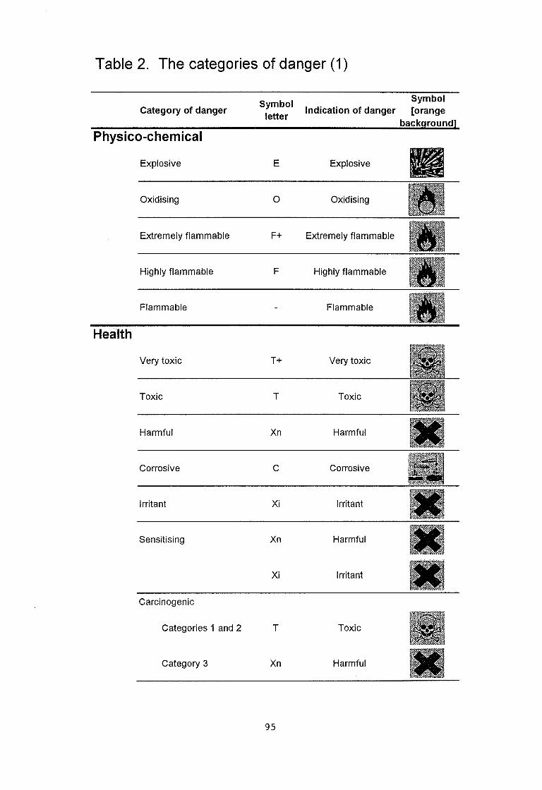
Table 2. The categories of danger (l)
S\~mhnl Categorv of danger
Symbol - -
IGLLGI backqround]
Physico-chemical
Explosive Explosive
Oxidising 0 Oxidising
Extremely flammable F+ Extremely flammable
Highly flammable F Highly flammable
Flammable
Health
Very toxic
Toxic
Harmful Harmful
Corrosive C Corrosive
Irritant
Sensitising
Carcinogenic
Categories 1 and 2 T
Category 3 Xn Harmful

Table 2. The categories of danger (2)
Symbol Symbol
Category of danger letter Indication of danger [orange background]
Mutagenic
Categories 1 and 2 T
Category 3 Xn Harmful
Toxic for reproduction
Categories 1 and 2 T
Category 3 Xn Harmful

Table 3. General guidelines for determining toxicological hazard categories (after EC Directive 931211EEC)
Hazard Classification of Substances with Risk Numbers
SPECIAL Carcinogenic; mutagenic; toxic to reproduction; R45, R46, R49, R60, R61. Respiratory sensitisers; R42.
HIGH
MEDIUM
LOW
Very toxic; R26, R27, R28. Toxic; R23, R24, R25, R48. Skin sensitisers; R43. Corrosive; R34, R35.
Harmful; R20, R21, R22, R48.
Substances examined but not meeting the criteria of the other hazard categories
Table 4. Advantages and disadvantages of animal data in Risk Assessment
Advantages Exposure - effect relationship usually clear and relatively easily determined. (Cause and effect made clear)
o Absence of confounders.
Disadvantages o How relevant are studies on animals to humans? o How relevant are studies with high doses to the response from low doses?
Normally the animal population is very homogeneous in contrast to the heterogeneity of the human population.

Table 5. Procedure followed in the determination of human Predicted No Adverse Effect Levels (PNAEL) and their modification by scientific uncertainty or "safety" factors*.
Exposure
Hazard
Critical Effect
Short-term repeated1 SubchroniclChronic Extrapolation LOAEUNOAEL Extrapolation
Route-to-route extrapolation
lnterspecies variability
lntraspecies variability
Human PNAEL(s)
Degree of confidence1 scientific uncertainty
Review exposure database - establish route(s) and patterns of exposure and define human PNAEL's required Review hazard database - decide whether adequate starting point exists for derivation of the required PNAEL's. If so, proceed; if not, recommend that risk management be considered. Identify critical effect(s) and establish NOAEL(s) or LOAEL(s) Consider need for and determine size of factor to take account of short-term repeatedlsubchroniclchronic extrapolation In the event that NOAEL(s) have not been established, determine value of factor(s) required to extrapolate from LOAEL(s) to NOAEL(s) If the experimental data have been generated by a route of administration other than that relevant to the human exposure situation. consider validity of route-to-route extrapolation and, if valid, calculate equivalent NOAEL by relevant route In the event that the hazard data are derived from animals, determine the validity of interspecies extrapolation and the value of the factor required to take account of differences between experimental animals and man Determine the value of the factor required to take account of human variability in response to toxic chemicals Using the overall adjustment factor derived by multiplying together the factors determined in steps 4 to 8, derive the appropriate human PNAEL(s) from the starting LOAEL(s) or NOAEL(s) Consider the degree of scientific uncertainty inherent in each of the above stages and decide whether the overall confidence in the derived human PNAEL(s) is "High", "Medium" or "Low"
p-
* European Centre for Ecotoxicology and Toxicology of Chemicals (1 995) Assessment Factors in Human Health Risk Assessment (Technical Report No. 68), p. 41-42. Brussels: ECETOC.

Table 6. An example of a Risk Assessment Worksheet using the ECETOC Procedure*.
Review of Data Base
Exposed population: Route of exposure: Pattern of exposure (single dose, intermittent, continuous): Human PNAEL(s) required: Critical effect(s): Pivotal studylstudies: NOAEL or LOAEL (A):
Adjustment Factors Occupational Non-Occupational
Exposure Exposure Default Applied Default Applied Value Value Value Value
Short-term repeatedlsubchroniclchronic extrapolation: short-term repeated to subchronic 3 3 subchronic-chronic 2 - 3 2 - 3
LOAEL - NOAEL 3 3
Route-to-route -
Interspecies extrapolation: oral 4 4 inhalation 1 1
lntraspecies variations 2 3
Overall Adjustment Factor (B)
Human PNAEL (AIB)
Degree of Confidence
Recommendations:
* European Centre for Ecotoxicology and Toxicology of Chemicals (1995) Assessment Factors in Human Health Risk Assessment (Technical Report No. 68), p. 43. Brussels: ECETOC.
99

Fig. 1. Progressive changes occurring when an organism is challenged with increasing doses of a toxic substance
initial normal state -L
homeostatic adjustment -L
compensation (input of reserve capacity with possibility of repair)
-L breakdown
(leading to increased disability and, ultimately, death)

Fig. 2. Procedure proposed by WHO for the derivation of uncertainty factors in the extrapolation from a toxicity data base to a tolerable intake
world Health Organization (1994)l Assessing Human Health Risks of Chemicals: Derivation of Guidance Values for Health-based Exposure Limits. International Programme on Chemical Safety Environmental Health Criteria 170, p. 33. Geneva:WHO.
I SELECTION OF PIVOTAL STUDY 1 I AND CRITICAL EFFECT l'
I l .L
ADEQUACY OF PIVOTAL STUDY I
L FROM ANIMAL DATA
I
INTER-SPECIES INTER-SPECIES TOXICODYNAMICS TOXICOKINETICS
2.5 (1 0 Oe4 ) 4.0 ( l 0 0-6 )
IN TOXICODYNAMICS IN TOXICOKINETICS
NATURE OF TOXlClTY 1 OVERALL DATABASE 1 DATA OVERVIEW +
1 UNCERTAINTY FACTOR I

Fig. 3. The Benchmark Dose
Upper confidence limit-. Excess on estimated risk - - '
proportion of abnormal responses
Dose-response fitted 0. l
to experimental data
0.11F
0 LED,dF LEDl0 EDIO Dose

Air
Soi
Surface - water PEOPLE
Ground , water
Drinking water Fig. 4. Potential exposure routes in assessing exposure to the general public

Fig. 5. Hierarchy of control measures
Prevention a Elimination a Substitution a Good Hygiene Practice
Physical segregation a Complete enclosure with extraction e Local exhaust ventilation with or without partial
enclosure a Screening
Personal protection e Respiratory protective equipment
Respirators - Self-contained breathing apparatus
a Protective clothing (eye and head protection, gloves, shoes, apronloveralls, etc)


UNEPIIPCS Training Module No. 3
Section B
Environments Assessment


UNEPIIPCS TRAINING MODULE SECTION B
ENVIRONMENTAL RISK ASSESSMENT
TABLE OF CONTENTS
EDUCATIONAL OBJECTIVES ......................................................................... 112
1 THE GENERAL ASSESSMENT SCHEME ................................................. 112 ..................................................................... l I Exposure assessment 112
1.2 Effects assessment ......................................................................... 113 ....................................................................... 1.3 Risk characterization 113
......................................................... 1.4 Risk estimation and reduction 113
........................................................................ 2 EXPOSURE ASSESSMENT 114
2.1 Water .............................................................................................. 114 ........................................................ 2.1 . 1 Point source releases 114
..................................................... 2.1.2 Diffuse source releases 115 .................................................................. 2.1.3 Biodegradation 115
............................................. 2.1.4 Physico-chemical properties 116 2.1.4.1 Solubility ........................................................... 116 2.1.4.2 Volatility ............................................................. 116
2.1.4.3 Hydrolysis ............................................................ 116
2.1.4.4 Photolysis .......................................................... 116 ........................................................... 2.1.4.5 Adsorption 117
............................................................. 2.1.5 Mackay modelling 117 ................................................................... 2.1.6 Bio-availability 117
......................................................................................... 2.2 Sediment 117 ................................................................ 2.2.1 Mode of release 117
............................................................. 2.2.2 Mackay modelling 118 ................................................... 2.2.3 Degradation in sediment 118
................................................................................................... 2.3 Air 118 ..................................................................... 2.3.1 Use category 118
............................................................................. 2.3.2 Volatility 118 ............................................................. 2.3.3 Mackay modelling 119

.................................................. 2.3.4 Atmospheric degradation 1 19 .............................................. 2.3.5 Rain-out and dry deposition 119
2.3.6 Industry specific information .............................................. 120 .................................................................................................. 2.4 Soil 120
.................................................... 2.4.1 Sewage sludge disposal 120 2.4.2 Rain-out and dry deposition .............................................. 120
............................................................. 2.4.3 Mackay modelling 120 .................................................................. 2.4.4 Biodegradation 120
2.4.5 Leachability ....................................................................... 121
2.5 Biota ................................................................................................ 121 ................................................................... 2.5.1 Uptake by fish 121
2.5.2 Uptake by plants ............................................................... 121 ................................ 2.5.3 Uptake by worms or other organisms 121
2.5.4 Uptake via the food chain .................................................. 122 ............................................ 2.6 Use of environmental monitoring data 122
............. 2.7 Indirect exposure to humans from environmental sources 123 ................................................................... 2.7.1 Drinking water 123
.................................................................................. 2.7.2 Food 124
3 EFFECTS ASSESSMENT ........................................................................... 125 ............................................................ 3.1 Aquatic effects assessment 125 .......................................................... . 3.1 1 Acceptability of data 125
3.1.2 Assessment factors and the calculation of PNEC ............. 126 ...................................................... 3.1.3 Future testing strategy 130
......................................................... 3.2 Sediment effects assessment 130 .......................................................... 3.2.1 Acceptability of data 130 ........................................................... 3.2.2 Assessment factors 131
...................................................... 3.2.3 Future testing strategy 131 3.3 Air effects assessment .................................................................... 131
3.4 Soil effects assessment .................................................................. 132 3.4.1 Acceptability of data .......................................................... 132
........................................................... 3.4.2 Assessment factors 132 ...................................................... 3.4.3 Future testing strategy 132
............................................ 3.5 Assessment of contamination of biota 133
.......................................................... 3.5.1 Acceptability of data 133 ........................................................... 3.5.2 Assessment of data 133

4 BIBLIOGRAPHY ........................................................................................... 134
.................................................... 5 SELF ASSESSMENT QUESTIONS 135
ANNEX 1 . Example of test requirements for new chemicals used for
chemicals notification and hazard assessment in some countries . Base set ........................................................................................................ information 136
ANNEX 2 . Predicted environmental concentration (PEC) in water .................. 142
ANNEX 3 . Notes on bio-availability and biological 1 environmental monitoring 148
ANNEX 4 . Assessment of environmental distribution . the use of fugacity models for this purpose ................................................. ................................. 151
ANNEX 5 . Exposure assessment for drinking water ....................................... 166
............................................................. ANNEX 6 . Adsorption onto sediments 170
ANNEX 7 . Bioconcentration in fish .................................................................. 172
ANNEX 8 . Dietary intake figures ................................................................ 173

UNEPllPCS TRAINING MODULE
SECTION B
ENVIRONMENTAL RISK ASSESSMENT
EDUCATIONAL OBJECTIVES
You should understand the use of predicted environmental concentration and
predicted no effect concentration in environmental risk assessment. You should
also understand the relationship to risk characterization and risk management. The general principles involved in relating release of substances to exposure to biota
and humans should be understood, including the significance of physico-chemical principles and bio-availability. The assumptions and uncertainties behind
assessment factors must be understood. Problems should be identified as a basis
for future improvements in risk assessment.
l THE GENERAL ASSESSMENT SCHEME
Using the relevant data, a predicted environmental concentration (PEC) and a
predicted no effect concentration (PNEC) for each environmental compartment are
assessed. If the PEC exceeds the PNEC, there is considered to be risk of environmental damage in proportion to the ratio of PEC to PNEC. This approach is
the one most favoured at present but, in spite of being developed in great detail,
especially by the European Commission, it is somewhat simplistic and further
development to take better account of ecosystem complexity (see the section on
Ecological Risk Assessment) is to be expected.
I I Exposure assessment
The PEC is calculated initially using realistic worst case scenarios developed from
lndustry or Use Category Documents or, if these are not available, from estimated
figures. lndustry or Use Category Documents provide details of processes used by
various sectors of industry and try to quantify the releases from these processes for
various groups of substances.

Particular consideration should be given to the type of release (i.e. point source,
diffuse source, continuous release, semi-continuous or intermittent) as this has
important consequences for the duration and frequency of exposure of an ecosystem to a substance. If monitoring data are available, they should normally be
used in preference to calculation.
1.2 Effects assessment
Ecotoxicity data are used to develop a PNEC. If the PNEC is greatly exceeded in
the environment, adverse effects may follow. The PNEC value combines the ecotoxicity data with an assessment factor. This factor reflects the confidence in the
data. Details of the methods used to estimate the PNEC are given below in section 3.
1.3 Risk characterization
Risk characterization involves assessing risk by comparing the PEC with the PNEC.
If the PEC is greater than PNEC, this indicates that the substance may cause harm. The ratio of PEC to PNEC is taken as a measure of the probability that harm will occur.
l .4 Risk estimation and reduction
Quantification of the likelihood and severity of adverse effects resulting from the use of the substances of concern in various ways may indicate the nature of the controls necessary to reduce the environmental risks to an acceptable level.
Controls of point sources will generally conform to the principles of Best Available Techniques (BAT), while more diffuse sources should be controlled using Best Environmental Practice (BEP). BAT and BEP can involve a wide range of possible controls ranging from provision of information to substance users, through codes of
practice to regulatory controls. Controls will require a comparison of the risks and benefits associated with use of the substance of concern and any alternatives.
Control of one unacceptable risk should not lead to its replacement by another.

2 EXPOSURE ASSESSMENT
2.1 Water
This section considers exposures of aquatic organisms via surface waters. Exposure of humans and other mammals by drinking water is discussed in
section 2.7.
Various exposure scenarios are possible. These scenarios vary in the mode of release of the substance. The types of release can be broadly divided into two main
categories, diffuse source and point source. These can further be divided into
another two categories, dispersed and non-dispersed.
Point source releases are characterised by a small number of release points into a small geographical area. There may be only one such area of release, for example
the effluent from a substance manufacturing plant, or the areas of release may be widely distributed across the country, for example effluent from sewage treatment plants. These two examples could be termed point source non-dispersed and point
source dispersed releases respectively.
Diffuse source releases are characterised by many release points, which can either be in a locafjsed area (diffuse source non-dispersed), for example releases of substances from apple orchards, or from near motorways, or over a wide geographical area (diffuse source dispersed), for example vehicle exhaust emissions or agricultural run-off from arable land.
Another important consideration is the time pattern of the release. Continuous
release is likely to be much more harmful than intermittent or infrequent.release.
2.1 .l Point source releases
As an example of a point source release, we can consider a substance discharged
from a pipe into a river of given flow. For initial assessment, the river may be assumed to be of a "standard" size (usually 0.5 m3 1 S). In a more refined assessment, the actual site-specific size of river should be used. Examples of methods of calculation of PEC for point source discharges are shown in Annex 1. When estimating the PEC the factors discussed in sections 2.1.3 - 2.1.6 should be

taken into account. The environmental properties of possible breakdown products of the substance must also be considered.
2.1.2 Diffuse source releases
Diffuse source releases are characterised by a number of release points. Each individual source of release may be of a much lower level than those typically associated with point source release, but collectively they may add up to a significant release across a region. Diffuse sources generally make up the background equilibrium exposure to the substance.
Examples of methods of calculation of PEC for diffuse source discharges are shown in Annex 2. When estimating the PEC the factors discussed in sections 2.1.3 - 2.1.6
should also be taken into account.
2.1.3 Biodegradation
Biodegradation is potentially an important process for reducing the concentration of
a substance in water, both for releases directly to water and for releases via sewage treatment works.
Physical, chemical and biological processes as a consequence of sewage treatment may reduce the PEC. Information on the % removal of a substance during sewage treatment is needed in calculating the PEC (see Annex 2).
Further work is required in relating the biodegradability of a substance as measured
in the laboratory (and other processes such as adsorption, volatilisation etc.) to the amount of substance removed by sewage treatment.
Biodegradation continues once a substance is released to surface water.
For "end of pipe" emission estimates, the PEC calculated at the point of release will be maintained as long as the release rate remains constant (continuous release).
Biodegradation will affect the concentration downstream from the discharge. The concentration of a degradable substance should be markedly reduced downstream from the discharge by biodegradation and further dilution, whereas the concentration of a nondegradable substance can only be reduced by further dilution.

If a large amount of a readily biodegradable substance is likely to be released to a
watercourse, it may cause problems owing to depletion of oxygen. This will depend
on external factors such as the re-aeration rate of the water and the amount of plant
growth in the water.
2.1.4 Physico-chemical properties
2.1.4.1 Solubility
The solubility of a substance in water limits the theoretical maximum value of the
PEC. A substance will not be present in solution at a concentration above its
solubility, unless solubilized by other substances.
2.1.4.2 Volatilitv
Volatility affects the concentration of a substance once it is released into the
environment. Highly volatile substances (as indicated by the Henry's Law constant)
are likely to evaporate from water to the atmosphere. Thus, the PEC is reduced with
time (and distance) from the source of release.
The retention time of a substance in a sewage works and the aeration will both
facilitate volatilisation.
2.1.4.3 Hydrolysis
Hydrolysis is the breakdown process in which a substance reacts with water. The
rate of hydrolysis is dependent upon the pH of the water.
For substances which hydrolyse readily at normal pH values, the PEC will be
reduced with time (and distance) from the source of release.
2.1.4.4 Photolysis
Photolysis is the breakdown process of a substance in water activated by absorbed
light energy.
2.1.4.5 Adsorption
Adsorption onto sediment is can have a profound effect the PEC for water. A
method for predicting the effect of adsorption on the PEC is given in Annex 6.
2.1.5 Mackay modelling
Mackay modelling may not be relevant to point source releases to water as the
highest concentrations and highest likely concern will be associated with the initial
discharge.
Mackay modelling may be useful in estimating the likely final distribution of a
substance by giving an estimate of the effects of volatilisation, adsorption etc. on the
substance once released to water (see Annex 4).
Bio-availability depends upon the physical and chemical form of the substance
released. For organic compounds, fat solubility and water solubility are the key
properties.
Of particular importance for metals is the oxidation state, their ionization state in
solution, their interactions with chelating agents, and the physical form of release
(for example as a solution or as a suspension which may be removed by adsorption
and sedimentation etc.) (see Annex 3).
2.2 Sediment
The concentration of a substance can build up in sediment and the sediment can
then act as a source of the substance in water, even if the primary source of
discharge is removed. Where the substance has low water solubility and a high
bioconcentration potential (measured by octanollwater partition CO-efficient), flow of
the substance from sediment through water to organism may occur without the
substance reaching an analytically detectable level in the water.
An example of how the PEC for sediment can be estimated is given in Annex 6.

2.2.1 Mode of release
If a substance is released as a suspended solid, this could contaminate sediments
directly and lead to higher concentrations than may be predicted from equilibrium partitioning.
2.2.2 Mackay modelling
Mackay modelling is useful in predicting whether adsorption onto sediment is likely
to be a significant process or not. This multimedia approach takes into account other factors such as volatility etc. on the sediment sorption (see Annex 4).
2.2.3 Degradation in sediment
Both aerobic and anaerobic conditions may be found in sediments. If no sediment
specific degradation studies are available for a substance it may be possible to use data obtained in studies of degradation in water.
2.3 Air
In general, it is unlikely that the concentration of a substance in air will be high enough to cause toxic effects in the environment. An exception may be around point sources, where localised high concentrations may exist.
The following information may be useful in estimating if there is a harmful release to
air.
2.3.1 Use category
Substances can enter the air both deliberately and accidentally. For example,
propellants in aerosol sprays are deliberately released to air. On the other hand, benzene is accidentally released by evaporation from petrol at filling stations.
It is important for industry to produce release inventories in order to permit the amount of substance released to air to be calculated.

2.3.2 Volatility
Highly volatile substances (as indicated by their vapour pressure andlor Henrys Law constant) are likely to end up in the atmosphere even if they are originally released
to water or other media.
2.3.3 Mackay modelling
Mackay modelling is very useful for predicting if a large fraction of the total release of a substance is likely to end up in the atmosphere (see Annex 4).
2.3.4 Atmospheric degradation
If the substance has a very short atmospheric half-life, it will only occur in the lower
troposphere. However, long-lived substances may also occur in the stratosphere or be transported to parts of the globe far removed from the original source.
2.3.5 Rain-out and dry deposition
Substances released directly to air may be removed by rain. This can occur by dissolution in the rain water or by adsorption onto atmospheric particles, which in turn may be washed out by rain.
Substances can also be removed from the atmosphere by dry deposition. They can
be dry deposited directly or via adsorption onto airborne particulates which then
settle out of the air or are breathed in by animals and humans.
Gaseous pollutants may react with other substances to form particulates which can
in turn be dry deposited (e.g. oxidation of gaseous SO2 to particulate sulphates).
In predicting if these processes are likely to be significant, the Henry's Law constant
(a low value would indicate that the substance is likely to partition preferentially from
air into water) and KO, (high values would indicate that adsorption to organic rich
atmospheric particles such as soot, may be significant) and the application of the
fugacity approach may be useful (see Annex 4).

2.3.6 Industry specific information
Any information provided by an industry may be useful in trying to estimate the amount-of a substance released to air. In particular, information about production
schedules and amounts of material being processed at particular times may be a basis for quantitative estimates of emissions.
2.4 Soil
The following data may be useful for estimating the likelihood and significance of environmental exposure to a substance through the soil.
2.4.1 Sewage sludge disposal
Sewage sludge disposal to land could provide a source of exposure through soil for
certain substances if they are likely to be present. This may be the case for
substances with large sedimenusediment-water partition coefficients (or large Koc or
KO,) and which are not volatile or biodegradable (see section l .l .3).
2.4.2 Rain-out and dry deposition
If substances are likely to be present in rain water or adsorbed onto atmospheric
particles, this could provide a source of soil contamination (see section 2.3.5). For this to be a major source, the substance would have to be persistent in soil or have
a high flux into soil.
2.4.3 Mackay modelling
Mackay modelling is useful in estimating if a large fraction of the total release is
likely to end up in soil (see Annex 4).
2.4.4 Biodegradation
Both aerobic and anaerobic degradability are relevant for soils. Biodegradation varies enormously with the chemistry of soil and soil water. It also reflects the previous history of the soil that will have led to the selection of characteristic

microbial flora. If no soil-specific degradation studies are available for a substance it may be possible to use data obtained in studies of degradation in sediments or in
water, although in general soil has a greater biodegradation potential than water.
2.4.5 Leachability
Many substances that adsorb only weakly onto soil are free to leach from the soil
into ground water. This may be significant for substances with moderate to high
water solubility and relatively low soil-water partition coefficients (or low Koc or KO,).
2.5 Biota
2.5.1 Uptake by fish
If a measured bioconcentration factor (BCF) for a fish species is available, this can
be used to estimate the concentration expected in the fish exposed to a known
concentration of a substance in water (see Annex 7). If no BCF is available, a value
can be estimated for certain substances using QSAR methods (see section 3.1 .l).
Once an estimated concentration in fish has been obtained, this can be used along
with fish dietary intake figures to estimate an exposure for humans (see Annex 7).
2.5.2 Uptake by plants
If any information is available on the uptake of a substance by plants from water (for
example, a BCF for algae) or soil (for example, plant uptake data), this can be used
to estimate a concentration in the plant by a similar method to that in section 2.5.1,
using the appropriate PEC. For certain substances (e.g. dioxins), leaf surface
contamination from atmospheric deposition may be significant.
2.5.3 Uptake by worms or other organisms
If any information is available on the uptake of a substance by worms (for example,
a BCF measuring uptake via soil) or any other (for example, filter feeding) organism,
this can be used to estimate a concentration in the animal, resulting from the actual or estimated concentration in the soil, by a similar method to that in section 2.5.1,
using the appropriate PEC.

2.5.4 Uptake via the food chain
If it has been possible to calculate a level of a substance expected in biota (sections 2.5.1-2.5.3), this can then be used as a dose (mglkg) for animals further up the food chain (biomagnification), e.g. birds, fish-eating mammals and humans (Annex 8). The effects on humans are covered in Section A on human health risk assessment. Effects on other species are covered in section 3.5.
Metabolism controls the removal of a substance from an animal or plant species. It is particularly important to consider this process when using estimated BCF data. For measured BCF data, metabolism will have been occurring during the experiment
and so will be reflected in the BCF value obtained.
2.6 Use of environmental monitoring data
For certain substances, extensive environmental monitoring data may be available for the releases and concentrations found in environmental media. These data are
very useful in environmental exposure assessment and may be used alongside the PEC in the overall assessment and as "case studies" for checking model predictions.
Although due weight should be given to monitoring data, care must be taken in its
use, and the-following points should be considered (see also Annex 3):
1) the representativeness of the data.
2) the areaafrom which the measurements were taken and in particular whether the area is likely to represent an area of high contamination (for example, in the neighbourhood of a production site) or an area where more average contamination is possible.
3) the suitability of the analytical method used. This is particularly relevant if the detection limit is higher than the PNEC, as then a 'not detected' result is of little use. In addition the results must be evaluated in terms of whether concentrations have been quantified and reported as total residues or as fractionated concentrations of dissolved, bound or non-reactive substance.

Other types of monitoring data may also be useful in environmental exposure
assessment, for example amounts released from point sources and quantities and
volumes of releases to air etc. Such information would allow the PEC calculation to
be refined.
2.7 Indirect exposure to humans from environmental sources
Human health risk assessment requires the use of information on the indirect
exposure of humans from environmental sources of the substance.
Several authorities (e.g. RIVM, USEPA) have developed methodologies for
calculating substance-specific human intakes for discrete environmental pathways.
Described below is the general approach adopted in the RIVM method for calculating the total human dose from water, soil and other sources. When using
this method, the risk assessor must realise that the calculated dose is expressed as
the amount of the substance at the body's exchange boundary (e.g. skin, gut or
lungs) and available for adsorption, not necessarily the amount reaching the target
tissue.
The underlying basis for estimating human exposure by any environmental route is
to multiply the measured or predicted concentration in the medium being assessed
(e.g. water, fish, meat, milk, or air) by the estimated human daily intake of the
medium.
Estimates of human daily intake should be protective of sub-populations that may be
at greater risk (i.e. children, elderly).
2.7.1 Drinking water
A method for estimating the concentration of a substance in drinking water is given
in Annex 4.
The daily dose (mg l kg b.w.) for a human from drinking water can be estimated from
the concentration in drinking water, assuming an average body weight of 60 kg and a daily water intake of 2 litreslday. For other mammals, which may drink
contaminated water, a similar approach can be used. However, it must be realised that there can be extreme variations around these values, particularly among young
people who may adopt unusual diets, frequently involving a much larger water intake.
2.7.2 Food
A method for estimating a daily human dose from eating fish is outlined in Annex 8.
Methods for estimating doses from other foods, including plants, can be found in the
RlVM Report "A Shorthand Method: Predicting the Indirect Exposure of Man".

3 EFFECTS ASSESSMENT
There are many proposed methods for carrying out effects assessments (e.g. OECD, see section 4). Most of the methods apply the same general principles; they
use the available toxicity data to derive a L(E)C,,, a no observed effect concentration (NOEC) or a lowest observed effect concentration (LOEC) and then application of assessment factors (or safety factors) to these data to obtain a
concentration above which the substance may cause harm (PNEC).
The size of the assessment factor varies according to the quality of the data available and the likely duration of the exposure. The assessment factor is intended
to extrapolate from the laboratory experiments to the 'real life' field situation. If
enough toxicity data are available, various extrapolation methods can be used to obtain a PNEC (see below). For some substances, Environmental Quality Standards (EQS) will have been set, for example - by the European Union through
daughter directives to Directive 761464lEEC or by national competent bodies. Where EQS are available, these should be considered before setting a PNEC.
Once a PNEC has been established, it is compared with the relevant PEC. If the PEC > PNEC, this indicates that harmful effects may occur. Further information may
then be required to refine both the PEC and PNEC. If the PEC is still greater than the PNEC, this indicates that risk estimation and risk reduction steps should be considered.
Below are the types of data to be considered in estimating the PNEC and how this may be used with the appropriate PEC.
3.1 Aauatic effects assessment
3.1 .l Acceptability of data
Toxicity tests should preferably follow the accepted methods (e.g. described by EU, OECD or ISO) and carried out to GLP. Other 'non-standard' tests may be used if they are carried out to an acceptable standard. Particular attention should be given to whether measured or nominal concentrations are used.
It should always be borne in mind throughout the assessment that the toxicity data are being used to estimate the concentration in water above which toxic effects may

occur. In order to do this reliably, it is essential to know the actual concentration in solution that the test species were exposed to. This is particularly relevant to substances that may be unstable, adsorb onto the test vessel or volatilise through the test period.
Quantitative structure activity relationships (QSAR) may be useful for certain types of substances where there are few or no data available. Toxicity estimates from QSAR models can provide useful surrogate data for effects assessments, but there are numerous restrictions that apply to their use. An evaluation of the likely mode of
toxic action of the substance must be carried out before a suitable QSAR model can be selected. QSAR predictions should be evaluated to ensure that the results are consistent with what is known for substances of similar structure and mode of toxic action.
All types of aquatic toxicity data should be considered in the assessment. For data
of an acceptable quality, chronic study data should be used in preference to acute data if there is likely to be long-term exposure to the substance, but if exposure is intermittent then acute data should be used. Actual acute or chronic data are always preferable to data predicted from QSAR or derived from assessment factors.
Ideally, data for three different taxonomic groups should be considered, usually represented by a fish species, Daphnia, and an alga. For conservative assessment
purposes, data from the most sensitive species should be used in extrapolations from laboratory data to ecosystem effects assessments.
It should be noted that in the case of algal studies, which are actually multi-
generation studies, there is broad acceptance that a 72 hour ECn value may be
cansidered as equivalent to an acute result and that a 72 hour NOEC value may be
considered as a chronic result.
3.1.2 Assessment factors and the calculation of PNEC
The purpose of assessment factors is to allow extrapolation from laboratory toxicity test data to ecosystem effects. It is assumed that:
1) although ecosystem sensitivity is a complex attribute, it can be approximated to the sensitivity of the most sensitive species (for localised discharges, consideration

must be given to site-specific sensitive species);
2) protection of community structure (e.g. species list, diversity, size- and age-class) ensures protection of ecosystem function (for example, fixation and transfer of energy, productivity, resistance to perturbation, recycling of nutrients);
3) by establishing the most sensitive species to the toxic effects of a substance in
the laboratory, extrapolation can subsequently be based on data from that species;
4) the functioning of any ecosystem in which that species exists is protected provided that the ecological structure is not distorted. The working but arbitrary hypothesis is that protection of the most sensitive species with a 95% confidence limit should protect ecosystem structure and hence function.
For most existing substances, the pool of data from which to predict ecosystem effects is very limited. In many cases, only single-species acute toxicity data are
available. In these circumstances, it is recognised that, while not having a strong scientific validity, empirically derived assessment factors must be used. In applying
such factors, the intention is to predict a level at or above which the balance of probabilities suggests an environmental effect may occur. It is not necessarily a
level below which the substance is considered safe but the balance of probability is that there will be no effects.
In establishing assessment factors, a number of uncertainties must be addressed which are inherent in attempting to extrapolate from single species laboratory data to multi-species ecosystems. These may be summarised as follows:
1) Inter-species variations
2) Acute to chronic toxicity extrapolation
3) Extrapolation from laboratory data to safe levels in the field
4) The testing methods.

To calculate a PNEC from the available data, the experimentally determined no
observed effect concentration (NOEC) is divided by an assessment factor selected
according to the strength of the available data as follows
Assessment Factor
(a) Acute toxicity data from more than l000 (Note l)
one species (applied to the lowest L(E)C,,)
in place of NOEC)
(b) Chronic toxicity data where data are
not necessarily from the most sensitive species (applied to the species lowest NOEC)
(c) Chronic toxicity data based on data from the most sensitive species (applied to the lowest NOEC)
50 (Note 2)
10 (Note 3)
(d) If the field data exist, they will need
to be reviewed case by case.
Note 1 The use of a factor of 1000 on acute data is a highly conservative and .protective factor and it should be noted that this factor is at variance with a factor of
l 00 used by the US EPA and a factor of 200 derived by ECETOC. Thus, the proposed factor of 1000 is designed to ensure that all substances with the potential to cause adverse effects are identified in the assessment. It assumes that each of
the above identified uncertainties makes a significant contribution to the overall uncertainty. For any given substance there may be evidence that this is not so, or
that any given component of the uncertainty is more important than any other. In these circumstances, it may be necessary to vary this factor. Evidence in support of a reduced factor could include one or more of the following:
(i) information to suggest that the lowest L(E)C50 is from a group which is likely to represent the most sensitive species (not just the most sensitive
tested);
(ii) information, from structurally similar compounds or elsewhere, to suggest that the acute to chronic toxicity ratio is likely to be low;

(iii) information to suggest that the substance acts in a non-specific or narcotic manner, with little inter-species variation in toxicity;
(iv) information to suggest that the substance's release would be short-term
and intermittent and would not persist in the environment.
(v) any other information that would suggest that a lower assessment factor
would be appropriate.
Note 2 An assessment factor of 50 will normally be applied when only one or two chronic NOECs have been determined from different taxonomic groups. This will usually mean from either fish or Daphnia together with an algal toxicity NOEC. This may be reduced to 10 if there is evidence that the most sensitive species has been
tested.
Note 3 An assessment factor of 10 will normally only be applied when chronic
toxicity NOECs are available from three species across three taxonomic groups (i.e.. fish, Daphnia, and algae). If there is evidence that the most sensitive species has been tested, the factor may be applied to the lowest value from two species.
Application of an assessment factor in deriving a PNEC and subsequent comparison
to a Predicted Environmental Concentration (PEC) will produce a number of substances for which additional information will be required. Such additional information .may lead to a revision of the PEC, of the PNEC, andlor of the
assessment factor.
Any review of the initial risk characterisation requires close co-operation between the reviewers and industry. It is at this point that a discussion of the assessment factor can take place, but it must be made clear that the onus will be on the manufacturer or supplier to justify a lower factor and support this with the necessary data.
When examining the results of chronic data, where possible, the PNEC should be calculated from the lowest available No Observed Effect Concentration (NOEC). Extrapolation to ecosystem effects can be made with greater confidence, and thus a significant reduction in the assessment factor is possible.
In moving from laboratory tests to ecosystems, an assessment factor of 10 is
applied to the NOEC from chronic studies. This is only sufficient, however, if the
species tested can be considered to represent one of the most sensitive groups. This would normally only be possible to determine if data was available on at least
three species across three taxa.
It may sometimes be possible to determine that the most sensitive species has been examined, i.e., that a further chronic NOEC from a different taxonomic group would
not be lower than the data already available. In those circumstances, a factor of 10
applied to the lowest NOEC would also be appropriate. This is particularly important if the substance does not have a potential to bio-accumulate (i.e. does not have a log Kow of more than 3). If it is not possible to reach this conclusion, an assessment
factor of 50 should be applied to allow for any interspecies variation in sensitivity. An algal study NOEC is not considered to extrapolate to other species. Thus, an
assessment factor of 50 would generally be applied if an alga were the only species
tested.
The assessment factor to be used on mesocosm studies or field data must be chosen on a case by case basis.
3.1.3 Future testing strategy
If the PEC > PNEC, this indicates that adverse effects may be caused by the substance in the environment. If this is the case, further information may be required, firstly, to refine the PEC calculation and, secondly, to refine the PNEC by further testing.
3.2 Sediment effects assessment
3.2.1 Acceptability of data
Unlike the aquatic toxicity tests, no agreed test guidelines exist for sediment toxicity, both with regard to species and methods. Information that may be useful could
include toxicity to worms and filter feeders. If any relevant information is available, this should be used in a similar way to aquatic data, using the PEC calculated for sediment.
The toxicity of sediment-bound substances to benthic biota is largely dependent on bio-availability. Sediment concentrations can be converted to a bio-available

fraction in pore-water using sediment-water partition coefficients. These pore-water concentrations can be used to determine potential effects on biota based on
standard test data. The possibility of enhanced exposure due to consumption of
contaminated sediment or direct physical contact with contaminated sediment has not been substantiated so far but is highly probable for some organisms.
In most cases, benthic species such as worms and bivalves are less sensitive than crustaceans and larval fish used in aqueous testing. Toxicity is reported to be reduced in sediments so that levels harmful in the overlying water may have no effects on the same species and life-stage in the sediment. Thus, sediment toxicity limits based on the pore water concentrations and standard species data sets are
believed to provide conservative and protective assessments for benthic species.
Additional test data should not be required for preliminary risk assessments. However for more detailed assessments, benthic species may need to be tested.
3.2.2 Assessment factors
Appropriate assessment factors must be developed once test guidelines have been
agreed (see Section 3.1.2).
3.2.3 Future testing strategy
If testing methods can be developed, exposure assessment carried out for sediment
(section 2.2) will highlight substances for which testing may be needed. Setting a trigger level for all substances in sediment may be a useful starting point. Thus, if the concentration of a substance were predicted to exceed a certain level in sediment, this would indicate that further work on exposure and effects of the substance in sediment is needed.
3.3 Air effects assessment
With exposure in air, it has been suggested that the only significant effects to be considered should be physical effects (human health effects are important but
usually considered separately). The physical effects to be considered for substances released in large quantities to air are:

- ozone depletion - global warming
- photochemical ozone creation potential (POCP) long-range transport of persistent pollutants that may lead to contamination of distant environments such as the Arctic
3.4 Soil effects assessment
3.4.1 Acceptability of data
The main types of data that are likely to be available to assess the effects of the substance on soil organisms include toxicity to worms, higher plants, and microbial
processes. Again, like sediment toxicity, it may be the soil pore-water concentration of a substance that is important in assessing its toxicity (see section 2.4.1).
3.4.2 Assessment factors
Appropriate assessment factors will need to be developed to be applied to the
different types of toxicity data currently available and which may be developed in the future (see section 3.1.2 and below).
3.4.3 Future testing strategy
The major problem is how to use the data available. One approach would be to try to calculate the PNEC using similar guidelines to those for the aquatic toxicity. This would involve the use of assessment factors.
Another approach is to set trigger levels (soil concentrations) for substances based on the likely exposure rather than the effects. Once the concentration of a substance approaches this trigger level, further investigation into its effects would be
required.
Much work remains to be done, particularly with regard to the use of assessment factors, types of data needed, further testing strategies and how to confirm that a predicted problem actually exists in the environment.

3.5 Assessment of contamination of biota
3.5.1 Acceptability of data
The basis for assessment in biota is the predicted concentration calculated in section 2.5.1 in fish, plants and other animals. It is assumed that higher animals and humans eat these organisms, and so a dose (mglkg) for higher animals and
humans can be estimated from the daily intake of these organisms.
Data useful for effects assessment would come from feeding studies on (fish-eating) mammals and birds. It is unlikely that such studies will exist for many substances
and one must use data on any bird or mammal species from feeding studies and from oral toxicity studies. When using data from oral toxicity studies, the concentration predicted in the food (fish, worms, plants etc.; see section 2.5) will have to be converted to the dose received by the animal (in mglkg body weight/ day)
by assuming a standard rate of feeding by the animal (see Annex 8).
3.5.2 Assessment of data
Initial assessment involves comparing the expected exposure of an animal in feed (PEC) with the concentration in feed that is thought to cause no effects in the animal (PNEC). Further work needs to be carried out in the following areas.
extrapolation of substance dose-response data from studies conducted with standard test species of birds or small mammals to determine risk to other water fowl and fish-eating birds and mammals
- derivation of assessment factors to be applied to the data
- derivation of factors to convert potential exposures to actual doses based on ecological information for bird and mammal species food consumption rates, food preferences, and food assimilation efficiencies

4 BIBLIOGRAPHY
Organization for Economic Cooperation and Development (1 992). Guidance for initial hazard assessment of High Production Volume (HPV) chemicals (aquatic effects assessment). Paris: OECD.
Lyman, W J, Reehl, W F and Rosenblatt, D H ( l 982). Handbook of Chemical Property Estimation Methods. New York: McGraw-Hill.
European Centre for Ecotoxicology and Toxicology of Chemicals (1 993).
Environmental Hazard Assessment of Substances (ECETOC Report No 51). Brussels: European Centre for Ecotoxicology and Toxicology of Chemicals.
European Commission (1 996). Technical Guidance Document in Support of Commission Directive 93167lEEC on Risk assessment for New Notified Substances
and Commission regulation (EC) No I488194 on Risk Assessment for Existing Substances (4 volumes). Luxembourg: Office for Official Publications of the
European Communities.

5 SELF ASSESSMENT QUESTIONS
What do the abbreviations PEC and PNEC stand for?
What are the main types of release affecting calculations of PEC? What is risk characterization?
What do the abbreviations BAT and BEP stand for? List possible scenarios for release of substances to water.
What is the relevance of biodegradation to risk assessment? How may the physicochemical properties of a substance affect the predicted environmental concentration?
What factors affect the concentration and bio-availability of substances in sediment? What factors affect the concentration and bio-availability of substances in air? What factors affect the uptake of substances by biota?
How does monitoring relate to uptake of substances by biota? In general terms, how may you estimate human exposure to environmental substances through food and drink? In general terms, how may the PNEC be calculated?
What are 'assessment factors' and how are they determined? What assumptions and uncertainties are involved? What evidence might justify reduction of an assessment factor?
What are the problems involved in sediment, soil and air effects assessment? How may the effects of contamination of biota through food webs be
assessed?

ANNEX l. Example of test requirements for new chemicals used for
chemicals notification and hazard assessment in some countries. Base set information.
l. IDENTITY OF THE SUBSTANCE
1.1 Name 1 . l . l Names in the IUPAC nomenclature
1 .l .2 Other names (usual name, trade name, abbreviation)
1 .l .3 CAS number (if available)
1.2 Empirical and structural formula
l .3 Composition of the substance 1.3.1 Degree of purity (%)
1.3.2 Nature of impurities, including isomers and by-products
1.3.3 Percentage of (significant) main impurities
1.3.4 If the substance contains a stabilising agent or an inhibitor or other additives,
specify: nature, order of magnitude: . . . ppm; . . . %
1.3.5 Spectral data (UV, IR, NMR)
1.4 Methods of detection and determination A full description of the methods used or the appropriate bibliographical
references
2. INFORMATION ON THE SUBSTANCE
2.1 Proposed uses 2.1 .l Types of use
Describe: the function of the substance
the desired effects
2.1.2 Fields of application with approximate breakdown
(a) closed system
- industries - farmers and skilled trades
- use by the public at large

(b) open system - industries. - farmers and skilled trades
- use by the public at large
2.2 Estimated production andlor imports for each of the anticipated uses or fields of application
2.2.1 Overall production andlor imports in order of tonnes per year 1, 10, 50 100; 500; 1,000 and 5,000
- first 12 months - thereafter
2.2.2 Production and/or imports, broken down in accordance with 2.1 .l and 2.1.2,
expressed as a percentage - first 12 months - thereafter
2.3 Recommended methods and precautions concerning: 2.3.1 handling 2.3.2 storage 2.3.3 transport 2.3.4 fire (nature of combustion gases or pyrolysis, where proposed uses justify 2.3.5 other dangers, particularly chemical reaction with water
2.4 Emergency measures in the case of accidental spillage
2.5 Emergency measures in the case of injury to persons (e.g. poisoning)
3. PHYSICO-CHEMICAL PROPERTIES OF THE SUBSTANCE
3.1 Melting point
3.2 Boiling point ...o C at ... Pa

3.3 Relative density (D420)
3.4 Vapour pressure - Pa at ..OC
3.5 Surface tension Nlm ( . X )
3.6 Water solubility mgllitre (. .OC)
3.7 Fat solubility Solvent-oil (to be specified) mgl100 g solvent (. .OC)
3.8 Partition coefficient n-octanollwater
3.9 Flash point . . .oC. open cup and closed cup
3.10 Flammability
3.1 l Explosive properties
3.1 3 Oxidizing properties
4. TOXICOLOGICAL STUDIES
4.1 Acute toxicity 4. l. 1 Administered orally
LDS0 mglkg Effects observed, including in the organs

4.1.2 Administered by inhalation
LC50 (ppm). Duration of exposure in hours Effects observed, including in the organs
4.1.3 Administered cutaneously (percutaneous absorption) LD50 mg/l Effects observed, including in the organs
4.1.4 Substances other than gases shall be administered via two routes at least one of which should be the oral route. The other route will depend on the
intended use and on the physical properties of the substance. Gases and volatile liquids should be administered by inhalation (a minimum period of
administration of four hours). In all cases, observation of the animals should be carried out for at least 14 days. Unless there are contraindications, the rat is the preferred species for oral and inhalation experiments. The experiments in 4.1 . l , 4.1.2 and 4.1.3 shall be carried out on both male and female
subjects. 4. 1.5 Skin irritation
The substance should be applied to the shaved skin of an animal, preferably
the albino rabbit. Duration of exposure in hours
4.1.6 Eye irritation The rabbit is the preferred animal.
Duration of exposure in hours 4.1.7 Skin sensitization To be determined by a recognized method using the
guinea-pig.
4.2 Sub-acute toxicity 4.2.1 Sub-acute toxicity (28 days)
Effects observed on the animal and organs according to the concentrations used, including clinical and laboratory investigations
Dose for which no toxic effect is observed
4.2.2 A period of daily administration (five to seven days per week) for at least four weeks should be chosen. The route of administration should be the most
appropriate having regard to the intended use, the acute toxicity and the physical and chemical properties of the substance. Unless there are contra- indications, the rat is the preferred species for oral and inhalation experiments.

6.2.3 Possibility of destruction:
- controlled discharge
- incineration
- water purification station
- others

ANNEX 2. Predicted environmental concentration (PEC) in water
A2.1 The two scenarios
1. Point source discharges This scenario assumesathe discharge is made direct to surface water. For a 'point source' discharge, it is assumed that there is essentially no contribution from other
point source discharges of the same substance.
2. Diffuse or widespread discharges This scenario covers situations where the discharge is genuinely diffuse (for example, loss from a widely used manufactured article) or discharge from multiple
point sources where the discharge may contribute to another discharge (for example, household detergent components).
A2.2 Estimation of emission of substances
It is essential to obtain as accurately as possible the emission pattern of a substance. This information can be based on:
- industry documents which give data on emissions from manufacture and use of substances;
- limited information obtained from analogous processes etc.;
- use of marketed tonnage, per capita usage of the substance, and other relevant data.
If the emission rate E (kg 1 d) and the volume of effluent Vo (m3 1 d) is known, then
the concentration (C) of the substance in the effluent is given by:

The emission rate E may be reduced to E l as a result of degradation D (D = percentage removed during treatment) etc. in which case the concentration
(Cl) is given by:
C1 = (Ex 103) (100 - D) /Vox l00 = E X 10 (100- D)/Vo mg / L [A2.2.2]
A2.3 PEC from point source discharge (AI)
For a point source directly discharged to a surface water, the concentrations C or C1 obtained in equations A2.2.1 or A2.2.2 above will be reduced by the dilution (added
volume) available from the receiving water.
Thus if this is Q m3/d then, for example, equation A2.2.1 becomes:
The above estimations assume that discharges direct to surface waters are instantly and completely mixed with the receiving water. For discharges to slow moving
bodies of water this assumption should not be made. In any case, for a first estimate of environmental concentration this assumption can be made. It may also be used for more accurate estimates of flow and distribution models if appropriate hydrological data are available to justify it.
A2.4 Refinina the PEC
A thermal paper chemical has two sources of release. The following scenarios may be applied.
l. Wastage at the Mixing and Coating Stage
This scenario assumes that wastage at the weighing and adding stages will be carefully controlled, and that any wastage will occur at the end of the thermal paper production cycle, when the mixing and coating vessels are washed out in preparation for a new cycle. It assumes that the chemical is added to a mixing vessel along with a range of other chemicals. After mixing, a suspension is formed in solvent and this is pumped into a coating tank, through which the paper passes. Excess reagent will be pumped away for reuse or controlled disposal. The vessels will be washed using water, and the washings passed to the wastewater.

Release via wastewater
The following data is thus used for the purposes of this model.
i) Batch size
ii) % in coating mixture iii) % Wastage from coating vessels
iv) Site waste water flow
v) % Removal by absorption I biodegradation vi) Flow rate of receiving waters
5 tonnes I day 13 %
3 % l00 m3 1 day
90 % 435 000 m3 1 day
Crude Effluent Concentration (EC) = li) X (ii) X (iii)
(iv) = 5.0 X l o g X 0.13 X 0.03 mg1L
I X i o 5
This effluent passes through a wastewater treatment where it can be assumed that 90% will be removed by absorption on the sludge. This waste then flows to a river of flow 435,000 m3 l day.
PEC =(i)x(i i )x( i i i )x(v)
( v i )
The assumptions used in the above calculations must be justified, by e.g. by
obtaining information from the notifier and water companies.
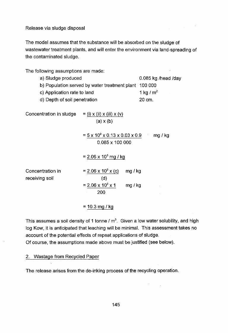
Release via sludge disposal
The model assumes that the substance will be absorbed on the sludge of
wastewater treatment plants, and will enter the environment via land-spreading of
the contaminated sludge.
The following assumptions are made:
a) Sludge produced 0.085 kg /head /day
b) Population served by water treatment plant l 00 000 c) Application rate to land l kg/m2
d) Depth of soil penetration 20 cm.
Concentration in sludge = (i) X (ii) X (iii) X (v)
(a) X (b)
Concentration in
receiving soil
= 2 . 0 6 ~ 103x (c) mg/ kg
(d) =2 .06x103x1 mglkg
200
This assumes a soil density of 1 tonne / m3. Given a low water solubility, and high
log Kow, it is anticipated that leaching will be minimal. This assessment takes no
account of the potential effects of repeat applications of sludge. Of course, the assumptions made above must be justified (see below).
2. Wastage from Recycled Paper
The release arises from the de-inking process of the recycling operation.

Release through wastewater
The following assumptions are made:
- i) Annual production
ii) % recycled via office waste iii) De-inking efficiency
iv) Absorption on solid waste v) No. of recycling plants
vi) No. of countries using paper. vii) Waste water uselsite viii) No. of days recycling
120 tonnes 10%
100% 90%
4 / country 6
8 000 m3 l day 300 days / annum
E C = (i) X (ii) X (iii) X (iv) mg / L (v) X (vi) X (vii) X (viii)
EC" = 120 X 109x 0.1 X 1.0 X 0.1 m g / ~
4 x 6 ~ 8 ~ 1 0 6 ~ 3 0 0
The assumptions can be justified as follows:
1) lnformation from the notifier.
2) lnformation contained in a use category research report. 3) Worst case assumption used for modeling purposes.
Release via sludge disposal
The model assumes that the substance will be absorbed on the sludge during clarification of the recycled wastewater and will enter the environment by land-
spreading of the contaminated sludge.
The following assumptions are made: a) Sludge produced / tonne of paper 5% w/w b) Tonnage of paper produced 130 tonnes / day c) Application rate to land 1 kg /m2 d) Depth of soil penetration 20 cm.

Concentration in sludge = (i) X (ii) X (iii) X (iv)- (V) X (vi) X (viii) X (a) X (b)
Concentration in
receiving soil = 230 X (c)
(d)
This assumes a density of soil equivalent to 1 tonne / m3. If the substance is of low
water solubility and has a high log Kow, it is anticipated that leaching will be insignificant. This assessment takes no account of the potential effects due to repeated application of sludge. The above assumptions can be justified by:
l ) Values obtained from the wastewater treatment industry.
2) Data obtained from a use category research report.

ANNEX 3. Notes on bio-availability and biological l environmental monitoring
Bio-availability is a complex feature combining attributes of the substance and the environment in ways that affect the physical or chemical form of the substance.
For example, the molecular weight of the substance or its stereochemistry may affect its ability to penetrate biological membranes or to be attacked by enzymes. In
the environment the pH and redox potential may influence the chemical state of a substance. Similarly, a substance may have a reduced bio-availability in natural
waters as a result of complexation with dissolved organic matter (e.g. humic acids) or as a result of adsorption onto suspended solids.
Laboratory tests are generally conducted in filtered water of low organic-matter
content. In these circumstances, bio-availability of chemicals under test tends to be maximised compared with natural waters where concentrations of dissolved organic matter and suspended solids will typically be much higher than in laboratory dilution
water.
A3.2 Biological 1 environmental monitoring
For existing substances it is possible to measure the substance itself, its breakdown
products and any effects caused by the substance in the receiving environment.
However, such studies may be complex and expensive. The decision to proceed to monitoring where findings are not to be examined against a set regulatory standard should be taken only if there are very strong reasons (see Hellawell, 1978). Risk assessment giving a ratio of predicted environmental concentration to predicted no effect concentration (PEC:PNEC ratio) that is much greater than unity may dictate
the need for monitoring or surveillance.
Other weaker reasons might be:
1) If chronic studies in the laboratory demonstrate toxic effects over a wide range of concentrations;
2) If test concentrations cannot easily be maintained in the laboratory in a way which mimics the consequences of transformations and pathways in the environment;

3) If partitioning predictions have not proved possible under realistic conditions;
4) If there are reasons that make it important to study biological interactions at
higher ecological levels than can be accommodated in the laboratory.
It is important to have completed sufficient acute and chronic studies in the
laboratory (on both fate and effects) to ensure that the decision to start field studies
is fully justified. It is essential that analytical methods are available before the start
of the work if the results are to be placed in other than a site-specific context.
Biological monitoring or surveys can be used in combination with chemical
monitoring to demonstrate that an observed pattern of concentrations is not
associated with effects on the biota. The complexity of ecosystems is such that it is
practically impossible to assign an observed effect to the presence of a chemical.
The problem of comparing observations at a test site with- expectations of an
uncontaminated site can sometimes be overcome by finding a physiographically
similar habitat close to the contaminated one. Examples include flowing waters
upstream of discharges, or fields with no recent history of chemical use. In the
absence of such reference sites, there are inventories and species lists indicating
which species should be present in the absence of contamination.
Biological monitoring is of little relevance where there are no corresponding
measurements of the substance. In grossly polluted sites damaged by, for example,
the release of untreated sewage, concentrations of the substance can be measured
and will be useful in following the fate of the substance, but there is little point in
comparing these with a PNEC in such complex situations. Biological monitoring
may be of use for purposes other than risk assessment, for example - integrating
the effects of pollution and defining changes in a recovery zone.
The routine biological monitoring carried out by regulatory authorities and biological
records centres has great value in plotting the ecological quality of sites extensively
(e.g. river basins) and over long time-periods. Such records help to place short-term
biological changes into the context of the general "biological noise" inherent in every
ecosystem. In more extensive assessments of existing chemicals there may be
value in inspecting these records for changes coincident with the introduction or withdrawal of a chemical.

A3.3 References
Hellawell, J.M.(I 978). Biological Surveillance of Rivers. Water Research Centre, Medmenham, UK. 332pp.
Wright, J.F., Armitage, P.D., Furse, M.T. and Moss, D.(1988). A new approach to
the biological surveillance of river quality using macro-invertebrates. Verh. int. Verein. theor. angew. Limnol., 23, 1548-1 552.

ANNEX 4. Assessment of environmental distribution - the use of fugacity models for this purpose
From: "The Predictive Approach to Environmental Distribution and Fate of Chemical Substances" by Davide Calamari, Institute of Agricultural Entomology, University of
Milano, Italy, Personal Communication.
A4.1 Introduction
In order to assess the potential environmental impact of an existing chemical, it is useful to estimate its likely environmental distribution on release to the environment. This Annex outlines the scientific basis on which such estimations are made, with
particular emphasis on the fugacity approach originated by Mackay and developed by Calamari and his coworkers.
A4.2 Partitioning
Any substance will move between environmental compartments (air, water, soil/sediment and biota) and be subject to environmental partitioning.
Substances will move from their point of entry to the environmental compartment for
which they have most affinity. From this, substances may be transferred again to other compartments.
Substances can undergo chemical transformations in every environmental compartment. Figure A3.1 shows the major environmental compartments and the possibilities of transport between them. For each compartment the relevant degradation processes are also listed.
A4.3 P hysico-chemical properties
if a substance with very high water solubility is discharged on to soil, it will remain there until contact with water occurs, when it will dissolve and be transferred in any water movement. On the other hand, if a chemical with a high affinity for soil is discharged into water, it will soon reach sediments and may become bound to them. Many volatile chemicals can move in air and may reach areas far from their origins.

Many substances with a high affinity for living organisms accumulate in plants and
animals, either directly or via food chains, giving rise to contaminated food.
Knowledge of physico-chemical properties of substances permits prediction of
environmental partitioning. The most useful parameters are: water solubility, vapour
pressure (vp), octanol l water partition coefficient (Kow), octanol l air partition
coefficient (Koa), pKa, etc.
To evaluate the environmental distribution of organic substances the parameters of
importance are: Henry constant (H), water solubility (S), soil adsorption coefficient
(Koc) and n-octanol l water partition coefficient (Kow). The numerical value of each
parameter indicates the degree of affinity for the four basic ecological
compartments: air, water, soil and biota (see Table 1).
Table 1
Classes of affinity of chemicals for the different environmental compartments in
relation to the physico-chemical characteristics of the molecules
Water Air Soil Animal Plant Affinity biota biota
S in H in log Koc log Kow log Koa
W- Pa m3/mol
high > 1 > l0 >5 >5 >8
medium high 1 - 10 - 10-' 5 - 4 5 - 3.5 8 - 7
medium 1 o - ~ - 1 o - ~ 1 0-1 - 1 0-* 4- 2 3.5 - 3 7 - 5
medium low IO-~- IO-~ 10-2 - l o 4 2 - l 3 - 1 > 4
IOW c I o - ~ <I o4 C I C I c4
The Henry constant indicates the equilibrium partitioning between air and water and
can be calculated as H = vp/S.
Adsorption processes in soils, sediments and particulates in aqueous solutions can
be described according to the Freundlich adsorption isotherm ( x/m = KCn ) where
xlm is the amount of adsorbate per unit of adsorbent, C is the equilibrium
concentration of adsorbate, K and n are constants related to the bonding energy.

At low pollutant concentrations the sorption isotherm onto soils and sediments is
linear and reversible, S = Kp C where S is the concentration of the chemical in the adsorbed phase, C the concentration of the chemical in the water phase, and Kp the
partition coefficient between the soil or sediment and water.
Different soils and sediments, normalised to the same organic carbon concentration (oc) show very similar Kp values, the adsorption being mostly on to organic
materials. Thus, the previous relation between S and C becomes: S = Koc C where Koc is the organic carbon sorption coefficient, related to Kp as follows: Koc = Kp I Foc where Foc represents the organic carbon fraction in the soil and sediment
phase. The dimensionless Koc gives a measure of the affinity of a molecule for a soil.
The n-octanollwater partition coefficient ( Kow ) represents the ratio between the concentration in n-octanol phase and in water phase at equilibrium. It is a measure of the hydrophobicity or lipid affinity of a substance dissolved in water. From Kow an estimate of the bioconcentration factor (BCF) can be obtained, assuming first order
or pseudo-first order kinetics and a linear two-compartment model.
Koa is the octanol air partition coefficient, an indication of potential bio-accumulation
to plants from air.
All these parameters including basic physico-chemical characteristics can be found in the scientific literature or obtained by means of laboratory measurements. They can also be calculated by means of property-property correlations or by fragment
constant methods or by means of topological indices.
Dissociated chemicals are not covered by the considerations above but, in general, anionic substances have a strong affinity for water and cationic substances for soil.
A4.4 Fugacity models
Fugacity (9 is an old physico-chemical concept defined as the tendency for a chemical substance to escape from one phase to another. This property can be calculated in units of pressure (Pa).

An evaluative model of 1 km2, called the "unit of world", has been proposed, divided into six compartments with defined quantities of materials (Figure A3.2). This model introduces the concept of environmental capacity, Z, for each compartment:
Z = m~ l . rn -~ X Pa-'
From this equation, the theoretical concentrations ( C = mol. m-3 ) can be calculated after an release into the "unit of world" of a given amount of a chemical compound.
C = E
Equilibrium is attained when the fugacities are equal in all the compartments, that is
when f l = f2
Then C l 121 = C2122
and C l l C2 = ZI ' I 22 = K1,2
K1,2 is the partition coefficient determining the distribution of the substance between
two phases, 1 and 2.
The capacities of each compartment (Z) can be determined, as a function of partition
'coefficients. If equilibrium, good mixing, no reaction and no advection can be assumed, the relative mass distribution and relative concentrations can be calculated.
In practice after the application of the fugacity model (level I) one can know in which
compartment most of the compound is found and where the highest concentrations in the "unit of world" are. The more complex level ll is also at the equilibrium and it includes reactions of transformation and advection. Kinetics of transformation can
be derived from literature and a transformation matrix, which gives the persistence time in a given environment, can be prepared. Level Ill is a more complex steady- state non-equilibrium system giving an idea of the flux in transport between phases.
A4.5 Major problems resulting from organic substances in the natural environment
Most of the undesirable consequences of the use of organic chemicals in relation to human health are due to:

1. contamination of drinking water; 2. volatility and l or presence in air; 3. bio-accumulation in edible organisms.
There are simple approaches to evaluate these potential risks.
l. Contamination of drinking water
Recently, in many countries widespread contamination of drinking water (particularly ground water) has occurred, and, especially in Europe, this contamination has often been caused by herbicides. It has, therefore, been necessary to try to develop systems to predict the potential of a substance to contaminate (ground) water.
An approximating approach that can be useful is the calculation of so-called
"leaching indicesJ'. These indices are based on a few physico-chemical properties of molecules and, in some cases, on a few soil characteristics which are readily
available. They do not compare in versatility to evaluative models like those based on the fugacity concept and do not allow the prediction of an environmental concentration, but they can be successfully utilized at least for screening purposes.
For example, leaching potential may be estimated from the following equation: L = S t,,, l (vp log Koc)
where S is water solubility, t,, is the environmental half-life, vp is the vapour pressure and Koc is the octanol - organic carbon absorption coefficient. There is also the GUS (Groundwater Ubiquity Score) which is based on the following algorithm: GUS =: log t,, (4-log KOC) where t,,, is the half life in soil in days and Koc is the partition coefficient between organic carbon in soil and water. Threshold values of the GUS index have been
empirically determined in order to classify organic chemicals as leachers ( GUS >
2.8 ), transition compounds ( 2.8 > GUS > 1.8 ), and non-leachers ( GUS 1.8 ).
Other leaching indices are more site specific, requiring as inputs some local soil characteristics, such as field capacity, depth of water table or soil porosity. Indications for leachers suggested by FAO are listed below.

Table 2
Indications of the potential of a substance for leaching into ground water (after FAO)
water solubility - 30 ppm is judged as a threshold allowing significant movement
soil adsorption - Kd* < 5 - the larger the Kd the greater the binding capacity;
soil adsorption - Koc < 500 - assuming adsorption to organic carbon;
charge of molecule at physiological pH - negatively charged molecules are more
likely to move freely
resistance to biodegradation, chemical or photolytic degradation - the longer the
half-life the more opportunity for movement
*Kd is the soil 1 water distribution coefficient
N.B. - amount and frequency of pesticide application and the extent of the area
being treated as well as application and management practices must be taken into
account.
A4.6 Volatility
Any substance, especially when partitioning equilibria are not well established, may
evaporate from soil.

The vapour flux of a chemical from a contaminated soil can be described by the
following relationship:
where J indicates the vapour flux from the soil (considered as an inert surface); PS is the vapour pressure in Pascals and mw is the molecular weight; "const" indicates a proportionality constant depending on temperature, soil type, humidity, air turnover etc. This constant is the driving force of the phenomenon and it is very site specific.
For the concentration of a vapour in air in a semi-enclosed environment, the
concentration becomes: Ca = 10E7 PS ( mw )l"
Assuming proper application of the pesticides, only limited or no residues should be present in food; the residue concentration should be below the acceptable daily
intake (ADI) defined by FAOMHO Groups of Experts on Pesticides Residues. However, some chemicals can bio-accumulate in edible organisms up to a point to make them unsuitable for human consumption.
Bio-accumulation can be evaluated on the basis of some of the physicochemical properties of the molecule, such as the octanol-water partition coefficient (Kow) and Henry's constant (H = vapour pressure /water solubility). Several equations for the calculation of the bioconcentration factor (BCF) in aquatic and terrestrial animals have been proposed. These equations are in general of the type:
log BCF = a log Kow + b
For terrestrial plants, more complicated equations, non-linear or biparametric may
be needed to predict bio-accumulation in roots and stem, while for the prediction of BCF in foliage from air the following equation can be utilized:
BCF= L Koa

where Koa is the octanol air partition coefficient and L is the lipid fraction.
Typical bioconcentration factors are given below.
1 ) Plants
Roots: BCF = 0.03 Kow + 0.82 Leaves: BCF = 0.024 Koa
2) Meat and milk
Meat: BCF = 2.5E-8 Kow Milk BCF = 7.9E-9 Kow
3 ) Fish BCF = 0.048 Kow
A4.8 Persistence
Data on persistence are very important for hazard assessment of chemicals but are difficult to obtain, particularly in a form useful for practical purposes, owing to the
intrinsic stability of the molecule and the variability of environmental conditions.
Information on transformation constants for various processes (biodegradation,
photodegradation, hydrolysis, etc.) is scarce. Methods of prediction based on QSAR or on other estimation methods are developing. An attempt to evaluate the intrinsic stability of organic chemicals by means of mass spectrometry fragmentation has
recently been proposed.
All these approaches are very promising, but are not yet completely reliable.
In general, no more than a rough semiquantitative estimate of the persistence (i.e.
weeks, months, years) can be derived from all the available information.
A4.9 Transformation kinetics analysis
The environmental fate is evaluated on the basis of the persistence of the
substance, which can, in natural conditions, be degraded in various ways according to its molecular structure.

The degradation processes are both biotic and abiotic: the former are biodegradation and metabolism, the latter mainly photolysis, hydrolysis and
oxidation. All these reactions can be assumed to follow first order kinetics.
Thus, the rate of each degradative process is expressed as the product of the
concentration of the chemical in the compartment considered and a rate constant. Consequently, all reaction rates in a given phase can be added, obtaining a total first order rate constant, K, and by multiplying this and the concentration of the
chemical in the compartment, C, the total degradation rate of the compartment, KC, can be calculated:
degradation rate = K lC + K2C + K3C + ... + KnC = KC
As one can easily see, the importance of an environmental compartment as a sink for a given chemical is strictly dependent on its total degradation-rate constant and on its potential for attaining a high concentration of the pollutant.
A4.10 Mobility
This property is particularly important in long-range, long-term risk evaluations. In fact, a substance will produce effects on a wide scale if, in addition to a certain degree of persistence, it is able to move and circulate in the environment, including transfer among environmental compartments.
A method for a quantitative evaluation of mobility or, at least, for comparison and ranking among molecules, based on sound and reliable conceptual principles, is not yet available.
An attempt at a rough classification can be based on the affinity of a substance for the principal environmental compartments (air, water, soil) and on their role in mass transport.
For example, a substance with high affinity for the soil tends to be immobilized in this compartment. In contrast, chemicals with high affinity for air or water will be
distributed on a wider scale as a result of transport or advection processes.

A usable mobility index can be based on the percentage distribution in the three
principal environmental compartments calculated by means of the standard fugacity model.
A4.11 Space and time scales
Environmental problems can be studied at different levels and on different scales in terms of space and time. The scale of distribution of a contaminant in the
environment depends, in the short term, on the uses and discharge patterns, and in the long term, on the mobility and persistence of the substance.
In Figure A3.3, the importance of persistence and its logical relation to distribution
for different contaminants is shown. In assessing the different space and time- scales of the potential exposure, various levels of evaluation of toxicological risk
must be taken into account, each level is characterized by different conditions and
must be evaluated according to its own specific criteria.
A4.12 Mass balance
A key point for the calculation of any type of model is information on total discharges and emission patterns or the quantities of a certain substance used in a defined
area. These data give the opportunity to use the "mass balance approach' on a particular area (direct, local, global) and eventually to compare the expected or actual concentrations in various compartments with acceptable concentrations and
health criteria or with an already defined "environmental capacity".
In order to be able to calculate the predicted environmental concentration together with the partition and transformation kinetic analysis, a mass balance has to be made, knowing the quantity of chemical used 1 discharged / dissipated and the area
involved.
Moreover the presence and the level of concentration of a chemical substance in a given compartment is not only a function of its potential for degradation (persistence) but also of the transfer rate to other compartments and of the potential for advection. Advection (horizontal transport), which is generally negligible for soils, is particularly important for fluid phases (air, water), and can be considered as a first order process

with a rate constant Ka (as t"), defined as follows (assuming steady-state conditions):
where I is the input rate (or output), and Q is the total amount of the chemical in the
compartment.
The overall mean residence time of the chemical in the compartment in steady state
conditions, T, will be:
T = 1/(K + Ka)
where K and Ka are the overall degradation rate constant and the advection rate constant respectively, as previously defined.
A4.13 Conclusions
In Figure 4 an outline of the described approach for exposure assessment is shown.
It is possible to make reliable predictions for partitioning among various environmental compartments and to provide acceptable indicators for persistence
and mobility.
However, limitations and pitfalls must not be forgotten; for example, quantitative aspects of partitioning are not as precise as is needed, regional scale models must be refined, and current kinetic analyses are not entirely satisfactory.
Assessment of persistence is still a difficult problem and no consensus exists on a
quantitative definition of mobility. Many data on physico-chemical properties are still lacking or unreliable. However, useful methodologies for the assessment of the environmental distribution and fate of many chemicals have been identified.

A4.14 REFERENCES
Calamari, D. (ed) (1993). Chemical Exposure Predictions. Lewis Publishers lnc, Chelsea.
Mackay, D. (1991). Multimedia Environmental Models: the Fugacity Approach.
Lewis Publishers Inc., Michigan.

'SUBSTANCE j n
FIGURE A4.1 Diagram showing transport and transformation processes for substances in environmental compartments (after Calamari, 1994)

Air - 6x1 09 m3
Terrrestrial plant biomass roots - 3.7 X 10³ m3 stem - 4.6 X 10³ m3 foliage - 9.2 X 10² m3
Water-7x 10⁶m3
Soil 4.5 X l04 m3
Suspended solids - 35 m3
Aquatic biomass - 7m3
Sediment - 2.1 X l04 m3
FIGURE A4.2 The "unit of world" in Mackay's fugacity model with the inclusion of terrrestrial plant biomass
164

Time
Space
FIGURE A4.3 Persistence and distribution of environmental contaminants with time and the three fundamental levels of risk chartacterization

ANNEX 5. Exposure assessment for drinking water
This section outlines an approach for assessing the exposure of humans to existing
substances through drinking water.
Four principal media should be considered when assessing human exposure by
drinking water. These are soil, surface water, ground water and drinking water and
are designated boxes A, B, C and D in the flowchart (Figure A5.1).
The first step (box 1) is to identify the physicochemical properties of the substance
that may affect its distribution and stability in drinking water. Such information may
include vapour pressure, solubility, n-octanol water partition coefficient, ability to
bind to soil etc. by other mechanisms, photolability, hydrolytic stability, etc. (see
Annex 2 and Annex 4).
The potential routes to soil and surface water (box 2) can be assessed by
consideration of use pattern data, number and types of point sources (including
waste), dispersive sources, atmospheric deposition and degradation by photolysis
and hydrolysis before deposition. Routes direct to surface water (without first
entering soil) would be atmospheric deposition and direct liquid/solid discharges.
Once a substance has entered soil the physical properties of the substance that
affect its fate and behaviour in the soil (see section 3.4) should be considered (box
3), particularly the degradationldissipation and mobility, in conjunction with the
properties of the soil itself, such as clay content, organic matter content, pH, and
also climatic factors of the particular area, which may vary with season and affect
the moisture content and temperature of the soil. Laboratory studies may be used
prior to field studies.
Routes by which substance and degradation products may reach surface water from
soil should be assessed (box 4), including run-off (both dissolved in water and by
erosion) and horizontal transport through soil, e.g. macropore flow through cracks.

When a potentially toxic substance reaches surface water, consideration must be
given to the factors that may affect its distribution (box 5). These include advection
(horizontal movement), sedimentation, and binding to sediment, resuspension,
hydrolysis, volatilisation, photodegradation and biodegradation (see section 3.1).
A substance may reach ground water by vertical transport through the unsaturated
zone of the soil by mechanisms such as classical leaching and macropore flow
through cracks (box 6). Any significant degradation products should also be
assessed. Models, lysimeters or field studies may be used to estimate transport
through the unsaturated zone of soil (box 7). In relation to ground water, an
assessment should be made of the likely dilution, transformation (for example,
hydrolysis) and sorption in the saturated zone.
Once the likely concentrations of a substance in surface water and ground water
have been assessed, a worst case scenario (assuming no further purification of the
water before it becomes drinking water) risk assessment can be carried out (boxes
9a and 9b). Using the predicted concentration in drinking water (CDW), an
estimated human daily dose (mg / kg bw) can be estimated assuming a typical body
weight of 60 kg and an average daily water intake of 2 litres, thus
Daily dose (mglkg bw) = CDW (in mg/l) X 2
Legislative limits should be taken into account at this stage. Action may be required
to reduce levels in surface water and ground water.
To refine the assessment further, processes for the purification of ground water and
surface water to produce drinking water should be considered where applicable (boxes 10a and 1 Ob). This may result in a reduction of CDW. Any products formed during the purification process, particularly during chlorination (e.g. chlorination of phenol and anisole derivatives) and ozonolysis should be assessed (boxes I l a and l l b). Consideration should also be given to any other procedures to remove any compounds during the purification process, such as the use of activated charcoal

filters (boxes 12a and 12b). In the case of ground water, any special remediation
techniques should be considered (box 13).
The scheme shows monitoring of drinking water (box 14) as the final stage of the process. Where significant contamination of drinking water might be found,
monitoring should take place as soon as possible as the results may indicate the
need for further action at earlier stages following a risk assessment of the levels found. This would also be necessary if a legislative limit is exceeded, independent
of any risk assessment process (box 15).

Figure A5.1. Flowchart for Exposure Assessment for Drinking Water
2. Atmospheric deposition/degradation\ C
1. Physico-chemical Solid and liquid discharges 4 roperties of compound
J 5. Factors affecting levels in surface
Dispersive uses in the environment I I water - advection, sedimerrtatation,
I I binding to sediment
4. Run-off 3. Degradation and absorption in soil. Horizontal transport
Photodegradation, volatilisation through soil
7. Use of models, lysimeters 6. Vertical transport or field studies to estimate through unsaturated zone
water
9b. Risk assessment resulting in action at
earlier points
-L
8. Estimation of dilution, /;I a. ~ i s k assessrne a, *
1 0b. Purification (O transformation, and sorption in the - of products formed by
saturated zone chlorination/ozonolys I is
i l l b. Risk assessment of products fom~ed by
9a. Risk assessment or exceeding ?.
clrlorination/ozonation legal limit causes action at earlier 12a. Product
points in this chart removal
.)
v Drinking water 12b. Product
removal
15. Risk assessment or exceeding legislative limit or health guidelines may l
4 result in action at earlier points in this
chart

ANNEX 6. Adsorption onto sediments
Adsorption onto sediments in a river can be estimated from the Koc (soil or sediment
organic carbon - water partition coefficient) or other similar adsorption coefficients. If
no Koc is available, it may be estimated from the Kow (octanol - water partition
coefficient) using a suitable method (see Lyman et al, 1982). This is only possible
for substances where the adsorption is related to the organic carbon content of the
sediment, for instance organic compounds. For substances that adsorb onto other
fractions of sediments, for instance cationic materials that may adsorb strongly onto
negatively charged clay particles, other estimation methods will have to be used if
available.
The Koc can be used to deduce the PEC for water following adsorption onto
sediments and suspended particles. In order to do this, several assumptions have
to be made.
Firstly the Koc has to be converted to Ksw, the sediment - water adsorption
coefficient. This can be done by assuming the organic carbon content of the
sediment. A typical value would be 4% (W / W ).
Thus Ksw = Koc X 0.04,
where Ksw = concentration in sediment (mg / kg) / concentration in water (mg / L)
The second assumption that has to be made is that of a typical sediment
concentration in a river. The value used should reflect an "average" value for a
water column, going from sediment mixed with a little water on the river bed, to
water with a little suspended sediment near the river surface. A value of 0.005 kg /
L will be used for an example.
If 1 litre of river water is considered, this will contain PEC, mg of substance, where
PEC is the predicted concentration calculated assuming no adsorption.
Therefore, PEC = CA + PECwater where CA = concentration of substance adsorbed
PECwater = concentration of substance in water after adsorption
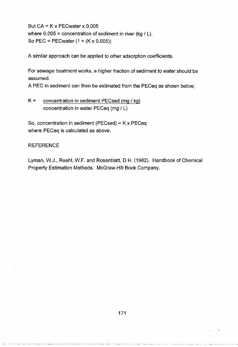
But CA = K X PECwater X 0.005 where 0.005 = concentration of sediment in river (kg / L).
So PEC = PECwater ( l + (K X 0.005))
A similar approach can be applied to other adsorption coefficients.
For sewage treatment works, a higher fraction of sediment to water should be assumed.
A PEC in sediment can then be estimated from the PECeq as shown below;
K = concentration in sediment PECsed (mg / kg2
concentration in water PECeq (mg / L)
So, concentration in sediment (PECsed) = K X PECeq
where PECeq is calculated as above.
REFERENCE
Lyman, W.J., Reehl, W.F. and Rosenblatt, D H. (1982). Handbook of Chemical Property Estimation Methods. McGraw-Hill Book Company.

ANNEX 7. Bioconcentration in fish
This seclion describes how a typical concentration in fish can be estimated using the
bioconcentration factor (BCF). Once an estimated concentration in fish is obtained,
this can be used along with dietary intake figures for humans and fish-eating
mammals or birds in order to estimate a daily intake (dose) of the substance by fish
consumption.
If the bioconcentration factor BCF is expressed on a lipid (fat) basis, this should be
converted to a fish whole body weight basis by assuming a standard fat content for
fish (e.g. 5% by weight), or an edible portion weight (relevant to human
consumption).
BCF whole body weight = conc. in fish (mglkg) l conc. in water (mglL)
Concn. in fish = conc. in lipid (mglkg) X 0.05
= BCF lipid X 0.05 conc. in water (mglL)
The concentration in fish can easily be calculated from the predicted environmental
concentration (PEC) in water,
Conc. in fish (mg 1 kg) = BCF whole body weight X PEC water
This calculation assumes the substance in water is all bio-available. This may not
be the case for the type of lipophilic (fat soluble) substance likely to bio-accumulate.
Thus the calculation is likely to give an overestimate of the actual fish concentration.

ANNEX 8. Dietary intake figures
In order to calculate a dose for higher animals from the predicted concentrations of a
substance in food (for instance fish, worms, plants etc.) knowledge of the daily
intake of such food by various species is required.
A8.1 Humans
Weekly human intake figures for a wide variety of foods are published annually by relevant bodies such as the Ministry of Agriculture Fisheries and Food in the UK. These figures can be used directly to estimate a human daily dose for the target food. The following is an example for fish.
Estimated fish consumption per person per week = 144 g
Estimated fish consumption per person per day = 20.6 g
Assuming that the fish contains a concentration of a substance of Y mg 1 kg (as estimated in Annex 7), the average daily dose of substance by a 60 kg person can
be estimated as,
Daily dose = Y X 0.0206 mgfkg body weight X 60
A similar approach can be carried out for other items of human food. Further methodology can be found in the Netherlands Government Report, "A Short-hand
Method: Predicting the Indirect Exposure of Man"
88.2 Animals
Daily dietary intake figures and conversion factors to allow a daily dose of a substance (mgfkg body weight) to be estimated have been published for several animal species and are summarized in the table below. These figures are from
"Appraisal of the Safety of Chemicals in Food, Drugs and Cosmetics, (1959), The Association of Food and Drug Officials of the United States".
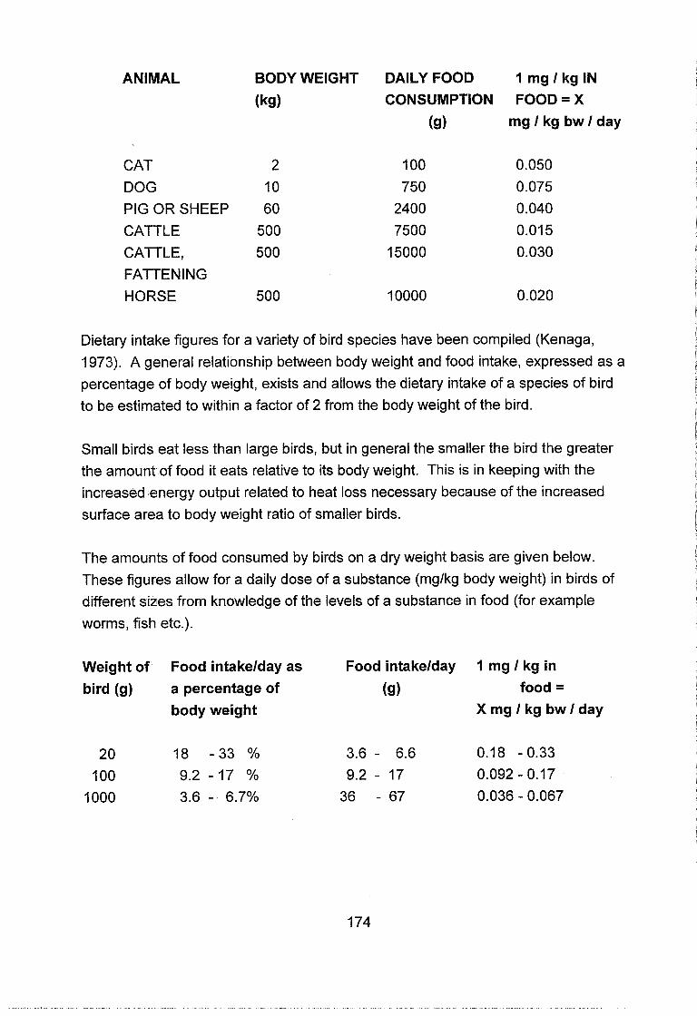
ANIMAL BODY WEIGHT DAILY FOOD 1 mg I kg IN
(kg) CONSUMPTION FOOD = X
(9) mg l kg bw l day
CAT 2 DOG I 0
PIG OR SHEEP 60
CATTLE 500
CATTLE, 500
FATTENING
HORSE 500
Dietary intake figures for a variety of bird species have been compiled (Kenaga,
1973). A general relationship between body weight and food intake, expressed as a
percentage of body weight, exists and allows the dietary intake of a species of bird
to be estimated to within a factor of 2 from the body weight of the bird.
Small birds eat less than large birds, but in general the smaller the bird the greater
the amount of food it eats relative to its body weight. This is in keeping with the
increased energy output related to heat loss necessary because of the increased
surface area to body weight ratio of smaller birds.
The amounts of food consumed by birds on a dry weight basis are given below.
These figures allow for a daily dose of a substance (mglkg body weight) in birds of
different sizes from knowledge of the levels of a substance in food (for example
worms, fish etc.).
Weight of Food intakelday as Food intakelday 1 mg l kg in
bird (g) a percentage of (9) food = body weight X m g l k g bwlday

A8.3 REFERENCES
The Association of Food and Drug Officials of the United States (1959). Appraisal of
the Safety of Chemicals in Food, Drugs and Cosmetics.
Ministry of Agriculture Fisheries and Food (1 991). Household Food Consumption and Expenditure 1990. Annual Report of the National Food Survey Committee. HMSO, London.
Kenaga, E. (1 973). Factors to be considered in the evaluation of the toxicity of
pesticides to birds in their environment. Environmental Quality and Safety II, pp 166-1 81. Academic Press, New York.


UNEPIIPCS Training Module No. 3
Section C
Risk Assessment
UNEPllPCS TRAINING MODULE SECTION C
ECOLOGICAL RlSK ASSESSMENT
TABLE OF CONTENTS
......................................................................... EDUCATIONAL OBJECTIVES 179 1 INTRODUCTION .......................................................................................... 179
........................................................... 2 ECOLOGY AND ECOTOXICOLOGY 181
2.1 Understanding how ecosystems work ............................................ 181 2.2 Human effects on ecosystems ......................................................... 194
2.3 Measurement of toxic effects on organisms and ecosystems ........ 198 2.4 Conclusion ...................................................................................... 201
3 THE BASIS OF ECOLOGICAL RISK ASSESSMENT .................................. 206 4 ECOLOGICAL RISK ASSESSMENT .......................................................... 207
4.1 An ecological risk assessment framework ...................................... 207 4.1.1 Problem formulation ......................................................... 2 0 7 4.1.2 Analysis of the situation .................................................... 212
4.1.2.1 Exposure Analysis .............................................. 212 4.1.2.2 Characterization of ecological effects ................. 213
4.1.2.3 Ecological response analyses ............................ 214
4.1.2.4 Stressor-response profile ................................... 216 4.1 .2.5 Data acquisition, verification, and monitoring ..... 216
5 ECOLOGICAL RISK CHARACTERIZATION ................................................ 217 ...................................................................................... 5.1 Integration -217
5.2 Risk description .............................................................................. 218 ........................................ 5.3 Interpretation of ecological significance 2 1 9
............... 5.4 Discussion between the risk assessor and risk manager 219 ................................. 5.5 Data acquisition, verification, and monitoring 219
5 BIBLIOGRAPHY ........................................................................................... 220 6 SELF ASSESSMENT EXERCISES .............................................................. 221

UNEPllPCS TRAINING MODULE
SECTION C
Ecological Risk Assessment
EDUCATIONAL OBJECTIVES
You should understand the fundamental requirements of a natural ecosystem in
terms of primary and secondary production and the various levels at which an
ecosystem may be affected. You should be familiar with the concepts of food
chains and webs and of bio-accumulation, bioconcentration and biomagnification. You should know the main habitat types, how ecosystems may be quantified and what factors, including potential toxicants, may affect their dynamic stability. From
the preceding knowledge, you should understand approaches to ecotoxicity testing and ecological monitoring. You should understand the essential concepts of ecological risk assessment and how it is carried out from problem formulation to risk
characterization. You should know how ecological systems may respond to stressors, the problems of exposure measurement, and the difference between assessmenf and measurement endpoints. You should understand how to analyse ecological risk and how to report your assessmenf to risk managers.
1 INTRODUCTION
This section is based partly on the USEPA document "A Framework for Ecological Risk Assessment" which describes the basics of ecological risk assessment. Two
other useful reviews of ecological risk assessment are "Ecological Risk Estimation"
by Bartell et al. (1992) describing an integrated approach to the assessment of aquatic ecological systems with an emphasis on simulation modelling and
"Ecological Risk Assessment" by Suter (1 993) which is an overview with excellent
sections on the application of population biology and ecology to risk assessment.

It is important to make clear the relationship between ecology, ecotoxicology and the
relevant aspects of risk assessment. Ecology and ecotoxicology are sciences
devoted to defining the relationship between chemical exposures and resultant
adverse-effects on ecosystems and their component organisms. Risk assessment is
a management tool used for making decisions, often with a great deal of uncertainty.
While the conclusions from ecology and ecotoxicology should be objectively
reached, societal perceptions and values often set the criteria applied in risk
assessment.

2 ECOLOGY AND ECOTOXlCOLOGY
Toxicology is most commonly concerned with effects of toxicants on humans.
Ecotoxicology is concerned with effects on organisms other than man. This has
three dimensions: toxicity to single species other than man, toxic effects on
interrelationships between species, and accumulation of toxicants by organisms and
their movement between organisms and species.
Study of ecotoxicology requires basic knowledge of ecology before the toxic effects
can be fully understood. Following an introduction to ecology and to the unifying
concept of a balanced ecosystem, this chapter examines in general terms the
effects of man on ecosystems and the methods for monitoring ecological effects.
To understand ecotoxicology requires knowledge of how organisms interact in
nature with each other (the biotic environment) and with the physical and chemical
aspects of the environment (the abiotic environment). This is the science of ecology
that can be viewed at several levels of organisation, at each of which there can be
toxic effects. Examples of these levels in ascending order of complexity are shown
in Table 1.
The following account of ecology illustrates how these and other toxic effects can
occur and assumes no previous knowledge of biology. It starts from a broad
consideration of the sustainability of ecosystems and is based on the review by
Wilkinson (1 996).
2.1 Understandina how ecosvsterns work
We can start from the simple assumption that there are two requirements that
organisms have from the environment to sustain their life which take precedence
over all other requirements:
(i) a supply of carbon to form the organic molecules of which organisms are
composed;
(ii) a supply of energy to power the chemical reactions that keep the organisms
alive.

Carbon is freely available in the environment as carbon dioxide in the air and as
various inorganic forms, including bicarbonate, dissolved in water. However,
organisms require organic carbon. Organisms can be divided into two major groups
. . depending upon how they obtain organic carbon, as shown in Table 2. Autotrophs
are organisms that can make all their chemical constituents from simple inorganic
compounds, making their carbon compounds from carbon dioxide. Heterotrophs are organisms that require to obtain complex organic molecules in their diet as they
are unable to synthesize them from simple carbon compounds like carbon dioxide.
In terms of number of species, autotrophs are very much in the minority, but they are
of absolutely crucial importance because they make the organic matter that all
organisms need. By far the biggest group of autotrophs, responsible for most of the
fixation of inorganic carbon into organic form on the earth, are the plants using the
process of photosynthesis, summarised as follows:
6C02 + 6H20 + light energy ---> C6H,,06 + 60,
This equation summarizes many reaction steps but illustrates the basic principle.
The other fundamental process, respiration, is a series of breakdown reactions
which, unlike photosynthesis, are undertaken by all organisms:
C6H1206 + 60, ---> 6C02 + 6H,O + chemical energy available for use in the cell
The living cell couples catabolic (breakdown) and anabolic (synthetic) reactions
using energy from breakdown processes to drive synthetic reactions.
Only autotrophs make new organic matter while all organisms consume it. Hence
growth of new body matter of autotrophs is called primary production. Production
of new body matter by heterotrophs that simply recycle already existing organic
matter is called secondary production. Therefore the production by the autotrophs
must be sufficient to meet the needs of both autotrophs and heterotrophs for
respiration. Hence in a balanced system there is a balance between production and
respiration. The photosynthesis by plants is balanced approximately by the total
community respiration.
Energy and carbon alone are not enough for life. About 20 different inorganic
nutrient ions are needed because of their roles in biochemical reactions in living
cells or because they are components of particular organic compounds e.g. nitrogen

in proteins. Plants absorb these from water and soil and they are passed to
heterotrophs in the diet.

Table 1. Levels of consideration in ecology
Level of organisation Description of level
1. Individual organism
or species
2. Population
3. Community
4. Ecosystem
Concerned with how physical
and chemical environmental
factors control which species
can occur in which place.
A group of individuals of a
single species living together
and having interrelationships
through gene exchange by
sexual reproduction.
A collection of populations of
different species living
together in one place (habitat)
giving species assemblages
characteristic of particular
conditions e.g. oak woodlands.
Organisms in a particular
habitat considered together
with their physical and
chemical environment, and
the processes linking the
organisms and environment
such as energy and nutrient
flow and biogeochemical
cycles. Ecosystems are
characterised by a degree of
sustainability.
Examples of toxicant effects
Alteration of the physical
and chemical factors can
affect the growth or survival
of particular species.
Effects on population size;
adaptation to toxicants by
tolerant mutants spreading
through population.
Changes in species
composition owing to
selectively different effects
of toxicants on different
species.
Interference with nutrient
recycling; concentration and
accumulation of toxic
substances in food chains;
alteration of productivity;
sustainability can be
impaired by these
alterations.
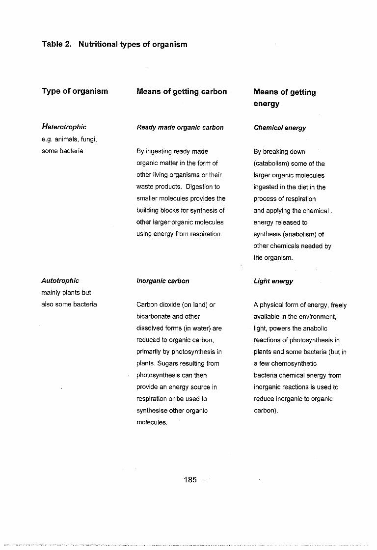
Table 2. Nutritional types of organism
Type of organism Means of getting carbon
ffeterotrophic
e.g. animals, fungi,
some bacteria
Autotrophic
mainly plants but
also some bacteria
Ready made organic carbon
By ingesting ready made
organic matter in the form of
other living organisms or their
waste products. Digestion to
smaller molecules provides the
building blocks for synthesis of
other larger organic molecules
using energy from respiration.
Inorganic carbon
Carbon dioxide (on land) or
bicarbonate and other
dissolved forms (in water) are
reduced to organic carbon,
primarily by photosynthesis in
plants. Sugars resulting from
photosynthesis can then
provide an energy source in
respiration or be used to
synthesise other organic
molecules.
Means of getting energy
Chemical energy
By breaking down
(catabolism) some of the
larger organic molecules
ingested in the diet in the
process of respiration
and applying the chemical
energy released to
synthesis (anabolism) of
other chemicals needed by
the organism.
Light energy
A physical form of energy, freely
available in the environment,
light, powers the anabolic
reactions of photosynthesis in
plants and some bacteria (but in
a few chemosynthetic
bacteria chemical energy from
inorganic reactions is used to
reduce inorganic to organic
carbon).

Some nutrients, e.g. nitrogen and phosphorus, may often be in low concentrations in
the environment compared with the amounts needed and so may limit plant growth
and primary production. Other nutrients such as various metal ions may be even
less abundant but are needed in such smaller amounts. Some trace elements, e.g.
copper, may be toxic when available in more than trace quantities but bio-availability
in soil or water may be regulated by natural binding agents reducing their effective
toxicity.
Organisms can be placed in a chain of dependence, known as a food chain, with
several different trophic levels (levels at which organisms feed) with plants or
primary producers absorbing light, inorganic carbon and nutrients, and passing
nutrients and organic molecules with their chemical energy to the higher trophic
levels of herbivores and carnivores (Fig. Eco-l).
Each trophic level produces waste material (as excretory products and dead matter)
and carbon dioxide from respiration. The waste products are broken down by
decomposer organisms (bacteria and fungi) which release nutrients back to the
environment where they are available for re-use. Thus nutrients cycle between
organisms and the environment. This is part of a more complex cyclic system - the
biogeochemical cycle. For each element utilised by organisms there is such a
cycle. The precise details differ between elements depending on the amount of the
element available, the uses to which organisms put it, where they store it in their
bodies, and the sinks for it in the environment.
All biogeochemical cycles incorporate the idea that, for any essential element at any
one time, part of the total naturally occurring amount of the element is in organisms
and part is in different components of the natural environment. Individual atoms or
molecules move between these compartments but the proportions in the different compartments remain roughly constant. These cycles must continue to function to
ensure a supply of nutrients for organisms and to ensure continuing biological
productivity.
Some organisms accumulate certain elements and compounds from the
environment (bio-accumulation) causing them to have very high body loads
relative to the outside concentrations (bioconcentration), e.g. organochlorines in
plant and animal tissues. If the accumulated substance is conserved (not broken
down by cellular processes) and stored, then a high dose will be given to the
organisms that eat the bio-accumulator.

CARNIVORES DECOMPOSERS
I I I
I l I l I I I I
primary producers) I
Carbon dioxide
Figure Eco. 1 Diagrammatic representation of a food chain. Arrows represent cycling of and pathways for energy, carbon and nutrients (carbon dioxide cycling has been omitted for clarity). The dotted line shows the route for input of energy from organic carbon and nutrients from detritus imported from another ecosystem. Organisms are in boxes and environmental requirements in ovals.

Because of losses of organic matter owing to respiration, each successive trophic
level often has a lower area biomass (mass of living material in a given area at one
time) or productivity than the levels below it. The body concentration of conserved
substances passed up the food chain can therefore increase up the chain
(biomagnification), sometimes resulting in toxic doses to organisms near the top of
the chain.
Nutrients and carbon are recycled. The only requirement for life not recycled directly
is light energy. Energy is lost to the environment by organisms. Consequently,
primary productivity is dependent on the continuous input of energy from the sun.
Primary productivity is also controlled by the availability of all the other requirements
for plant growth, carbon dioxide, water and nutrients. Since the availability of all
these substances differs between habitats, different levels of primary production are
characteristic of different places (Table 3).
The rate of secondary production depends on the availability of energy, carbon, and
nutrients from the primary producers. Thus, factors affecting plant growth usually
affect total production of the whole system.
An exception to immediate dependence on plant growth is seen in detritus-based
systems such as estuaries. In estuaries the hydrographic conditions cause
suspended particles from land drainage, the sea and freshwater to accumulate,
giving turbid water which restricts light penetration for photosynthesis. The
accumulated suspended matter includes much organic detritus that is instead used
as a carbon, energy and nutrient source by estuarine heterotrophs. There is so
much detritus that there is high secondary production despite restricted
photosynthesis in this system. The primary production has been done in other
habitats from which the detritus has been transferred
A food web is a more realistic concept than a food chain. Fig. 2 presents a very
simple food web based on imaginary species (most natural ones would contain
many more species). Even with such a simple one there can be a complex pattern
of flow of energy, carbon and nutrients, based on the feeding preferences of
different species, as indicated by the lines on the diagram. For any particular habitat
there is a degree of stability by which the same assemblages of species are present
in a food web in successive years, with the same dominant and rare species, with
the same flow pathways important and others less so.

to^ carnivores P
2nd carnivores
\ 1st carni
herbivores
primary producers Figure Eco.2 Theoretical food web for a group of imaginary species, indicated by letters (After W~lkinson, 1996). Lines joining the imaginary species indicate feeding relationships and hence pathways for the flow of energy, carbon and nutrients. Note the complexity of the diagram since species have feeding preferences. Some species feed at more than one trophic level.

Organisms do not occur together wholly by chance. A particular habitat has its own
set of environmental conditions to which an organism must be tolerant if it is to survive. Different species have different tolerances to physical and chemical
environmental factors (abiotic factors) e.g. temperature, rainfall, soil nutrient status. The range of abiotic factors tolerated along a gradient of such factors (Fig. 3) can be considered as the "theoretical niche" of the species. In practice, species usually occupy a narrower range of conditions than this - the "realised niche". They do not occur at the extremities of the theoretical range because of interactions there with other organisms (biotic interactions). For example a species will be best adapted to
the environment near to the middle of its tolerance range. Towards the extremities it might be under some stress. It will not compete there with other better-adapted
species, which are towards the middle of their tolerance ranges.
This leads us to the concept of an ecosystem. An ecosystem consists of all the organisms in a particular place or habitat, their interrelationships with each other in terms of nutrient, carbon and energy flows, and in terms of biotic determinants of community composition such as competition between species, the physical habitat
and the abiotic factors associated with it, which also play a role in determining community composition and in determining primary, and hence secondary
production
Ecosystems can be quantified, for example, in terms of the fluxes of carbon, energy and nutrients and the productivity of each trophic level. They can be quantitatively modelled using computers to enable predictions to be made about ecosystem performance.

Table 3. Generalized productivity of different habitat types (after Odum, 1985)
Habitat type
Deserts
Grasslands, deep lakes, mountain forests,
some agriculture
Moist forests and secondary communities,
shallow lakes, moist grasslands, most
agriculture
Some estuaries, springs, coral reefs,
terrestrial communities on alluvial plains,
intensive year-round agriculture
Continental shelf waters
Deep oceans
Gross productivity (grams of dry matter per square metre per day) indicative of primary productivity
less than 0.5
0.5 - 3.0
less than 0.5


Probably the most important characteristic of ecosystems is their dynamic stability. They remain broadly constant over time in species composition and abundance and
in the magnitudes of processes despite environmental variations. Although the
climate fluctuates from year to year, the structure of the ecosystem tends to be
stable within limits, and therefore it is sustainable.
An example of dynamic stability is in population sizes. Man's population does not
fluctuate wildly from year to year because the generation time is about 20 years and
several generations are overlapping. A contrast is in many insects where
reproduction occurs every year and the life span is only one year or less. There can
be fluctuations of several orders of magnitude in population size over several years
but they fluctuate around a mean value. This may result from density-dependent
factors, environmental factors whose intensity or effect depends on the population
density. For example, at high density, food may be short giving a population crash, while at low density, the abundance of food may allow population size to increase,
thus fluctuating over several years about a mean.
Ecosystem stability is not rigid. Some systems change naturally - hence the
dynamic nature of the stability. On a short time scale this happens with winter and
summer aspects of a community in a temperate climate. On a longer time scale
there is ecological succession where one community naturally replaces another on
an area of land or water, usually as a result of the modification of the habitat
conditions by the organisms that are replaced so that it is no longer suitable for their
own survival. This happens particularly where an open area of land or water is
available for colonisation.
An example of ecological succession is the formation and growth of maritime sand
dune systems. Near the high tide mark on a beach is an inhospitable environment
for plants, windswept with high water loss by evaporation and with sand abrasion,
high sand surface temperatures in summer, and a low nutrient and highly saline soil,
subject to erosion by waves and wind. Only a few species, the dune-building
grasses, can tolerate this environment, forming an open community where,
unusually, most ground area is not colonised. These grasses grow best through
depositing sand that they stabilise, so building up dunes. The dune soil becomes
less saline due to leaching by rainwater, nutrients accumulate from the grass litter
aided by nitrogen-fixing bacteria associated with their roots, and the growing dunes
provide shelter. Going inland the habitat becomes progressively more normal, less
inhospitable, and there is a progressive replacement of the dune building grasses by

a wider range of more normal, less tolerant plants. Ultimately a closed (complete ground coverage) climax community is achieved in equilibrium with the climate and
with any local conditions such as soil type.
Mature stable ecosystems are characterised by a preponderance of organisms referred to as K-strategists, species which succeed by being well adapted to their environment. Earlier stages in a succession may have a greater proportion of
r-strategists, organisms with wide environmental tolerance which do not survive so well in stable habitats in competition with more precisely adapted K-species. By contrast r-strategists are highly reproductive, flooding the environment with their
propagules, ready to colonize opportunistically any habitat space which may become available. In stressful environments, either man-made stress or naturally
harsh conditions, tolerance to abiotic factors becomes a greater determinant of
community composition than biotic interactions, and r-strategists predominate.
The above description of the ecosystem concept stresses the ability of such systems to remain stable within limits in various ways. Maintenance of this stability is the key to understanding ecotoxicology and the effects on ecosystems caused by pollutants.
2.2 Human effects on ecosystems
Human beings affect the dynamic balance of ecosystems in two ways, by pollution and by physical disturbance. Here we are concerned with toxic effects and so will only consider pollutants. Pollutants are substances which potentially can have an impact on ecosystems either because they are novel chemicals synthesised by man
which normal decomposer organisms are not accustomed to dealing with, or because they are discharged in unusually high amounts andlor to a system from which they did not come e.g. human waste from food grown on land discharged in
concentrated form through sewer outlets to rivers or the sea.
Ecosystems become unbalanced through pollutant (toxicant) effects. The stability is disturbed and the productivity and recycling reduced meaning that they are no longer sustainable systems. This results from the selective action of toxicants, affecting different species in different ways, or to different extents, or at different concentrations. There may be lethal effects where species are killed but more commonly there are sublethal effects where species remain alive but with reduced growth or reduced reproductive ability or modified development, all leading to ecosystem alteration. A summary of ways in which toxic pollutants may affect

organisms at the different levels of consideration in ecology is given as a flow
diagram in Fig. Eco.4.
At an ecosystem level the above effects can give rise to various symptoms of stress
in the system. However stress can be due not only to toxicants but also to non-toxic
pollutants, to physical disturbance, and to natural stress in extreme habitats. Part of the art of measuring biological effects of pollution (summarised later) is in
distinguishing man-made from natural stress effects. The symptoms of stress in
ecosystems are given below in Table 4.
As mentioned above, not all pollutants are directly toxic. Nonetheless some of the
non-toxic ones are relevant to this account because they can have a secondarily
toxic effect. An example is enrichment of a water body with plant nutrients such as
nitrogen and phosphorus (eutrophication) which can enter as pollutants from
sewage, fertiliser run-off or some industry.
Assuming adequate supplies of carbon and light, plant growth will be limited by
nutrients. Nutrient pollution can have a fertilising rather than a toxic effect.
Considerable enrichment can give massive unchecked growth of plants which
outstrips the ability of herbivores to graze on it. The decay of the excess plant
biomass by bacterial activity then creates a demand for oxygen for bacterial
respiration that may exceed its rate of supply from the overlying atmosphere. The resulting de-oxygenation of water can have a lethal effect on aquatic animals since
most animals require respiratory oxygen more than plants which can produce their
own oxygen by photosynthesis. Some of these effects on ecosystems can be used
in biological measurement of pollution. The next section gives an overview of such
techniques.

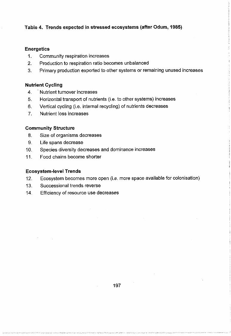
Table 4. Trends expected in stressed ecosystems (after Odum, 1985)
Energetics I. Community respiration increases
2. Production to respiration ratio becomes unbalanced
3. Primary production exported to other systems or remaining unused increases
Nutrient Cycling 4. - Nutrient turnover increases
5. Horizontal transport of nutrients (i.e. to other systems) increases
6. Vertical cycling (i.e. internal recycling) of nutrients decreases
7. Nutrient loss increases
Community Structure 8. Size of organisms decreases 9. Life spans decrease
10. Species diversity decreases and dominance increases
1 1. Food chains become shorter
Ecosystem-level Trends 12. Ecosystem becomes more open (i.e. more space available for colonisation)
13. Successional trends reverse 14. Efficiency of resource use decreases
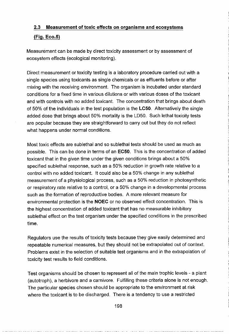
2.3 Measurement of toxic effects on organisms and ecosystems
(Fig. Eco.5)
Measurement can be made by direct toxicity assessment or by assessment of
ecosystem effects (ecological monitoring).
Direct measurement or toxicity testing is a laboratory procedure carried out with a single species using toxicants as single chemicals or as effluents before or after
mixing with the receiving environment. The organism is incubated under standard conditions for a fixed time in various dilutions or with various doses of the toxicant
and with controls with no added toxicant. The concentration that brings about death
of 50% of the individuals in the test population is the LC50. Alternatively the single added dose that brings about 50% mortality is the LD50. Such lethal toxicity tests
are popular because they are straightforward to carry out but they do not reflect what happens under normal conditions.
Most toxic effects are sublethal and so sublethal tests should be used as much as
possible. This can be done in terms of an EC50. This is the concentration of added toxicant that in the given time under the given conditions brings about a 50%
specified sublethal response, such as a 50% reduction in growth rate relative to a control with no added toxicant. It could also be a 50% change in any sublethal measurement of a physiological process, such as a 50% reduction in photosynthetic
or respiratory rate relative to a control, or a 50% change in a developmental process such as the formation of reproductive bodies. A more relevant measure for environmental protection is the NOEC or no observed effect concentration. This is
the highest concentration of added toxicant that has no measurable inhibitory sublethal effect on the test organism under the specified conditions in the prescribed
time.
Regulators use the results of toxicity tests because they give easily determined and repeatable numerical measures, but they should not be extrapolated out of context.
Problems exist in the selection of suitable test organisms and in the extrapolation of toxicity test results to field conditions.
Test organisms should be chosen to represent all of the main trophic levels - a plant (autotroph), a herbivore and a carnivore. Fulfilling these criteria alone is not enough. The particular species chosen should be appropriate to the environment at risk where the toxicant is to be discharged. There is a tendency to use a restricted

V); 0 .= *- F CO
3 CC-
CC- *

range of species strains that can be found in culture collections. These strains may have evolved over long periods of repeated subculturing so as to have different
responses from the original organisms isolated. An extreme example of an inappropriate choice that has occurred was the use of the marine oyster embryo bioassay to test a substance to be discharged to a freshwater river.
Otherwise ecologically inappropriate tests may have their uses as a standard
reference tests to rank the general toxicity of many different chemicals. This may
permit the choice of the least toxic substance for given process.
What cannot be done easily from laboratory tests is prediction of effects on the
structure or functioning of ecosystems. It is inherent in the nature of a toxicity test that it is done under constant laboratory conditions that cannot mimic the complex
and fluctuating field environment and the biotic interactions that occur.
One approach being taken to remedy the lack of relevance of laboratory tests to real ecosystems is the development of tests that are carried out in the field. The
organism is grown captive in a polluted location and some measure of its growth, physiology, biochemistry or survival is compared to similarly treated captive organisms in a similar but less polluted control environment. These methods are in their infancy and do not always find favour because of the undefined nature of the conditions and uncertainty that the control environment is similar to the test
environment in all features except the pollution.
Recently the British water industry has started to build toxicity criteria into consents given to discharge liquid effluents into watercourses or coastal waters. Previously the consents contained only physical and chemical limits on effluent composition. The addition of toxicity criteria makes them more effective for complex effluents where there might be synergistic effects between components or where there might be so many components that they were not all regulated in the consent. It is the
total toxicity of the effluent that is assessed rather than its composition of specific chemicals.
Enforcement of toxicity criteria in consents to discharge could be a problem. While toxicity tests are attractive to some because of their ease and simplicity, routine application of tests on a wide range of organisms with a large number of effluents could be very costly, especially if vertebrates such as fish are used, since they require expensive facilities and government approval. An alternative quick

screening technique has been devised based on bacterial luminescence, of which
Microtox is one proprietary test. This is based on light emission by a culture of
luminescent bacteria. When the bacteria are in toxic solutions, their light emission is
reduced relative to identical uncontaminated solutions. Hence an EC50 can be
calculated in terms of a 50% reduction in luminescence relative to the control. This
might be thought to be an example of an inappropriate test organism but it is used
as a screening test. If serious toxicity is shown in the relatively quick and cheap
Microtox test then more relevant but time consuming and expensive tests with the
full range of organisms can be carried out.
Ecological monitoring is a broader assessment of the ecological effects of toxicants
than is given by toxicity testing. It is defined as the assessment of effects of
toxicants and pollutants in an ecological context, either by means of their
accumulation in organisms other than man, or by looking for abnormal ecological effects at the level of species, community or ecosystem. It performs a different role
from that of chemical analysis of toxicants in the environment. Chemical analysis
usually relies on occasional instantaneous sampling. It does not necessarily
indicate average, maximum or minimum environmental values of the toxicant.
Ecological monitoring avoids the very frequent chemical sampling necessary to get
over this problem. Indigenous organisms integrate concentrations of toxicant over
time. Furthermore they show what chemical sampling cannot do - the effects of the
toxicants on natural communities. Ecological methods do not give numerical
estimates of toxicant concentrations, so both chemical and ecological approaches
are necessary.
Ecological monitoring can use naturally occurring organisms in the field or
organisms transplanted to the field for the purpose, and may be supported by
laboratory tests. Table 5 presents an illustrative selection of approaches to
ecological monitoring, with a bias towards aquatic assessment where these
approaches have been most highly developed.
2.4 Conclusion
Toxicants can disturb the sustainability of natural ecosystems by a variety of effects
on species, populations, communities and ecosystem processes. Hoxever, such
systems have some capacity to absorb potentially toxic substances because of their "dynamic stability". Toxicity testing has limitations in predicting ecological effects
and chemical measurement of environmental toxicants must be accompanied by

ecological monitoring. Specialist knowledge is needed to distinguish between
ecological effects due to the effects of pollution and those due to naturally-occurring
environmental conditions that impose severe stress.

Table 5. An overview of selected measures used in ecological monitoring
l Assessments carried out in the field
Using organisms Pollutant Some organisms accumulate metals,
occurring accumulation by radionuclides and some hydrocarbons to
naturally in the organisms high levels in their tissues in proportion to
environment (bio-accumulation the external concentration. Gives higher
monitoring) more detectable concentrations. Integrates
concentration through time. May indicate
biologically active fractions of the substance.
Algae may indicate dissolved fraction while
animals feeding on suspended matter (e.g.
mussels) may indicate particulate fraction.
Assessments using Presence or absence of indicator organisms
single species There are few genuine indicators solely by
presence so must be used with care.
Biochemical measurements on single
species - measurement of activity or amount
of substances induced by presence of
pollutants e.g. enzymes or metal-binding
proteins.
Pathology - presence of tumours induced by
pollutants
Assessments using Age structure - in a species that can be
communities and aged and which recruits annually, abnormal
populations age structure may indicate a failure to recruit
in one year due to pollution or to natural
climatic factors.
Life-forms and successions - successions
regressed to earlier stages with abnormal
abundance of opportunists may indicate
stress.

Table 5 (continued) 1. Assessments carried out in the field
Numerical structure
(i) Species richness - fewer species may
occur under stress
(ii) Diversity - there are many numerical
indices which are mathematical formulations
of species number, numbers of individuals,
and the distribution of individual numbers
between species. Used as general
assessments of community structure in
ecology but variations from expected values
can indicate toxicant induced stress. Also
specially developed indices such as the
Trent Biotic Index which indicates degree of
sewage stress on animal communities in
rivers based on numbers of taxa and
presence of key species or groups
Using organisms
planted out at test
site
In-situ toxicity assessment using
measurements of the growth of organisms at
a test site compared with a control site.
Colonisation of artificial substrata - provides
a uniform substratum that can be compared
between different sites using numerical
indices (see above) of the communities of
small organisms that develop.
Colonisation of cleared natural substrata - again using numerical indices of community
structure may also show whether an
alternative community can develop under
pollutant influence when the established one
is dislodged.
Bio-accumulation monitoring using monitors
artificially placed at a variety of test sites to
permit comparison.

3. Laboratory-to-field extrapolation - relationship of the estimate of toxicity
gathered in the laboratory to the effects expected in the field situation. Laboratory situations are kept simple compared to the reality of the field and are designed to rank toxicity rather than to mimic the field situation. Laboratory tests strictly control the route of exposure and limit the behaviour
of organisms. In the field there are no such restrictions.
4. Field to field (or habitat to habitat) extrapolation - relationship of one field or habitat to another. It is most unlikely that any two habitats can be identical. Streams on one side of a continental divide tend to have flora and fauna that
are different from those in comparable streams on the other side. Even controlled field studies are difficult to replicate. The qualitative effect of a toxicant may be the same but the quantitative relationship may be very
different.
5. Indirect effects - the toxicant effects due to the disruption of the ecosystem in addition to direct impacts on ecosystem components. The elimination of photosynthetic organisms in a pond by a herbicide will eventually eliminate invertebrate herbivores and the fish that rely upon them as a food source.
6. Organizational levels - the transmission of effects up and down levels of biological organization. A decline in reproductive success at the individual organism level may decrease the rate of growth of a population. Conversely,
a toxicant which causes the decrease in a herbivore (plant eating) population, eliminating much of the top-down control at community level, will allow plant populations to increase even if the toxicant reduces the maximum rate of plant growth.
7. Spatial and temporal scales - exist in a variety of dimensions relating to the life span and size of the organisms and systems under investigation. One
3 day and 10 m may represent several generations and the entire world of many micro-organisms, but have no relevance to a Californian redwood tree.
Heterogeneity of both of these variables contributes to the diversity of species and genotypes.
8. Recovery - the rate at which a system can be restored to its original state. If recovery does occur, it generally depends upon the ability of colonizing organisms to become established upon the impacted site and therefore the

isolation of the damaged ecosystem is important. Initial conditions are extremely important since several new steady states can be reached from similar initial conditions. Recovery to the initial state may be improbable and
a-more realistic goal may be a new steady state appropriate to the factors selected as assessment endpoints.
4.1.2.4 Stressor-response profile
The stressor-response profile is analogous to a dose-response curve in that it
corresponds to a single species toxicity test expanded to the community and ecosystem level. It is important to define the uncertainties, qualifications, and
assumptions made at each step.
One of the difficulties in the quantification of the stressor-response profile is that
many of the extrapolations are essentially qualitative. Phylogenetic extrapolations
are rarely quantified.
Laboratory organisms are generally healthy and laboratory conditions do not mimic
availability of micronutrients, behavioural opportunities, and other factors important
in an ecosystem. Field studies include many climatalogical and structural stressors that are independent of the introduced stressor. In addition, there is unlikely to be
an ecosystem within range of a laboratory that has not been subjected to an anthropogenic stressor which may confound even the best designed study.
4.1.2.5 Data acauisition. verification. and monitorina
Basic research on the effects of stressors on ecosystems, improvement in test methods, knowledge of molecular mechanisms, and improvements in modelling provide critical input to this stage of risk assessment.

5 ECOLOGICAL RISK CHARACTERIZATION
Risk characterization is the final stage of the risk assessment process. This aspect
of a risk assessment is comprised of risk estimation and a risk description. The
overall process is a correlation of the ecological effect with the environmental
concentration to provide a likelihood of effects given the distribution of the stressor
within the system.
Assessing the probability of toxic impacts is analogous to the weather forecaster's
prediction of rain. If the forecaster says that today there is a 50% chance of rain in
the local area, this means that, given the conditions observed, the chance is that
rain will occur in 50 out of 100 observations. Similarly, ecotoxicology attempts to
make predictions regarding the risk (probability) of an effect of a given substance on
an ecosystem, given knowledge of its concentration and the nature of the
ecosystem. Because this is still a developing science, ecological predictions of this
kind may be less reliable than weather forecasts!
5.1 Integration
Relating exposure to toxicity is not easy. A fish LC,, value tells nothing about the
loss of nitrogen fixation from an ecosystem. The most widely used method of
estimating ecological risk is the quotient method, simply dividing the expected
environmental concentration by the hazard (compare Part B, "Environmental Risk
Assessment").
Risk quotient = Expected environmental concentration I Concentration producing an
unacceptable environmental effect
This is a qualitative expression of risk without regard to the probability distributions
of the chemical concentrations or the effects. Distributions of each can be plotted and the distribution of expected effects can be calculated.
The quality and source of the data used in risk assessment contributes to its
uncertainty. Toxicological data vary according to the strain or test organism used. Field studies are noted for the difficulty of interpretation. Many multispecies tests
and field studies are designed to look at only a few populations or other attributes of
the ecosystem. For example, a standardized aquatic microcosm may contain 16

species that are initially inoculated into the system. However, in reporting results for publication, the dynamics and interactions of all species are not reported because it
would be cumbersome and expensive. Only the dynamics of the organisms and interactions that are the apparently critical components are reported.
Anecdotal data from field or multispecies tests are also difficult to interpret. Omission or inclusion of information in a report may reflect more the nature of the
researcher than the presence or absence of an effect.
5.2 Risk description
There are two aspects to this - ecological risk summary and the interpretation of ecological significance.
The ecological risk summary summarizes the risk estimation results and its uncertainties. The crucial decision concerns the accuracy of the risk estimation. This
depends upon: Sufficiency of data
e Corroborative information
e Evidence of causality
Sufficiency of the data relates to the quality of the data and its completeness.
Corroborative information is data derived from similar studies with similar stressors
that tend to support the conclusions of the risk assessment. However, lack of similarity to previous conclusions or ecological theory does not mean that the current study is in error. It may mean that some fundamental assumption has to be re-
assessed.
Evidence of causality, if available, is the most important aspect of the data assessment process. However, correlational data may be all that are available for impacts at the level of interspecies interactions. Correlation does not denote cause
and effect. In a complex system, correlations due to chance may occur.
If additional data or reformulation of the conceptual model is required, the assessment process returns to data acquisition, verification, and monitoring, and a further attempt is made to obtain a usable and accurate risk assessment.

5.3 lnter~retation of ecoloaical sianificance
Finally, an interpretation of ecological significance is produced that details the expected size, variation in time and space, and probability of each significant effect. Judgment may have to be made about the recovery potential of the affected ecosystem. This requires a decision as to whether the ecosystem can regain the properties that are regarded as valuable. These properties will have been defined
by the assessment endpoints.
5.4 Discussion between the risk assessor and risk manager
The risk manager needs to know the range of impacts, uncertainties in the data, the probabilities of effects, and the stressor-response function. These factors can then be taken into account alongside social, economic and political realities and riswbenefit assessment in selecting management options.
5.5 Data acquisition, verification, and monitoring
The importance of the data acquisition, verification, and monitoring process in the
development of accurate risk assessments has been emphasized. Models, no matter how sophisticated, are simply attempts to understand processes and codify relationships. Only the reiteration of the predictive (risk assessment) and
experimental (data acquisition, verification, and monitoring) process can bring models close to being a true picture of reality.

5 BIBLIOGRAPHY
Anderson, J M ( l 981) Ecology for the Environmental Sciences: Biosphere,
Ecosystems and Man. London: Edward Amold Ltd.
Bartell, S M, Gardner, R H, and O'Neill, R V (1 992) Ecological Risk Estimation. Chelsea, MI: Lewis Publishers.
Beeby, A (1 993) Applying Ecology. London: Chapman and Hall.
Moriarty, F (1 988) Ecotoxicology. 2nd edn. London: Academic Press.
Odum, EP (1 985) Trends in stressed ecosystems, Bioscience, 35, 41 9-422.
Sheehan PJ, Miller DR, Butler GC and Bourdeau P (1984) Eflects of Pollutants at
the Ecosystem Level, SCOPE. Chichester: Wiley.
Suter (11), G W. (1 990) Environmental risk assessment/environmental hazard
assessment: similarities and differences. In Landis, W G and van der Schalie, W H, Aquatic Toxicology and Risk Assessment, 13th Volume, ASTM STP 1096, pp. 5-1 5. Philadelphia, PA: American Society for Testing and Materials.
Suter (II), G W (1 993) Ecological Risk Assessment. Chelsea, MI: Lewis Publishers.
Wilkinson, M (1 996) Ecotoxicity. In Fundamental Toxicology for Chemists, eds. J.H. Duffus and H.G.J. Worth. Cambridge: The Royal Society of Chemistry.
World Health Organization (1986). Environmental Toxicology and Ecotoxicology: Proceedings of the Third International Course, Environmental Health series No 10. Copenhagen: WHO Regional Office for Europe.

6 SELF ASSESSMENT EXERCISES
What are the two fundamental requirements for sustaining life? What are autotrophs, how do they obtain carbon, and how do they obtain
energy? What are heterotrophs, how do they obtain carbon, and how do they obtain energy? What are primary production and secondary production? What are the levels of consideration in ecology and what toxicant effects may be observed at these levels?
What is a typical food chain and what are the associated trophic levels? How does a food chain relate to a food web? What are bio-accumulation, bioconcentration and biomagnification?
What are the 6 main habitat types? What is a tolerance range and what defines it? What is an ecosystem and how may ecosystems be quantified?
What is dynamic stability in an ecosystem? What characterizes a mature stable ecosystem? What are pollutants and how can they unbalance ecosystems?
What trends are to be expected in stressed ecosystems? How can a nutrient indirectly cause toxicity in an ecosystem? What methods are available for toxicity testing of potential ecological toxicants? What approaches may be used in ecological monitoring for possible damage by pollutant substances? Define ecological risk assessment, stressor, hazard, and exposure? Briefly define problem formulation, hazard assessment, exposure assessment, and risk characterization? Stresses can be of what three categories? What five characteristics can stressors have that are derived in part from use patterns? What are some possible interactions between the stressor and the ecological
system? What is an assessment endpoint? What is a measurement endpoint? What factors make risk assessment a "scientific process"? What is the goal of the exposure analysis? How may exposure be measured? What is the most critical aspect of the risk assessment process?
27. What are the criteria used to judge the importance of data when
characterizing ecological effects?
28. Describe the eight possible relationships between assessment and
measurement endpoints.
29. What is one of the difficulties in evaluating the stressor-response relationship?
30. Describe risk characterization.
31. What is the quotient method of estimating risk? What is a weakness of this analysis.
32. List the three general aspects of the analysis for the ecological risk summary
and describe each. 33. What question should be borne in mind in the interpretation of ecological
significance of data?
34. List the most important factors in a report to the risk manager.