underwater depth imaging using time- correlated single ... · underwater depth imaging using...

Underwater depth imaging using time-correlated single-photon counting

Aurora Maccarone,1 Aongus McCarthy,1 Ximing Ren,1 Ryan E. Warburton,1 Andy M. Wallace,2 James Moffat,3 Yvan Petillot,2 and Gerald S. Buller1

1Institute of Photonics and Quantum Sciences, and Scottish Universities Physics Alliance (SUPA), Heriot-Watt University, Edinburgh, EH14 4AS, UK

2Institute of Sensors, Signals & Systems, School of Engineering and Physical Sciences, Heriot-Watt University, Edinburgh, EH14 4AS, UK

3Defence Science and Technology Laboratory, Portsdown West, PO17 6AD, UK

Abstract: A depth imaging system, based on the time-of-flight approach and the time-correlated single-photon counting (TCSPC) technique, was investigated for use in highly scattering underwater environments. The system comprised a pulsed supercontinuum laser source, a monostatic scanning transceiver, with a silicon single-photon avalanche diode (SPAD) used for detection of the returned optical signal. Depth images were acquired in the laboratory at stand-off distances of up to 8 attenuation lengths, using per-pixel acquisition times in the range 0.5 to 100 ms, at average optical powers in the range 0.8 nW to 950 μW. In parallel, a LiDAR model was developed and validated using experimental data. The model can be used to estimate the performance of the system under a variety of scattering conditions and system parameters.

©2015 Optical Society of America

OCIS codes: (110.6880) Three-dimensional image acquisition; (280.3640) Lidar; (030.5260) Photon counting; (110.0113) Imaging through turbid media; (010.4450) Oceanic optics.

References 1. S. Reed, Y. Petillot, and J. Bell, “An automatic approach to the detection and extraction of mine features in

sidescan sonar,” IEEE J. Oceanic Eng. 28(1), 90–105 (2003). 2. J. S. Jaffe, M. D. Ohman, and A. De Robertis, “OASIS in the sea: measurements of the acoustic reflectivity of

zooplankton with concurrent optical imaging,” Deep Sea Res. Part II Top. Stud. Oceanogr. 45(7), 1239–1253 (1998).

3. M. Evangelidis, L. Ma, and M. Soleimani, “High definition electrical capacitance tomography for pipeline inspection,” Prog. Em. Res. 141, 1–15 (2013).

4. A. Bellettini and M. A. Pinto, “Theoretical accuracy of synthetic aperture sonar micronavigation using a displaced phase-center antenna,” IEEE J. Oceanic Eng. 27(4), 780–789 (2002).

5. J. R. V. Zaneveld and W. Pegau, “Robust underwater visibility parameter,” Opt. Express 11(23), 2997–3009 (2003).

6. R. D. Richmond and S. C. Cain, Direct-Detection LADAR Systems (SPIE, 2010). 7. D. M. Kocak, F. R. Dalgleish, F. M. Caimi, and Y. Y. Schechner, “A focus on recent developments and trends

in underwater imaging,” Mar. Technol. Soc. J. 42(1), 52 (2008). 8. J. S. Jaffe, K. D. Moore, J. McLean, and M. P. Strand, “Underwater optical imaging: status and prospeccts,”

Oceanography (Wash. D.C.) 14(3), 64–75 (2001). 9. F. R. Dalgleish, F. M. Caimi, W. B. Britton, and C. F. Andren, “Improved LLS imaging performance in

scattering-dominant waters,” Proc. SPIE 7317, 73170E (2009). 10. W. Hou, Ocean Sensing and Monitoring (SPIE, 2013). 11. S. G. Narasimhan, S. K. Nayar, B. Sun, and S. Koppal, “Structured light in scattering media,” in Tenth IEEE

International Conference on Computer Vision (ICCV’05) (IEEE, 2005), pp. 7. 12. B. Cochenour, S. O’Connor, and L. Mullen, “Suppression of forward-scattered light using high-frequency

intensity modulation,” Opt. Eng. 53, 1–8 (2014). 13. J. Watson and O. Zielinski, Subsea Optics and Imaging (Woodhead Publishing Limited, 2013). 14. N. R. Gemmell, A. McCarthy, B. Liu, M. G. Tanner, S. D. Dorenbos, V. Zwiller, M. S. Patterson, G. S. Buller,

B. C. Wilson, and R. H. Hadfield, “Singlet oxygen luminescence detection with a fiber-coupled superconducting nanowire single-photon detector,” Opt. Express 21(4), 5005–5013 (2013).

15. H.-K. Lo, M. Curty, and K. Tamaki, “Secure quantum key distribution,” Nat. Photonics 8(8), 595–604 (2014).

#251754 Received 13 Oct 2015; revised 7 Dec 2015; accepted 8 Dec 2015; published 23 Dec 2015 © 2015 OSA 28 Dec 2015 | Vol. 23, No. 26 | DOI:10.1364/OE.23.033911 | OPTICS EXPRESS 33911

16. P. J. Clarke, R. J. Collins, V. Dunjko, E. Andersson, J. Jeffers, and G. S. Buller, “Experimental demonstration of quantum digital signatures using phase-encoded coherent states of light,” Nat. Commun. 3, 1174 (2012).

17. W. Becker, Advanced Time-Correlated Single Photon Counting Techniques (Springer, 2005). 18. G. S. Buller, R. D. Harkins, A. McCarthy, P. A. Hiskett, G. R. MacKinnon, G. R. Smith, R. Sung, A. M.

Wallace, R. A. Lamb, K. D. Ridley, and J. G. Rarity, “Multiple wavelength time-of-flight sensor based on time-correlated single-photon counting,” Rev. Sci. Instrum. 76(8), 083112 (2005).

19. G. S. Buller and A. M. Wallace, “Ranging and three-dimensional imaging using time-correlated single-photon counting and point-by-point acquisition,” IEEE J. Sel. Top. Quantum Electron. 13(4), 1006–1015 (2007).

20. A. McCarthy, X. Ren, A. Della Frera, N. R. Gemmell, N. J. Krichel, C. Scarcella, A. Ruggeri, A. Tosi, and G. S. Buller, “Kilometer-range depth imaging at 1,550 nm wavelength using an InGaAs/InP single-photon avalanche diode detector,” Opt. Express 21(19), 22098–22113 (2013).

21. A. McCarthy, R. J. Collins, N. J. Krichel, V. Fernández, A. M. Wallace, and G. S. Buller, “Long-range time-of-flight scanning sensor based on high-speed time-correlated single-photon counting,” Appl. Opt. 48(32), 6241–6251 (2009).

22. S. Pellegrini, G. S. Buller, J. M. Smith, A. M. Wallace, and S. Cova, “Laser-based distance measurements using picosecond resolution time-correlated single-photon counting,” Meas. Sci. Technol. 11(6), 712 (2000).

23. S. Q. Duntley, “Light in the sea,” J. Opt. Soc. Am. 53(2), 214–234 (1963). 24. R. C. Smith and K. S. Baker, “Optical properties of the clearest natural waters (200-800 nm),” Appl. Opt. 20(2),

177–184 (1981). 25. G. M. Hale and M. R. Querry, “Optical constants of water in the 200-nm to 200-µm wavelength region,” Appl.

Opt. 12(3), 555–563 (1973). 26. E. Y. S. Young and A. M. Bullock, “Underwater-airborne laser communication system: characterization of the

channel,” in Free-Space Laser Communication Technologies XV (SPIE, 2003). 27. W. S. Pegau and J. R. V. Zaneveld, “Temperature-dependent absorption of water in the red and near-infrared

portions of spectrum,” Limnol. Oceanogr. 38(1), 188–192 (1993). 28. A. Kirmani, D. Venkatraman, D. Shin, A. Colaço, F. N. C. Wong, J. H. Shapiro, and V. K. Goyal, “First-photon

imaging,” Science 343(6166), 58–61 (2014). 29. Y. Altmann, X. Ren, A. McCarthy, G. S. Buller, and S. McLaughlin, “Lidar waveform based analysis of depth

images constructed using sparse single-photon data,” http://arxiv.org/abs/1507.02511 (2015). 30. N. J. Krichel, A. McCarthy, and G. S. Buller, “Resolving range ambiguity in a photon counting depth imager

operating at kilometer distances,” Opt. Express 18(9), 9192–9206 (2010). 31. P. A. Hiskett, C. S. Parry, A. McCarthy, and G. S. Buller, “A photon-counting time-of-flight ranging technique

developed for the avoidance of range ambiguity at gigahertz clock rates,” Opt. Express 16(18), 13685–13698 (2008).

32. C. Weitkamp, Lidar - Range-Resolved Optical Remote Sensing of the Atmosphere (Springer, 2005). 33. G. S. Buller and R. J. Collins, “Single-photon generation and detection,” Meas. Sci. Technol. 21(1), 012002

(2010). 34. N. J. Krichel, A. McCarthy, I. Rech, M. Ghioni, A. Gulinatti, and G. S. Buller, “Cumulative data acquisition in

comparative photon-counting three-dimensional imaging,” J. Mod. Opt. 58(3-4), 244–256 (2011). 35. G. Gariepy, N. Krstajić, R. Henderson, C. Li, R. R. Thomson, G. S. Buller, B. Heshmat, R. Raskar, J. Leach,

and D. Faccio, “Erratum: Single-photon sensitive light-in-flight imaging,” Nat. Commun. 6, 6408 (2015).

1. Introduction

Underwater optical imaging is a field of increasing interest in a range of applications areas, including defence [1], marine science [2] and civil engineering [3]. Achieving high resolution images at ranges in excess of a few meters using conventional cameras remains a challenge due to the high optical attenuation levels in water. Obtaining two- and three-dimensional images of underwater terrains has long been the domain of sonar systems. Using acoustic underwater systems, images with a resolution of 3 cm at 50 meters can be obtained with the latest generation of synthetic aperture sonars [4], while high resolution scanning sonars allow millimeter resolution but at only up to a range of a few meters (3-5 m). Several optical imaging systems are also available and they can be divided in two classes, passive and active. Passive systems use natural light for illumination while active systems employ an artificial light source. It is often useful to characterize the source-target path in terms of the number of attenuation lengths, where an attenuation length is defined as the distance after which the transmitted light power is reduced to 1/e of its initial value. The human eye or camera systems are examples of passive systems and can image up to 3 or 4 attenuation lengths under ideal illumination conditions [5]. Significant improvements in image quality at longer distances can be obtained with active systems, in particular with systems based on Light Detection and Ranging (LiDAR) in which the target is illuminated by a laser and the distance


is measured by analyzing the reflected light [6]. Generally, using a light source can significantly reduce the image contrast due to backward light scattering, often a major issue in turbid media. Several methods have been devised to reduce the limiting effect of backscatter when imaging in underwater environments. An example is range gated imaging, where the receiver is time-gated to only allow a detected signal in correlation with the expected return of the pulsed illumination from the target, hence removing much of the back-scattered light whilst maintaining the full return signal. This approach has been used for imaging at greater attenuation lengths, for example at five or more attenuation lengths [7]. Another method is synchronous scan imaging, where the target is scanned with a highly collimated source and the receiver has a narrow field of view [8]. With this approach the backscattered light produced in the overlapping volume of the illumination beam and the field of view of the imaging system is significantly reduced. Several variations of this method have been developed in the last three decades. One of these is the laser line scanner (LLS) approach, where a continuous wave laser beam is used to project a line onto the object. Improvements in laser performance led to a modified approach using a pulsed laser line scanner (PLLS) which exhibited better spatial resolution and signal to noise ratios [9]. More recently, new advances in digital light projectors have enabled structured illumination, allowing the simultaneous use of multiple lines, resulting in faster acquisition times [10, 11]. Additional techniques can be used to reduce the effect of scattering, thus improving the contrast and spatial resolution of the image. One example is the intensity modulated technique, which assumes that the modulated light which experiences multiple scattering events in the transmission medium will sum incoherently at the receiver, while un-scattered light reaching the target will fully retain the modulation characteristic. By filtering the received signal, the modulated return from the target can be distinguished from the backscattered and forward-scattered light [12]. Depth measurement based on the optical time-of-flight (ToF) approach has been used for underwater applications using semiconductor–based optical detectors [13], however this did not use the single-photon detection technique which is the subject of this paper.

In this paper, we show how an active depth imaging system based on the ToF approach using the time-correlated single-photon counting (TCSPC) technique can be used to measure depth profiles of objects underwater at standoff distance up to 8 attenuation lengths from the transceiver system. The TCSPC technique relies on the measurement of the time difference between an optical input pulse, typically a repetitive pulsed laser signal, and a photon event recorded by a single-photon detector. When a photon is detected, the timing difference between the corresponding laser pulse and the detection event is recorded and added to a timing histogram. Repeated over many pulses, the timing histogram can be a highly accurate representation of the optical transient signal being measured. This approach has been extensively used for a number of years in the measurement of picosecond transients in photon-starved applications such as time-resolved fluorescence spectroscopy [14], quantum key distribution [15] and quantum communication [16]. The TCSPC technique requires that the probability of detecting a photon event for each laser pulse to be much less than one [17]. This makes it particularly suitable for applications where a very low photon return is expected and where a high temporal resolution is required, such as time-of-flight ranging and imaging [18, 19] where the high sensitivity and picosecond resolution of the technique can be exploited to its full extent. This technology has been successfully used in free-space to demonstrate centimeter resolution at kilometer ranges using eye-safe levels of laser power, whilst operating under a variety of daylight and weather conditions [20, 21]. The photon-counting data will obey Poisson statistics in the absence of environmental effects such as turbulence or scintillation. This can allow depth resolution which will be inversely proportional to the square root of the number of returned photons detected, assuming that background is low compared to the signal [22]. This means that, in principle, the temporal


resolution can be considerably better than the jitter of the system, leading to highly resolved depth data [22].

This paper describes how this approach can be adapted to the underwater domain and presents initial experiments in different underwater environments. In particular, a scanning single-photon ToF depth imager is described in detail. The system comprised a spectrally tunable supercontinuum laser source that permits the output of one pre-determined wavelength, used to select an appropriate operational wavelength for the scattering level of the environment. The laser source was fiber-coupled to a compact, custom-built monostatic scanning transceiver system [21], which comprised the source and detection channels. The return signal was fiber-coupled to an individual silicon single-photon avalanche diode (SPAD) detector. The combination of a time-gated detection scheme used in conjunction with a narrow optical field of view mitigates the deleterious effects of forward and back-scattered light on both spatial resolution and image contrast.

To the best of our knowledge, this paper represents the first application of the TCSPC technique to underwater depth imaging, where the high sensitivity and precise temporal resolution can be utilized to provide high spatial and depth resolution imaging at stand-off distances equivalent to many optical attenuation lengths.

2. Measurement of light attenuation in water

In water, the light is attenuated by absorption and scattering by particles with feature sizes comparable to the wavelength of light. Both effects can be considered through a single attenuation coefficient α, which can be related to the optical power level, P(r), after propagation of a distance r in the medium [23]:

( ) 0rP r P e α−= (1)

where P0 is the initial power. The attenuation coefficient of water exhibits a strong dependence on wavelength [24], with the attenuation minimum typically in the visible range [25]. As the water becomes more turbid, the attenuation coefficient increases and the attenuation minimum shifts to longer wavelengths [26]. In general, the optical properties of naturally occurring water vary significantly, as they depend on different factors including temperature, salinity [27], and the nature of the dissolved organic matter and suspended sediments present in the water [10].

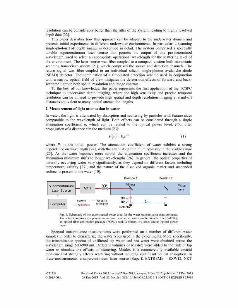
Fig. 1. Schematic of the experimental setup used for the water transmittance measurements. The setup comprises a supercontinuum laser source, an acousto-optic tunable filter (AOTF), an optical fiber collimation package (FCP), a tank, a mirror, two irises and an optical power meter.

Spectral transmittance measurements were performed on a number of different water samples in order to characterize the water types used in the experiments. More specifically, the transmittance spectra of unfiltered tap water and sea water were obtained across the wavelength range 500-900 nm. Different volumes of Maalox were added to the tank of tap water to simulate the effects of scattering. Maalox is a commercially available antacid medicine that strongly affects scattering without inducing significant optical absorption. In these measurements, a supercontinuum laser source (SuperK EXTREME – EXW12, NKT


Photonics, Denmark) was used in conjunction with an acousto-optic tunable filter (AOTF) in order to select a single wavelength. At each wavelength the laser source had a spectral Full Width at Half Maximum (FWHM) of approximately 5 nm in the range 500-900 nm for each individual transmittance measurement. As shown schematically in Fig. 1, the collimated laser beam (approximately 4 mm in diameter) was directed into a 110 liter capacity tank (1750 mm long, 250 mm high, 250 mm wide). A mirror was placed in the tank of water at an angle of 45° to the beam and directed the beam out through the side wall of the tank. Optical powers were recorded with a silicon detector (Newport Power Meter 1830C and 818-UV detector head). First of all, the optical power readings were taken at the Position 1, as shown in Fig. 1. For each optical power measurement, two separated irises were aligned in front of the detector. This configuration allows the laser beam to efficiently pass, but blocks most of the forward-scattered light that could cause an over-estimation of the power of the transmitted light. The optical power was then measured with the mirror in Position 2 and the transmittance over exactly 1 meter of propagation within the transmission medium was calculated from the ratio of these two power values. The medium’s attenuation coefficient for that wavelength was then calculated using Eq. (1). By repeating these optical power measurements at a series of different discrete wavelengths, we ascertained the transmittance and attenuation length spectra.

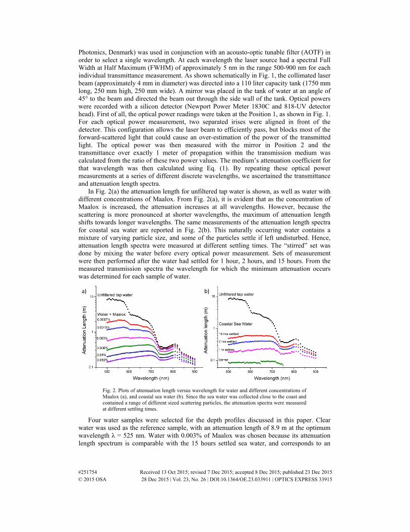
In Fig. 2(a) the attenuation length for unfiltered tap water is shown, as well as water with different concentrations of Maalox. From Fig. 2(a), it is evident that as the concentration of Maalox is increased, the attenuation increases at all wavelengths. However, because the scattering is more pronounced at shorter wavelengths, the maximum of attenuation length shifts towards longer wavelengths. The same measurements of the attenuation length spectra for coastal sea water are reported in Fig. 2(b). This naturally occurring water contains a mixture of varying particle size, and some of the particles settle if left undisturbed. Hence, attenuation length spectra were measured at different settling times. The “stirred” set was done by mixing the water before every optical power measurement. Sets of measurement were then performed after the water had settled for 1 hour, 2 hours, and 15 hours. From the measured transmission spectra the wavelength for which the minimum attenuation occurs was determined for each sample of water.

Fig. 2. Plots of attenuation length versus wavelength for water and different concentrations of Maalox (a), and coastal sea water (b). Since the sea water was collected close to the coast and contained a range of different sized scattering particles, the attenuation spectra were measured at different settling times.

Four water samples were selected for the depth profiles discussed in this paper. Clear water was used as the reference sample, with an attenuation length of 8.9 m at the optimum wavelength λ = 525 nm. Water with 0.003% of Maalox was chosen because its attenuation length spectrum is comparable with the 15 hours settled sea water, and corresponds to an


attenuation length of 0.7 m at the optimum wavelength λ = 585 nm. To simulate a highly attenuating environment, water with 0.01%, and 0.012%, of Maalox were used to characterize the system. For both concentrations the transmission peak is at λ = 690 nm, corresponding to attenuation lengths of 0.3 m and 0.21 m respectively.

3. Underwater depth imaging system and results

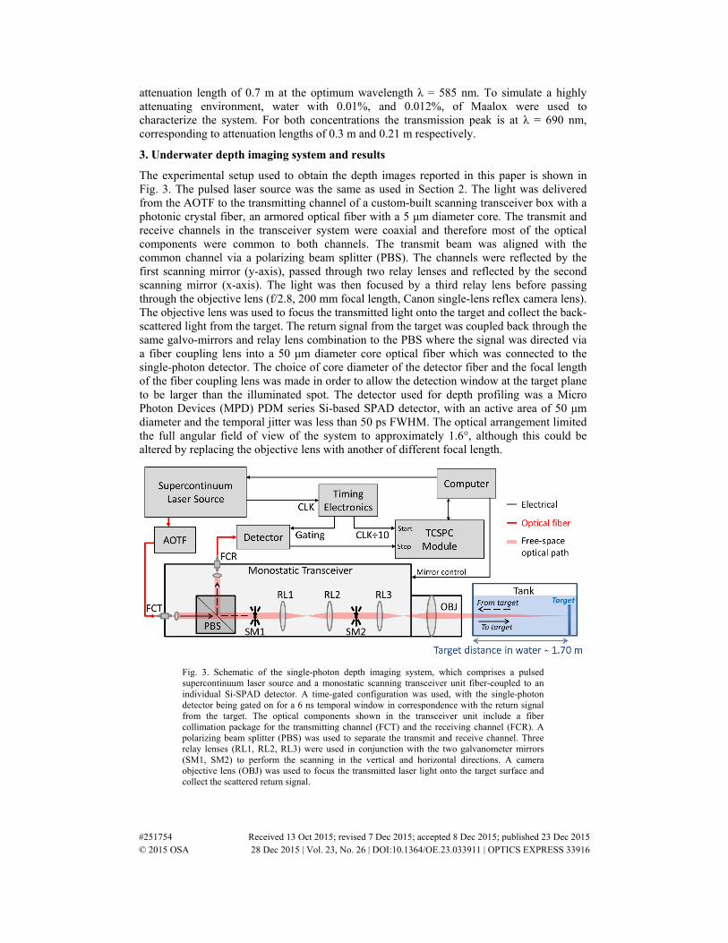
The experimental setup used to obtain the depth images reported in this paper is shown in Fig. 3. The pulsed laser source was the same as used in Section 2. The light was delivered from the AOTF to the transmitting channel of a custom-built scanning transceiver box with a photonic crystal fiber, an armored optical fiber with a 5 μm diameter core. The transmit and receive channels in the transceiver system were coaxial and therefore most of the optical components were common to both channels. The transmit beam was aligned with the common channel via a polarizing beam splitter (PBS). The channels were reflected by the first scanning mirror (y-axis), passed through two relay lenses and reflected by the second scanning mirror (x-axis). The light was then focused by a third relay lens before passing through the objective lens (f/2.8, 200 mm focal length, Canon single-lens reflex camera lens). The objective lens was used to focus the transmitted light onto the target and collect the back-scattered light from the target. The return signal from the target was coupled back through the same galvo-mirrors and relay lens combination to the PBS where the signal was directed via a fiber coupling lens into a 50 μm diameter core optical fiber which was connected to the single-photon detector. The choice of core diameter of the detector fiber and the focal length of the fiber coupling lens was made in order to allow the detection window at the target plane to be larger than the illuminated spot. The detector used for depth profiling was a Micro Photon Devices (MPD) PDM series Si-based SPAD detector, with an active area of 50 μm diameter and the temporal jitter was less than 50 ps FWHM. The optical arrangement limited the full angular field of view of the system to approximately 1.6°, although this could be altered by replacing the objective lens with another of different focal length.

Fig. 3. Schematic of the single-photon depth imaging system, which comprises a pulsed supercontinuum laser source and a monostatic scanning transceiver unit fiber-coupled to an individual Si-SPAD detector. A time-gated configuration was used, with the single-photon detector being gated on for a 6 ns temporal window in correspondence with the return signal from the target. The optical components shown in the transceiver unit include a fiber collimation package for the transmitting channel (FCT) and the receiving channel (FCR). A polarizing beam splitter (PBS) was used to separate the transmit and receive channel. Three relay lenses (RL1, RL2, RL3) were used in conjunction with the two galvanometer mirrors (SM1, SM2) to perform the scanning in the vertical and horizontal directions. A camera objective lens (OBJ) was used to focus the transmitted laser light onto the target surface and collect the scattered return signal.


Due to the monostatic optical configuration used in the transceiver and the high sensitivity of the single-photon detector, the optical back-reflections in the system can be significant, contributing to the overall dead-time of the detection system and reducing the transceiver effectiveness. To avoid detection of these internal back-reflections, a time-gated detection scheme was used. The detector was activated for a temporal window of 6 ns in correspondence with the approximate expected return time from the target, in order to temporally gate out these unwanted back-reflections. In these experiments, a 19.5 MHz laser repetition rate was used, and an average optical power (measured just before the objective lens) was chosen in the range 0.8 nW to 950 μW. The laser source provided an electrical synchronization signal to trigger both the TCSPC module (PicoHarp 300, PicoQuant GmbH, Germany) and the detector gating. A limitation of the TCSPC hardware module meant that the frequency of its clock input could not exceed 10 MHz and as a result the synchronization signal was divided by a factor of 10. Consequently, this modified the number of optical pulses per start signal to 10, and hence every histogram has 10 return peaks from the target.

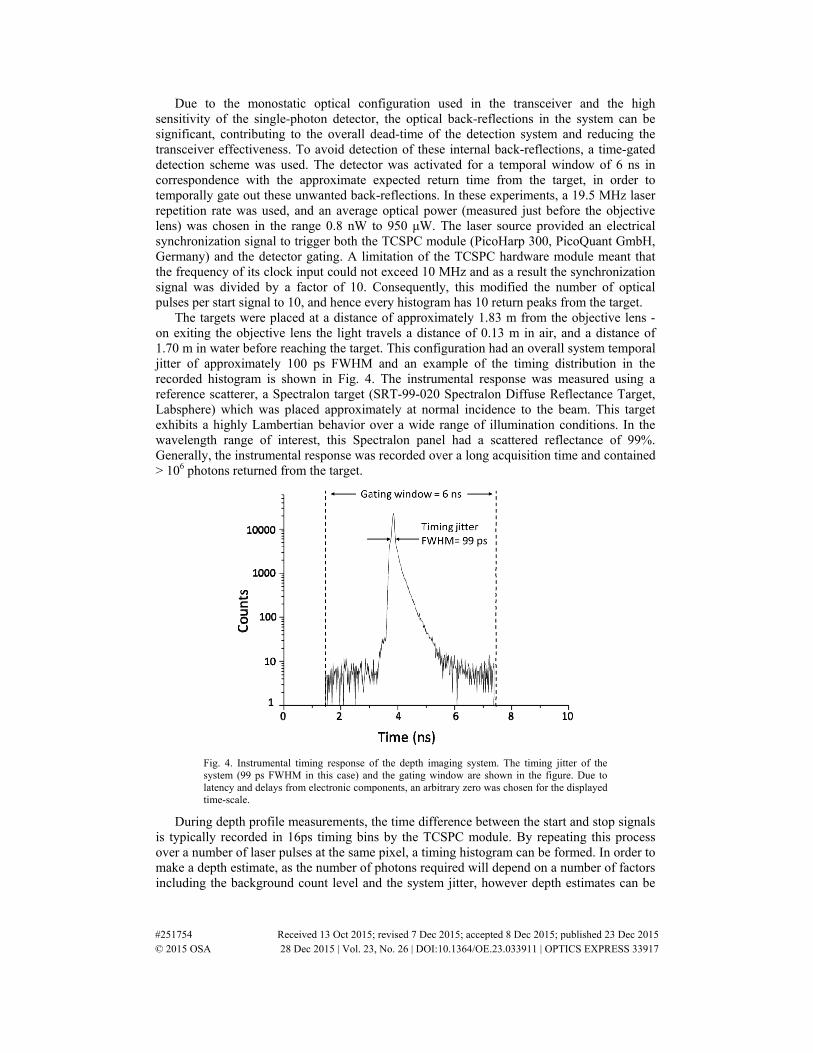
The targets were placed at a distance of approximately 1.83 m from the objective lens - on exiting the objective lens the light travels a distance of 0.13 m in air, and a distance of 1.70 m in water before reaching the target. This configuration had an overall system temporal jitter of approximately 100 ps FWHM and an example of the timing distribution in the recorded histogram is shown in Fig. 4. The instrumental response was measured using a reference scatterer, a Spectralon target (SRT-99-020 Spectralon Diffuse Reflectance Target, Labsphere) which was placed approximately at normal incidence to the beam. This target exhibits a highly Lambertian behavior over a wide range of illumination conditions. In the wavelength range of interest, this Spectralon panel had a scattered reflectance of 99%. Generally, the instrumental response was recorded over a long acquisition time and contained > 106 photons returned from the target.

Fig. 4. Instrumental timing response of the depth imaging system. The timing jitter of the system (99 ps FWHM in this case) and the gating window are shown in the figure. Due to latency and delays from electronic components, an arbitrary zero was chosen for the displayed time-scale.

During depth profile measurements, the time difference between the start and stop signals is typically recorded in 16ps timing bins by the TCSPC module. By repeating this process over a number of laser pulses at the same pixel, a timing histogram can be formed. In order to make a depth estimate, as the number of photons required will depend on a number of factors including the background count level and the system jitter, however depth estimates can be


made with fewer than 10 photons returned from the target using the cross-correlation approach [20]. At each individual pixel, the histogram was folded into a single peak and a cross-correlation C was performed between a normalized instrumental response R with r timing bins and the acquired timing histogram of the returned photon counts H with h timing bins, as

1

r

i i j jj

C H R+=

= × (2)

with i varying in [ ],r h− . The highest cross-correlation for each pixel reveals the time-of-

flight to the target with respect to the reference for that individual pixel. It is worth noting that this cross-correlation approach is not ideal for multiple returns or returns from an angled target, where time-of-flight differences can alter the temporal profile of the signal return and introduce additional error into the depth measurement. By collecting this time-of-flight information for all of the pixels, a depth image for the scanned field of view was then estimated. In all the measurements presented in this paper, the depth profiles were formed using this pixel-wise data processing approach and no attempt at using spatial correlations to process the depth image was made. Such image processing approaches will be the subject of future work, but preliminary results indicate that appropriate image processing algorithms can significantly reduce the acquisition times required for image reconstruction [28, 29], thus making a clear contribution to the future practicality of this depth image approach.

One potential disadvantage of using periodic optical pulses is range ambiguity which occurs when the round-trip time is greater than the period between optical pulses, leading to uncertainty in the specific pulse which originated the time-of-flight event. In the measurements presented in this paper, the short target distance meant that range ambiguity was not an issue. However as the target distance increases beyond 5-10 meters, there is the potential of range ambiguity at the laser repetition frequencies used in these experiments. One solution is to pulse the laser at a lower repetition frequency when illuminating at least some of the pixels. This will enable the absolute range to be determined for those pixels, and this can then be used to remove any range ambiguity for the rest of the depth profile. In addition, previous research has demonstrated how such ambiguity can also be fully eliminated by use of a pseudo-random pattern-matching technique [30, 31].

A number of depth profile measurements were taken of different target objects at an overall stand-off distance of approximately 1.83 m. During the course of the measurements the laboratory was kept in dark conditions, to avoid ambient light contributing to the background level of the detector. Under these conditions, the detector background level was approximately 10 counts per second. The level of surface detail recovered from the depth profile depends on a number of factors, including the spacing of the illuminated pixels at the target and the number of photon events recorded at each pixel, which is dependent on the acquisition time. Hence, for the measurements discussed in this paper, different pixel formats and acquisition times per pixel will be investigated. In each case, the cross-correlation approach was performed using an instrumental response recorded from the Spectralon panel placed at the same standoff distance as the target, and using the same 6 ns detection gate width used for the target measurements. The cross-correlation was performed on data in the 6 ns gate format and no additional post-processing of the data (e.g. additional removal of unused parts of the detection window) was performed prior to the cross-correlation stage.

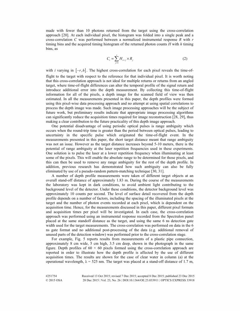
For example, Fig. 5 reports results from measurements of a plastic pipe connection, approximately 8 cm wide, 5 cm high, 3.5 cm deep, shown in the photograph in the same figure. Depth profiles of 60 × 60 pixels formed using the cross-correlation approach are reported in order to illustrate how the depth profile is affected by the use of different acquisition times. The results are shown for the case of clear water in column (a) at the operational wavelength, λ = 525 nm. The target was placed at a stand-off distance of 1.7 m,


equivalent to 0.2 attenuation lengths in clear water. Four different per-pixel acquisition times were used, 0.5, 1, 10, 100 ms, with a very low average power, 8 nW. The same target was measured in water with 0.003% of Maalox (λ = 585 nm), at a stand-off distance of 1.2 attenuation lengths, using the same average power and acquisition times, and the depth profiles for this case are shown in column (b). From these results it is evident that even at the shortest acquisition times of 0.5 ms per pixel it is possible to resolve the shape of the target in clear water, although some pixels have insufficient returns for a distinct time-of-flight measurement to be determined from the pixel-wise cross-correlation procedure. When the scattering level is increased, the depth profile degrades significantly as the per-pixel acquisition time is reduced, and at 0.5 ms acquisition time the shape of the pipe cannot be discerned from the depth image when using this pixel-wise data analysis approach.

Fig. 5. The photograph shows the target used for the depth profile measurements, a plastic pipe (approximately 8 cm wide, 5 cm high, and 3.5 cm deep) placed on a red Lego block in the water tank. Depth profile images from measurements performed in clear water at λ = 525 nm (column (a)) and water with 0.003% of Maalox at λ = 585 nm (column (b)) using 60 × 60 pixels in all cases. Clear water (column (a)) corresponded to 0.2 attenuation lengths from transceiver to target, whilst column (b) corresponded to 1.2 attenuation lengths. An average power of just 8 nW was used in all measurements, and different per-pixel acquisition times are shown (of 0.5 ms, 1 ms, 10 ms and 100 ms) in order to investigate how the depth profile changes using different acquisition times.

Figure 6 illustrates 256 × 256 pixel depth scans of the plastic pipe. The depth profile and a plot of the number of photons per pixel (intensity map) taken in clear water are shown in Figs. 6(a) and 6(b) respectively. A wavelength of 525 nm was used in this scan, with an acquisition time of 30 ms per pixel and only 8.7 nW of average optical power. It is evident


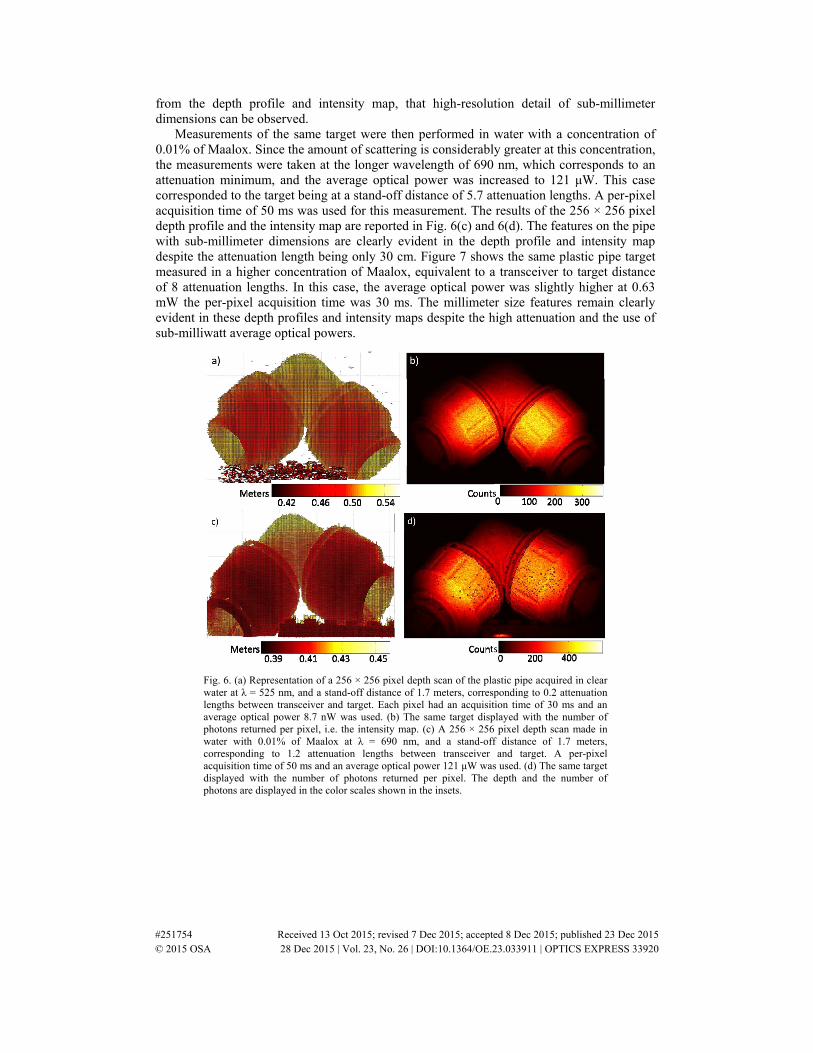
from the depth profile and intensity map, that high-resolution detail of sub-millimeter dimensions can be observed.

Measurements of the same target were then performed in water with a concentration of 0.01% of Maalox. Since the amount of scattering is considerably greater at this concentration, the measurements were taken at the longer wavelength of 690 nm, which corresponds to an attenuation minimum, and the average optical power was increased to 121 μW. This case corresponded to the target being at a stand-off distance of 5.7 attenuation lengths. A per-pixel acquisition time of 50 ms was used for this measurement. The results of the 256 × 256 pixel depth profile and the intensity map are reported in Fig. 6(c) and 6(d). The features on the pipe with sub-millimeter dimensions are clearly evident in the depth profile and intensity map despite the attenuation length being only 30 cm. Figure 7 shows the same plastic pipe target measured in a higher concentration of Maalox, equivalent to a transceiver to target distance of 8 attenuation lengths. In this case, the average optical power was slightly higher at 0.63 mW the per-pixel acquisition time was 30 ms. The millimeter size features remain clearly evident in these depth profiles and intensity maps despite the high attenuation and the use of sub-milliwatt average optical powers.

Fig. 6. (a) Representation of a 256 × 256 pixel depth scan of the plastic pipe acquired in clear water at λ = 525 nm, and a stand-off distance of 1.7 meters, corresponding to 0.2 attenuation lengths between transceiver and target. Each pixel had an acquisition time of 30 ms and an average optical power 8.7 nW was used. (b) The same target displayed with the number of photons returned per pixel, i.e. the intensity map. (c) A 256 × 256 pixel depth scan made in water with 0.01% of Maalox at λ = 690 nm, and a stand-off distance of 1.7 meters, corresponding to 1.2 attenuation lengths between transceiver and target. A per-pixel acquisition time of 50 ms and an average optical power 121 μW was used. (d) The same target displayed with the number of photons returned per pixel. The depth and the number of photons are displayed in the color scales shown in the insets.


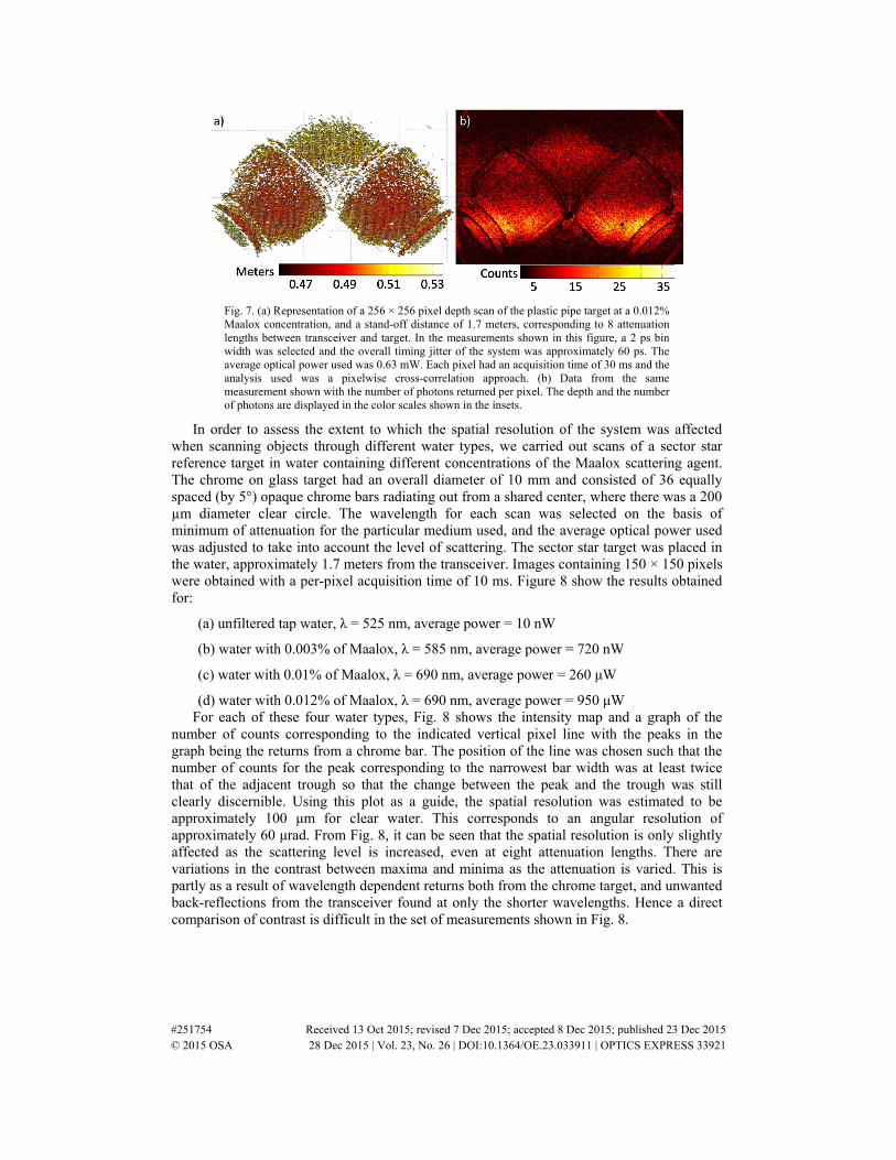
Fig. 7. (a) Representation of a 256 × 256 pixel depth scan of the plastic pipe target at a 0.012% Maalox concentration, and a stand-off distance of 1.7 meters, corresponding to 8 attenuation lengths between transceiver and target. In the measurements shown in this figure, a 2 ps bin width was selected and the overall timing jitter of the system was approximately 60 ps. The average optical power used was 0.63 mW. Each pixel had an acquisition time of 30 ms and the analysis used was a pixelwise cross-correlation approach. (b) Data from the same measurement shown with the number of photons returned per pixel. The depth and the number of photons are displayed in the color scales shown in the insets.

In order to assess the extent to which the spatial resolution of the system was affected when scanning objects through different water types, we carried out scans of a sector star reference target in water containing different concentrations of the Maalox scattering agent. The chrome on glass target had an overall diameter of 10 mm and consisted of 36 equally spaced (by 5°) opaque chrome bars radiating out from a shared center, where there was a 200 µm diameter clear circle. The wavelength for each scan was selected on the basis of minimum of attenuation for the particular medium used, and the average optical power used was adjusted to take into account the level of scattering. The sector star target was placed in the water, approximately 1.7 meters from the transceiver. Images containing 150 × 150 pixels were obtained with a per-pixel acquisition time of 10 ms. Figure 8 show the results obtained for:

(a) unfiltered tap water, λ = 525 nm, average power = 10 nW

(b) water with 0.003% of Maalox, λ = 585 nm, average power = 720 nW

(c) water with 0.01% of Maalox, λ = 690 nm, average power = 260 μW

(d) water with 0.012% of Maalox, λ = 690 nm, average power = 950 μW For each of these four water types, Fig. 8 shows the intensity map and a graph of the

number of counts corresponding to the indicated vertical pixel line with the peaks in the graph being the returns from a chrome bar. The position of the line was chosen such that the number of counts for the peak corresponding to the narrowest bar width was at least twice that of the adjacent trough so that the change between the peak and the trough was still clearly discernible. Using this plot as a guide, the spatial resolution was estimated to be approximately 100 μm for clear water. This corresponds to an angular resolution of approximately 60 μrad. From Fig. 8, it can be seen that the spatial resolution is only slightly affected as the scattering level is increased, even at eight attenuation lengths. There are variations in the contrast between maxima and minima as the attenuation is varied. This is partly as a result of wavelength dependent returns both from the chrome target, and unwanted back-reflections from the transceiver found at only the shorter wavelengths. Hence a direct comparison of contrast is difficult in the set of measurements shown in Fig. 8.


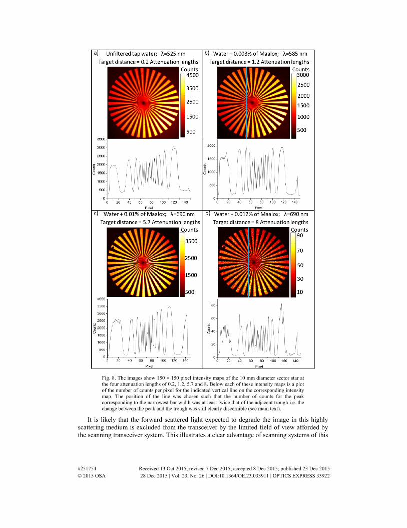
Fig. 8. The images show 150 × 150 pixel intensity maps of the 10 mm diameter sector star at the four attenuation lengths of 0.2, 1.2, 5.7 and 8. Below each of these intensity maps is a plot of the number of counts per pixel for the indicated vertical line on the corresponding intensity map. The position of the line was chosen such that the number of counts for the peak corresponding to the narrowest bar width was at least twice that of the adjacent trough i.e. the change between the peak and the trough was still clearly discernible (see main text).

It is likely that the forward scattered light expected to degrade the image in this highly scattering medium is excluded from the transceiver by the limited field of view afforded by the scanning transceiver system. This illustrates a clear advantage of scanning systems of this


type which inherently spatially filter out the forward-scattered return signal, predominantly allowing light not scattered by the transmission medium into the detection system.

4. LiDAR equation model

A model based on the photon-counting version of the LiDAR range equation [6] was developed to evaluate the system’s time-of-flight ranging performance in water. Several intrinsic and extrinsic parameters that contribute to the number of counts in the peak were included. Intrinsic parameters consider the attenuation of each optical element, detector response, and operational parameters. Extrinsic parameters take in account the environmental attenuation estimated from the transmittance spectra measured in Section 2. The model gives the number of photons in the highest histogram bin in the return peak based on the equation

222

rOut Lensp Dwell Int Det

P An t e C C

hc Rαλ ρ η

π−= (3)

where Outr P hcγ λ= is the average photon emission rate (h is the Planck’s constant and c is

the speed of light), proportional to the average output power of the laser POut and the wavelength of light used in the measurement, λ. The dwell time tDwell is the duration of the acquisition time at each pixel. The system collects just a fraction of the light which is assumed to be scattered isotropically by the target, so geometric considerations must be included in the equation. An objective lens of area ALens collects the fraction

24

C Lens

S

I A

I Rπ= (4)

of the intensity IS scattered in the solid angle 4π by a target at a stand-off distance R [32]. It is assumed that the spatial resolution remains similar as the attenuation length increases, and that the laser illumination spot is fully encompassed by the detection window of the transceiver system.

The model is calibrated on experimental measurements of returns from the Spectralon target. The target reflectance (ρ) is the percentage of light that is scattered on reflection by the target., The Spectralon panel has a scattered reflectance of 99%, with negligible transmittance. Hence only the back-scattered radiation representing half of the overall solid angle possible has to be considered. In the experimental setup used, the light travels a short distance d in air, from the objective lens to the window of the tank. Then it travels a distance r in water, from the entrance window of the tank to the target. Because of the change in the refractive index of the two different media, the distance to consider in the geometric factor is R = d + nr, where n is the refractive index of water. Then the geometric factor included in the equation is

( )2

2C Lens

S

I A

I d nrπ=

+ (5)

The exponential term in Eq. (3) considers the attenuation of light in the water, as discussed before in section 2. The internal system attenuation coefficient CInt represents losses due to the individual optical elements, coupling losses and possible misalignment of the system. The two coefficients CDet and η describe the detector characteristics. In particular, the temporal detector response coefficient CDet is the ratio between the number of counts in the highest bin in peak and the total number of photons in the peak. It is empirically determined and depends on the detector properties and the bin width used. The coefficient η is the detector’s single-photon detection efficiency [33]. For each configuration, the background noise level was measured. Several histograms with different integration times


were recorded with the detector in free running mode in the absence of laser radiation to accurately determine the average background counts per bin nb [30]:

Reb Dwell p Binn t Bf t= (6)

where B is the total number of background counts in the histogram, fRep the laser repetition rate, tBin the histogram bin size. The number of photons in the highest bin in peak np and the average number of background counts per bin were used to estimate the signal-to-noise ratio (SNR) as [34]:

p

p b

nSNR

n n=

+ (7)

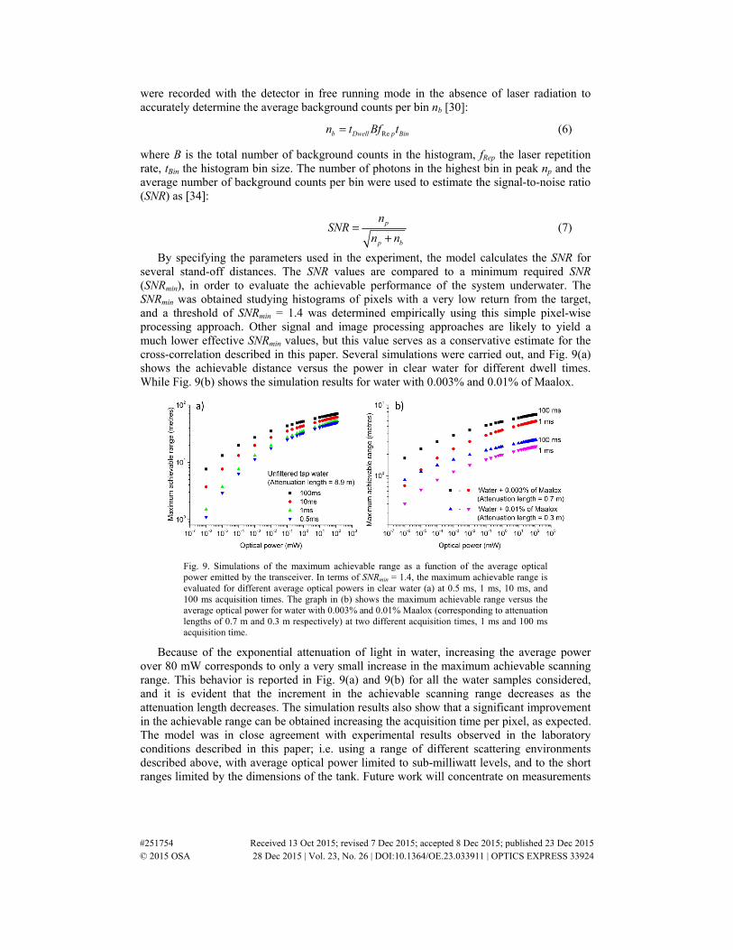
By specifying the parameters used in the experiment, the model calculates the SNR for several stand-off distances. The SNR values are compared to a minimum required SNR (SNRmin), in order to evaluate the achievable performance of the system underwater. The SNRmin was obtained studying histograms of pixels with a very low return from the target, and a threshold of SNRmin = 1.4 was determined empirically using this simple pixel-wise processing approach. Other signal and image processing approaches are likely to yield a much lower effective SNRmin values, but this value serves as a conservative estimate for the cross-correlation described in this paper. Several simulations were carried out, and Fig. 9(a) shows the achievable distance versus the power in clear water for different dwell times. While Fig. 9(b) shows the simulation results for water with 0.003% and 0.01% of Maalox.

Fig. 9. Simulations of the maximum achievable range as a function of the average optical power emitted by the transceiver. In terms of SNRmin = 1.4, the maximum achievable range is evaluated for different average optical powers in clear water (a) at 0.5 ms, 1 ms, 10 ms, and 100 ms acquisition times. The graph in (b) shows the maximum achievable range versus the average optical power for water with 0.003% and 0.01% Maalox (corresponding to attenuation lengths of 0.7 m and 0.3 m respectively) at two different acquisition times, 1 ms and 100 ms acquisition time.

Because of the exponential attenuation of light in water, increasing the average power over 80 mW corresponds to only a very small increase in the maximum achievable scanning range. This behavior is reported in Fig. 9(a) and 9(b) for all the water samples considered, and it is evident that the increment in the achievable scanning range decreases as the attenuation length decreases. The simulation results also show that a significant improvement in the achievable range can be obtained increasing the acquisition time per pixel, as expected. The model was in close agreement with experimental results observed in the laboratory conditions described in this paper; i.e. using a range of different scattering environments described above, with average optical power limited to sub-milliwatt levels, and to the short ranges limited by the dimensions of the tank. Future work will concentrate on measurements


performed with a submerged transceiver unit to verify the model predictions at higher optical power levels and significantly longer distances.

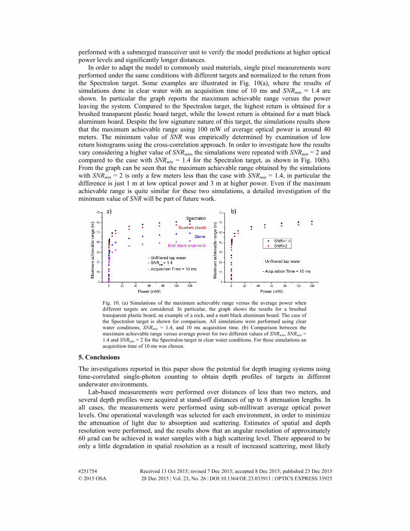
In order to adapt the model to commonly used materials, single pixel measurements were performed under the same conditions with different targets and normalized to the return from the Spectralon target. Some examples are illustrated in Fig. 10(a), where the results of simulations done in clear water with an acquisition time of 10 ms and SNRmin = 1.4 are shown. In particular the graph reports the maximum achievable range versus the power leaving the system. Compared to the Spectralon target, the highest return is obtained for a brushed transparent plastic board target, while the lowest return is obtained for a matt black aluminum board. Despite the low signature nature of this target, the simulations results show that the maximum achievable range using 100 mW of average optical power is around 40 meters. The minimum value of SNR was empirically determined by examination of low return histograms using the cross-correlation approach. In order to investigate how the results vary considering a higher value of SNRmin, the simulations were repeated with SNRmin = 2 and compared to the case with SNRmin = 1.4 for the Spectralon target, as shown in Fig. 10(b). From the graph can be seen that the maximum achievable range obtained by the simulations with SNRmin = 2 is only a few meters less than the case with SNRmin = 1.4, in particular the difference is just 1 m at low optical power and 3 m at higher power. Even if the maximum achievable range is quite similar for these two simulations, a detailed investigation of the minimum value of SNR will be part of future work.

Fig. 10. (a) Simulations of the maximum achievable range versus the average power when different targets are considered. In particular, the graph shows the results for a brushed transparent plastic board, an example of a rock, and a matt black aluminum board. The case of the Spectralon target is shown for comparison. All simulations were performed using clear water conditions, SNRmin = 1.4, and 10 ms acquisition time. (b) Comparison between the maximum achievable range versus average power for two different values of SNRmin, SNRmin = 1.4 and SNRmin = 2 for the Spectralon target in clear water conditions. For these simulations an acquisition time of 10 ms was chosen.

5. Conclusions

The investigations reported in this paper show the potential for depth imaging systems using time-correlated single-photon counting to obtain depth profiles of targets in different underwater environments.

Lab-based measurements were performed over distances of less than two meters, and several depth profiles were acquired at stand-off distances of up to 8 attenuation lengths. In all cases, the measurements were performed using sub-milliwatt average optical power levels. One operational wavelength was selected for each environment, in order to minimize the attenuation of light due to absorption and scattering. Estimates of spatial and depth resolution were performed, and the results show that an angular resolution of approximately 60 µrad can be achieved in water samples with a high scattering level. There appeared to be only a little degradation in spatial resolution as a result of increased scattering, most likely


due to the limited field of view afforded by the scanning system. High resolution scans show that sub-millimeter depth resolution is attained despite the high level of scattering in the medium. Further work will be necessary to investigate the relationship between scattering level and spatial resolution in this type of scanning transceiver, especially at longer ranges. The limited field of view has proved advantageous in this implementation of underwater single-photon depth imaging, and such an advantage will not be straightforward to achieve in a single-photon detector array implementation [35]. In a detector array, the forward and backscattered radiation is likely to degrade contrast and spatial resolution, although this could be mitigated to some extent by using structured illumination of the target surface.

The extension of this imaging approach to long ranges will mean some adaptations to the detector gating approach, in order not to miss targets in the temporal windows outside the detector gate. The simplest approach is to gate the detector off only during the initial pass through the system to avoid the transceiver back-reflections. Another approach is to move the detector gate with respect to the laser start signal across the full return temporal range. In the event of a signal return being detected, the detector gate would be fixed in the vicinity of the return signal to allow the depth imaging measurement to be performed. Other hybrid detection approaches could be used, such as combining a sonar measurement for an initial depth estimate, followed by full single-photon depth imaging using the detector gated near the initial depth estimate.

A model based on the LiDAR equation was developed and calibrated using the laboratory results for this depth imaging system. The model evaluates the system’s time-of-flight ranging performance in water under a variety of scatter conditions. The simulations carried out show how the maximum achievable scanning range depends on several factors, including average optical power, acquisition time and minimum SNR value. It seems that, if the average optical power is in the 10’s mW it should be possible to perform high-speed depth images at distances of 30-60 meters in clear water, even with relatively low signature targets. In addition, the simulations results suggest that the time-of-flight system described, when used in conjunction with the appropriate laser source, is capable of depth profiling a target at a stand-off distance equivalent of up to ten attenuation lengths, under a limited set of conditions.

Further studies over long distances will be performed using submerged transceivers, in conjunction with more advanced signal and image processing approaches, in order to optimize the maximum achievable scanning range of the system. Work on image processing using spatial correlation approaches are likely to yield significant reductions in the acquisition times required to reconstruct depth images from sparse photon data.

Acknowledgments

The authors acknowledge the support of the DSTL National PhD Scheme and the UK Engineering and Physical Sciences Research Council (EPSRC) Platform Grant no. No. EP/K015338/1, in addition to projects EP/M01326X/1, EP/M006514/1 and EP/N003446/1.


underwater depth imaging using time- correlated single ... · underwater depth imaging using...

Documents