1

Understanding the Dynamic Mho Distance Characteristic

Donald D. Fentie, Schweitzer Engineering Laboratories, Inc. 2350 NE Hopkins Court, Pullman, WA 99163 USA, +1.509.332.1890

Abstract—In order to retain dependability and security in cases of close-in faults when the loop voltage is zero, mho distance elements use cross-phase and/or memory polarization. Polarization techniques in distance elements cause the mho distance characteristic to dynamically expand and then contract as the polarization memory decays during a fault. The dynamic behavior of this mho element continues to be a confusing topic to many engineers. Many papers and text books written on the subject are mired in long derivations and produce equations that can seem abstract.

This paper bridges the theory with familiar phasor diagrams and visual aids to promote an intuitive understanding of the dynamic mho expansion during balanced and unbalanced faults in the forward and reverse direction. We examine the dynamic mho expansion for common fault types, load flow conditions, and under typical relay test scenarios. We emphasize visualizing the expansion for positive-sequence memory polarization while demonstrating its practical benefits in terms of security, directionality, and increased resistive coverage.

I. INTRODUCTION Mho distance elements continue to be popular for

transmission protection worldwide. In the past, as relay technology improved from coils and discs to microprocessors, improvements were made to algorithms, polarization, and response times. The fundamental principles of mho distance elements still apply, and there is continued interest in understanding this seemingly simple protective element.

This paper discusses the mho element and dynamic expansion characteristics for positive-sequence polarization during testing, load flow, and fault conditions. It also discusses element security during single-pole open and series-capacitor applications. This paper departs from many other papers that present mathematical equations governing mho expansion by instead emphasizing visualization to promote a more intuitive understanding [1] [7] [9] [10].

II. BACKGROUND A self-polarized mho element for the system shown in

Fig. 1(a) is represented as a circle on the impedance plane in Fig. 1(b). The diameter of this circle extends from the origin of the plane to the relay reach setting Zr on the bolted fault locus. The relay calculates the impedance Z by using the measured voltage and current phasors at each processing interval. The mho element restrains until Z plots inside the circle.

ZS1 mZL1 (1 – m)ZL1 ZR1

RF

ES ER

Relay

(a)

3

2

1

1 2–1

X

R

Z

Zr

Operating Restrainingm ∙ Zr

–2

(b)

Fig. 1 Line fault at 50 percent of reach (m = 0.5 p.u.): (a) System one-line diagram, (b) Mho characteristic.

If we assume no arc impedance, the calculated impedance for a fault at the relay is zero. If the measured impedance is plotted for a three-phase fault at each point along the transmission line, it will produce a bolted fault locus with the same angle as the transmission-line impedance. At a certain distance from the relay, Z equals the mho reach Zr. All points on the bolted fault locus between the relay reach point and the origin are enclosed within the area of operation.

A. The Self-Polarized Mho Circle Microprocessor relays require an efficient method for

determining if a measured impedance is inside the mho operating characteristic. One technique is to examine known phase angle relationships, as shown in Fig. 2. Note that the measured impedance Z in this example does not lie on the bolted fault locus because of arc resistance.

2

3

2

1

1 2–1

X

R

Z

dZZr

δ < 90°

–2

(a)

3

2

1

1 2–1

X

R

Z

dZZr

δ = 90°

–2

(b)

3

2

1

1 2–1

X

R

Z

dZ

Zr

δ > 90°

–2

(c)

Fig. 2 Impedance vectors for faults (a) Inside zone, (b) At reach point, (c) Outside zone.

Vector dZ defines the impedance between the fault and the relay reach point as shown in (1). = −rdZ Z Z (1)

When the measured impedance is inside the mho circle, the angle δ, defined as θdZ − θZ, is between −90 and +90 degrees. The diameter of the circle is defined by Vector Zr, which splits the mho into a left and right side. When the impedance lies directly on the edge of the left half or right half of the mho, δ equals −90 and +90 degrees, respectively, as shown in Fig. 3.

All other angle differences signify that the impedance is outside the mho circle. These three conditions are shown in (2), (3), and (4).

Operate (inside mho):

90 arg 90 − ° < < ° dZZ

(2)

Restrain (outside mho):

90 arg 90 ° < < − ° dZZ

(3)

Indeterminate (on the mho circle):

arg 90 = ± ° dZZ

(4)

3

2

1

1 2–1

X

R

Z1

dZ1

Zr

δ1

dZ3

Z3

Z2

δ3

δ2 dZ2

–2

Fig. 3 Right-angle property of a circle.

The impedance from the relay to the reach point determines the diameter of the mho circle. Vectors dZ and Z will always be at right angles to each other when the impedance point lies on the mho circle. The angle comparison is typically shown in terms of measured voltage by multiplying the numerator and denominator in (4) by the faulted loop current I, as shown in (5).

arg arg arg− ⋅ − = =

r rZ Z I Z VdZZ Z V

(5)

Although (5) is mathematically correct, it is not a computationally efficient representation. We can simplify the equation by using comparators, as discussed in the next subsection.

B. Comparators A phase comparator determines if the angle difference

between two phasors is within a specified range [1]. In addition to (5), the angle difference between dZ and Z can be represented as shown in (6).

( )*arg ∠ ⋅ ∠ = −dZ Z dZ ZdZ Zθ θ θ θ (6)

A measured impedance is inside the mho circle when the result of (6) is between −90 and +90 degrees. The cosine function with no phase shift is positive between −90 and +90 degrees, and thus it makes an excellent comparator for determining whether the impedance is within the mho element. If the cosine of the angle difference between dZ and Z is positive, the impedance is inside the mho element.

3

We can use Euler’s formula to rewrite the expression inside the brackets of (6), separating it into real and imaginary components, as shown in (7).

( ) ( )( )* cos sin⋅ = ⋅ ⋅ − + ⋅ −dZ Z dZ ZdZ Z dZ Z jθ θ θ θ (7)

Taking the real part of (7) yields the cosine comparator (8), the result of which is positive if the impedance plots inside the mho circle.

( )*Re cos 0 ⋅ = ⋅ ⋅ − > dZ ZdZ Z dZ Z θ θ (8)

Substituting (1) into (8) gives (9):

( ) *Re 0 − ⋅ > rZ Z Z (9)

Equation (9) is often expressed in terms of voltage, as shown in (10), by multiplying each term by current, where V is the measured voltage at the relay and I is the fault loop current, as described in Section III, Subsection A [1].

( ) *Re 0 ⋅ − ⋅ > rZ I V V (10)

The mho element in Fig. 4 is represented in terms of voltage on the complex plane.

30

20

10

10 20–10

I ∙ X

I ∙ R

V

dV

I ∙ Zr

δ

–20

40

50

30

Fig. 4 Mho element in terms of voltage.

We can improve (9) so that it projects or maps Z to the bolted fault locus as a scalar quantity that we can then compare directly with a scalar reach point on a number line [1]. By setting (9) equal to zero, as shown in (11), we define a circle that passes through the origin and Z. The diameter of the circle lies along the line angle.

( ) *Re 0 − ⋅ = rZ Z Z (11)

We can solve (11) for the magnitude of Zr to find the mapped impedance, as shown in (12), (13), and (14).

( ) *Re 0 ∠ − ⋅ = rr ZZ Z Zθ (12)

* *Re Re 0 ∠ ⋅ − ⋅ = rr ZZ Z Z Zθ (13)

*

*

Re

Re 1

⋅ = ∠ ⋅ r

rZ

Z ZZ

Zθ (14)

Zr can also be mapped as a negative number in (14) by removing the absolute value sign, as shown in (15).

*

*

Re

Re 1

⋅ = ∠ ⋅ r

rZ

Z ZZ

Zθ (15)

Equations (16) and (17) show the circle-mapping technique in terms of voltage:

( ) *Re 0 ⋅ − ⋅ = rZ I V V (16)

*

*

Re

Re 1

⋅ = ∠ ⋅ ⋅ r

rZ

V VZ

I Vθ (17)

Renaming Zr as Zmapped in (15) yields (18):

*

*

Re

Re 1

⋅ = ∠ ⋅ r

mappedZ

Z ZZ

Zθ (18)

Zmapped is the magnitude of the point of intersection between the dotted circle and the bolted fault locus, as shown in Fig. 5. This impedance is analogous to the per unit quantity r that is mapped on the M-line [1]. In Fig. 5(a), Zmapped is positive and less than the reach point Zr, so the element operates. In Fig. 5(b), Zmapped exceeds the reach point Zr, so the element restrains.

3

2

1

1 2–1

X

R

Z

dZ

Zr

Zmapped

Impedance mapped to line angle

0 1 2 3

ZrZmapped

–2

(a)

3

1 2–1

X

R

Z

dZ

Zr

Zmapped

Impedance mapped to line angle

0 1 2 3

Zr Zmapped

4

–2

4

(b)

Fig. 5 Mapping a measured impedance to the line angle and corresponding number line for (a) A fault within reach point, (b) An external fault.

4

Equation (18) benefits us by reducing the number of comparator calculations to just one per relay-processing interval, regardless of the number of mho zones. The output of the equation Zmapped is a scalar quantity that we can compare with the scalar mho reach points of all other zones. This method is more computationally efficient than performing (9) for each mho element.

III. POLARIZATION

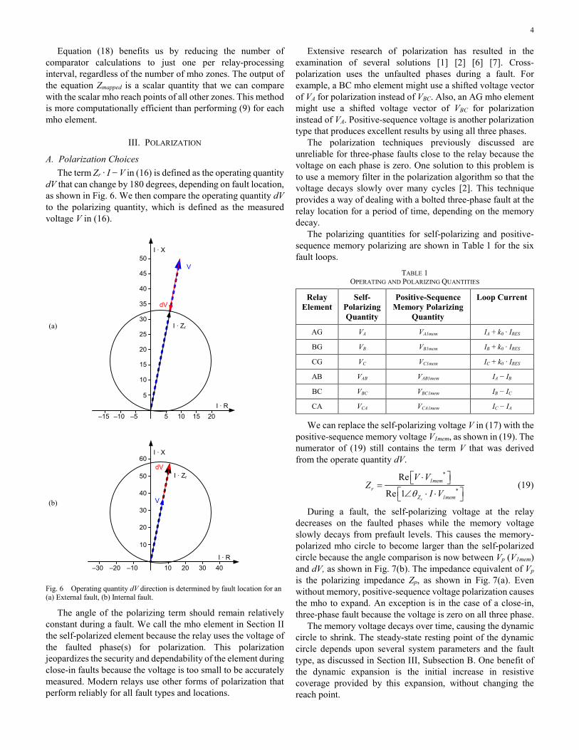
A. Polarization Choices The term Zr ∙ I − V in (16) is defined as the operating quantity

dV that can change by 180 degrees, depending on fault location, as shown in Fig. 6. We then compare the operating quantity dV to the polarizing quantity, which is defined as the measured voltage V in (16).

5

I ∙ X

I ∙ R

V

dV

I ∙ Zr

10

15

20

25

30

35

40

45

50

5 10 15 20–5–10–15

(a)

10

10–10

I ∙ X

I ∙ R

V

dVI ∙ Zr

20

30

40

50

60

–20–30 20 30 40

(b)

Fig. 6 Operating quantity dV direction is determined by fault location for an (a) External fault, (b) Internal fault.

The angle of the polarizing term should remain relatively constant during a fault. We call the mho element in Section II the self-polarized element because the relay uses the voltage of the faulted phase(s) for polarization. This polarization jeopardizes the security and dependability of the element during close-in faults because the voltage is too small to be accurately measured. Modern relays use other forms of polarization that perform reliably for all fault types and locations.

Extensive research of polarization has resulted in the examination of several solutions [1] [2] [6] [7]. Cross-polarization uses the unfaulted phases during a fault. For example, a BC mho element might use a shifted voltage vector of VA for polarization instead of VBC. Also, an AG mho element might use a shifted voltage vector of VBC for polarization instead of VA. Positive-sequence voltage is another polarization type that produces excellent results by using all three phases.

The polarization techniques previously discussed are unreliable for three-phase faults close to the relay because the voltage on each phase is zero. One solution to this problem is to use a memory filter in the polarization algorithm so that the voltage decays slowly over many cycles [2]. This technique provides a way of dealing with a bolted three-phase fault at the relay location for a period of time, depending on the memory decay.

The polarizing quantities for self-polarizing and positive-sequence memory polarizing are shown in Table 1 for the six fault loops.

TABLE 1 OPERATING AND POLARIZING QUANTITIES

Relay Element

Self-Polarizing Quantity

Positive-Sequence Memory Polarizing

Quantity

Loop Current

AG VA VA1mem IA + k0 ∙ IRES

BG VB VB1mem IB + k0 ∙ IRES

CG VC VC1mem IC + k0 ∙ IRES

AB VAB VAB1mem IA − IB

BC VBC VBC1mem IB − IC

CA VCA VCA1mem IC − IA

We can replace the self-polarizing voltage V in (17) with the positive-sequence memory voltage V1mem, as shown in (19). The numerator of (19) still contains the term V that was derived from the operate quantity dV.

*

*

Re

Re 1

⋅ = ∠ ⋅ ⋅ r

1memr

Z 1mem

V VZ

I Vθ (19)

During a fault, the self-polarizing voltage at the relay decreases on the faulted phases while the memory voltage slowly decays from prefault levels. This causes the memory-polarized mho circle to become larger than the self-polarized circle because the angle comparison is now between Vp (V1mem) and dV, as shown in Fig. 7(b). The impedance equivalent of Vp is the polarizing impedance Zp, as shown in Fig. 7(a). Even without memory, positive-sequence voltage polarization causes the mho to expand. An exception is in the case of a close-in, three-phase fault because the voltage is zero on all three phase.

The memory voltage decays over time, causing the dynamic circle to shrink. The steady-state resting point of the dynamic circle depends upon several system parameters and the fault type, as discussed in Section III, Subsection B. One benefit of the dynamic expansion is the initial increase in resistive coverage provided by this expansion, without changing the reach point.

5

3

2

1

1 2–1

X

R

Z

Zr

Zp

–2

dZ

(a)

10

10–10

I ∙ X

I ∙ R

V

I ∙ Zr

Vp

20

30

40

50

60

70

20 30 5040–20–30–40–50–10

dV

(b)

Fig. 7 Dynamic mho characteristic on the (a) Impedance plane, (b) Voltage plane.

Positive-sequence memory polarization may be preferred over cross-polarization because it improves single-pole trip security and has excellent expansion properties [1]. The positive-sequence polarizing and operating quantities for each relay element in Table 1 are shown in Table 2.

TABLE 2 POSITIVE-SEQUENCE MEMORY POLARIZING QUANTITIES*; a = 1∠120°

Polarizing Quantity Polarizing Equation

VA1mem ES − IPrefault ∙ ZS1

VB1mem a2 ∙ VA1mem

VC1mem a ∙ VA1mem

VAB1mem −j ∙ a ∙ VA1mem ∙ 3

VBC1mem −j ∙ VA1mem ∙ 3

VCA1mem −j ∙ a2 ∙ VA1mem ∙ 3

* Based on the system shown in Fig. 1(a); ABC rotation assumed.

From Table 2, we can observe that the prefault current IPrefault affects the positive-sequence voltage at the relay the moment before the fault occurs. Section III, Subsection C explores the effects of load flow.

B. Visualizing Positive-Sequence Polarization We can use a two-source system to analyze a typical relay

response on a transmission line, as shown in Fig. 1(a). The system parameters for the following examples are kept simple in order to aid visual understanding, as shown in Table 3.

TABLE 3 VISUALIZATION SYSTEM PARAMETERS

Parameter Value Unit Description

ZS1 1∠80° Ω (sec) Sending-end positive-sequence source impedance

ZS0 3∠80° Ω (sec) Sending-end zero-sequence source impedance

ZL1 3∠80° Ω (sec) Positive-sequence line impedance

ZL0 9∠80° Ω (sec) Zero-sequence line impedance

ZR1 1∠80° Ω (sec) Receiving-end positive-sequence source impedance

ZR0 3∠80° Ω (sec) Receiving-end zero-sequence source impedance

ES 67∠0° V (sec) Sending-end source voltage

ER 67∠0° V (sec) Receiving-end source voltage

Z1P 3 Ω (sec) Relay reach setting

k0 0.67∠0° unitless Zero-sequence compensation factor

ZFG* 0.5 Ω (sec) Ground fault impedance

ZFP* 0.6 Ω (sec) Phase-to-phase fault impedance

m 0.43 p.u. of ZL

Distance on line to fault

* Where applicable.

The maximum mho expansion occurs at fault inception because V1mem equals the positive-sequence voltage just prior to the disturbance. The memory voltage diminishes over time until it reaches the final value of positive-sequence voltage during the fault. The following subsections describe this expansion and decay for each type of fault.

1) Three-Phase Fault Think of the origin of the impedance plane as the location of

the relay. During a fault on the line, the measured value of the faulted voltage V diminishes, while V1mem initially retains the value it had before the disturbance. On the impedance plane, this means that the magnitude of the measured impedance Z is significantly less than the polarizing impedance Zp, and the dynamic mho circle envelops the origin, as shown in Fig. 8.

6

3

2

1

1 2–1

X

R

Z

dZ

ZS1

Zp

–2 3

Zr

Fig. 8 Dynamic mho characteristic (maximum expansion).

We calculate the polarizing impedance Zp by dividing V1mem by the loop current. If we ignore the effects of load flow, V1mem initially equals the source voltage ES; therefore, in this case, Zp equals the source impedance plus the apparent impedance measured by the relay to the fault Z. This is shown graphically in Fig. 8, where the impedance from the relay location at the origin to the tail of Vector Zp equals Zp − Z = ZS1.

The mho expansion for forward faults depends on the magnitude of the source impedance, a concept known commonly as “expanding back to the source.” The greater the ratio of the source impedance to the line impedance (source-to-impedance ratio, or SIR), the greater the dynamic mho expansion. Note that the maximum expansion back to the source shown in Fig. 8 uses the same system parameters and applies for all types of faults examined in this section, unless otherwise noted.

The memory voltage V1mem eventually decays to the measured positive-sequence voltage V1, which is equal in magnitude to VA, VB, and VC in a balanced system; therefore, the dynamic mho circle for a three-phase fault eventually shrinks to the smaller self-polarized circle, as shown in Fig. 9. The voltage and current vectors for this diagram are shown in Fig. 10. Fig. 11 shows the substantial voltage decay over time for a three-phase fault.

3

2

1

1 2–1

X

R

Z

dZ

Zr

Zp

Fig. 9 Three-phase fault dynamic mho characteristic (steady state). Vectors Z and Zp overlap.

40–40

IA

VA

ICIB

VC

VB–40

40

Fig. 10 Three-phase fault vectors for voltage and current.

40–40

VA1mem

VC1mem

VB1mem –40

40

–60

–60

60

60

Fig. 11 Three-phase fault relay vectors; dashed lines represent expanded memory voltage vectors, and solid lines represent steady state.

Based on [3], the expansion is derived mathematically as a vector that begins at the origin and ends at the dynamic mho circle. This vector is represented as b for the steady-state mho characteristic, and bmem for the full expansion. For a three-phase fault, we have (20).

0== −mem S1

bb Z

(20)

7

3

2

1

1 2–1

X

R

b(mem)

Zr

–2

Fig. 12 Vector bmem representation of expansion and steady state.

In this example, bmem, shown in Fig. 12, has a magnitude of ZS1. When the memory voltage reaches steady state, b is at a distance of zero from the origin, which means that the dynamic circle and the self-polarized (or “static” circle) overlap.

2) Phase-to-Phase Fault The dynamic mho for a phase-to-phase fault initially

expands back to the source (as explained in Section III, Subsection B) and eventually decays to 0.5 ∙ ZS1, as proved by Calero [3]. We can express the dynamic expansion vector as shown in (21).

2= −

= −

S1

mem S1

Zb

b Z (21)

The dynamic mho does not shrink to the self-polarized mho circle, no matter how much time elapses, as shown in Fig. 13. This is logical because the polarizing memory voltage VBC1mem at steady-state fault current exceeds the measured quantity VB − VC (see Table 2). On the impedance plane, this means that the polarizing impedance Zp always exceeds the measured loop impedance Z. The voltage and current vectors for the phase-to-phase fault are shown in Fig. 14. The memory voltage decay for a phase-to-phase fault is less than that for a three-phase fault, as shown in Fig. 15.

The expansion properties of the dynamic mho circle during phase-to-phase faults are simple, for two reasons. First, the derivation does not involve the zero-sequence network and so does not contain zero-sequence impedances. Second, negative-sequence impedances are often assumed to equal corresponding positive-sequence impedances.

3

2

1

2–1

X

R

Z

0.5 ∙ ZS1

Zp

–2

dZ

–1

1

Zr

Fig. 13 Phase-to-phase fault dynamic mho characteristic (steady state).

40–40

IC VA

IB

VC

VB–40

40

60

Fig. 14 BC fault vectors for voltage and current.

40–40

VA1mem

VC1mem

VB1mem

40

60

60

80

–60

–40

20–20

Fig. 15 BC fault relay vectors; dashed lines represent expanded memory voltage vectors, and solid lines represent steady state.

3) Phase-to-Phase-to-Ground Fault As with other faults we have examined up to this point, the

dynamic mho expansion during a phase-to-phase-to-ground fault depends on the source impedance ZS1. The dynamic mho characteristic decays to a value given by (22), as proved by Calero [3].

2 2 + ⋅

= − + ⋅ + ⋅ + ⋅ ⋅ = −

S0 L0S1

S1 L1 S0 L0

mem S1

Z m Zb Z

Z m Z Z m Zb Z

(22)

8

The derivation of non-memory Vector b is significantly more complicated than for three-phase or phase-to-phase faults. The expansion depends on the zero-sequence network as well as on the impedance of the line to the fault in per unit m. The maximum decay, shown in (22), will be less than 0.5 ∙ ZS1, as shown in Fig. 16. The voltage and current vectors for this fault are shown in Fig. 17. The memory voltage decay, shown in Fig. 18, is similar to a phase-to-phase fault.

3

2

1

2–1

X

R

Z

0.43 ∙ ZS1

Zp

–2

dZ

–1

1

Zr

Fig. 16 Phase-to-phase-to-ground fault dynamic mho characteristic (steady state).

40–40

IB VAIC

VC

VB –40

40

6020–20

Fig. 17 BCG fault vectors for voltage and current.

40–40

VA1mem

VC1mem

VB1mem

40

60

60

–60

–40

–20 20

Fig. 18 BCG fault relay vectors; dashed lines represent expanded memory voltage vectors, and solid lines represent steady state.

4) Phase-to-Ground Fault The expansion of the phase-to-ground dynamic mho is

influenced by the current compensation factor k0 [6]. The expansion vectors are shown in (23) [3].

1

1

2

2

2

+ = − +

+ = − +

S0

S1S1

L0

L1

S0

S1mem S

L0

L1

ZZ

b Z ZZ

ZZ

b Z ZZ

(23)

The maximum expansion described by bmem in (23) has a magnitude of ZS1 in systems where the angles and ratios of ZS0, ZS1 and ZL0, ZL1 are equal. The expansion shrinks to 0.80 ∙ ZS1, as shown in Fig. 19, using the system parameters in Table 3. The dynamic characteristic for a phase-to-ground fault provides the benefit of increased resistive fault coverage, which is often crucial during ground faults. The voltage and current vectors for this fault are shown in Fig. 20. The memory voltage decay for a phase-to-ground fault is shown in Fig. 21. The steady-state positive-sequence voltage remains strong because of the two healthy phase voltages.

3

2

1

2

X

R

Z

0.8 ∙ ZS1

Zp

–2

dZ

–1

1

Zr

Fig. 19 Phase-to-ground fault dynamic mho characteristic (steady state).

9

40–40IA

VA

VC

VB

–40

40

20–20

–60

60

–60

Fig. 20 BCG fault vectors for voltage and current.

40–40

VA1mem

VC1mem

VB1mem

40

60

60

–60

–40

–20 20

Fig. 21 AG fault relay vectors; dashed lines represent expanded memory voltage vectors (not visible in this figure because the vectors are too short), and solid lines represent steady state.

5) Reverse Fault We can simulate a reverse fault by shifting the fault current

phasors by 180 degrees; the voltage change is negligible for a close-in fault on either side of the current transformers (CTs). For a close-in reverse fault in Fig. 1(a), the relay measures fault current supplied by the remote source ER. The relay source impedance is now in front of the relay, with respect to the fault location, and equal to ZL1 + ZR1.

The source impedance begins in the first quadrant on the impedance plane and ends at the origin for an inductive system, as shown in Fig. 22. This represents the impedance from the remote source to the relay location. Adding a small amount of fault resistance separates the vectors and allows them to be seen more clearly.

3

2

–1

X

R

Z

Zp

–2

dZ

ZL1 + ZR1

4

1 2

Zr(a)

3

2

–1

X

R

Z

Zp

–2

dZ

0.8 ∙ (ZL1 + ZR1)

1 2

Zr

(b)

Fig. 22 Close-in reverse phase-to-ground fault dynamic mho characteristic with arc resistance added: (a) Maximum expansion, (b) Steady state. Note that the dynamic mho (dashed circle) determines operation. The self-polarized mho (solid circle) is shown as a reference.

Several impedance vectors change direction for a reverse fault, causing the dynamic mho to shrink. Vectors Z and Zp reverse directions for faults behind the relay; Zr is constant in the relay defined by the reach setting, and it continues to point in the forward direction. The polarizing impedance Zp points from the location of the source to the measured impedance Z. Because the dynamic mho is defined between the tail of Zp and the tip of dZ, the dynamic circle becomes smaller than the self-polarized mho under this condition.

A smaller operating characteristic during reverse faults alleviates some directional security concerns regarding the mho expansion. In Fig. 22(b), the distance between the origin and the tail of Vector Zp initially equals | ZL1 + ZR1 |. At steady state, Zp shrinks to 80 percent of its original value, Fig. 22(b), using the parameters in Table 3. Over time, the decay in the polarizing quantity is analogous to the forward AG event described under “Phase-to-Ground Fault” in Section III, Subsection B. We can apply similar logic to other reverse fault types.

10

C. Load Flow In a two-machine lossless system, such as in Fig. 1(a), with

no fault, we can represent the power sent over the transmission line by the power-flow equation shown in (24).

( ),sin⋅

= S R S R1,2

total

E EP

Xδ

(24)

where

( ) ( ), arg arg= −S R S RE Eδ (25)

Xtotal is the total reactance between sources ES and ER. Power flows from the source with the leading voltage angle, and this creates a positive-sequence voltage drop across the source impedance; therefore, the positive-sequence memory voltage at the relay is unequal to the source voltage at fault inception. The memory voltage phase angle may shift, changing the position of the polarizing impedance Zp.

The voltage drop across the source impedance is relatively small during prefault conditions when compared to a bolted fault. We simulate this in Fig. 23, which shows a three-phase fault placed on a homogeneous system with positive power flow and no fault resistance. VA1mem represents the prefault (memory) voltage, and VA is the measured fault voltage on A-phase.

Im(V)

Re(V)

ES

dVAVA

20 40 60

20

40

(a)

Im(V)

Re(V)

ES ES − Ipf ∙ ZS1

VA1mem

20 40 60

20

40

(b)

Im(V)

Re(V)

VA

20 40 60

20

40

VA1mem

(c)

Fig. 23 Voltage vectors during a three-phase fault with prefault current (positive power flow) on a homogeneous system with no fault resistance; compare (a) ES with VA, (b) ES with VA1mem, (c) VA with VA1mem.

If we define Ifault as the fault loop current, we calculate the two impedance vectors as shown in (26) and (27).

= 1memp

fault

VZ

I (26)

= A

fault

VZ

I (27)

If we extend the logic of (26) and (27) to all forward faults, Vectors Zp and Z are separated by angle θ, as shown in Fig. 24. For example, during an AG fault, θ represents the phase shift between VA and VA1mem. Over time, θ decreases as the memory voltage decays.

3

2

1

2

X

R

Z

Zr

Zp

–2

dZ

–1

θ

Fig. 24 Positive load flow reducing resistive fault coverage by shifting the dynamic mho to the left.

11

Vector VA1mem, and therefore Zp, increasingly lags the measured fault voltage VA for forward power flow as the prefault current increases. This causes Zp to shift the dynamic mho circle to the left for forward load flow; reverse load flow has the opposite effect. Four impedance graphs in Fig. 25 illustrate this effect for different levels of load flow.

2

1

2

X

R

Z

Zr

Zp

–2

dZ

1

3

2

1

2

X

R

Z

Zr

Zp

–2

dZ

1

3

2

1

2

X

R

Z

Zr

Zp

–2

dZ

1

3

2

1

2

X

R

Z

Zr

Zp

–2

dZ

1

3

(a) (b)

(c) (d)

Fig. 25 Dynamic mho during fault conditions with varying sending source angle: (a) −40°, (b) −20°, (c) 0°, (d) 20°.

Distance-element overreach for high-resistance faults during heavy forward/reverse load conditions is a concern when applying distance elements. The adaptability of the positive-sequence memory-polarized distance element minimizes overreaching concerns [11].

IV. TESTING

A. Justification for Testing Dynamic mho expansion varies based on manufacturer

implementation of the elements. In one implementation, the time constant of the memory polarization is four cycles [2].

We advise testing the dynamic mho when assessing the performance of the element on lines with series capacitors. The dynamic mho expansion is necessary to detect forward faults that are directly in front of a line-end capacitor with bus-side potential transformers (PTs) (see Section V, Subsection B). Often, this type of testing employs a real-time simulator, where the relay is included in the playback loop.

In practice, the static or self-polarized mho is tested extensively at steady state; for most applications, the reach point is the most important aspect of the element. We recommend testing mho elements by using values from a constant-source impedance model.

B. Testing Considerations Section III shows that the dynamic circle does not shrink

back to the self-mho circle except in the case of a three-phase fault. This may be confusing to a relay tester using a common test procedure because the mho element appears to operate as if the dynamic circle did not exist.

The dynamic mho element does not usually interfere with testing because of the test voltages that are typically used. Table 4 lists several test voltages and currents used to test a phase-to-ground mho circle by simulating an AG fault.

TABLE 4 EXAMPLE TEST QUANTITIES

Test Quantity

Test 1 Test 2 Test 3 Test 4

VA V (sec) 27∠0° 27∠0° 27∠20° 27∠−20°

VB V (sec) 67∠−120° 67∠−120° 67∠−120° 67∠−120°

VC V (sec) 67∠120° 67∠120° 67∠120° 67∠120°

V1 V (sec) 53.67∠0° 53.67∠0° 53.21∠3.3° 53.21∠−3.3°

IA A (sec) 3∠−20° 1.6∠−60° 2.64∠−20° 3.19∠−20°

Note: IB = IC = 0 A.

The voltage angles in Tests 1 and 2 for VA, VB, and VC are, respectively, 0, −120, and 120 degrees. This means that voltage VA is in phase with V1mem; therefore, the impedance vector Z is in phase with Zp.

For an AG fault,

=+ ⋅

A

A 0 R

VZ

I k I (28)

=+ ⋅

1memp

A 0 R

VZ

I k I (29)

where IR represents the residual current, or sum of the phase current (IA + IB + IC). Vectors Z and Zp overlap because they are in phase; therefore, the angle difference between Zp and dZ is 90 degrees when the measured impedance is on the self-polarized mho circle.

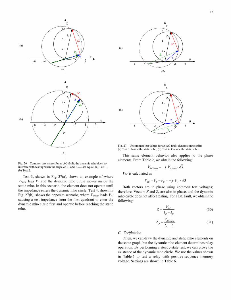
The graphical results shown in Fig. 26 for Tests 1 and 2 show that, in testing this way, the dynamic mho circle asserts at the same time as the self-polarized mho circle. With proper test voltages, the user does not see the effects of the dynamic mho circle.

12

6

4

2

4

X

RZ

Zr

Zp

–4

dZ

–2

–6

(a)

6

4

2

6–2

X

R

ZZr

Zp

–4

dZ

–2

–6 2 4

–4

–6

(b)

Fig. 26 Common test values for an AG fault; the dynamic mho does not interfere with testing when the angle of VA and V1mem are equal: (a) Test 1, (b) Test 2.

Test 3, shown in Fig. 27(a), shows an example of where V1mem lags VA and the dynamic mho circle moves inside the static mho. In this scenario, the element does not operate until the impedance enters the dynamic mho circle. Test 4, shown in Fig. 27(b), shows the opposite scenario, where V1mem leads VA, causing a test impedance from the first quadrant to enter the dynamic mho circle first and operate before reaching the static mho.

6

4

2

X

RZ

Zr

Zp

–4

dZ

–2

–6 2 4

(a)

6

4

2

X

RZ

Zr

Zp

–4

dZ

–2–6 2 4

(b)

Fig. 27 Uncommon test values for an AG fault; dynamic mho shifts (a) Test 3: Inside the static mho, (b) Test 4: Outside the static mho.

This same element behavior also applies to the phase elements. From Table 2, we obtain the following:

3= − ⋅ ⋅BC1mem A1memV j V

VBC is calculated as

3= − = − ⋅ ⋅BC B C A1V V V j V

Both vectors are in phase using common test voltages; therefore, Vectors Z and Zp are also in phase, and the dynamic mho circle does not affect testing. For a BC fault, we obtain the following:

=−BC

B C

VZ

I I (30)

=−

BC1memp

B C

VZ

I I (31)

C. Verification Often, we can draw the dynamic and static mho elements on

the same graph, but the dynamic mho element determines relay operation. By performing a steady-state test, we can prove the existence of the dynamic mho circle. We use the values shown in Table 5 to test a relay with positive-sequence memory voltage. Settings are shown in Table 6.

13

TABLE 5 VERIFICATION TEST QUANTITIES

Test Parameter Applied Voltage Unit (Sec)

VA 35∠40° V

VB 40∠−100° V

VC 45∠160° V

V1 39.86∠13.3° V

TABLE 6 VERIFICATION RELAY SETTINGS

Relay Setting Value Unit

Zone 1 reach 6.24 Ω (sec)

Line impedance 7.8 Ω (sec)

Line angle 84 Degrees

| k0 | 0.726 unitless

arg (k0) –3.69 Degrees

We set the current test angle to 0 degrees and vary the magnitude. Maintaining constant voltage and slowly increasing the current ensures that the dynamic mho has minimal expansion. The position of the static and dynamic mho circles are shown in Fig. 28. The locus of impedance test points Ztest_locus shows the impedance trajectory as the test current increases from 4.41 to 4.93 A (sec).

4

2

X

R

| IA | = 4.41 AZr

–4

Ztest_locus

–2 2 4

| IA | = 4.93 A

Fig. 28 Uncommon test values interfere with mho element testing.

As the current magnitude increases, the dynamic circle moves slightly in real-time. It is clear that the apparent impedance test point does not intersect both mho circles at the same point. Without a knowledge of the dynamic mho expansion, a relay tester may expect ground mho operation when | IA | = 4.41 A (sec) because this is the location at which the apparent impedance intersects with the static mho characteristic. In reality, the current needs to increase until the impedance enters the dynamic mho circle at | IA | = 4.93 A (sec) before the element operates.

The dynamic mho circle rarely interferes with testing unless the positive-sequence voltage angle differs from the faulted-phase voltage angle. The relay test voltages in the previous example could be manipulated to force the apparent impedance to intersect the dynamic mho circle before the static mho. In this case, the ground mho element operates before the expected trip current.

V. PRACTICAL CONSIDERATIONS

A. Benefits of Positive-Sequence Memory Voltage There are few settings related to the mho element that a user

must set. The most important of these include the reach point, direction, and line angle or maximum torque angle (MTA). High-impedance fault coverage can be very limited for a self-polarized mho element because the circle does not expand. We can improve resistive coverage by increasing the reach point or varying the MTA, but this is unacceptable in most circumstances.

Positive-sequence memory polarization provides excellent dynamic expansion with good open-pole security compared to other polarizing types, such as self-polarization, cross-polarization, and hybrid polarization [1]. A larger dynamic expansion provides the benefit of additional resistive coverage, without sacrificing security or requiring any settings changes. The expansion properties depend on several factors, including, but not limited to, source and line parameters, load flow, fault type, fault resistance, mho implementation, and memory properties.

Positive-sequence memory voltage has the added benefit of providing proper polarization for faults on any phase and during single-pole tripping applications [1]. During single-pole open intervals, the positive-sequence memory voltage polarization quantity remains stable enough for use with phase- and ground-mho elements.

The sequence network for a single-pole open on a line is shown in Fig. 29. We assume each source contains a zero-sequence source. The positive-sequence current is split between the parallel branches of negative- and zero-sequence impedance. The positive-sequence voltage developed at the relay during steady state is less than nominal three-phase voltage, but it is still sufficient for polarization.

ZS1 mZL1 (1 – m)ZL1 ZR1

ES ER

ZS2 mZL2 (1 – m)ZL2 ZR2

ZS0 mZL0 (1 – m)ZL0 ZR0

Fig. 29 Sequence networks with single-pole open.

By contrast, ground quadrilateral elements provide user-settable resistance blinder thresholds for greater control of fault resistance coverage; however, these elements often use negative- or zero-sequence current for polarization and must be disabled during single-pole open applications [5].

14

B. Expansion and Security Mho elements are inherently directional, as shown in Fig. 8

and Fig. 22. Forward faults expand the dynamic element back towards the source, and reverse faults shrink the element in the first quadrant.

As with the use of other elements, there are some instances where using the mho element poses a security concern. An example would be for ground-distance element overreach during phase-to-phase-to-ground faults [1]. We can largely mitigate these security concerns by supervising the mho characteristic with directional and fault-identification logic [4].

In such a special case as a series capacitor application, we strongly recommend transient simulations to ensure proper dynamic operation. The capacitive impedance in these scenarios can place more emphasis on dynamic expansion for proper relay operation. For example, in Fig. 30 we apply a three-phase fault close to relays R1 and R2, which have positive-sequence memory polarization.

ES ER

ZS1

Xc

ZL1 ZR1

3ph

R2 R1

Fig. 30 Relays R1 and R2 with bus-side PTs react to a three-phase fault beyond a series capacitor on a local line.

The impedance Z measured by R1 will be close to −90 degrees, as shown in Fig. 31, and the dynamic expansion is crucial to proper relay operation. Several system parameters affect relay operation. These parameters include the magnitude of the capacitive reactance, the extent of the dynamic expansion, and filtering delays. The element initially operates if | ZS1 | < | Xc | and eventually restrains as the dynamic circle shrinks to the self-polarized element.

3

2

1

2–1

X

R

Z

Zr

Zp

–2

dZ

1

Fig. 31 Impedance diagram for Relay R1 in response to a forward three-phase fault on the opposite side of the series capacitor.

Relay R2 initially restrains for the three-phase reverse fault but may eventually operate as the dynamic mho shrinks back to the self-polarized mho. A properly set directional element that supervises the mho element prevents relay operation even if the impedance plots inside the dynamic mho circle. The progression of the dynamic characteristic is shown in Fig. 32(a). If the fault is not three-phase, the dynamic mho will not completely shrink to the self-polarized mho, as described in Section III. In most cases, the reach point Zr exceeds the series capacitor reactance Xc; however, if the opposite is true, then R2 will operate during mho expansion and restrain during steady state, as shown in Fig. 32(b).

3

2

2–1

X

R

Z

Zr

Zp

–2

dZ

1

4

100%50%0%

Percent Expansion

1 ∙ ZS1

(a)

0.2

0.4–0.2

X

R

Z

Zr

Zp

–0.4

dZ

0.2

100%

Percent Expansion1 ∙ ZS1

(b)

1

80%

60%

40%

20%

0%

Fig. 32 Impedance diagram for Relay R2 in response to a reverse three-phase fault on the opposite side of the series capacitor: (a) Case I: | Zr | > | Xc |, (b) Case II: | Zr | < | Xc |.

These examples highlight the importance of transient testing with series-compensated lines. Real-world cases can be significantly more involved when we consider other factors such as parallel-compensated lines, bus versus line PTs, midline versus end compensation, and subharmonic transients [8].

15

VI. CONCLUSION Dynamic mho elements with positive-sequence memory

polarization have large expansion and excellent single-pole open security. This expansion provides additional resistive coverage during faults, directional security, and protection for close-in faults. The time-varying nature of the element can be visualized with vectors on the impedance plane.

The dynamic mho behavior is affected by system parameters, load flow, fault type, and the relay algorithm. Real-time transient simulations are recommended for applications such as series-compensated lines, where the dynamic mho element is expected to play a crucial role in relay operation.

A thorough understanding of the distance-element concepts presented in this paper is intended to help in the following ways:

• Relay testers can avoid misinterpreting results when performing transient and steady-state tests.

• Disturbance-analysis teams can assess the performance of a mho element based on changing system conditions.

• Users creating settings can better understand system conditions that adversely affect mho performance.

VII. REFERENCES [1] E. O. Schweitzer, III and J. Roberts, “Distance Relay Element Design,”

Proceedings of the 46th Annual Conference for Protective Relay Engineers, College Station, TX, April 1993.

[2] E. O. Schweitzer, III, “New Developments in Distance Relay Polarization and Fault Type Selection,” presented at the 16th Annual Western Protective Relay Conference, Spokane, WA, October 1989.

[3] F. Calero, “Distance Elements: Linking Theory With Testing,” 62nd Annual Conference for Protective Relay Engineers, Austin, TX, April 2009, pp. 333–352.

[4] D. Costello, “Determining the Faulted Phase,” 63rd Annual Conference for Protective Relay Engineers, College Station, TX, April 2010, pp. 1–20.

[5] H. Altuve Ferrer and E. O. Schweitzer, III, “Modern Solutions for Protection, Control, and Monitoring of Electric Power Systems,” Schweitzer Engineering Laboratories, Inc., Pullman, WA, 2010.

[6] S. Zocholl, “Three-Phase Circuit Analysis and the Mysterious k0 Factor,” 22nd Annual Western Protective Relay Conference, Spokane, WA, October 1995.

[7] L. M. Wedepohl, “Polarized Mho Distance Relay,” Proceedings of IEE, Volume 112, No. 3, March 1965.

[8] H. Altuve, J. Mooney, G. Alexander, “Advances in Series-Compensated Line Protection,” 35th Annual Western Protective Relay Conference, Spokane, WA, October 2008.

[9] J. Zydanowicz, “Application of the Idea of Steady-State Impedance and Admittance to the Construction of Diagrams Intended for the Analysis of the Operation of Distance and Directional Relays and Protective Schemes,” Conférence Internationale des Grands Reseaux Électriques à Haute Tension, Paris, France, June 1960.

[10] L. P. Cavero, “Analysis of Complex Distance-Relay Characteristics Taking Load Into Account,” IEE Conf. Publ. 185, 1980, pp. 192–194.

[11] J. Roberts, A. Guzman, and E. O. Schweitzer III, “Z=V/I Does Not Make a Distance Relay,” presented at the 20th Annual Western Protective Relay Conference, Spokane, WA, October 1993.

VIII. BIOGRAPHY Donald D. Fentie received his B.Sc. degrees in Electrical Engineering and Computer Science in 2006 and his M.Sc. degree in Electrical Engineering in 2010 from the University of Saskatchewan. Mr. Fentie worked as a protection engineer and field engineer for Magna Electric Corporation in Saskatoon, Saskatchewan from 2006 to 2010. He joined Schweitzer Engineering Laboratories, Inc. (SEL) in 2010 and is currently an application protection engineer in Calgary, Alberta. He is an IEEE member and is registered as a Professional Engineer (P.Eng.) in the province of Alberta.

Previously presented at the 2016 Texas A&M Conference for Protective Relay Engineers.

© 2016 IEEE – All rights reserved. 20160815 • TP6719