Understanding Price Variation in AgriculturalCommodities in India

Shoumitro Chatterjee, Princeton and Devesh Kapur, UPenn

India Policy Forum, July 2016

0-0

Avg Standard Deviation of log real pricesWheat & Paddy in 16 Largest States

0-1

Why should we care?

Important for development of India.

Consumers pay different prices in different regions.

Farmers in different locations face different prices.

They make crop choices and input choices given these prices.

Important to understand farm productivity and farmer welfare.

0-2

Outline

Creation of new Agriculture Markets.

Decomposition of Variance

Conceptual Framework

MSP and Government Procurement

Mandis and Market Power

Future Work and Policy Questions

0-3

Acts Governing Agriculture Trade in India.

Food Adulteration Act, 1954

Essential Commodities Act, 1955

Standards of Weights & Measurement Act, 1976

Prevention of Black Marketing & Maintenance of Supply ofEssential Commodities Act, 1980

Consumer Protection Act, 1986

Bureau of Indian Standards Act, 1986

Agriculture Produce (Grading & Marketing) Act, 1986

0-4

Fraction of Mandis Constructed by year

0-5

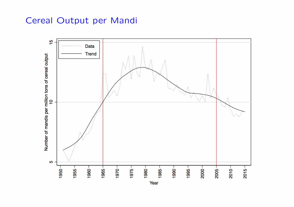
Cereal Output per Mandi

0-6

Variance Decomposition (Shapley Shorrocks)

37%: District Specific Time Invariant effects.

Market Structure, Access to Irrigation, Productivity

20%: Location invariant aggregate time shocks.

Global Demand

4%: Rainfall Shocks

39%: Location and Time varying factors.

Connectivity and Procurement of Grains

0-7

Variance Decomposition (Shapley Shorrocks)

37%: District Specific Time Invariant effects.

Market Structure, Access to Irrigation, Productivity

20%: Location invariant aggregate time shocks.

Global Demand

4%: Rainfall Shocks

39%: Location and Time varying factors.

Connectivity and Procurement of Grains.

0-8

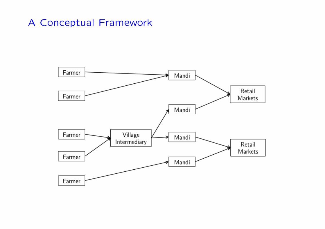
A Conceptual Framework

0-9

A Conceptual Framework

0-10

Data Sources

Time period 2005-2014. Commodities – Paddy & Wheat.

Monthly Wholesale price and quantity data. (Govt. of India’sAgmarknet Project).

Seasonal yields and production data at the district level. (Min-istry of Agriculture, GOI)

Monthly Rainfall - gridded data from Willmott and Matsuura(2012).

Population at sub-district level from Census of India 2011.

Farmer level data from NSS - Situation Assessment of Agricul-tural Households 2012-13.

District level monthly grain procurement - Food Corporation ofIndia.

0-11

Govt Procurement of Paddy and Wheat

Through Food Corporation of India and State Agencies

“Government policy of procurement of Food grains has broadobjectives of ensuring MSP to the farmers” – FCI Website.

Extensive Operations with about 20000 centers for Wheat and40000 centers for Paddy.

What does the data tell us?

0-12

Procurement varies widely in space

0-13

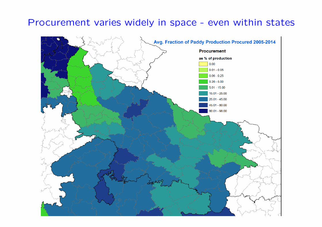
Procurement varies widely in space - even within states

0-14

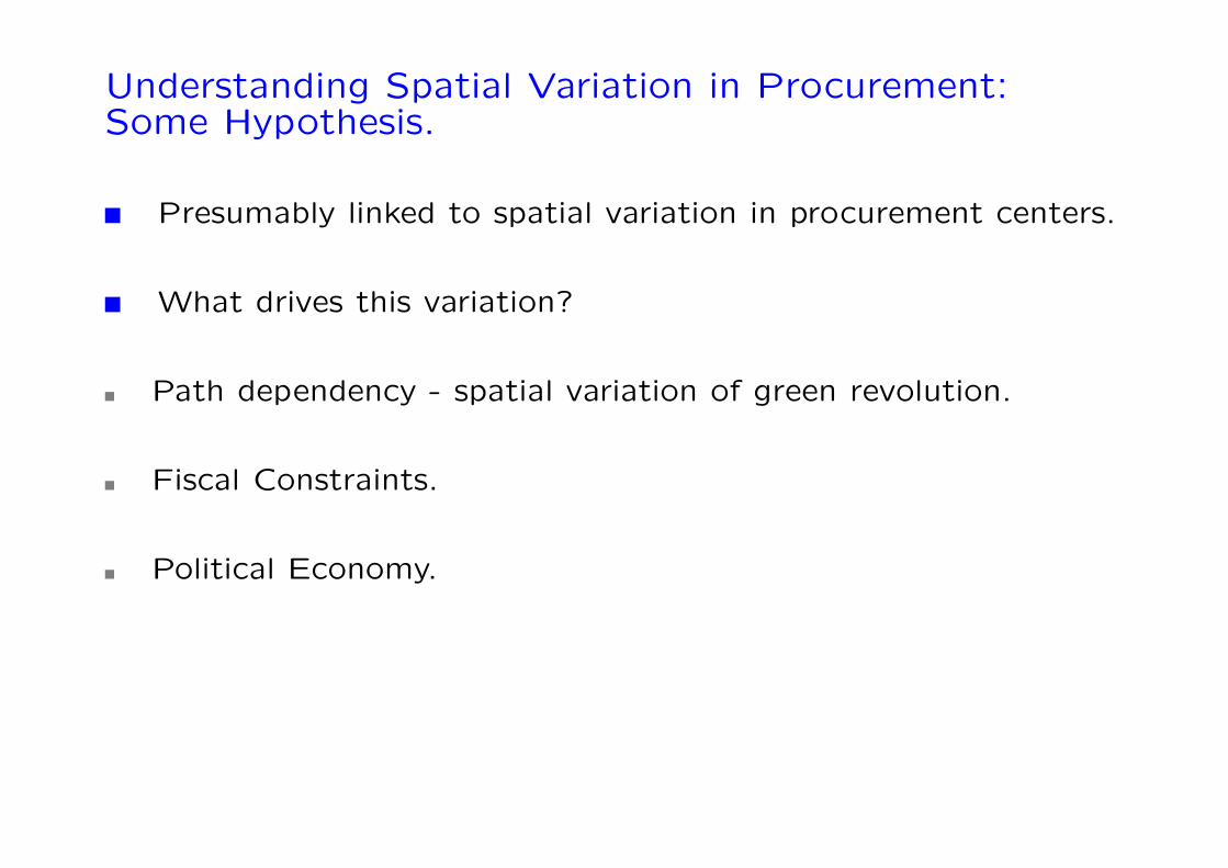
Understanding Spatial Variation in Procurement:Some Hypothesis.

Presumably linked to spatial variation in procurement centers.

What drives this variation?

Path dependency - spatial variation of green revolution.

Fiscal Constraints.

Political Economy.

0-15

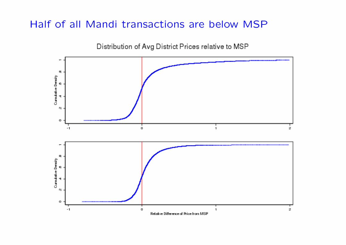
Half of all Mandi transactions are below MSP

0-16

What is the effect on market prices?

(pcdt −mspct

mspct

)= α+ β1 {procurementcdt > 0}+ γd + γt + εcdt

0-17

Local market power of Mandis

0-18

Spatial Distribution of APMC Markets - Andhra Pradesh

0-19

Spatial Distribution of APMC Markets - Uttar Pradesh

0-20

Summary Statistics - Spatial Distribution of Markets

0-21

Summary Statistics - Spatial Distribution of Markets

0-22

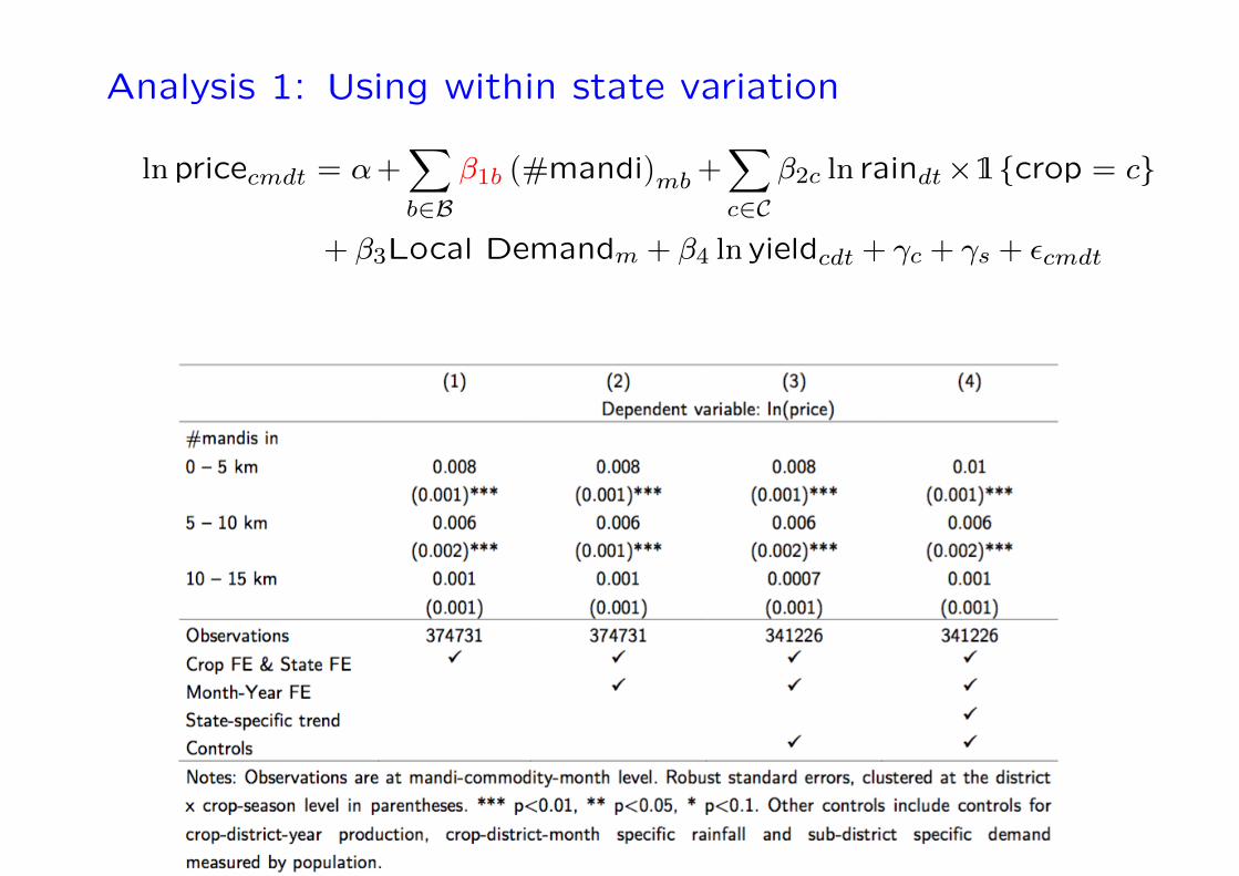
Analysis 1: Using within state variation

lnpricecmdt = α+∑b∈B

β1b (#mandi)mb+∑c∈C

β2c ln raindt×1 {crop = c}

+ β3Local Demandm + β4 ln yieldcdt + γc + γs + εcmdt

0-23

Analysis 2: Matching near state borders - An Illustration

0-24

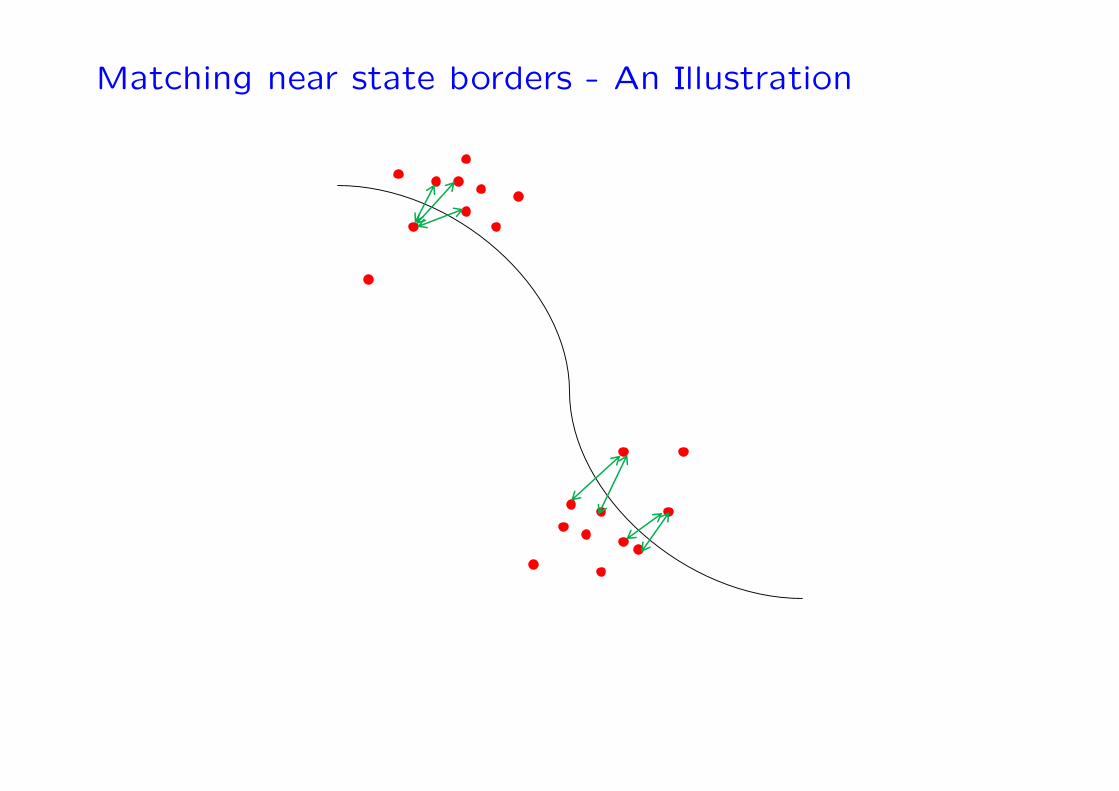
Matching near state borders - An Illustration

0-25

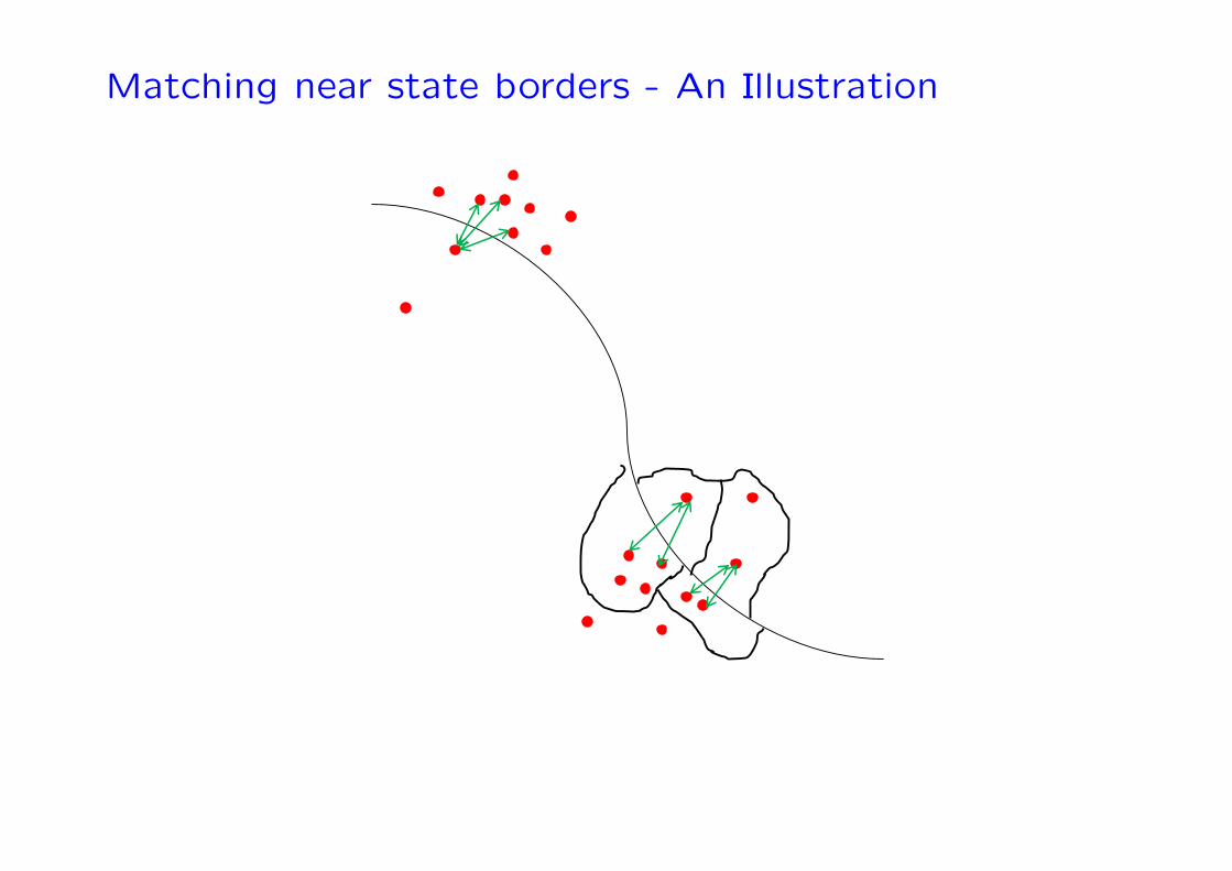
Matching near state borders - An Illustration

0-26

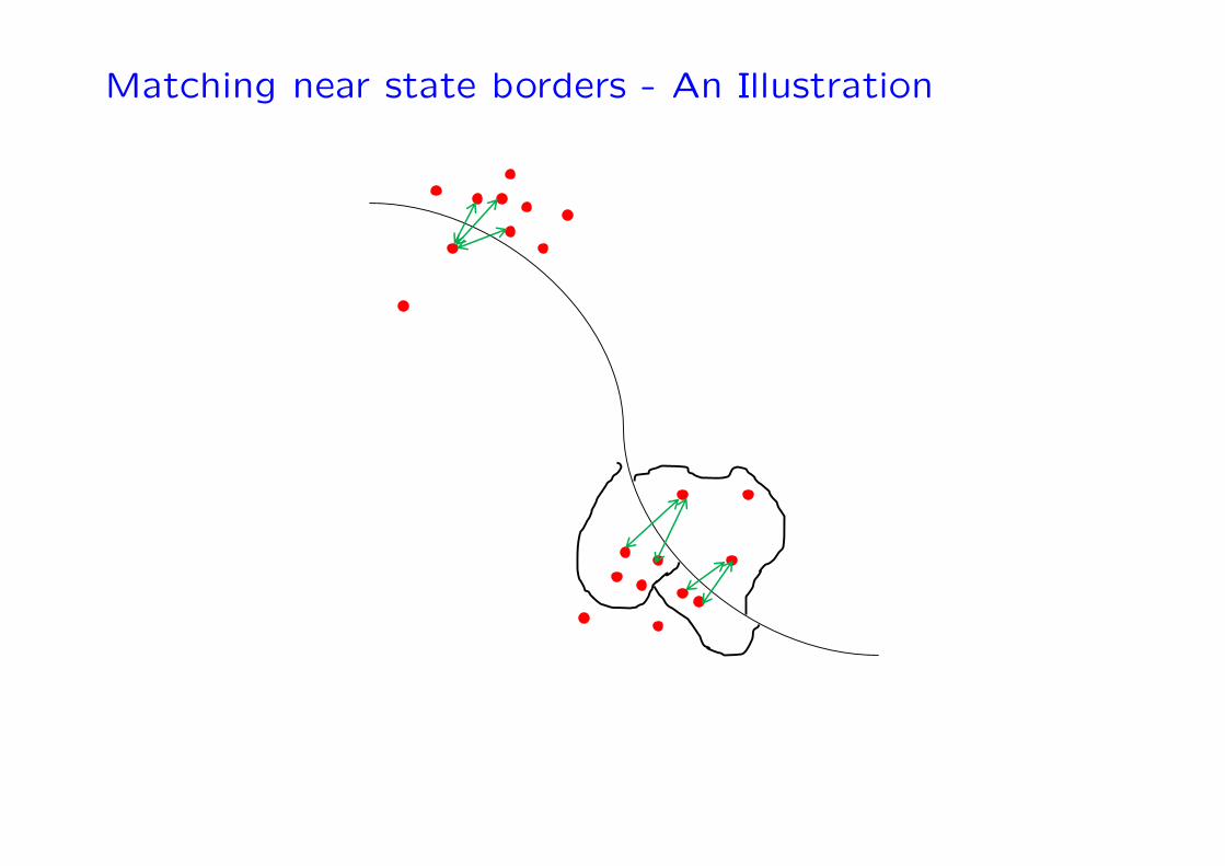
Matching near state borders - An Illustration

0-27

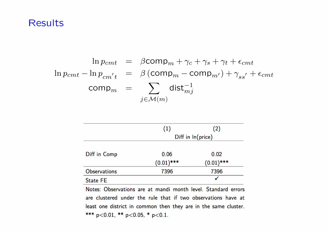
Results

ln pcmt = βcompm + γc + γs + γt + εcmt

ln pcmt − ln pcm′t = β (compm − compm′) + γss′ + εcmt

compm =∑

j∈M(m)

dist−1mj

0-28

Conclusions & Policy Questions

Core objective of MSP is not being met.

Large spatial variation in procurement and is likely to have sig-nificant welfare and distributional consequences.

Policy goal should be to provide more options to the farmers.

Regulations in APMC acts have created market power for man-dis which has clear price effects.

0-29

Conclusions & Policy Questions

Reforms under Model APMC Act –

Levies taxes on transactions outside the mandis.

Some states went back on reforms.

Has failed to attract private players.

NAM – welcome change but effects remain to be seen.

0-30

Stylized Fact#1: Farmer’s Awareness of MSP.Limited and Highly Varying.

0-31

Stylized Fact#2: MSP Awareness vs intensity of pro-curement

0-32

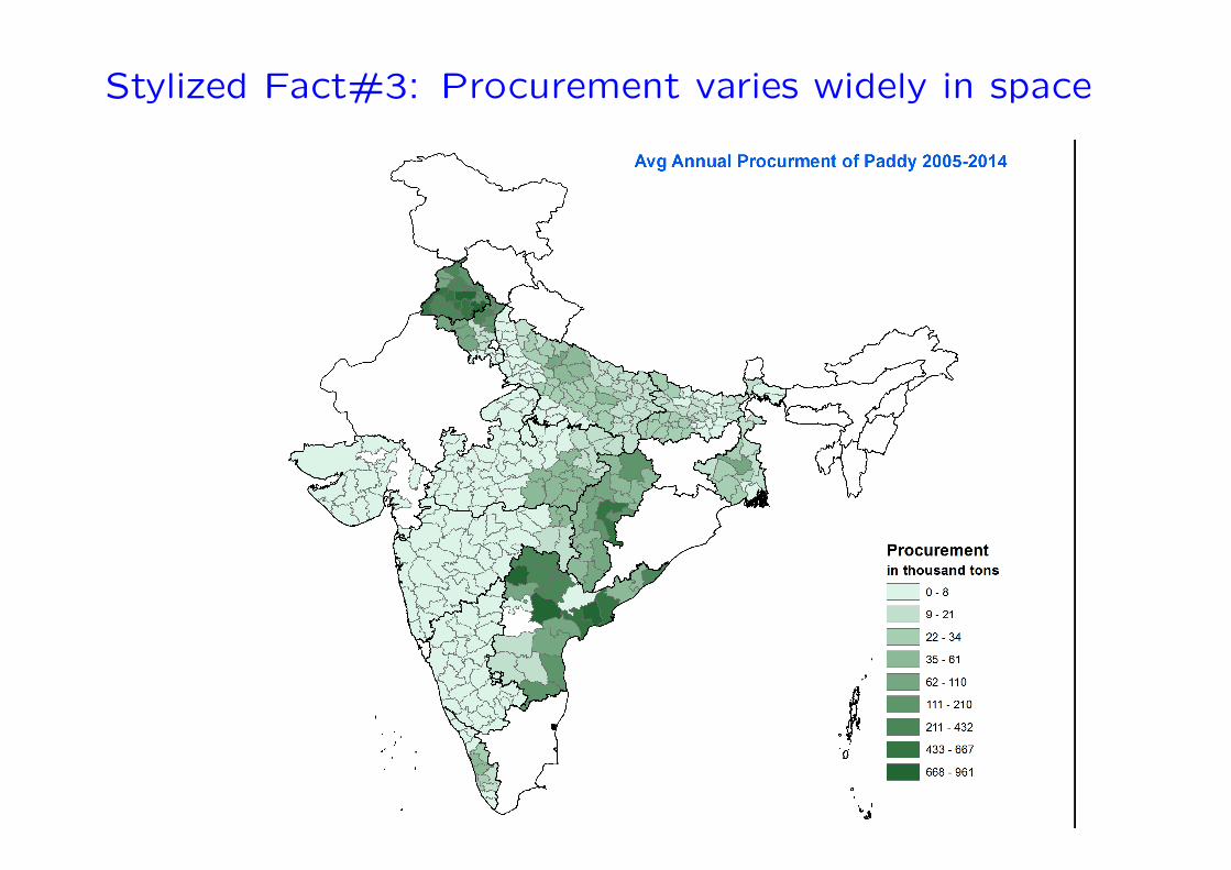
Stylized Fact#3: Procurement varies widely in space

0-33