understanding predictive information criteria for...
TRANSCRIPT
Understanding predictive information criteria for Bayesian models∗
Andrew Gelman†, Jessica Hwang‡, and Aki Vehtari§
14 Aug 2013
Abstract
We review the Akaike, deviance, and Watanabe-Akaike information criteria from a Bayesianperspective, where the goal is to estimate expected out-of-sample-prediction error using a bias-corrected adjustment of within-sample error. We focus on the choices involved in setting up thesemeasures, and we compare them in three simple examples, one theoretical and two applied. Thecontribution of this review is to put all these information criteria into a Bayesian predictivecontext and to better understand, through small examples, how these methods can apply inpractice.
Keywords: AIC, DIC, WAIC, cross-validation, prediction, Bayes
1. Introduction
Bayesian models can be evaluated and compared in several ways. Most simply, any model or set ofmodels can be taken as an exhaustive set, in which case all inference is summarized by the posteriordistribution. The fit of model to data can be assessed using posterior predictive checks (Rubin,1984), prior predictive checks (when evaluating potential replications involving new parametervalues), or, more generally, mixed checks for hierarchical models (Gelman, Meng, and Stern, 2006).When several candidate models are available, they can be compared and averaged using Bayesfactors (which is equivalent to embedding them in a larger discrete model) or some more practicalapproximate procedure (Hoeting et al., 1999) or continuous model expansion (Draper, 1999).
In other settings, however, we seek not to check models but to compare them and exploredirections for improvement. Even if all of the models being considered have mismatches with thedata, it can be informative to evaluate their predictive accuracy, compare them, and consider whereto go next. The challenge then is to estimate predictive model accuracy, correcting for the biasinherent in evaluating a model’s predictions of the data that were used to fit it.
A natural way to estimate out-of-sample prediction error is cross-validation (see Geisser andEddy, 1979, and Vehtari and Lampinen, 2002, for a Bayesian perspective), but researchers havealways sought alternative measures, as cross-validation requires repeated model fits and can runinto trouble with sparse data. For practical reasons alone, there remains a place for simple biascorrections such as AIC (Akaike, 1973), DIC (Spiegelhalter et al., 2002, van der Linde, 2005), and,more recently, WAIC (Watanabe, 2010), and all these can be viewed as approximations to differentversions of cross-validation (Stone, 1977).
At the present time, DIC appears to be the predictive measure of choice in Bayesian applications,in part because of its incorporation in the popular BUGS package (Spiegelhalter et al., 1994, 2003).Various difficulties have been noted with DIC (see Celeux et al., 2006, Plummer, 2008, and muchof the discussion of Spiegelhalter et al., 2002) but there has been no consensus on an alternative.
One difficulty is that all the proposed measures are attempting to perform what is, in general,an impossible task: to obtain an unbiased (or approximately unbiased) and accurate measure of
∗To appear in Statistics and Computing. We thank two reviewers for helpful comments and the National ScienceFoundation, Institute of Education Sciences, and Academy of Finland (grant 218248) for partial support of thisresearch.
†Department of Statistics, Columbia University, New York, N.Y.‡Department of Statistics, Harvard University, Cambridge, Mass.§Department of Biomedical Engineering and Computational Science, Aalto University, Espoo, Finland.
out-of-sample prediction error that will be valid over a general class of models and that requiresminimal computation beyond that needed to fit the model in the first place. When framed thisway, it should be no surprise to learn that no such ideal method exists. But we fear that the lackof this panacea has impeded practical advances, in that applied users are left with a bewilderingarray of choices.
The purpose of the present article is to explore AIC, DIC, and WAIC from a Bayesian per-spective in some simple examples. Much has been written on all these methods in both theoryand practice, and we do not attempt anything like a comprehensive review (for that, see Vehtariand Ojanen, 2012). Our unique contribution here is to view all these methods from the standpointof Bayesian practice, with the goal of understanding certain tools that are used to understandmodels. We work with three simple (but, it turns out, hardly trivial) examples to develop ourintuition about these measures in settings that we understand. We do not attempt to derive themeasures from first principles; rather, we rely on the existing literature where these methods havebeen developed and studied.
In some ways, our paper is similar to the review article by Gelfand and Dey (1994), except thatthey were focused on model choice whereas our goal is more immediately to estimate predictiveaccuracy for the goal of model comparison. As we shall discuss in the context of an example, giventhe choice between two particular models, we might prefer the one with higher expected predictiveerror; nonetheless we see predictive accuracy as one of the criteria that can be used to evaluate,understand, and compare models.
2. Log predictive density as a measure of model accuracy
One way to evaluate a model is through the accuracy of its predictions. Sometimes we care aboutthis accuracy for its own sake, as when evaluating a forecast. In other settings, predictive accuracyis valued not for its own sake but rather for comparing different models. We begin by consideringdifferent ways of defining the accuracy or error of a model’s predictions, then discuss methods forestimating predictive accuracy or error from data.
2.1. Measures of predictive accuracy
Consider data y1, . . . , yn, modeled as independent given parameters θ; thus p(y|θ) =∏n
i=1 p(yi|θ).With regression, one would work with p(y|θ, x) =
∏ni=1 p(yi|θ, xi). In our notation here we suppress
any dependence on x.Preferably, the measure of predictive accuracy is specifically tailored for the application at
hand, and it measures as correctly as possible the benefit (or cost) of predicting future data withthe model. Often explicit benefit or cost information is not available and the predictive performanceof a model is assessed by generic scoring functions and rules.
Measures of predictive accuracy for point prediction are called scoring functions. A good reviewof the most common scoring functions is presented by Gneiting (2011), who also discusses thedesirable properties for scoring functions in prediction problems. We use the squared error as anexample scoring function for point prediction, because the squared error and its derivatives seemto be the most common scoring functions in predictive literature (Gneiting, 2011).
Measures of predictive accuracy for probabilistic prediction are called scoring rules. Examplesinclude the quadratic, logarithmic, and zero-one scores, whose properties are reviewed by Gneitingand Raftery (2007). Bernardo and Smith (1994) argue that suitable scoring rules for predictionare proper and local: propriety of the scoring rule motivates the decision maker to report his orher beliefs honestly, and for local scoring rules predictions are judged only on the plausibility they
2
assign to the event that was actually observed, not on predictions of other events. The logarithmicscore is the unique (up to an affine transformation) local and proper scoring rule (Bernardo, 1979),and appears to be the most commonly used scoring rule in model selection.
Mean squared error. A model’s fit to new data can be summarized numerically by meansquared error, 1
n
∑ni=1(yi−E(yi|θ))
2, or a weighted version such as 1n
∑ni=1(yi−E(yi|θ))
2/var(yi|θ).These measures have the advantage of being easy to compute and, more importantly, to interpret,but the disadvantage of being less appropriate for models that are far from the normal distribution.
Log predictive density or log-likelihood. A more general summary of predictive fit is the logpredictive density, log p(y|θ), which is proportional to the mean squared error if the model is normalwith constant variance. The log predictive density is also sometimes called the log-likelihood. Thelog predictive density has an important role in statistical model comparison because of its connectionto the Kullback-Leibler information measure (see Burnham and Anderson, 2002, and Robert, 1996).In the limit of large sample sizes, the model with the lowest Kullback-Leibler information—andthus, the highest expected log predictive density—will have the highest posterior probability. Thus,it seems reasonable to use expected log predictive density as a measure of overall model fit.
Given that we are working with the log predictive density, the question may arise: why not usethe log posterior? Why only use the data model and not the prior density in this calculation? Theanswer is that we are interested here in summarizing the fit of model to data, and for this purposethe prior is relevant in estimating the parameters but not in assessing a model’s accuracy.
We are not saying that the prior cannot be used in assessing a model’s fit to data; rather we saythat the prior density is not relevant in computing predictive accuracy. Predictive accuracy is notthe only concern when evaluating a model, and even within the bailiwick of predictive accuracy,the prior is relevant in that it affects inferences about θ and thus affects any calculations involvingp(y|θ). In a sparse-data setting, a poor choice of prior distribution can lead to weak inferences andpoor predictions.
2.2. Log predictive density asymptotically, or for normal linear models
Under standard conditions, the posterior distribution, p(θ|y), approaches a normal distributionin the limit of increasing sample size (see, e.g., DeGroot, 1970). In this asymptotic limit, theposterior is dominated by the likelihood—the prior contributes only one factor, while the likelihoodcontributes n factors, one for each data point—and so the likelihood function also approaches thesame normal distribution.
As sample size n→∞, we can label the limiting posterior distribution as θ|y → N(θ0, V0/n).In this limit the log predictive density is
log p(y|θ) = c(y)−1
2
(k log(2π) + log |V0/n|+ (θ − θ0)
T (V0/n)−1(θ − θ0)
),
where c(y) is a constant that only depends on the data y and the model class but not on theparameters θ.
The limiting multivariate normal distribution for θ induces a posterior distribution for the logpredictive density that ends up being a constant (equal to c(y)− 1
2 (k log(2π) + log |V0/n|)) minus12 times a χ2
k random variable, where k is the dimension of θ, that is, the number of parametersin the model. The maximum of this distribution of the log predictive density is attained when θequals the maximum likelihood estimate (of course), and its posterior mean is at a value k
2 lower.
3
For actual posterior distributions, this asymptotic result is only an approximation, but it will beuseful as a benchmark for interpreting the log predictive density as a measure of fit.
With singular models (e.g. mixture models and overparameterized complex models more gener-ally) a set of different parameters can map to a single data model, the Fisher information matrix isnot positive definite, plug-in estimates are not representative of the posterior, and the distributionof the deviance does not converge to a χ2 distribution. The asymptotic behavior of such modelscan be analyzed using singular learning theory (Watanabe, 2009, 2010).
2.3. Predictive accuracy for a single data point
The ideal measure of a model’s fit would be its out-of-sample predictive performance for new dataproduced from the true data-generating process. We label f as the true model, y as the observeddata (thus, a single realization of the dataset y from the distribution f(y)), and y as future dataor alternative datasets that could have been seen. The out-of-sample predictive fit for a new datapoint yi using logarithmic score is then,
log ppost(yi) = log Epost(p(yi|θ)) = log
∫p(yi|θ)ppost(θ)dθ.
In the above expression, ppost(yi) is the predictive density for yi induced by the posterior distributionppost(θ). We have introduced the notation ppost here to represent the posterior distribution becauseour expressions will soon become more complicated and it will be convenient to avoid explicitlyshowing the conditioning of our inferences on the observed data y. More generally, we use ppostand Epost to denote any probability or expectation that averages over the posterior distribution ofθ.
We must then take one further step. The future data yi are themselves unknown and thus wedefine the expected out-of-sample log predictive density,
elpd = expected log predictive density for a new data point
= Ef (log ppost(yi)) =
∫(log ppost(yi))f(yi)dy. (1)
In the machine learning literature this is often called the mean log predictive density. In anyapplication, we would have some ppost but we do not in general know the data distribution f . Anatural way to estimate the expected out-of-sample log predictive density would be to plug in anestimate for f , but this will tend to imply too good a fit, as we discuss in Section 3. For now weconsider the estimation of predictive accuracy in a Bayesian context.
To keep comparability with the given dataset, one can define a measure of predictive accuracyfor the n data points taken one at a time:
elppd = expected log pointwise predictive density for a new dataset
=n∑
i=1
Ef (log ppost(yi)), (2)
which must be defined based on some agreed-upon division of the data y into individual data pointsyi. The advantage of using a pointwise measure, rather than working with the joint posteriorpredictive distribution, ppost(y) is in the connection of the pointwise calculation to cross-validation,which allows some fairly general approaches to approximation of out-of-sample fit using availabledata.
4

It is sometimes useful to consider predictive accuracy given a point estimate θ(y), thus,
expected log predictive density, given θ: Ef (log p(y|θ)). (3)
For models with independent data given parameters, there is no difference between joint or pointwiseprediction given a point estimate, as p(y|θ) =
∏ni=1 p(yi|θ).
2.4. Evaluating predictive accuracy for a fitted model
In practice the parameter θ is not known, so we cannot know the log predictive density log p(y|θ).For the reasons discussed above we would like to work with the posterior distribution, ppost(θ) =p(θ|y), and summarize the predictive accuracy of the fitted model to data by
lppd = log pointwise predictive density
= logn∏
i=1
ppost(yi) =n∑
i=1
log
∫p(yi|θ)ppost(θ)dθ. (4)
To compute this predictive density in practice, we can evaluate the expectation using draws fromppost(θ), the usual posterior simulations, which we label θs, s = 1, . . . , S:
computed lppd = computed log pointwise predictive density
=n∑
i=1
log
(1
S
S∑
s=1
p(yi|θs)
). (5)
We typically assume that the number of simulation draws S is large enough to fully capture theposterior distribution; thus we shall refer to the theoretical value (4) and the computation (5)interchangeably as the log pointwise predictive density or lppd of the data.
As we shall discuss in Section 3, the lppd of observed data y is an overestimate of the elppdfor future data (2). Hence the plan is to like to start with (5) and then apply some sort of biascorrection to get a reasonable estimate of (2).
2.5. Choices in defining the likelihood and predictive quantities
As is well known in hierarchical modeling (see, e.g., Spiegelhalter et al., 2002, Gelman et al.,2003), the line separating prior distribution from likelihood is somewhat arbitrary and is re-lated to the question of what aspects of the data will be changed in hypothetical replications.In a hierarchical model with direct parameters α1, . . . , αJ and hyperparameters φ, factored asp(α, φ|y) ∝ p(φ)
∏Jj=1 p(αj |φ)p(yj |αj), we can imagine replicating new data in existing groups
(with the ‘likelihood’ being proportional to p(y|αj)) or new data in new groups (a new αJ+1 isdrawn, and the ‘likelihood’ is proportional to p(y|φ) =
∫p(αJ+1|φ)p(y|αJ+1)dαJ+1). In either case
we can easily compute the posterior predictive density of the observed data y:
• When predicting y|αj (that is, new data from existing groups), we compute p(y|αsj) for each
posterior simulation αsj and then take the average, as in (5).
• When predicting y|αJ+1 (that is, new data from a new group), we sample αsJ+1 from p(αJ+1|φ
s)to compute p(y|αs
J+1).
Similarly, in a mixture model, we can consider replications conditioning on the mixture indicators,or replications in which the mixture indicators are redrawn as well.
5
Similar choices arise even in the simplest experiments. For example, in the model y1, . . . , yn ∼N(µ, σ2), we have the option of assuming the sample size is fixed by design (that is, leaving nunmodeled) or treating it as a random variable and allowing a new n in a hypothetical replication.
We are not bothered by the nonuniqueness of the predictive distribution. Just as with posteriorpredictive checks (Rubin, 1984), different distributions correspond to different potential uses of aposterior inference. Given some particular data, a model might predict new data accurately insome scenarios but not in others.
Vehtari and Ojanen (2012) discuss different prediction scenarios where the future explanatoryvariable x is assumed to be random, unknown, fixed, shifted, deterministic, or constrained in someway. Here we consider only scenarios with no x, p(x) is equal to p(x), or x is equal to x. Variationsof cross-validation and hold-out methods can be used for more complex scenarios. For example,for time series with unknown finite range dependencies, h-block cross-validation (Burman et al.,1994) can be used. Similar variations of information criteria have not been proposed. Regularcross-validation and information criteria can be used for time series in case of stationary Markovprocess and squared error or a scoring function or rule which is well approximated by a quadraticform (Akaike, 1973, Burman et al., 1994). Challenges of evaluating structured models continue toarise in applied problems (for example, Jones and Spiegelhalter, 2012).
3. Information criteria and effective number of parameters
For historical reasons, measures of predictive accuracy are referred to as information criteria andare typically defined based on the deviance (the log predictive density of the data given a pointestimate of the fitted model, multiplied by −2; that is −2 log p(y|θ)).
A point estimate θ and posterior distribution ppost(θ) are fit to the data y, and out-of-samplepredictions will typically be less accurate than implied by the within-sample predictive accuracy.To put it another way, the accuracy of a fitted model’s predictions of future data will generally belower, in expectation, than the accuracy of the same model’s predictions for observed data—evenif the family of models being fit happens to include the true data-generating process, and even ifthe parameters in the model happen to be sampled exactly from the specified prior distribution.
We are interested in prediction accuracy for two reasons: first, to measure the performanceof a model that we are using; second, to compare models. Our goal in model comparison isnot necessarily to pick the model with lowest estimated prediction error or even to average overcandidate models—as discussed in Gelman et al. (2003), we prefer continuous model expansion todiscrete model choice or averaging—but at least to put different models on a common scale. Evenmodels with completely different parameterizations can be used to predict the same measurements.
When different models have the same number of parameters estimated in the same way, onemight simply compare their best-fit log predictive densities directly, but when comparing models ofdiffering size or differing effective size (for example, comparing logistic regressions fit using uniform,spline, or Gaussian process priors), it is important to make some adjustment for the natural abilityof a larger model to fit data better, even if only by chance.
3.1. Estimating out-of-sample predictive accuracy using available data
Several methods are available to estimate the expected predictive accuracy without waiting for out-of-sample data. We cannot compute formulas such as (1) directly because we do not know the truedistribution, f . Instead we can consider various approximations. We know of no approximationthat works in general, but predictive accuracy is important enough that it is still worth trying. We
6
list several reasonable-seeming approximations here. Each of these methods has flaws, which tellsus that any predictive accuracy measure that we compute will be only approximate.
• Within-sample predictive accuracy. A naive estimate of the expected log predictive densityfor new data is the log predictive density for existing data. As discussed above, we would liketo work with the Bayesian pointwise formula, that is, lppd as computed using the simulation(5). This summary is quick and easy to understand but is in general an overestimate of (2)because it is evaluated on the data from which the model was fit.
• Adjusted within-sample predictive accuracy. Given that lppd is a biased estimate of elppd, thenext logical step is to correct that bias. Formulas such as AIC, DIC, and WAIC (all discussedbelow) give approximately unbiased estimates of elppd by starting with something like lppdand then subtracting a correction for the number of parameters, or the effective number ofparameters, being fit. These adjustments can give reasonable answers in many cases but havethe general problem of being correct at best only in expectation, not necessarily in any givencase.
• Cross-validation. One can attempt to capture out-of-sample prediction error by fitting themodel to training data and then evaluating this predictive accuracy on a holdout set. Cross-validation avoids the problem of overfitting but remains tied to the data at hand and thuscan be correct at best only in expectation. In addition, cross-validation can be computa-tionally expensive: to get a stable estimate typically requires many data partitions and fits.At the extreme, leave-one-out cross-validation (LOO-CV) requires n fits except when somecomputational shortcut can be used to approximate the computations.
3.2. Akaike information criterion (AIC)
In much of the statistical literature on predictive accuracy, inference for θ is summarized not by aposterior distribution ppost but by a point estimate θ, typically the maximum likelihood estimate.
Out-of-sample predictive accuracy is then defined not by (1) but by elpdθ= Ef (log p(y|θ(y)))
defined in (3), where both y and y are random. There is no direct way to calculate (3); instead thestandard approach is to use the log posterior density of the observed data y given a point estimateθ and correct for bias due to overfitting.
Let k be the number of parameters estimated in the model. The simplest bias correction isbased on the asymptotic normal posterior distribution. In this limit (or in the special case of anormal linear model with known variance and uniform prior distribution), subtracting k from thelog predictive density given the maximum likelihood estimate is a correction for how much thefitting of k parameters will increase predictive accuracy, by chance alone:
elpdAIC = log p(y|θmle)− k. (6)
As defined by Akaike (1973), AIC is the above multiplied by −2; thus AIC = −2 log p(y|θmle)+ 2k.It makes sense to adjust the deviance for fitted parameters, but once we go beyond linear
models with flat priors, we cannot simply add k. Informative prior distributions and hierarchicalstructures tend to reduce the amount of overfitting, compared to what would happen under simpleleast squares or maximum likelihood estimation.
For models with informative priors or hierarchical structure, the effective number of parametersstrongly depends on the variance of the group-level parameters. We shall illustrate in Section 4with the univariate normal model and in Section 6 with a classic example of educational testingexperiments in 8 schools. Under the hierarchical model in that example, we would expect the
7
effective number of parameters to be somewhere between 8 (one for each school) and 1 (for theaverage of the school effects).
There are extensions of AIC which have an adjustment related to the effective number of param-eters (see Vehtari and Ojanen, 2012, section 5.5, and references therein) but these are seldom useddue to stability problems and computational difficulties, issues that have motivated the constructionof the more sophisticated measures discussed below.
3.3. Deviance information criterion (DIC) and effective number of parameters
DIC (Spiegelhalter et al., 2002) is a somewhat Bayesian version of AIC that takes formula (6)and makes two changes, replacing the maximum likelihood estimate θ with the posterior meanθBayes = E(θ|y) and replacing k with a data-based bias correction. The new measure of predictiveaccuracy is,
elpdDIC = log p(y|θBayes)− pDIC, (7)
where pDIC is the effective number of parameters, defined as,
pDIC = 2(log p(y|θBayes)− Epost(log p(y|θ))
), (8)
where the expectation in the second term is an average of θ over its posterior distribution. Expres-sion (8) is calculated using simulations θs, s = 1, . . . , S as,
computed pDIC = 2
(log p(y|θBayes)−
1
S
S∑
s=1
log p(y|θs)
). (9)
The posterior mean of θ will produce the maximum log predictive density when it happens to besame as the mode, and negative pDIC can be produced if posterior mean is far from the mode.
An alternative version of DIC uses a slightly different definition of effective number of parame-ters:
pDICalt = 2varpost(log p(y|θ)). (10)
Both pDIC and pDICalt give the correct answer in the limit of fixed model and large n and canbe derived from the asymptotic χ2 distribution (shifted and scaled by a factor of −1
2) of the logpredictive density. For linear models with uniform prior distributions, both these measures ofeffective sample size reduce to k. Of these two measures, pDIC is more numerically stable butpDICalt has the advantage of always being positive. Compared to previous proposals for estimatingthe effective number of parameters, easier and more stable Monte Carlo approximation of DICmade it quickly popular.
The actual quantity called DIC is defined in terms of the deviance rather than the log predictivedensity; thus,
DIC = −2 log p(y|θBayes) + 2pDIC.
3.4. Watanabe-Akaike information criterion (WAIC)
WAIC (introduced by Watanabe, 2010, who calls it the widely applicable information criterion) isa more fully Bayesian approach for estimating the out-of-sample expectation (2), starting with thecomputed log pointwise posterior predictive density (5) and then adding a correction for effectivenumber of parameters to adjust for overfitting.
Two adjustments have been proposed in the literature. Both are based on pointwise calculationsand can be viewed as approximations to cross-validation, based on derivations not shown here.
8
The first approach is a difference, similar to that used to construct pDIC:
pWAIC1 = 2n∑
i=1
(log(Epostp(yi|θ))− Epost(log p(yi|θ))
),
which can be computed from simulations by replacing the expectations by averages over the Sposterior draws θs:
computed pWAIC1 = 2n∑
i=1
(log
(1
S
S∑
s=1
p(yi|θs)
)−
1
S
S∑
s=1
log p(yi|θs)
).
The other measure uses the variance of individual terms in the log predictive density summedover the n data points:
pWAIC2 =n∑
i=1
varpost(log p(yi|θ)). (11)
This expression looks similar to (10), the formula for pDICalt (although without the factor of 2),but is more stable because it computes the variance separately for each data point and then sums;the summing yields stability.
To calculate (11), we compute the posterior variance of the log predictive density for eachdata point yi, that is, V S
s=1 log p(yi|θs), where V S
s=1 represents the sample variance, V Ss=1as =
1S−1
∑Ss=1(as − a)2. Summing over all the data points yi gives the effective number of parame-
ters:
computed pWAIC2 =n∑
i=1
V Ss=1 (log p(yi|θ
s)) . (12)
We can then use either pWAIC1 or pWAIC2 as a bias correction:
elppdWAIC = lppd− pWAIC. (13)
In the present article, we evaluate both pWAIC1 and pWAIC2. For practical use, we recommendpWAIC2 because its series expansion has closer resemblance to the series expansion for LOO-CVand also in practice seems to give results closer to LOO-CV.
As with AIC and DIC, we define WAIC as −2 times the expression (13) so as to be on thedeviance scale. In Watanabe’s original definition, WAIC is the negative of the average log pointwisepredictive density (assuming the prediction of a single new data point) and thus is divided by nand does not have the factor 2; here we scale it so as to be comparable with AIC, DIC, and othermeasures of deviance.
For a normal linear model with large sample size, known variance, and uniform prior distributionon the coefficients, pWAIC1 and pWAIC2 are approximately equal to the number of parameters inthe model. More generally, the adjustment can be thought of as an approximation to the numberof ‘unconstrained’ parameters in the model, where a parameter counts as 1 if it is estimated withno constraints or prior information, 0 if it is fully constrained or if all the information about theparameter comes from the prior distribution, or an intermediate value if both the data and priordistributions are informative.
Compared to AIC and DIC, WAIC has the desirable property of averaging over the posteriordistribution rather than conditioning on a point estimate. This is especially relevant in a predictivecontext, as WAIC is evaluating the predictions that are actually being used for new data in aBayesian context. AIC and DIC estimate the performance of the plug-in predictive density, butBayesian users of these measures would still use the posterior predictive density for predictions.
9
Other information criteria are based on Fisher’s asymptotic theory assuming a regular modelfor which the likelihood or the posterior converges to a single point, and where maximum likelihoodand other plug-in estimates are asymptotically equivalent. WAIC works also with singular modelsand thus is particularly helpful for models with hierarchical and mixture structures in which thenumber of parameters increases with sample size and where point estimates often do not makesense.
For all these reasons, we find WAIC more appealing than AIC and DIC. The purpose of thepresent article is to gain understanding of these different approaches by applying them in somesimple examples.
3.5. Pointwise vs. joint predictive distribution
A cost of using WAIC is that it relies on a partition of the data into n pieces, which is not so easyto do in some structured-data settings such as time series, spatial, and network data. AIC andDIC do not make this partition explicitly, but derivations of AIC and DIC assume that residualsare independent given the point estimate θ: conditioning on a point estimate θ eliminates posteriordependence at the cost of not fully capturing posterior uncertainty. Ando and Tsay (2010) haveproposed an information criterion for the joint prediction, but its bias correction has the samecomputational difficulties as many other extensions of AIC and it can not be compared to cross-validation, since it is not possible to leave n data points out in the cross-validation approach.
3.6. Effective number of parameters as a random variable
It makes sense that pDIC and pWAIC depend not just on the structure of the model but on theparticular data that happen to be observed. For a simple example, consider the model yi, . . . , yn ∼N(θ, 1), with n large and θ ∼ U(0,∞). That is, θ is constrained to be positive but otherwisehas a noninformative uniform prior distribution. How many parameters are being estimated inthis model? If the measurement y is close to zero, then the effective number of parameters p isapproximately 1
2 , since roughly half the information in the posterior distribution is coming fromthe data and half from the prior constraint of positivity. However, if y is positive and large, thenthe constraint is essentially irrelevant, and the effective number of parameters is approximately 1.This example illustrates that, even with a fixed model and fixed true parameters, it can make sensefor the effective number of parameters to depend on data.
3.7. ‘Bayesian’ information criterion (BIC)
There is also something called the Bayesian information criterion (a misleading name, we believe)that adjusts for the number of fitted parameters with a penalty that increases with the samplesize, n (Schwartz, 1978). The formula is BIC = −2 log p(y|θ) + k log n, which for large datasetsgives a larger penalty per parameter compared to AIC and thus favors simpler models. Watanabe(2013) has also proposed a widely applicable Bayesian information criterion (WBIC) which worksalso in singular and unrealizable cases. BIC and its variants differ from the other informationcriteria considered here in being motivated not by an estimation of predictive fit but by the goalof approximating the marginal probability density of the data, p(y), under the model, which canbe used to estimate relative posterior probabilities in a setting of discrete model comparison. Forreasons described in Gelman and Shalizi (2013), we do not typically find it useful to think aboutthe posterior probabilities of models but we recognize that others find BIC and similar measureshelpful for both theoretical and applied reason. For the present article, we merely point out thatBIC has a different goal than the other measures we have discussed. It is completely possible for
10
a complicated model to predict well and have a low AIC, DIC, and WAIC, but, because of thepenalty function, to have a relatively high (that is, poor) BIC. Given that BIC is not intendedto predict out-of-sample model performance but rather is designed for other purposes, we do notconsider it further here.
3.8. Leave-one-out cross-validation
In Bayesian cross-validation, the data are repeatedly partitioned into a training set ytrain anda holdout set yholdout, and then the model is fit to ytrain (thus yielding a posterior distributionptrain(θ)=p(θ|ytrain)), with this fit evaluated using an estimate of the log predictive density of theholdout data, log ptrain(yholdout) = log
∫ppred(yholdout|θ)ptrain(θ)dθ. Assuming the posterior distri-
bution p(θ|ytrain) is summarized by S simulation draws θs, we calculate the log predictive density
as log(1S
∑Ss=1 p(yholdout|θ
s)).
For simplicity, we will restrict our attention here to leave-one-out cross-validation (LOO-CV),the special case with n partitions in which each holdout set represents a single data point. Perform-ing the analysis for each of the n data points (or perhaps a random subset for efficient computationif n is large) yields n different inferences ppost(−i), each summarized by S posterior simulations, θis.
The Bayesian LOO-CV estimate of out-of-sample predictive fit is
lppdloo−cv =n∑
i=1
log ppost(−i)(yi), calculated asn∑
i=1
log
(1
S
S∑
s=1
p(yi|θis)
). (14)
Each prediction is conditioned on n−1 data points, which causes underestimation of the predictivefit. For large n the difference is negligible, but for small n (or when using k-fold cross-validation) wecan use a first order bias correction b by estimating how much better predictions would be obtainedif conditioning on n data points (Burman, 1989):
b = lppd− lppd−i,
where
lppd−i =1
n
n∑
i=1
n∑
j=1
log ppost(−i)(yj), calculated as1
n
n∑
i=1
n∑
j=1
log
(1
S
S∑
s=1
p(yj |θis)
).
The bias-corrected Bayesian LOO-CV is then
lppdcloo−cv = lppdloo−cv + b.
The bias correction b is rarely used as it is usually small, but we include it for completeness.To make comparisons to other methods, we compute an estimate of the effective number of
parameters asploo−cv = lppd− lppdloo−cv (15)
or, using bias-corrected LOO-CV,
pcloo−cv = lppd− lppdcloo
= lppd−i − lppdloo.
Cross-validation is like WAIC in that it requires data to be divided into disjoint, ideally condi-tionally independent, pieces. This represents a limitation of the approach when applied to struc-tured models. In addition, cross-validation can be computationally expensive except in settings
11
where shortcuts are available to approximate the distributions ppost(−i) without having to re-fit themodel each time. For the examples in this article such shortcuts are available, but we used thebrute force approach for clarity. If no shortcuts are available, common approach is to use k-foldcross-validation where data is partitioned in k sets. With moderate value of k, for example 10,computation time is reasonable in most applications.
Under some conditions, different information criteria have been shown to be asymptoticallyequal to leave-one-out cross-validation (as n → ∞, the bias correction can be ignored in theproofs). AIC has been shown to be asymptotically equal to LOO-CV as computed using themaximum likelihood estimate (Stone, 1997). DIC is a variation of the regularized informationcriteria which have been shown to be asymptotically equal to LOO-CV using plug-in predictivedensities (Shibata, 1989).
Bayesian cross-validation works also with singular models, and Bayesian LOO-CV has beenproven to asymptotically equal to WAIC (Watanabe, 2010). For finite n there is a difference, asLOO-CV conditions the posterior predictive densities on n− 1 data points. These differences canbe apparent for small n or in hierarchical models, as we discus in our examples.
Other differences arise in regression or hierarchical models. LOO-CV assumes the predictiontask p(yi|xi, y−i, x−i) while WAIC estimates p(yi|y, x) = p(yi|yi, xi, y−i, x−i), so WAIC is makingpredictions only at x-locations already observed (or in subgroups indexed by xi). This can make anoticeable difference in flexible regression models such as Gaussian processes or hierarchical modelswhere prediction given xi may depend only weakly on all other data points (y−i, x−i). We illustratewith a simple hierarchical model in Section 6.
The cross-validation estimates are similar to the jackknife (Efron and Tibshirani, 1993). Eventhough we are working with the posterior distribution, our goal is to estimate an expectationaveraging over yrep in its true, unknown distribution, f ; thus, we are studying the frequencyproperties of a Bayesian procedure.
3.9. Comparing different estimates of out-of-sample prediction accuracy
All the different measures discussed above are based on adjusting the log predictive density of theobserved data by subtracting an approximate bias correction. The measures differ both in theirstarting points and in their adjustments.
AIC starts with the log predictive density of the data conditional on the maximum likelihoodestimate θ, DIC conditions on the posterior mean E(θ|y), and WAIC starts with the log predictivedensity, averaging over ppost(θ) = p(θ|y). Of these three approaches, only WAIC is fully Bayesianand so it is our preference when using a bias correction formula. Cross-validation can be appliedto any starting point, but it is also based on the log pointwise predictive density.
4. Theoretical example: normal distribution with unknown mean
In order to better understand the different information criteria, we begin by evaluating them in thecontext of the simplest continuous model.
4.1. Normal data with uniform prior distribution
Consider data y1, . . . , yn ∼ N(θ, 1) with noninformative prior distribution, p(θ) ∝ 1.
12
AIC. The maximum likelihood estimate is y, and the probability density of the data given thatestimate is
log p(y|θmle) = −n
2log(2π)−
1
2
n∑
i=1
(yi − y)2 = −n
2log(2π)−
1
2(n− 1)s2y, (16)
where s2y is the sample variance of the data. Only one parameter is being estimated, so
elpdAIC = p(y|θmle)− k = −n
2log(2π)−
1
2(n− 1)s2y − 1. (17)
DIC. The two pieces of DIC are log p(y|θBayes) and the effective number of parameters pDIC =
2[log p(y|θBayes)− Epost(log p(y|θ))
]. In this example with a flat prior density, θBayes = θmle and
so log p(y|θBayes) is given by (16). To compute the second term in pDIC, we start with
log p(y|θ) = −n
2log(2π)−
1
2
[n(y − θ)2 + (n− 1)s2y
], (18)
and then compute the expectation of (18), averaging over θ in its posterior distribution, which inthis case is simply N(θ|y, 1
n). The relevant calculation is Epost((y − θ)2) = (y − y)2 + 1
n, and then
the expectation of (18) becomes,
Epost(log p(y|θ)) = −n
2log(2π)−
1
2
[(n− 1)s2y + 1
]. (19)
Subtracting (19) from (16) and multiplying by 2 yields pDIC, which is exactly 1, as all the otherterms cancel. So, in this case, DIC and AIC are the same.
WAIC. In this example, WAIC can be easily determined analytically as well. The first stepis to write the predictive density for each data point, ppost(yi). In this case, yi|θ ∼ N(θ, 1) andppost(θ) = N(θ|y, 1
n), and so we see that ppost(yi) = N(yi|y, 1 +
1n). Summing the terms for the n
data points, we get,
n∑
i=1
log ppost(yi) = −n
2log(2π)−
n
2log
(1 +
1
n
)−
1
2
n
n+ 1
n∑
i=1
(yi − y)2
= −n
2log(2π)−
n
2log
(1 +
1
n
)−
1
2
n(n− 1)
n+ 1s2y. (20)
Next we determine the two forms of effective number of parameters. To evaluate pWAIC1 =2 [∑n
i=1 log(Epostp(yi|θ))−∑n
i=1 Epost(log p(yi|θ))], the first term inside the parentheses is simply(20), and the second term is
n∑
i=1
Epost(log p(yi|θ)) = −n
2log(2π)−
1
2((n− 1)s2y + 1).
Twice the difference is then,
pWAIC1 =n− 1
n+ 1s2y + 1− n log
(1 +
1
n
). (21)
13
To evaluate pWAIC2 =∑n
i=1 varpost(log p(yi|θ)), for each data point yi, we start with log p(yi|θ) =const − 1
2(yi − θ)2, and compute the variance of this expression, averaging over the posterior dis-tribution, θ ∼ N(y, 1
n). After the dust settles, we get
pWAIC2 =n− 1
ns2y +
1
2n, (22)
and WAIC = −2∑n
i=1 log ppost(yi) + 2pWAIC, combining (20) and (21) or (22).For this example, WAIC differs from AIC and DIC in two ways. First, we are evaluating the
pointwise predictive density averaging each term log p(yi|θ) over the entire posterior distributionrather than conditional on a point estimate, hence the differences between (16) and (20). Second,the effective number of parameters in WAIC is not quite 1. In the limit of large n, we can replaces2y by its expected value of 1, yielding pWAIC → 1.
WAIC is not so intuitive for small n. For example, with n = 1, the effective number ofparameters pWAIC is only 0.31 (for pWAIC1) or 0.5 (for pWAIC2). As we shall see shortly, it turnsout that the value 0.5 is correct, as this is all the adjustment that is needed to fix the bias in WAICfor this sample size in this example.
Cross-validation. In this example, the leave-one-out posterior predictive densities are
ppost(−i)(yi) = N
(yi
∣∣∣∣y−i, 1 +1
n− 1
), (23)
where y−i is1
n−1
∑j 6=i yj .
The sum of the log leave-one-out posterior predictive densities is
n∑
i=1
log ppost(−i)(yi) = −n
2log(2π)−
n
2log
(1 +
1
n− 1
)−
1
2
n− 1
n
n∑
i=1
(yi − y−i)2. (24)
For the bias correction and the effective number of parameters we need also
lppd−i =1
n
n∑
i=1
n∑
j=1
log ppost(−i)(yj) = −n
2log(2π)−
n
2log
(1 +
1
n− 1
)−
1
2
n− 1
n2
n∑
i=1
n∑
j=1
(yj − y−i)2.
In expectation. As can be seen above, AIC, DIC, WAIC, and lppdloo−cv all are random variables,in that their values depend on the data y, even if the model is known. We now consider each of thesein comparison to their target, the log predictive density for a new data set y. In these evaluationswe are taking expectations over both the observed data y and the future data y.
Our comparison point is the expected log pointwise predictive density (2) for new data:
elppd =n∑
i=1
E(log ppost(yi)) = −n
2log(2π)−
n
2log
(1 +
1
n
)−
1
2
n
n+ 1
n∑
i=1
E((yi − y)2
).
This last term can be decomposed and evaluated:
E
(n∑
i=1
(yi − y)2)
= (n− 1)E(s2y) + nE((y − y)2)
= n+ 1, (25)
14
and thus the the expected log pointwise predictive density is
elppd = −n
2log(2π)−
n
2log
(1 +
1
n
)−
n
2. (26)
We also need the expected value of the log pointwise predictive density for existing data, whichcan be obtained by plugging E(s2y) = 1 into (20):
E(lppd) = −n
2log(2π)−
n
2log
(1 +
1
n
)−
1
2
n(n− 1)
n+ 1. (27)
Despite what the notation might seem to imply, elppd is not the same as E(lppd); the former is theexpected log pointwise predictive density for future data y, while the latter is this density evaluatedat the observed data y.
The correct ‘effective number of parameters’ (or bias correction) is the difference betweenE(lppd) and elppd, that is, from (26) and (27),
E(lppd)− elppd =n
2−
1
2
n(n− 1)
n+ 1=
n
n+ 1, (28)
which is always less than 1: with n = 1 it is 0.5 and in the limit of large n it goes to 1.The target of AIC and DIC is the performance of the plug-in predictive density. Thus for
comparison we also calculate
E[log p(y|θ(y))
]= E
[log
n∏
i=1
N(yi|y, 1)
]= −
n
2log(2π)−
1
2E
[n∑
i=1
(yi − y)2].
Inserting (25) into that last term yields the expected out-of-sample log density given the pointestimate as
E(log p(y|θ(y))
)=
n
2log(2π)−
n
2−
1
2.
In expectation: AIC and DIC. The expectation of AIC from (17) is,
E(elpdAIC) = −n
2log(2π)−
1
2(n− 1)E(s2y)− 1 = −
n
2log(2π)−
n
2−
1
2,
and also for DIC, which in this simple noninformative normal example is the same as AIC. ThusAIC and DIC unbiasedly estimate the log predictive density given point estimate for new data forthis example.
We can subtract the above expected estimate from its target, expression (26), to obtain:
elppd− E(elpdAIC) = −n
2log
(1 +
1
n
)+
1
2=
1
2n
n− 23
2n+ o(n−3) =
1
4n+ o(n−2),
In this simple example, the estimated effective number of parameters differs from the appropriateexpectation (28), but combining two wrongs makes a right, and AIC/DIC performs decently.
15
In expectation: WAIC. We can obtain the expected values of the two versions of pWAIC, bytaking expectations of (21) and (22), to yield,
E(pWAIC1) =n− 1
n+ 1+ 1− n log(1 +
1
n) =
n− 12 + 1
6n
n+ 1+ o(n−3)
and
E(pWAIC2) = 1−1
2n=
n− 12
n.
For large n, the limits work out; the difference (28) and both versions of pWAIC all approach 1, whichis appropriate for this example of a single parameter with noninformative prior distribution. Atthe other extreme of n=1, the difference (28) and E(pWAIC2) take on the value 1
2 , while E(pWAIC1)is slightly off with a value of 0.31. Asymptotic errors are
elppd− E( elppdWAIC1) =1
2n
n− 13
n+ 1+ o(n−3) =
1
2n+ 2+ o(n−2)
elppd− E( elppdWAIC2) = −1
2n
n− 1
n+ 1= −
1
2n+ 2+ o(n−2).
In expectation: Cross-validation. The expectation over y is,
elppdloo−cv = −n
2log(2π)−
n
2log
(1 +
1
n− 1
)−
1
2
n− 1
n
n∑
i=1
E((yi − y−i)
2).
Terms (yi − y−i)2 are not completely independent as y−i are overlapping, but it does not affect the
expectation. Using (25) to evaluate the sum in the last term we get
n∑
i=1
E((yi − y−i)
2)= n+
n
n− 1
and
E( elppdloo−cv) = −n
2log(2π)−
n
2log
(1 +
1
n− 1
)−
n
2.
Subtracting this from elppd yields, for n > 1,
elppd−E( elppdloo−cv) = −n
2log
(1 +
1
n
)+n
2log
(1 +
1
n− 1
)= −
n
2log
(1−
1
n2
)=
1
2n+o(n−3).
This difference comes from the fact the cross-validation conditions on n− 1 data points.For the bias correction we need
E(lppd−i) = −n
2log(2π)−
n
2log
(1 +
1
n− 1
)−
n
2+ 1−
1
n.
The bias-corrected LOO-CV is
E( elppdcloo−cv) = −n
2log(2π)−
n
2log
(1 +
1
n
)−
n
2+
1
n2 + n.
Subtracting this from elppd yields,
elppd− E( elppdcloo−cv) = −1
n2 + n,
16
showing much improved accuracy from the bias correction.The effective number of parameters from leave-one-out cross-validation is, for n > 1,
ploo−cv = E(lppd)− E(lppdloo−cv)
= −n
2log
(1 +
1
n
)+
n
2log
(1 +
1
n− 1
)−
1
2
n(n− 1)
n+ 1+
n
2
= −n
2log
(1−
1
n2
)+
n
n+ 1
=n+ 1
2 + 12n
n+ 1+ o(n−3)
and, from the-bias corrected version:
pcloo−cv = E(lppd)− E(lppdcloo−cv) =n− 1
n.
4.2. Normal data with informative prior distribution
The above calculations get more interesting when we add prior information so that, in effect, lessthan a full parameter is estimated from any finite data set. We consider data y1, . . . , yn ∼ N(θ, 1)with a normal prior distribution, θ ∼ N(µ, τ2). To simplify the algebraic expressions we shall writem = 1
τ2, the prior precision and equivalent number of data points in the prior. The posterior
distribution is then ppost(θ) = N(θ|mµ+nym+n
, 1m+n
) and the posterior predictive distribution for a data
point yi is ppost(yi) = N(yi|mµ+nym+n
, 1 + 1m+n
).
AIC. Adding a prior distribution does not affect the maximum likelihood estimate, so log p(y|θmle)is unchanged from (16), and AIC is the same as before.
DIC. The posterior mean is θBayes =mµ+nym+n
, and so and the first term in DIC is
log p(y|θBayes) = −n
2log(2π)−
1
2(n− 1)s2y −
1
2n(y − θBayes)
2
= −n
2log(2π)−
1
2(n− 1)s2y −
1
2n
(m
m+ n
)2
(y − µ)2. (29)
Next we evaluate (8) for this example; after working through the algebra, we get,
pDIC =n
m+ n, (30)
which makes sense: the flat prior corresponds to m= 0, so that pDIC = 1; at the other extreme,large values of m correspond to prior distributions that are much more informative than the data,and pDIC → 0.
WAIC. Going through the algebra, the log pointwise predictive density of the data is
lppd =n∑
i=1
log ppost(yi)
= −n
2log(2π)−
n
2log
(1 +
1
m+ n
)−
1
2
(m+ n)(n− 1)
(m+ n+ 1)s2y −
1
2
m2
(m+ n)(m+ n+ 1)(y − µ)2.
17
We can also work out
pWAIC1 =n− 1
m+ n+ 1s2y +
m2
(m+ n)2(m+ n+ 1)(y − µ)2 +
n
m+ n− n log
(1 +
1
m+ n
)
pWAIC2 =n− 1
m+ ns2y +
m2n
(m+ n)3(y − µ)2 +
n
2(m+ n)2.
We can understand these formulas by applying them to special cases:
• A flat prior distribution (m= 0) yields pWAIC1 = n−1n+1s
2y + 1 − n log
(1 + 1
n
)and pWAIC2 =
n−1n
s2y+12n , same as (21) and (22). In expectation, these are E(pWAIC1) =
n−1n+1+1−n log(1+ 1
n)
and E(pWAIC2) = 1− 12n , as before.
• A prior distribution equally informative as data (m=n) yields pWAIC1 =n−12n+1s
2y+
14(2n+1)(y−
µ)2+ 12−n log(1+ 1
2n) and pWAIC2 =n−12n s2y+
18(y−µ)2+ 1
8n . In expectation, averaging over the
prior distribution and the data model, these both look like 12 − o(n), approximately halving
the effective number of parameters, on average, compared to the noninformative prior.
• A completely informative prior distribution (m=∞) yields pWAIC = 0, which makes sense,as the data provide no information.
Cross-validation. For LOO-CV, we need
ppost(−i)(yi) = N
(yi
∣∣∣∣mµ+ (n− 1)y−i
m+ n− 1, 1 +
1
m+ n− 1
)
and
n∑
i=1
log ppost(−i)(yi) = −n
2log(2π)−
n
2log
(1 +
1
m+ n− 1
)
−1
2
m+ n− 1
m+ n
n∑
i=1
(yi −
mµ+ (n− 1)y−i
m+ n− 1
)2
.
The expectation of the sum in the the last term is (using the marginal expectation, E(y) = µ),
E
(yi −
mµ+ (n− 1)y−i
m+ n− 1
)2
= n+n(n− 1)
(m+ n− 1)2,
and the expectation of leave-one-out cross-validation is
E(lppdcloo−cv) = −n
2log(2π)−
n
2log
(1 +
1
m+ n− 1
)−
n
2
((m+ n− 1)2 + n− 1
(m+ n)(m+ n− 1)
).
If m = 0 this is same as with uniform prior and it increases with increasing m.
4.3. Hierarchical normal model
Next consider the balanced model with data yij ∼ N(θj , 1), for i = 1, . . . , n; j = 1, . . . , J , andprior distribution θj ∼ N(µ, τ2). If the hyperparameters are known, the inference reduces to thenon-hierarchical setting described above: the J parameters have independent normal posteriordistributions, each based on J data points. AIC and DIC are unchanged except that the log
18
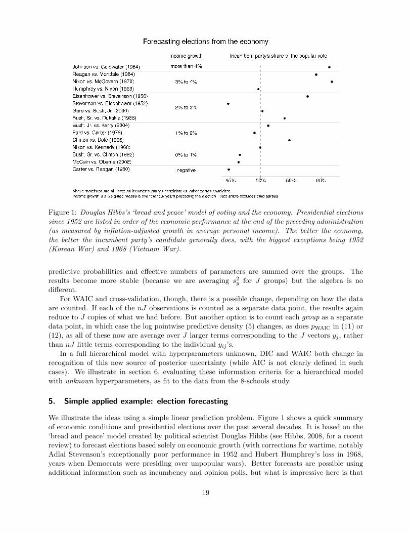
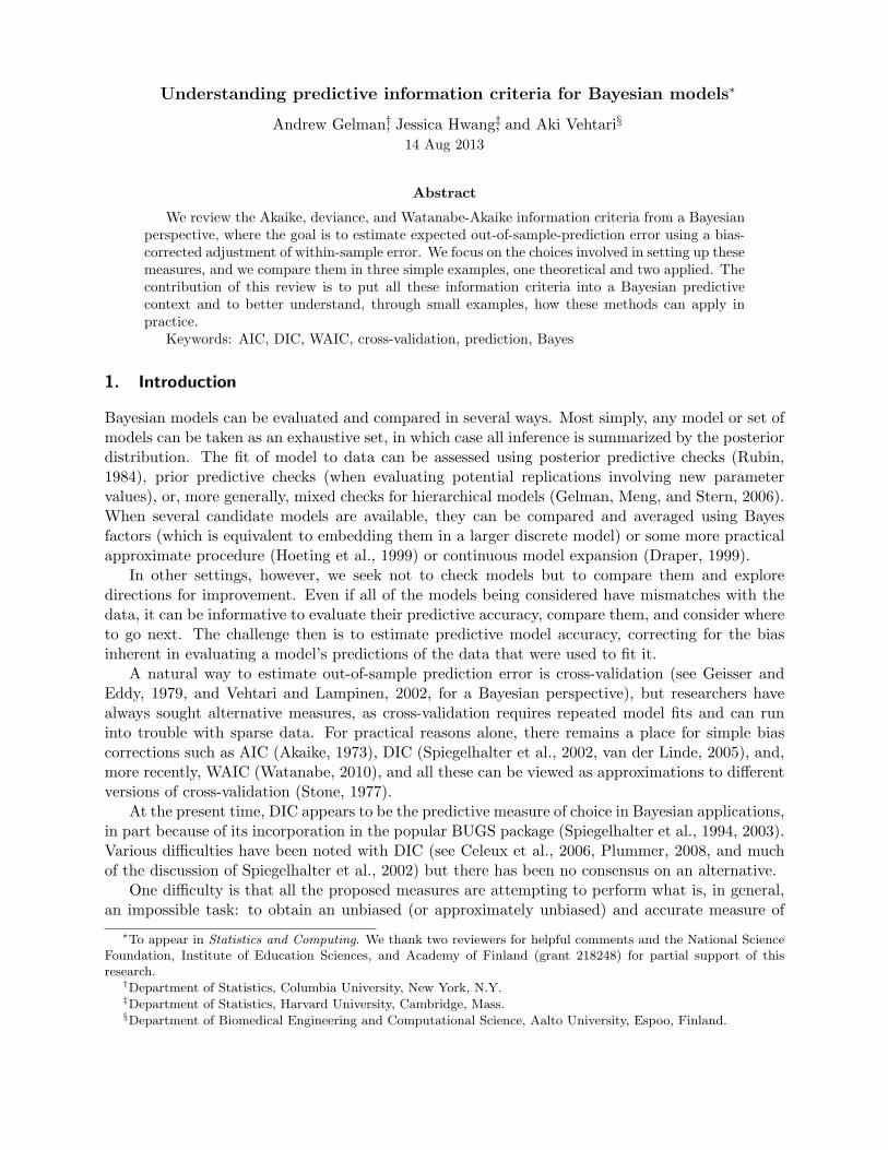
Figure 1: Douglas Hibbs’s ‘bread and peace’ model of voting and the economy. Presidential electionssince 1952 are listed in order of the economic performance at the end of the preceding administration(as measured by inflation-adjusted growth in average personal income). The better the economy,the better the incumbent party’s candidate generally does, with the biggest exceptions being 1952(Korean War) and 1968 (Vietnam War).
predictive probabilities and effective numbers of parameters are summed over the groups. Theresults become more stable (because we are averaging s2y for J groups) but the algebra is nodifferent.
For WAIC and cross-validation, though, there is a possible change, depending on how the dataare counted. If each of the nJ observations is counted as a separate data point, the results againreduce to J copies of what we had before. But another option is to count each group as a separatedata point, in which case the log pointwise predictive density (5) changes, as does pWAIC in (11) or(12), as all of these now are average over J larger terms corresponding to the J vectors yj , ratherthan nJ little terms corresponding to the individual yij ’s.
In a full hierarchical model with hyperparameters unknown, DIC and WAIC both change inrecognition of this new source of posterior uncertainty (while AIC is not clearly defined in suchcases). We illustrate in section 6, evaluating these information criteria for a hierarchical modelwith unknown hyperparameters, as fit to the data from the 8-schools study.
5. Simple applied example: election forecasting
We illustrate the ideas using a simple linear prediction problem. Figure 1 shows a quick summaryof economic conditions and presidential elections over the past several decades. It is based on the‘bread and peace’ model created by political scientist Douglas Hibbs (see Hibbs, 2008, for a recentreview) to forecast elections based solely on economic growth (with corrections for wartime, notablyAdlai Stevenson’s exceptionally poor performance in 1952 and Hubert Humphrey’s loss in 1968,years when Democrats were presiding over unpopular wars). Better forecasts are possible usingadditional information such as incumbency and opinion polls, but what is impressive here is that
19
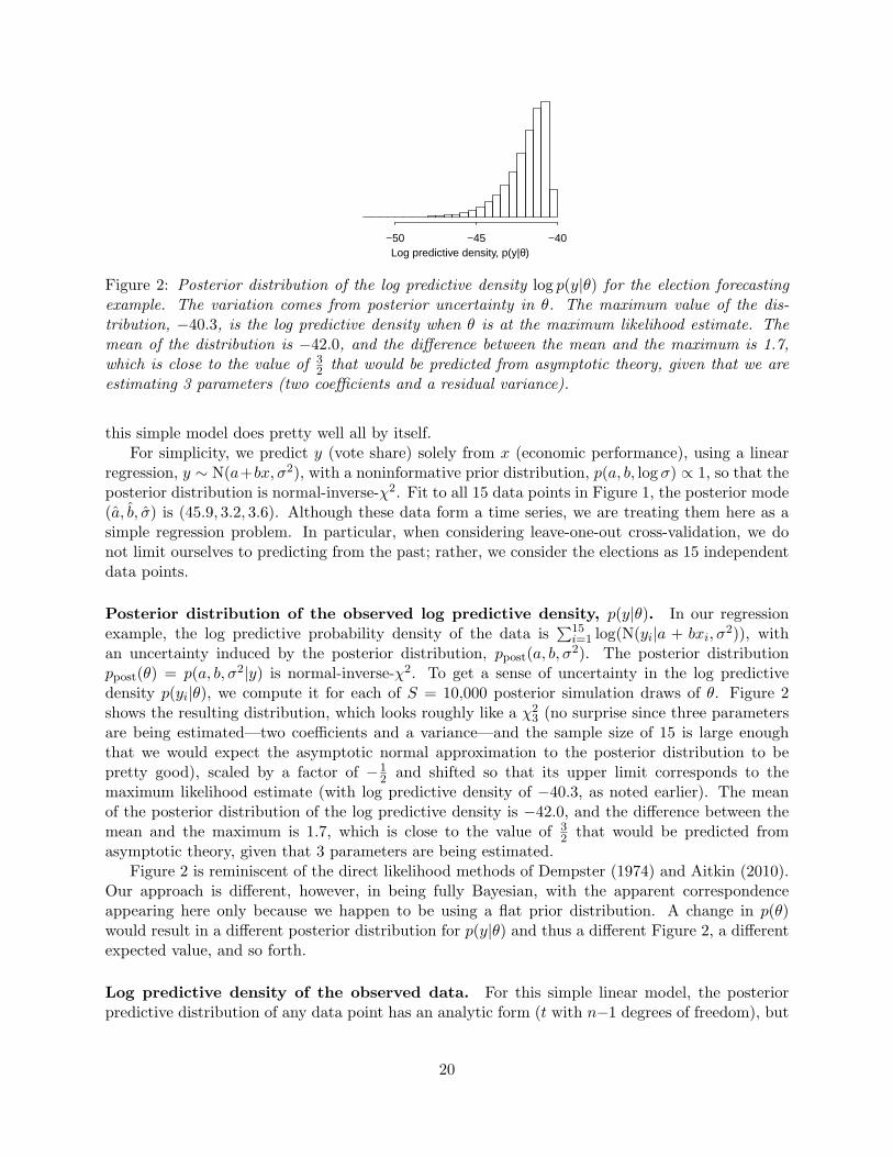
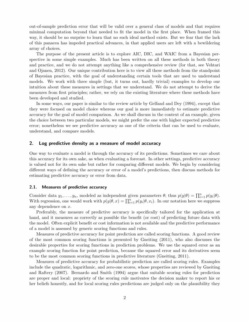
Log predictive density, p(y|θ)−50 −45 −40
Figure 2: Posterior distribution of the log predictive density log p(y|θ) for the election forecastingexample. The variation comes from posterior uncertainty in θ. The maximum value of the dis-tribution, −40.3, is the log predictive density when θ is at the maximum likelihood estimate. Themean of the distribution is −42.0, and the difference between the mean and the maximum is 1.7,which is close to the value of 3
2 that would be predicted from asymptotic theory, given that we areestimating 3 parameters (two coefficients and a residual variance).
this simple model does pretty well all by itself.For simplicity, we predict y (vote share) solely from x (economic performance), using a linear
regression, y ∼ N(a+bx, σ2), with a noninformative prior distribution, p(a, b, log σ) ∝ 1, so that theposterior distribution is normal-inverse-χ2. Fit to all 15 data points in Figure 1, the posterior mode(a, b, σ) is (45.9, 3.2, 3.6). Although these data form a time series, we are treating them here as asimple regression problem. In particular, when considering leave-one-out cross-validation, we donot limit ourselves to predicting from the past; rather, we consider the elections as 15 independentdata points.
Posterior distribution of the observed log predictive density, p(y|θ). In our regressionexample, the log predictive probability density of the data is
∑15i=1 log(N(yi|a + bxi, σ
2)), withan uncertainty induced by the posterior distribution, ppost(a, b, σ
2). The posterior distributionppost(θ) = p(a, b, σ2|y) is normal-inverse-χ2. To get a sense of uncertainty in the log predictivedensity p(yi|θ), we compute it for each of S = 10,000 posterior simulation draws of θ. Figure 2shows the resulting distribution, which looks roughly like a χ2
3 (no surprise since three parametersare being estimated—two coefficients and a variance—and the sample size of 15 is large enoughthat we would expect the asymptotic normal approximation to the posterior distribution to bepretty good), scaled by a factor of −1
2 and shifted so that its upper limit corresponds to themaximum likelihood estimate (with log predictive density of −40.3, as noted earlier). The meanof the posterior distribution of the log predictive density is −42.0, and the difference between themean and the maximum is 1.7, which is close to the value of 3
2 that would be predicted fromasymptotic theory, given that 3 parameters are being estimated.
Figure 2 is reminiscent of the direct likelihood methods of Dempster (1974) and Aitkin (2010).Our approach is different, however, in being fully Bayesian, with the apparent correspondenceappearing here only because we happen to be using a flat prior distribution. A change in p(θ)would result in a different posterior distribution for p(y|θ) and thus a different Figure 2, a differentexpected value, and so forth.
Log predictive density of the observed data. For this simple linear model, the posteriorpredictive distribution of any data point has an analytic form (t with n−1 degrees of freedom), but
20
it is easy enough to use the more general simulation-based computational formula (5). Calculatedeither way, the log pointwise predictive density is lppd = −40.9. Unsurprisingly, this number isslightly lower than the predictive density evaluated at the maximum likelihood estimate: averagingover uncertainty in the parameters yields a slightly lower probability for the observed data.
AIC. Fit to all 15 data points, the MLE (a, b, σ) is (45.9, 3.2, 3.6). Since 3 parameters are esti-mated, the value of elpdAIC is
15∑
i=1
log N(yi|45.9 + 3.2xi, 3.62) − 3 = − 43.3,
and AIC = −2 elpdAIC = 86.6.
DIC. The relevant formula is pDIC = 2 (log p(y|Epost(θ))− Epost(log p(y|θ))).The second of these terms is invariant to reparameterization; we calculate it as
Epost(y|θ) =1
S
S∑
s=1
15∑
i=1
log N(yi|as + bsxi, (σ
s)2) = −42.0,
based on a large number S of simulation draws.The first term is not invariant. With respect to the prior p(a, b, log σ) ∝ 1, the posterior means
of a and b are 45.9 and 3.2, the same as the maximum likelihood estimate. The posterior means ofσ, σ2, and log σ are E(σ|y) = 4.1, E(σ2|y) = 17.2, and E(log σ|y) = 1.4. Parameterizing using σ,we get
log p(y|Epost(θ)) =15∑
i=1
log N(yi|E(a|y) + E(b|y)xi, (E(σ|y))2) = −40.5,
which gives pDIC = 2(−40.5− (−42.0)) = 3.0, elpdDIC = log p(y|Epost(θ)) − pDIC = −40.5− 3.0 =
−43.5, and DIC = −2 elpdDIC = 87.0.
WAIC. The log pointwise predictive probability of the observed data under the fitted model is
lppd =15∑
i=1
log
(1
S
S∑
s=1
N(yi|as + bsxi, (σ
s)2)
)= −40.9.
The effective number of parameters can be calculated as
pWAIC1 = 2(lppd− Epost(y|θ)),= 2(−40.9− (−42.0)) = 2.2
or
pWAIC2 =15∑
i=1
V Ss=1 log N(yi|a
s + bsxi, (σs)2) = 2.7.
Then elppdWAIC1 = lppd − pWAIC1 = −40.9 − 2.2 = −43.1, and elppdWAIC2 = lppd − pWAIC2 =−40.9− 2.7 = −43.6, so WAIC is 86.2 or 87.2.
21
Estimated Standard errortreatment of effect
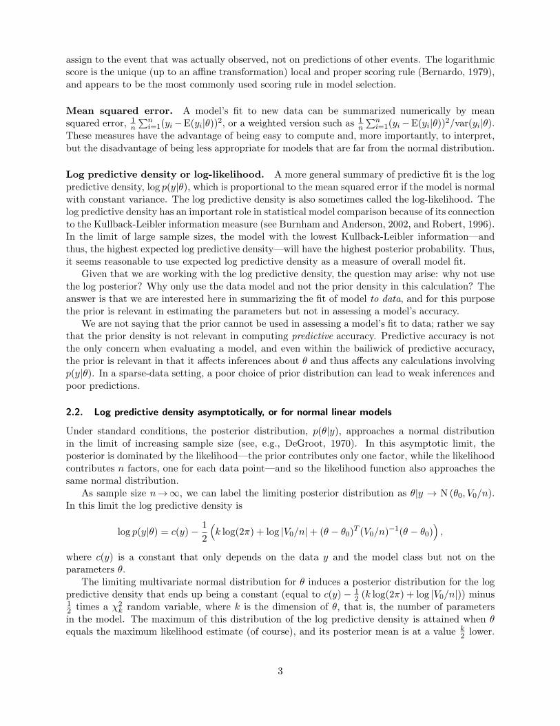
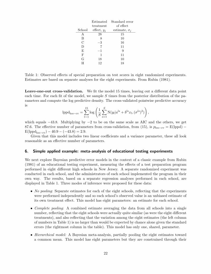
School effect, yj estimate, σj
A 28 15B 8 10C −3 16D 7 11E −1 9F 1 11G 18 10H 12 18
Table 1: Observed effects of special preparation on test scores in eight randomized experiments.Estimates are based on separate analyses for the eight experiments. From Rubin (1981).
Leave-one-out cross-validation. We fit the model 15 times, leaving out a different data pointeach time. For each fit of the model, we sample S times from the posterior distribution of the pa-rameters and compute the log predictive density. The cross-validated pointwise predictive accuracyis
lppdloo−cv =15∑
l=1
log
(1
S
S∑
s=1
N(yl|als + blsxl, (σ
ls)2)
),
which equals −43.8. Multiplying by −2 to be on the same scale as AIC and the others, we get87.6. The effective number of parameters from cross-validation, from (15), is ploo−cv = E(lppd) −E(lppdloo−cv)− 40.9− (−43.8) = 2.9.
Given that this model includes two linear coefficients and a variance parameter, these all lookreasonable as an effective number of parameters.
6. Simple applied example: meta-analysis of educational testing experiments
We next explore Bayesian predictive error models in the context of a classic example from Rubin(1981) of an educational testing experiment, measuring the effects of a test preparation programperformed in eight different high schools in New Jersey. A separate randomized experiment wasconducted in each school, and the administrators of each school implemented the program in theirown way. The results, based on a separate regression analyses performed in each school, aredisplayed in Table 1. Three modes of inference were proposed for these data:
• No pooling: Separate estimates for each of the eight schools, reflecting that the experimentswere performed independently and so each school’s observed value is an unbiased estimate ofits own treatment effect. This model has eight parameters: an estimate for each school.
• Complete pooling: A combined estimate averaging the data from all schools into a singlenumber, reflecting that the eight schools were actually quite similar (as were the eight differenttreatments), and also reflecting that the variation among the eight estimates (the left columnof numbers in Table 1) is no larger than would be expected by chance alone given the standarderrors (the rightmost column in the table). This model has only one, shared, parameter.
• Hierarchical model: A Bayesian meta-analysis, partially pooling the eight estimates towarda common mean. This model has eight parameters but they are constrained through their
22
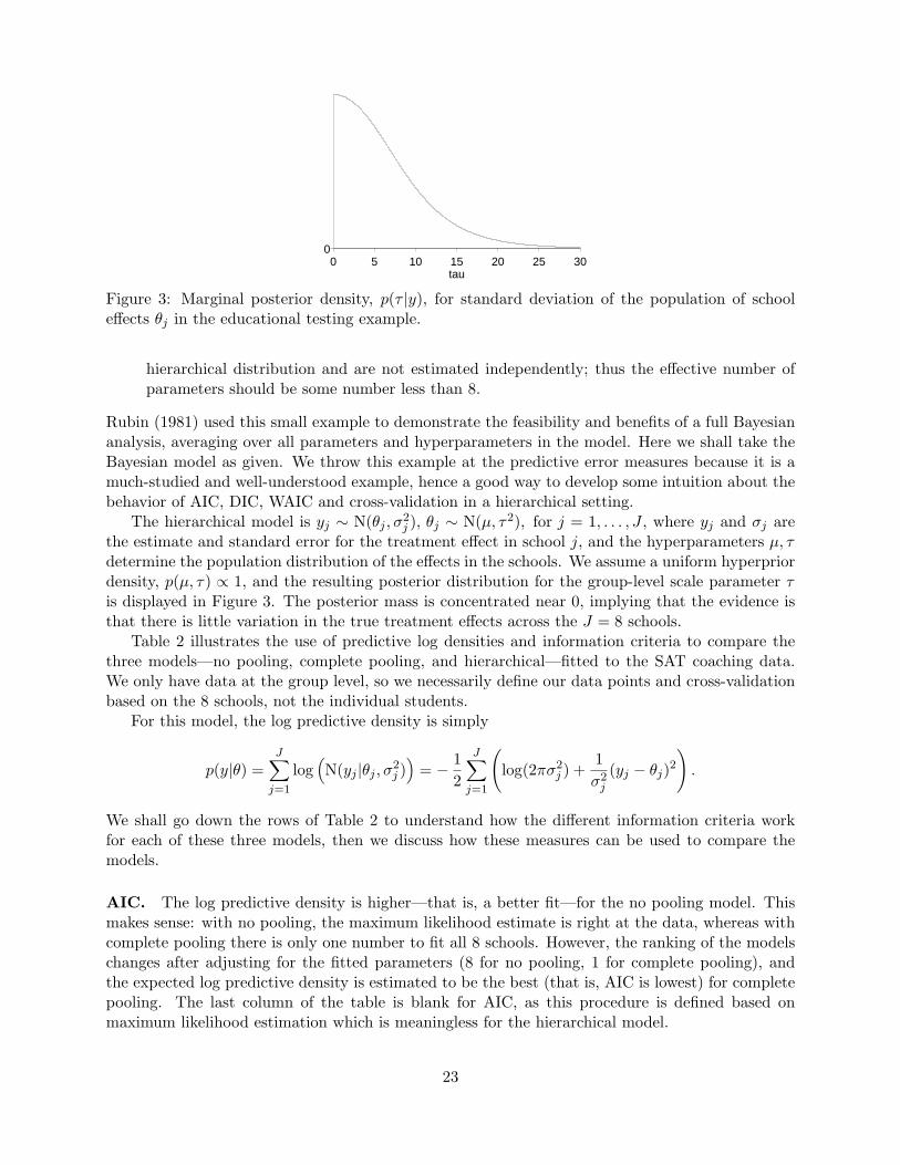
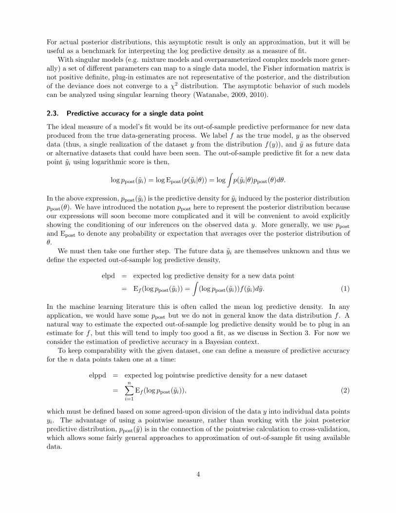
tau0 5 10 15 20 25 30
0
Figure 3: Marginal posterior density, p(τ |y), for standard deviation of the population of schooleffects θj in the educational testing example.
hierarchical distribution and are not estimated independently; thus the effective number ofparameters should be some number less than 8.
Rubin (1981) used this small example to demonstrate the feasibility and benefits of a full Bayesiananalysis, averaging over all parameters and hyperparameters in the model. Here we shall take theBayesian model as given. We throw this example at the predictive error measures because it is amuch-studied and well-understood example, hence a good way to develop some intuition about thebehavior of AIC, DIC, WAIC and cross-validation in a hierarchical setting.
The hierarchical model is yj ∼ N(θj , σ2j ), θj ∼ N(µ, τ2), for j = 1, . . . , J , where yj and σj are
the estimate and standard error for the treatment effect in school j, and the hyperparameters µ, τdetermine the population distribution of the effects in the schools. We assume a uniform hyperpriordensity, p(µ, τ) ∝ 1, and the resulting posterior distribution for the group-level scale parameter τis displayed in Figure 3. The posterior mass is concentrated near 0, implying that the evidence isthat there is little variation in the true treatment effects across the J = 8 schools.
Table 2 illustrates the use of predictive log densities and information criteria to compare thethree models—no pooling, complete pooling, and hierarchical—fitted to the SAT coaching data.We only have data at the group level, so we necessarily define our data points and cross-validationbased on the 8 schools, not the individual students.
For this model, the log predictive density is simply
p(y|θ) =J∑
j=1
log(N(yj |θj , σ
2j ))= −
1
2
J∑
j=1
(log(2πσ2
j ) +1
σ2j
(yj − θj)2
).
We shall go down the rows of Table 2 to understand how the different information criteria workfor each of these three models, then we discuss how these measures can be used to compare themodels.
AIC. The log predictive density is higher—that is, a better fit—for the no pooling model. Thismakes sense: with no pooling, the maximum likelihood estimate is right at the data, whereas withcomplete pooling there is only one number to fit all 8 schools. However, the ranking of the modelschanges after adjusting for the fitted parameters (8 for no pooling, 1 for complete pooling), andthe expected log predictive density is estimated to be the best (that is, AIC is lowest) for completepooling. The last column of the table is blank for AIC, as this procedure is defined based onmaximum likelihood estimation which is meaningless for the hierarchical model.
23
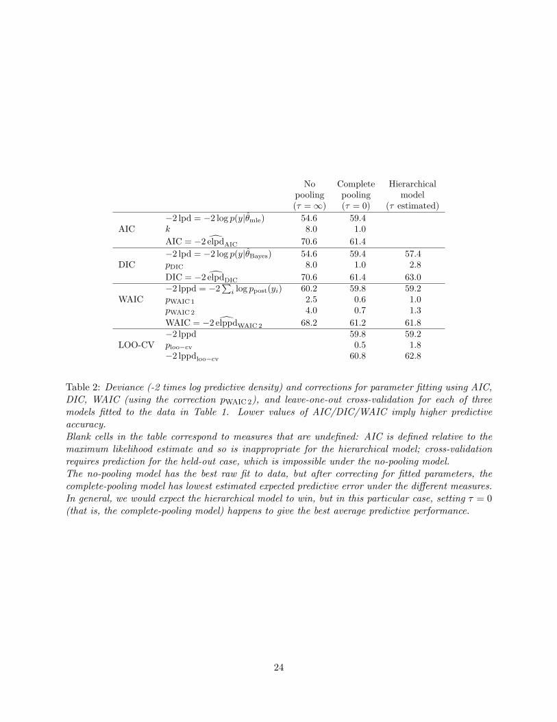
No Complete Hierarchicalpooling pooling model(τ = ∞) (τ = 0) (τ estimated)
−2 lpd = −2 log p(y|θmle) 54.6 59.4AIC k 8.0 1.0
AIC = −2 elpdAIC 70.6 61.4
−2 lpd = −2 log p(y|θBayes) 54.6 59.4 57.4DIC pDIC 8.0 1.0 2.8
DIC = −2 elpdDIC 70.6 61.4 63.0−2 lppd = −2
∑i log ppost(yi) 60.2 59.8 59.2
WAIC pWAIC1 2.5 0.6 1.0pWAIC2 4.0 0.7 1.3
WAIC = −2 elppdWAIC2 68.2 61.2 61.8−2 lppd 59.8 59.2
LOO-CV ploo−cv 0.5 1.8−2 lppdloo−cv 60.8 62.8
Table 2: Deviance (-2 times log predictive density) and corrections for parameter fitting using AIC,DIC, WAIC (using the correction pWAIC2), and leave-one-out cross-validation for each of threemodels fitted to the data in Table 1. Lower values of AIC/DIC/WAIC imply higher predictiveaccuracy.Blank cells in the table correspond to measures that are undefined: AIC is defined relative to themaximum likelihood estimate and so is inappropriate for the hierarchical model; cross-validationrequires prediction for the held-out case, which is impossible under the no-pooling model.The no-pooling model has the best raw fit to data, but after correcting for fitted parameters, thecomplete-pooling model has lowest estimated expected predictive error under the different measures.In general, we would expect the hierarchical model to win, but in this particular case, setting τ = 0(that is, the complete-pooling model) happens to give the best average predictive performance.
24
DIC. For the no-pooling and complete-pooling models with their flat priors, DIC gives resultsidentical to AIC (except for possible simulation variability, which we have essentially eliminatedhere by using a large number of posterior simulation draws). DIC for the hierarchical model givessomething in between: a direct fit to data (lpd) that is better than complete pooling but not asgood as the (overfit) no pooling, and an effective number of parameters of 2.8, closer to 1 than to8, which makes sense given that the estimated school effects are pooled almost all the way backto their common mean. Adding in the correction for fitting, complete pooling wins, which makessense given that in this case the data are consistent with zero between-group variance.
WAIC. This fully Bayesian measure gives results similar to DIC. The fit to observed data isslightly worse for each model (that is, the numbers for lppd are slightly more negative than thecorresponding values for lpd, higher up in the table), accounting for the fact that the posteriorpredictive density has a wider distribution and thus has lower density values at the mode, comparedto the predictive density conditional on the point estimate. However, the correction for effectivenumber of parameters is lower (for no pooling and the hierarchical model, pWAIC is about half ofpDIC), consistent with the theoretical behavior of WAIC when there is only a single data point perparameter, while for complete pooling, pWAIC is only a bit less than 1, roughly consistent with whatwe would expect from a sample size of 8. For all three models here, pWAIC is much less than pDIC,with this difference arising from the fact that the lppd in WAIC is already accounting for much ofthe uncertainty arising from parameter estimation.
Cross-validation. For this example it is impossible to cross-validate the no-pooling model as itwould require the impossible task of obtaining a prediction from a held-out school given the otherseven. This illustrates one main difference to information criteria, which assume new predictionfor these same schools and thus work also in no-pooling model. For complete pooling and for thehierarchical model, we can perform leave-one-out cross-validation directly. In this model the localprediction of cross-validation is based only on the information coming from the other schools, whilethe local prediction in WAIC is based on the local observation as well as the information comingfrom the other schools. In both cases the prediction is for unknown future data, but the amountof information used is different and thus predictive performance estimates differ more when thehierarchical prior becomes more vague (with the difference going to infinity as the hierarchical priorbecomes uninformative, to yield the no-pooling model). This example shows that it is importantto consider which prediction task we are interested in and that it is not clear what n means inasymptotic results that feature terms such as o(n−1).
Comparing the three models. For this particular dataset, complete pooling wins the expectedout-of-sample prediction competition. Typically it is best to estimate the hierarchical variance but,in this case, τ = 0 is the best fit to the data, and this is reflected in the center column in Table 2,where the expected log predictive densities are higher than for no pooling or complete pooling.
That said, we still prefer the hierarchical model here, because we do not believe that τ istruly zero. For example, the estimated effect in school A is 28 (with a standard error of 15) andthe estimate in school C is −3 (with a standard error of 16). This difference is not statisticallysignificant and, indeed, the data are consistent with there being zero variation of effects betweenschools; nonetheless we would feel uncomfortable, for example, stating that the posterior probabilityis 0.5 that the effect in school C is larger than the effect in school A, given that data that show schoolA looking better. It might, however, be preferable to use a more informative prior distribution onτ , given that very large values are both substantively implausible and also contribute to some of
25
the predictive uncertainty under this model.In general, predictive accuracy measures are useful in parallel with posterior predictive checks
to see if there are important patterns in the data that are not captured by each model. As withpredictive checking, the log score can be computed in different ways for a hierarchical model de-pending on whether the parameters θ and replications yrep correspond to estimates and replicationsof new data from the existing groups (as we have performed the calculations in the above example)or new groups (additional schools from the N(µ, τ2) distribution in the above example).
7. Discussion
There are generally many options in setting up a model for any applied problem. Our usualapproach is to start with a simple model that uses only some of the available information—forexample, not using some possible predictors in a regression, fitting a normal model to discretedata, or ignoring evidence of unequal variances and fitting a simple equal-variance model. Once wehave successfully fitted a simple model, we can check its fit to data and then alter or expand it asappropriate.
There are two typical scenarios in which models are compared. First, when a model is expanded,it is natural to compare the smaller to the larger model and assess what has been gained byexpanding the model (or, conversely, if a model is simplified, to assess what was lost). Thisgeneralizes into the problem of comparing a set of nested models and judging how much complexityis necessary to fit the data.
In comparing nested models, the larger model typically has the advantage of making more senseand fitting the data better but the disadvantage of being more difficult to understand and compute.The key questions of model comparison are typically: (1) is the improvement in fit large enoughto justify the additional difficulty in fitting, and (2) is the prior distribution on the additionalparameters reasonable?
The second scenario of model comparison is between two or more nonnested models—neithermodel generalizes the other. One might compare regressions that use different sets of predictors tofit the same data, for example, modeling political behavior using information based on past votingresults or on demographics. In these settings, we are typically not interested in choosing one of themodels—it would be better, both in substantive and predictive terms, to construct a larger modelthat includes both as special cases, including both sets of predictors and also potential interactionsin a larger regression, possibly with an informative prior distribution if needed to control theestimation of all the extra parameters. However, it can be useful to compare the fit of the differentmodels, to see how either set of predictors performs when considered alone.
In any case, when evaluating models in this way, it is important to adjust for overfitting,especially when comparing models that vary greatly in their complexity, hence the value of themethods discussed in this article.
7.1. Evaluating predictive error comparisons
When comparing models in their predictive accuracy, two issues arise, which might be called sta-tistical and practical significance. Lack of statistical significance arises from uncertainty in theestimates of comparative out-of-sample prediction accuracy and is ultimately associated with vari-ation in individual prediction errors which manifests itself in averages for any finite dataset. Someasymptotic theory suggests that the sampling variance of any estimate of average prediction errorwill be of order 1, so that, roughly speaking, differences of less than 1 could typically be attributedto chance, but according to Ripley (1996), this asymptotic result does not necessarily hold for
26

nonnested models. A practical estimate of related sampling uncertainty can be obtained by analyz-ing the variation in the expected log predictive densities elppdi using parametric or nonparametricapproaches (Vehtari and Lampinen, 2002).
Practical significance depends on the purposes to which a model will be used. Sometimes itmay be possible to use an application-specific scoring function that is so familiar for subject-matterexperts that they can interpret the practical significance of differences. For example, epidemiologistsare used to looking at differences in area under receiver operating characteristic curve (AUC) forclassification and survival models. In settings without such conventional measures, it is not alwaysclear how to interpret the magnitude of a difference in log predictive probability when comparingtwo models. Is a difference of 2 important? 10? 100? One way to understand such differences isto calibrate based on simpler models (McCulloch, 1989). For example, consider two models for asurvey of n voters in an American election, with one model being completely empty (predictingp = 0.5 for each voter to support either party) and the other correctly assigning probabilities of0.4 and 0.6 (one way or another) to the voters. Setting aside uncertainties involved in fitting,the expected log predictive probability is log(0.5) = −0.693 per respondent for the first model and0.6 log(0.6)+0.4 log(0.4) = −0.673 per respondent for the second model. The expected improvementin log predictive probability from fitting the better model is then 0.02n. So, for n = 1000, thiscomes to an improvement of 20, but for n = 10 the predictive improvement is only 2. This wouldseem to accord with intuition: going from 50/50 to 60/40 is a clear win in a large sample, but in asmaller predictive dataset the modeling benefit would be hard to see amid the noise.
In our studies of public opinion and epidemiology, we have seen cases where a model that islarger and better (in the sense of giving more reasonable predictions) does not appear dominant inthe predictive comparisons. This can happen because the improvements are small on an absolutescale (for example, changing the predicted average response among a particular category of thepopulation from 55% Yes to 60% Yes) and concentrated in only a few subsets of the population(those for which there is enough data so that a more complicated model yields noticeably differentpredictions). Average out-of-sample prediction error can be a useful measure but it does not tellthe whole story of model fit.
7.2. Selection-induced bias
Cross-validation and information criteria make a correction for using the data twice (in constructingthe posterior and in model assessment) and obtain asymptotically unbiased estimates of predictiveperformance for a given model. However, when these methods are used for model selection, thepredictive performance estimate of the selected model is biased due to the selection process (seereferences in Vehtari and Ojanen, 2012).
If the number of compared models is small, the bias is small, but if the number of candidatemodels is very large (for example, the number of models grows exponentially as the number ofobservations n grows, or the number of covariates p ≫ ln(n) in covariate selection) a model selectionprocedure can strongly overfit the data. It is possible to estimate the selection-induced bias andobtain unbiased estimates, for example by using another level of cross-validation. This does not,however, prevent the model selection procedure from possibly overfitting to the observations andconsequently selecting models with suboptimal predictive performance. This is one reason we viewcross-validation and information criteria as an approach for understanding fitted models ratherthan for choosing among them.
27
7.3. Challenges and conclusions
The current state of the art of measurement of predictive model fit remains unsatisfying. Formu-las such as AIC, DIC, and WAIC fail in various examples: AIC does not work in settings withstrong prior information, DIC gives nonsensical results when the posterior distribution is not wellsummarized by its mean, and WAIC relies on a data partition that would cause difficulties withstructured models such as for spatial or network data. Cross-validation is appealing but can becomputationally expensive and also is not always well defined in dependent data settings.
For these reasons, Bayesian statisticians do not always use predictive error comparisons in ap-plied work, but we recognize that there are times when it can be useful to compare highly dissimilarmodels, and, for that purpose, predictive comparisons can make sense. In addition, measures ofeffective numbers of parameters are appealing tools for understanding statistical procedures, es-pecially when considering models such as splines and Gaussian processes that have complicateddependence structures and thus no obvious formulas to summarize model complexity.
Thus we see the value of the methods described here, for all their flaws. Right now our preferredchoice is cross-validation, with WAIC as a fast and computationally-convenient alternative. WAICis fully Bayesian (using the posterior distribution rather than a point estimate), gives reasonableresults in the examples we have considered here, and has a more-or-less explicit connection to cross-validation, as can be seen its formulation based on pointwise predictive density (Watanabe, 2010,Vehtari and Ojanen, 2012). A useful goal of future research would be a bridge between WAIC andcross-validation with much of the speed of the former and robustness of the latter.
References
Aitkin, M. (2010). Statistical Inference: An Integrated Bayesian/Likelihood Approach. London:Chapman & Hall.
Akaike, H. (1973). Information theory and an extension of the maximum likelihood principle. InProceedings of the Second International Symposium on Information Theory, ed. B. N. Petrovand F. Csaki, 267–281. Budapest: Akademiai Kiado. Reprinted in Breakthroughs in Statistics,ed. S. Kotz, 610–624. New York: Springer (1992).
Ando, T., and Tsay, R. (2010). Predictive likelihood for Bayesian model selection and averaging.International Journal of Forecasting 26, 744–763.
Bernardo, J. M. (1979). Expected information as expected utility. Annals of Statistics 7, 686–690.
Bernardo, J. M., and Smith, A. F. M. (1994). Bayesian Theory. New York: Wiley.
Burman, P. (1989). A comparative study of ordinary cross-validation, v-fold cross-validation andthe repeated learning-testing methods. Biometrika 76, 503–514.
Burman, P., Chow, E., and Nolan, D. (1994). A cross-validatory method for dependent data.Biometrika 81, 351–358.
Burnham, K. P., and Anderson, D. R. (2002). Model Selection and Multimodel Inference: APractical Information Theoretic Approach. New York: Springer.
Celeux, G., Forbes, F., Robert, C. and Titterington, D. (2006). Deviance information criteria formissing data models. Bayesian Analysis 1, 651-706.
DeGroot, M. H. (1970). Optimal Statistical Decisions. New York: McGraw-Hill.
Dempster, A .P. (1974). The direct use of likelihood for significance testing. Proceedings of Confer-ence on Foundational Questions in Statistical Inference, Department of Theoretical Statistics:University of Aarhus, 335–352.
28
Draper, D. (1999). Model uncertainty yes, discrete model averaging maybe. Statistical Science 14,405–409.
Efron, B., and Tibshirani, R. (1993). An Introduction to the Bootstrap. New York: Chapman &Hall.
Geisser, S., and Eddy, W. (1979). A predictive approach to model selection. Journal of theAmerican Statistical Association 74, 153–160.
Gelfand, A., and Dey, D. (1994). Bayesian model choice: asymptotics and exact calculations.Journal of the Royal Statistical Society B 56, 501–514.
Gelman, A., Carlin, J. B., Stern, H. S., and Rubin, D. B. (2003). Bayesian Data Analysis, secondedition. London: CRC Press.
Gelman, A., Meng, X. L., and Stern, H. S. (1996). Posterior predictive assessment of model fitnessvia realized discrepancies (with discussion). Statistica Sinica 6, 733–807.
Gelman, A., and Shalizi, C. (2013). Philosophy and the practice of Bayesian statistics (withdiscussion). British Journal of Mathematical and Statistical Psychology 66, 8–80.
Gneiting, T. (2011). Making and evaluating point forecasts. Journal of the American StatisticalAssociation 106, 746–762.
Gneiting, T., and Raftery, A. E. (2007). Strictly proper scoring rules, prediction, and estimation.Journal of American Statistical Association 102, 359–378.
Hibbs, D. (2008). Implications of the ‘bread and peace’ model for the 2008 U.S. presidential election.Public Choice 137, 1–10.
Hoeting, J., Madigan, D., Raftery, A. E., and Volinsky, C. (1999). Bayesian model averaging (withdiscussion). Statistical Science 14, 382–417.
Jones, H. E. and Spiegelhalter, D. J. (2012). Improved probabilistic prediction of healthcare perfor-mance indicators using bidirectional smoothing models. Journal of the Royal Statistical SocietyA 175, 729–747.
McCulloch, R. E. (1989). Local model influence. Journal of the American Statistical Association84, 473-478.
Plummer, M. (2008). Penalized loss functions for Bayesian model comparison. Biostatistics 9,523–539.
Ripley, B. D. (1996). Statistical Pattern Recognition and Neural Networks. Cambridge UniversityPress.
Robert, C. P. (1996). Intrinsic losses. Theory and Decision 40, 191–214.
Rubin, D. B. (1981). Estimation in parallel randomized experiments. Journal of EducationalStatistics 6, 377–401.
Rubin, D. B. (1984). Bayesianly justifiable and relevant frequency calculations for the appliedstatistician. Annals of Statistics 12, 1151–1172.
Schwarz, G. E. (1978). Estimating the dimension of a model. Annals of Statistics 6, 461–464.
Shibata, R. (1989). Statistical aspects of model selection. In From Data to Model, ed. J. C. Willems,215–240. Springer-Verlag.
Spiegelhalter, D. J., Best, N. G., Carlin, B. P., and van der Linde, A. (2002). Bayesian measuresof model complexity and fit (with discussion). Journal of the Royal Statistical Society B.
Spiegelhalter, D., Thomas, A., Best, N., Gilks, W., and Lunn, D. (1994, 2003). BUGS: Bayesianinference using Gibbs sampling. MRC Biostatistics Unit, Cambridge, England.http://www.mrc-bsu.cam.ac.uk/bugs/
29

Stone, M. (1977). An asymptotic equivalence of choice of model cross-validation and Akaike’scriterion. Journal of the Royal Statistical Society B 36, 44–47.
van der Linde, A. (2005). DIC in variable selection. Statistica Neerlandica 1, 45–56.
Vehtari, A., and Lampinen, J. (2002). Bayesian model assessment and comparison using cross-validation predictive densities. Neural Computation 14, 2439–2468.
Vehtari, A., and Ojanen, J. (2012). A survey of Bayesian predictive methods for model assessment,selection and comparison. Statistics Surveys 6, 142–228.
Watanabe, S. (2009). Algebraic Geometry and Statistical Learning Theory. Cambridge UniversityPress.
Watanabe, S. (2010). Asymptotic equivalence of Bayes cross validation and widely applicableinformation criterion in singular learning theory. Journal of Machine Learning Research 11,3571–3594.
Watanabe, S. (2013). A widely applicable Bayesian information criterion. Journal of MachineLearning Research 14, 867–897.
30