understanding monetary policy implementation/media/richmondfedorg/...circulation. forecasting errors...
TRANSCRIPT

Economic Quarterly—Volume 94, Number 3—Summer 2008—Pages 235–263
Understanding MonetaryPolicy Implementation
Huberto M. Ennis and Todd Keister
O ver the last two decades, central banks around the world have adopteda common approach to monetary policy that involves targeting thevalue of a short-term interest rate. In the United States, for example,
the Federal Open Market Committee (FOMC) announces a rate that it wishesto prevail in the federal funds market, where commercial banks lend balancesheld at the Federal Reserve to each other overnight. Changes in this short-term interest rate eventually translate into changes in other interest rates in theeconomy and thereby influence the overall level of prices and of real economicactivity.
Once a target interest rate is announced, the problem of implementationarises: How can a central bank ensure that the relevant market interest ratestays at or near the chosen target? The Federal Reserve has a variety of toolsavailable to influence the behavior of the interest rate in the federal fundsmarket (called the fed funds rate). In general, the Fed aims to adjust the totalsupply of reserve balances so that it equals demand at exactly the target rateof interest. This process necessarily involves some estimation, since the Feddoes not know the exact demand for reserve balances, nor does it completelycontrol the supply in the market.
A critical issue in the implementation process, therefore, is the sensitivityof the market interest rate to unanticipated changes in supply and/or demand.
Some of the material in this article resulted from our participation in the Federal ReserveSystem task force created to study paying interest on reserves. We are very grateful to theother members of this group, who patiently taught us many of the things that we discuss here.We also would like to thank Kevin Bryan, Yash Mehra, Rafael Repullo, John Walter, JohnWeinberg, and the participants at the 2008 Columbia Business School/New York Fed confer-ence on “The Role of Money Markets” for useful comments on a previous draft. All remain-ing errors are, of course, our own. The views expressed here do not necessarily representthose of the Federal Reserve Bank of New York, the Federal Reserve Bank of Richmond,or the Federal Reserve System. Ennis is on leave from the Richmond Fed at UniversityCarlos III of Madrid and Keister is at the Federal Reserve Bank of New York. E-mails:[email protected], [email protected].

236 Federal Reserve Bank of Richmond Economic Quarterly
If small estimation errors lead to large swings in the interest rate, a centralbank will find it difficult to effectively implement monetary policy, that is, toconsistently hit the target rate. The degree of sensitivity depends on a varietyof factors related to the design of the implementation process, such as the timeperiod over which banks are required to hold reserves and the interest rate, ifany, that a central bank pays on reserve balances.
The ability to hit a target interest rate consistently plays a critical role in acentral bank’s communication policy. The overall effectiveness of monetarypolicy depends, in part, on individuals’ perceptions of the central bank’s ac-tions and objectives. If the market interest rate were to deviate consistentlyfrom the central bank’s announced target, individuals might question whetherthese deviations simply represent glitches in the implementation process orwhether they instead represent an unannounced change in the stance of mon-etary policy. Sustained deviations of the average fed funds rate from theFOMC’s target in August 2007, for example, led some media commentatorsto claim that the Fed had engaged in a “stealth easing,” taking actions thatlowered the market interest rate without announcing a change in the officialtarget.1 In such times, the ability to hit a target interest rate consistently allowsthe central bank to clearly (and credibly) communicate its policy to marketparticipants.
Under most circumstances, the Fed changes the total supply of reservebalances available to commercial banks by exchanging government bondsor other securities for reserves in an open market operation. Occasionally,the Fed also provides reserves directly to certain banks through its discountwindow. In some situations, the Fed has developed other, ad hoc methodsof influencing the supply and distribution of reserves in the market. Forexample, during the recent period of financial turmoil, the market’s ability tosmoothly distribute reserves across banks became partially impaired, whichled to significant fluctuations in the average fed funds rate both during the dayand across days. In December 2007, partly to address these problems, the Fedintroduced the Term Auction Facility (TAF), a bimonthly auction of a fixedquantity of reserve balances to all banks eligible to borrow at the discountwindow. In principle, the TAF has increased these banks’ ability to accessreserves directly and, in this way, has helped ease the pressure on the marketto redistribute reserves and avoid abnormal fluctuations in the market rate.Such operations, of course, need to be managed so as to achieve the ultimategoal of implementing the chosen target interest rate. Balancing the demandand supply of reserves is at the very core of this problem.
This article presents a simple analytical framework for understanding theprocess of monetary policy implementation and the factors that influence a
1 See, for example, “A ‘Stealth Easing’ by the Fed?” (Coy 2007).
H. M. Ennis and T. Keister: Monetary Policy Implementation 237
central bank’s ability to keep the market interest rate close to a target level.We present this framework graphically, focusing on how various features ofthe implementation process affect the sensitivity of the market interest rate tounanticipated changes in supply or demand. We discuss the current approachused by the Fed, including the use of reserve maintenance periods to decreasethis sensitivity. We also show how this framework can be used to study a widerange of issues related to monetary policy implementation.
In 2006, the U.S. Congress enacted legislation that will give the Fed theauthority to pay interest on reserve balances beginning in October 2011.2
We use our simple framework to illustrate how the ability to pay interest onreserves can be a useful policy tool for a central bank. In particular, we showhow paying interest on reserves can decrease the sensitivity of the marketinterest rate to estimation errors and, thus, enable a central bank to betterachieve its desired interest rate.
The model we present uses the basic approach to reserve managementintroduced by Poole (1968) and subsequently advanced by many others (see,for example, Dotsey 1991; Guthrie and Wright 2000; Bartolini, Bertola, andPrati 2002; and Clouse and Dow 2002). The specific details of our formaliza-tion closely follow those in Ennis and Weinberg (2007), after some additionalsimplifications that allow us to conduct all of our analysis graphically. Ennisand Weinberg (2007) focused on the interplay between daylight credit andthe Fed’s overnight treatment of bank reserves. In this article, we take a morecomprehensive view of the process of monetary policy implementation and weinvestigate several important topics, such as the role of reserve maintenanceperiods, which were left unexplored by Ennis and Weinberg (2007).
1. U.S. MONETARY POLICY IMPLEMENTATION
Banks hold reserve balances in accounts at the Federal Reserve in order tosatisfy reserve requirements and to be able to make interbank payments. Dur-ing the day, banks can also access funds by obtaining an overdraft from theirreserve accounts at the Fed. The terms by which the Fed provides daylightcredit are one of the factors determining the demand for reserves by banks.
To adjust their reserve holdings, banks can borrow and lend balances inthe fed funds market, which operates weekdays from 9:30 a.m. to 6:30 p.m.A bank wanting to decrease its reserve holdings, for example, can do so in thismarket by making unsecured, overnight loans to other banks.
The fed funds market plays a crucial role in monetary policy implementa-tion because this is where the Federal Reserve intervenes to pursue its policyobjectives. The stance of monetary policy is decided by the FOMC, which
2 After this article was written, the effective date for the authority to pay interest on reserveswas moved to October 1, 2008, by the Emergency Economic Stabilization Act of 2008.

238 Federal Reserve Bank of Richmond Economic Quarterly
selects a target for the overnight interest rate prevailing in this market. TheCommittee then instructs the Open Market Desk to adjust, via open marketoperations, the supply of reserve balances so as to steer the market interestrate toward the selected target.3
The Desk conducts open market operations largely by arranging repur-chase agreements (repos) with primary securities dealers in a sealed-bid,discriminatory price auction. Repos involve using reserve balances to pur-chase securities with the explicit agreement that the transaction will bereversed at maturity. Repos usually have overnight maturity, but the Deskalso employs other maturities (for example, two-day and two-week repos arecommonly used). Open market operations are typically conducted early inthe morning when the market for repos is most active.
The new reserves created in an open market operation are deposited in theparticipating securities dealers’ bank accounts and, hence, increase the totalsupply of reserves in the banking system. In this way, each day the Desktries to move the supply of reserve balances as close as possible to the levelthat would leave the market-clearing interest rate equal to the target rate. Anessential step in this process is accurately forecasting both aggregate reservedemand and those changes in the existing supply of reserve balances that aredue to autonomous factors beyond the Fed’s control, such as payments intoand out of the Treasury’s account and changes in the quantity of currency incirculation. Forecasting errors will lead the actual supply of reserve balancesto deviate from the intended level and, hence, will cause the market rate todiverge from the target rate, even if reserve demand is perfectly anticipated.
Reserve requirements in the United States are calculated as a proportionof the quantity of transaction deposits on a bank’s balance sheet during a two-week computation period prior to the start of the maintenance period. Theserequirements can be met through a combination of vault cash and reservebalances held at the Fed. During the two-week reserve maintenance period,a bank’s end-of-day reserve balances must, on average, equal the reserverequirement minus the quantity of vault cash held during the computationperiod. Reserve requirements make a large portion of the demand for reservebalances fairly predictable, which simplifies monetary policy implementation.
Reserve maintenance periods allow banks to spread out their reserve hold-ings over time without having to scramble for funds to meet a requirement atthe end of each day. However, near the end of the maintenance period, thisaveraging effect tends to lose force. On the last day of the period, a bank hassome level of remaining requirement that must be met on that day. This gen-erates a fairly inelastic demand for reserve balances and makes implementinga target interest rate more challenging. For this reason, the Fed allows banks
3 See Hilton and Hrung (2007) for a more detailed overview of the Fed’s monetary policyimplementation procedures.
H. M. Ennis and T. Keister: Monetary Policy Implementation 239
holding excess or deficient balances at the end of a maintenance period to carryover those balances and use them to satisfy up to 4 percent of their requirementin the following period.
If a bank finds itself short of reserves at the end of the maintenance period,even after taking into account the carryover possibilities, it has several options.It can try to find a counterparty late in the day offering an acceptable interestrate. However, this may not be feasible because of an aggregate shortage ofreserve balances or because of the existence of trading frictions in this market.A second alternative is to borrow at the discount window of its correspondingFederal Reserve Bank.4 The discount window offers collateralized overnightloans of reserves to banks that have previously pledged appropriate collateral.Discount window loans are typically charged an interest rate that is 100 basispoints above the target fed funds rate, although changing the size of this gapis possible and has been used, at times, as a policy instrument. Finally, ifthe bank does not have the appropriate collateral or chooses not to borrowat the discount window for other reasons, it will be charged a penalty feeproportional to the amount of the shortage.
Currently, banks earn no interest on the reserve balances they hold intheir accounts at the Federal Reserve.5 This situation may soon change: TheFinancial Services Regulatory Relief Act of 2006 allows the Fed to beginpaying interest on reserve balances in October 2011. The Act also includesprovisions that give the Fed more flexibility in determining reserve require-ments, including the ability to eliminate the requirements altogether. Thus,this legislation opens the door to potentially substantial changes in the waythe Fed implements monetary policy. To evaluate the best approach within thenew, broader set of alternatives, it seems useful to develop a simple analyticalframework that is able to address many of the relevant aspects of the problem.We introduce and discuss such a framework in the sections that follow.
2. THE DEMAND FOR RESERVES
In this section, we present a simple framework that is useful for understandingbanks’demand for reserves. In this framework, a bank holds reserves primarilyto satisfy reserve requirements, although other factors, such as the desire tomake interbank payments, may also play a role. Since banks cannot fullypredict the timing of payments, they face uncertainty about the net outflowsfrom their reserve accounts and, therefore, are typically unable to exactlysatisfy their reserve requirements. Instead, they must balance the possibility
4 There are 12 regions and corresponding Reserve Banks in the Federal Reserve System. Foreach commercial bank, the corresponding Reserve Bank is determined by the region where thecommercial bank is headquartered.
5 See footnote 2.

240 Federal Reserve Bank of Richmond Economic Quarterly
of holding excess reserve balances—and the associated opportunity cost—against the possibility of being penalized for a reserve deficiency. A bank’sdemand for reserves results from optimally balancing these two concerns.
The Basic Framework
We assume banks are risk-neutral and maximize expected profits. At thebeginning of the day, banks can borrow and lend reserves in a competitiveinterbank market. Let R be the quantity of reserves chosen by a bank inthe interbank market. The central bank affects the supply of reserves in thismarket by conducting open market operations. Total reserve supply is equalto the quantity set by the central bank through its operations, adjusted by apotentially random amount to reflect unpredictable changes in autonomousfactors.
During the day, each bank makes payments to and receives payments fromother banks. To keep things as simple as possible, suppose that each bankwill make exactly one payment and receive exactly one payment during the“middle” part of the day. Furthermore, suppose that these two payment flowsare of exactly the same size, PD > 0, and that this size is nonstochastic. How-ever, the order in which these payments occur during the day is random; somebanks will receive the incoming payment before making the outgoing one,while others will make the outgoing payment before receiving the incomingone.
At the end of the day, after the interbank market has closed, each bankexperiences another payment shock, P , that affects its end-of-day reservebalance. The value of P can be either positive, indicating a net outflow offunds, or negative, indicating a net inflow of funds. We assume that thepayment shock, P , is uniformly distributed on the interval
[−P , P]. The
value of this shock is not yet known when the interbank market is open; hence,a bank’s demand for reserves in this market is affected by the distribution ofthe payment shock and not the realization.
We assume, as a starting point, that a bank must meet a given reserverequirement, K , at the end of each day.6 If the bank finds itself holding fewerthan K reserves at the end of the day, after the payment shock P has beenrealized, it must borrow funds at a “penalty” rate of interest, rP , to satisfy therequirement. This rate can be thought of as the rate charged by the centralbank on discount window loans, adjusted to take into account any “stigma”associated with using this facility. In reality, a bank may pay a deficiencyfee instead of borrowing from the discount window or it may borrow funds
6 We discuss more complicated systems of reserve requirements later, including multiple-daymaintenance periods. For the logic in the derivations that follow, the particular value of K doesnot matter. The case of K = 0 corresponds to a system without reserve requirements.
H. M. Ennis and T. Keister: Monetary Policy Implementation 241
in the interbank market very late in the day when this market is illiquid. Inthe model, the rate rP simply represents the cost associated with a late-dayreserve deficiency, whatever the source of that cost may be.
The specific assumptions we make about the number and size of paymentsthat a bank sends are not important; they only serve to keep the analysis freeof unnecessary complications. Two basic features of the model are important.First, the bank cannot perfectly anticipate its end-of-day reserve position.This uncertainty creates a “precautionary” demand for reserves that smoothlyresponds to changes in the interest rate. Second, a bank makes paymentsduring the day as a part of its normal operations and the pattern of thesepayments can potentially lead to an overdraft in the bank’s reserve account.We initially assume that the central bank offers daylight credit to banks to coversuch overdrafts at no charge. We study the case where daylight overdrafts arecostly later in this section.
The Benchmark Case
We begin by analyzing a simple benchmark case; we show later in this sectionhow the framework can be extended to include a variety of features that areimportant in reality. In the benchmark case, banks must meet their reserverequirement at the end of each day, and the central bank pays no intereston reserves held by banks overnight. Furthermore, the central bank offersdaylight credit free of charge.
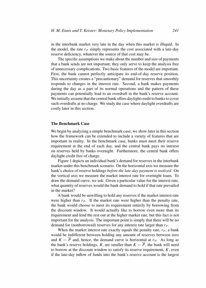
Figure 1 depicts an individual bank’s demand for reserves in the interbankmarket under this benchmark scenario. On the horizontal axis we measure thebank’s choice of reserve holdings before the late-day payment is realized. Onthe vertical axis we measure the market interest rate for overnight loans. Todraw the demand curve, we ask: Given a particular value for the interest rate,what quantity of reserves would the bank demand to hold if that rate prevailedin the market?
A bank would be unwilling to hold any reserves if the market interest ratewere higher than rP . If the market rate were higher than the penalty rate,the bank would choose to meet its requirement entirely by borrowing fromthe discount window. It would actually like to borrow even more than itsrequirement and lend the rest out at the higher market rate, but this fact is notimportant for the analysis. The important point is simply that there will be nodemand for (nonborrowed) reserves for any interest rate larger than rP .
When the market interest rate exactly equals the penalty rate, rP , a bankwould be indifferent between holding any amount of reserves between zeroand K − P and, hence, the demand curve is horizontal at rP . As long asthe bank’s reserve holdings, R, are smaller than K − P , the bank will needto borrow at the discount window to satisfy its reserve requirement, K , evenif the late-day inflow of funds into the bank’s reserve account is the largest

242 Federal Reserve Bank of Richmond Economic Quarterly
Figure 1 Benchmark Demand for Reserves
r
rP
rT
0 K-P K ST
K+P R
Demand for Reserves
possible value, P .7 The alternative would be to borrow more reserves in themarket to reduce this potential need for discount window lending. Since themarket rate is equal to the penalty rate, both strategies deliver the same levelof profit and the bank is indifferent between them.
For market interest rates below the penalty rate, however, a bank willchoose to hold at least K − P reserves. As discussed above, if the bank heldfewer than K − P reserves it would be certain to need to borrow from thediscount window, which would not be an optimal choice when the marketrate is lower than the discount rate. The bank’s demand for reserves in thissituation can be described as “precautionary” in the sense that the bank choosesits reserve holdings to balance the possibility of falling short of the requirementagainst the possibility of ending up with extra reserves in its account at theend of the day.
7 To see this, note that even in the best case scenario the bank will find itself holding R+P
reserves after the arrival of the late-day payment flow. When R < K − P , the bank’s end-of-dayholdings of reserves is insufficient to satisfy its reserve requirement, K , unless it takes a loan atthe discount window.

H. M. Ennis and T. Keister: Monetary Policy Implementation 243
If the market interest rate were very low—close to zero—the opportunitycost of holding reserves would be very small. In this case, the bank wouldhold enough precautionary reserves so that it is virtually certain that unfore-seen movements on its balance sheet will not decrease its reserves below therequired level. In other words, the bank will hold K + P reserves in thiscase. If the market interest rate were exactly zero, there would be no oppor-tunity cost of holding reserves. The demand curve is, therefore, flat along thehorizontal axis after K + P .
In between the two extremes, K −P and K +P , the demand for reserveswill vary inversely with the market interest rate measured on the vertical axis;this portion of the demand curve is represented by the downward-slopingline in Figure 1. The curve is downward-sloping for two reasons. First,the market interest rate represents the opportunity cost of holding reservesovernight. When this rate is lower, finding itself with excess balances is lesscostly for the bank and, hence, the bank is more willing to hold precautionarybalances. Second, when the market rate is lower, the relative cost of having toaccess the discount window is larger, which also tends to increase the bank’sprecautionary demand for reserves.
The linearity of the downward-sloping part of the demand curve resultsfrom the assumption that the late-day payment shock is uniformly distributed.With other probability distributions, the demand curve will be nonlinear, butits basic shape will remain unchanged. In particular, the points where thedemand curve intersects the penalty rate, rP , and the horizontal axis will bethe same for any distribution with support
[−P , P].8
The Equilibrium Interest Rate
Suppose, for the moment, that there is a single bank in the economy. Thenthe demand curve in Figure 1 also represents the total demand for reserves.Let S denote the total supply of reserves in the interbank market, as jointlydetermined by the central bank’s open market operations and autonomousfactors. Then the equilibrium interest rate is determined by the height of thedemand curve at point S. As shown in the diagram, there is a unique level ofreserve supply, ST , that will generate a given target interest rate, rT .
Now suppose there are many banks in the economy, but they are all identi-cal in that they have the same level of required reserves, face the same paymentshock, etc. When there are many banks, the total demand for reserves can befound by simply “adding up” the individual demand curves. For any interest
8 The support of the probability distribution is the set of values of the payment shock thatis assigned positive probability. An explicit formula for the demand curve in the uniform case isderived in Ennis and Weinberg (2007). If the shock instead had an unbounded distribution, suchas the normal distribution used by Whitesell (2006) and others, the demand curve would asymptoteto the penalty rate and the horizontal axis but never intersect them.

244 Federal Reserve Bank of Richmond Economic Quarterly
rate r , total demand is simply the sum of the quantity of reserves demandedby each individual bank.
For presentation purposes, it is useful to look at the average demand forreserves, that is, the total demand divided by the number of banks. Whenall banks are identical, the average demand is exactly equal to the demandof each individual bank. In other words, in the benchmark case where banksare identical, the demand curve in Figure 1 also represents the aggregatedemand for reserves, expressed in per-bank terms. The determination of theequilibrium interest rate then proceeds exactly as in the single-bank case. Inparticular, the market-clearing interest rate will be equal to the target rate, rT ,if and only if reserve supply (expressed in per-bank terms) is equal to ST .
Note that the central bank has two distinct ways in which it can potentiallyaffect the market interest rate: changing the supply of reserves available in themarket and changing (either directly or indirectly) the penalty rate. Suppose,for example, that the central bank wishes to decrease the market interest rate.It could either increase the supply of reserves through open market operations,leading to a movement down the demand curve, or it could decrease the penaltyrate, which would rotate the demand curve downward while leaving the supplyof reserves unchanged. Both policies would cause the market interest rateto fall.
Heterogeneity
While the assumption that all banks are identical was useful for simplifyingthe presentation above, it is clearly a poor representation of reality in mosteconomies. The United States, for example, has thousands of banks and otherdepository institutions that differ dramatically in size, range of activities, etc.We now show how the analysis above changes when there is heterogeneityamong banks and, in particular, how the size distribution of banks might affectthe aggregate demand for reserves.
Each bank still has a demand curve of the form depicted in Figure 1, butnow these curves can be different from each other because banks may havedifferent levels of required reserves, face different distributions of the paymentshock, and/or face different penalty rates. These individual demand curvescan be aggregated exactly as before: For any interest rate r , the total demandfor reserves is simply the sum of the quantity of reserves demanded by eachindividual bank. The aggregate demand curve, expressed in per-bank terms,will again be similar to that presented in Figure 1, with the exact shape beingdetermined by the properties of the various individual demands. If differentbanks have different levels of required reserves, for example, the requirementK in the aggregate demand curve will be equal to the average of the individualbanks’ requirements.
H. M. Ennis and T. Keister: Monetary Policy Implementation 245
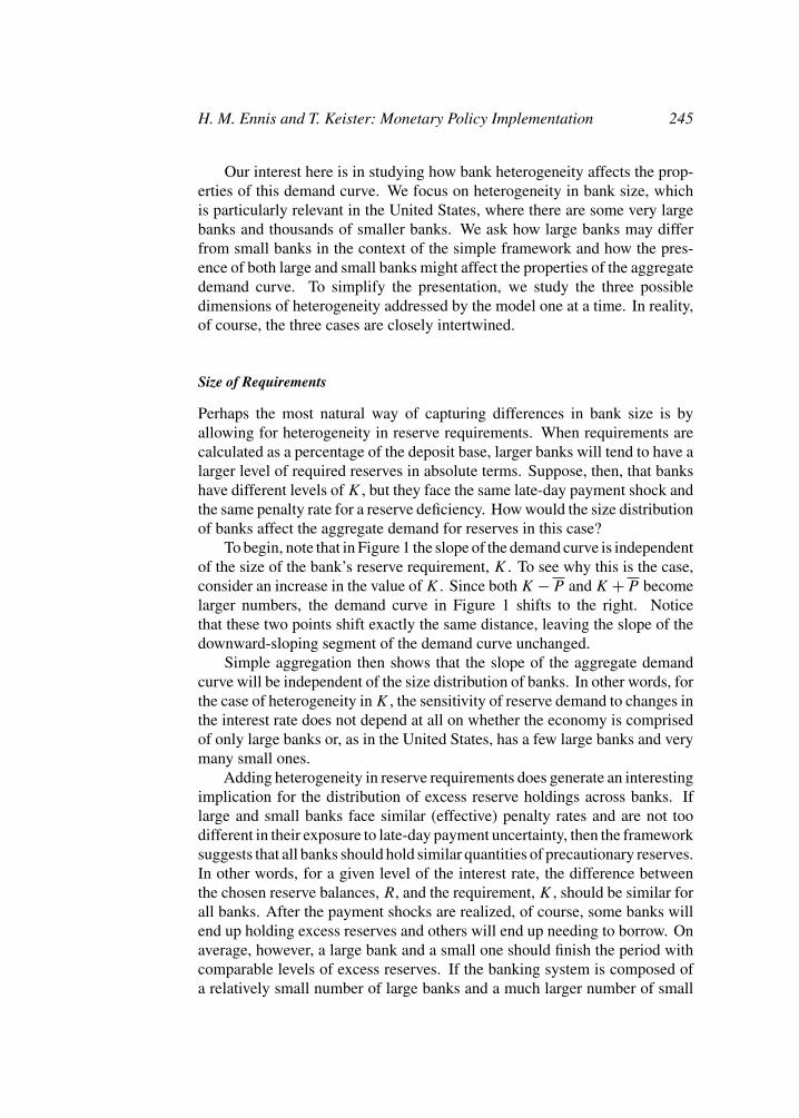
Our interest here is in studying how bank heterogeneity affects the prop-erties of this demand curve. We focus on heterogeneity in bank size, whichis particularly relevant in the United States, where there are some very largebanks and thousands of smaller banks. We ask how large banks may differfrom small banks in the context of the simple framework and how the pres-ence of both large and small banks might affect the properties of the aggregatedemand curve. To simplify the presentation, we study the three possibledimensions of heterogeneity addressed by the model one at a time. In reality,of course, the three cases are closely intertwined.
Size of Requirements
Perhaps the most natural way of capturing differences in bank size is byallowing for heterogeneity in reserve requirements. When requirements arecalculated as a percentage of the deposit base, larger banks will tend to have alarger level of required reserves in absolute terms. Suppose, then, that bankshave different levels of K , but they face the same late-day payment shock andthe same penalty rate for a reserve deficiency. How would the size distributionof banks affect the aggregate demand for reserves in this case?
To begin, note that in Figure 1 the slope of the demand curve is independentof the size of the bank’s reserve requirement, K . To see why this is the case,consider an increase in the value of K . Since both K −P and K +P becomelarger numbers, the demand curve in Figure 1 shifts to the right. Noticethat these two points shift exactly the same distance, leaving the slope of thedownward-sloping segment of the demand curve unchanged.
Simple aggregation then shows that the slope of the aggregate demandcurve will be independent of the size distribution of banks. In other words, forthe case of heterogeneity in K , the sensitivity of reserve demand to changes inthe interest rate does not depend at all on whether the economy is comprisedof only large banks or, as in the United States, has a few large banks and verymany small ones.
Adding heterogeneity in reserve requirements does generate an interestingimplication for the distribution of excess reserve holdings across banks. Iflarge and small banks face similar (effective) penalty rates and are not toodifferent in their exposure to late-day payment uncertainty, then the frameworksuggests that all banks should hold similar quantities of precautionary reserves.In other words, for a given level of the interest rate, the difference betweenthe chosen reserve balances, R, and the requirement, K , should be similar forall banks. After the payment shocks are realized, of course, some banks willend up holding excess reserves and others will end up needing to borrow. Onaverage, however, a large bank and a small one should finish the period withcomparable levels of excess reserves. If the banking system is composed ofa relatively small number of large banks and a much larger number of small
246 Federal Reserve Bank of Richmond Economic Quarterly
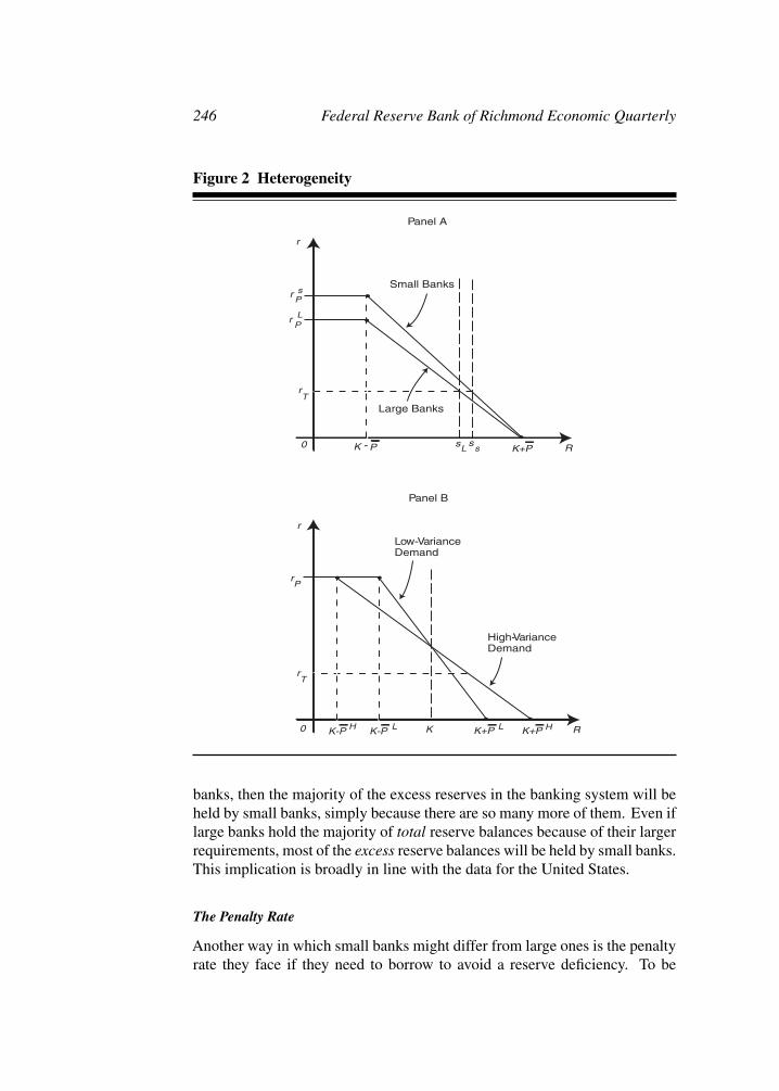
Figure 2 Heterogeneity
Small Banks
Large Banks
Panel A
Panel B
Low-VarianceDemand
High-VarianceDemand
r
r sP
r LP
rT
0 K - P s sL s K+P R
r
r
r
P
T
0 K-P K-P K K+P K+PH HL L R
banks, then the majority of the excess reserves in the banking system will beheld by small banks, simply because there are so many more of them. Even iflarge banks hold the majority of total reserve balances because of their largerrequirements, most of the excess reserve balances will be held by small banks.This implication is broadly in line with the data for the United States.
The Penalty Rate
Another way in which small banks might differ from large ones is the penaltyrate they face if they need to borrow to avoid a reserve deficiency. To be

H. M. Ennis and T. Keister: Monetary Policy Implementation 247
eligible to borrow at the discount window, for example, a bank must establishan agreement with its Reserve Bank and post collateral. This fixed cost maylead some smaller banks to forgo accessing the discount window and insteadborrow at a very high rate in the market (or pay the reserve deficiency fee)when necessary. Smaller banks may also have fewer established relationshipswith counterparties in the fed funds market and, as a consequence, may find itmore difficult to borrow at a favorable interest rate late in the day (seeAshcraft,McAndrews, and Skeie 2007).
Suppose small banks do face a higher penalty rate, such as the value rSP
depicted in Figure 2, Panel A, while larger banks face a lower rate, rLP . The
figure is drawn as if the two banks have the same level of requirements, butthis is done only to make the comparison between the curves clear. The figureshows two immediate implications of this type of heterogeneity. First, atany given interest rate, small banks will hold a higher level of precautionaryreserves, that is, they will choose a larger reserve balance relative to theirlevel of required reserves. In the figure, the smaller bank will hold a quantitySS while the larger bank holds only SL, even though—in this example—bothface the same requirement and the same uncertainty about their end-of-daybalance. As a result, the distribution of excess reserves in the economy willtend to be skewed even more heavily toward small banks than the earlierdiscussion would suggest.
The second implication shown in Figure 2, Panel A is that the demandcurve for small banks has a steeper slope. In an economy with a large numberof small banks, therefore, the aggregate demand curve will tend to be steeper,meaning that average reserve balances will be less sensitive to changes in themarket interest rate. Notice that this result obtains even though there are nocosts of reserve management in the model.
Support of the Payment Shock
A third way in which banks potentially differ from each other is in the distri-bution of the late-day payment shock they face. Figure 2, Panel B depicts twodemand curves, one for a bank facing a higher variance of this distribution andone for a bank facing a lower variance. The figure shows that having moreuncertainty about the end-of-day reserve position leads to a flatter demandcurve and, hence, a reserve balance that is more responsive to changes in theinterest rate.
In this case, it is not completely clear which curve corresponds better tolarge banks and which to small banks. Banks with larger and more complexoperations might be expected to face much larger day-to-day variations intheir payment flows. However, such banks also tend to have sophisticatedreserve management systems in place. As a result, it is not clear whether theend-of-day uncertainty faced by a large bank is higher or lower than that faced

248 Federal Reserve Bank of Richmond Economic Quarterly
by a small bank.9 The effect of the size distribution of banks on the shape ofthe aggregate demand curve is, therefore, ambiguous in this case.
Daylight Credit Fees
So far, we have proceeded under the assumption that banks are free to holdnegative balances in their reserve accounts during the day and that no feesare associated with such daylight overdrafts. Most central banks, however,place some restriction on banks’ access to overdrafts. In many cases, banksmust post collateral at the central bank in order to be allowed to overdraft theiraccount. The Federal Reserve currently charges an explicit fee for daylightoverdrafts to compensate for credit risk. We now investigate how reservedemand changes in the basic framework when access to daylight credit iscostly.
Suppose a bank sends its daytime payment, PD, before receiving the in-coming payment. If PD is larger than R (the bank’s reserve holdings), thebank’s account will be overdrawn until the offsetting payment arrives. Letre denote the interest rate the central bank charges on daylight credit, δ de-note the time period between the two payment flows during the day, and π
denote the probability that a bank sends the outgoing payment before receiv-ing the incoming one. Then the bank’s expected cost of daylight credit isπreδ (PD − R). This expression shows that an additional dollar of reserveholdings will decrease the bank’s expected cost of daylight credit by πreδ.In this way, the terms at which the central bank offers daylight credit caninfluence the bank’s choice of reserve position.10
Figure 3 depicts a bank’s demand for reserves when daylight credit iscostly (that is, when re > 0). The case studied in Figure 1 (that is, whenre = 0) is included in the figure for reference. It is still true that there will beno demand for reserves if the market rate is above the penalty rate rP . Theinterest rate measured on the vertical axis is (as in all of our figures) the ratefor a 24-hour loan. If the market rate were above the penalty rate, a bankwould prefer to lend out all of its reserves at the (high) market rate and satisfyits requirements by borrowing at the penalty rate. By arranging these loans tosettle at approximately the same time on both days, this plan would have no
9 One possibility is that large banks face a wider support of the shock because of their largeroperations, but face a smaller variance because of economies of scale in reserve management. Thisdistinction cannot be captured in the figures here, which are drawn under the assumption that thedistribution of the payment shock is uniform. For other distributions, the variance generally playsa more important role in the analysis than the support.
10 The treatment of overnight reserves can, in turn, influence the level of daylight credit usage.See Ennis and Weinberg (2007) for an investigation of this effect in a closely-related framework.See, also, the discussion in Keister, Martin, and McAndrews (2008).

H. M. Ennis and T. Keister: Monetary Policy Implementation 249
Figure 3 Daylight Credit Fees
r
r
r
r
P
T
e
0 K-P K+PSS P R
Positive Fee
No Fee
effect on the bank’s daylight credit usage and, hence, would generate a pureprofit.
It is also still true that whenever the market rate is below the penaltyrate, the bank will choose to hold at least K − P reserves, since otherwiseit would be certain to need a discount window loan to meet its requirement.As the figure shows, the downward-sloping part of the demand curve is flatterwhen daylight credit is costly. For any market interest rate below the discountrate, the bank will choose to hold a higher quantity of reserves because thesereserves now have the added benefit of reducing daylight credit fees.
Rather than decreasing all the way to the horizontal axis as in Figure 1,the demand curve now becomes flat at the bank’s expected marginal cost ofintraday funds, πreδ. As long as R is smaller than PD, the bank would not bewilling to lend out funds at an interest rate below πreδ, because the expectedincrease in daylight credit fees would be more than the interest earned on theloan. For values of R larger than PD, the bank is holding sufficient reserves tocover all of its intraday payments and the demand curve drops to the horizontalaxis.11
11 The analysis here assumes a particular form of daylight credit usage; if an overdraft occurs,the size of the overdraft is constant over time. Alternative assumptions about the process of daytimepayments would lead to minor changes in the figure, but the qualitative properties would be largely
250 Federal Reserve Bank of Richmond Economic Quarterly
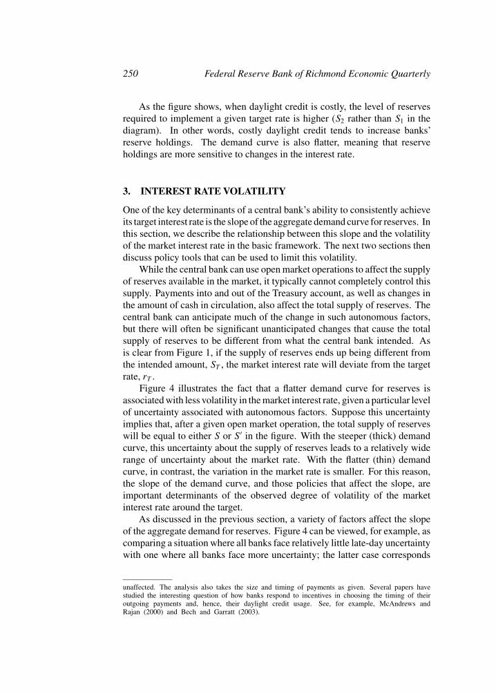
As the figure shows, when daylight credit is costly, the level of reservesrequired to implement a given target rate is higher (S2 rather than S1 in thediagram). In other words, costly daylight credit tends to increase banks’reserve holdings. The demand curve is also flatter, meaning that reserveholdings are more sensitive to changes in the interest rate.
3. INTEREST RATE VOLATILITY
One of the key determinants of a central bank’s ability to consistently achieveits target interest rate is the slope of the aggregate demand curve for reserves. Inthis section, we describe the relationship between this slope and the volatilityof the market interest rate in the basic framework. The next two sections thendiscuss policy tools that can be used to limit this volatility.
While the central bank can use open market operations to affect the supplyof reserves available in the market, it typically cannot completely control thissupply. Payments into and out of the Treasury account, as well as changes inthe amount of cash in circulation, also affect the total supply of reserves. Thecentral bank can anticipate much of the change in such autonomous factors,but there will often be significant unanticipated changes that cause the totalsupply of reserves to be different from what the central bank intended. Asis clear from Figure 1, if the supply of reserves ends up being different fromthe intended amount, ST , the market interest rate will deviate from the targetrate, rT .
Figure 4 illustrates the fact that a flatter demand curve for reserves isassociated with less volatility in the market interest rate, given a particular levelof uncertainty associated with autonomous factors. Suppose this uncertaintyimplies that, after a given open market operation, the total supply of reserveswill be equal to either S or S ′ in the figure. With the steeper (thick) demandcurve, this uncertainty about the supply of reserves leads to a relatively widerange of uncertainty about the market rate. With the flatter (thin) demandcurve, in contrast, the variation in the market rate is smaller. For this reason,the slope of the demand curve, and those policies that affect the slope, areimportant determinants of the observed degree of volatility of the marketinterest rate around the target.
As discussed in the previous section, a variety of factors affect the slopeof the aggregate demand for reserves. Figure 4 can be viewed, for example, ascomparing a situation where all banks face relatively little late-day uncertaintywith one where all banks face more uncertainty; the latter case corresponds
unaffected. The analysis also takes the size and timing of payments as given. Several papers havestudied the interesting question of how banks respond to incentives in choosing the timing of theiroutgoing payments and, hence, their daylight credit usage. See, for example, McAndrews andRajan (2000) and Bech and Garratt (2003).

H. M. Ennis and T. Keister: Monetary Policy Implementation 251
Figure 4 Interest Rate Volatility
Low VolatilityHighVolatility
r
r
r
r
r
P
H
L
L
0 S S R
to the thin line in the figure. However, it should be clear that the reasoningpresented above does not depend on this particular interpretation. The exactsame results about interest rate volatility would obtain if the demand curves haddifferent slopes because banks face different penalty rates in the two scenariosor because of some other factor(s). What the figure shows is that there is adirect relationship between the slope of the demand curve and the amount ofinterest rate volatility caused by forecast errors or other unanticipated changesin the supply of reserves.
Central banks generally aim to limit the volatility of the interest rate aroundtheir target level to the extent possible. For this reason, a variety of policyarrangements have been designed in an attempt to decrease the slope of thedemand curve, at least in the region that is considered “relevant.” In theremainder of the article, we show how some of these tools can be analyzedin the context of our simple framework. In Section 4 we discuss reservemaintenance periods, while in Section 5 we discuss approaches that becomefeasible when the central bank pays interest on reserves.
4. RESERVE MAINTENANCE PERIODS
Perhaps the most significant arrangement designed to flatten the demand curvefor reserves is the introduction of reserve maintenance periods. In a system

252 Federal Reserve Bank of Richmond Economic Quarterly
with a reserve maintenance period, banks are not required to hold a particularquantity of reserves each day. Rather, each bank is required to hold a certainaverage level of reserves over the maintenance period. In the United States,the length of the maintenance period is currently two weeks.
The presence of a reserve maintenance period gives banks some flexibilityin determining when they hold reserves to meet their requirement. In general,banks will try to hold more reserves on days in which they expect the marketinterest rate to be lower and fewer reserves on days when they expect the rateto be higher. This flexibility implies that a bank’s reserve holdings will tend tobe more responsive to changes in the interest rate on any given day. In otherwords, having a reserve maintenance period tends to make the demand curveflatter, at least on days prior to the last day of the maintenance period. Weillustrate this effect by studying a two-day maintenance period in the contextof the simple framework. We then briefly explain how the same logic appliesto longer periods.
A Two-Day Maintenance Period
Let K denote the average daily requirement so that the total requirement forthe two-day maintenance period is 2K . The derivation of the demand curvefor reserves on the second (and final) day of the maintenance period followsexactly the same logic as in our benchmark case. The only difference withFigure 1 is that the reserve requirement will be given by the amount of reservesthat the bank has left to hold in order to satisfy the requirement for the period.In other words, the reserve requirement on the second day is equal to 2K
minus the quantity of reserves the bank held at the end of the first day.On the first day of the maintenance period, a bank’s demand for reserves
depends crucially on its belief about what the market interest rate will be on thesecond day. Suppose the bank expects the market interest rate on the secondday to equal the target rate, rT . Figure 5 depicts the demand for reserves on thefirst day under this assumption.12 As in the basic case presented in Figure 1,there would be no demand for reserves if the market interest rate were greaterthan rP . Suppose instead that the market interest rate on the first day is closeto, but smaller than, the penalty rate, rP . Then the bank will want to satisfy asmuch of its reserve requirement as possible on the second day, when it expectsthe rate to be substantially lower. However, if the bank’s reserve balance afterthe late-day payment shock is negative, it will be forced to borrow funds at thepenalty rate to avoid incurring an overnight overdraft. As long as the marketrate is below the penalty rate, the bank will choose a reserve position of at least−P . Note that this reserve position represents the amount of reserves held by
12 For simplicity, Figure 5 is drawn with no discounting on the part of the bank. The effectof discounting is very small and inessential for understanding the basic logic described here.

H. M. Ennis and T. Keister: Monetary Policy Implementation 253
Figure 5 A Two-Day Maintenance Period
P
T
P P0
r
r
r
2K-P 2K+P R
the bank before the late-day payment shock is realized. Even if this position isnegative, as would be the case when the market rate is close to rP in Figure 5,it is still possible that the bank will receive a late-day inflow of reserves suchthat it does not need to borrow funds at the penalty rate to avoid an overnightoverdraft. However, if the bank were to choose a position smaller than −P ,it would be certain to need to borrow at the penalty rate, which cannot be anoptimal choice as long as the market rate is lower.
For interest rates below rP , but still larger than the target rate, the bank willchoose to hold some “precautionary” reserves to decrease the probability thatit will need to borrow at the penalty rate. This precautionary motive generatesthe first downward-sloping part of the demand curve in the figure. As longas the day-one interest rate is above the target rate, however, the bank willnot hold more than P in reserves on the first day. By holding P , the bank isassured that it will have a positive reserve balance after the late-day paymentshock. If the bank were holding more than P on the first day, it could lendthose reserves out at the (relatively high) market rate and meet its requirementby borrowing reserves on the second day in the event that the interest rate isexpected to be at the (lower) target rate, yielding a positive profit. Hence, thefirst downward-sloping part of the demand curve must end at P .
Now suppose the first-day interest rate is exactly equal to the target rate,rT . In this case, the bank expects the rate to be the same on both days and is,

254 Federal Reserve Bank of Richmond Economic Quarterly
therefore, indifferent between holding reserves on either day for the purposeof meeting reserve requirements. In choosing its first-day reserve position, thebank will consider the following issues. It will choose to hold at least enoughreserves to ensure that it will not need to borrow at the penalty rate at the endof the first day. In other words, reserve holdings will be at least as large as thelargest possible payment P .
The bank is willing to hold more reserves than P for the purpose ofsatisfying some of its requirement. However, it wants to avoid the possi-bility of over-satisfying the requirement on the first day (that is, becoming“locked-in”), since it must hold a non-negative quantity of reserves on thesecond day to avoid an overnight overdraft. This implies that the bank willnot be willing to hold more than the total requirement, 2K , minus the largestpossible payment inflow, P , on the first day. The demand curve is flat betweenthese two points (that is, P and 2K −P ), indicating that the bank is indifferentbetween the various levels of reserves in this interval.
Finally, suppose the market interest rate on the first day is smaller than thetarget rate. Then the bank wants to satisfy most of the requirement on the firstday, since it expects the market rate to be higher on the second day. In this case,the bank will hold at least 2K − P reserves on the first day. If it held any lessthan this amount, it would be certain to have some requirement remaining onthe second day, which would not be an optimal choice given that the rate willbe higher on the second day. As the interest rate moves farther below the targetrate, the bank will hold more reserves for the usual precautionary reasons. Inthis case, the bank is balancing the possibility of being locked-in after thefirst day against the possibility of needing to meet some of its requirement onthe more-expensive second day. The larger the difference between the rateson the two days, the larger the quantity the bank will choose to hold on thefirst day. This trade-off generates the second downward-sloping part of thedemand curve.
The intermediate flat portion of the demand curve in Figure 5 can helpto reduce the volatility of the interest rate on days prior to the settlementday. As long as movements in autonomous factors are small enough such thatthe supply of reserves stays in this portion of the demand curve, interest ratefluctuations will be minimal. For a central bank that is interested in minimizingvolatility around its target rate, this represents a substantial improvement overthe situation depicted in Figure 1.13
13 It should be noted that Figure 5 is drawn under the assumption that the reserve requirementis relatively large. Specifically, K > P is assumed to hold, so that the total reserve requirement forthe period, 2K , is larger than the width of the support of the late-day payment shock, 2P . If thisinequality were reserved, the flat portion of the demand curve would not exist. In general, reservemaintenance periods are most useful as a policy tool when the underlying reserve requirementsare sufficiently large relative to the end-of-day balance uncertainty.
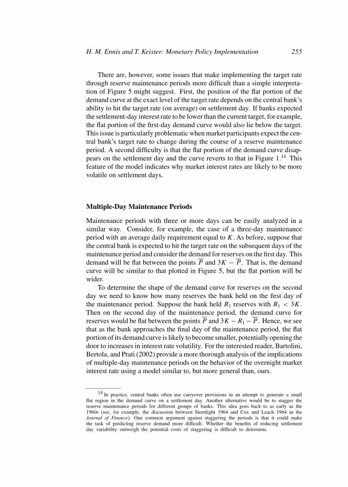
H. M. Ennis and T. Keister: Monetary Policy Implementation 255
There are, however, some issues that make implementing the target ratethrough reserve maintenance periods more difficult than a simple interpreta-tion of Figure 5 might suggest. First, the position of the flat portion of thedemand curve at the exact level of the target rate depends on the central bank’sability to hit the target rate (on average) on settlement day. If banks expectedthe settlement-day interest rate to be lower than the current target, for example,the flat portion of the first-day demand curve would also lie below the target.This issue is particularly problematic when market participants expect the cen-tral bank’s target rate to change during the course of a reserve maintenanceperiod. A second difficulty is that the flat portion of the demand curve disap-pears on the settlement day and the curve reverts to that in Figure 1.14 Thisfeature of the model indicates why market interest rates are likely to be morevolatile on settlement days.
Multiple-Day Maintenance Periods
Maintenance periods with three or more days can be easily analyzed in asimilar way. Consider, for example, the case of a three-day maintenanceperiod with an average daily requirement equal to K. As before, suppose thatthe central bank is expected to hit the target rate on the subsequent days of themaintenance period and consider the demand for reserves on the first day. Thisdemand will be flat between the points P and 3K − P . That is, the demandcurve will be similar to that plotted in Figure 5, but the flat portion will bewider.
To determine the shape of the demand curve for reserves on the secondday we need to know how many reserves the bank held on the first day ofthe maintenance period. Suppose the bank held R1 reserves with R1 < 3K .Then on the second day of the maintenance period, the demand curve forreserves would be flat between the points P and 3K −R1 −P . Hence, we seethat as the bank approaches the final day of the maintenance period, the flatportion of its demand curve is likely to become smaller, potentially opening thedoor to increases in interest rate volatility. For the interested reader, Bartolini,Bertola, and Prati (2002) provide a more thorough analysis of the implicationsof multiple-day maintenance periods on the behavior of the overnight marketinterest rate using a model similar to, but more general than, ours.
14 In practice, central banks often use carryover provisions in an attempt to generate a smallflat region in the demand curve on a settlement day. Another alternative would be to stagger thereserve maintenance periods for different groups of banks. This idea goes back to as early as the1960s (see, for example, the discussion between Sternlight 1964 and Cox and Leach 1964 in theJournal of Finance). One common argument against staggering the periods is that it could makethe task of predicting reserve demand more difficult. Whether the benefits of reducing settlementday variability outweigh the potential costs of staggering is difficult to determine.
256 Federal Reserve Bank of Richmond Economic Quarterly
5. PAYING INTEREST ON RESERVES
We now introduce the possibility that the central bank pays interest on thereserve balances held overnight by banks in their accounts at the central bank.As discussed in Section 1, most central banks currently pay interest on reservesin some form, and Congress has authorized the Federal Reserve to begin doingso in October 2011. The ability to pay interest on reserves gives a central bankan additional policy tool that can be used to help minimize the volatility ofthe market interest rate and steer this rate to the target level. This tool can beespecially useful during periods of financial distress. For example, during therecent financial turmoil, the fed funds rate has experienced increased volatilityduring the day and has, in many cases, collapsed to values near zero late inthe day. As we will see below, the ability to pay interest on reserves allowsthe central bank to effectively put a floor on the values of the interest rate thatcan be observed in the market. Such a floor reduces volatility and potentiallyincreases the ability of the central bank to achieve its target rate.
In this section, we describe two approaches to monetary policy imple-mentation that rely on paying interest on reserves: an interest rate corridorand a system with clearing bands. We explain the basic components of eachapproach and how each tends to flatten the demand curve for reserves.
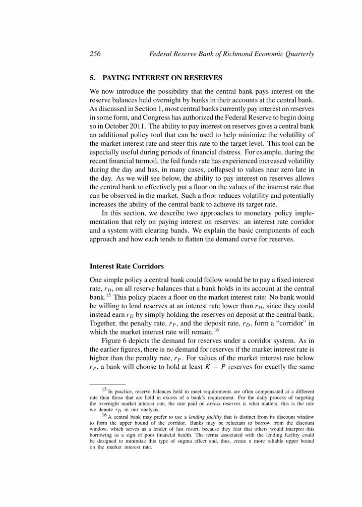
Interest Rate Corridors
One simple policy a central bank could follow would be to pay a fixed interestrate, rD, on all reserve balances that a bank holds in its account at the centralbank.15 This policy places a floor on the market interest rate: No bank wouldbe willing to lend reserves at an interest rate lower than rD, since they couldinstead earn rD by simply holding the reserves on deposit at the central bank.Together, the penalty rate, rP , and the deposit rate, rD, form a “corridor” inwhich the market interest rate will remain.16
Figure 6 depicts the demand for reserves under a corridor system. As inthe earlier figures, there is no demand for reserves if the market interest rate ishigher than the penalty rate, rP . For values of the market interest rate belowrP , a bank will choose to hold at least K − P reserves for exactly the same
15 In practice, reserve balances held to meet requirements are often compensated at a differentrate than those that are held in excess of a bank’s requirement. For the daily process of targetingthe overnight market interest rate, the rate paid on excess reserves is what matters; this is the ratewe denote rD in our analysis.
16 A central bank may prefer to use a lending facility that is distinct from its discount windowto form the upper bound of the corridor. Banks may be reluctant to borrow from the discountwindow, which serves as a lender of last resort, because they fear that others would interpret thisborrowing as a sign of poor financial health. The terms associated with the lending facility couldbe designed to minimize this type of stigma effect and, thus, create a more reliable upper boundon the market interest rate.

H. M. Ennis and T. Keister: Monetary Policy Implementation 257
Figure 6 A Conventional Corridor
r
r
r
r
P
T
D
0 K-P K ST K+P R
Demand forReserves
reason as in Figure 1: if it held a lower level of reserves, it would be certain toneed to borrow at the penalty rate, rP . Also as before, the demand for reservesis downward-sloping in this region. The big change from Figure 1 is that thedemand curve now becomes flat at the deposit rate. If the market rate werelower than the deposit rate, a bank’s demand for reserves would be essentiallyinfinite, as it would try to borrow at the market rate and earn a profit by simplyholding the reserves overnight.
The figure shows that, regardless of the level of reserve supply, S, themarket interest rate will always stay in the corridor formed by the rates rP
and rD. The width of the corridor, rP − rD, is then a policy choice. Choosinga relatively narrow corridor will clearly limit the range and volatility of themarket interest rate. Note that narrowing the corridor also implies that thedownward-sloping part of the demand curve becomes flatter (to see this, noticethat the boundary points K − P and K + P do not depend on rP or rD).Hence, the size of the interest rate movement associated with a given shockto an autonomous factor is smaller, even when the shock is small enough tokeep the rate within the corridor.
An interesting case to consider is one in which the lending and depositrates are set the same distance on either side of the target rate (x basis pointsabove and below the target, respectively). This system is called a symmetric
258 Federal Reserve Bank of Richmond Economic Quarterly
corridor. A change in policy stance that involves increasing the target rate,then, effectively amounts to changing the levels of the lending and depositrates, which shifts the demand curve along with them. The supply of reservesneeded to maintain a higher target rate, for example, may not be lower. Infact— perhaps surprisingly—in the simple model studied here, the target levelof the supply of reserves would not change at all when the policy rate changes.
If the demand curve in Figure 6 is too steep to allow the central bank toeffectively achieve its goal of keeping the market rate close to the target, acorridor system could be combined with a reserve maintenance period of thetype described in Section 4. The presence of a reserve maintenance periodwould generate a flat region in the demand curve as in Figure 5. The features ofthe corridor would make the two downward-sloping parts of the demand curvein Figure 5 less steep, which would limit the interest rate volatility associatedwith events where reserve supply exits the flat region of the demand curve, aswell as on the last day of the maintenance period when the flat region is notpresent.
Another way to limit interest rate volatility is for the central bank to set thedeposit rate equal to the target rate and then provide enough reserves to makethe supply, ST , intersect the demand curve well into the flat portion of thedemand curve at rate rD. This “floor system” has been recently advocated as away to simplify monetary policy implementation (see, for example, Woodford2000, Goodfriend 2002, and Lacker 2006). Note that such a system doesnot rely on a reserve maintenance period to generate the flat region of thedemand curve, nor does it rely on reserve requirements to induce banks tohold reserves. To the extent that reserve requirements, and the associatedreporting procedures, place significant administrative burdens on both banksand the central bank, setting the floor of the corridor at the target rate andsimplifying, or even eliminating, reserve requirements could potentially be anattractive system for monetary policy implementation.
It should be noted, however, that the market interest rate will alwaysremain some distance above the floor in such a system, since lenders in themarket must be compensated for transactions costs and for assuming somecounterparty credit risk. In other words, in a floor system the central bank isable to fully control the risk-free interest rate, but not necessarily the marketrate. In normal times, the gap between the market rate and the rate paid onreserves would likely be stable and small. In periods of financial distress,however, elevated credit risk premia may drive the average market interestrate significantly above the interest rate paid on reserves. Our simple modelabstracts from these important considerations.17
17 The central bank could also set an upper limit for the quantity of reserves on which itwould pay the target rate of interest to a bank; reserves above this limit would earn a lowerrate (possibly zero). Whitesell (2006) proposed that banks be allowed to choose their own upper

H. M. Ennis and T. Keister: Monetary Policy Implementation 259
Clearing Bands
Another approach to generating a flat region in the demand curve for re-serves is the use of daily clearing bands. This approach does not rely on areserve maintenance period. Instead, the central bank pays interest on a bank’sreserve holdings at the target rate, rT , as long as those holdings fall within apre-specified band. Let K and K denote the lower and upper bounds of thisband, respectively. If the bank’s reserve balance falls below K , it must borrowat the penalty rate, rP , to bring its balance up to at least K . If, on the otherhand, the bank’s reserve balance is higher than K , it will earn the target rate,rT , on all balances up to K but will earn a lower rate, rE , beyond that bound.
The demand curve for reserves under such a system is depicted in Figure7. The figure is drawn under the assumption that the clearing band is fairlywide relative to the support of the late-day payment shock. In particular, weassume that K + P < K − P . Let us call the interval
[K + P , K − P
]the
“intermediate region” for reserves. By choosing any level of reserves in thisintermediate region, a bank can ensure that its end-of-day reserve balance willfall within the clearing band. The bank would then be sure that it will earn thetarget rate of interest on all of the reserves it ends up holding overnight.
When the market interest rate is equal to the target rate, rT , a bank isindifferent between choosing any level of reserves in the intermediate region.For example, if the bank borrows in the market to slightly increase its reserveholdings, the cost it would pay in the market for those reserves would be exactlyoffset by the extra interest it would earn from the central bank. Similarly,lending out reserves to slightly decrease the bank’s holdings would also leaveprofit unchanged. This reasoning shows that the demand curve for reserveswill be flat in the intermediate region between K + P and K − P . As long asthe central bank is able to keep the supply of reserves within this region, themarket interest rate will equal the target rate, rT , regardless of the exact levelof reserve supply.
Outside the intermediate region, the logic behind the shape of the demandcurve is very similar to that explained in our benchmark case. When the marketinterest rate is higher than rT , a bank can earn more by lending reserves inthe market than by holding them on deposit at the central bank. It would,therefore, prefer not to hold more than the minimum level of reserves neededto avoid being penalized, K . Of course, the bank would be willing to holdsome precautionary reserves to guard against the possibility that the late-day payment shock will drive their reserve balance below K . The quantity ofprecautionary reserves it would choose to hold is, as before, an inverse functionof the market interest rate; this reasoning generates the first downward-slopingpart of the demand curve in Figure 7.
limits by paying a facility fee per unit of capacity. Such an approach leads to a demand curvefor reserves that is flat at the target rate over a wide region.

260 Federal Reserve Bank of Richmond Economic Quarterly
Figure 7 A Clearing Band
r
rP
rT
rE
0 K-P K-PK+P K+P R
When the market rate is below rT , on the other hand, the bank would liketo take full advantage of its ability to earn the target interest rate by holdingreserves at the central bank. It would, however, take into consideration thepossibility that a late-day inflow of funds will leave it with a final balancehigher than K , in which case it would earn the lower interest rate, rE , on theexcess funds. The resulting decision process generates a downward-slopingregion of the demand curve between the rates rT and rE . As in Figure 6, thedemand curve never falls below the interest rate paid on excess reserves (nowlabeled rE); thus, this rate creates a floor for the market interest rate.
The demand curve in Figure 7 has the same basic shape as the one gen-erated by a reserve maintenance period, which was depicted in Figure 5. It isimportant to keep in mind, however, that the forces generating the flat portionof the demand curve in the intermediate region are fundamentally different inthe two cases. The reserve maintenance period approach relies on intertem-poral arbitrage: banks will want to hold more reserves on days when themarket interest rate is low and fewer reserves when the market rate is high.This activity will tend to equate the current market interest rate to the expectedfuture rate (as long as the supply of reserves is in the intermediate region).The clearing band system relies instead on intraday arbitrage to generate theflat portion of the demand curve: banks will want to hold more reserves when

H. M. Ennis and T. Keister: Monetary Policy Implementation 261
the market interest rate is low, for example, simply to earn the higher interestrate paid by the central bank.
The intertemporal aspect of reserve maintenance periods has two cleardrawbacks. First, if—for whatever reason—the expected future rate differsfrom the target rate, rT , it becomes difficult for the central bank to achieve thetarget rate in the current period. Second, large shocks to the supply of reserveson one day can have spillover effects on subsequent days in the maintenanceperiod. If, for example, the supply of reserves is unusually high one day, bankswill satisfy an unusually large portion of their reserve requirements and, as aresult, the flat portion of the demand curve will be smaller on all subsequentdays, increasing the potential for rate volatility on those days.
The clearing band approach, in contrast, generates a flat portion in thedemand curve that always lies at the current target interest rate, even if marketparticipants expect the target rate to change in the near future. Moreover,the width of the flat portion is “reset” every day; it does not depend on pastevents. These features are important potential advantages of the clearing bandapproach. We should again point out, however, that our simple model hasabstracted from transaction costs and credit risk. As with the floor system dis-cussed above, these considerations could result in the average market interestrate being higher than the rate rT , as the latter represents a risk-free rate.
6. CONCLUSION
A recent change in legislation that allows the Federal Reserve to pay interest onreserves has renewed interest in the debate over the most effective way to im-plement monetary policy. In this article, we have provided a basic frameworkthat can be useful for analyzing the main properties of the various alterna-tives. While we have conducted all our analysis graphically, our simplifyingassumptions permit a fairly precise description of the alternatives and theireffectiveness at implementing a target interest rate.
Many extensions of our basic framework are possible and we have ana-lyzed several of them in this article. However, some important issues remainunexplored. For example, we only briefly mentioned the difficulties that fluc-tuations in aggregate credit risk can introduce in the implementation process.Also, as the debate continues, new questions will arise. We believe that theframework introduced in this article can be a useful first step in the search formuch-needed answers.

262 Federal Reserve Bank of Richmond Economic Quarterly
REFERENCES
Ashcraft, Adam, James McAndrews, and David Skeie. 2007. “PrecautionaryReserves and the Interbank Market.” Mimeo, Federal Reserve Bank ofNew York (July).
Bartolini, Leonardo, Giuseppe Bertola, and Alessandro Prati. 2002.“Day-To-Day Monetary Policy and the Volatility of the Federal FundsInterest Rate.” Journal of Money, Credit, and Banking 34 (February):137–59.
Bech, M. L., and Rod Garratt. 2003. “The Intraday Liquidity ManagementGame.” Journal of Economic Theory 109 (April): 198–219.
Clouse, James A., and James P. Dow, Jr. 2002. “A Computational Model ofBanks’ Optimal Reserve Management Policy.” Journal of EconomicDynamics and Control 26 (September): 1787–814.
Cox, Albert H., Jr., and Ralph F. Leach. 1964. “Open Market Operations andReserve Settlement Periods: A Proposed Experiment.” Journal ofFinance 19 (September): 534–9.
Coy, Peter. 2007. “A ‘Stealth Easing’ by the Fed?” BusinessWeek.http://www.businessweek.com/investor/content/aug2007/pi20070817 445336.htm [17 August].
Dotsey, Michael. 1991. “Monetary Policy and Operating Procedures in NewZealand.” Federal Reserve Bank of Richmond Economic Review(September/October): 13–9.
Ennis, Huberto M., and John A. Weinberg. 2007. “Interest on Reserves andDaylight Credit.” Federal Reserve Bank of Richmond EconomicQuarterly 93 (Spring): 111–42.
Goodfriend, Marvin. 2002. “Interest on Reserves and Monetary Policy.”Federal Reserve Bank of New York Economic Policy Review 8 (May):77–84.
Guthrie, Graeme, and Julian Wright. 2000. “Open Mouth Operations.”Journal of Monetary Economics 46 (October): 489–516.
Hilton, Spence, and Warren B. Hrung. 2007. “Reserve Levels and IntradayFederal Funds Rate Behavior.” Federal Reserve Bank of New York StaffReport 284 (May).
Keister, Todd, Antoine Martin, and James McAndrews. 2008. “DivorcingMoney from Monetary Policy.” Federal Reserve Bank of New YorkEconomic Policy Review 14 (September): 41–56.
H. M. Ennis and T. Keister: Monetary Policy Implementation 263
Lacker, Jeffrey M. 2006. “Central Bank Credit in the Theory of Money andPayments.” Speech. http://www.richmondfed.org/news and speeches/presidents speeches/index.cfm/2006/id=88/pdf=true.
McAndrews, James, and Samira Rajan. 2000. “The Timing and Funding ofFedwire Funds Transfers.” Federal Reserve Bank of New YorkEconomic Policy Review 6 (July): 17–32.
Poole, William. 1968. “Commercial Bank Reserve Management in aStochastic Model: Implications for Monetary Policy.” Journal ofFinance 23 (December): 769–91.
Sternlight, Peter D. 1964. “Reserve Settlement Periods of Member Banks:Comment.” Journal of Finance 19 (March): 94–8.
Whitesell, William. 2006. “Interest Rate Corridors and Reserves.” Journal ofMonetary Economics 53 (September): 1177–95.
Woodford, Michael. 2000. “Monetary Policy in a World Without Money.”International Finance 3 (July): 229–60.
