understanding long range memory effects in deep neural
TRANSCRIPT

arX
iv:2
105.
0206
2v4
[cs
.LG
] 2
8 Ju
n 20
21IEEE TRANSACTIONS ON NEURAL NETWORKS AND LEARNING SYSTEMS 1
Understanding Short-Range Memory Effects in
Deep Neural NetworksChengli Tan, Jiangshe Zhang, and Junmin Liu
Abstract—Stochastic gradient descent (SGD) is of fundamentalimportance in deep learning. Despite its simplicity, elucidating itsefficacy remains challenging. Conventionally, the success of SGDis ascribed to the stochastic gradient noise (SGN) incurred inthe training process. Based on this consensus, SGD is frequentlytreated and analyzed as the Euler-Maruyama discretizationof stochastic differential equations (SDEs) driven by eitherBrownian or Lévy stable motion. In this study, we argue thatSGN is neither Gaussian nor Lévy stable. Instead, inspiredby the short-range correlation emerging in the SGN series,we propose that SGD can be viewed as a discretization of anSDE driven by fractional Brownian motion (FBM). Accordingly,the different convergence behavior of SGD dynamics is well-grounded. Moreover, the first passage time of an SDE drivenby FBM is approximately derived. The result suggests a lowerescaping rate for a larger Hurst parameter, and thus SGDstays longer in flat minima. This happens to coincide withthe well-known phenomenon that SGD favors flat minima thatgeneralize well. Extensive experiments are conducted to validateour conjecture, and it is demonstrated that short-range memoryeffects persist across various model architectures, datasets, andtraining strategies. Our study opens up a new perspective andmay contribute to a better understanding of SGD.
Index Terms—Stochastic gradient descent, deep neural net-works, fractional Brownian motion, first passage time, short-range memory effects.
I. INTRODUCTION
DESPITE the great uncertainty of stochastic processes that
widely occur in nature, it is recognized that they have
memories as well. In the early 1950s, considering regular
floods and irregular flows, which were a severe impediment to
development, the Egyptian government decided to construct a
series of dams and reservoirs to control the Nile. To devise
a method of water control, several hydrologists examined
the rain and drought volatility of the Nile and discovered
a short-range relationship therein [1], [2]. This implies that,
contrary to the common independence assumption, there is
non-negligible dependence between the present and the past.
Determining the behavior and predictability of stochastic
systems is critical to understanding, for example, climate
change [3], financial market [4], and network traffic [5], [6].
Accordingly, it is natural to ask whether or not similar memory
effects exist in deep neural networks (DNNs), which can be
seen as complex stochastic systems.
This work was supported by the National Key Research and DevelopmentProgram of China under Grant 2020AAA0105601 and by the National NaturalScience Foundation of China under Grants 61976174, 61877049.
The authors are with the School of Mathematics and Statistics, Xi’anJiaotong University, Xi’an 710049, China.
Generally, many tasks in DNNs can be reduced to solving
the following unconstrained optimization problem
minw∈Rd
f(w) =1
N
N∑
i=1
fi(w), (1)
where w ∈ Rd represents the weights of the neural network, f
represents the loss function, which is typically non-convex in
w, and each i ∈ 1, 2, · · · , N corresponds to an instance
tuple (xi, yi) of the training samples. Due to the limited
resources and their remarkable inefficiency, deterministic op-
timization algorithms, such as gradient descent (GD), cannot
easily train models with millions of parameters. Instead, in
practice, stochastic optimization approaches, such as SGD and
its variants AdaGrad [7] and Adam [8], are employed. The
SGD recursion process is defined as
wk+1 = wk − η∇f(wk), (2)
where k denotes the kth step, η is the learning rate, and
∇f(wk) is the estimation of the true gradient at the current
step, which is given by
∇f(wk) =1
n
∑
i∈Sk
∇fi(wk). (3)
Here Sk is an index set of a batch of samples independently
drawn from the training dataset S, and n = |Sk| denotes the
cardinality of Sk.
Despite being overwhelmingly over-parameterized, SGD
prevents DNNs from converging to local minima that cannot
generalize well [9]–[13]. One point of view is that SGD
induces implicit regularization by incurring SGN during the
training process [14], which is defined as
νk = ∇f(wk)−∇f(wk), (4)
where ∇f(wk) represents the gradient of the loss function
over the full training dataset S
∇f(wk) =1
N
N∑
i=1
∇fi(wk). (5)
This claim is supported by several observations found in
numerous experiments:
1) SGD generally outperforms GD [13];
2) SGD using large batch size often leads to performance
deterioration compared with SGD using small batch size
[12], [15]–[17];
3) SGD approximations are not as effective as SGD, even
if they are tuned to the same noise intensity [13].
IEEE TRANSACTIONS ON NEURAL NETWORKS AND LEARNING SYSTEMS 2
The first observation confirms that the existence of SGN
is a requisite for models to avoid getting trapped in subopti-
mal points. The second observation indicates that the model
performance is heavily influenced by the noise intensity. The
last observation further implies that the model performance is
affected not only by the noise intensity, but also by the noise
shape. It should be clarified that SGN arises in the process
of batch sampling, which is the major source of randomness,
except for weight initialization and dropout operations. Let
∇f(wk) =1
N∇fk · , (6)
where ∇fk = (∇f1(wk), · · · ,∇fN(wk)) ∈ Rd×N , ∈ R
N
is a random vector, indicating which samples are selected at
the kth iteration. Let 1 be the matrix the elements of which
are equal to 1; then, we can define the sampling noise as
ζ = 1N (− 1). The properties of ζ are given as follows [18]:
1) For a batch sampled without replacement, the SGD
sampling noise ζ satisfies
E [ζ] = 0, Var [ζ] =N − n
nN(N − 1)
(I− 1
N11T
), (7)
2) For a batch sampled with replacement, the SGD sampling
noise ζ satisfies
E [ζ] = 0, Var [ζ] =1
nN
(I− 1
N11T
). (8)
Here I ∈ RN×N is an identity matrix.
From the perspective of sampling noise, the SGN νk is
equivalent to the product of the gradient matrix ∇f(wk) and
the corresponding sampling noise ζ, i.e.,
νk = ∇f(wk)−∇f(wk) = ∇fk · ζ. (9)
Therefore, the first two moments of νk are given by
E [νk] = ∇fk · E [ζ] = 0, (10)
and
Var [νk] = ∇fkVar [ζ]∇fTk , Σk. (11)
It is noteworthy that although the sampling noise is time-
independent, the SGN is deeply affected by the present pa-
rameter state.
A popular approach to studying the behavior of SGN is to
view SGD as a discretization of SDEs [12], [19]–[22]. This
approach relies on the assumption that if the batch size |Sk| is
sufficiently large, then by invoking the central limiting theorem
(CLT), the SGN follows a Gaussian distribution
νk ∼ N (0,Σk). (12)
Based on this assumption, (2) can be translated into
wk+1 = wk − η∇f (wk) + ηνk. (13)
If the learning rate η is sufficiently small to be treated
as a time increment, (13) implements an Euler-Maruyama
approximation of the following Itô process [12]
dwt = −∇f (wt) dt+√ηRkdBt, (14)
where RkRTk = Σk and Bt is the standard Brownian motion.
Following this line, He et al. [17] argued that the generalization
gap is governed by the ratio of the learning rate to the batch
size, which directly controls the intensity of SGN. Further,
they related this ratio to the flatness of minima obtained by
SGD [9], [23]–[25], and concluded that a larger ratio implies
that the minima are wider and thus generalize better. Another
striking perspective is that SGD simulates a Markovian chain
with a stationary distribution [19]. Under certain condition that
the loss function can be well approximated by a quadratic
function, SGD can be used as an approximate Bayesian
posterior inference algorithm. It follows that SGD can be
viewed as a discretization of the continuous-time Ornstein–
Uhlenbeck (OU) process [19]
dwt = −ηAwtdt+η√nBdBt, (15)
which has the following analytic stationary distribution
q(w) ∝ exp
−1
2wTΣ−1w
, (16)
where A,B,Σ satisfy
ΣA+AΣ =η
nBBT . (17)
Furthermore, it was recently argued that the critical as-
sumption that SGN follows a Gaussian distribution does not
necessarily hold [26], [27]. Instead, it was assumed that
the second moment of SGN may not be finite, and it was
concluded that the noise follows a Lévy random process by
invoking the generalized CLT. Therefore, it was proposed that
SGD can be modeled as a Lévy-driven SDE [26]
dwt = −∇f (wt) dt+ η(α−1)/ασ(t, wt)dLαt , (18)
where Lαt denotes the d-dimensional α-stable Lévy motion
with independent components. When α = 2, (18) reduces to
a standard SDE driven by Brownian motion. It was argued
that when α < 2, Lévy-driven GD dynamics require only
polynomial time to transit to another minimum (rather than
exponential time, as in Brownian motion-driven GD dynamics)
because the process can incur discontinuities, and thus the
algorithm can directly jump out.
Instead of focusing on the influence of noise intensity and
noise class, Zhu et al. [13] studied noise shape, namely,
the covariance structure. According to the classical statistical
theory [28], there is an exact equivalence between the Hessian
matrix of the loss and the Fisher information matrix, namely,
the covariance at the optimum. Practically, when the present
parameter is around the true value, the Fisher matrix is close
to the Hessian. Owing to the dominance of noise in the
later stages of SGD iteration [29], the gradient covariance is
approximately equal to the Hessian. Although this is disputable
[30], it is widely appreciated that SGD favors flat minima,
where the spectrum of the Hessian matrix is relatively small.
By measuring the alignment of the noise covariance and the
Hessian matrix of the loss function, it was concluded that
anisotropic noise is superior to isotropic noise in terms of
jumping out of sharp minima. More recently, based on the
assumption that SGN follows a Gaussian distribution, Xie et
al. [31] further derived the mean escaping time of Kramers

IEEE TRANSACTIONS ON NEURAL NETWORKS AND LEARNING SYSTEMS 3
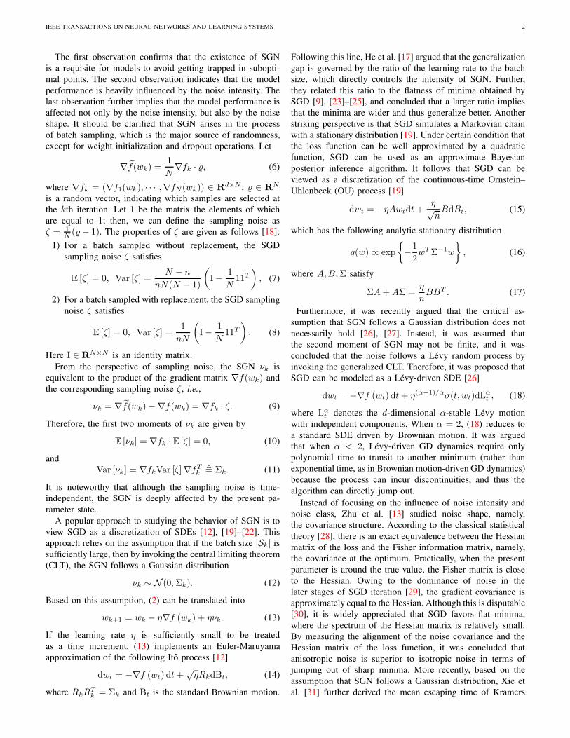
(a) Batch Size = 64 (b) Batch Size = 512
Fig. 1: Local trajectories of SGN mapped onto two-dimensional space for different batch sizes. In both cases, the noise is
generated from the last iteration, and two adjacent dimensions are bound together to plot one trajectory line. The starting point
is uniformly sampled in [0, 1]. Trajectories that resemble lines indicate that the noise in one of the two dimensions is near
zero. The red empty circle indicates the starting point of the trajectory, whereas the blue circle indicates the ending point of
the trajectory.
problem and found that SGD favors flat minima exponentially
more than sharp minima.
A. Issues
Although the aforementioned studies have confirmed the
vitality of SGN, a satisfactory understanding of the full SGD
dynamics is lacking. Several relevant issues are explained in
detail below.
The first issue relates to the infiniteness of the second
moment of SGN, as assumed in [26], [27]. According to
(11), the noise covariance Σk is the product of the sampling
noise and the gradient matrix. Given the precondition that the
covariance of the sampling noise ζ is finite, (11) implies that
whether or not the noise covariance Σk is finite depends solely
on the gradient matrix ∇fk. The main components of DNNs,
such as matrix and convolution operations, are twice differ-
entiable almost everywhere. In addition, common techniques
in deep learning, such as batch normalization [32], near-zero
initialization [33], and gradient clipping [34], ensure that the
parameters will not excessively drift from their initialization.
Hence, it is reasonable to assume that the gradient matrix lies
in a bounded region of interest, and the finiteness of the noise
covariance is ensured. Thus, the assumption that SGN follows
a Lévy stable distribution might be flawed.
The second issue involves the normality of SGN. Although
the second moment of SGN is finite, in practice, it remains
unclear whether the batch size is sufficiently large to ensure
that the normality assumption holds. To this end, Panigrahi et
al. [35] directly conducted Shapiro and Anderson normality
tests on SGN. The results suggest that SGN is highly non-
Gaussian and follows a Gaussian distribution only in the early
training stage for batch sizes of 256 and above.
B. Contributions
Traditionally, we assume that SGN is independently gener-
ated at different iterations, or nearly so. Fig. 1 shows the two-
dimensional trajectories of SGN of the training process for
different batch sizes. It can be observed that the patterns are
disparate, and the trajectories in Fig. 1(a) are almost smooth
and regular, whereas the trajectories in Fig. 1(b) are fractal-
like and exhibit rapid mutations. This raises the question of
whether there exists strong inter-dependence between the SGN
series.
One important class of stochastic processes to characterize
the inter-dependence of economic data is known as FBM.
Bearing the observation in mind that the self-similar sample
paths of FBM are fractals, in this study, we leverage FBM
to study the inter-dependence of the SGN series. Instead of
assuming that SGN is Gaussian or follows a Lévy random
process, we hypothesize that it is generated by FBM, the
increments of which are fractional Gaussian noise (FGN)
and time-dependent. Using the same rationale as in (14) and
(18), we reformulate the SGD dynamics as a discretization
of an FBM-driven SDE. According to the values of the
Hurst parameter, FBM can be classified as super-diffusive
(0.5 < H < 1), sub-diffusive (0 < H < 0.5), and normal-
diffusive (H = 0.5). Therefore, an FBM-driven SDE exhibits
a fundamentally different behavior from that of an ordinary
SDE driven by Brownian motion. As described in Section
III, the convergence rate of an FBM-driven SDE is closely
related to the Hurst parameter; this accounts for the different
convergence behaviors in the SGD training process. When the
training process gets trapped in local minima, we further study
the escaping efficiency from the perspective of the first passage
time of an FBM-driven SDE.
In general, the contributions of this study are the following:
IEEE TRANSACTIONS ON NEURAL NETWORKS AND LEARNING SYSTEMS 4
H = 0.3
H = 0.5
H = 0.7
H = 0.3
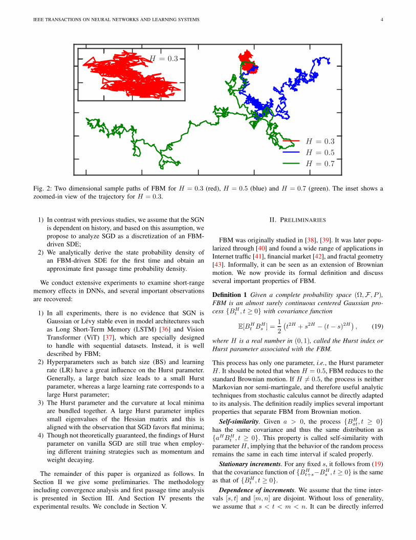
Fig. 2: Two dimensional sample paths of FBM for H = 0.3 (red), H = 0.5 (blue) and H = 0.7 (green). The inset shows a
zoomed-in view of the trajectory for H = 0.3.
1) In contrast with previous studies, we assume that the SGN
is dependent on history, and based on this assumption, we
propose to analyze SGD as a discretization of an FBM-
driven SDE;
2) We analytically derive the state probability density of
an FBM-driven SDE for the first time and obtain an
approximate first passage time probability density.
We conduct extensive experiments to examine short-range
memory effects in DNNs, and several important observations
are recovered:
1) In all experiments, there is no evidence that SGN is
Gaussian or Lévy stable even in model architectures such
as Long Short-Term Memory (LSTM) [36] and Vision
Transformer (ViT) [37], which are specially designed
to handle with sequential datasets. Instead, it is well
described by FBM;
2) Hyperparameters such as batch size (BS) and learning
rate (LR) have a great influence on the Hurst parameter.
Generally, a large batch size leads to a small Hurst
parameter, whereas a large learning rate corresponds to a
large Hurst parameter;
3) The Hurst parameter and the curvature at local minima
are bundled together. A large Hurst parameter implies
small eigenvalues of the Hessian matrix and this is
aligned with the observation that SGD favors flat minima;
4) Though not theoretically guaranteed, the findings of Hurst
parameter on vanilla SGD are still true when employ-
ing different training strategies such as momentum and
weight decaying.
The remainder of this paper is organized as follows. In
Section II we give some preliminaries. The methodology
including convergence analysis and first passage time analysis
is presented in Section III. And Section IV presents the
experimental results. We conclude in Section V.
II. PRELIMINARIES
FBM was originally studied in [38], [39]. It was later popu-
larized through [40] and found a wide range of applications in
Internet traffic [41], financial market [42], and fractal geometry
[43]. Informally, it can be seen as an extension of Brownian
motion. We now provide its formal definition and discuss
several important properties of FBM.
Definition 1 Given a complete probability space (Ω,F , P ),FBM is an almost surely continuous centered Gaussian pro-
cess BHt , t ≥ 0 with covariance function
E[BHt BH
s ] =1
2
(t2H + s2H − (t− s)2H
), (19)
where H is a real number in (0, 1), called the Hurst index or
Hurst parameter associated with the FBM.
This process has only one parameter, i.e., the Hurst parameter
H . It should be noted that when H = 0.5, FBM reduces to the
standard Brownian motion. If H 6= 0.5, the process is neither
Markovian nor semi-martingale, and therefore useful analytic
techniques from stochastic calculus cannot be directly adapted
to its analysis. The definition readily implies several important
properties that separate FBM from Brownian motion.
Self-similarity. Given a > 0, the process BHat, t ≥ 0
has the same covariance and thus the same distribution as
aHBHt , t ≥ 0. This property is called self-similarity with
parameter H , implying that the behavior of the random process
remains the same in each time interval if scaled properly.
Stationary increments. For any fixed s, it follows from (19)
that the covariance function of BHt+s−BH
s , t ≥ 0 is the same
as that of BHt , t ≥ 0.
Dependence of increments. We assume that the time inter-
vals [s, t] and [m,n] are disjoint. Without loss of generality,
we assume that s < t < m < n. It can be directly inferred
IEEE TRANSACTIONS ON NEURAL NETWORKS AND LEARNING SYSTEMS 5
from (19) that
E[(BH
t −BHs
) (BH
m −BHn
)]=
1
2(|t−m|2H + |n− s|2H
− |n− t|2H − |m− s|2H),
yielding
E[(BH
t −BHs
) (BH
m −BHn
)]< 0, if H ∈ (0, 0.5), (20)
and
E[(BH
t −BHs
) (BH
m −BHn
)]> 0, if H ∈ (0.5, 1). (21)
Therefore, for H ∈ (0, 0.5), FBM exhibits short-range depen-
dence, implying that if it was increasing in the past, it is more
likely to decrease in the future and vice versa. By contrast,
for H ∈ (0.5, 1), FBM exhibits long-range dependence, that
is, it tends to maintain the current trend.
Fig. 2 shows several typical sample paths of FBM on the
plane for H = 0.3, H = 0.5, and H = 0.7. It can be seen that
when the Hurst parameter is small, the sample path exhibits an
overwhelmingly large number of rapid changes. By contrast,
the sample path appears significantly smoother when the Hurst
parameter is large. It should also be noted that when the Hurst
parameter is small, the random walker remains constrained in
a narrow space. By contrast, the random walker explores a
considerably broader space when the Hurst parameter is large.
III. METHODOLOGY
In contrast with (14), we view SGD as a discretization of
the following FBM-driven SDE
dwt = −∇f (wt) dt+ σ(t, wt)dBHt , (22)
where BHt stands for FBM with Hurst parameter H . For
convenience, we use the notation g(t, wt) , ∇f (wt) in the
sequel and (22) is rewritten as
dwt = −g(t, wt)dt+ σ(t, wt)dBHt . (23)
Although the properties of SDEs driven by Brownian motion
have been extensively studied, their fractional counterpart
has not attracted significant attention. In [44], [45], the au-
thors argued that (22) in a simpler form admits a unique
stationary solution, and every adapted solution converges to
this stationary solution algebraically. As SGD is viewed as
a discretization of its continuous-time limit SDE, we are
more concerned with the speed of convergence of the discrete
approximation to its continuous solution.
A. Convergence Analysis
Divide the time interval [0, T ] into K equal subintervals
and denote η = T/K, τk = kT/K = kη, k = 0, 1, . . . ,K . We
consider the discrete Euler–Maruyama approximation of the
solution of (23)
wητk+1
= wητk − g(τk, w
ητk)η + σ(τk, w
ητk)∆BH
τk , wη0 = wη
0 ,(24)
and its corresponding continuous interpolations
wηt = wη
τk−g(τk, wητk)(t−τk)+σ(τk , w
ητk)(B
Ht −BH
τk), (25)
where t ∈ [τk, τk+1]. The above expression can also be
reformulated in integral form
wηt = w0 −
∫ t
0
g(tµ, wηtµ)dµ+
∫ t
0
σ(tµ, wηtµ)dB
Hµ , (26)
where tµ = τkµand kµ = maxk : τk ≤ µ. We now present
several assumptions on the drift coefficient g(t, wt) and the
diffusive coefficient σ(t, wt).
Definition 2 f is said to be locally Lipschitz continuous if for
every N > 0, there exists LN > 0 such that
|f(x)− f(y)| ≤ LN |x− y|, for all |x|, |y| ≤ N.
Definition 3 f is said to be local α-Hölder continuous if for
every N > 0, there exists MN > 0 such that
|f(x)− f(y)| ≤ MN |x− y|α, for all |x|, |y| ≤ N.
Assumption 1 Assume that σ(t, w) is differentiable in w, and
there exist constants C, M > 0, H < β < 1, and 1/H − 1 ≤α ≤ 1 such that
1) |σ(t, w)| ≤ C(1 + |w|) for all t ∈ [0, T ];2) σ(t, w) is M -Lipschitz continuous in w for all t ∈ [0, T ];3) ∇wσ(t, w) is locally α-Hölder continuous in w for all
t ∈ [0, T ];4) |σ(t, w) − σ(s, w)| + |∇wσ(t, w) − ∇wσ(s, w)| ≤
M |t− s|β for all s ∈ [0, T ].
Assumption 2 The gradient g(t, w) is locally Lipschitz con-
tinuous in w, and there exist constants L > 0 and 2H − 1 <γ ≤ 1 such that
1) |g(t, w)| ≤ L(1 + |w|) for all t ∈ [0, T ];2) g(t, w) is γ-Hölder continuous in w for all t ∈ [0, T ].
Given that σ(t, w) and g(t, w) satisfy the above assumptions,
we have the following theorem from [46].
Theorem 1 Let
∆t,s(w,wη) = |wt − wη
t − ws + wηs |, (27)
then the norm of the difference |wt −wηt | equipped in certain
Besov space
Uη , sup0≤s≤T
(|ws − wη
s |+∫ ts
0
|∆u,s(w,wη)|(s− u)−α−1du
)
(28)
satisfies the following:
1) For any ǫ > 0 and any sufficiently small ρ > 0, there
exist η0 > 0 and Ωǫ,ρ,η0⊂ Ω such that P (Ωǫ,ρ,η0
) >1 − ǫ, and for any w ∈ Ωǫ,ρ,η0
and η < η0, we have
Uη ≤ C(w)η2H−1−ρ , where C(w) only depends on ρ;
2) If, additionally, the coefficients σ(t, w) and g(t, w) are
bounded, then for any ρ ∈ (2H−1, 1) there exist C(w) <∞ almost surely such that Uη ≤ C(w)η2H−1−ρ , where
C(w) does not depend on η.
It is well-known that the Euler-Maruyama scheme for SDEs
driven by Brownian motion has a strong order of conver-
gence 0.5. By contrast, the above theorem implies that the
convergence rate varies with the Hurst parameter, radically
separating FBM from Brownian motion. Moreover, as σ(t, w)

IEEE TRANSACTIONS ON NEURAL NETWORKS AND LEARNING SYSTEMS 6
w
f(w
)
wa
wb
wc
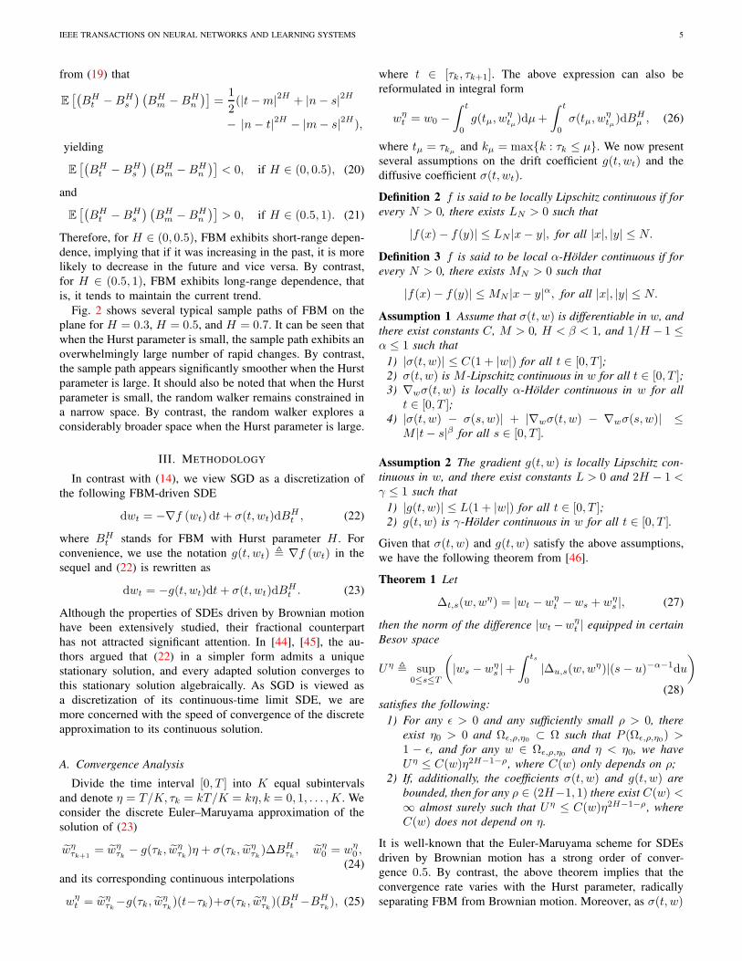
Fig. 3: Potential function with two local minima wa and wc
separated by a local maximum wb.
and g(t, w) are bounded in DNNs, as discussed previously,
the conclusion Uη ≤ C(w)η2H−1−ρ holds uniformly. This
indicates that the error between the discretization and the true
solution gained from SGD recursion is upper bounded and
scales as O(η2H−1−ρ). Thus, it is straightforward to conclude
that when the Hurst parameter is large, the corresponding SGD
recursion has a fast convergence rate.
B. First Passage Time Analysis
In this section, we present our main contribution associated
with the first passage time problem for FBM-driven SDEs.
The first passage time is the time t at which a stochastic
process passes over a barrier for the first time or escapes from
an interval by reaching the absorbing boundaries. Suppose
that wt is currently trapped in a suboptimal minimum wa,
as shown in Fig. 3, before sliding to another minimum wc,
we are interested in the time required to climb up to wb
from the bottom, as in metastability theory [47]. This is a
key problem in stochastic processes. However, except for
Brownian motion and several particular random processes,
there are few analytical results regrading to the Gaussian
processes.
Assumption 3 Assume that the stationary distribution of the
SGD recursion is constrained to a local region where the loss
function is well approximated by a quadratic function
f(w) =1
2(w − w0)A(w − w0)
T . (29)
Without loss of generality, we further assume that the min-
imum is attained at w0 = 0, and the Hessian matrix A is
semi-positive definite. This assumption has been empirically
justified in [48]. Thus, (23) reduces to
dwt = −Awtdt+ σ(t, wt)dBHt , (30)
the solution to which is known as a fractional Ornstein-
Uhlenbeck (OU) process [49]. For simplicity, we only consider
the one-dimensional situation
dwt = −awtdt+ σdBHt , (31)
where a is the corresponding diagonal entry of A and σ is a
constant owing to the stationarity in the latter training stages.
Resorting to the technique for deriving the ordinary Fokker-
Planck equation for Brownian motion [50], [51], we can obtain
the state probability density of neural network weight w at
time t.
Lemma 1 Let p(w, t) be the probability density function for
the neural network weight w at time t. Given that w follows
(31) with initial condition p(w, 0) = δ(w−w0), we explicitly
have
p(w, t) =1
2√πZt
exp
[− (w − e−atw0)
2
4Zt
], (32)
where
Zt =a−2H
2σ2H(2H − 1)Γ(2H − 1)
− H(2H − 1)t2H−1σ2
2aE2H−2(at)
− Ht2H−1σ2
2ae−2atM(2H − 1, 2H, at).
Here, Ep(t) is an integral exponential function
Ep(t) =
∫ ∞
1
x−pe−tx dx,
and M(a, b, t) is Kummer’s confluent hypergeometric function
M(a, b, t) =Γ(b)
Γ(a)Γ(b− a)
∫ 1
0
etxxa−1(1− x)b−a−1 dx.
To avoid clutter, we only give the proof sketch as follows and
defer the complete proof to Appendix A.
Sketch of Proof: Assume that at time t = 0, the neural
network weight w is located at w(0) = w0. And denote by
Yt the FGN corresponding to BHt . Integrating over (31), we
obtain
w(t;w0) = e−atw0 +
∫ t
0
e−a(t−τ)Yτ dτ. (33)
Moreover, the probability density function of w at time t is
given by the Dirac delta function
p(w, t;w0) = δ (w − w (t;w0)) . (34)
Now that the distribution of w0 is unknown, the state proba-
bility density of w at any time t is given by
p(w, t) =
∫p(w0, 0) 〈δ (w − w (t;w0))〉dw0, (35)
where 〈·〉 denotes an average over Yt. Recall that
δ(w) =1
2π
∫eiwxdx, (36)
and combine it with (35), we obtain the analytic expression
of p(x, t), which is the Fourier transform of p(w, t). Then,
according to
p(w, t) =1
2π
∫p(x, t)eiwxdx, (37)
we conclude the proof.
IEEE TRANSACTIONS ON NEURAL NETWORKS AND LEARNING SYSTEMS 7
Based on the analytical expression of p(w, t), the first
passage time density is obtained immediately.
Theorem 2 If t > 0 is sufficiently large, the probability
density function of the first passage time is approximately
given by
p(t) ≈ O(a3H t2H−2e−at
σ). (38)
The proof sketch is presented as follows and the complete
proof is shown in Appendix B.
Sketch of Proof: When t is sufficiently large, we will first
obtain an estimation of Z(t) by using the limiting approxima-
tion of E2H−2(at) and M(2H−1, 2H, at). Following a Taylor
expansion of exp
[− (w−e−atw0)
2
4Zt
], we are able to acquire an
estimation of p(w, t). Denote the survival probability by
s(t) =
∫p(w, t)dw, (39)
then, it is direct to obtain the first passage density
p(t) = −ds(t)
dt≈ O(
a3Ht2H−2e−at
σ). (40)
Remark 1 It should be noted that in previous works [52],
[53] motion correlations at different moments were neglected,
and a pseudo-Markovian scheme was utilized to approximate
the state probability density and obtain a similar result p(t) ≈O(t2H−2). However, for the case H > 1/2, the integral
for computing the mean passage time diverges. In numerical
simulations, this can be circumvented by using Feynman’s
path integral, as suggested in [54]. By contrast, the proposed
approximation provides a remedy and includes the dependence
on local curvature a and noise intensity σ.
Remark 2 Since the constant a indicates the curvature at the
local minimum; thus, by integrating (38) over time t, it is easy
to verify that: (1) it requires more time to exit for large a and
H; (2) it requires less time to exit for large σ. This observation
is empirically confirmed as well, see Fig. 8. This implies that
at early training stages, on one hand, larger noise helps SGD
effectively escape from sharp minima, while on the other hand,
at final stages, larger H enforces SGD to stay longer in flat, or
so-called wide, minima. This serves as an evident explanation
that SGD prefers wide minima that generalize well [26], [27].
IV. EXPERIMENTS
In this section, we conduct extensive experiments to support
our conjecture that SGN follows FBM instead of Brownian
motion or Lévy random process:
1) We first argue that SGN is neither a Gaussian nor a
Lévy stable distribution using existing statistical testing
methods;
2) Subsequently, we simulate a simple high-dimensional
SDE to verify that the convergence diversity is caused by
different fractional noises and that the Euclidean distance
from the initialization of network weights w correlates
well with the Hurst parameter;
3) In the third part, we study the mean escaping time of
the neural parameter w trapped in a harmonic potential
to demonstrate that a larger Hurst parameter yields a
lower escaping rate. Then, we approximately compute
the largest eigenvalue of the Hessian matrix for shallow
neural networks to verify that a large Hurst parameter
corresponds to flat minima;
4) Finally, we investigate the short-range memory effects
on a broad range of model architectures, datasets, and
training strategies.
Datasets. The datasets we use in the experiments are
MNIST, CIFAR10, and CIFAR100. We randomly split the
MNIST dataset into training and testing subsets of sizes 60K
and 10K, and the CIFAR10 and CIFAR100 datasets into
training and testing subsets of sizes 50K and 10K, respectively.
Several types of neural networks are utilized, including a fully
connected network (FCN) and several convolutional neural
networks (CNNs). The total model parameters scale from
thousands to millions, as is the case in most DNNs.
Implementation Details. We run every single model three
times with different random seeds, and the mean is plotted
throughout the experiments. To train the model parameters,
we select the vanilla SGD without additional techniques such
as momentum or weight decaying. Without any specification,
we use a batch size of 64 and a learning rate of 0.01. Similar to
large-scale studies [55], [56], we terminate the training process
once the cross-entropy loss decreases to a threshold of 0.01.
And we set the same batch size as in the training process to
estimate the SGN vectors. To reproduce the results, the code
is available at https://github.com/cltan023/shortRangeSGD.
Measurement Metric. We now introduce the estimation
method for the Hurst parameter. There are several such
techniques. However, as real-time series are finite in prac-
tice, and the local dynamics corresponding to a particular
temporal window can be over-estimated, no estimator can
be universally effective. Established approaches to estimating
the Hurst parameter can be classified into three categories.
They are applied either in the time domain, such as detrended
fluctuation and rescaled range analysis or in the frequency
domain, such as the wavelet and the periodogram method.
Alternatively, a radically different method called visibility
graph was proposed in [57], whereby the time series is mapped
onto a network using a visibility algorithm. An overview of
related work can be found in [58]. In this study, we use the
classical rescaled range (R/S) method [59] for simplicity and
efficiency.
Definition 4 Let Xiki=1 be a sequence of random variables
and the mean and standard deviation are given by
µ =1
k
k∑
i=1
Xi, Sk =
√√√√1
k
k∑
i=1
(Xi − µ)2. (41)
We define another two sequences Yiki=1 and Ztkt=1 re-
spectively by,
Yi = Xi − µ, i = 1, 2, · · · , k (42)
IEEE TRANSACTIONS ON NEURAL NETWORKS AND LEARNING SYSTEMS 8
♠❩ ❩ ♠❩ ❩
qP❳
❬❩ ❩ ❩❪
❩t Pt ❨
❬❨ ❨ ❨❪
❨ ❳
P ❳
❬❳❳ ❳❪
P
♦ ♦
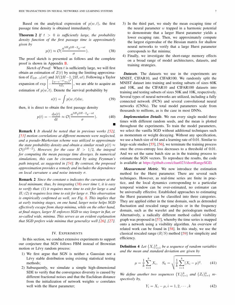
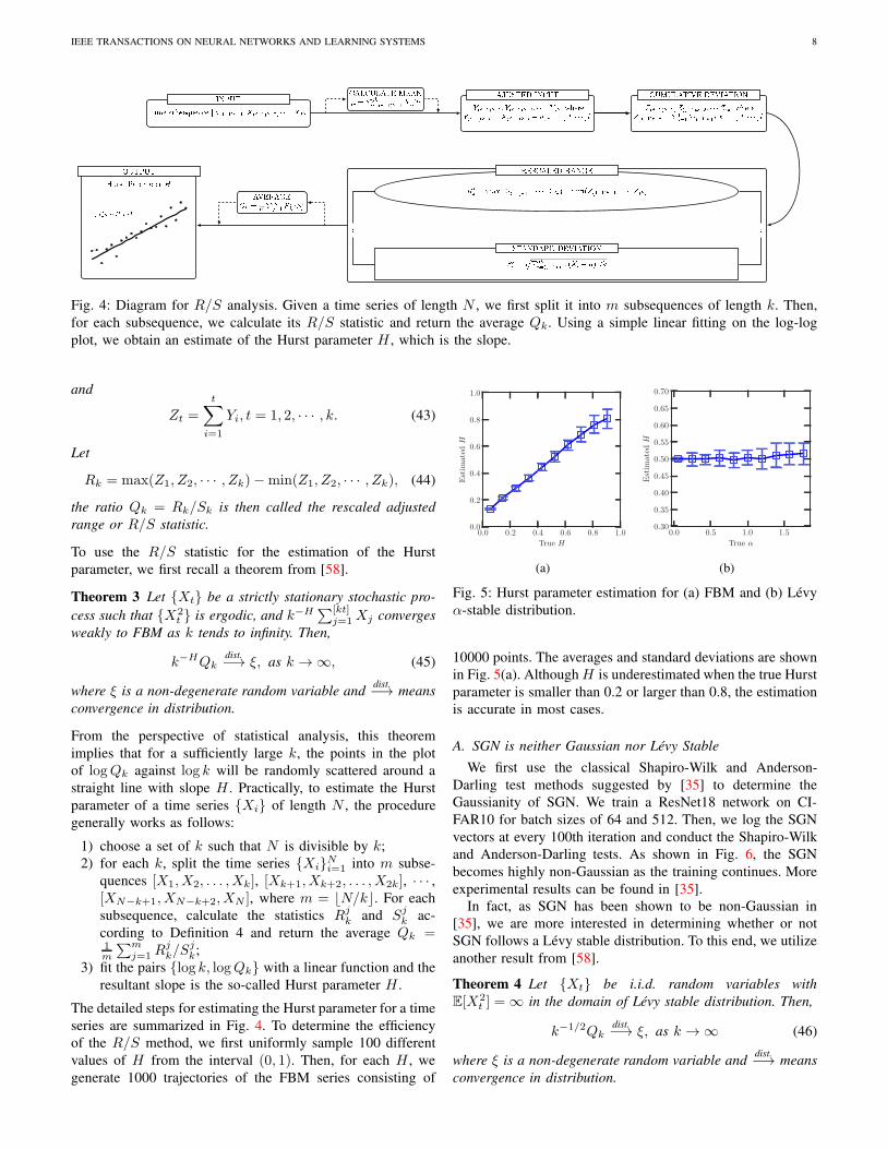
Fig. 4: Diagram for R/S analysis. Given a time series of length N , we first split it into m subsequences of length k. Then,
for each subsequence, we calculate its R/S statistic and return the average Qk. Using a simple linear fitting on the log-log
plot, we obtain an estimate of the Hurst parameter H , which is the slope.
and
Zt =t∑
i=1
Yi, t = 1, 2, · · · , k. (43)
Let
Rk = max(Z1, Z2, · · · , Zk)−min(Z1, Z2, · · · , Zk), (44)
the ratio Qk = Rk/Sk is then called the rescaled adjusted
range or R/S statistic.
To use the R/S statistic for the estimation of the Hurst
parameter, we first recall a theorem from [58].
Theorem 3 Let Xt be a strictly stationary stochastic pro-
cess such that X2t is ergodic, and k−H
∑[kt]j=1 Xj converges
weakly to FBM as k tends to infinity. Then,
k−HQkdist.−→ ξ, as k → ∞, (45)
where ξ is a non-degenerate random variable anddist.−→ means
convergence in distribution.
From the perspective of statistical analysis, this theorem
implies that for a sufficiently large k, the points in the plot
of logQk against log k will be randomly scattered around a
straight line with slope H . Practically, to estimate the Hurst
parameter of a time series Xi of length N , the procedure
generally works as follows:
1) choose a set of k such that N is divisible by k;
2) for each k, split the time series XiNi=1 into m subse-
quences [X1, X2, . . . , Xk], [Xk+1, Xk+2, . . . , X2k], · · · ,[XN−k+1, XN−k+2, XN ], where m = ⌊N/k⌋. For each
subsequence, calculate the statistics Rjk and Sj
k ac-
cording to Definition 4 and return the average Qk =1m
∑mj=1 R
jk/S
jk;
3) fit the pairs log k, logQk with a linear function and the
resultant slope is the so-called Hurst parameter H .
The detailed steps for estimating the Hurst parameter for a time
series are summarized in Fig. 4. To determine the efficiency
of the R/S method, we first uniformly sample 100 different
values of H from the interval (0, 1). Then, for each H , we
generate 1000 trajectories of the FBM series consisting of
0.0 0.2 0.4 0.6 0.8 1.0
True H
0.0
0.2
0.4
0.6
0.8
1.0
Estim
atedH
(a)
0.0 0.5 1.0 1.5
True α
0.30
0.35
0.40
0.45
0.50
0.55
0.60
0.65
0.70
Estim
atedH
(b)
Fig. 5: Hurst parameter estimation for (a) FBM and (b) Lévy
α-stable distribution.
10000 points. The averages and standard deviations are shown
in Fig. 5(a). Although H is underestimated when the true Hurst
parameter is smaller than 0.2 or larger than 0.8, the estimation
is accurate in most cases.
A. SGN is neither Gaussian nor Lévy Stable
We first use the classical Shapiro-Wilk and Anderson-
Darling test methods suggested by [35] to determine the
Gaussianity of SGN. We train a ResNet18 network on CI-
FAR10 for batch sizes of 64 and 512. Then, we log the SGN
vectors at every 100th iteration and conduct the Shapiro-Wilk
and Anderson-Darling tests. As shown in Fig. 6, the SGN
becomes highly non-Gaussian as the training continues. More
experimental results can be found in [35].
In fact, as SGN has been shown to be non-Gaussian in
[35], we are more interested in determining whether or not
SGN follows a Lévy stable distribution. To this end, we utilize
another result from [58].
Theorem 4 Let Xt be i.i.d. random variables with
E[X2t ] = ∞ in the domain of Lévy stable distribution. Then,
k−1/2Qkdist.−→ ξ, as k → ∞ (46)
where ξ is a non-degenerate random variable anddist.−→ means
convergence in distribution.

IEEE TRANSACTIONS ON NEURAL NETWORKS AND LEARNING SYSTEMS 9
0 20000 40000
Iterations
0.0
0.1
0.2
0.3
0.4
0.5
AveragepValue
Gaussian
BS = 64
BS = 512
(a)
0 20000 40000
Iterations
0.0
0.2
0.4
0.6
0.8
1.0
AcceptedFractionforGaussian
Gaussian
BS = 64
BS = 512
(b)
Fig. 6: (a) Shapiro-Wilk and (b) Anderson-Darling Gaussianity
test result for ResNet18 on CIFAR10. A smaller value implies
that the SGN is less likely to be Gaussian.
This theorem implies that if the SGN follows a Lévy stable
distribution, then estimations of the Hurst parameter in the
log-log plot are scattered around a straight line with a slope
of 0.5. Therefore, the reasoning line that SGN does not follow
a Lévy stable distribution becomes clear:
1) verify that if samples are generated from Lévy stable
distributions, then the estimated Hurst parameter is 0.5;
2) estimate the Hurst parameter of SGN, and if the estimated
Hurst parameter is far different from 0.5, then SGN does
not follow the Lévy stable distribution.
To validate 1), we first uniformly sample 100 different values
of α from the interval (0, 2). Then, for each α, we generate
1000 sequences of Lévy stable series with 10000 points.
Fig. 5(b) shows the averages and standard deviations. It can
be seen that the estimated Hurst parameter is not sensitive
to α and remains unchanged around the horizontal line of
H = 0.5. This implies that noise generated from a Lévy stable
distribution exhibits no sign of short-range memory effects. By
contrast, the Hurst estimation of the SGN from, for instance,
Figs. 10 and 11, is far away from 0.5 and varies according to
different hyperparameters. Therefore, it is reasonable to claim
that SGN does not follow a Lévy stable distribution.
B. Larger Hurst Parameter Indicates Faster Convergence
The convergence rate is of great interest in the study of
SDEs. Theorem 1 implies that the convergence rate of FBM-
driven SDEs is positively correlated with the Hurst parameter.
Herein, we experimentally confirm this theoretical observation
and provide further evidence that the SGN has short-range
memory.
It is well-recognized that large noise intensity in small
batch size encourages the neural weights w to go further
from the initialization [11], [60]. In this section, we provide
an alternative explanation and argue that it may result from
different Hurst parameters. We first train several ResNet18
models on CIFAR10 with different batch sizes and estimate
the corresponding Hurst parameters. It should be highlighted
that at each step of training, the noise intensity of all models
is tuned to the same magnitude, to cancel the effect of noise
intensity. As shown in Fig. 7 (a), the Euclidean distance of
0 25 50 75 100
Epochs
5
10
15
20
25
||w
k−w
0||
H = 0.38
H = 0.30
H = 0.27
BS = 64
BS = 256
BS = 512
(a)
0 5 10 15
Time
0
1
2
3
4
5
||w
t−w
0||
H = 0.38
H = 0.30
H = 0.27
(b)
Fig. 7: (a) Euclidean distance of neural network weights wfrom initialization for different batch sizes, and the corre-
sponding estimations of Hurst parameter. (b) Euclidean dis-
tance of the simulation of SDE from the origin driven by the
same Hurst parameters.
neural network weight w from the initialization still decreases
with the batch size.
Next, we apply the estimated Hurst parameters to the
following SDE
dwt = −2wtdt+ σdBHt , (47)
where wt ∈ Rd, and σ is a constant. Without loss of generality,
we assume that d = 100000 and σ = 0.01. With the initial
condition that w = 0, we are interested in the Euclidean
distance from the origin for different Hurst parameters as time
evolves. As shown in Fig. 7 (b), when the Hurst parameter is
larger, the solution converges at a faster rate and drifts further
away from the initialization. This is in line with Theorem 1;
therefore, except for the noise intensity, the Hurst parameter
is another major source of convergence diversity for different
batch sizes.
C. Larger Hurst Parameter Indicates Wider Minima
In this section, we study the escaping behavior from local
minima. For simplicity, we only consider one-dimensional
situation in which the neural network weight w is trapped in
a local minimum at w = 0. We assume that the loss function
around this point is convex and can be written as
f(w) =a
2w2. (48)
Thus, the dynamics in the vicinity of the local minimum can
be described as
dwt = −awtdt+ σdBHt . (49)
Without loss of generality, given an absorbing boundary w =±1, we are concerned with the mean time so that w can reach
this boundary. For this purpose, we select a time step η = 0.01,
and simulate 50 times for different Hurst parameters H =0.3, H = 0.5, and H = 0.7. To study the influence of local
curvature and noise intensity, we select a and the reciprocal of
σ2 both from the range 0.5, 1.0, 1.5, 2.0, 2.5. For each run,
we first generate a sequence of 105 FGN series as the noise
input. As can be seen from Fig. 8, the time for w to escape

IEEE TRANSACTIONS ON NEURAL NETWORKS AND LEARNING SYSTEMS 10
0.5 1.0 1.5 2.0 2.5
1/σ2
0
5
10
15
20
EscapingTim
e
H = 0.3
H = 0.5
H = 0.7
0.5 1.0 1.5 2.0 2.5
a
0
500
1000
1500
2000
EscapingTim
e
H = 0.3
H = 0.5
H = 0.7
H = 0.5
H = 0.5
Fig. 8: Influence of σ (upper panel) and a (lower panel) on the
mean escaping time of FBM-driven SDE at H = 0.3, H = 0.5and H = 0.7. For a = 2.5 and H = 0.7, it is noteworthy that
w fails to reach the absorbing boundary when the pre-specified
time expires. Thus, all points are truncated to concentrate on a
single value.The inset shows all the escaping times at H = 0.5in detail, and the line connects the means.
from the harmonic potential grows with the Hurst parameter.
Furthermore, it is heavily affected by the local curvature and
the noise intensity. It shows that it is difficult to escape from
a sharp bowl with a low noise intensity.
We now empirically confirm the assertion that larger Hurst
parameter leads to wider minima. To this end, we select a
single FCN and AlexNet as the base network. We train the
FCN network on MNIST, and AlexNet on CIFAR10. The
batch size is varied in 64, 128, · · · , 512. Similar to [25],
we compute the largest eigenvalue of the Hessian matrix at
the last iteration as a measure of flatness. Large eigenvalues
generally indicate sharp minima. Fig. 9 shows that the largest
eigenvalue increase with the batch size, whereas the Hurst
parameter changes in the opposite direction. This implies that
a small Hurst parameter results in large eigenvalues and tends
to end in sharp minima.
D. Impacts of Hyperparameters
Impacts of model capacity. We first investigate the influence
of model capacity on the Hurst parameter. For simple FCN
networks, we vary the width (number of neurons in each layer)
and depth (number of hidden layers). By contrast, for complex
CNN networks, we alter the scale (number of feature maps) in
each convolution layer. For FCN networks, we select the width
from 64, 128, · · · , 512 and the depth from 3, 4, · · · , 7,
and train 40 models in total on the MNIST dataset in each run.
As can be seen from Fig. 10, the Hurst parameter is sensitive
to the model architecture and decreases with the width and
64 128 192 256 320 384 448 512
Batch Size
0.250
0.275
0.300
0.325
0.350
0.375
0.400
H
H
Eigenvalue
14
16
18
20
22
24
26
LargestEigenvalue
(a)
64 128 192 256 320 384 448 512
Batch Size
0.26
0.28
0.30
0.32
0.34
0.36
0.38
0.40
H
H
Eigenvalue
20
40
60
80
100
LargestEigenvalue
(b)
Fig. 9: Estimation of the Hurst parameter and largest eigen-
value for different batch sizes: (a) FCN on MNIST; (b)
AlexNet on CIFAR10.
64 128 192 256 320 384 448 512
Width
0.400
0.405
0.410
0.415
0.420
0.425
H
Depth = 3
Depth = 4
(a)
3 4 5 6 7
Depth
0.38
0.39
0.40
0.41
0.42
H
Width = 256
Width = 512
(b)
Fig. 10: Estimation of the Hurst parameter for different widths
and depths for FCN networks on MNIST.
depth of the FCN. As to CNN networks, we select AlexNet
as the base model and range the filters in each layer from
64, 128, · · · , 512. Fig. 11 shows that the Hurst parameter is
highly sensitive to network scale, and monotonically increases
with model capacity on CIFAR10 and CIFAR100.
Impacts of batch size and learning rate. It is well-known
that a large batch size generally leads to sharp minima and thus
poor generalization. Herein, we examine the effects of batch
size on the Hurst parameter. According to the discussion in the
previous section, it is reasonable to conclude that the Hurst
parameter decreases with batch size. To further verify this
observation, we monitor the behavior of the Hurst parameters
for ResNet18 and VGG16_BN on CIFAR10 and CIFAR100.
The law that the Hurst parameter decreases with the batch size
is preserved, as shown in Figs. 12 and 13.
We also investigate the influence of the learning rate on the
Hurst parameter for ResNet18 and VGG16_BN. The learning
rate is selected from 0.0001, 0.0005, 0.001, 0.005, 0.01. As
can be seen from Fig. 14, the Hurst parameter increases with
the learning rate; this is aligned with the empirical observation
that a large learning rate leads to better generalization [17].
E. Impacts of LSTM and Attention Mechanism
Unlike traditional feedforward neural networks, LSTM [36]
has feedback connections, and excels at handling with natural
language processing tasks. More recently, another class of
models, Transformer [61], which is based on attention mecha-
nism, is proposed and is superior to LSTM in a wide spectrum

IEEE TRANSACTIONS ON NEURAL NETWORKS AND LEARNING SYSTEMS 11
64 128 192 256 320 384 448 512
Scale
0.37
0.38
0.39
0.40
0.41
0.42
H
H
Test Accuracy
0.75
0.76
0.77
0.78
0.79
0.80
TestAccuracy
(a)
64 128 192 256 320 384 448 512
Scale
0.31
0.32
0.33
0.34
0.35
0.36
0.37
H
H
Test Accuracy
0.36
0.38
0.40
0.42
0.44
0.46
0.48
TestAccuracy
(b)
Fig. 11: Estimation of the Hurst parameter and testing accuracy
across varying scales for AlexNet on (a) CIFAR10 and (b)
CIFAR100.
32 64 128 256 512 1024 2048
Batch Size
0.15
0.20
0.25
0.30
0.35
H
H
Test Accuracy
0.50
0.55
0.60
0.65
0.70
0.75
TestAccuracy
(a)
32 64 128 256 512 1024 2048
Batch Size
0.25
0.30
0.35
0.40
0.45
H
H
Test Accuracy
0.50
0.55
0.60
0.65
0.70
0.75
0.80
TestAccuracy
(b)
Fig. 12: Estimation of the Hurst parameter and test ac-
curacy across varying batch sizes for (a) ResNet18 and
(b)VGG16_BN on CIFAR10.
32 64 128 256 512 1024 2048
Batch Size
0.175
0.200
0.225
0.250
0.275
0.300
0.325
0.350
H
H
Test Accuracy
0.25
0.30
0.35
0.40
TestAccuracy
(a)
32 64 128 256 512 1024 2048
Batch Size
0.20
0.25
0.30
0.35
0.40
0.45
H
H
Test Accuracy
0.20
0.25
0.30
0.35
0.40
0.45
0.50
TestAccuracy
(b)
Fig. 13: Estimation of the Hurst parameter and test ac-
curacy across varying batch sizes for (a) ResNet18 and
(b)VGG16_BN on CIFAR100.
of applications. In this section, we investigate whether or not
the SGN still follows FBM in these two ad hoc network archi-
tectures for capturing long- and short-range inter-dependence.
We apply the LSTM on two sequential datasets, Disaster-
Tweets1 and FakeNews2, for the task of binary classification.
As to the Transformer model, we use the ViT [37], which
is particularly designed to extend the Transformer model to
image classification tasks.
We still look into how the Hurst parameter changes with
the batch size and learning rate. Due to limited GPU memory
(single NVIDIA RTX2080TI), for the ViT model we conduct
1https://www.kaggle.com/c/nlp-getting-started/data2https://www.kaggle.com/nopdev/real-and-fake-news-dataset
0.0001 0.0005 0.001 0.005 0.01
Learning Rate
0.31
0.32
0.33
0.34
H
H
Test Accuracy
0.63
0.64
0.65
0.66
0.67
0.68
0.69
0.70
TestAccuracy
(a)
0.0001 0.0005 0.001 0.005 0.01
Learning Rate
0.325
0.350
0.375
0.400
0.425
0.450
H
H
Test Accuracy
0.60
0.65
0.70
0.75
TestAccuracy
(b)
Fig. 14: Estimation of the Hurst parameter and test ac-
curacy across varying learning rates for (a) ResNet18 and
(b)VGG16_BN on CIFAR10.
0.0001 0.0005 0.001 0.005 0.01
Learning Rate
0.28
0.30
0.32
0.34
0.36
H
H
Test Accuracy
0.34
0.35
0.36
0.37
0.38
0.39
TestAccuracy
(a)
0.0001 0.0005 0.001 0.005 0.01
Learning Rate
0.300
0.325
0.350
0.375
0.400
0.425
0.450
H
H
Test Accuracy
0.300
0.325
0.350
0.375
0.400
0.425
0.450
TestAccuracy
(b)
Fig. 15: Estimation of the Hurst parameter and test ac-
curacy across varying learning rates for (a) ResNet18 and
(b)VGG16_BN on CIFAR100.
8 16 32 64 128 256
Batch Size
0.10
0.12
0.14
0.16
0.18
0.20
H
LR = 0.001
LR = 0.01
(a)
8 16 32 64 128 256
Batch Size
0.12
0.14
0.16
0.18
0.20
0.22
H
LR = 0.001
LR = 0.01
(b)
Fig. 16: Estimation of the Hurst parameter of LSTM on (a)
FakeNews and (b) DisasterTweets.
experiments with very small batches 8, 16, · · · , 80 and
mixed-precision training is also employed. As can be seen
from Figs. 16 and 17, the Hurst parameter is far away from
0.5, which suggests that SGN in LSTM and ViT is highly
non-Gaussian and follows FBM as well.
F. Impacts of Momentum and Weight Decaying
Though our theoretical analysis is based on vanilla SGD,
in this section we investigate the impacts of momentum and
weight decaying as both of them are indispensable ingre-
dients to achieve better results. To recover the influence of
different training strategies, we train ResNet18 on CIFAR10
with batches from 32, 64, · · · , 256 and learning rates from
IEEE TRANSACTIONS ON NEURAL NETWORKS AND LEARNING SYSTEMS 12
8 16 32 48 64 80
Batch Size
0.24
0.26
0.28
0.30
0.32
H
LR = 0.001
LR = 0.01
(a)
8 16 32 48 64 80
Batch Size
0.24
0.26
0.28
0.30
H
LR = 0.001
LR = 0.01
(b)
Fig. 17: Estimation of the Hurst parameter of ViT on (a)
CIFAR10 and (b) CIFAR100.
32 64 96 128 160 192 224 256
Batch Size
0.26
0.28
0.30
0.32
0.34
H
LR = 0.001
LR = 0.01
(a)
32 64 96 128 160 192 224 256
Batch Size
0.26
0.28
0.30
0.32
0.34
0.36
0.38
H
LR = 0.001
LR = 0.01
(b)
32 64 96 128 160 192 224 256
Batch Size
0.26
0.28
0.30
0.32
0.34
H
LR = 0.001
LR = 0.01
(c)
32 64 96 128 160 192 224 256
Batch Size
0.26
0.28
0.30
0.32
0.34
0.36
H
LR = 0.001
LR = 0.01
(d)
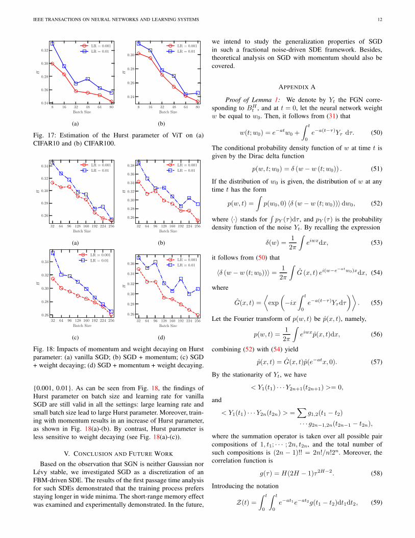
Fig. 18: Impacts of momentum and weight decaying on Hurst
parameter: (a) vanilla SGD; (b) SGD + momentum; (c) SGD
+ weight decaying; (d) SGD + momentum + weight decaying.
0.001, 0.01. As can be seen from Fig. 18, the findings of
Hurst parameter on batch size and learning rate for vanilla
SGD are still valid in all the settings: large learning rate and
small batch size lead to large Hurst parameter. Moreover, train-
ing with momentum results in an increase of Hurst parameter,
as shown in Fig. 18(a)-(b). By contrast, Hurst parameter is
less sensitive to weight decaying (see Fig. 18(a)-(c)).
V. CONCLUSION AND FUTURE WORK
Based on the observation that SGN is neither Gaussian nor
Lévy stable, we investigated SGD as a discretization of an
FBM-driven SDE. The results of the first passage time analysis
for such SDEs demonstrated that the training process prefers
staying longer in wide minima. The short-range memory effect
was examined and experimentally demonstrated. In the future,
we intend to study the generalization properties of SGD
in such a fractional noise-driven SDE framework. Besides,
theoretical analysis on SGD with momentum should also be
covered.
APPENDIX A
Proof of Lemma 1: We denote by Yt the FGN corre-
sponding to BHt , and at t = 0, let the neural network weight
w be equal to w0. Then, it follows from (31) that
w(t;w0) = e−atw0 +
∫ t
0
e−a(t−τ)Yτ dτ. (50)
The conditional probability density function of w at time t is
given by the Dirac delta function
p(w, t;w0) = δ (w − w (t;w0)) . (51)
If the distribution of w0 is given, the distribution of w at any
time t has the form
p(w, t) =
∫p(w0, 0) 〈δ (w − w (t;w0))〉dw0, (52)
where 〈·〉 stands for∫pY (τ)dτ , and pY (τ) is the probability
density function of the noise Yt. By recalling the expression
δ(w) =1
2π
∫eiwxdx, (53)
it follows from (50) that
〈δ (w − w (t;w0))〉 =1
2π
∫G (x, t) ei(w−e−atw0)xdx, (54)
where
G(x, t) =
⟨exp
(−ix
∫ t
0
e−a(t−τ)Yτdτ
)⟩. (55)
Let the Fourier transform of p(w, t) be p(x, t), namely,
p(w, t) =1
2π
∫eiwxp(x, t)dx, (56)
combining (52) with (54) yield
p(x, t) = G(x, t)p(e−atx, 0). (57)
By the stationarity of Yt, we have
< Y1(t1) · · ·Y2n+1(t2n+1) >= 0,
and
< Y1(t1) · · ·Y2n(t2n) > =∑
g1,2(t1 − t2)
· · · g2n−1,2n(t2n−1 − t2n),
where the summation operator is taken over all possible pair
compositions of 1, t1; · · · ; 2n, t2n, and the total number of
such compositions is (2n − 1)!! = 2n!/n!2n. Moreover, the
correlation function is
g(τ) = H(2H − 1)τ2H−2. (58)
Introducing the notation
Z(t) =
∫ t
0
∫ t
0
e−at1e−at2g(t1 − t2)dt1dt2, (59)

IEEE TRANSACTIONS ON NEURAL NETWORKS AND LEARNING SYSTEMS 13
and expanding G(x, t) in a Taylor series, we obtain
G(x, t) =
∞∑
0
1
(2n)!
(2n)!
n!2n(−i)2nZn(t)x2n (60)
or equivalently
G(x, t) = e−Z(t)x2
. (61)
Since
p(x, 0) =
∫dwδ(w − w0)e
ixw = eiw0x (62)
and
p(e−atx, 0) = exp(−iw0e−atx), (63)
combining with (61) yields
p(w, t) =1
2π
∫p(x, t)eiwxdx
=1
2π
∫G(x, t)p(e−atx, 0)eiwxdx
=1
2π
∫e−Z(t)x2
exp(−iw0e−atx)eiwxdx
=1
2√πZ(t)
exp
[− (w − e−atw0)
2
4Zt
].
(64)
We now proceed to compute the expression Z(t). Calculating
the expression Z(t) can be rather involved; thus, we introduce
a change of variables to obtain a more tractable form
Z(t) =
∫ t
0
g(τ)
∫ t−τ
0
e−a(T+τ)e−aTdτdT
= σ2H(2H − 1)
∫ t
0
τ2H−2e−aτ (− 1
2a)e−2aT |t−τ
0 dτ
=1
2aσ2H(2H − 1)
∫ t
0
τ2H−2(e−aτ − eaτe−2at
)dτ.
(65)
We note that the first term inside the brackets is∫ t
0
τ2H−2e−aτdτ =
∫ t
0
(τ
t)2H−2t2H−2e−at τ
t dτ
= t2H−1
∫ 1
0
τ2H−2e−atτdτ (66)
= t2H−1(
∫ ∞
0
τ2H−2e−atτdτ
−∫ ∞
1
τ2H−2e−atτdτ)
= a1−2HΓ(2H − 1)− t2H−1E2−2H(at),
whereas the second term is∫ t
0
τ2H−2eaτe−2atdτ = e−2at
∫ t
0
τ2H−2eaτdτ
= e−2att2H−1
∫ 1
0
τ2H−2eatτdτ
=t2H−1
2H − 1e−2atM(2H − 1, 2H, at).
(67)
Combining (64)–(67) concludes the proof.
APPENDIX B
Proof of Theorem 2: On one hand, when t is sufficiently
large, ∫ t
0
τ2H−2e−aτdτ ≈ a1−2HΓ(2H − 1). (68)
On the other hand, since
M(2H−1, 2H, at) ≈ 2H − 1
ateat+Γ(2H)(−at)1−2H , (69)
we have∫ t
0
τ2H−2eaτe−2atdτ ≈ t2H−2
ae−at. (70)
Combining (70), (68) and (65), it is direct to conclude that
Z(t) ≈ H(2H − 1)
2a2HΓ(2H − 1)σ2 (71)
− σ2
2a2H(2H − 1)t2H−1 e
−at
at
=H(2H − 1)
2a2HΓ(2H − 1)σ2
(1− t2H−2e−at
Γ(2H − 1)a2−2H
).
Using the Taylor expansion of exponential function, we have
p(w, t) =1
2√πZt
exp
[− (w − e−atw0)
2
4Zt
](72)
≈ aH√2πΓ(2H − 1)H(2H − 1)σ2
×(1− a2H−2t2H−2e−at
2Γ(2H − 1)+ · · ·
)
×(1− (w − e−atw0)
2
4Zt+ · · ·
)(73)
≈ C1 + C2a3Ht2H−2e−at
σ(1 + C3w + C4w
2 + · · · ).
where C1, C2, C3, C4 are constants. Recall that the survival
probability s(t) is the probability that the random walker
remains in the domain up to time t, and it can be expressed
as
s(t) =
∫p(w, t)dw. (74)
Hence, the first passage time density is directly obtained from
p(t) = −ds(t)
dt≈ O(
a3H t2H−2e−at
σ). (75)
REFERENCES
[1] H. E. Hurst, “Long-term storage capacity of reservoirs,” Trans. Amer.
Soc. Civil Eng., vol. 116, pp. 770–799, 1951.
[2] R. Black, H. Hurst, and Y. Simaika, Long-term Storage: An Experimental
Study. Constable, 1965.
[3] N. Yuan, Z. Fu, and S. Liu, “Extracting climate memory using fractionalintegrated statistical model: A new perspective on climate prediction,”Sci. Rep., vol. 4, pp. 1–10, 2014.
[4] R. Cont, “Long range dependence in financial markets,” Fractals inEngineering, pp. 159–179, 2005.
[5] M. Grossglauser and J.-C. Bolot, “On the relevance of long-rangedependence in network traffic,” IEEE/ACM Trans. Networking, vol. 7,no. 5, pp. 629–640, 1999.
IEEE TRANSACTIONS ON NEURAL NETWORKS AND LEARNING SYSTEMS 14
[6] T. Karagiannis, M. Molle, and M. Faloutsos, “Long-range dependenceten years of internet traffic modeling,” IEEE Internet Comput., vol. 8,no. 5, pp. 57–64, 2004.
[7] J. Duchi, E. Hazan, and Y. Singer, “Adaptive subgradient methodsfor online learning and stochastic optimization,” J. Mach. Learn. Res,vol. 12, no. 61, pp. 2121–2159, 2011.
[8] D. P. Kingma and J. Ba, “Adam: A method for stochastic optimization,”in Proc. Int. Conf. Learn. Represent., 2015, pp. 1–15.
[9] N. S. Keskar, D. Mudigere, J. Nocedal, M. Smelyanskiy, and P. T. P.Tang, “On large-batch training for deep learning: Generalization gap andsharp minima,” in Proc. Int. Conf. Learn. Represent., 2017, pp. 1–16.
[10] C. Zhang, S. Bengio, M. Hardt, B. Recht, and O. Vinyals, “Understand-ing deep learning requires rethinking generalization,” in Proc. Int. Conf.Learn. Represent., 2017, pp. 1–15.
[11] E. Hoffer, I. Hubara, and D. Soudry, “Train longer, generalize better:Closing the generalization gap in large batch training of neural net-works,” in Proc. Adv. Neural Inf. Process. Syst., 2017, pp. 1731–1741.
[12] S. Jastrzebski, Z. Kenton, D. Arpit, N. Ballas, A. Fischer, Y. Bengio,and A. Storkey. (2017) Three factors influencing minima in SGD.[Online]. Available: https://arxiv.org/abs/1711.04623
[13] Z. Zhu, J. Wu, B. Yu, L. Wu, and J. Ma, “The anisotropic noise instochastic gradient descent: Its behavior of escaping from sharp minimaand regularization effects,” in Proc. Int. Conf. Mach. Learn., 2019, pp.7654–7663.
[14] L. Bottou, F. E. Curtis, and J. Nocedal, “Optimization methods for large-scale machine learning,” SIAM Rev., vol. 60, no. 2, pp. 223–311, 2018.
[15] S. L. Smith, P.-J. Kindermans, C. Ying, and Q. V. Le, “Don’t decaythe learning rate, increase the batch size,” in Proc. Int. Conf. Learn.
Represent., 2018, pp. 1–11.[16] Z. Yao, A. Gholami, Q. Lei, K. Keutzer, and M. W. Mahoney, “Hessian-
based analysis of large batch training and robustness to adversaries,” inProc. Adv. Neural Inf. Process. Syst., 2018, pp. 4949–4959.
[17] F. He, T. Liu, and D. Tao, “Control batch size and learning rate togeneralize well: Theoretical and empirical evidence,” in Proc. Adv.Neural Inf. Process. Syst., 2019, pp. 1143–1152.
[18] J. Wu, W. Hu, H. Xiong, J. Huan, V. Braverman, and Z. Zhu, “Onthe noisy gradient descent that generalizes as SGD,” in Proc. Int. Conf.
Mach. Learn., 2020, pp. 1–21.[19] S. Mandt, M. D. Hoffman, and D. M. Blei, “Stochastic gradient descent
as approximate Bayesian inference,” J. Mach. Learn. Res, vol. 18, no. 1,pp. 4873–4907, 2017.
[20] Q. Li, C. Tai, and E. Weinan, “Stochastic modified equations andadaptive stochastic gradient algorithms,” in Proc. Int. Conf. Mach.
Learn., 2017, pp. 2101–2110.[21] P. Chaudhari and S. Soatto, “Stochastic gradient descent performs
variational inference, converges to limit cycles for deep networks,” inProc. IEEE Inf. Teory Appl., 2018, pp. 1–10.
[22] W. Hu, C. J. Li, L. Li, and J.-G. Liu, “On the diffusion approximationof nonconvex stochastic gradient descent,” Ann. Math. Sci. Appl., vol. 4,no. 1, pp. 3–32, 2019.
[23] G. E. Hinton and D. Van Camp, “Keeping the neural networks simpleby minimizing the description length of the weights,” in Proc. Conf.Learn. Theory, 1993, pp. 5–13.
[24] S. Hochreiter and J. Schmidhuber, “Flat minima,” Neural Compt., vol. 9,no. 1, pp. 1–42, 1997.
[25] P. Chaudhari, A. Choromanska, S. Soatto, Y. LeCun, C. Baldassi,C. Borgs, J. Chayes, L. Sagun, and R. Zecchina, “Entropy-SGD: Biasinggradient descent into wide valleys,” in Proc. Int. Conf. Learn. Represent.,2019, pp. 1–19.
[26] U. Simsekli, L. Sagun, and M. Gurbuzbalaban, “A tail-index analysis ofstochastic gradient noise in deep neural networks,” in Proc. Int. Conf.
Mach. Learn., 2019, pp. 5827–5837.[27] T. H. Nguyen, U. Simsekli, M. Gurbuzbalaban, and G. Richard, “First
exit time analysis of stochastic gradient descent under heavy-tailedgradient noise,” in Proc. Adv. Neural Inf. Process. Syst., 2019, pp. 273–283.
[28] Y. Pawitan, In All Likelihood: Statistical Modelling and Inference Using
Likelihood. Oxford University Press, 2001.[29] R. Shwartz-Ziv and N. Tishby. (2017) Opening the black box
of deep neural networks via information. [Online]. Available:https://arxiv.org/abs/1703.00810
[30] L. Dinh, R. Pascanu, S. Bengio, and Y. Bengio, “Sharp minima cangeneralize for deep nets,” in Proc. Int. Conf. Mach. Learn., 2017, pp.1019–1028.
[31] Z. Xie, I. Sato, and M. Sugiyama, “A diffusion theory for deep learningdynamics: Stochastic gradient descent exponentially favors flat minima,”in Proc. Int. Conf. Learn. Represent., 2021, pp. 1–28.
[32] S. Ioffe and C. Szegedy, “Batch normalization: Accelerating deepnetwork training by reducing internal covariate shift,” in Proc. Int. Conf.Mach. Learn., 2015, pp. 448–456.
[33] K. He, X. Zhang, S. Ren, and J. Sun, “Delving deep into rectifiers:Surpassing human-level performance on Imagenet classification,” inProc. Int. Conf. Comput. Vis., 2015, pp. 1026–1034.
[34] X. Glorot and Y. Bengio, “Understanding the difficulty of training deepfeedforward neural networks,” in Proc. Int. Conf. Artif. Intell. Stat., 2010,pp. 249–256.
[35] A. Panigrahi, R. Somani, N. Goyal, and P. Netrapalli. (2019)Non-Gaussianity of stochastic gradient noise. [Online]. Available:https://arxiv.org/abs/1910.09626
[36] S. Hochreiter and J. Schmidhuber, “Long short-term memory,” Neural
Comput., vol. 9, no. 8, pp. 1735–1780, 1997.
[37] A. Dosovitskiy, L. Beyer, A. Kolesnikov, D. Weissenborn, X. Zhai,T. Unterthiner, M. Dehghani, M. Minderer, G. Heigold, S. Gelly et al.,“An image is worth 16x16 words: Transformers for image recognitionat scale,” in Proc. Int. Conf. Learn. Represent., 2021, pp. 1–22.
[38] A. N. Kolmogorov, “Curves in Hilbert space which are invariant withrespect to a one-parameter group of motions,” in Dokl. Akad. Nauk SSSR,vol. 26, no. 1, 1940, pp. 6–9.
[39] A. M. Yaglom, “Correlation theory of processes with random stationaryn th increments,” Matematicheskii Sbornik, vol. 79, no. 1, pp. 141–196,1955.
[40] B. B. Mandelbrot and J. W. Van Ness, “Fractional Brownian motions,fractional noises and applications,” SIAM Rev., vol. 10, no. 4, pp. 422–437, 1968.
[41] W. E. Leland, M. S. Taqqu, W. Willinger, and D. V. Wilson, “On theself-similar nature of ethernet traffic (extended version),” IEEE/ACM
Trans. Networking, vol. 2, no. 1, pp. 1–15, 1994.
[42] J. Y. Campbell, J. J. Champbell, J. W. Campbell, A. W. Lo, A. W. Lo, andA. C. MacKinlay, The Econometrics of Financial Markets. PrincetonUniversity Press, 1997.
[43] B. Mandelbrot, “How long is the coast of britain? Statistical self-similarity and fractional dimension,” Science, vol. 156, no. 3775, pp.636–638, 1967.
[44] M. Hairer, “Ergodicity of stochastic differential equations driven byfractional Brownian motion,” Ann. Probab., vol. 33, no. 2, pp. 703–758,2005.
[45] A. Rascanu et al., “Differential equations driven by fractional brownianmotion,” Collect. Math., vol. 53, no. 1, pp. 55–81, 2002.
[46] Y. Mishura and G. Shevchenko, “The rate of convergence for Eulerapproximations of solutions of stochastic differential equations drivenby fractional Brownian motion,” Stochastics, vol. 80, no. 5, pp. 489–511, 2008.
[47] P. Hanggi, “Escape from a metastable state,” J. Stat. Phys., vol. 42, no.1-2, pp. 105–148, 1986.
[48] H. Li, Z. Xu, G. Taylor, C. Studer, and T. Goldstein, “Visualizing theloss landscape of neural nets,” in Proc. Adv. Neural Inf. Process. Syst.,2018, pp. 6389–6399.
[49] P. Cheridito, H. Kawaguchi, M. Maejima et al., “Fractional Ornstein-Uhlenbeck processes,” Electron. J. Probab., vol. 8, pp. 1–14, 2003.
[50] A. I. Akhiezer and S. V. Peletminskii, Methods of Statistical Physics:
International Series in Natural Philosophy. Elsevier, 2013.
[51] O. Y. Sliusarenko. (2011) Generalized Fokker-Planck equation andits solution for linear non-Markovian Gaussian systems. [Online].Available: https://arxiv.org/abs/1107.0796
[52] O. Y. Sliusarenko, V. Y. Gonchar, A. V. Chechkin, I. M. Sokolov, andR. Metzler, “Kramers-like escape driven by fractional Gaussian noise,”Phys. Rev. E, vol. 81, no. 4, pp. 1–14, 2010.
[53] L. P. Sanders and T. Ambjörnsson, “First passage times for a tracerparticle in single file diffusion and fractional Brownian motion,” J.
Chem. Phys., vol. 136, no. 17, pp. 1–29, 2012.
[54] G. Jumarie, “Stochastic differential equations with fractional Brownianmotion input,” Int. J. Syst. Sci., vol. 24, no. 6, pp. 1–20, 1993.
[55] Y. Jiang, B. Neyshabur, H. Mobahi, D. Krishnan, and S. Bengio,“Fantastic generalization measures and where to find them,” in Proc.Int. Conf. Learn. Represent., 2020, pp. 1–33.
[56] G. K. Dziugaite, A. Drouin, B. Neal, N. Rajkumar, E. Caballero,L. Wang, I. Mitliagkas, and D. M. Roy, “In search of robust measuresof generalization,” in Proc. Adv. Neural Inf. Process. Syst., 2020, pp.1–27.
[57] L. Lacasa, B. Luque, J. Luque, and J. C. Nuno, “The visibility graph: Anew method for estimating the Hurst exponent of fractional Brownianmotion,” Europhys. Lett., vol. 86, no. 3, pp. 1–5, 2009.
[58] P. Embrechts, Selfsimilar Processes. Princeton University Press, 2009.
IEEE TRANSACTIONS ON NEURAL NETWORKS AND LEARNING SYSTEMS 15
[59] B. Qian and K. Rasheed, “Hurst exponent and financial market pre-dictability,” in Proc. IASTED Int. Conf., 2004, pp. 203–209.
[60] N. S. Keskar, D. Mudigere, J. Nocedal, M. Smelyanskiy, and P. T. P.Tang, “On large-batch training for deep learning: Generalization gap andsharp minima,” in Proc. Int. Conf. Learn. Represent., 2017, pp. 1–16.
[61] A. Vaswani, N. Shazeer, N. Parmar, J. Uszkoreit, L. Jones, A. N. Gomez,Ł. Kaiser, and I. Polosukhin, “Attention is all you need,” in Proc. Adv.
Neural Inf. Process. Syst., 2017, pp. 6000–6010.
Chengli Tan received the B.S. degree in informationand computing science and the M.S. degree in statis-tics from Xi’an Jiaotong University, Xi’an, China,in 2014 and 2017, where he is now pursuing thePh.D. degree. His current research interests includeadversarial learning, Bayesian nonparametrics, andstochastic optimization.
Jiangshe Zhang received the B.S., M.S., and Ph.D.degrees in computational mathematics from Xi’anJiaotong University, Xi’an, China, in 1984, 1987,and 1993, respectively. He is currently the Directorof the Institute of Machine Learning and StatisticalDecision Making, Xi’an Jiaotong University, wherehe is a Professor with the Department of Statistics.He is also the Vice-President of the Xi’an Interna-tional Academy for Mathematics and MathematicalTechnology, Xi’an, China. He has authored andco-authored one monograph and over 100 journal
papers. His research interests include statistical computing, deep learning,cognitive representation, and statistical decision-making.
Prof. Zhang received the National Natural Science Award of China (ThirdPlace) and the First Prize in Natural Science from the Ministry of Educationof China in 2007. He served as the President of the Shaanxi MathematicalSociety and the Executive Director of the China Mathematical Society.
Junmin Liu received a Ph.D. in applied mathemat-ics from Xi’an Jiaotong University, Xi’an, China in2013. He is currently an Associate Professor in theSchool of Mathematics and Statistics, Xi’an JiaotongUniversity, Xi’an, China. From 2014 to 2015, hewas a visiting scholar at the University of Maryland,College Park. His research interests are focused onmachine learning and computer vision.