Understanding Fundamental Property Equations through 3D Phase Diagrams Ríos-Casas,L.G.*, Alarcón-García,A., Chavela-Guerra,R.C., Márquez-Juárez,C.E. Gutiérrez-Vélez,J.X. Chemical and Food Engineering Department. Universidad de las Américas, Puebla. Ex – hacienda Santa Catarina Mártir. San Andrés Cholula, Puebla. C.P. 72820. México. E-mail: luisg.rios@udlap.mx ABSTRACT

This paper describes an effective visual approach to teach the fundamental and state equations for the thermodynamic properties of pure components. The methodology is based on obtaining, through the laws of Thermodynamics and the Maxwell relations, expressions for each property as a function of other two variables. From these equations and taking advantage of the excellent graphical capabilities of Matlab®, the reported data for water in the steam tables were used to generate the corresponding 3D phase diagrams. The equations analized and the visualizations produced are presented to demonstrate the great advantage of this method over a purely mathematical presentation. This material has been applied in the first Thermodynamics course at undergraduate level with excellent results. INTRODUCTION

The fundamental property equations and the Maxwell relations are essential concepts to understand the relationship between the thermodynamic properties and the state variables of a system. Unfortunately, the Chemical Engineering student finds difficult to grasp the meaning of these abstract concepts when presented only by mathematical expressions.

In the last decades, there have been important advances in generating figures to represent the behavior of themodynamic properties. Some examples of this are the work of Jolls (1990), Coy (1993) and Ríos et. al. (2003). Eventhough, it is difficult to find references presenting all the diagrams of practical importance. Moreover, nearly all the diagrams widely reported are 2D, when it is prefered to visualize functions of two variables as 3D surfaces.

The objective of this work is to generate a comprehensive collection of all the equations and diagrams of interest to the Chemical Engineering student, with the aim of increasing the understanding about this topic. METHODOLOGY

The Gibbs rule phase gives the minimum number of independent properties that completely define the state of a system. For a pure component in homogeneous phase, two properties must be fixed to determine all the extensive properties of the system; for vapor-liquid equilibrium, it requires to fix only one intensive property, either temperature or pressure.

The fundamental property relations are obtained from the sustitution of the first and second Law of Thermodynamics to define the thermodynamic equilibrium state of a closed system, thus the independent variables can not be chosen arbitrarily. On the other hand, by selecting the most convenient independent variables and introducing the Maxwell relations, the fundamental property equations are modified to relate the thermodynamic properties with measurable variables. Since the new functions resulting from this process are in terms of P, V and T, their plots have the great advantage of providing physical meaning to definitions that otherwise are completely intangible.

For this work, the thermodynamic properties data for water are plotted in 3D to represent the resulting equations for U (internal energy), H (enthalpy), S (entropy), G (Gibbs free energy) and A (Helmholtz free energy). Tha database was taken from Haar et. al. (1984) and introduced in Matlab® using the visualization tools. Different colors were used to distinguish the various regions: homogeneous liquid phase (blue), homogeneous gas phase (red), vapor-liquid region (cyan) and supercritical fluid (yellow). It is important to observe that mesh is constructed from values at constant temperature and pressure, in correspondece with the tabuleted data in the steam tables. The curves inside the vapor-liquid region stand for constant vapor fraction. RESULTS

For internal energy, the two independent variables resulting from applying the laws of Thermodynamics and the equilibrium state are S and V:

( ) ( ) ( ),i i

i i i i i i iV SdU S V T S dS P V dV= −

( ), , i i iU f S V phase, i pure=

This equation gives the first surface representing U as a function of S and V, as shown in Figure 1:

Figure 1. U=f(V,S) diagram for water.

It is possible to analize the efects of a change in volume at constant T:

i i idU TdS PdV= −

i i i

i i iT T T

U S VT PV V V

∂ ∂ ∂= − ∂ ∂ ∂

i i

i iT T T

U ST PV V

∂ ∂= − ∂ ∂

Now, T and V are conveniently chosen as variables to study the changes in the internal energy:

( ),iU f T V, phase, i pure=

( )( ) ( )

, i

i

i V i i Ti i i

i TV

U T U VdU T V dT dV

T V

∂ ∂ = + ∂ ∂

the first term is defined as the constant volume heat capacity:

( )( , phase )i

i

i

i VV V

V

U TC T , i pure

T

∂ = ∂

The study of a change in volume at constant T leads to analize the effect of volume in entropy at constant T, with the inconvenient of being a non-measurable or derived property:

( )i i iT

i i TT T

U V ST PV V

∂ ∂= − ∂ ∂

( ) ( ), , ii i V i i

i T T

SdU T V C T fase dT T P dVV

∂= + − ∂

This makes necessary to study the fundamental equation for A, obtained through its definition A = U – TS:

( ) ( ) ( ),i

i i i i iT VdA V T P V dV S T dT= − −

( ), , i iA f V T phase , i pure=

Figure 2 represents the relation among these properties:

Figure 2. A=f(V,T) diagram for water. Analyzing a differential change in A:

( ) ( ) ( ), i

i

i Vi i Ti i i

i T V

A TA VdA V T dV dT

V T

∂ ∂ = + ∂ ∂

( )i i T

i T

A VP

V ∂

= − ∂

( )

i

i

i Vi

V

A TS

T

∂ = − ∂

2

i

i

Vi

A PT V T∂ ∂ = − ∂ ∂ ∂

2

i i

i i T

A SV T V

∂ ∂= − ∂ ∂ ∂

it is possible to obtain the Maxwell relation:

i

i

V i T

SPT V

∂∂ = ∂ ∂

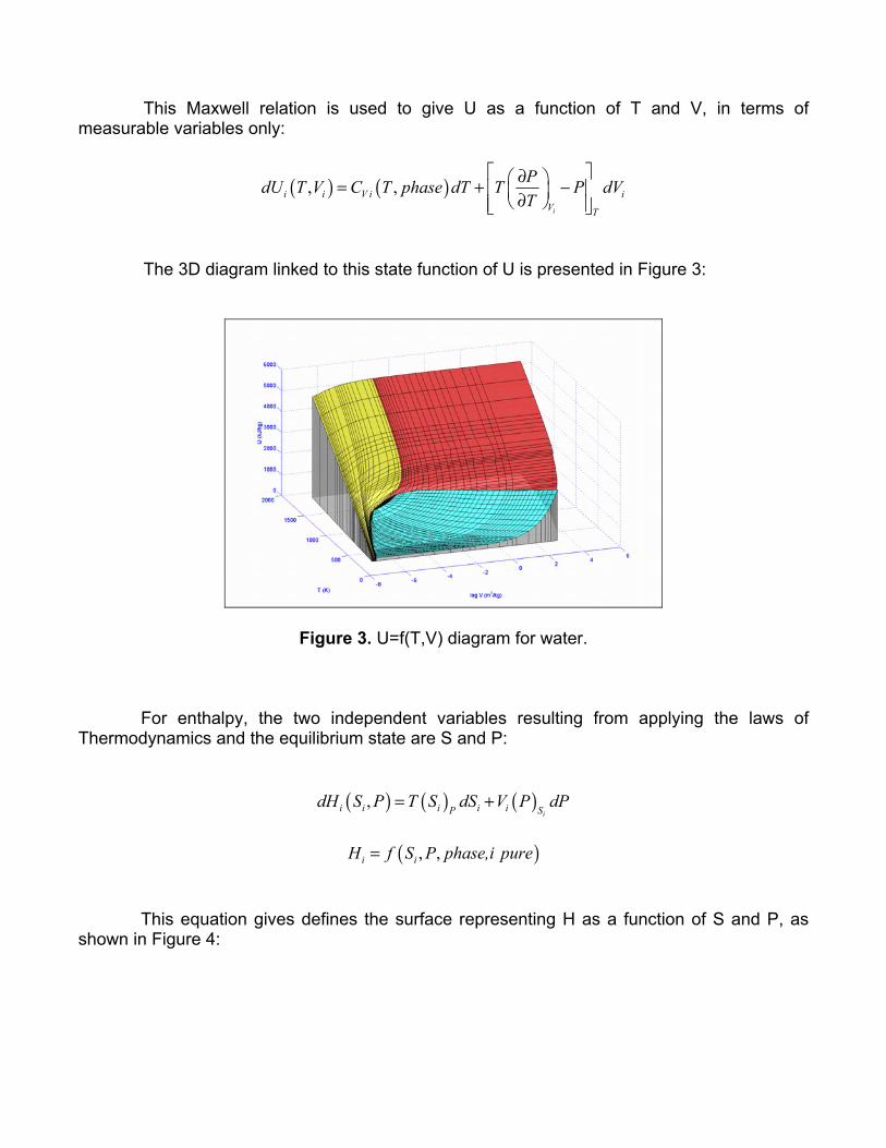
This Maxwell relation is used to give U as a function of T and V, in terms of measurable variables only:

( ) ( ), , i

i i V i iV T

PdU T V C T phase dT T P dVT

∂ = + − ∂

The 3D diagram linked to this state function of U is presented in Figure 3:

Figure 3. U=f(T,V) diagram for water.

For enthalpy, the two independent variables resulting from applying the laws of Thermodynamics and the equilibrium state are S and P:

( ) ( ) ( ),i

i i i i iP SdH S P T S dS V P dP= +

( ), ,i iH f S P phase,i pure=

This equation gives defines the surface representing H as a function of S and P, as shown in Figure 4:

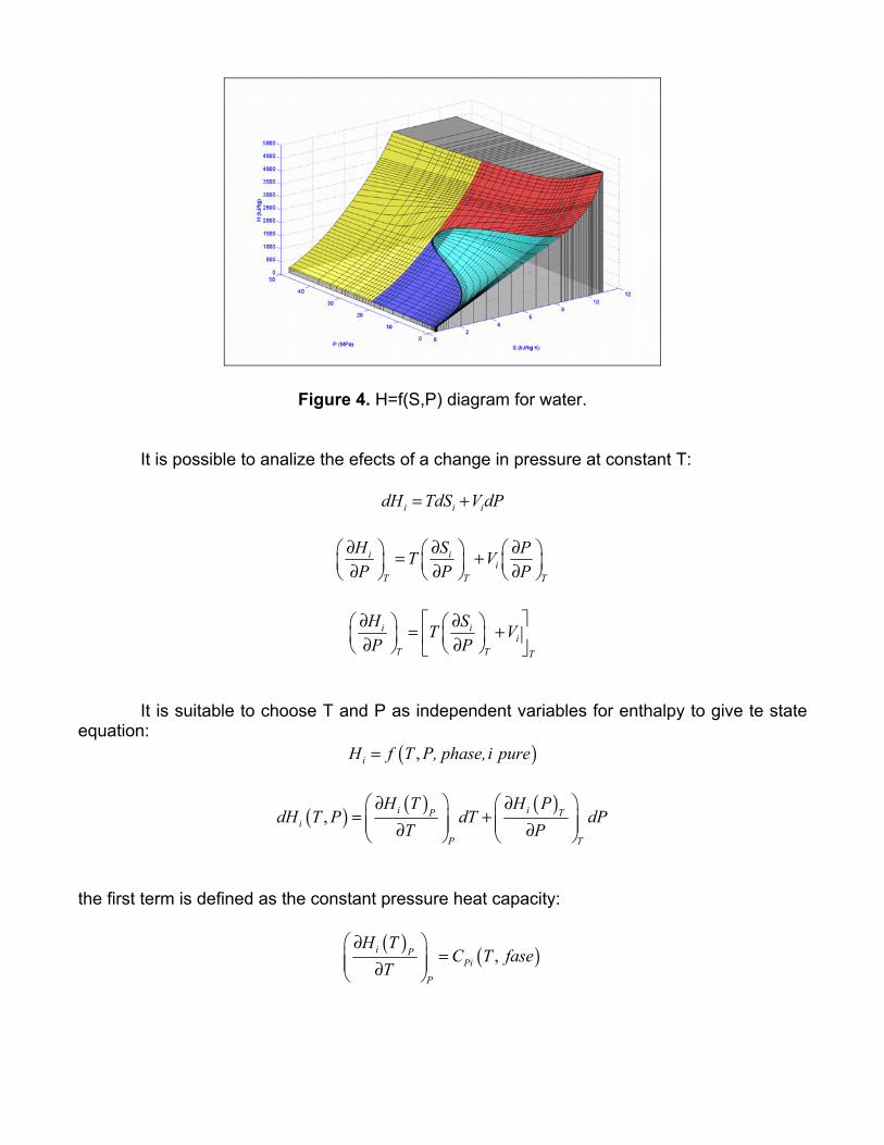
Figure 4. H=f(S,P) diagram for water.

It is possible to analize the efects of a change in pressure at constant T:

i i idH TdS V dP= +

i ii

T T T

H S PT VP P P

∂ ∂ ∂ = + ∂ ∂ ∂

i ii

T T T

H ST VP P

∂ ∂ = + ∂ ∂

It is suitable to choose T and P as independent variables for enthalpy to give te state equation:

( ),iH f T P, phase, i pure=

( ) ( ) ( ), i iP T

i

P T

H T H PdH T P dT dP

T P ∂ ∂

= + ∂ ∂

the first term is defined as the constant pressure heat capacity:

( ) ( ), i PPi

P

H TC T fase

T ∂

= ∂

The study of a change in pressure at constant T leads to analize the effect of pressure in entropy at constant T, with the inconvenient of being a non-measurable or derived property:

( )i iTi

T TT

H P ST VP P

∂ ∂ = + ∂ ∂

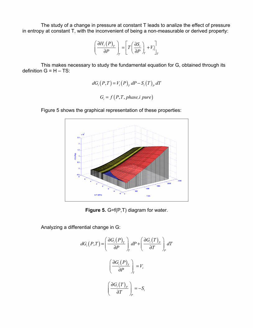
This makes necessary to study the fundamental equation for G, obtained through its definition G = H – TS:

( ) ( ) ( ),i i iT P

dG P T V P dP S T dT= −

( ), , iG f P T phase,i pure= Figure 5 shows the graphical representation of these properties:

Figure 5. G=f(P,T) diagram for water.

Analyzing a differential change in G:

( ) ( ) ( ), i iT P

i

T P

G P G TdG P T dP dT

P T ∂ ∂

= + ∂ ∂

( )i T

i

T

G PV

P ∂

= ∂

( )i P

i

P

G TS

T ∂

= − ∂

2i i

P

G VT P T

∂ ∂ = ∂ ∂ ∂

2

i i

T

G SP T P

∂ ∂ = − ∂ ∂ ∂

it is possible to find the Maxwell relation:

i i

P T

V ST P

∂ ∂ = − ∂ ∂

This Maxwell relation is used to give H as a function of T and P, in terms of measurable variables only:

( )i i iT

i iT PT TT

H P S VT V T V dPP P T

∂ ∂ ∂ = + = − + ∂ ∂ ∂

( ) ( ), , ii Pi i

P T

VdH T P C T fase dT T V dPT

∂ = + − + ∂

The 3D phase diagram associated to the equation of H as a function of P an T is presented in Figure 6:

Figure 6. H=f(T,P) diagram for water.

If the differential of the PV product is used, the equation changes the partial differential

of V for that of P:

( )i

ii i i

P VT T

V PT V dP d PV T P dVT T

∂ ∂ − + = + − ∂ ∂

An analogous analysis can be performed for entropy, using the results obtained to this point. With T and V as selected independent variables:

( ),iS f T V, phase, i pure=

i i iTdS dU PdV= +

( ) ( ) ( ),, ii i T

i i i

P VdU T VdS T V dV

T T= +

as established before:

( ) ( ), ,

i

i i V ii

V T

dU T V C T phase P PdT dVT T T T

∂ = + − ∂

according to the phase rule:

( ), iP f T V , phase, i pure=

the function for entropy gives:

( ) ( ) ( ), ,

i

iV i Ti i i i

V T

P VC T phase P PdS T V dT dV dVT T T T

∂ = + + − ∂

Figure 7 represents the graphical interpretation of these properties:

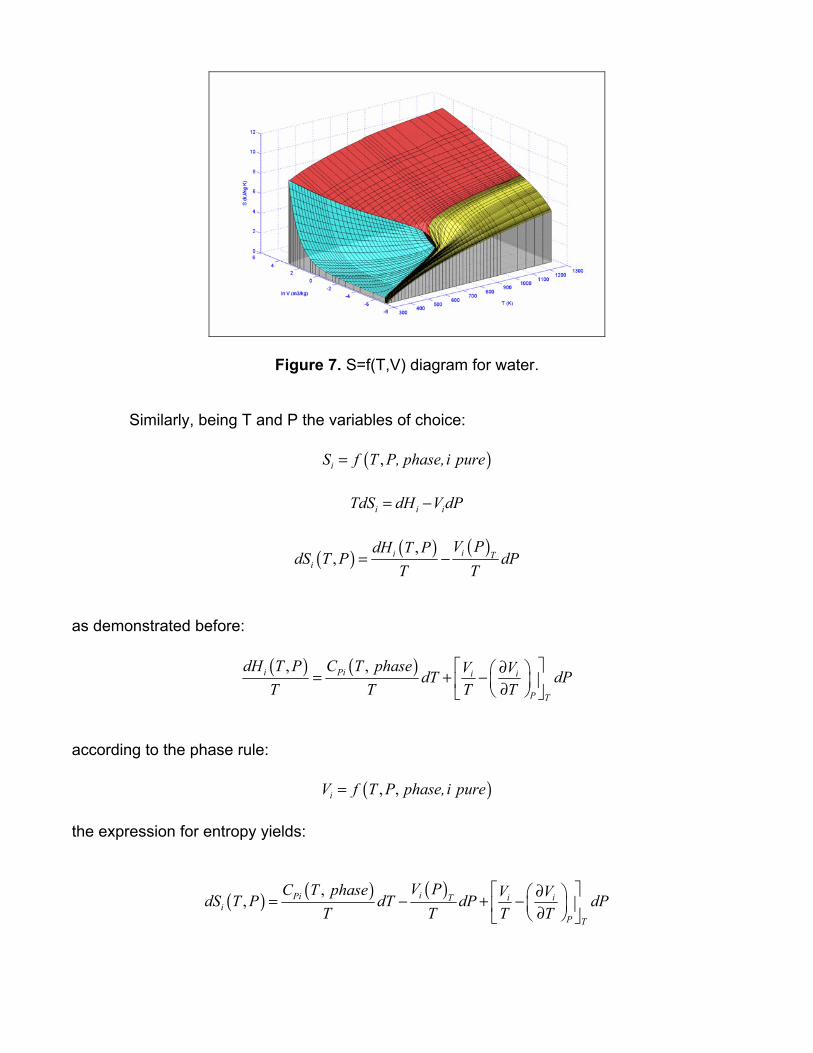
Figure 7. S=f(T,V) diagram for water.

Similarly, being T and P the variables of choice:

( ),iS f T P, phase, i pure=

i i iTdS dH V dP= −

( ) ( ) ( ),, ii T

i

V PdH T PdS T P dP

T T= −

as demonstrated before:

( ) ( ), , i Pi i i

P T

dH T P C T phase V VdT dPT T T T

∂ = + − ∂

according to the phase rule:

( ), ,iV f T P phase, i pure=

the expression for entropy yields:

( ) ( ) ( ), , iPi i iT

iP T

V PC T phase V VdS T P dT dP dPT T T T

∂ = − + − ∂

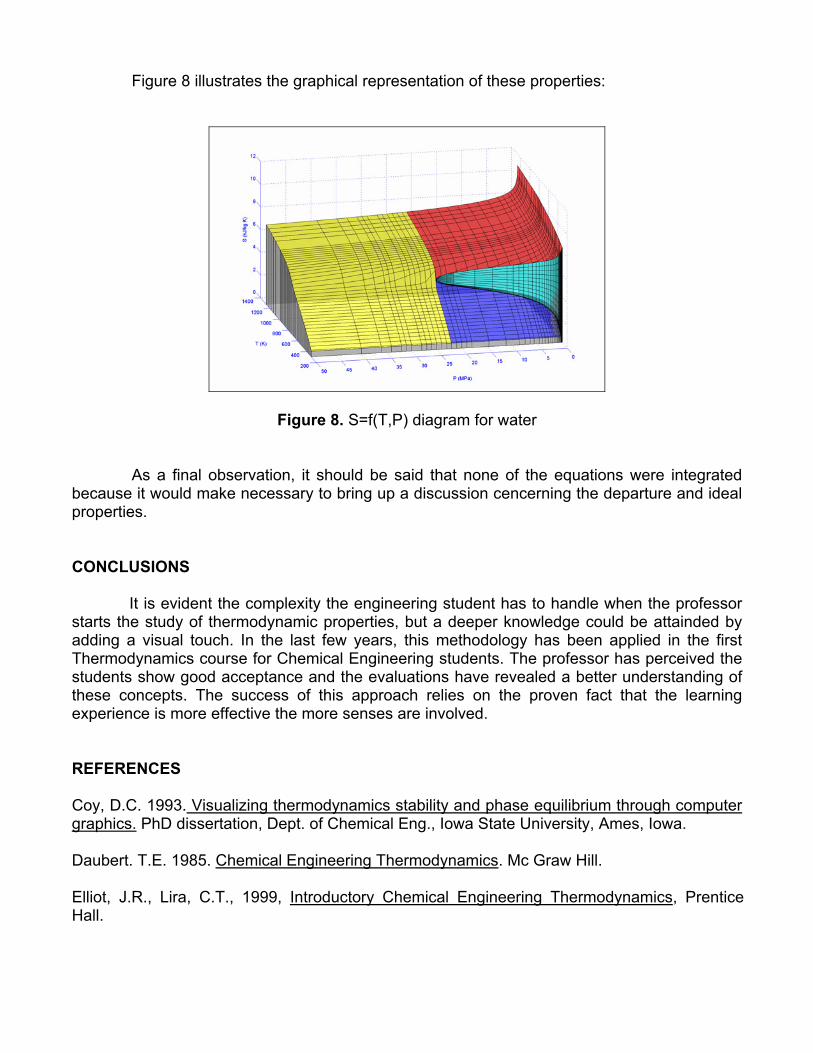
Figure 8 illustrates the graphical representation of these properties:

Figure 8. S=f(T,P) diagram for water

As a final observation, it should be said that none of the equations were integrated because it would make necessary to bring up a discussion cencerning the departure and ideal properties. CONCLUSIONS

It is evident the complexity the engineering student has to handle when the professor starts the study of thermodynamic properties, but a deeper knowledge could be attainded by adding a visual touch. In the last few years, this methodology has been applied in the first Thermodynamics course for Chemical Engineering students. The professor has perceived the students show good acceptance and the evaluations have revealed a better understanding of these concepts. The success of this approach relies on the proven fact that the learning experience is more effective the more senses are involved. REFERENCES Coy, D.C. 1993. Visualizing thermodynamics stability and phase equilibrium through computer graphics. PhD dissertation, Dept. of Chemical Eng., Iowa State University, Ames, Iowa. Daubert. T.E. 1985. Chemical Engineering Thermodynamics. Mc Graw Hill. Elliot, J.R., Lira, C.T., 1999, Introductory Chemical Engineering Thermodynamics, Prentice Hall.

Haar, L., et. al., 1984. NBS/NRC Steam Tables. Hemisphere Publishing Corporation. Jolls, K. 1990. Gibbs and the art of thermodynamics, Proceedings of the Gibbs Symposium,Yale University, New Haven, CT, May 15-17, 1989, p 293-321. Kyle, B.G., 1999. Chemical and Process Thermodynamics, 3rd. edition., Prentice Hall. Márquez, C.E., 2002. Diseño de superficies termodinámicas 3D y de software de predicción de propiedades para compuestos puros. Tesis de Licenciatura, Departamento de Ingeniería Química y Alimentos, Universidad de las Américas, Puebla, México. Prausnitz, J.M., Lichtenthaler, R.N. y Azevedo, E.G., 1999, Molecular Thermodynamics of Fluid-Phase Equilibria, 3rd. edition., Prentice Hall. Ríos, L.G., et. al. 2003. Un paso adelante en la enseñanza del ELV de mezclas binarias: de las matemáticas a las superficies 3D. XXIV Encuentro anual del AMIDIQ. Ixtapa Zihuatanejo, Gro., 13-16 de Mayo de 2003. NOTATION General A Helmholtz free energy CP Constant pressure heat capacity CV Constant volume heat capacity G Gibbs free energy H Enthalpy P Pressure S Entropy T Temperature U Internal energy V Volume Subscripts i Pure component I P Constant pressure T Constant temperature V Constant volume