Understanding European Real Exchange Rates¤

MARIO J. CRUCINIy CHRIS I. TELMERz MARIOS ZACHARIADISx

First draft: June 1998Current draft: January 2003

Abstract

We study good-by-good deviations from the Law-of-One-Price for over 5,000 goods and ser-vices between European Union countries for the years 1975, 1980, 1985 and 1990. We …nd thatbetween most countries there are roughly as many overpriced goods as there are underpricedgoods. Equally-weighted and CPI-weighted averages of good-by-good relative prices generaterelatively accurate predictions of most nominal cross-rates, as purchasing power parity (PPP)would suggest. These …ndings are robust across years, in spite of relatively large movements innominal exchange rates. Variation around the averages is large but is found to be related to eco-nomically meaningful characteristics of goods such as international tradeability, non-tradednessof factors of production and the competitive structure of the markets in which the goods aresold. Using data on product brands, we …nd that product heterogeneity is at least as importantas geography in explaining relative price dispersion. Overall, our data provide strong evidencethat international goods markets are segmented, but (i) the evidence relies on absolute devia-tions from the Law-of-One-Price, not deviations from PPP, (ii) some markets are much moresegmented than others, with the distinctions being consistent with economic theory.

¤The predecessor of this paper circulated as: “What can we learn from deviations from the law of one price?” …rstpresented at the 1998 NBER Summer Institute. In addition to participants at numerous seminars and conferences,we thank Stephen Cosslett, Paul Evans, Burton Holli…eld, Kjetil Storesletten and Stan Zin for helpful comments.We are particularly indebted to Charles Engel who provided many detailed and constructive comments on earlierversions. We gratefully acknowledge the …nancial support of the National Science Foundation (SES-0136979) and theCarnegie Bosch Institute.

yDepartment of Economics, Vanderbilt University; mario.j.crucini@vanderbilt.eduzGraduate School of Industrial Administration, Carnegie Mellon University; chris.telmer@cmu.edu.xDepartment of Economics, Louisiana State University; zachariadis@lsu.edu.

1

1 Introduction

The Law-of-One-Price states that identical goods which are sold in di¤erent countries should have

identical prices, once the prices are expressed in common currency units. Purchasing Power Parity

(PPP) is the notion that this should hold on average, across goods: similar baskets of goods

should cost the same once expressed in common units. Knowing the extent to which data support

these propositions is important for understanding nominal exchange rate behavior, international

industrial organization, the pricing of international …nancial assets, and a host of other questions

in international economics.

Surprisingly, relatively little empirical research has actually tested either of The Law-of-One-

Price or PPP. Instead, most previous work has tested their implication: changes in international

relative prices should equal zero. The main reason has been data limitations. Aside from a handful

of counterexamples, most of the data available outside of the national statistical agencies takes

the form of index numbers.1 Data in the form of absolute prices — prices in dollars, pounds, yen

and so on — has been hard to come by, particularly for the broad baskets of goods and services

required to assess purchasing power. This has been an important impediment to our understanding,

in particular our understanding of the well-known rejections of the propositions in their various

forms. Do we reject PPP because most international goods markets are highly segmented? Or, are

some markets segmented while other markets are integrated, with prices behaving in such a way

that the latter dominate the former?2

Our paper attempts to …ll this void and answer these questions. We use data on retail prices

— prices denominated in local currency units — for a broad set of goods and services in all Europe

1Exceptions are Robert Cumby (1996) who studies Big Mac hamburgers, Kenneth A. Froot, Michael Kim andKenneth Rogo¤ (1995) who study wheat, butter and charcoal, Atish R. Gosh and Holger C. Wolf (1994) who studythe Economist Magazine, Jonathan Haskel and Wolf (1998) who study IKEA furniture, and Mattias Lutz (2001) whostudies automobiles. Recent work by Collin Crownover, John Pippenger and Douglas G. Steigerwald (1996), DavidC. Parsley and Shang-Jin Wei (2000) and John H. Rogers (2001) involve more extensive cross-sections.

2For example, Engel and Rogers (1999) …nd that, across U.S. cities, the variability of changes in relative prices islarger for traded goods than for non-traded goods. Is this evidence of segmented markets? Or are markets for tradedgoods well integrated while prices for non-traded goods just don’t move around very much? As Engel and Rogers(1999) note, it is di¢cult to know without data on absolute price levels. A relatively small amount of (geographic)dispersion in the relative prices of traded goods, for instance, would be supportive of integrated markets for tradedgoods, in spite of the fact that their relative prices might display higher time series volatility than that of non-tradedgoods.

2

Union countries over …ve-year intervals between 1975 and 1990. The data are quite comprehensive,

covering most CPI categories, and are collected with the explicit goal of generating cross-country

comparisons of individual goods and services which are as similar as possible.

We begin by considering the cross-sectional distribution (i.e., good-by-good) of deviations from

The Law-of-One-Price across bilateral country pairs. Using Belgium as the numeraire, we …nd,

somewhat surprisingly, that although the deviations can be very large, they tend to average to zero.

That is, in most countries (relative to Belgium) there tends to be as many overpriced goods as there

are underpriced goods. This phenomenon is robust across all four time periods, in spite of relatively

large swings in nominal exchange rates. Moreover, when we weight the good-by-good deviations

according to CPI expenditure shares — thus constructing the ‘real exchange rate’ in absolute

units — we …nd that deviations from PPP are not large in most cases. The exceptions almost all

involve the relatively poor countries, Spain, Ireland, Greece and Portugal. PPP, therefore, seems

to describe intra-European aggregate prices reasonably well, at least during the years 1975, 1980,

1985 and 1990. Our data provide strong evidence of segmented goods markets but, interestingly,

the evidence is in terms of absolute price dispersion, not deviations from PPP as has been the case

in many previous studies.

The remainder of our paper is dedicated to relating good-by-good, cross-country price dispersion

to the economic characteristics of goods. For example, consider two bottles of beer, one served on

Las Ramblas, in Barcelona, and one served in the Squirrel Hill Cafe, in Pittsburgh. Each good

obviously contains a location-speci…c component: most people have preferences over Barcelona

versus Pittsburgh. Similarly, the production of each good requires non-tradeable inputs such as

labor. On the other hand, beer is an internationally tradeable commodity, suggesting, in addition

to location speci…city, some sort of good-speci…city. We try to understand price dispersion in terms

of the characteristics which might govern where a particular good lies in this location-good space.

We take guidance from a large theoretical literature — including papers by George Alessandria

(1999), Caroline Betts and Timothy Kehoe (1999), Bela Balassa (1964), William J. Baumol and

William G. Bowen (1966), Paul R. Krugman (1987), Paul A. Samuelson (1964), Wilfred J. Ethier

(1979), and Alan C. Stockman and Linda L. Tesar (1995) — which suggests the importance of

tradeability, production structure, the industrial organization of the markets in which the goods

are sold, and so on.

3

We …nd that such theories have much to say about the price dispersion we observe in Europe.

Dispersion among non-tradeable goods is roughly 10% higher than that of tradeables (i.e., dis-

persion of 32% versus 22%). Goods which require lots of non-tradeable inputs to produce exhibit

relatively high dispersion. Combining the two, we …nd that if we consider a non-tradeable good

with the maximum share of non-traded inputs, and compare it to a traded good with the minimum

share of non-traded inputs, cross-country price dispersion falls from 32.6% for the former to 16.8%

for the latter. We also …nd that price dispersion is higher for services and heavily taxed goods such

as alcohol and tobacco, and that identical goods across countries exhibit roughly the same degree

of dispersion as do di¤erentiated goods (di¤erent brands of similar goods) within a country.

Our work is related to an extensive empirical literature that studies the time-series behavior

of nominal and real exchange rates. At the aggregate level, numerous papers have shown that

deviations from PPP based upon consumer price indices can be large and persistent with half

lives in the neighborhood of three to …ve years (see Froot and Rogo¤ (1995) for a survey of this

literature). Much of this literature involves currencies vis-a-vis the U.S. dollar. We …nd that the

story is di¤erent for intra-European real exchange rates. While bilateral real and nominal exchange

rates across the U.S. and individual European countries have been shown to have high positive

correlation and comparable variability, intra-European real exchange rates have considerably lower

variability than nominal exchange rates and the two are actually negatively correlated. We show

that OECD and Penn World Table estimates of real exchange rates tell a similar story.

Another body of papers — including Charles Engel (1993), Engel and Rogers (1996, 1999),

Froot, Kim and Rogo¤ (1995), Alberto Giovannini (1988), Peter Isard (1977), Parsley and Wei

(2000), Rogers and Michael Jenkins (1995) and David C. Richardson (1978) — examine less ag-

gregated prices. They show that economically large deviations from PPP are not a mere artifact

of examining CPI baskets of questionable comparability. International borders seem to represent

something special for the determination of relative prices. The papers by Engel and Engel and

Rogers map this into a geographic metric, and argue that international borders are very ‘wide.’

Their results are based on time-series variation in the prices of similar goods within and across

countries. Our results are based on cross-sectional variation. We show that, for the average good,

cross-country dispersion in the deviation from the Law-of-One-Price is 25%. We also show that,

if real exchange rates are highly persistent, this measure of cross-sectional variance is consistent

4

with Engel and Rogers’ measures of time series variance. We do not have data on intra-European

price dispersion. Parsley and Wei (2000), however, …nd that average absolute dispersion across

U.S. and Japanese cities is roughly 15%. Therefore, a rough measure of border width, based on

cross-sectional variation, is that price dispersion increases (on average) from 15% to 25%.

The remainder of the paper is organized as follows. We begin in Section 2 by describing

the structure and scope of our data. In Section 3 we present some basic descriptive statistics to

illustrate the considerable range of Law-of-One-Price deviations across goods and the tendency for

these deviations to average to zero across goods. We relate this second property of the data to

PPP by weighting our micro-data by consumption expenditure shares. Section 4 contains the main

results of the paper. Here we compute a measure of price dispersion across countries for each good in

our sample and relate this dispersion measure to features of the good. We also explore the potential

for brand di¤erentiation and geographic price discrimination to explain price variance within and

across countries using data on brands. Section 5 concludes with remarks about the implications

of our …ndings for the large and growing theoretical literature on the dynamics of international

relative prices.

2 The Data

The original source of our price data is a series of publications by Eurostat, the statistical agency of

the European Community, each containing the results of an extensive retail price survey conducted

in various capital cities of Europe.3 Table 1 presents basic information about what our cross-

sections entail. We have detailed retail prices at …ve year intervals between 1975 and 1990. In 1975

the survey covers nine European countries, in 1980 Greece, Portugal and Spain are added while in

1985 Austria is added. The number of goods included in the survey also grows over time from 658

items in 1975 to 1,896 items in 1990.

As Table 1 indicates there are a great number of missing observations in the price surveys,

13% are missing in 1975 and the number increases abruptly in 1980 to 36% and remains at about

that level. The number of missing observations di¤ers systematically across countries from a low

of about 9% to a high of about 55%. Belgium is consistently the country with the fewest missing3Exceptions are the survey data for Germany and the Netherlands in 1980, 1985 and 1990 in which case the prices

are averages across cities within each country.

5

observations while Ireland is consistently the country with the most missing observations.

Since our main focus is on explaining price dispersion across countries we eliminate any good

which has an insu¢cient number of cross-country observations, which we de…ne as 4 in 1975, 5

in 1980, and 6 in 1985 and 1990. The increments to our criteria re‡ect the fact that the number

of countries in the sample increases over time. We also control for gross measurement error by

eliminating goods for which the common-currency price di¤ers from the good-speci…c median by

a factor of 5 or more. These …lters reduce our sample of goods from a total of 5,449 to 3,545

with the details for individual years provided in Panel B of Table 1. Of these remaining data, the

proportion of missing observations never exceeds 25%. For calculations which require a numeraire

to be de…ned, we use Belgium for the simple reason that it has the fewest missing observations.

Our survey data also contain a large number of brand-name goods, typically accounting for about

one-third of the goods that we utilize.

Table 2 reports a number of individual records from the 1985 survey with the goods chosen to

be representative of the various overall categories contained in our dataset. All the surveys have a

similar structure involving a Eurostat code, a detailed description of the particular good, the units

of measure and columns of price data. The retail prices are cash prices paid by …nal consumers

and therefore will include taxes, such as VAT. The prices are themselves averages of the surveyed

prices across di¤erent city-wide sales points.4

As is evident from the sample of goods reported in this table, the surveys are as comprehensive

as those used to construct national consumer price indices. In the sample presented we see food

items, clothing, major appliances, automobiles, services, and so on. Although Eurostat reports the

prices in local currency units, Table 1 presents prices in Belgian francs to facilitate comparisons.

The deviations we see from the Law-of-One-Price are suggestive of what is to come. The rental

cost of a television, for instance, varies widely across countries whereas the dispersion in the cost

of rice is much smaller.

The descriptions that Eurostat publishes are abbreviated versions of those used by the statistical

agency to compile the data. The level of detail in the published version also varies across goods.

In particular, goods can be placed into two categories: those indicated as selected brands (s.b. in

4The procedure for selecting sales points follows the practice used to construct national consumer price indices.Sales points are selected by the national statistical o¢ces so that the sample is representative of the distribution ofprices in the city with more observations collected for goods having greater price dispersion within the city.

6

Table 2) and those without such a designation. The reason given for the selected brand designation

is the need for con…dentiality. While we might like to know which automobiles are Mercedes and

which are Volvos the record does not provide us with the necessary details. However, the survey is

explicitly designed to assure comparability of goods across locations.

One last important issue regarding the price data is the exact timing of the surveys. While we

…nd it convenient to refer to our cross-sections by year, in reality the price data for each cross-

section is collected in a sequence of surveys. The nominal exchange rate data with which we convert

prices into a common currency takes explicit account of this timing, taking the form of averages of

daily data over the relevant time intervals.

Much of our paper attempts to relate international price dispersion to economically meaningful

characteristics of goods. Toward this end, we supplement our retail price data with information

on trade and production structure. Because these variables are unavailable at the level of the

individual good we assign each good to an industry and use the industry-level measure in place of

the good-speci…c measure.

We de…ne tradeability of a good as the ratio of the total trade among the countries in our

sample in a particular industry divided by total output of that industry across the same countries.5

Among traded goods, the trade shares range from a low of 15.1% for printing, publishing and allied

industries to a high of 129.5% for professional goods (see Table 3). The average trade share is very

substantial, equalling 54.3%.

We also consider the share of non-traded inputs into the production of a good. We de…ne

this as the ratio of non–traded inputs to total cost where both numbers are computed from the

1988 input-output tables of the United Kingdom.6 Table 4 contains the cost share of non-traded

intermediate inputs by industry. The values range from a low of 4.6% for tobacco to a high of

31.8% for forestry and …sheries.

Comparing some of the numbers in Table 3 and 4 it is obvious that the distinction between

tradeability and trade in ‘middle products’ is important. As is often asserted, all retail goods involve5We use the actual trade share whenever trade data is available and assign an index of zero otherwise. The

industries assigned zero trade shares are: restaurants and hotels, transport, storage and communication, inlandtransport, maritime transport, communication, …nancing, insurance, real estate and community, social and personalservices.

6Non-traded inputs are assumed to include: utilities, construction, distribution, hotels, catering, railways, roadtransport, sea transport, air transport, transport services, telecommunications, banking, …nance, insurance, businessservices, education, health and other services.

7

signi…cant amounts of non-traded inputs (the cross-industry average share of non-traded inputs is

14.1%). Less well appreciated is the fact that all non-traded goods involve some traded inputs.

From an economic standpoint it is unclear whether a ‘non-traded’ good with substantial traded

inputs will exhibit more or less price dispersion than a ‘traded good’ with substantial non-traded

inputs. Our analysis is explicitly designed to separately identify these two economic e¤ects.

3 Deviations From the Law-of-One-Price

We denote pij as the local currency price of good i in country j. The numeraire country is denoted

n and the nominal exchange rate for country j’s currency in units of country n’s is ej . We de…ne

qij = log(ejpij=pin), as the law-of-one-price deviation for good i between country j and n. If qij is

positive, good i is more expensive in country j than country n, the numeraire.

Figure 1 summarizes the empirical distribution of deviations from the Law-of-One-Price. The

…gure contains one chart for each country for which we have four cross sections of data. Each chart

reports four kernel estimates of the density of qij, one estimate for each of the 1975, 1980, 1985

and 1990 cross sections. The numeraire is Belgium. The chart in the lower right corner pools all

countries together, thus characterizing the distribution of all prices (across goods and countries)

relative to Belgium.

Figure 1 exhibits three striking features. First, most of the densities are centered at zero. That

is, there are roughly as many overpriced goods as there are underpriced goods in a given country

compared to Belgium. Second, this phenomenon is relatively stable over time. In spite of relatively

large movements in nominal exchange rates over the period, the location of the density estimates

doesn’t move around very much. Finally, the variance of law-of-one-price deviations across goods

is large, with the support of many of the densities being on the order of plus or minus 150%.7

The …rst feature – the locations of the densities – suggests that law-of-one-price violations

average out in the aggregate. Table 5 reports the estimated means and their standard errors. For

most countries and time periods the average law-of-one-price deviation is statistically di¤erent from

7Luxembourg, which has a …xed exchange rate with Belgium, is an interesting special case. Figure 1 shows thatdispersion is substantially smaller for Luxembourg than for the remaining countries. In 1985, for example, roughly40% of Luxembourg’s prices were within 10% of those from Belgium, whereas only 20% (on average) satisfy the samecriteria for the other countries. While geographical distance might seem a likely reason, it’s important to note thatLuxembourg is roughly as close to Brussels as it is to Amsterdam and Paris. This points to the nominal exchangerate regime as an obvious candidate for explaining the cross-country di¤erences.

8

zero, however the di¤erences are often quite small. In 24 of 32 cases the average is less than 10% in

absolute value (we ignore the poor countries in Table 5 for now). If we exclude Denmark — which

has a relatively high VAT — this is true for 24 of 28 cases.

The fact that there are roughly as many overpriced as underpriced goods, and that this persists

over time, is interesting. It suggests that, over …ve year periods, changes in nominal exchange rates

do not simply shift the distribution of relative prices around. It is also suggestive of purchasing

power parity. In the next section we examine the latter more closely.

3.1 Purchasing Power Parity

The right-most columns of Table 5 ask to what extent our data indicate that CPI-type baskets of

goods cost the same in di¤erent locations. This is accomplished by taking consumption expenditure-

weighted averages of the good-by-good real exchange rates depicted in Figure 1.8 For the most

part, we see only minor di¤erences between the expenditure-share weighted and equally weighted

PPP measures. The mean absolute deviation between the two is just 4.5% and only four values

di¤er by more than 10% (Portugal in 1980 and 1985, and Greece in 1980 and 1990). The reasons

are (i) the two weighting schemes are not as di¤erent as one might think (e.g., perishable goods are

purchased often but cost little, whereas durable goods are purchased infrequently and cost a lot),9

and (ii) there is little tendency in our data for large expenditure share goods to be systematically

over or under-valued.

CPI weighting, therefore, tells much the same story as equal weighting discussed in the previous

section. Denmark is roughly 20% more expensive than Belgium in all years. Purchasing power never

deviates by more than 10% across Austria, France, Germany, and Luxembourg while the deviations

from PPP in Ireland, Italy, the Netherlands, and the United Kingdom exceed 10% in only a single

year. In contrast, price levels in Greece, Portugal and Spain are substantially lower than Belgium,

ranging from 14% to 46% lower depending on the country and time period.

Table 5 suggests two candidates for interpreting what we observe. First, the table lists countries8Speci…cally, if we denote the average expenditure share on good i between countries j and n as wi, then the

relative cost of the aggregate consumption basket (in percent) isP

i wi(ejpij=pin) ¡ 1. Our analysis is based onPi wiqij , which is approximately the same (and has the usual statistical bene…ts). Data on consumption expenditure

shares are taken from the International Comparison Project. Further details are given in the data appendix.9For example, the 1990 German price index gives a weight of 2.4% to “meat and …sh” and a weight of 2.6% to

passenger automobiles.

9

by income level, from highest to lowest. Consistent with many previous papers — the pioneering

work of Irving B. Kravis and Robert E. Lipsey (1983) for instance — the poorer countries clearly

tend to have lower price levels. The correlation between price levels and income is roughly -

0:80 regardless of the year or measure used. Second, the table documents the year of entry into

the European Union, the idea being that the poorer countries entered the European Union later

and should be expected to have di¤erent relative prices. There are, however, two problems with

this explanation. First, if trade barriers were the explanation we would expect convergence in real

exchange rates across the original members and late entrants and there is no evidence of this in Table

5. Second, if we compute real exchange rates across traded and non-traded goods the di¤erences

are much larger for non-traded goods than for traded goods, consistent with the Balassa-Samuelson

hypothesis. Table 6 presents additional evidence related to this last point, breaking down our real

exchange rate estimates into traded and non-traded goods. We see that most of the variation across

countries is due to variation in non-traded goods prices, not traded goods prices. This pattern is

evident for each time period and each country. There is also some evidence of convergence over

time for traded goods, particularly from 1975 to 1985. A natural explanation is the elimination

of formal tari¤ barriers across member countries and the quadrupling of intra-EU trade over the

period.

3.2 Relationship with Other Evidence

An important issue is the extent to which our results and data are consistent with previous work

and alternative datasets. This section addresses this using absolute price data from the OECD and

Penn World Tables (PWT) as well as the more commonly-used national CPI index number data.

We focus on the properties of the aggregate, CPI-weighted real exchange rates as in Table 5.

Beginning with absolute price data, Figure 2 organizes countries by income level and then plots

our real exchange rate estimates (from Table 5) and their con…dence intervals alongside analogous

estimates from the OECD. In spite of the cross-section of goods and services being quite di¤erent

(at least conceivably), we see that in many cases the real exchange rates are quite similar. The

pairwise, mean absolute deviation is 7% and the correlation is 0.85. The …gure also reiterates the

main message of Table 5; deviations from PPP are often quite small for high income countries and

there is a negative correlation between price levels and national income.

10

Turning to CPI index-number data, any comparison must be in terms of time-series properties.

That is, we must transform our data from absolute units into changes. We focus on the prominent

…nding of Mussa (1986), who concluded that the correlation between changes in nominal exchange

rates and CPI-based real exchange rates is very high, on the order of 0.90. Mussa’s data frequency

was quarterly. Our Eurostat data is available only at the …ve-year interval, so direct comparisons

are obviously limited. We can, however, ask two questions. First, the alternative sources for

absolute prices — the OECD and PWT data — are available annually. We can therefore compare

changes in these data to changes in CPI data (implicitly, Mussa’s data), and rely on the fact that

the Eurostat data seem quite similar to the OECD data (Figure 2). Second, we can simply make

comparisons at the …ve-year frequency.

Table 7 examines annual changes. The table shows correlations between changes in (log) nominal

and CPI-based real exchange rates using three di¤erent numeraires — the U.S., Belgium and

Germany — as well as the average correlation across all possible numeraires. It also shows the

implications of PWT and OECD data. By and large, the story is a somewhat muted version of

Mussa’s. The correlations are all in the range of 0.65 to 0.78. There does not appear to be a strong

numeraire e¤ect with the exception of the U.S., which increases the correlation from roughly 0.70

to 0.80.

Table 8 examines …ve-year changes. The correlations are uniformly lower than their annual

counterparts, sometimes by a substantial amount. Most notably, the Eurostat sample generates

values which are roughly zero and this is consistent across data-sources. Incorporating the missing

time periods (Row 2) increases the correlations, but they are still relatively low compared to the

sample which includes the U.S.. At the …ve-year frequency, then, the U.S. data has a substantial

positive e¤ect which is less apparent at the annual frequency. This is a feature of both the CPI

data and the absolute-price data, so the di¤erence cannot be easily attributed to non-comparable

CPI baskets between the U.S. and Europe.

To summarize, we take two lessons from this section. First, at the …ve-year frequency, nominal

and real exchange rates are less correlated within Europe than between Europe and the U.S..

Second, and more important for this paper, a consistency check on our data is satis…ed. The

Eurostat data appear quite consistent with alternative data sources in terms of real exchange rate

behavior. This is encouraging for the main focus of our paper: dispersion in the relative prices

11

which make up the (aggregate) real exchange rate.

4 Understanding International Price Dispersion

The basic building block of our measure of international price dispersion is the percentage deviation

of the price of good i in country j from the cross-country average price of the same good:

zij =ejpijpi

¡ 1; (1)

where pi ´PMij=1 ejpij=Mi and Mi is the number of countries for which we have price observations

on good i. This measure of the deviation from the Law-of-One-Price is independent of the numeraire,

Belgium, for which e = 1. We measure the cross-country price dispersion of good i as,

yi = mad(zij); (2)

where mad(¢) is the mean absolute deviation, which is less sensitive to large outliers than thestandard deviation. The vector, y, of mean absolute price deviations, good-by-good, is what we

seek to explain.

4.1 Descriptive Statistics

Figure 3 summarizes the empirical distributions of our dispersion measure, good-by-good. Each line

in the …gure is a kernel estimate of the density of yi for one of the annual cross-sections. Focusing

on the 1980, 1985 and 1990 cross sections – for which we have basically the same cross-section of

countries – the distributions look very similar, both in location and shape.10

The location of these densities tells us something interesting about the overall importance of

national borders for price dispersion. Consider the hypothesis that the countries in our sample con-

stitute a ‘common market.’ If this were literally true we would expect the densities to be located

near the origin – how close is di¢cult to say, but existing estimates of intranational price disper-

sion provide a valuable benchmark. David Parsley and Shang-Jin Wei (2000) estimate that price

dispersion across cities within Japan and the United States equalled 13% and 14.5%, respectively

in 1985. The average amount of price dispersion in our European sample in the same year is 24.2%.

One explanation for the higher dispersion of international relative prices compared to that ob-

served within countries is exchange rate variability in the presence of prices that are sticky in10The lower dispersion for 1975 is largely due to the omission of Greece, Portugal and Spain from the cross section.

12

domestic currency terms, another is higher arbitrage costs internationally compared to intrana-

tionally. Because the sticky-price explanation does not rely on heterogeneity in price dispersion

across individual goods, we can evaluate its explanatory power as a ‘country e¤ect’ in accounting

for variation in the variables zij from equation (1). For example, the deutschemark appreciated

against the Belgian franc by 25% between 1980 and 1985. If all nominal prices in Germany are

…xed, then all of the percentage deviations, ziG, will increase by 25 percent and all of the variation

relative to other countries will be attributable, not to good-speci…c factors, but to the German

country factor alone. Table 9 shows that while these country e¤ects are economically important,

they explain only between 10 and 20 percent of the variation in our data. Moreover, this number

will tend to overstate country e¤ects due to nominal exchange rate movements once we control for

the wealth e¤ects discussed in Section 3.

Table 10 reports the conditional mean of price dispersion for various types of goods. When

we treat goods as being either traded or non-traded we …nd price dispersion for non-traded goods

is considerably higher, 32.9% compared to only 22.9% for traded goods (using 1985 results). We

also see that price dispersion is 5.8% higher for goods that utilize more than the average amount

of non-traded inputs, 29.2% versus 23.4%. One unexpected …nding is that branded goods exhibit

substantially less price dispersion than non-branded goods, 20.1% compared to 26.2%.

While the broad implications of Table 10 will hold up to further scrutiny in the next section,

we stress the limitations of drawing conclusions from the conditional means alone. One obvious

problem is that the groupings are not mutually exclusive. For example, traded goods also tend to

be goods with lower than average non-traded input shares. Are the conditional means for these two

categorizations really picking up independent sources of variation? We also observe that branded

goods have much higher trade shares than non-branded goods. Do branded goods really have

less price dispersion than non-branded goods or are we picking up the impact of tradeability yet

again? We deal with these issues by adopting a formal regression framework and by separating our

analysis into two parts. The …rst part analyzes the relationship between price dispersion and the

characteristics of goods and the second focuses on market structure using only our brand data.

13

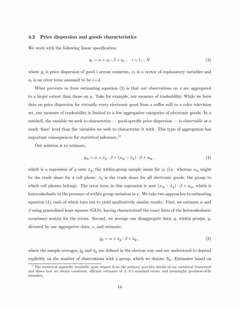
4.2 Price dispersion and goods characteristics

We work with the following linear speci…cation:

yi = ®+ xi ¢ ¯ + ui , i = 1; :::N (3)

where yi is price dispersion of good i across countries, xi is a vector of explanatory variables and

ui is an error term assumed to be i.i.d.

What prevents us from estimating equation (3) is that our observations on x are aggregated

to a larger extent than those on y. Take for example, our measure of tradeability. While we have

data on price dispersion for virtually every electronic good from a co¤ee mill to a color television

set, our measure of tradeability is limited to a few aggregative categories of electronic goods. In a

nutshell, the variable we seek to characterize — good-speci…c price dispersion — is observable at a

much ‘…ner’ level than the variables we seek to characterize it with. This type of aggregation has

important consequences for statistical inference.11

Our solution is to estimate,

yig = ®+ ¹xg ¢ ¯ + (xig ¡ ¹xg) ¢ ¯ + uig ; (4)

which is a regression of y onto ¹xg, the within-group sample mean for xi (i.e. whereas xig might

be the trade share for a cell phone, ¹xg is the trade share for all electronic goods, the group to

which cell phones belong). The error term in this regression is now (xig ¡ ¹xg) ¢ ¯ + uig, which isheteroskedastic in the presence of within group variation in x. We take two approaches to estimating

equation (4), each of which turn out to yield qualitatively similar results. First, we estimate ® and

¯ using generalized least squares (GLS), having characterized the exact form of the heteroskedastic

covariance matrix for the errors. Second, we average our disaggregate data, y, within groups, g,

dictated by our aggregative data, x; and estimate,

¹yg = ®+ ¹xg ¢ ¯ + ¹ug ; (5)

where the sample averages, ¹yg and ¹ug are de…ned in the obvious way and are understood to depend

explicitly on the number of observations with a group, which we denote Ng. Estimates based on

11The statistical appendix (available upon request from the authors) provides details of our statistical frameworkand shows how we obtain consistent, e¢cient estimates of ¯, it’s standard errors, and meaningful goodness-of-…tmeasures.

14

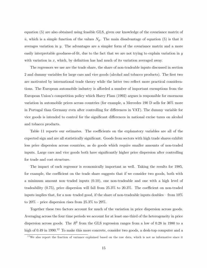
equation (5) are also obtained using feasible GLS, given our knowledge of the covariance matrix of

¹u, which is a simple function of the values Ng. The main disadvantage of equation (5) is that it

averages variation in y. The advantages are a simpler form of the covariance matrix and a more

easily interpretable goodness-of-…t, due to the fact that we are not trying to explain variation in y

with variation in x, which, by de…nition has had much of its variation averaged away.

The regressors we use are the trade share, the share of non-tradeable inputs discussed in section

2 and dummy variables for large cars and vice goods (alcohol and tobacco products). The …rst two

are motivated by international trade theory while the latter two re‡ect more practical considera-

tions. The European automobile industry is a¤orded a number of important exemptions from the

European Union’s competition policy which Harry Flam (1992) argues is responsible for enormous

variation in automobile prices across countries (for example, a Mercedes 190 D sells for 36% more

in Portugal than Germany even after controlling for di¤erences in VAT). The dummy variable for

vice goods is intended to control for the signi…cant di¤erences in national excise taxes on alcohol

and tobacco products.

Table 11 reports our estimates. The coe¢cients on the explanatory variables are all of the

expected sign and are all statistically signi…cant. Goods from sectors with high trade shares exhibit

less price dispersion across countries, as do goods which require smaller amounts of non-traded

inputs. Large cars and vice goods both have signi…cantly higher price dispersion after controlling

for trade and cost structure.

The impact of each regressor is economically important as well. Taking the results for 1985,

for example, the coe¢cient on the trade share suggests that if we consider two goods, both with

a minimum amount non–traded inputs (0.10), one non-tradeable and one with a high level of

tradeability (0.75), price dispersion will fall from 25.3% to 20.3%. The coe¢cient on non-traded

inputs implies that, for a non–traded good, if the share of non-tradeable inputs doubles – from 10%

to 20% – price dispersion rises from 25.3% to 29%.

Together these two factors account for much of the variation in price dispersion across goods.

Averaging across the four time periods we account for at least one-third of the heterogeneity in price

dispersion across goods. The R2 from the GLS regression ranges from a low of 0.28 in 1980 to a

high of 0.49 in 1990.12 To make this more concrete, consider two goods, a desk-top computer and a

12We also report the fraction of variance explained based on the raw data, which is not as informative since it

15

haircut. Based on our measures, these particular goods have very di¤erent economic characteristics.

A desk-top computer, being drawn from the o¢ce, computing and accounting machinery sector,

has a high trade share and a low non-traded input share. In contrast, a haircut, being drawn

from the community, social and personal service sector, is a non-traded good with a high share

of non-traded inputs into production. Based on our regression model, if we move from a desk-top

computer to a haircut, price dispersion is predicted to double, rising from 16.8% to 32.6%.

In summary, we …nd that theories distinguishing goods by the extent of their tradeability and

the transformation of traded goods to …nal goods account for a signi…cant fraction of cross-country

price dispersion. The last factor we consider is market structure.

4.3 Price dispersion and market structure

Arthur Pigou (1920) de…ned price discrimination as being present when di¤erent groups of con-

sumers pay di¤erent prices for identical goods. In the “pricing to market” literature (see Krugman

(1995) and Robert C. Feenstra (1995) for comprehensive reviews) price discriminating oligopolistic

suppliers use their market power to sustain price di¤erences across national boundaries. Identi-

cal goods, then, could sell at di¤erent prices across countries even when converted to a common

currency. Alternatively, the goods might not actually be identical in which case monopolistically

competitive …rms could charge di¤erent prices depending on the elasticity of substitution between

them. Assuming that international goods are homogenous when in fact they are di¤erent vari-

eties of the same good would, under monopolistic competition, lead to unfounded rejections of the

Law-of-One-Price.

Our panel data is su¢ciently rich that we can shed light on these two alternative views of

the microeconomic structure of goods markets. The procedure boils down to a two-way analysis

of variance. The …rst dimension of the variance captures price di¤erences across brands of the

same good within a country. We refer to these as brand e¤ects: the price di¤erences domestic

consumers pay for di¤erentiated brands of the same good. The second dimension captures the

di¤erences in price of the same brand across countries. We refer to these as country e¤ects: the

price di¤erences international consumers pay for identical brands of a particular good. We gauge

the relative importance of product heterogeneity and geographic price discrimination by comparing

primarily re‡ects the di¤erent levels of aggregation of the regressors and regressand.

16

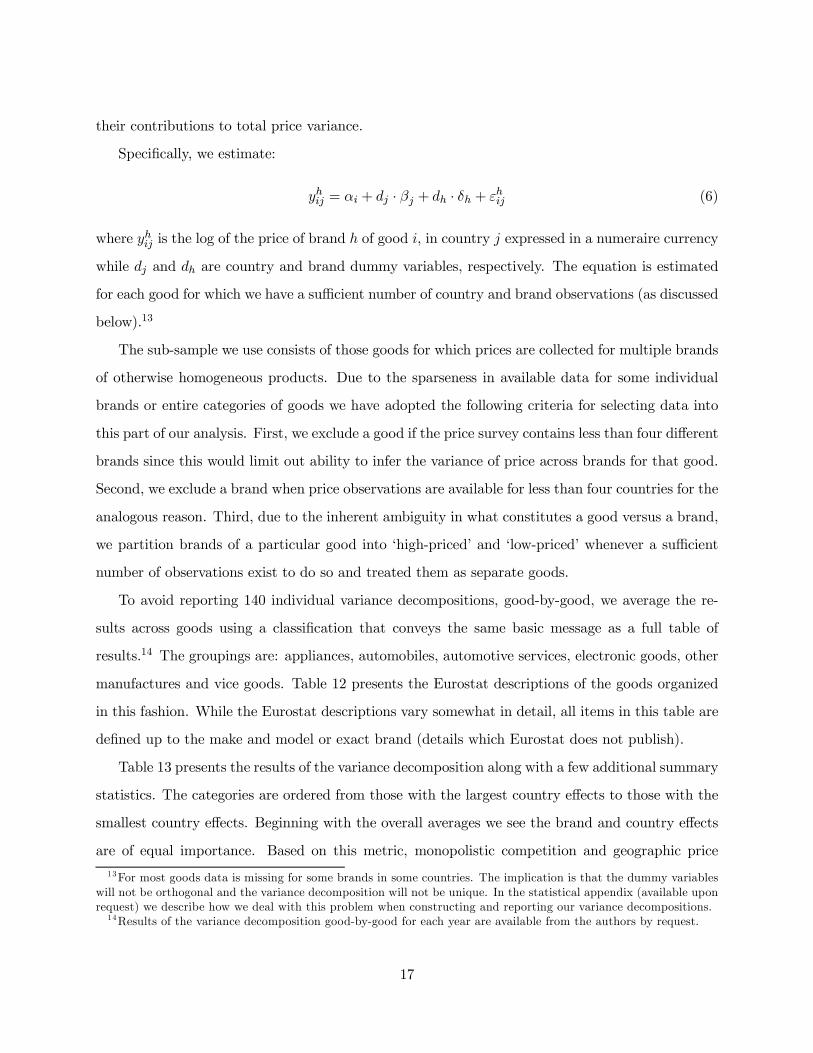
their contributions to total price variance.

Speci…cally, we estimate:

yhij = ®i + dj ¢ ¯j + dh ¢ ±h + "hij (6)

where yhij is the log of the price of brand h of good i, in country j expressed in a numeraire currency

while dj and dh are country and brand dummy variables, respectively. The equation is estimated

for each good for which we have a su¢cient number of country and brand observations (as discussed

below).13

The sub-sample we use consists of those goods for which prices are collected for multiple brands

of otherwise homogeneous products. Due to the sparseness in available data for some individual

brands or entire categories of goods we have adopted the following criteria for selecting data into

this part of our analysis. First, we exclude a good if the price survey contains less than four di¤erent

brands since this would limit out ability to infer the variance of price across brands for that good.

Second, we exclude a brand when price observations are available for less than four countries for the

analogous reason. Third, due to the inherent ambiguity in what constitutes a good versus a brand,

we partition brands of a particular good into ‘high-priced’ and ‘low-priced’ whenever a su¢cient

number of observations exist to do so and treated them as separate goods.

To avoid reporting 140 individual variance decompositions, good-by-good, we average the re-

sults across goods using a classi…cation that conveys the same basic message as a full table of

results.14 The groupings are: appliances, automobiles, automotive services, electronic goods, other

manufactures and vice goods. Table 12 presents the Eurostat descriptions of the goods organized

in this fashion. While the Eurostat descriptions vary somewhat in detail, all items in this table are

de…ned up to the make and model or exact brand (details which Eurostat does not publish).

Table 13 presents the results of the variance decomposition along with a few additional summary

statistics. The categories are ordered from those with the largest country e¤ects to those with the

smallest country e¤ects. Beginning with the overall averages we see the brand and country e¤ects

are of equal importance. Based on this metric, monopolistic competition and geographic price

13For most goods data is missing for some brands in some countries. The implication is that the dummy variableswill not be orthogonal and the variance decomposition will not be unique. In the statistical appendix (available uponrequest) we describe how we deal with this problem when constructing and reporting our variance decompositions.14Results of the variance decomposition good-by-good for each year are available from the authors by request.

17

discrimination are of comparable importance in accounting for price dispersion. However, the

averages are not very representative of the results for the underlying categories. At one extreme,

we see vice goods and automotive services, both with virtually all of the price variation accounted

for by country e¤ects (80% when we average across years). At the opposite end of the continuum

are appliances where the bulk of price variation comes in the form of brand di¤erentiation.

In the case of vice goods, we suspect that most of the country e¤ect is due to variation in national

excise taxes across countries. The large country e¤ect for automotive services is exactly what we

would expect for a classic non-traded good. Among manufactured goods, automobiles are of interest

for a number of reasons. First, the automobile industry has attracted a great deal of interest in the

international trade literature that studies the pass-through of exchange rate ‡uctuations to trade

prices from source to destination markets. Knettner (1989, 1993) …nds more evidence of pricing

to market in the automobile industry than in others that he studies. Interestingly, automobiles

are the last category of goods in Table 13 where country e¤ects dominate brand e¤ects. The large

country e¤ects cannot be dismissed as re‡ecting di¤erences in excise taxes or trade barriers. These

factors do play a role, but only for particular countries and import sources. For example, Flam

(1992) emphasizes very high value-added taxes on automobiles in the case of Denmark and Greece,

and import restrictions imposed on Japanese models by Portugal and the United Kingdom.15 Most

likely, the European automobile industry has large country e¤ects because it is allowed exemptions

from EU competition policy that are not enjoyed by other industries represented in our table.

Of the remaining categories, there is little to distinguish electronic goods from other manufac-

tures. Both categories have considerable amounts of price variation across brands within countries

and across countries for a given brand. Appliances, as one might expect, have the largest brand

e¤ects.

We conclude that the ability of …rms to price discriminate across countries is no greater than

their ability to di¤erentiate their products within a country. When this conclusion fails to hold, we

can point to other factors that account for the di¤erence: in the case of vice goods, excise taxes;

in the case of services, no trade; in the case of automobiles, a combination of factors (excise taxes,

import restraints, and exemptions from EU competition policy).

15See also Lutz (2001) for a very detailed and interesting study of automobile price dispersion in Europe by makeand model.

18

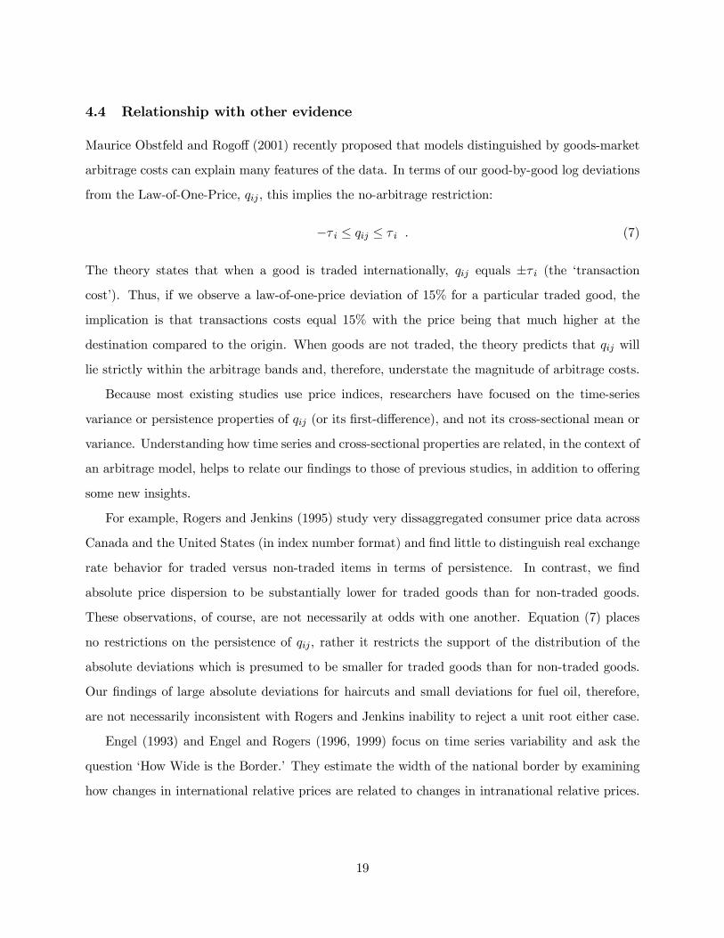
4.4 Relationship with other evidence

Maurice Obstfeld and Rogo¤ (2001) recently proposed that models distinguished by goods-market

arbitrage costs can explain many features of the data. In terms of our good-by-good log deviations

from the Law-of-One-Price, qij , this implies the no-arbitrage restriction:

¡¿ i · qij · ¿ i : (7)

The theory states that when a good is traded internationally, qij equals §¿ i (the ‘transactioncost’). Thus, if we observe a law-of-one-price deviation of 15% for a particular traded good, the

implication is that transactions costs equal 15% with the price being that much higher at the

destination compared to the origin. When goods are not traded, the theory predicts that qij will

lie strictly within the arbitrage bands and, therefore, understate the magnitude of arbitrage costs.

Because most existing studies use price indices, researchers have focused on the time-series

variance or persistence properties of qij (or its …rst-di¤erence), and not its cross-sectional mean or

variance. Understanding how time series and cross-sectional properties are related, in the context of

an arbitrage model, helps to relate our …ndings to those of previous studies, in addition to o¤ering

some new insights.

For example, Rogers and Jenkins (1995) study very dissaggregated consumer price data across

Canada and the United States (in index number format) and …nd little to distinguish real exchange

rate behavior for traded versus non-traded items in terms of persistence. In contrast, we …nd

absolute price dispersion to be substantially lower for traded goods than for non-traded goods.

These observations, of course, are not necessarily at odds with one another. Equation (7) places

no restrictions on the persistence of qij, rather it restricts the support of the distribution of the

absolute deviations which is presumed to be smaller for traded goods than for non-traded goods.

Our …ndings of large absolute deviations for haircuts and small deviations for fuel oil, therefore,

are not necessarily inconsistent with Rogers and Jenkins inability to reject a unit root either case.

Engel (1993) and Engel and Rogers (1996, 1999) focus on time series variability and ask the

question ‘How Wide is the Border.’ They estimate the width of the national border by examining

how changes in international relative prices are related to changes in intranational relative prices.

19

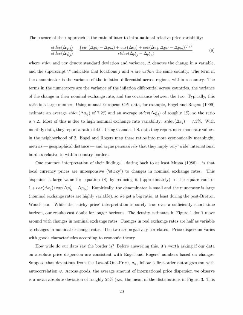
The essence of their approach is the ratio of inter to intra-national relative price variability:

stdev(¢qij)

stdev(¢q0ij)=fvar(¢pij ¡¢pin) + var(¢ej) + cov(¢ej;¢pij ¡¢pin)g1=2

stdev(¢p0ij ¡¢p0in)(8)

where stdev and var denote standard deviation and variance, ¢ denotes the change in a variable,

and the superscript ‘0’ indicates that locations j and n are within the same country. The term in

the denominator is the variance of the in‡ation di¤erential across regions, within a country. The

terms in the numerators are the variance of the in‡ation di¤erential across countries, the variance

of the change in their nominal exchange rate, and the covariance between the two. Typically, this

ratio is a large number. Using annual European CPI data, for example, Engel and Rogers (1999)

estimate an average stdev(¢qij) of 7.2% and an average stdev(¢q0ij) of roughly 1%, so the ratio

is 7.2. Most of this is due to high nominal exchange rate variability: stdev(¢ej) = 7:3%. With

monthly data, they report a ratio of 4.0. Using Canada-U.S. data they report more moderate values,

in the neighborhood of 2. Engel and Rogers map these ratios into more economically meaningful

metrics — geographical distance — and argue persuasively that they imply very ‘wide’ international

borders relative to within-country borders.

One common interpretation of their …ndings – dating back to at least Mussa (1986) – is that

local currency prices are unresponsive (‘sticky’) to changes in nominal exchange rates. This

‘explains’ a large value for equation (8) by reducing it (approximately) to the square root of

1 + var(¢ej)=var(¢p0ij ¡¢p0in). Empirically, the denominator is small and the numerator is large

(nominal exchange rates are highly variable), so we get a big ratio, at least during the post-Bretton

Woods era. While the ‘sticky price’ interpretation is surely true over a su¢ciently short time

horizon, our results cast doubt for longer horizons. The density estimates in Figure 1 don’t move

around with changes in nominal exchange rates. Changes in real exchange rates are half as variable

as changes in nominal exchange rates. The two are negatively correlated. Price dispersion varies

with goods characteristics according to economic theory.

How wide do our data say the border is? Before answering this, it’s worth asking if our data

on absolute price dispersion are consistent with Engel and Rogers’ numbers based on changes.

Suppose that deviations from the Law-of-One-Price, qij , follow a …rst-order autoregression with

autocorrelation '. Across goods, the average amount of international price dispersion we observe

is a mean-absolute deviation of roughly 25% (i.e., the mean of the distributions in Figure 3. This

20

provides an estimate of the unconditional standard deviation q, so an estimate of the conditional

variance is 0:252(1 ¡ '2). The variance of the change in q, var(¢q), provided that ' < 1, is theconditional variance multiplied by (1+ ('¡ 1)2=(1¡'2)). Engel and Rogers estimate, for Europe,that stdev(¢q) is roughly 7 percent. If ' = 0:96, then our estimates coincide with theirs.

Highly persistent real exchange rates, then, reconcile our estimates of unconditional variability

with Engel and Rogers’ estimates of conditional variability. Which estimates are more relevant for

understanding the e¤ects of international borders, however, depends on the question one has in

mind. The arbitrage-cost model, equation (7), clearly requires some comparison of absolute price

dispersion within and across countries. We don’t have data on intranational European dispersion,

but Parsley and Wei (2000) report an average of roughly 15% based on within-country U.S. and

Japanese data. If we assume that Europe is similar (admittedly a strong assumption), a meaningful

measure of ‘border width’ is that it increases goods-market arbitrage costs from 15 to 25 percent.

5 Conclusion

The richness of our cross-sectional data allowed us to venture where studies based on more ag-

gregative data have not: a characterization of what determines the good-by-good dispersion in

absolute deviations from the Law-of-One-Price. We …nd that, with the exception of the relatively

poor countries, EC currencies had comparable purchasing power in 1975, 1980, 1985 and 1990. In

contrast, dispersion around these averages is large, implying, for example, that someone living in

Germany faces a distinct set of relative prices vis-à-vis someone living in France. The bulk of our

paper is dedicated to characterizing this dispersion in terms of factors emphasized by economic

theory: tradeability, non-traded inputs into production, brand di¤erentiation and price discrimina-

tions across locations. Taken as a whole, our evidence suggests that a substantial fraction of what

determines dispersion in real exchange rates is attributable to these types of factors. In a nutshell,

while there is certainly some degree of location speci…city to what de…nes ‘a good,’ there is also an

important degree of good speci…city which links prices across national markets in a manner which

is consistent with basic microeconomic principles.

Our …ndings have a number of implications for recent theoretical work on the determination

of real exchange rates. Currently there are three branches of the literature at various stages of

21

development. The …rst branch of the literature introduces price rigidities into dynamic equilibrium

models (V. Chari, Patrick Kehoe and Ellen McGratten (1998), for example). These models were

developed to study monetary policy over the short to medium run and they have proven useful for

that purpose. We doubt, however, that such models provide a plausible mechanism for sustaining

deviations from the Law-of-One-Price of the magnitude observed in our data. What they do

provide is a possible way to reconcile our results with those based upon the time series properties

of aggregative price indices. At the risk of oversimplifying, suppose that all prices are …xed in terms

of home currency for only one period but the exchange rate adjusts to maintain covered interest

parity. In such an environment the entire distribution of real exchange rates will shift with the

nominal exchange rate, creating perfect collinearity between the nominal and real exchange rate

within the period. The fact that much of the time series literature fails to …nd di¤erences in the

behavior of real exchange rates across goods may re‡ect this collinearity at high frequencies.

A second strand of literature builds microfoundations of the price adjustment process by con-

sidering the role of imperfect competition in sustaining price di¤erences across countries. These

models have the ability to distinguish the behavior of real exchange rates across industries based on

their industrial structure and may generate sustained deviations from the Law-of-One-Price. Our

analysis of the international pricing of brand goods provides support for this approach provided

some discipline is imposed on the classi…cation of the goods. For example, allowing for the same

amount of market power in all goods markets is a very inadequate description of the level of com-

petition across industries. Our …ndings indicate that even among brand name goods, where market

power is arguably the greatest, substantial geographic price discrimination appears to be isolated

to a subset of goods such as automobiles. While automobiles are large ticket items, they receive a

weight of only 5% in the U.S. CPI, roughly equal to that for food consumed outside the home. The

practical importance of drawing an accurate dividing line between sectors with di¤erent industrial

structures is emphasized in a recent paper by Betts and Michael Devereux (2000).

Finally, a third strand of literature incorporates transportation costs. These models predict

that real exchange rates will vary within the limits of arbitrage bounds. Provided the arbitrage

costs are interpreted broadly, to include transportation and other costs of bringing goods to …nal

markets, our results tend to favor this approach which has been used in international …nance by

Raman Uppal and his co-authors in a series of papers (see for example, Piet Sercu, Uppal and C.

22

Van Hulle (1995)).

Determining which of these three models will emerge as the work-horse of international macroe-

conomics remains uncertain. Perhaps each will serve a di¤erent purpose. What is certain is the

need for more absolute price data to e¤ectively assess their relative merits.

Data Appendix

National retail price data. The retail price data were compiled and published by Eu-

rostat, the statistical agency of the European Community, in cooperation with the

national statistical agencies of the countries that participated. While all of the price

data is published we are unaware of available electronic copies. All prices refer to cash

prices paid by …nal consumers, including taxes, both VAT and any others paid by the

purchaser. Sales points are selected is such a way that the sample selected is represen-

tative of the distribution in the capital city. Prices are collected at di¤erent locations so

that the average price is representative of the distribution within the city. These data

were not available electronically so we had a private …rm key-punch the commodity

codes, commodity descriptions and prices into a spreadsheet.

Consumption expenditure weights. The consumption expenditure weights were gra-

ciously provided by Charles Engel. The original source is the International Comparison

Project. The weights are available for 151 categories in both 1975 and 1980 while 139

categories are available for 1985, and 200 categories are available for 1990. Each indi-

vidual retail price was assigned to a unique consumption expenditure category and this

was done separately for each year and each country. We renormalized each country’s

weights to sum to unity over the available consumption survey.

Aggregate real exchange rates. We de…ne the aggregate real exchange rate for country

j relative to Belgium (our numeraire) as:

qj =NXi=1

°ijqij ; (A-1)

where °ij are weights which sum to unity. We use either equal weights or consumption

expenditure weights. Consumption expenditure weights equal °ij = µkj=Hkj , where µkjis the share of expenditure by consumers of country j on goods falling into category k in

the ICP dataset and Hkj is a count of the number of goods in our dataset that fall into

consumption category k. This is equivalent to estimating the mean real exchange rate

using a simple average of the real exchange rates of each good in a particular category

and applying the weight to this relative price in estimating the aggregate real exchange

23

rate. For each bilateral calculation we include all goods prices for which we have an

observation for both countries. However, to avoid double counting similar items, we

eliminate multiple brands. That is, given some good for which we have multiple brands,

we keep the good which has the maximum number of observations across the countries.

In the event of a tie, we randomly choose which good to keep.

Data Reconciliation. In order to explain the price dispersion across goods that exists

in our data we constructed measures of tradeability and the costs of non–traded inputs

into production. The constructed variables for tradeability, and non–traded inputs from

input-output tables are available at di¤erent levels of detail. For this reason, and in

order to make the most of the information available for each of these factors, we matched

the retail price data with each of the variables using two-digit, three-digit, and four-digit

classi…cations depending on the level of detail available for each of the variables rather

than attempting to match all variables using the same level of detail. The input-output

data are also available at a three-digit level of detail that extends to four-digits for some

industry groups. In order to reconcile the data as accurately as possible, we used the

ISIC codes and descriptions available in the User Guide of the OECD International

Sectoral Database.

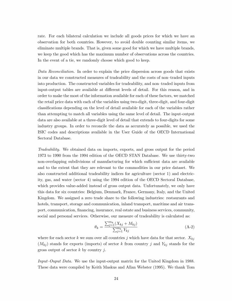
Tradeability. We obtained data on imports, exports, and gross output for the period

1973 to 1990 from the 1994 edition of the OECD STAN Database. We use thirty-two

non-overlapping subdivisions of manufacturing for which su¢cient data are available

and to the extent that they are relevant to the commodities in our price dataset. We

also constructed additional tradeability indices for agriculture (sector 1) and electric-

ity, gas, and water (sector 4) using the 1994 edition of the OECD Sectoral Database,

which provides value-added instead of gross output data. Unfortunately, we only have

this data for six countries: Belgium, Denmark, France, Germany, Italy, and the United

Kingdom. We assigned a zero trade share to the following industries: restaurants and

hotels, transport, storage and communication, inland transport, maritime and air trans-

port, communication, …nancing, insurance, real estate and business services, community,

social and personal services. Otherwise, our measure of tradeability is calculated as:

µk =

Pmkj=1(Xkj +Mkj)Pmk

j=1 Ykj(A-2)

where for each sector k we sum over all countries j which have data for that sector. Xkj(Mkj) stands for exports (imports) of sector k from country j and Ykj stands for the

gross output of sector k by country j.

Input–Ouput Data. We use the input-output matrix for the United Kingdom in 1988.

These data were compiled by Keith Maskus and Allan Webster (1995). We thank Tom

24

Prusa for suggesting this data source, which is available at the National Bureau of

Economic Research home page. Non–traded inputs are assumed to include: utilities,

construction, distribution, hotels, catering, railways, road transport, sea transport, air

transport, transport services, telecommunications, banking, …nance, insurance, business

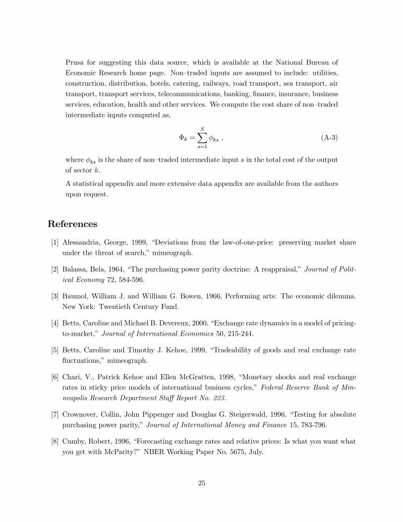
services, education, health and other services. We compute the cost share of non–traded

intermediate inputs computed as,

©k =SXs=1

Áks ; (A-3)

where Áks is the share of non–traded intermediate input s in the total cost of the output

of sector k.

A statistical appendix and more extensive data appendix are available from the authors

upon request.

References

[1] Alessandria, George, 1999, “Deviations from the law-of-one-price: preserving market share

under the threat of search,” mimeograph.

[2] Balassa, Bela, 1964, “The purchasing power parity doctrine: A reappraisal,” Journal of Polit-

ical Economy 72, 584-596.

[3] Baumol, William J. and William G. Bowen, 1966, Performing arts: The economic dilemma.

New York: Twentieth Century Fund.

[4] Betts, Caroline and Michael B. Devereux, 2000, “Exchange rate dynamics in a model of pricing-

to-market,” Journal of International Economics 50, 215-244.

[5] Betts, Caroline and Timothy J. Kehoe, 1999, “Tradeability of goods and real exchange rate

‡uctuations,” mimeograph.

[6] Chari, V., Patrick Kehoe and Ellen McGratten, 1998, “Monetary shocks and real exchange

rates in sticky price models of international business cycles,” Federal Reserve Bank of Min-

neapolis Research Department Sta¤ Report No. 223.

[7] Crownover, Collin, John Pippenger and Douglas G. Steigerwald, 1996, “Testing for absolute

purchasing power parity,” Journal of International Money and Finance 15, 783-796.

[8] Cumby, Robert, 1996, “Forecasting exchange rates and relative prices: Is what you want what

you get with McParity?” NBER Working Paper No. 5675, July.

25

[9] Ethier, Wilfred J., 1979, “Internationally decreasing costs and world trade,” Journal of Inter-

national Economics 9, 1-24.

[10] Engel, Charles, 1993, “Real exchange rates and relative prices: an empirical investigation,”

Journal of Monetary Economics 32, 35-50.

[11] Engel, Charles and John H. Rogers, 1996, “How wide is the border?” American Economic

Review 86, 1112-1125.

[12] Engel, Charles and John H. Rogers, 1999, “The welfare costs of deviations from the law of one

price: an empirical investigation,” mimeo.

[13] Eurostat, “Price structure of the Community countries,” Luxembourg: O¢ces of O¢cial Pub-

lications of the European Community, various issues.

[14] Feenstra, Robert C., 1995, “Estimating the e¤ects of trade policy,” in Gene M. Grossman

and Kenneth Rogo¤, eds., Handbook of International Economics, vol. 3. Amsterdam: North

Holland.

[15] Flam, Harry, 1992, “Product markets and 1992: full integration, large gains? Journal of

Economic Perspectives 6, 7-30.

[16] Froot, Kenneth A. Michael Kim and Kenneth Rogo¤, 1995, “The Law of One Price over 700

years,” National Bureau of Economic Research Working Paper No. 5132.

[17] Froot, Kenneth A. and Kenneth Rogo¤, 1995, “Perspectives on PPP and long-run real ex-

change rates,” in Gene M. Grossman and Kenneth Rogo¤, eds., Handbook of International

Economics, vol. 3. Amsterdam: North Holland.

[18] Ghosh Atish R. and Holger C. Wolf, 1994, “Pricing in international markets: lessons from the

Economist,” NBER Working Paper No. 4806, July.

[19] Giovannini, Alberto, 1988, “Exchange rates and traded goods prices,” Journal of International

Economics 24, 45-68.

[20] Haskel, Jonathan and Holger C. Wolf, 2000, “The law of one price - a case study,” mimeograph,

August.

[21] Isard, Peter, 1977, “How far can we push the Law of One Price,” American Economic Review

67(3), 942-948.

[22] Knetter, Michael M., 1989, “Price discrimination by U.S. and German exporters,” American

Economic Review 79, 198-210.

[23] Knetter, Michael M., 1993, “International comparisons of pricing-to-market behavior,” Amer-

ican Economic Review 83, 473-486.

26

[24] Kravis, Irving B. and Robert E. Lipsey, 1983, “Toward an explanation of national price levels,”

Princeton Studies in International Finance, No. 52, Princeton: Princeton University.

[25] Krugman, Paul R., 1987, “Pricing to market when the exchange rate changes,” in Real-…nancial

linkages among open economies Cambridge:MIT press, 49-70.

[26] Krugman, Paul R., 1995, “Increasing returns, imperfect competition and the positive the-

ory of international trade,” in Gene M. Grossman and Kenneth Rogo¤, eds., Handbook of

International Economics, vol. 3. Amsterdam: North Holland.

[27] Lutz, Mattias, 2001, “Pricing in segmented markets, arbitrage barriers and the law of one price:

evidence from the European car market,” University of St. Gallen, mimeograph, January.

[28] Maskus, Keith and Allan Webster, 1995, “Factor Specialization in U.S. and U.K. Trade: Sim-

ple Departures from the Factor-Content Theory,” Swiss Journal of Economics and Statistics,

1(131).

[29] Mussa, Michael, 1986, “Nominal exchange rate regimes and the behavior of real exchange

rates: Evidence and implications,” Carnegie-Rochester Series on Public Policy 25 (Autumn):

117-214.

[30] Obstfeld, Maurice and Kenneth Rogo¤, 2000, “The six major puzzles in international macroe-

conomics: is there a common cause?,” in Ben S. Bernanke and Kenneth Rogo¤, eds., NBER

Macroeconomics Annual 2000, Cambridge, MA: The MIT Press.

[31] Organization for Economic Co-operation and Development, 1995, STAN Database for Indus-

trial Analysis, computer diskettes, Paris: OECD.

[32] Parsley, David and Shang-Jin Wei, 2000, “Explaining the border e¤ect: the role of exchange

rate variability, shipping costs, and geography, NBER Working Paper No. 7836, August, forth-

coming, Journal of International Economics.

[33] Pigou, Arthur, 1920, “Some problems of foreign exchange,” Economic Journal 30, 460-472.

[34] Richardson, J. David, 1978, “Some empirical evidence on commodity arbitrage and the law of

on price,” Journal of International Economics 8, 341-351.

[35] Rogers, John H. and Michael Jenkins, 1995, “Haircuts or hysteresis? Sources of movements in

real exchange rates,” Journal of International Economics 38, 339-360.

[36] Rogers, John H., 2001, “Price level convergence, relative prices, and in‡ation in Europe,”Federal Reserve Board International Finance Discussion Paper, No. 699.

[37] Samuelson, Paul A., 1964, “Theoretical notes on trade problems,” Review of Economics and

Statistics 46, 145-154.

27

[38] Sanyal, Kalyan K. and Ronald W. Jones, 1982, “The theory of trade in middle products,”American Economic Review 72, 16-31.

[39] Sercu, Piet., Raman Uppal and C. Van Hulle, 1995, “The exchange rate in the presence of

transactions costs: implications for tests of purchasing power parity,” Journal of Finance 50,

1309-1319.

[40] Stockman, Alan C., and Linda L. Tesar, 1995, “Tastes and technology in a two-country model

of the business cycle,” American Economic Review 85, 168-185.

[41] Summers, Robert and Alan Heston, 1991, “The Penn World Table (Mark 5): An Expanded

Set of International Comparisons: 1950-1988,” Quarterly Journal of Economics 106, 327-368.

28

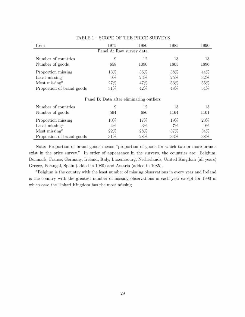
TABLE 1 – SCOPE OF THE PRICE SURVEYS

Item 1975 1980 1985 1990Panel A: Raw survey data

Number of countries 9 12 13 13Number of goods 658 1090 1805 1896

Proportion missing 13% 36% 38% 44%Least missinga 9% 23% 25% 32%Most missinga 27% 47% 53% 55%Proportion of brand goods 31% 42% 48% 54%

Panel B: Data after eliminating outliers

Number of countries 9 12 13 13Number of goods 594 686 1164 1101

Proportion missing 10% 17% 19% 23%Least missinga 4% 3% 7% 9%Most missinga 22% 28% 37% 34%Proportion of brand goods 31% 28% 33% 38%

Note: Proportion of brand goods means “proportion of goods for which two or more brands

exist in the price survey.” In order of appearance in the surveys, the countries are: Belgium,

Denmark, France, Germany, Ireland, Italy, Luxembourg, Netherlands, United Kingdom (all years)

Greece, Portugal, Spain (added in 1980) and Austria (added in 1985).aBelgium is the country with the least number of missing observations in every year and Ireland

is the country with the greatest number of missing observations in each year except for 1990 in

which case the United Kingdom has the most missing.

29

30

TABLE 3 – TRADE SHARES

Industry Trade shareAgriculture, hunting, forestry and …shing 0.403Food 0.281Beverages 0.266Tobacco 0.171Textiles 0.576Wearing apparel 0.552Leather products 0.667Footwear 0.634Furniture and …xtures 0.254Paper and paper products 0.494Printing and publishing 0.151Industrial chemicals 0.806Other chemicals 0.468Chemical products, n.e.c. 0.498Misc. products of petroleum and coal 0.416Rubber products 0.533Plastic products, n.e.c. 0.272Pottery, china etc. 0.261Non-metal products, n.e.c. 0.200Iron and steel 0.450Non-ferrous metals 0.682Fabricated metal products, except machinery and equipment 0.354O¢ce and computing machinery 1.280Machinery and equipment, n.e.c. 0.586Electrical machinery 0.486Radio, television and communication equipment 0.588Electrical apparatus, n.e.c. 0.467Shipbuilding and repairing 0.431Motor vehicles 0.618Motorcycles and bicycles 0.635Professional goods 1.295Other manufacturing n.e.c. 1.276Electricity, gas and steam and water 0.856

Source: OECD Sectoral Database and OECD STAN Database.

Note: The following industries have been assigned a zero trade share: restaurants and

hotels, transport, storage and communication, inland transport, maritime and air trans-

port, communication, …nancing, insurance, real estate and business services, community,

social and personal services.

31

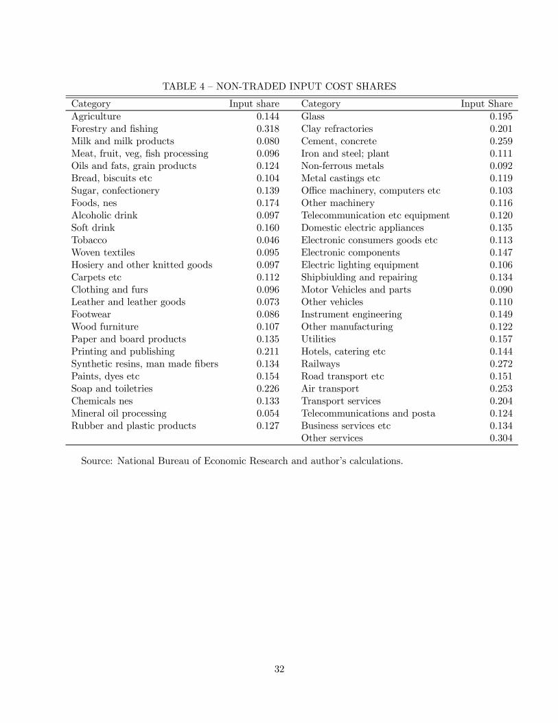
TABLE 4 – NON-TRADED INPUT COST SHARES

Category Input share Category Input ShareAgriculture 0.144 Glass 0.195Forestry and …shing 0.318 Clay refractories 0.201Milk and milk products 0.080 Cement, concrete 0.259Meat, fruit, veg, …sh processing 0.096 Iron and steel; plant 0.111Oils and fats, grain products 0.124 Non-ferrous metals 0.092Bread, biscuits etc 0.104 Metal castings etc 0.119Sugar, confectionery 0.139 O¢ce machinery, computers etc 0.103Foods, nes 0.174 Other machinery 0.116Alcoholic drink 0.097 Telecommunication etc equipment 0.120Soft drink 0.160 Domestic electric appliances 0.135Tobacco 0.046 Electronic consumers goods etc 0.113Woven textiles 0.095 Electronic components 0.147Hosiery and other knitted goods 0.097 Electric lighting equipment 0.106Carpets etc 0.112 Shipbiulding and repairing 0.134Clothing and furs 0.096 Motor Vehicles and parts 0.090Leather and leather goods 0.073 Other vehicles 0.110Footwear 0.086 Instrument engineering 0.149Wood furniture 0.107 Other manufacturing 0.122Paper and board products 0.135 Utilities 0.157Printing and publishing 0.211 Hotels, catering etc 0.144Synthetic resins, man made …bers 0.134 Railways 0.272Paints, dyes etc 0.154 Road transport etc 0.151Soap and toiletries 0.226 Air transport 0.253Chemicals nes 0.133 Transport services 0.204Mineral oil processing 0.054 Telecommunications and posta 0.124Rubber and plastic products 0.127 Business services etc 0.134

Other services 0.304

Source: National Bureau of Economic Research and author’s calculations.

32

TABLE 5 –LOG REAL EXCHANGE RATES

Consumption expenditureGNP Equally weighted share weighted

Countrya (1990 $) 1975 1980 1985 1990 1975 1980 1985 1990Luxembourg 16,399 -0.051 -0.019 -0.092 -0.074 -0.112 -0.097 -0.128 -0.116(1957) (0.011) (0.010) (0.011) (0.012)

Germany 14,478 0.020 0.043 -0.048 -0.004 0.012 0.017 -0.025 0.010(1957) (0.014) (0.016) (0.013) (0.014)

France 13,931 0.077 0.067 -0.001 0.015 0.114 0.076 0.047 0.019(1957) (0.012) (0.014) (0.014) (0.015)

Denmark 13,802 0.140 0.176 0.166 0.163 0.181 0.201 0.195 0.234(1957) (0.017) (0.018) (0.018) (0.019)

United Kingdom 13,066 -0.240 0.010 -0.062 -0.087 -0.209 0.053 0.012 -0.032(1973) (0.019) (0.019) (0.016) (0.021)

Netherlands 12,858 -0.025 -0.019 -0.109 -0.057 -0.035 0.007 -0.080 -0.029(1957) (0.012) (0.014) (0.014) (0.014)

Austria 12,849 0.029 0.020 0.050 0.072(1995) (0.015) (0.017)

Italy 12,555 -0.094 -0.128 -0.077 -0.035 -0.126 -0.137 -0.080 0.009(1957) (0.019) (0.019) (0.019) (0.018)

Spain 11,020 -0.152 -0.165 -0.129 -0.212 -0.193 -0.124(1986) (0.021) (0.019) (0.019)

Ireland 9,067 -0.239 -0.074 -0.025 -0.040 -0.303 -0.074 0.025 0.027(1973) (0.020) (0.020) (0.019) (0.018)

Greece 6,678 -0.208 -0.253 -0.237 -0.258 -0.289 -0.138(1981) (0.025) (0.022) (0.023)

Portugal 6,520 -0.280 -0.264 -0.320 -0.408 -0.403 -0.332(1986) (0.029) (0.024) (0.024)

Note: Entries in columns 3 to 10 are qj , the weighted average for country j of good-speci…c log

relative prices. For these calculations we eliminate multiple brands of the same good. The numbers

in parentheses are standard errors of the equally-weighted means.a The year the country joined the European Union is in parentheses. Strictly speaking the

term European Union subsumes the history of various forms of institutional arrangements. The

European Economic Community (EEC) was formally established by one of the Treaties of Rome

in 1957 and the European Community was established in 1967 as the merger of the EEC, the

European Coal and Steel Community and the European Atomic Energy Community.

33

34

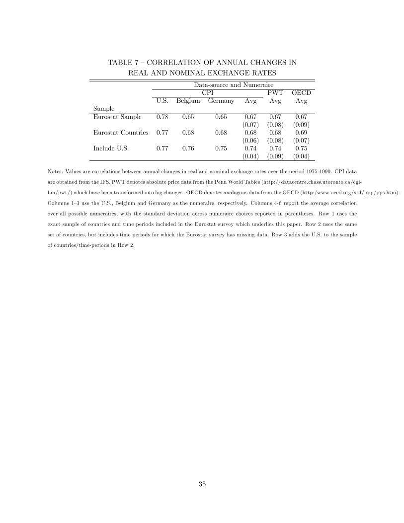
TABLE 7 – CORRELATION OF ANNUAL CHANGES IN

REAL AND NOMINAL EXCHANGE RATES

Data-source and NumeraireCPI PWT OECD

U.S. Belgium Germany Avg Avg AvgSampleEurostat Sample 0.78 0.65 0.65 0.67 0.67 0.67

(0.07) (0.08) (0.09)Eurostat Countries 0.77 0.68 0.68 0.68 0.68 0.69

(0.06) (0.08) (0.07)Include U.S. 0.77 0.76 0.75 0.74 0.74 0.75

(0.04) (0.09) (0.04)

Notes: Values are correlations between annual changes in real and nominal exchange rates over the period 1975-1990. CPI data

are obtained from the IFS. PWT denotes absolute price data from the Penn World Tables (http://datacentre.chass.utoronto.ca/cgi-

bin/pwt/) which have been transformed into log changes. OECD denotes analogous data from the OECD (http:/www.oecd.org/std/ppp/pps.htm).

Columns 1–3 use the U.S., Belgium and Germany as the numeraire, respectively. Columns 4-6 report the average correlation

over all possible numeraires, with the standard deviation across numeraire choices reported in parentheses. Row 1 uses the

exact sample of countries and time periods included in the Eurostat survey which underlies this paper. Row 2 uses the same

set of countries, but includes time periods for which the Eurostat survey has missing data. Row 3 adds the U.S. to the sample

of countries/time-periods in Row 2.

35

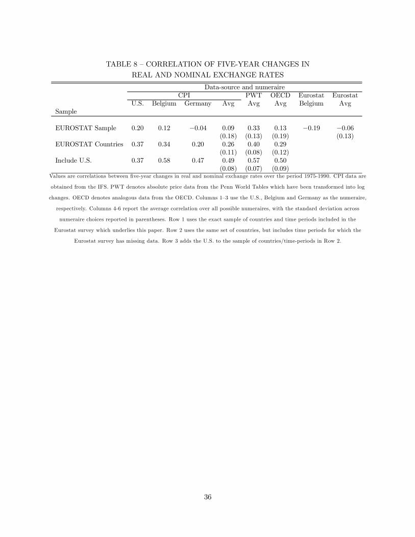
TABLE 8 – CORRELATION OF FIVE-YEAR CHANGES IN

REAL AND NOMINAL EXCHANGE RATES

Data-source and numeraireCPI PWT OECD Eurostat Eurostat

U.S. Belgium Germany Avg Avg Avg Belgium AvgSample

EUROSTAT Sample 0.20 0.12 ¡0.04 0.09 0.33 0.13 ¡0.19 ¡0.06(0.18) (0.13) (0.19) (0.13)

EUROSTAT Countries 0.37 0.34 0.20 0.26 0.40 0.29(0.11) (0.08) (0.12)

Include U.S. 0.37 0.58 0.47 0.49 0.57 0.50(0.08) (0.07) (0.09)

Values are correlations between …ve-year changes in real and nominal exchange rates over the period 1975-1990. CPI data are

obtained from the IFS. PWT denotes absolute price data from the Penn World Tables which have been transformed into log

changes. OECD denotes analogous data from the OECD. Columns 1–3 use the U.S., Belgium and Germany as the numeraire,

respectively. Columns 4-6 report the average correlation over all possible numeraires, with the standard deviation across

numeraire choices reported in parentheses. Row 1 uses the exact sample of countries and time periods included in the

Eurostat survey which underlies this paper. Row 2 uses the same set of countries, but includes time periods for which the

Eurostat survey has missing data. Row 3 adds the U.S. to the sample of countries/time-periods in Row 2.

36

TABLE 9 – COUNTRY EFFECTS

Country 1975 1980 1985 1990Austria n.a. n.a. 0.077 0.070

n.a. n.a. (0.008) (0.010)

Belgium 0.020 0.002 0.025 -0.003(0.007) (0.009) (0.009) (0.008)

Denmark 0.189 0.240 0.251 0.267(0.013) (0.015) (0.012) (0.015)

France 0.109 0.073 0.043 0.037(0.009) (0.011) (0.009) (0.009)

Germany 0.039 0.055 -0.024 0.009(0.010) (0.012) (0.008) (0.008)

Greece n.a. -0.090 -0.083 -0.073n.a. (0.017) (0.014) (0.014)

Ireland -0.167 -0.029 0.043 0.018(0.012 (0.013) (0.013) (0.012)

Italy -0.034 -0.086 -0.004 0.012(0.012) (0.012) (0.011) (0.011)

Luxembourg -0.027 -0.020 -0.085 -0.072(0.007) (0.009) (0.007) (0.007)

Netherlands 0.007 0.000 -0.066 -0.026(0.008) (0.010) (0.008) (0.008)

Portugal n.a. -0.132 -0.102 -0.160n.a. (0.019) (0.016) (0.012)

Spain n.a. -0.057 -0.065 -0.043n.a. (0.013) (0.011) (0.010)

United Kingdom -0.167 0.020 0.001 -0.025(0.011) (0.013) (0.011) (0.014)

Percent Explained 20.90 10.13 9.13 11.53Percent Unexplained 82.60 91.46 93.10 92.17Residual -3.49 -1.59 -2.23 -3.70

Note: Entries represent the average, across goods for a particular country, of the percent by

which each price deviates from its good-speci…c mean. Speci…cally, given the price of the ith good

in the jth country, and the nominal exchange rate, ej, the means are calculated as

Mean =1

Nj

NjXi

ÃejpijPMi

j=1 ejpij=Mi

¡ 1!:

The residual associated with the variance decomposition is due to missing observations or, equiva-

lently, an unequal number of observations, Nj, for each country, j.

37

TABLE 10 – PRICE DISPERSION SUMMARY STATISTICS

1975 1980 1985 1990Overall price dispersion 0.188 0.236 0.242 0.229

Dispersion by characteristic:

Non-traded 0.253 0.321 0.329 0.325Traded 0.178 0.223 0.229 0.214

Above average share of services 0.214 0.287 0.292 0.306Below average share of services 0.183 0.228 0.234 0.219

Branded goods 0.153 0.211 0.201 0.191Non-branded goods 0.204 0.246 0.262 0.252

Notes: Authors calculations.

38

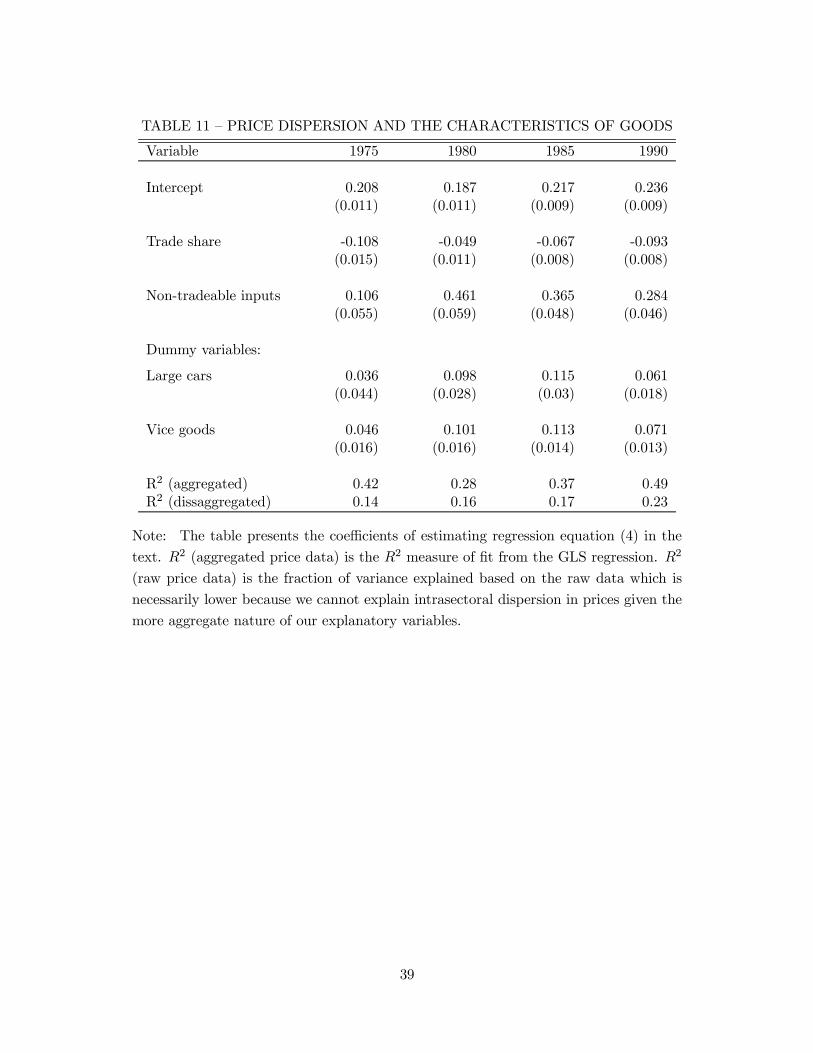
TABLE 11 – PRICE DISPERSION AND THE CHARACTERISTICS OF GOODS

Variable 1975 1980 1985 1990

Intercept 0.208 0.187 0.217 0.236(0.011) (0.011) (0.009) (0.009)

Trade share -0.108 -0.049 -0.067 -0.093(0.015) (0.011) (0.008) (0.008)

Non-tradeable inputs 0.106 0.461 0.365 0.284(0.055) (0.059) (0.048) (0.046)

Dummy variables:

Large cars 0.036 0.098 0.115 0.061(0.044) (0.028) (0.03) (0.018)

Vice goods 0.046 0.101 0.113 0.071(0.016) (0.016) (0.014) (0.013)

R2 (aggregated) 0.42 0.28 0.37 0.49R2 (dissaggregated) 0.14 0.16 0.17 0.23

Note: The table presents the coe¢cients of estimating regression equation (4) in the

text. R2 (aggregated price data) is the R2 measure of …t from the GLS regression. R2

(raw price data) is the fraction of variance explained based on the raw data which is

necessarily lower because we cannot explain intrasectoral dispersion in prices given the

more aggregate nature of our explanatory variables.

39

40

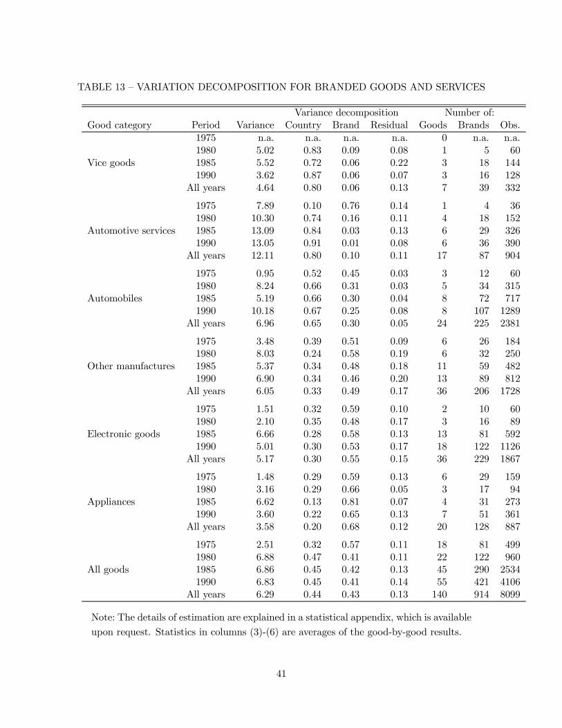
TABLE 13 – VARIATION DECOMPOSITION FOR BRANDED GOODS AND SERVICES

Variance decomposition Number of:Good category Period Variance Country Brand Residual Goods Brands Obs.

1975 n.a. n.a. n.a. n.a. 0 n.a. n.a.1980 5.02 0.83 0.09 0.08 1 5 60

Vice goods 1985 5.52 0.72 0.06 0.22 3 18 1441990 3.62 0.87 0.06 0.07 3 16 128

All years 4.64 0.80 0.06 0.13 7 39 332

1975 7.89 0.10 0.76 0.14 1 4 361980 10.30 0.74 0.16 0.11 4 18 152

Automotive services 1985 13.09 0.84 0.03 0.13 6 29 3261990 13.05 0.91 0.01 0.08 6 36 390

All years 12.11 0.80 0.10 0.11 17 87 904

1975 0.95 0.52 0.45 0.03 3 12 601980 8.24 0.66 0.31 0.03 5 34 315

Automobiles 1985 5.19 0.66 0.30 0.04 8 72 7171990 10.18 0.67 0.25 0.08 8 107 1289

All years 6.96 0.65 0.30 0.05 24 225 2381

1975 3.48 0.39 0.51 0.09 6 26 1841980 8.03 0.24 0.58 0.19 6 32 250

Other manufactures 1985 5.37 0.34 0.48 0.18 11 59 4821990 6.90 0.34 0.46 0.20 13 89 812

All years 6.05 0.33 0.49 0.17 36 206 1728

1975 1.51 0.32 0.59 0.10 2 10 601980 2.10 0.35 0.48 0.17 3 16 89

Electronic goods 1985 6.66 0.28 0.58 0.13 13 81 5921990 5.01 0.30 0.53 0.17 18 122 1126

All years 5.17 0.30 0.55 0.15 36 229 1867

1975 1.48 0.29 0.59 0.13 6 29 1591980 3.16 0.29 0.66 0.05 3 17 94

Appliances 1985 6.62 0.13 0.81 0.07 4 31 2731990 3.60 0.22 0.65 0.13 7 51 361

All years 3.58 0.20 0.68 0.12 20 128 887

1975 2.51 0.32 0.57 0.11 18 81 4991980 6.88 0.47 0.41 0.11 22 122 960

All goods 1985 6.86 0.45 0.42 0.13 45 290 25341990 6.83 0.45 0.41 0.14 55 421 4106

All years 6.29 0.44 0.43 0.13 140 914 8099

Note: The details of estimation are explained in a statistical appendix, which is available

upon request. Statistics in columns (3)-(6) are averages of the good-by-good results.

41

-2 0 20

0.01

0.02

0.03

0.04Denmark

-2 0 20

0.01

0.02

0.03

0.04France

-2 0 20

0.01

0.02

0.03

0.04Germany

-2 0 20

0.01

0.02

0.03

0.04Ireland

-2 0 20

0.01

0.02

0.03

0.04Italy

-2 0 20

0.01

0.02

0.03

0.04Luxembourg

-2 0 20

0.01

0.02

0.03

0.04Netherlands

-2 0 20

0.01

0.02

0.03United Kingdom

-2 0 20

0.01

0.02

0.03

0.04Pooled

Figure 1: Empirical distributions of law-of-one-price deviations

Each line represents an estimate of the density of good-by-good deviations from the Law-of-One-

Price between Belgium (the numeraire) and some other EC country. More speci…cally, each line is

an estimate of the density, for country j, of qij = log(ejpij=pin), where pij is the price of good i

in country j, denominated in domestic currency and ej is the spot exchange rate between country

j and Belgium. Each chart contains a bilateral comparison between Belgium and one other EC

country for each year in our panel. We present the individual country densities only for those

countries with 4 years of available data. However, the lower right-hand chart presents an estimated

density for each year (1975, 1980, 1985 and 1990), pooled across all countries with data available

for the year under examination.

42

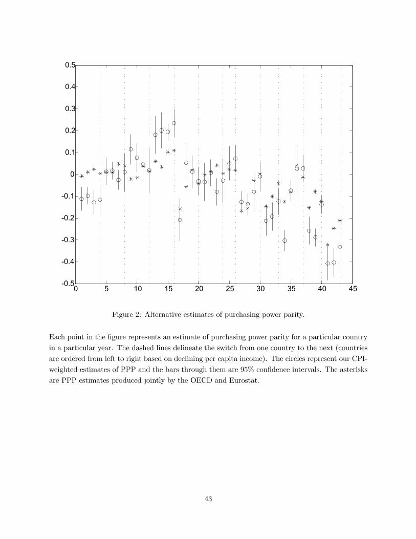
0 5 10 15 20 25 30 35 40 45-0.5

-0.4

-0.3

-0.2

-0.1

0

0.1

0.2

0.3

0.4

0.5

Figure 2: Alternative estimates of purchasing power parity.

Each point in the …gure represents an estimate of purchasing power parity for a particular country

in a particular year. The dashed lines delineate the switch from one country to the next (countries

are ordered from left to right based on declining per capita income). The circles represent our CPI-

weighted estimates of PPP and the bars through them are 95% con…dence intervals. The asterisks

are PPP estimates produced jointly by the OECD and Eurostat.

43

0 0.1 0.2 0.3 0.4 0.5 0.60

0.005

0.01

0.015

0.02

0.025

0.03 19751980

1985, 1990

Figure 3: Empirical distributions of good-by-good cross-country price dispersion.

Each line represents an estimate of the density of the mean absolute deviation of national prices

compared to the cross-country mean, good-by-good, for a particular year in the cross-section.

Speci…cally, the dispersion measure is de…ned as: yi = mad(zij), where zij =ejpijPMi

j=1 ejpij=Mi

¡ 1.

44