understanding and using time series analyses in addiction
TRANSCRIPT

This article has been accepted for publication and undergone full peer review but has not been through the copyediting, typesetting, pagination and proofreading process which may lead to differences between this version and the Version of Record. Please cite this article as doi: 10.1111/add.14643
This article is protected by copyright. All rights reserved.
Beard Emma (Orcid ID: 0000-0001-8586-1261)
Marsden John (Orcid ID: 0000-0002-1307-2498)
Brown Jamie (Orcid ID: 0000-0002-2797-5428)
Understanding and using time series analyses in addiction research
Emma Beard 1, 2, John Marsden 3, Jamie Brown 1,2, Ildiko Tombor 2, John Stapleton 1,3, Susan Michie
1, Robert West 2
1 Research Department of Clinical, Educational and Health Psychology, University College London,
London
2 Department of Behavioural Science and Health, University College London, London
3 Addictions Department, Institute of Psychiatry, Psychology and Neuroscience, King’s College
London, United Kingdom;
Abstract: 181 words
Main text: 7114 words
Suggested running head: Time series analysis in addiction research
Keywords: time series, ARIMA, ARIMAX, VAR, SVAR, VECM, addiction
___________

This article is protected by copyright. All rights reserved.
* Corresponding author: Emma Beard, Senior Research Associate, Research Department of Clinical,
Educational and Health Psychology, University College London, London; e-mail address:
ABSTRACT
Time series analyses are statistical methods used to assess trends in repeated measurements taken
at regular intervals and their associations with other trends or events taking account of the
temporal structure of such data. Addiction research often involves assessing associations between
trends in target variables (e.g. population cigarette smoking prevalence) and predictor variables
(e.g. average price of a cigarette) known as a multiple time series design, or interventions or events
(e.g. introduction of an indoor smoking ban) known as an interrupted time series design. There are
many analytical tools available, each with its own strengths and limitations. This paper provides
addiction researchers with an overview of many of the methods available (GLM, GLMM, GLS,
GAMM, ARIMA, ARIMAX, VAR, SVAR, VECM), and guidance on when and how they should be used,
sample size determination, reporting, and interpretation. The aim is to provide increased clarity for
researchers proposing to undertake these analyses concerning what is likely to be acceptable for
publication in journals such as Addiction. Given the large number of choices that need to be made
when setting up time series models, the guidance emphasises the importance of pre-registering
hypotheses and analysis plans before the analyses are undertaken.
This article is protected by copyright. All rights reserved.
INTRODUCTION
Time series analyses (TSA) are statistical methods for the analysis of multiple measurements of one
or more variables over time. Sometimes these data reflect responses collected from a single
research participant; but more commonly in social, behavioural and epidemiological research, TSA
are used to study a variable of interest aggregated for a group, region or country. TSA can be a
powerful tool for informing public health policy. There are comprehensive modules on TSA in
statistical software (e.g. R and STATA) and several textbooks (1-4). TSA require the researcher to
navigate a process of statistical modelling that requires a grasp of concepts, terminology and
parameters that will be new to many in the addiction sciences.
This article provides an introduction to the topic, tailored to addiction research, setting out when it
is appropriate to use each method and how to report and interpret findings. The paper is
structured in four parts: Part 1 covers uses of TSA and how to plan the analyses; Part 2 focuses on
TSA concepts and requirements; Part 3 looks at how to conduct TSA; and Part 4 describes how to
report the results. For space reasons, we limit the article to the main TSA approaches that are
supported by major statistical packages. The main types of analysis covered are: Generalised Least-
Squares (GLS) and Generalised Linear Mixed Models (GLMM), Generalised Additive Mixed Models
(GAMM), Autoregressive Integrated Moving Average (ARIMA) and Autoregressive Integrated
Moving Average with Exogenous Variables (ARIMAX) models, Vector Autoregression (VAR) and
Structural Vector Autoregressive models (SVAR), and Vector Error Correction Models (VECM).
PART 1: USES OF TSA AND PLANNING THE ANALYSES
Uses of TSA
There are several types of question that can be addressed by TSA. Simple ‘trend analysis’ assesses
whether there is evidence for a change in the level of a series over time. For example, a study of
first year college students used TSA to assess whether there was an increase in use of tobacco,
alcohol and cannabis at the beginning and end of the academic year (5).
‘Multiple TSA’ assess whether a temporal trend in a target variable is linked to trends in other
variables. In the smoking field, Beard et al examined whether the growth in prevalence of e-
cigarette use was linked to a decline in the use of licensed nicotine products such as nicotine skin
patches (6). Langley et al assess the temporal association between a standardised measure of
tobacco control advertising exposure on television and the number of calls to a national stop

This article is protected by copyright. All rights reserved.
smoking helpline (7). Brunt et al assess the association between changes in the price and quality of
cocaine and changes in the incidence of addiction treatment episodes and hospital admissions (8).
‘Interrupted TSA’ assess whether an event or shift in policy was associated with a change in the
trend of a target variable. For example, Holder and Wagenaar studied changes in the rate of road
traffic crashes after the introduction of a law on training for responsible alcohol-serving in licensed
premises (9). An interrupted TSA was used to evaluate the effect on smoking prevalence of the
partial tobacco point of sale display ban in large shops in England (10). Other studies have used
interrupted TSA to evaluate: the impact on smoking cessation of temporarily suspending large-scale
tobacco mass media campaigns (11); the introduction of the smoking cessation drug, varenicline,
on prescribing of smoking cessation medications (12); the impact of introducing flexible alcohol
trading hours on rates of violence, robbery and total crime (13); and changes in sale of alcohol
following a ban on discounted alcohol products in shops and supermarkets (14).
TSA are also used in ‘forecasting’: projecting forward from past values of a series. For example,
alcohol consumption over a prospective 10-year period was forecast for the Czech Republic (15). In
the United States, age-specific mortality rates for men and women have been forecast using the
decline in the prevalence of tobacco smoking (16).
Data sources and design issues
There are many suitable data sources for TSA, including official registries, repeated cross-sectional
surveys and longitudinal studies of cohorts and panels. Examples include the Swiss HIV Cohort
Study established in 1988 which continuously enrolled HIV-infected people who attended out-
patient clinics at seven centres (17), and The Health Improvement Network (THIN) database in
England (18, 19). TSA can be difficult to use in cohort and panel samples because of follow-up
attrition (20), but this situation is improving with the advent of mobile/smartphone technologies
(21-23).
At an individual level, data can be used from multiple repeated measurements from individuals in
n-of-1 studies. For example, ecological momentary assessment generates large quantities of data
from individuals (24) and digital mobile applications similarly can generate time series on usage,
inputs, processes and outcomes (25).
In multiple TSA the coefficient linking a given input series to an output series can be interpreted as
the association between the input and output series after adjusting for or removing any underlying
trend and other input series included in the analysis. In interrupted TSA, a ‘dummy’ variable (taking

This article is protected by copyright. All rights reserved.
the value 0 or 1) is used in the input series to reflect time points when events occur, or pre-versus
post-initiation of a policy etc. The resulting coefficient can be interpreted as the change in the value
or trend of the outcome variable linked to the presence or onset of the event or policy after
adjusting for or removing any underlying trend and other input variables (11). TSA can be used
with many types of data, including counts and percentages (e.g. number of heroin users arrested,
the number of fatal drug-related poisoning cases, and the prevalence of adult smoking), binary data
and continuous measures (e.g. amount spent on alcohol per week).
It is important to appreciate limitations of TSA. First, they can only assess associations at the
temporal granularity of the series. Thus if the data are weekly, TSA are assessing week-by-week
changes, not changes over a longer or shorter time frame. For example, showing an association
between monthly spend on anti-tobacco mass media campaigns and attempts to stop smoking
does not mean that a similar association would be found with annual spend. Secondly, TSA have
limited ability to detect associations between input and output variables that accumulate over a
long period. For example, anti-alcohol mass media campaigns may not have a detectable effect in
the short term but may contribute to cultural change that accumulates over a period of years.
Detecting such an effect would be very problematic for TSA.
Sample size
Statistical power calculations can inform study planning (26). Unfortunately, power calculations,
such as those provided for linear regression and ANOVA in G*Power(27, 28), are not suitable for
time series data. In TSA it is necessary to account for autocorrelation, seasonality and lag effects
(see below). Calculations are provided by McLeod and Vingili (29, 30) for interrupted time series
designs. However, the recommended method is to use a power simulation, and there are several
statistical packages that can do this (e.g. R). The procedure involves running many TSA models on
randomly generated data with expected parameter estimates and calculating power from the
proportion of observations which return results at a given level of statistical significance.
In general, the sample size required will increase with the number of parameters to be estimated,
and the amount of noise in the data. It is important to accurately reflect changes over time in the
simulation and to include all covariate estimates of interest. There should always be more time
points than the total number of variables, autocorrelation and lag terms and some experts
recommend at least 50-100 time points (31-33). At least two years of monthly data has been
proposed to allow adjustment for seasonality, with a preference for equal proportions of data
collection before and after the event or change in the input variable for an interrupted TSA (26).

This article is protected by copyright. All rights reserved.
Individual-level analyses generally provide greater power, and a larger number of observations
aggregated to create each data point are likely to give more stable estimates (34).
PART 2: TIME SERIES CONCEPTS
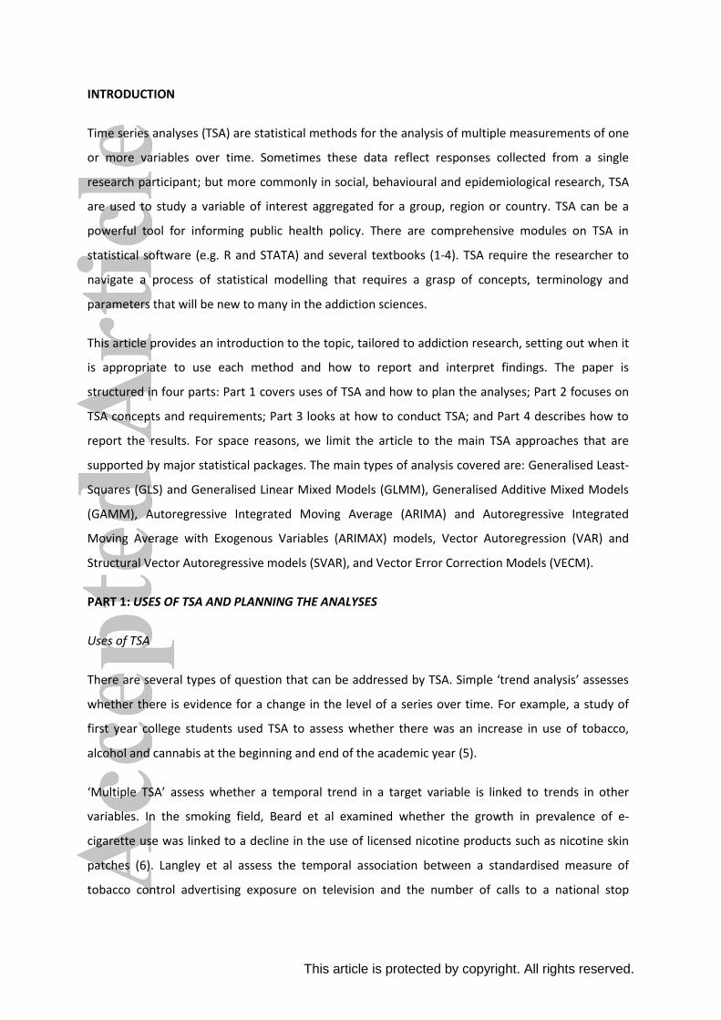
The data for any TSA are typically partitioned into three main components: a trend component, a
seasonal component and a random component (35). As an example, Figure 1 displays a
hypothetical de-composition of data on the prevalence of excessive alcohol consumption over time
(36 monthly waves of data collection).
The ‘trend’ chart in the top right-hand panel shows a plotted trend derived from observed data in
the top left panel (using a 12-month two-point moving average). It appears that the prevalence
declines in a roughly linear manner over time.
The ‘seasonal’ chart in the bottom left panel in Figure 1 shows a cyclical pattern derived from the
data in the top left panel. We note that weekly seasonality can be modelled if the data are
collected daily. This would reflect cyclical changes due to the day of the week (e.g. showing that
more alcohol is consumed at the weekend).
The ‘random’ chart shows the component that represents unexplained variance. This represents
any remaining variation in the series that is not accounted for by the trend and seasonality
components.
Underlying trends and stationarity
To make inferences about the impact of the introduction of a policy or intervention or how two
time series covary it is important to address any underlying long-term trends. This can be done
either a) by systematically modelling the trend or b) removing it from the data. Screening a data
series for an underlying trend is achieved by assessing the association between values and their
position in the series.
Modelling of the underlying trend in a series can be accomplished by including a linear or
polynomial term reflecting time points as an independent variable in a statistical model. Greater
flexibility can be achieved with the use of fractional polynomials or what are known as ‘restricted
cubic splines’.
Removing any underlying trend involves transforming the data in some way to make it ‘stationary’
(stationary refers to a time series is one whose statistical properties such as mean, variance,

This article is protected by copyright. All rights reserved.
autocorrelation, etc. are all constant over time).. There are several options for making a series
stationary. First, one can remove a trend through ‘differencing’, which involves using the
differences between observations rather than the observations themselves. A series of ‘first
differences’ (subtract values at time t from values at time t+1) will work to remove linear trends
(36). ‘Seasonal differencing’ involves subtracting values from values that are a fixed number of time
points ahead (e.g. taking values at t from values at t+12 in monthly data).
In situations where there is evidence of a non-constant slope (e.g. an exponential trend), second
differences (taking the first difference of the already differenced series) will often render the series
stationary (37) In practice, it is almost never necessary to go beyond second differencing (36).
However, if a series does exhibit higher degree polynomial trends, an order of differencing equal to
that degree may be required (38).
There are several ‘unit root’ tests that can help determine the number of differences required for
the time series to be made stationary. Two of the most commonly used of these are the augmented
Dickey-Fuller (ADF) test and the Phillips Perron tests (39, 40).
Researchers should guard against over-differencing. To assess the presence of over-differencing,
the autocorrelation of the differenced data should be calculated (see below). A rule of thumb is
that the lag-1 autocorrelation should not be more negative than -0.5 (see section on
autocorrelation for more details) (41).
Another way to address non-stationarity is to use natural logarithmic or square root
transformations (38). Of the two, the natural logarithmic transformation is often preferred as it has
the statistical property of converting absolute changes to percentage changes, which makes for
easier interpretation of the outputs. The main priority here is to stabilise the variance of the
underlying series. Failure to stabilise the variance can reduce forecasting precision and undermine
accurate assessment of associations (42). It is often necessary to difference and transform a time
series.
In the previous example of prevalence of excessive alcohol consumption, the ADF test suggested
that one order of differencing was required with no seasonal differencing. Figure 2 shows a plot of
the time series data for excessive alcohol consumption following a natural log transformation and
first order differencing.
Autocorrelation

This article is protected by copyright. All rights reserved.
There is autocorrelation within a series if values in the series are in some way statistically
associated with earlier values. There are two main types of autocorrelation: autoregressive (AR)
and moving average (MA). The former occurs when values in a series are correlated with earlier
values. The latter occurs when values in a series are a function of the degree of prediction error of
earlier values after taking account of any correlation between the values. For example, AR(1) means
that values of a series at one point in time are correlated with immediately preceding values. MA(1)
means that values of a series are a function of the difference between the immediately preceding
value and a predicted value (the error) from a regression of values on to immediately preceding
values. In both cases the ‘lag’ is said to be one. Where the autocorrelations involve preceding
values going further back from the current values, the lag value increases.
The degree of autocorrelation across a set of lags is called the autocorrelation function (ACF) and
this plays a key role in model selection and evaluation. To determine which type of autocorrelation
applies in a given case, the researcher checks the ACF and Partial ACF (PACF). The PACF shows
autocorrelations between values at a point in time and the lagged values 1, 2, 3 etc in which
correlations for higher lags are adjusted for correlations at lower lags.
As a rule of thumb, if the PACF displays a sharp cut-off (for example a large lag-1 autocorrelation
but small lag autocorrelation and/or the lag-1 autocorrelation is positive), it is best to add an AR
term. If the ACF displays a sharp cut-off and/or the lag-1 autocorrelation is negative, the addition of
an MA term should be considered (43). For example, the ACF and PACF in Figure 3 suggest an MA
and AR autocorrelation term may be needed, as both cut off abruptly after a lag of 1 and 2
respectively.
Lagged effects
The effects of an intervention or event can be gradual or delayed. In these cases, lagged effects
need to be considered in the analysis (34). For example, a hypothetical intervention may have been
introduced in July 2008 but publicity campaigns were not implemented until two months later. In
this instance one would model the impact of the intervention in July 2008 and the impact of the
intervention assuming a delay in August 2008 and September 2008. Alternative models with varying
lag effects can be compared using a measure of fit such as the Bayesian Information Criterion (BIC)
or Akaike's Information Criterion (AIC(43)).
Lagged effects can also be encountered in multiple TSA. For example, monthly prevalence of
smoking cessation may not immediately impact on alcohol consumption but may start to have an
effect a month or two later (44). The presence of lags can be assessed using the same methods as
This article is protected by copyright. All rights reserved.
for interrupted TSA or by using the sample cross correlation function (CCF). The CCF provides a set
of sample correlations between the input series (X) at time t+h and the output series (Y) at time t,
where h can be any value reflecting past or future points of data collection. For example, the
researcher may be interested in the effect on the output series (Y) at month three of the input
series (X) two months prior i.e., 𝑋3−2~𝑌3 (3).
Generally, ‘pre-whitened’ data are used in conjunction with the CCF as this aids interpretation by
removing autocorrelation in the series that may cause spurious cross-correlation effects. Pre-
whitening decorrelates the input series and then applies the same filter (autoregressive model) to
the output series.
Confounding
Causality can generally be inferred from randomised controlled trials (i.e. where participants are
randomly assigned to an intervention versus comparison group) and procedures are put in place to
remove bias, such as blinding participants. Although causality can less confidently be inferred from
observational research designs, an assessment can be done to determine how far causal inference
is justified (e.g. using the Bradford Hill Criteria (45)). Whether the design is experimental or
observational, it is important to consider, measure and adjust for potential confounding in TSA. At
the individual level this may involve including socio-demographic characteristics; at the population
level it may involve other interventions and policies that are being introduced in that population.
These potential confounders should be pre-defined in the analysis plan.
Outliers
Outliers are values that are very different from the majority of those in a time series. Outliers can
be problematic for TSA because they may exert a disproportionate influence on coefficient
estimates (46). Outliers may be justifiably removed if they are determined to be errors and they fall
at the start or end of the series.
One useful package is ‘tsoutliers’ in R which identifies and suggests possible replacement values by
using an iterative outlier detection approach descibed by Chen and Liu (47, 48). However, this
procedure may misidentify a valid shift in level as an outlier or fail to detect outliers due to masking
(49). If outliers are removed it is important to run and report a sensitivity analysis with their
inclusion (50). The procedure for detecting and removing outliers should be pre-specified in the
statistical analysis plan to reduce risk of researcher bias.

This article is protected by copyright. All rights reserved.
Missing data
Missing data present major problems for TSA. If TSA are being conducted on aggregated data from
surveys or cohorts and these have differing amounts and types of missing data in the samples
generating the aggregate value, any temporal changes may reflect this ‘missingness’ rather than
anything real in the population.
If data for particular time points are completely missing, TSA cannot be undertaken unless
assumptions are made to impute those missing values. ‘Last observation carried forward’ or ‘mean
subtitution’ are sometimes used but may create bias (51). This is especially true for multiple TSA
where there are additional levels of complexity in the form of lagged relationships and
autocorrelations that need to be accounted for.
An alternative is multiple imputation. This proceeds by predicting missing data with plausible values
to create multiple completed datasets and then applying standard complete-data procedures to
each one and combining the results (52). Several multiple imputation packages designed for time
series data are available. The multiple imputation package ‘Amelia’ in R works by directly adding
lags and time, and its polynomials, as covariates (53). Other R packages for multivariate data
include MICE (54) and VIM (55). Several methods have also been proposed for univariate series (56)
including ‘imputeTS’ (57).
PART 3: SELECTING AN ANALYSIS MODEL
There are numerous statistical methods that can be used to analyse time series data. The choice of
method depends on the study design, the research question and the number of input and output
series. We provide R code for the analyses specified below (Appendix 1 in the Supplementary File).
Generalised Linear Models and Linear Regression
In the absence of autocorrelation, generalised linear models (e.g. Poisson regression for low
frequency rate data and logistic regression for binary data) and linear regression (including its
variants polynomial regression, power and logarithmic regression) can be applied if there is interest
in descriptive or explanatory modelling by regressing an output series (𝑦) on to a time trend:
𝑦𝑡 = 𝛽0 + 𝛽1𝑡𝑟𝑒𝑛𝑑
If the TSA question is the impact of an event or intervention, a ‘segmented (or piecewise) regression’
can be used by adding two additional terms: 1) a variable reflecting the introduction of the
This article is protected by copyright. All rights reserved.
intervention (e.g. a dummy variable coded for before the event [0] and after [1]) and 2) a variable
reflecting the change in slope following the intervention (e.g. a variable coded for before the event
[0] and after [1…n], where n is the total number of time points to the end of the series):
𝑦𝑡 = 𝛽0 + 𝛽1𝑡𝑟𝑒𝑛𝑑 + 𝛽2𝑙𝑒𝑣𝑒𝑙𝑡 + 𝛽3𝑠𝑙𝑜𝑝𝑒 + 𝑒𝑡
An alternative specification commonly used is as follows:
𝑦𝑡 = 𝛽0 + 𝛽1𝑡𝑟𝑒𝑛𝑑 + 𝛽2𝑙𝑒𝑣𝑒𝑙𝑡 + 𝛽3[𝑡𝑟𝑒𝑛𝑑 × 𝑙𝑒𝑣𝑒𝑙] + 𝑒𝑡
In this case, 𝛽1 represents the underlying pre-intervention trend, 𝛽2 is the level change following the
intervention and 𝛽3 indicates the slope change following the intervention. The prior specification is
preferred as interaction terms can become complex, particularly if there is interest in estimating the
mediation effect of other variables. Interpretation also often requires further data preparation, such
as ‘centering’ (58).
If the question is how two time series co-vary, this can be assessed by including the input time series
data (x) as a continuous predictor variable. The regression model is specified as:
𝑦𝑡 = 𝛽0 + 𝛽1𝑡𝑟𝑒𝑛𝑑 + 𝛽2𝑥 + 𝑒𝑡
Lag effects can be assessed by deriving a backward shifted variable and including this along with the
original version in the model. This would specify the associations between past values of x and
current values of y plus current values of x and current values of y, whilst adjusting for each other.
However, the analyses described below are preferred to test for lag effects because the inclusion of a
backward shifted variable in the model can result in high collinearity of input variables.
To adjust for seasonality, four breakpoints can be used to reflect the four seasons or 12 to reflect
each month. An alternative is to estimate discrete intercepts for each month (e.g. including dummy
variables to represent each month), but this is often undesirable because the degrees of freedom are
increased and power is reduced. Moreover, seasonal variation is more realistically represented in a
smooth, continuous rather than discrete fashion. A smoother reflection of seasonality can be
adjusted for by calculating a seasonal index which is an average of residuals for a given time period,
and subtracting these from the data (59).
Natural ‘cubic splines’ can also be included in the regression model (60). A cubic spline consists of
piecewise third-order polynomials - a set of cubic curves joined at break points. The choice between
the seasonal index and natural cubic splines depends on whether seasonal effects are theoretically
important, with the former being easier to interpret but the latter usually more likely to represent

This article is protected by copyright. All rights reserved.
the underlying trend. It should be noted that to model monthly or weekly seasonality the time series
must contain at least two cycles (i.e. two years for monthly seasonality or two weeks for daily
seasonality). There are also other cyclical environmental factors that may need to be considered,
such as temperature and weather (61).
Generalised Least-Squares
An extension of linear regression known as Generalised Least-Squares (GLS) can estimate a linear
model at the individual or aggregated level while allowing possible unequal variances and
correlations between error terms (62). GLS models have been successfully applied in the addictions
field. For example, they have been used to estimate the association between alcohol consumption
and mortality and liver cirrhosis rates (63, 64). GLS cannot be used with non-normally distributed
data, and there can be inflated probabilities of Type 1 error when the covariance structure of the
data is incorrectly specified (65).
Generalised Linear Mixed Models
For time series data with repeated observations on individuals in a sample, autocorrelation can be
accounted for in a Generalised Linear Mixed Model (GLMM; also known as a hierarchical or multilevel
model). A GLMM includes a random term with time nested within individuals, and with a covariance
matrix consisting of AR and/or MA terms. Any misspecification of the covariance matrix can produce
biased estimates (66).
Where there is uncertainty about the covariance matrix, an alternative approach is Generalised
Estimating Equations (GEEs). GEEs treat the covariance matrix of responses as nuisance parameters
and account for correlations using what are known as ‘sandwich-type’ variance estimates (66). It
should be noted that GEEs have their own limitations and can only work at one level of clustering
(67). GLMM and GEE are only suitable where data on individuals are being used to derive time series
parameters at the population level (i.e. where there is clustering).
Generalised Additive Models and Generalised Additive Mixed Models
In recent years, there has been a move towards semi-parametric extensions of GLM and GLMM,
called Generalised Additive Models or Generalised Additive Mixed Models (GAM and GAMM). The
ideas behind these extensions are: 1) that seasonality is adjusted for using data driven smoothing
‘splines’ comprised of a series of knots (e.g. 12 knots for 12 months) which have been shown to
yield regression coefficients and variance estimates that are less biased; 2) smoothing terms that

This article is protected by copyright. All rights reserved.
can offer a flexible alternative to specifying polynomial time trend terms in GLM and GLMM and; 3)
although GAMM allows clustering effects to be specified, there is no requirement for a grouping
level, so it can be used with pre-aggregated data (68).
GAMM also has limitations, including increased computational demands for complex modelling (69,
70). This is particularly true for binary outcomes when ‘penalised quasi-likelihood’, an alternative to
maximum likelihood when there is evidence of over-dispersion, is used to estimate parameters.
Over-dispersion is the presence of greater variability in a data set than would be expected and its
absence is a pivotal assumption for logistic and Poisson models. Quasi-likelihood models tend to
underestimate the standard error of the fitted parameters for Poisson data with a mean number of
counts of less than five (71). A number of recommendations have been given to improve
computational performance issues, including the use of a Broyden–Fletcher–Goldfarb–Shanno
(BFGS) optimiser and the use of grouping factors when specifying the correlation structure (71).
Autoregressive Integrated Moving Average (ARIMA)
Autoregressive Integrated Moving Average (ARIMA) refers to regression-based models that assume
time series values are continuous or count-based measurements. These models are typically used
to model the impact of an intervention and more accurately take account of autocorrelation by the
inclusion of both seasonal and non-seasonal AR and MA terms (72, 73). ARIMA modelling is more
flexible than GAMM for interrupted TSA because it allows the researcher to estimate whether
changes in the output series pre-empted the intervention and whether these effects were transient
or permanent. To achieve this, the input variables are entered as ‘dummy’ codes (either 1 or 0
depending on whether the intervention is hypothesised to be in operation or not). For example, if a
pulse effect is hypothesised this would take values 0 before the intervention, 1 during the period
where it is implemented, and 0 after the intervention.
ARIMA models are often denoted as ARIMA(q,d,p), where q is the number of AR terms, d is the level
of differencing and p is the number of MA terms. If a seasonal model is to be specified, known as a
seasonal ARIMA or SARIMA, then this is often denoted as ARIMA(q,d,p)(Q,D,P)s, where s reflects the
seasonal order (e.g. 12 if monthly or 4 if quarterly), Q is the seasonal AR terms, D seasonal
differencing and P seasonal MA terms.
ARIMA models are affected by issues of non-linearity, multicollinearity and heteroscedasticity (43,
74). Violations of these assumptions underlying the model may be managed by data transformation,
but this risks introducing bias and losing efficiency (75). Researchers can judge model fit with a
variety of indicators including the AIC and BIC where the lowest values can point to the preferred

This article is protected by copyright. All rights reserved.
number of lags and extent of AR and/or MA autocorrelation (35). The Ljung-Box test for white noise
and ACF of the residuals of the best fitting models can also indicate whether additional terms are
needed.
ARIMA models have the additional assumption that coefficients of the autocorrelation terms should
contribute significantly to the model and fall within the bounds of stationarity and invertibility; i.e.
the coefficient values for the autocorrelation terms should be >1 or <1 in total). This ensures that the
series is stationary around its mean. For example, if two AR terms are included in a model with values
of 0.5 and 1.1, this would violate the assumption. The solution would be to return to a simpler model
with one AR term. As with GAMM and GLMM there are concerns regarding model misspecification
and researchers are advised to use a variety of methods during model selection to inform decisions
about parameter inclusion (e.g. the ACF, PACF, plots of residuals and AIC or BIC).
Autoregressive Integrated Moving Average with Exogenous Variables (ARIMAX)
Autoregressive Integrated Moving Average with Exogenous Variables (ARIMAX) is an extension of
ARIMA that is particularly suited to undertaking multiple TSA: explaining changes in the value of an
output data series as a function of current and prior values of one or more input series (43, 76). For
example, it was recently used to assess whether changes in smoking prevalence had been associated
with changes in the prevalence of high-risk drinking at a population level in England (44).
ARIMAX models have an additional assumption known as ‘weak exogeneity’ which specifies that
there is no reverse causal pathway (i.e. Y can depend on the lagged values of X, but not vice versa).
This can be assessed with the Granger Causality test (77). Some argue that this test can also be used
to support the claim that the input variable is having a causal effect on the output variable, but this is
only the case if there are no other threats to a causal interpretation (78).
ARIMAX models have a major advantage over regression-based methods such as GLMM and
GAMM because they explicitly include the effect of the occurrence order of the values in the series.
For example, it is possible that both current and past smoking rates affect current levels of
excessive alcohol consumption. ARIMAX models use chronological information contained in the
time series through ‘transfer functions’ in which current and past values of an independent variable
can both be used for prediction (79).
The major disadvantage of ARIMA and ARIMAX models is their inability to assess moderation
effects. For example, researchers in a recent comparative analysis of the relationship between
aggregate alcohol consumption and homicide rates in Russia and in the United States ran separate

This article is protected by copyright. All rights reserved.
models for each country and compared the effects. They concluded that the role of alcohol in
homicide seems to be larger in Russia than in the United States (80). However, they could not test
the difference between the trends in the different regions directly.
If a stratified analysis approach is taken in lieu of a direct test of moderation effects, it is
recommended that standardised coefficients are used to allow comparisons between groups.
Results can then be interpreted in terms of standard deviations rather than original units. The fit of
the different models (e.g. for each country) can also be compared using the AIC or BIC. Another
solution may be the use of a Autoregressive Fractionally Integrated Moving Average (ARFIMA) and
multilevel modeling (MLM) framework (ARFIMA-MLM) to estimate both individual and aggregated
level effects (81). However, such models are generally only suitable when modelling long-run
behaviour.
Vector Autoregression
Vector Autoregression (VAR) can be used for most multiple time series analysis and is preferred
when causal relationships may be bi-directional. It captures linear interdependencies among
multiple time series simultaneously, with one equation computed per variable. Each equation
consists of a constant, a lag term which captures the influence of the lag of a variable on itself and
the lag on the other variable(s), and an error component. Screening of each series for stationarity is
done by unit root testing and autocorrelation is captured by lags, which are selected using the AIC
or BIC. Evidence for Granger causality is then sought and the recommended model is fitted, and
autocorrelation and normality among the residuals are assessed via the Jaques Barra test (82).
There are several rules of thumbs to help in the selection of the number of lags when running a
VAR model. It has been suggested that the model should typically include enough lags to capture
the full cycle of the data (e.g. 12 lags for monthly data). It should be expected that there will be a
seasonality effect carried over from year to year and across the months, so greater series lengths
may be necessary. Another rule of thumb, is that the lag length should not use up too many
degrees of freedom (i.e. max 𝑙𝑎𝑔 = 𝑡−1
𝑚, where m is the number of exogenous variables and t the
number of observations). For example, a time series with 60 periods and three variables should not
include more than about 20 lags (83). Interpretation of the results of a VAR can be difficult,
particularly if there are large numbers of lags.
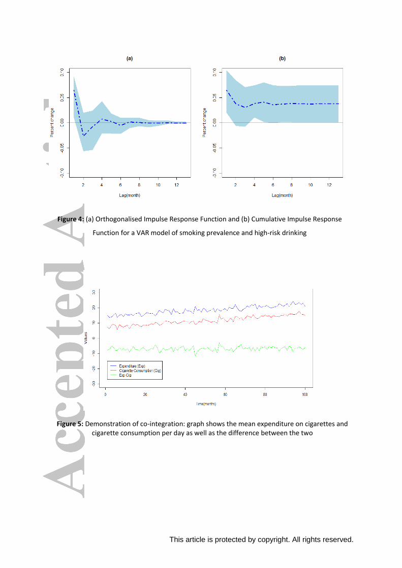
Orthogonalised Impulse Response Functions (OIRF) are usually plotted to assess how an event
affects current and future values of one or more output variables. Figure 4 gives a graphical
representation of the OIRF for a VAR model using simulated data to assess the association between

This article is protected by copyright. All rights reserved.
smoking prevalence and prevalence of high-risk drinking. The OIRF shows the change in the
prevalence of high-risk drinking in response to a change in smoking prevalence in the same month
and in the subsequent months. The dashed blue line represents the estimate at different time lags,
and the shaded area is the 95% confidence interval. The IRF suggests that there is an effect of
smoking prevalence on high-risk drinking prevalence in the same period. A cumulative IRF can also
be derived which shows the overall effect of an event (i.e. the total change in the response variable
following a change in the input variable at different time lags).
Structural Vector Autoregressive models
VAR models only use the lags of one series and may therefore miss valuable information when
‘instantaneous’ causality is present (i.e. values in one variable influence values in another within
the same observation period). As a solution, Structural Vector Autoregressive Models (SVAR) helps
to model the temporal relationships between series and place restrictions so that relationships can
be specified in a unidirectional manner. The analysis proceeds following the generation of
stationary data with the specification of a matrix which contains parameter constraints. In simple
two-series TSA the matrix is generally specified as:
[𝑋 → 𝑋 𝑌 → 𝑋𝑋 → 𝑌 𝑌 → 𝑌
]
If the aim is only to assess the relationship from X to Y, it is assumed that the effect of X on X and Y on
Y is 1, and the effect of Y on X is 0. Therefore, the only parameter that needs to be estimated is XY.
This would be appropriate for a unidimensional model for the evaluation of tobacco and alcohol
control policies when it can be assumed that causal relationships run from the policy to the outcome
but not from the outcome to the policy.
As with VAR analysis, appropriate lags which account for the presence of autocorrelation can be
assessed by comparing models using measures of goodness of fit (83). The output is also in the
form of an impulse response function, which indicates how a change in the variable X affects future
values of Y. SVAR was used recently to evaluate the effect of tobacco control media campaigns and
pharmaceutical company-funded advertising for nicotine replacement therapy on smoking
cessation activity (7).
Vector Error Correction Models
VAR and SVAR models are not suitable in the presence of ‘co-integrating relationships’. This
phenomenon arises when two variables share a common trend, and the linear combination of the
variables is stationary. For example, the number of cigarettes smoked per day and amount spent on

This article is protected by copyright. All rights reserved.
cigarettes per day may both exhibit a downward trend over time. Because both series are driven by
the same trend, the consumption/expenditure ratio will fluctuate about a constant mean i.e. the
difference between series has no obvious trend. This is shown graphically in Figure 5. Co-integrating
relationships can be addressed by re-parameterising the VAR/SVAR model as a Vector Error
Correction Model (VECM).
The presence of co-integrated variables can be tested using the Johansen procedure (84). This tests
the null hypothesis that the test statistic is equal to 0 (i.e. that there is no co-integration at all). If
co-integration had been present, then a VECM model would be run and an impulse response
functions obtained. VECM has been used in the addictions field to assess the relationship between
alcohol advertising, price and consumption, and to monitor illicit psychostimulants and related
health issues (85, 86).
Table 1 gives an overview of the key analysis types, what they are used for, required sample sizes,
statistical packages that can be used in R and what assumptions must be met. Tables 2 and 3 give
an overview of the stages in GAMM/ARIMA/ARIMAX and VAR/SVAR/VECM, respectively.
Stages in time series analysis with autocorrelations
Eight stages are proposed for GAMM and ARIMA/ARIMAX modelling: 1) assess the presence of
autocorrelation, 2) assess the presence of seasonality, 3) determine if the series is stationary (for
ARIMAX), 4) identify the number of AR and/or MA terms, 5) identify lags, 6) select the baseline
model, 7) run the model and check for additional autocorrelation and 8) check the assumption of
normality, significance of autocorrelation terms and whether they are in the bounds of invertibility
and stationarity.
Seven stages are proposed for VAR/SVAR/VECM modelling: 1) determine if the series is stationary,
2) identify the number of lags, 3) run the model and assess additional autocorrelation, 4) check the
assumption of normality of the residuals, 5) visualise the dynamic relationships, 6) check for
causality and 7) check for the presence of co-integrated variables.
PART 4: REPORTING TSA
There are several useful guides to reporting TSA, including an extension of the ‘Strengthening the
Reporting of Observational Studies in Epidemiology’ (STROBE) guideline (34, 87, 88). In this part of
the paper we extend these to more types of TSA and focus on examples in the field of addiction. A
summary of our guidelines is provided in Table 4.

This article is protected by copyright. All rights reserved.
Statistical analysis plans and related protocols should be registered online prior to data analysis (e.g.
using Open Science Framework (http://osf.io/) or AsPredicted (http://AsPredicted.org/) (89).
Changes to the analyses, and additional analyses undertaken after seeing any results should be
added to that record.
Research reports should include, as a minimum, information on stationarity, seasonality,
autocorrelation, lags and criteria for model fit. For interrupted time series designs additional
information is required in terms of the intervention time point, number of data points pre- and post-
intervention and use of a graphical display with the time points clearly defined.
Coefficients are interpreted in a similar way to those from a simple regression model except when
the data have been made stationary prior to data analysis. Interpretation also depends on whether a
log transformation or equivalent has been performed. As an example, Table 5 provides a set of
standard interpretations of coefficients under different log transformation scenarios in the presence
of stationary data. For example, when the input and output time series have been log transformed
using a natural log transformation and the data made stationary we can interpret the coefficients in
terms of elasticity i.e. a change of 1% from the overall mean value in the input series leads to a β %
change from the overall mean in the output series.
Researchers should also consider the use of Bayes Factors to help in the interpretation of null
findings. In frequentist statistics, it is not justified to argue that a ‘non-significant’ finding provides
evidence for the null hypothesis. Jeffreys (90) has proposed that we regard a Bayes Factor of less
than 1/3rd as providing strong evidence that the null hypothesis is more likely than the experimental
hypothesis, and a Bayes Factor between 1/3rd and 3 as meaning that the data are insensitive. Several
software packages are available for the calculation of Bayes Factors including an online calculator
(91) and R code (92). Both approaches require the specification of an expected effect size (i.e. a
plausible range of predicted values based on previous studies, judgement or clinical significance), the
obtained effect size (e.g. mean difference or log odds ratio) and standard error of this parameter.
For further details see (93).
DISCUSSION
Apart from simple trend analyses, there are two main types of TSA: 1) interrupted TSA which are
used to assess the impact of interventions, events or policies on a time series and 2) multiple TSA
which aim to assess how two or more time series co-vary. Both have several components that need
to be considered in the analysis process including the presence of autocorrelation, seasonality and

This article is protected by copyright. All rights reserved.
lags, and the need for log transformations and differencing to ensure stationarity in the mean and
variance.
This paper started by considering regression methods which are appropriate for analyses in the
absence of autocorrelation. For interrupted time series designs in the presence of autocorrelation,
ARIMA and GAMM are commonly used. Factors to consider when deciding between these two
options include the nature of the effect (e.g. step level change or pulse effect), and the use of pre-
aggregated versus individual level data. It is more appropriate to use individual level data when
there is reason to believe that the intervention does not have the same uniform effect across all
cases. ARIMAX is widely used for multiple TSA as it better accounts for autocorrelation. VAR, SVAR
or VECM are increasingly widely used for multiple time series and are required when there may be
bidirectional causal associations between variables.
We have not covered the use of time series data for forecasting, nor have we covered methods of
validating models. For forecasting, ARIMA/ARIMAX and VAR models are commonly used (41). It
should also be noted that other approaches exist for the analysis of time series data that are
beyond the scope of this paper (see (35, 87, 94). These other related types of analysis include the
use of simultaneous or structural equation models (SEQ) (83) and ARIMA in conjunction with a
Generalised AutoRegressive Conditional Heteroscedasticity (GARCH) models. The latter removes
the need for the assumption of constant variance over-time, but optimisation problems are
common (95).
Random Forest regression, based on decision trees, is also widely reported in the machine learning
literature (96). For single case intervention analysis, the interrupted time series experiment (ITSE)
method has been proposed, although it has major limitations (97). Latent growth curve modelling
provides another useful method for analysing intervention effects on individual cases (98) and
aggregated time series (99). Use of artificial neural networks has also been suggested as a method
for TSA which can capture non-linearity and chaotic behaviour (100). Finally, periodograms and
spectral analysis can be used to identify complex cycles and seasonality in the data (101).
Funding
No funders had any involvement in the writing of this report or the decision to submit the paper for
publication. EB, JB & IT salaries are funded by a programme grant from Cancer Research UK (CRUK;
C1417/A22962). EB and SM receive support from National Institute for Health Research (NIHR)
SPHR2. SPHR is a partnership between the Universities of Sheffield; Bristol; Cambridge; Imperial
College London; UCL; The London School for Hygiene and Tropical Medicine; the LiLaC collaboration

This article is protected by copyright. All rights reserved.
between the Universities of Liverpool and Lancaster and Fuse; The Centre for Translational
Research in Public Health, a collaboration between Newcastle, Durham, Northumbria, Sunderland
and Teesside Universities. JM has a part-time position as Senior Academic Advisor to the Division of
Alcohol, Drugs, Tobacco and Justice Division of Public Health England. The views expressed are
those of the authors(s) and not necessarily those of the Department of Health, PHE, or NIHR.
This article is protected by copyright. All rights reserved.
Figure 1: Decomposition of time series data for a hypothetical series of prevalence of excessive
alcohol consumption in a population

This article is protected by copyright. All rights reserved.
Figure 2: Hypothetical time series data for excessive alcohol consumption after (a) a log
transformation and (b) first order differencing to remove non-stationarity
Figure 3: ACF and PACF for excessive alcohol consumption after differencing
This article is protected by copyright. All rights reserved.
Figure 4: (a) Orthogonalised Impulse Response Function and (b) Cumulative Impulse Response
Function for a VAR model of smoking prevalence and high-risk drinking
Figure 5: Demonstration of co-integration: graph shows the mean expenditure on cigarettes and cigarette consumption per day as well as the difference between the two

This article is protected by copyright. All rights reserved.
Table 1: Summary of TSA features
TSA model
Used for R packages Level of data analysis
Variable type of output series
Autocorrelation Seasonality adjustment
Sample size Assumptions
GLMM Trend analysis and interrupted time series analysis; can also assess multiple time series if there are no lag effects
‘glmm’(102) ‘lme4’ (103) ‘nlme’(104)
Individual Any Can account for MA and AR autocorrelation
Seasonal index, seasonal dummy variable or natural cubic splines
Fewer than 50 data points leads to biased estimates (105, 106). If data are at the individual level sample size should be at least 100 participants per time point (106).
Standard regression assumptions apply e.g. normally distributed errors
GLS Trend analysis and interrupted time series analysis; can also assess multiple time series if there are no lag effects
‘nlme’(104) Individual or aggregated
Any Can account for MA and AR autocorrelation
Seasonal index, seasonal dummy variable or natural cubic splines
Fewer than 50 data points leads to biased estimates (105, 106). If data are at the individual level sample size should be at least 100 participants each time point (106).
Standard regression assumptions apply as for GLMM with the Gaussian distribution.
GAMM Trend analysis and interrupted time series analysis; can also assess multiple time series if there are no lag effects
‘mgcv’ (107) ‘gamm4’ (108)
Individual or aggregated
Any Can account for MA and
AR autocorrelation
Seasonal index,
seasonal dummy
variable or natural
smoothing terms
Large sample sizes required as for generalised
linear mixed models, but larger if smoothing
terms are used with multiple knots e.g. 12
knots are used for 12 months generally (109).
Sample size at lower level has a smaller impact,
though at least 100 participants are
recommended (106).
As GAMM are semi-parametric
extensions of GLMs; the only
underlying assumption made is that
the functions are additive and that
the components are smooth.
ARIMA Trend analysis and interrupted time series analysis
‘forecast’ (110)
Aggregated Continuous Can account for both
seasonal and non-
seasonal MA and AR
autocorrelation
Accounted for
through seasonal
differencing and the
use of seasonal MA
and AR terms
Some have recommended at least 50-100
observations in total (31, 32), while others have
argued that short-time series data can be used
so long as there are more observation periods
than parameters (33).
Standard parametric assumptions
e.g. linearity, multicollinearity and
heteroscedasticity as well as
stationarity and invertibility.
ARIMAX Multiple time series analysis; can also add interrupted time series as covariates
‘TSA’ (111) Aggregated Continuous Can account for both
seasonal and non-
seasonal MA and AR
autocorrelation
Accounted for
through seasonal
differencing and the
use of seasonal MA
and AR terms
Some have recommended at least 50-100
observations in total (31, 32), while others have
argued that short-time series data can be used
so long as there are more observation periods
than parameters (33).
Same as for ARIMA plus the
assumption of weak exogeneity.
VAR Multiple time series analysis with bidirectional causation between input and output variables
‘vars’ (112) Aggregated Continuous Does not include MA terms, but approximates any existing MA patterns with extra AR lags
Seasonal dummy variables can be added as exogenous variables
Similar sample size to ARIMAX models, with a large number of data points required if a seasonal dummy variable is included.
VAR and SVAR are not suitable in the presence of co-integrating relationships
VECM Multiple time series analysis with bidirectional causation between input and output variables
‘tsDyn’ (113) Aggregated Continuous Does not include MA terms, but approximates any existing MA patterns with extra AR lags
Seasonal dummy variables can be added as exogenous variables
Similar sample size to ARIMAX models, with a large number of data points required if a seasonal dummy variable is included.
VAR and SVAR are not suitable in the presence of co-integrating relationships
SVAR Multiple time series analysis ‘vars’(112) Aggregated Continuous Does not include MA Seasonal dummy Similar sample size to ARIMAX models, with a VAR and SVAR are not suitable in the

This article is protected by copyright. All rights reserved.
with bidirectional causation between input and output variables
terms, but approximates any existing MA patterns with extra AR lags
variables can be added as exogenous variables
large number of data points required if a seasonal dummy variable is included.
presence of co-integrating relationships

This article is protected by copyright. All rights reserved.
Table 2: Steps in TSA for GAMM/ARIMA/ARIMAX models
Step Method Multiple time series Interrupted time series
Assess the presence of autocorrelation
Simple lag-1 autocorrelation can be detected with the use of the Durbin Watson statistic. For more complex patterns, the Autocorrelation Function (ACF) and Partial Autocorrelation Function (PACF) should be referred to.
No autocorrelation Simple regression Autocorrelation ARIMAX
No autocorrelation Simple regression Autocorrelation GAMM if limited number of data points, only interested in step level effects and want to assess moderation of individual level variables. ARIMA if long time series and interested in differing patterns of effects (e.g. pulse, step and delayed effects).
Assess the presence of seasonality
Plot of the raw time series data and use the ACF and PACF. Look for significant lags at seasonal points (e.g. lag 4 and 8 for quarterly data) in the later, and cyclical patterns in the former.
No seasonal effects Simple regression if no autocorrelation. ARIMAX if autocorrelation is present Seasonal effects Simple regression with a cubic spline if no autocorrelation (STOP). ARIMAX if autocorrelation is also present.
No seasonal effects Simple regression if no autocorrelation. GAMM if autocorrelation is present and you have limited number of data points, only interested in step level effects and want to assess moderation of individual level variables. ARIMA if autocorrelation is present and you have a long-time series and interested in differing patterns of effects (e.g. pulse, step and delayed effects). Seasonal effects Simple regression with a cubic spline if no autocorrelation. GAMM if autocorrelation is present and you have limited number of data points, only interested in step level effects and want to assess moderation of individual level variables. ARIMA if autocorrelation is present and you have a long-time series and interested in differing patterns of effects (e.g. pulse, step and delayed effects).
Determine if the series is stationary
If autocorrelation is present, check if the series is stationary. This can be done by using unit root tests and visually inspecting the series graphically
If the variance is not constant over time, consider a natural logarithmic transformation. If the mean is not constant over time, difference the data. Consider both seasonal and non-seasonal differencing.
If the variance is not constant over time, consider a natural logarithmic transformation. If the mean is not constant over time, difference the data. Consider both seasonal and non-seasonal differencing.
Identify the number of AR and MA terms
The ACF and PACF can be used to determine the number of autocorrelation terms required.
A steadily decaying ACF and a PACF that drops after p lags would be consistent with an AR term. In contrast, an MA term would be consistent with a ACF that drops off after q lags and a gradual decay in the PACF.
A steadily decaying ACF and a PACF that drops after p lags would be consistent with an AR term. In contrast, an MA term would be consistent with a ACF that drops off after q lags and a gradual decay in the PACF.
Identify any lags This can be done by comparing models with different lag effects using the AIC. For multiple time series analysis, the CCF can be used.
If there is evidence of lag effect include this in the ARIMAX model by specifying a transfer function.
If there are no lag effects continue with the chosen analysis, if there is evidence of a lag effect consider using ARIMA models.
Select the baseline model
Run the baseline model with the input series (and covariates) included and compare with other models using the AIC
If other models provide a better fit, consider these over the baseline model.
If other models provide a better fit, consider these over the baseline model.
Run the model and check for additional autocorrelation
Examine the model residuals and check the Ljung-Box test
If the residuals form a random pattern and the Ljung-Box test is non-significant do not change model. If a pattern remains and there is evidence of further autocorrelation consider adding additional seasonal or non-seasonal AR and MA terms.
If the residuals form a random pattern and the Ljung-Box test is non-significant do not change model. If a pattern remains and there is evidence of further autocorrelation consider adding additional seasonal or non-seasonal AR and MA terms. The latter of which can only be added to ARIMA models.
Check the assumption of normality, significance of autocorrelation terms
These can be checked with q-q plots and assessing the size and significance of
If MA and AR terms do not contribute significantly or violate the assumption of bounds of invertibility and stationarity remove from the analysis.
If MA and AR terms do not contribute significantly or violate the assumption of bounds of invertibility and stationarity remove from the analysis.

This article is protected by copyright. All rights reserved.
and within bounds of invertibility and stationarity.
coefficients.

This article is protected by copyright. All rights reserved.
Table 3: Steps in a VAR/SVAR/VECM
Step Method
Determine if the series is stationary If autocorrelation is present, check if the series is stationary. This can be done by using unit root tests and visually inspecting the series graphically
Identify the number of lags This can be done by comparing models with different lag effects using the AIC.
Run the model and assess additional autocorrelation
Autocorrelation among the residuals assessed using a Portmanteau test
Check the assumption of normality of residuals
This can be done using the Jarque-Bera normality tests for multivariate series
Visualise the equations Calculate the impulse response function and cumulative impulse response function
Check for causality Run the Granger causality test and instant causality test
Check for the presence of co-integrated variables
Run the Johansen procedure.

This article is protected by copyright. All rights reserved.
Table 4: Guidelines for the reporting of TSA
Item Recommendation
Title (a) Indicate the type of TSA e.g. trend analysis, interrupted TSA, multiple TSA or forecasting
(b) Indicate the study design e.g. repeated cross-sectional, open cohort or longitudinal cohort
(c) Indicate the study population e.g. population sample of those in England
Abstract (a) Provide an informative summary of what was done with reference to: a. Type of TSA b. Study design c. Study population
(b) Report relevant coefficients with confidence intervals and p-values (c) Provide a balanced conclusion based on correlational not causal statements
Introduction (a) Explain the rationale and background for conducting the TSA analysis (b) Clearly state the specific objectives, including pre-specified hypotheses (these
should be pre-registered on the Open Science Framework or equivalent along with the analysis plan)
Methods Study design Participants Measures Sample size
(a) Clearly state the study design and all data sources including dates of data
collection and a statement on data access (b) Comment on change in data sources over time (a) If data are initially collected at the individual level give eligibility criteria and
method of selection and recruitment. If data are collected at the aggregated level give eligibility criteria
(a) Define all independent variables e.g. input series for multiple TSA and dummy coded intervention variables for interrupted TSA
(b) Define all dependent variables i.e. the output series (c) Define all covariates/confounding variables adjusted for in the study (d) Define any moderators or stratified variables (a) Explain how the sample size was arrived at and if it is adequate in terms of the
length of the series and the number of data points within each wave if at the individual level
Statistical analysis (a) The analysis plan should be pre-registered on the Open Science Framework or equivalent along with objectives and hypotheses. Changes and extension to the analysis should be recorded
(b) Report statistical software and packages used for the analysis (c) Explain how missing data and outliers will be assessed, reasons for them, and
how they will be handled e.g. deletion, multiple imputation or last one carried forward
(d) Explain how seasonality, autocorrelation and lags will be assessed (e.g. indices of fit such as the AIC and BIC, PACF and ACF, CCF) and addressed (e.g. seasonal index, cubic splines, smoothing terms, seasonal and non-seasonal AR and MA terms and transfer functions)
(e) Describe the statistical analysis and how assumptions will be assessed a. Parametric (e.g. for GLMM/ARIMA/ARIMAX) – normally distributed
errors, linearity and homoscedasticity b. Multicollinearity for all analyses c. Stationarity (e.g. ARIMAX/ARIMA) d. Weak exogenenity (e.g. ARIMAX/VAR/SVAR/VECM) e. Bound of stationarity and invertibility (e.g. ARIMA/ARIMAX) f. Cointegration (e.g. VECM)

This article is protected by copyright. All rights reserved.
Table 4: Guidelines for the reporting of TSA (continued)
Item Recommendation
Statistical analysis (a) Describe how violations of the assumptions will be handled a. Transformations e.g. log transformation for stationarity and parametric
assumptions b. Differencing for stationarity c. Selection methods for multicollinearity d. Other analysis options
(b) (64, 93)Consider the calculation of Bayes Factors to aid interpretation of null findings (64, 93)
(c) State all underlying assumptions (d) State any unplanned sensitivity analyses and the reasons for them (e) Explain how any continuous variables were categorised for the analysis and
comment on changes in variable coding over time (f) Give guidelines on the interpetation of coefficients taking into account
transformations of the data (see Table 5 for examples)
Results Participants Descriptive statistics Main results Other analysis Visual displays
(a) If data are available at the individual level report the total number taking part in
the study (and the average number recruited at each stage if cross-sectional). For cohort studies give details on those lost to follow up.
(a) If data are available at the individual level report characteristics e.g. demographic. If data are available at the aggregated level report the start, end and average values of each series in the analysis
(b) Provide graphical figures of the aggregated data over time (a) Give adjusted and unadjusted estimates and their precision e.g. 95% confidence
interval and, if applicable, Bayes Factors (b) Specify the final model e.g. AR and MA terms, order of differencing and presence
of lags (a) Report any analyses e.g. moderation, subgroup and unplanned sensitivity (a) Present results using a graphical display with intervention time point(s) clearly
defined for interrupted time series
Discussion Key results Limitations Interpretation Implications/future research
(a) Summaries the main findings with reference to the study objectives and aims (a) Discuss all limitations of the study with a focus on possible bias and imprecision (a) Give a cautious overall interpretation of results relating them to previous studies (a) Discuss the possible implications of the findings in relation to policy, clinical
objectives etc (b) Consider avenues for future research
Other information Funding Ethical approval Conflicts of interest
(a) Gives sources of funding for the study (a) Explain if ethical approval was sought and how (a) Clearly state any conflicts of interest in relation to the paper

This article is protected by copyright. All rights reserved.
Table 5: Interpretation of coefficients for predictors in GAMM/ARIMA/ARIMAX/VAR models with
stationary data
Predictor variable Dependent variable Interpretation
Binary (dummy) Continuous The introduction of X resulted in a β units change in the average of Y
Continuous Continuous For every one-unit change in the average of X, the average of Y changes by β units
Log transformed continuous Continuous A one percent change in the average of X leads to a
β × ln (101
100) [~ 𝛽/ 100] change in the average value of Y
Binary (dummy) Log transformed continuous The introduction of X resulted in a (𝑒𝛽 − 1) ×
100 [~ 𝛽 x 100] percentage change in the average value of Y
Continuous Log transformed continuous A one percent change in the average of X leads to a
(𝑒𝛽 − 1) × 100 [~ 𝛽 x 100] percentage change in the
average value of Y
Log transformed continuous Log transformed continuous A one percent change in the average of X leads to a
(1.01𝛽 − 1) × 100 [~ 𝛽] percentage change in the
average value of Y
Note: for ARIMA/ARIMAX models which are stationary i.e. have a constant mean and variance over time, interpretation is in terms of the series mean e.g. for a log-log model a 1% change in the mean of series y leads to a β% change in the mean of series of X.

This article is protected by copyright. All rights reserved.
Appendix A: Glossary
Aggregated data: Groups of observations are replaced with summary measures.
ARIMA (Autoregressive Integrated Moving Average): a form of regression analysis that seeks to
predict future trends whilst taking into account underlying trends, seasonality and autocorrelation.
Can be extended to assess the effect of policies or interventions in an interrupted time series design.
ARIMAX (Autoregressive Integrated Moving Average with Exogeneous Input): a form of regression
analysis which seeks to assess how two time series covary whilst taking into account underlying
trends, seasonality and autocorrelation.
Autocorrelation: Estimates or regression residuals at one time point are correlated with the
estimates or residuals at a subsequent time point.
Co-integrating relationship: Two variables share a common stochastic trend in such a way that a
linear combination of the variables is stationary.
Differencing: A means by which to make a time series stationary by transforming the series into on
made up of the difference between values at time t and values at time t+n.
GAM (Generalised Additive Model): Is a generalized linear model which uses an additive modelling
technique where the impact of the predictive variables is captured through smooth functions.
GLS (Generalised Least Squares): A statistical technique that allows one to perform linear regression
when there is a certain degree of autocorrelation between the residuals.
GLMM (Generalised Linear Mixed Model): An extension to GLM (see below) which contains random
effects to account for clustering.
GLM (Generalised Linear Model): A flexible generalization of linear regression that allows for
response variables that have error distributions other than a normal distribution.
Parametric test: Makes assumptions about the parameters of the population distribution(s) from
which one's data are taken. Non-parametric tests are often referred to as ‘distribution-free’ tests.
Polynomial terms: Relationships between the independent variable and the dependent variable is
modelled as an nth degree polynomial e.g. quadratic (^2) and cubic (^3).
Smoothing spline: Provide a flexible way of representing the relationship between two variables
involving fitting of piecewise polynomial terms with breakpoints or changes in the strength and
direction of the association.
Stationary: A stationary time series is one whose properties do not depend on the time at which the
series is observed. So, a time series with trends or with seasonality cannot be stationary as they will
affect the value of the time series at different times. In general, a stationary time series will have no
predictable patterns in the long-term.

This article is protected by copyright. All rights reserved.
SVAR (Structural Vector Autoregressive Model): An extension of VAR (see below) that helps to
model the temporal relationships between series by placing restrictions so that relationships can be
specified in a unidirectional manner.
VAR (Vector Autoregression): A model that allows specification of bi-directional causal associations
between two time series.
Vector Error Correction Model (VECM): An extension of SVAR and VAR which is used in the presence
of co-integrating relationships.
Pre-whitening: A procedure that converts an input series into one with a mean of zero and no
autocorrelation and applies the same transformation to an output series.
Weak exogeneity: An assumption of ARIMAX models which specifies that there is no reverse causal
pathway with the output series having an effect on any of the input variables.
White noise: A white noise series has a mean of zero and no autocorrelation.
REFERENCES
1. Kothari SP, Shanken J. Book-to-market, dividend yield, and expected market returns: A time-series analysis. Journal of Financial Economics. 1997;44(2):169-203. 2. Montgomery DC, Johnson LA, Gardiner JS. Forecasting and time series analysis: McGraw-Hill Companies; 1990. 3. Montgomery DC, Jennings CL, Kulahci M. Introduction to time series analysis and forecasting: John Wiley & Sons; 2015. 4. Cryer JD, Chan K-S. Time series analysis - with applications in R. London: Springer-Verlag New York; 2008. 5. Dierker L, Stolar M, Lloyd-Richardson E, Tiffany S, Flay B, Collins L, et al. Tobacco, alcohol, and marijuana use among first-year U.S. college students: a time series analysis. Subst Use Misuse. 2008;43(5):680-99. 6. Beard E, Brown J, McNeill A, Michie S, West R. Has growth in electronic cigarette use by smokers been responsible for the decline in use of licensed nicotine products? Findings from repeated cross-sectional surveys. Thorax. 2015:thoraxjnl-2015-206801. 7. Langley TE, McNeill A, Lewis S, Szatkowski L, Quinn C. The impact of media campaigns on smoking cessation activity: a structural vector autoregression analysis. Addiction. 2012;107(11):2043-50. 8. Brunt TM, van Laar M, Niesink RJ, van den Brink W. The relationship of quality and price of the psychostimulants cocaine and amphetamine with health care outcomes. Drug and alcohol dependence. 2010;111(1-2):21-9. 9. Holder HD, Wagenaar AC. Mandated server training and reduced alcohol-involved traffic crashes: a time series analysis of the Oregon experience. Accident Analysis & Prevention. 1994;26(1):89-97. 10. Kuipers MAG, Beard E, Hitchman SC, Brown J, Stronks K, Kunst AE, et al. Impact on smoking of England's 2012 partial tobacco point of sale display ban: a repeated cross-sectional national study. Tobacco Control. 2016. 11. Langley T, Szatkowski L, Lewis S, McNeill A, Gilmore AB, Salway R, et al. The freeze on mass media campaigns in England: a natural experiment of the impact of tobacco control campaigns on quitting behaviour. Addiction. 2014;109(6):995-1002.

This article is protected by copyright. All rights reserved.
12. Langley TE, Huang Y, McNeill A, Coleman T, Szatkowski L, Lewis S. Prescribing of smoking cessation medication in England since the introduction of varenicline. Addiction. 2011;106(7):1319-24. 13. Humphreys DK, Eisner MP, Wiebe DJ. Evaluating the Impact of Flexible Alcohol Trading Hours on Violence: An Interrupted Time Series Analysis. PLoS ONE. 2013;8(2):e55581. 14. Robinson M, Geue C, Lewsey J, Mackay D, McCartney G, Curnock E, et al. Evaluating the impact of the alcohol act on off-trade alcohol sales: a natural experiment in Scotland. Addiction (Abingdon, England). 2014;109(12):2035-43. 15. Slováčková T, Birčiaková N, Stávková J. Forecasting Alcohol Consumption in the Czech Republic. Procedia - Social and Behavioral Sciences. 2016;220:472-80. 16. Wang H, Preston SH. Forecasting United States mortality using cohort smoking histories. Proceedings of the National Academy of Sciences. 2009;106(2):393-8. 17. Hasse B, Tarr PE, Marques-Vidal P, Waeber G, Preisig M, Mooser V, et al. Strong Impact of Smoking on Multimorbidity and Cardiovascular Risk Among Human Immunodeficiency Virus-Infected Individuals in Comparison With the General Population. Open Forum Infectious Diseases. 2015;2(3):ofv108. 18. Collins GS, Altman DG. An independent and external validation of QRISK2 cardiovascular disease risk score: a prospective open cohort study. BMJ. 2010;340. 19. Marston L, Carpenter JR, Walters KR, Morris RW, Nazareth I, White IR, et al. Smoker, ex-smoker or non-smoker? The validity of routinely recorded smoking status in UK primary care: a cross-sectional study. BMJ Open. 2014;4(4). 20. Vincent KB, Kasperski SJ, Caldeira KM, Garnier-Dykstra LM, Pinchevsky GM, O’Grady KE, et al. Maintaining Superior Follow-Up Rates in a Longitudinal Study: Experiences from the College Life Study. International journal of multiple research approaches. 2012;6(1):4406. 21. Kumar S, Nilsen WJ, Abernethy A, Atienza A, Patrick K, Pavel M, et al. Mobile health technology evaluation: the mHealth evidence workshop. American journal of preventive medicine. 2013;45(2):228-36. 22. Shusterman V, Goldberg A, London B. Upsurge in T-wave alternans and nonalternating repolarization instability precedes spontaneous initiation of ventricular tachyarrhythmias in humans. Circulation. 2006;113(25):2880-7. 23. Hedeker D, Demirtas H, Mermelstein RJ. A mixed ordinal location scale model for analysis of Ecological Momentary Assessment (EMA) data. Statistics and its Interface. 2009;2(4):391. 24. Vieira R, McDonald S, Araújo-Soares V, Sniehotta FF, Henderson R. Dynamic modelling of n-of-1 data: powerful and flexible data analytics applied to individualised studies. Health Psychology Review. 2017;11(3):222-34. 25. Beard E, Brown J, Michie S, West R. Using time-series analysis to examine the effects of adding or removing components of digital behavioural interventions and associations between outcomes and patterns of usage. Frontiers in Public Health. 26. Zhang F, Wagner AK, Ross-Degnan D. Simulation-based power calculation for designing interrupted time series analyses of health policy interventions. Journal of clinical epidemiology. 2011;64(11):1252-61. 27. Erdfelder E, Faul F, Buchner A. GPOWER: A general power analysis program. Behavior research methods, instruments, & computers. 1996;28(1):1-11. 28. Faul F, Erdfelder E, Buchner A, Lang A-G. Statistical power analyses using G* Power 3.1: Tests for correlation and regression analyses. Behavior research methods. 2009;41(4):1149-60. 29. McLeod AI, Vingilis ER. Power Computations for Intervention Analysis. Technometrics : a journal of statistics for the physical, chemical, and engineering sciences. 2005;47(2):174-81. 30. McLeod AI, Vingilis ER. Power Computations in Time Series Analyses for Traffic Safety Interventions. Accident; analysis and prevention. 2008;40(3):1244-8. 31. Yaffee R. An Introduction to Forecasting Time Series with Stata. Taylor & Francis; 2012.

This article is protected by copyright. All rights reserved.
32. EPOC. Including Interrupted Time Series (ITS) designs in EPOC review: the Cochrane effective practice and organisation of care group. 1998. 33. Hyndman RJ, Kostenko AV. Minimum sample size requirements for seasonal forecasting models. Foresight. 2007;6(Spring):12-5. 34. Wagner AK, Soumerai SB, Zhang F, Ross‐Degnan D. Segmented regression analysis of interrupted time series studies in medication use research. Journal of clinical pharmacy and therapeutics. 2002;27(4):299-309. 35. Box GE, Jenkins GM, Reinsel GC, Ljung GM. Time series analysis: forecasting and control: John Wiley & Sons; 2015. 36. Hyndman RJ, Athanasopoulos G. Forecasting: principles and practice: OTexts; 2014. 37. Anderson OD. Time series analysis and forecasting: the Box-Jenkins approach: Butterworths London; 1976. 38. Cowpertwait PS, Metcalfe AV. Introductory time series with R: Springer Science & Business Media; 2009. 39. Fuller WA. Introduction to statistical time series: John Wiley & Sons; 2009. 40. Phillips PC, Perron P. Testing for a unit root in time series regression. Biometrika. 1988:335-46. 41. McCleary R, Hay RA, Meidinger EE, McDowall D. Applied time series analysis for the social sciences: Sage Publications Beverly Hills, CA; 1980. 42. Lütkepohl H, Xu F. The role of the log transformation in forecasting economic variables. Empirical Economics. 2012;42(3):619-38. 43. Box GE, Jenkins GM, Reinsel GC. Time series analysis: forecasting and control: John Wiley & Sons; 2011. 44. Beard E, West R, Michie S, Brown J. Association between smoking and alcohol-related behaviours: A time-series analysis of population trends in England. Addiction.n/a-n/a. 45. Schünemann H, Hill S, Guyatt G, Akl EA, Ahmed F. The GRADE approach and Bradford Hill's criteria for causation. Journal of Epidemiology & Community Health. 2010:jech. 2010.119933. 46. Chernick MR, Downing DJ, Pike DH. Detecting outliers in time series data. Journal of the American Statistical Association. 1982;77(380):743-7. 47. Chen C, Liu L-M. Joint estimation of model parameters and outlier effects in time series. Journal of the American Statistical Association. 1993;88(421):284-97. 48. López-de-Lacalle J. R Package tsoutliers. 2017. 49. Jesús Sánchez M, Peña D. The identification of multiple outliers in ARIMA models. Communications in Statistics-Theory and Methods. 2003;32(6):1265-87. 50. Beard E, West R, Michie S, Brown J. Association between smoking and alcohol‐related behaviours: a time–series analysis of population trends in England. Addiction. 2017;112(10):1832-41. 51. Velicer WF, Colby SM. A comparison of missing-data procedures for ARIMA time-series analysis. Educational and Psychological Measurement. 2005;65(4):596-615. 52. Rubin DB. Multiple imputation for nonresponse in surveys: John Wiley & Sons; 2004. 53. Honaker J, King G, Blackwell M. Amelia II: A program for missing data. Journal of Statistical Software. 2011;45(7):1-47. 54. Buuren Sv, Groothuis-Oudshoorn K. mice: Multivariate imputation by chained equations in R. Journal of statistical software. 2010:1-68. 55. Templ M, Alfons A, Kowarik A, Prantner B. VIM: visualization and imputation of missing values. R package version. 2011;2(3). 56. Kihoro Y, Athiany J, Kibunja K. Imputation of incomplete non-stationary seasonal time series. Math Theory Model. 2013;3:142154. 57. Moritz S, Bartz-Beielstein T. imputeTS: time series missing value imputation in R. The R Journal. 2017;9(1):207-18. 58. Bloomfield P. Fourier analysis of time series: an introduction: John Wiley & Sons; 2004.

This article is protected by copyright. All rights reserved.
59. Sims CA. Seasonality in regression. Journal of the American Statistical Association. 1974;69(347):618-26. 60. Perrakis K, Gryparis A, Schwartz J, Le Tertre A, Katsouyanni K, Forastiere F, et al. Controlling for seasonal patterns and time varying confounders in time-series epidemiological models: a simulation study. Stat Med. 2014;33(28):4904-18. 61. Lemon D, Partridge R. Is weather related to the number of assaults seen at emergency departments? Injury. 2017;48(11):2438-42. 62. Park RE, Mitchell BM. Estimating the autocorrelated error model with trended data. Journal of Econometrics. 1980;13(2):185-201. 63. Kerr WC, Ye Y. Beverage-specific mortality relationships in US population data. Contemporary drug problems. 2011;38(4):561-78. 64. Dienes Z. Using Bayes to get the most out of non-significant results. Frontiers in psychology. 2014;5. 65. Ugrinowitsch C, Fellingham GW, Ricard MD. Limitations of ordinary least squares models in analyzing repeated measures data. Med Sci Sports Exerc. 2004;36(12):2144-8. 66. Overall JE, Tonidandel S. Robustness of generalized estimating equation (GEE) tests of significance against misspecification of the error structure model. Biometrical Journal. 2004;46(2):203-13. 67. Koper N, Manseau M. Generalized estimating equations and generalized linear mixed‐effects models for modelling resource selection. Journal of Applied Ecology. 2009;46(3):590-9. 68. Hastie TJ, Tibshirani RJ. Generalized additive models: CRC Press; 1990. 69. Shumway RH, Stoffer DS. Time series analysis and its applications: Springer Science & Business Media; 2013. 70. Shumway RH, Stoffer DS. Time series analysis and its applications: with R examples: Springer Science & Business Media; 2010. 71. Wood S. Generalized additive models: an introduction with R: CRC press; 2006. 72. Chatfield C. The analysis of time series: an introduction: CRC press; 2013. 73. Zinszer K, Verma AD, Charland K, Brewer TF, Brownstein JS, Sun Z, et al. A scoping review of malaria forecasting: past work and future directions. BMJ Open. 2012;2(6). 74. Osborne JW. Improving your data transformations: Applying the Box-Cox transformation. Practical Assessment, Research & Evaluation. 2010;15(12):1-9. 75. Taylor JM, Yu M. Bias and efficiency loss due to categorizing an explanatory variable. Journal of Multivariate Analysis. 2002;83(1):248-63. 76. Peter Ď, Silvia P, editors. ARIMA vs. ARIMAX–which approach is better to analyze and forecast macroeconomic time series? Proceedings of the 30th International Conference Mathematical Methods in Economics Karviná, Czech Republic; 2012. 77. Granger CW. Some recent development in a concept of causality. Journal of econometrics. 1988;39(1):199-211. 78. Arjas E, Eerola M. On predictive causality in longitudinal studies. Journal of Statistical Planning and Inference. 1993;34(3):361-86. 79. Li L, Wu Z, Liang LJ, Lin C, Zhang L, Guo S, et al. An intervention targeting service providers and clients for methadone maintenance treatment in China: a cluster‐randomized trial. Addiction. 2013;108(2):356-66. 80. Landberg J, Norström T. Alcohol and Homicide in Russia and the United States: A Comparative Analysis. Journal of Studies on Alcohol and Drugs. 2011;72(5):723-30. 81. Lebo MJ, Weber C. An effective approach to the repeated cross‐sectional design. American Journal of Political Science. 2015;59(1):242-58. 82. Patilea V, Raïssi H. Corrected portmanteau tests for VAR models with time-varying variance. Journal of Multivariate Analysis. 2013;116:190-207. 83. Brandt PT, Williams JT. Multiple time series models: Sage; 2007.

This article is protected by copyright. All rights reserved.
84. Johansen S. Statistical analysis of cointegration vectors. Journal of economic dynamics and control. 1988;12(2):231-54. 85. Edward CN, Moran JR, Nelson JP. The long-run demand for alcoholic beverages and the advertising debate: A cointegration analysis. Advances in applied microeconomics. 2001;10:31-54. 86. Brunt TM. Monitoring illicit psychostimulants and related health issues: BOXPress; 2012. 87. Jandoc R, Burden AM, Mamdani M, Lévesque LE, Cadarette SM. Interrupted time series analysis in drug utilization research is increasing: systematic review and recommendations. Journal of Clinical Epidemiology. 2015;68(8):950-6. 88. Penfold RB, Zhang F. Use of Interrupted Time Series Analysis in Evaluating Health Care Quality Improvements. Academic Pediatrics.13(6):S38-S44. 89. Open Science Collaboration. An open, large-scale, collaborative effort to estimate the reproducibility of psychological science. Perspectives on Psychological Science. 2012;7(6):657-60. 90. Jeffreys H. Theory ofprobability. Oxford: Clarendon Press; 1961. 91. Dienes Z. Bayes Factor Calculator. Available from: http://www.lifesci.sussex.ac.uk/home/Zoltan_Dienes/inference/Bayes.htm. 92. Christie J. Bayes Factor Calculator. R code 2011. Available from: http://www.lifesci.sussex.ac.uk/home/Zoltan_Dienes/inference/bayesFactorCalc2.R. 93. Beard E, Dienes Z, Muirhead C, West R. Using Bayes factors for testing hypotheses about intervention effectiveness in addictions research. Addiction (Abingdon, England). 2016;111(12):2230-47. 94. Percival DB, Walden AT. Wavelet methods for time series analysis: Cambridge university press; 2006. 95. Bollerslev T. Generalized autoregressive conditional heteroskedasticity. Journal of econometrics. 1986;31(3):307-27. 96. Breiman L. Random forests. Machine learning. 2001;45(1):5-32. 97. Huitema BE, McKean JW, Laraway S. Time-series intervention analysis using ITSACORR: Fatal flaws. Journal of Modern Applied Statistical Methods. 2007;6(2):4. 98. McArdle JJ. Dynamic but structural equation modeling of repeated measures data. Handbook of multivariate experimental psychology: Springer; 1988. p. 561-614. 99. Duncan TE, Duncan SC. A latent growth curve modeling approach to pooled interrupted time series analyses. Journal of Psychopathology and Behavioral Assessment. 2004;26(4):271-8. 100. Dematos G, Boyd MS, Kermanshahi B, Kohzadi N, Kaastra I. Feedforward versus recurrent neural networks for forecasting monthly japanese yen exchange rates. Financial Engineering and the Japanese Markets. 1996;3(1):59-75. 101. Zeger SL, Irizarry R, Peng RD. On time series analysis of public health and biomedical data. Annu Rev Public Health. 2006;27:57-79. 102. Knudson C. 8 confint. glmm. Package ‘glmm’. 2018:8. 103. Bates D, Maechler M, Bolker B, Walker S. lme4: Linear mixed-effects models using Eigen and S4. R package version. 2014;1(7):1-23. 104. Pinheiro J, Bates D, DebRoy S, Sarkar D. R Core Team (2014) nlme: linear and nonlinear mixed effects models. R package version 3.1-117. Available at h ttp://CRAN R-project org/package= nlme. 2014. 105. Maas CJ, Hox JJ. Sufficient sample sizes for multilevel modeling. Methodology. 2005;1(3):86-92. 106. Snijders TA. Power and sample size in multilevel linear models. Encyclopedia of statistics in behavioral science. 2005. 107. Wood SN. mgcv: GAMs and generalized ridge regression for R. R news. 2001;1(2):20-5. 108. Wood S, Scheipl F. gamm4: Generalized additive mixed models using mgcv and lme4. R package version 0.2-3. 2014. 109. Keele LJ. Semiparametric regression for the social sciences: John Wiley & Sons; 2008.

This article is protected by copyright. All rights reserved.
110. Hyndman RJ, Athanasopoulos G, Bergmeir C, Caceres G, Chhay L, O'Hara-Wild M, et al. forecast: Forecasting functions for time series and linear models. 2018. 111. Chan K-S, Ripley B. TSA: time series analysis. R package version 1.01. URL: http://CRAN R-project org/package= TSA. 2012. 112. Pfaff B. VAR, SVAR and SVEC models: Implementation within R package vars. Journal of Statistical Software. 2008;27(4):1-32. 113. Di Narzo AF, Aznarte JL, Stigler M. Package ‘tsDyn’. 2018.