understanding and assessing logic control design …morrisonlucas.com/thesis/mrlucas_thesis.pdf ·...
TRANSCRIPT
Understanding and Assessing LogicControl Design Methodologies
by
Morrison Ray Lucas
A Dissertation submitted in partial fulfillmentof the requirements for the degree of
Doctor of Philosophy(Mechanical Engineering)
in the University of Michigan2003
Doctoral Committee
Associate Professor Dawn M. Tilbury, ChairProfessor David E. KierasProfessor Stephane LafortuneProfessor A. Galip Ulsoy

c© Morrison Ray Lucas
All rights reserved2003

Acknowledgements
I would like to acknowledge the Engineering Research Center for Reconfigurable Ma-
chining Systems (ERC/RMS) for providing the inspiration and direction for much of
this work. This would not have been possible without the support of the National
Science Foundation under grant EEC95-29125, which supported the ERC/RMS and
me throughout my graduate career.
I would also like to thank my advisor, Professor Dawn M. Tilbury, for her advice
and direction throughout my graduate career.
Finally, I would like to thank the industrial members of the ERC/RMS for their
explanations of “real world” problems. I would especially like to thank Ruven Brooks
of Rockwell, for his insight into the history and practice of control logic design; and
the engineers at Lamb Technicon, who allowed me to tag along and look over their
shoulders so that I could really understand what was going on.
ii

Table of Contents
Acknowledgements ii
List of Figures viii
List of Tables x
Chapter 1 Introduction 1
1.1 Motivation . . . . . . . . . . . . . . . . . . . . . . . . . . . . . . . . . 1
1.2 Research Approach . . . . . . . . . . . . . . . . . . . . . . . . . . . . 5
1.2.1 Existing logic design methods . . . . . . . . . . . . . . . . . . 5
1.2.2 Measurements . . . . . . . . . . . . . . . . . . . . . . . . . . . 6
1.2.3 Predicting Alternative Design Processes . . . . . . . . . . . . 7
1.3 Contributions . . . . . . . . . . . . . . . . . . . . . . . . . . . . . . . 8
Chapter 2 Background 10
2.1 Existing Industry Standard Logic Control Design Methodologies . . . 10
2.2 Proposed Modifications to Logic Control Design Methodologies . . . . 12
2.3 Methods of comparison . . . . . . . . . . . . . . . . . . . . . . . . . . 15
2.3.1 Comparisons of Programming Languages . . . . . . . . . . . . 16
2.3.2 PLC Languages . . . . . . . . . . . . . . . . . . . . . . . . . . 17
2.4 Task Analysis and GOMS . . . . . . . . . . . . . . . . . . . . . . . . 18
2.5 Summary of Logic Control Design Methodologies Used . . . . . . . . 20
iii
2.5.1 Ladder Diagrams . . . . . . . . . . . . . . . . . . . . . . . . . 21
2.5.2 Petri Nets . . . . . . . . . . . . . . . . . . . . . . . . . . . . . 22
2.5.3 Signal Interpreted Petri Nets . . . . . . . . . . . . . . . . . . . 23
2.5.4 Modular Finite State Machines . . . . . . . . . . . . . . . . . 24
Chapter 3 The Current Logic Design Process 26
3.1 Study Methods . . . . . . . . . . . . . . . . . . . . . . . . . . . . . . 26
3.2 Study Results . . . . . . . . . . . . . . . . . . . . . . . . . . . . . . . 28
3.2.1 Overview of Logic Development Process . . . . . . . . . . . . 28
3.2.2 Activities observed . . . . . . . . . . . . . . . . . . . . . . . . 31
3.2.2.1 Project Coordination and Documentation . . . . . . 33
3.2.2.2 Creating and Managing Files . . . . . . . . . . . . . 34
3.2.2.3 Memory Management . . . . . . . . . . . . . . . . . 35
3.2.2.4 Copy/Modify . . . . . . . . . . . . . . . . . . . . . . 36
3.2.2.5 New Logic Development . . . . . . . . . . . . . . . . 37
3.2.2.6 Debugging . . . . . . . . . . . . . . . . . . . . . . . . 39
3.2.3 Objects used when Developing Logic . . . . . . . . . . . . . . 40
3.2.3.1 Project Specifications . . . . . . . . . . . . . . . . . 41
3.2.3.2 Mechanical Drawings . . . . . . . . . . . . . . . . . . 41
3.2.3.3 Electrical Drawings . . . . . . . . . . . . . . . . . . . 42
3.2.3.4 Printout of previous project . . . . . . . . . . . . . . 42
3.2.3.5 The Memory Map . . . . . . . . . . . . . . . . . . . 42
3.2.3.6 The Logic Files . . . . . . . . . . . . . . . . . . . . . 43
3.2.3.7 Project Documentation . . . . . . . . . . . . . . . . 43
3.2.4 Summary of Results . . . . . . . . . . . . . . . . . . . . . . . 44
3.3 Improving Logic Design . . . . . . . . . . . . . . . . . . . . . . . . . 45
3.3.1 Improvements within Ladder Diagrams . . . . . . . . . . . . . 45
3.3.1.1 Time Consuming Activities . . . . . . . . . . . . . . 45
iv

3.3.1.2 Improving the Development Environment . . . . . . 47
3.3.2 Improvements by leaving ladder diagrams . . . . . . . . . . . 48
3.4 Discussion of Observations . . . . . . . . . . . . . . . . . . . . . . . . 49
3.4.1 Logic Designers . . . . . . . . . . . . . . . . . . . . . . . . . . 49
3.4.2 Ladders and their development environments . . . . . . . . . . 50
Chapter 4 Methods to Measure Logic 53
4.1 Methods of Measurement . . . . . . . . . . . . . . . . . . . . . . . . . 53
4.1.1 Direct Measurement of Programs . . . . . . . . . . . . . . . . 53
4.1.2 Accessibility of Data . . . . . . . . . . . . . . . . . . . . . . . 57
4.2 Demonstration of Measurements . . . . . . . . . . . . . . . . . . . . . 58
4.2.1 Specification of Accessibility Scenarios . . . . . . . . . . . . . 59
4.2.2 Analysis of a Ladder Diagram Solution . . . . . . . . . . . . . 60
4.2.2.1 Direct Measurements . . . . . . . . . . . . . . . . . . 60
4.2.2.2 Accessibility of Data . . . . . . . . . . . . . . . . . . 61
4.2.3 Analysis of a Petri Net Solution . . . . . . . . . . . . . . . . . 64
4.2.3.1 Direct Measurements . . . . . . . . . . . . . . . . . . 64
4.2.3.2 Accessibility of Data . . . . . . . . . . . . . . . . . . 65
4.2.4 Analysis of Signal Interpreted Petri Nets (SIPNs) . . . . . . . 67
4.2.4.1 Direct Measurements . . . . . . . . . . . . . . . . . . 67
4.2.4.2 Accessibility of Data . . . . . . . . . . . . . . . . . . 68
4.2.5 Analysis of a Modular Finite State Machine Solution . . . . . 69
4.2.5.1 Direct Measurements . . . . . . . . . . . . . . . . . . 69
4.2.5.2 Accessibility of Data . . . . . . . . . . . . . . . . . . 71
4.2.6 Summary of Measurements . . . . . . . . . . . . . . . . . . . . 72
4.3 Comparing these measurements to previous academic measurements . 74
Chapter 5 Logic Development Process 78
5.1 Task Analysis of Methodologies . . . . . . . . . . . . . . . . . . . . . 78
v
5.1.1 Ladder Diagrams . . . . . . . . . . . . . . . . . . . . . . . . . 80
5.1.1.1 Creation . . . . . . . . . . . . . . . . . . . . . . . . . 80
5.1.1.2 Debugging . . . . . . . . . . . . . . . . . . . . . . . . 82
5.1.1.3 Validating Time Estimates Using a Keystroke Level
GOMS Model . . . . . . . . . . . . . . . . . . . . . . 83
5.1.2 Petri nets . . . . . . . . . . . . . . . . . . . . . . . . . . . . . 86
5.1.2.1 Creation . . . . . . . . . . . . . . . . . . . . . . . . . 87
5.1.2.2 Debugging . . . . . . . . . . . . . . . . . . . . . . . . 89
5.1.3 Modular finite state machines . . . . . . . . . . . . . . . . . . 90
5.1.3.1 Creation . . . . . . . . . . . . . . . . . . . . . . . . . 91
5.1.3.2 Debugging . . . . . . . . . . . . . . . . . . . . . . . . 93
5.2 Program Size . . . . . . . . . . . . . . . . . . . . . . . . . . . . . . . 94
5.2.1 Empirical Measurements of Existing Programs . . . . . . . . . 94
5.2.2 A priori size estimation . . . . . . . . . . . . . . . . . . . . . . 95
5.2.2.1 Ladder Diagrams . . . . . . . . . . . . . . . . . . . . 95
5.2.2.2 Petri Nets . . . . . . . . . . . . . . . . . . . . . . . . 96
5.2.2.3 Modular Finite State Machines . . . . . . . . . . . . 96
5.3 Strategies for Comparison . . . . . . . . . . . . . . . . . . . . . . . . 97
5.3.1 Estimating development time . . . . . . . . . . . . . . . . . . 97
5.3.2 System Debugging . . . . . . . . . . . . . . . . . . . . . . . . 98
Chapter 6 Conclusions and Future Work 101
6.1 Summary of Contributions . . . . . . . . . . . . . . . . . . . . . . . . 101
6.1.1 Understanding current logic design methods . . . . . . . . . . 101
6.1.2 Measuring the Size and Complexity of Logic . . . . . . . . . . 102
6.1.3 Understanding Alternative Logic Control Design Methodologies 103
6.2 Discussion . . . . . . . . . . . . . . . . . . . . . . . . . . . . . . . . . 103
6.3 Future Work . . . . . . . . . . . . . . . . . . . . . . . . . . . . . . . . 105
vi

6.3.1 Additional Data Collection . . . . . . . . . . . . . . . . . . . . 105
6.3.2 A priori size estimation . . . . . . . . . . . . . . . . . . . . . . 106
6.3.3 Automatically Generating Ladder Diagrams . . . . . . . . . . 106
Bibliography 109
vii

List of Figures
1.1 A Simple Program Written in Ladder Diagrams . . . . . . . . . . . . 3
2.1 A Simple Ladder Program Using “Token-Passing Logic.” . . . . . . . 13
2.2 A Portion of a Timing Bar Chart . . . . . . . . . . . . . . . . . . . . 14
2.3 Example of a Single Rung of a Ladder Diagram . . . . . . . . . . . . 21
2.4 Example of a Portion of a Petri Net. . . . . . . . . . . . . . . . . . . 22
2.5 Example of a Portion of a Signal Interpreted Petri Net. . . . . . . . . 23
2.6 Example of a Single Module of a Modular Finite State Machine. . . . 25
3.1 Overview of the Logic Generation Process . . . . . . . . . . . . . . . 28
3.2 Logic Development Timeline . . . . . . . . . . . . . . . . . . . . . . . 29
3.3 Schematic of a Small Machine . . . . . . . . . . . . . . . . . . . . . . 30
3.4 Single Rung Entry Flowchart . . . . . . . . . . . . . . . . . . . . . . 37
3.5 New Rung Development Flowchart . . . . . . . . . . . . . . . . . . . 38
3.6 Debugging Flowchart . . . . . . . . . . . . . . . . . . . . . . . . . . . 39
3.7 Relationship Between Design Activities And Design Objects . . . . . 41
3.8 Logic Development Flowchart . . . . . . . . . . . . . . . . . . . . . . 44
4.1 Flexible Manufacturing Testbed . . . . . . . . . . . . . . . . . . . . . 59
4.2 Example of a Single Rung From the Sample Program . . . . . . . . . 62
4.3 A portion of the Petri Net Measured in Section 4.2.3. . . . . . . . . 65
viii

4.4 A single Module of the Modular Finite State Machine Measured in
Section 4.2.5. . . . . . . . . . . . . . . . . . . . . . . . . . . . . . . . 70
5.1 Flowchart Describing Ladder Diagram Generation . . . . . . . . . . . 81
5.2 Flowchart Describing Ladder Diagram Debugging . . . . . . . . . . . 83
5.3 Flowchart Describing Petri Net Generation . . . . . . . . . . . . . . . 88
5.4 Flowchart Describing Petri Net Debugging . . . . . . . . . . . . . . . 90
5.5 Flowchart Describing Modular Finite State Machine Generation . . . 92
5.6 Flowchart Describing Modular Finite State Machine Debugging . . . 93
ix
List of Tables
3.1 Categorization of Activities Performed . . . . . . . . . . . . . . . . . 31
3.2 Tabulation of Data From Project Team Leaders . . . . . . . . . . . . 33
3.3 Tabulation of Data From a Project Team Member . . . . . . . . . . . 34
3.4 Tabulation of Data From System Cyclers . . . . . . . . . . . . . . . . 35
4.1 Interpretations of Terms for Different Programming Languages . . . . 55
4.2 Description of Scale Used to Evaluate the Accessibility of Data . . . . 58
4.3 Direct Measurement Summaries . . . . . . . . . . . . . . . . . . . . . 73
4.4 Accessibility Summary . . . . . . . . . . . . . . . . . . . . . . . . . . 73
4.5 A comparison of measurements . . . . . . . . . . . . . . . . . . . . . 76
4.6 Ratio of measurements. . . . . . . . . . . . . . . . . . . . . . . . . . . 77
5.1 Time estimates of low level user operations . . . . . . . . . . . . . . . 84
5.2 Summary of Actual Measurements of Similar Programs . . . . . . . . 95
5.3 Summary of Derived Measurements of Similar Programs . . . . . . . 96
5.4 Summary of Estimated Time to Create Similar Programs . . . . . . . 98
5.5 Summary of Logic Control Design Methodology Properties . . . . . . 100
x
Chapter 1
Introduction
1.1 Motivation
The quality and reliability of machining systems, such as those used to create car
engines and airplane parts, have increased dramatically in recent years. Technological
advances such as high speed machining and high precision control systems have led
to increases in quality and production rate. Management advances such as “lean”,
“just in time” and “six sigma” manufacturing have also improved the efficiency and
cost effectiveness of modern manufacturing.
A critical component of manufacturing systems is the control system. This in-
cludes all portions of the machine dedicated to information processing, including
sensors, actuators, processors, and human-machine-interfaces (HMIs). The compo-
nents used in the control systems have also been undergoing improvements. Switches
are more reliable, processors are faster, and motors are smaller.
As a machine is being built, a control system must be designed to control it. While
this includes choosing switches, motors and networks, the most time-consuming and
expensive portion is writing the logic to be executed by the system, which typically
takes around six months. This logic includes all the electronics responsible for control-
ling the machining line in a safe and productive manner, often coordinating thousands
1

Chapter 1. Introduction
of inputs and outputs. At a most basic level the logic must ensure that parts are pro-
duced in a timely manner by properly sequencing the operations that the machine
will perform. Additional logic must be added to ensure that the machine is safe. Still
more logic must be added to allow the machine to react properly to errors such as
broken tool bits, power failures, relay failures and emergency stops. Then logic must
be added to allow the operators to move each portion of the machine individually, to
cycle portions of the machine while it is being built, to perform diagnostic work on
the machine when needed, and to test and debug machine failures.
The quantity of control logic needed for this task is substantial. A typical machine
to create transmission casings from castings may have 10,000 discrete I/O points,
10-20 separate processors, and can produce 100,000-500,000 parts per year. These
systems are most commonly written using ladder diagrams (see example in fig. 1.1),
which are directly descended from the diagrams used for physical electro-mechanical
relays. A typical system will contain one rung of logic for each output and internal
memory location. Each rung created by the lead developer is estimated to take
an average of 16 minutes of programmer time to create. (Rungs written by other
developers generally take less time to produce.) A typical project may have 5,000–
10,000 rungs and take a team of four developers 4–6 months to create.
Fundamentally, ladder diagrams have changed relatively little since they were used
as a method of laying out physical relays. Using ladder diagrams, memory must be
allocated by hand, jump statements are rarely used and are considered poor program-
ming style, structured programming techniques are both unknown and unusable, and
“copy, paste, rename all the variables” is considered the most effective form of code
reuse.
However, the details of implementing ladder diagrams have changed substantially.
Currently a PC is used to write the logic, and the “relays” are simulated in a special
purpose computer called a Programmable Logic Controller (PLC). This has saved a
great deal of time compared to physically wiring thousands of relays. Using ladder
2

Chapter 1. Introduction
Part
Arrives
Operate
On Part
Operate
On Part
Done
Operating
Alarm
Error
Sensed
Alarm
Alarm
Error
Repaired
Figure 1.1: A simple program written in ladder diagrams. The Operate On Part output will beset when a Part Arrives, and remain set until either Done Operating or Alarm. The Alarm willbe set when Error Sensed and remain on until Error repaired.
diagrams, companies have developed standard methods of creating logic. Systems
can be built with expected functionality, expected reliability and at an expected cost.
The system needs to be improved even more. Currently there is a demand for
machines to be produced faster, and for the control features on these machines to be
more sophisticated. Logic designers are not given enough tools to effectively satisfy
this demand, and are often not thoroughly trained to use the features that they do
have. Customers want: machines that can be run without error by users with no
training; machines with sophisticated, correct diagnosis of problems; machines that
are thoroughly safe; machines capable of advanced part tracking; and machines that
can interface to enterprise level data acquisition systems. The machines currently
produced require some training, and can have up to 30% downtime. Advanced di-
agnostics require substantial time and cost, and they can increase the cycle time
to unacceptable levels. Advanced part tracking is possible, but also time consuming,
since each bit of data must be individually maintained. Code reuse in ladder diagrams
is painstaking, and generally must be done by manually copying from printouts. Ev-
3
Chapter 1. Introduction
ery rung of logic must be evaluated every scan cycle, limiting the cycle time. Finally,
truly new functions are difficult to add, since the focus is on correctly implementing
previously developed algorithms.
To solve these problems, various researchers have proposed new methods of de-
veloping logic. Each new method is generally tailored to solve the main problem
as perceived by that researcher. These methods include Petri nets [50, 51], Signal
Interpreted Petri nets [14, 45], and Modular finite state machines [37]. In addition,
industry has produced systems based on flow charts [48] and “zone logic” [59]. All
these are in addition to five standard IEC 61131-3 methods [35] of function block dia-
grams, sequential function charts, structured text, instruction list, and finally ladder
diagrams.
Although some have seen limited use, none of these alternative methods has been
used by industry. The majority of logic development in the United States is done
using ladder diagrams, with small portions done using flow charts and sequential
function charts.
There is a reluctance to experiment with untested logic control design method-
ologies because of the large costs associated with change, and the uncertainty of the
results of any particular change. Of course, the reluctance to experiment enforces this
uncertainty.
The costs of switching are largely due to the expense of creating a commercially
viable development environment to implement a new method. In addition, there is
the even greater cost of training thousands of employees, from system developers
to machine operators, to use the new systems. These costs are likely inevitable.
However, this research aims to help understand the effects of utilizing another logic
control design methodology, which should reduce the risk associated with any future
transition.
4
Chapter 1. Introduction
1.2 Research Approach
To properly address these problems we must understand the unique issues that exist
when designing logic control for machining systems and the methods currently used
to resolve them. In addition, we must understand how the methodologies differ, and
learn to predict the changes likely to occur if a new logic control design methodology
were to be adopted. In this manner we can properly design systems to solve these
problems and accurately compare them to existing solutions.
1.2.1 Existing logic design methods
The first step taken in this project was to study the existing methods used by indus-
trial logic designers. This was accomplished by performing an observational study of
current current logic design practices at Lamb Technicon. From September to De-
cember of 2001, logic designers were observed for about 110 hours while working on
three separate projects.
During this study, the primary activities required to generate logic control were
identified as: project coordination and planning, file creation and maintenance, mem-
ory management, copy/modify, new development, and debugging (see table 3.1 on
page 31). These activities were performed in teams of 4–6 employees and approxi-
mately 6 months were required to complete a project. Most of the logic generated
was not new, but rather copied from a previous project and then modified as needed.
This seems to result in less debugging time than would be expected for projects of
this size. It also makes new features seem much more time consuming, since they
must be developed from scratch. A detailed analysis of the logic generation process
can be found in section 3.2.
In addition, the expertise of the logic developers was greater than expected. Very
few employees had less than ten years of experience, and all of the team leaders had
twenty or more. Most were comfortable discussing any aspect of machine control, in-
5
Chapter 1. Introduction
cluding hardware configurations, wiring issues, safety requirements, sensor placement,
operator behavior and a wide variety of possible errors which could occur.
Several important distinctions between industrial logic design and computer pro-
gramming were discovered. The logic designers are extremely knowledgeable, and are
able to generate and manipulate large quantities of logic. In addition, they are able to
understand and debug wiring diagrams, have a substantial understanding of the phys-
ical machine and its workings, and understand the nature of the machine operators
and their safety requirements. This is in contrast to typical computer programmers,
who are typically experts in programming languages, current preprogrammed pack-
ages and tools, and algorithm development. Current logic design methods also require
logic to be entirely rewritten for every project, even though the majority of the logic
is taken directly from a previous project. This is in contrast to typical computer
programming methods, which emphasize code reuse.
This study is covered in detail in chapter 3.
1.2.2 Measurements
In addition to understanding the nature of the current industrial design process, it is
important to understand the differences between logic control design methodologies,
and how to measure their effectiveness.
There are many ways that the effectiveness of a logic control design methodology
could be measured. Some measures include: the number of elements required to
create a certain program, the ease of extracting information from an existing program,
the time required to create a program, the amount of reuse typical in a certain
methodology, the time and manpower required to install and debug a program on a
machine, or the time and manpower required to change an existing program.
The most convincing methods of measuring the effectiveness of a logic control
design methodology would be those involving user tests on industrial sized projects.
This in turn requires the prior development of a fully featured development environ-
6

Chapter 1. Introduction
ment for each logic control design methodology to be tested. In short, measurements
of this sort would be prohibitively expensive.
This work measures the number of elements required to generate a particular pro-
gram and the difficulty of answering certain questions based on an existing program.
These measurements can be used on existing programs, using uniform metrics be-
tween logic control design methodologies. However, they do not require high quality
development environments. For example, the modular finite state machine sample
discussed in chapter 4 was primarily developed using pencil and paper.
1.2.3 Predicting Alternative Design Processes
Much of the reluctance to change is because no one has yet been able to prove the
effects of switching to a new logic control design methodology. The best way to know
with certainty would be to construct a fully featured development environment for
each proposed methodology and have newly trained professional control designers use
the new system. This would be unreasonably expensive.
As an early step in evaluating new methodologies which lack sophisticated de-
velopment environments, we propose a task analysis framework for the logic control
design problem. The process model developed in the observational study discussed
above will be used as a starting point. From this, process models for other logic
control design methodologies will be derived using experience gained from watching
students work with alternative methodologies. These models, combined with compar-
ative size measurements, can be used to predict the time required to generate logic
using each methodology.
Although task analysis cannot replace user testing, it can serve as an early pre-
dictor of the effectiveness of a proposed methodology. It can also be used to make
reasonable comparisons between methodologies, and it provides a structure for future
debate.
7
Chapter 1. Introduction
1.3 Contributions
The unique contributions of this work are in the area of logic control for manufacturing
systems. This is an important topic in manufacturing with potential for improvements
based on future academic research.
This is the first academic examination of the current methods used to create
logic control in automotive manufacturing. This includes a description of the steps
currently required to generate logic, a description of the activities and objects used
during the process, and thoughts about the future improvements that may be made.
This process is substantially different than previously assumed in academic research,
and a more accurate understanding of current methods will allow for more relevant
future research.
In addition, this work presents a unique method for measuring the size and com-
plexity of logic designed using different logic control design methodologies. This
measurement method provides measures of size, modularity and interconnectedness
of logic, and can be used to help future researchers and practitioners determine the
effectiveness of future logic control design methodologies as they are developed.
The final contribution of this work is an original model of how alternative method-
ologies may be used in practice, with overall structure and time estimates. This
method can be used to compare the process of generating logic using different logic
control design methodologies very early in their development, before development en-
vironments are complete and extensive user testing can be performed. This provides
a more comprehensive method of comparing the effectiveness of logic control design
methodologies, and compliments the measurement methods presented.
These methods are demonstrated using four examples written in ladder diagrams,
Petri nets, signal interpreted Petri nets, and modular finite state machines.
Together these contributions provide tools to allow future researchers to under-
stand the unique problems associated with industrial logic design, and to understand
8

Chapter 1. Introduction
where improvements may be made. The examples measured demonstrate that ex-
isting academic methods do not necessarily represent an improvement over existing
methods. However, this work also shows that substantial room for improvement
exists.
9
Chapter 2
Background
This chapter reviews the literature which is relevant to this work. This includes a
review of current logic control design methodologies and proposed alternatives. In
addition, existing existing methods of comparing methodologies are reviews. Then
a more detailed explanation of the four methodologies (ladder diagrams, Petri nets,
signal interpreted Petri nets, and modular finite state machines) used as examples in
the following chapters.
2.1 Existing Industry Standard Logic Control De-
sign Methodologies
The industrial specification IEC 61131-3 [35] contains five programming languages.
These are: instruction list (similar to assembly), structured text (similar to Fortran),
function block diagrams (an example of data flow graphs), sequential function charts
(a simplified version of Petri nets), and ladder diagrams (similar to electrical relay
diagrams). Most industrial logic design solutions rely on one of these languages with
minimal support for other languages.
The overwhelming majority of industrial logic development is done using ladder
10

Chapter 2. Background
diagrams. According to a survey by Control Engineering [25] 96% of developers use
ladder diagrams. Function blocks are the next most popular at 38%, followed by SFC
(17%), Flowcharts (15%), ‘C’ (13%), Instruction List (12%) and Structured Text
(10%). (Many developers use multiple methods.)
The prevalence of ladder diagrams seems to be driven by the logic designers.
“Control engineers and technicians once responsible for building a hard-
wired control panel didn’t have to understand the ‘black box’ replacing
the physical wiring and relays. Instead, they had to learn simple program-
ming symbols that looked like familiar coils and contacts, along with some
rules about how to implement them in a ladder-logic program that looked
very much like existing drawings for the hardwired control panel.”[25, pg.
44]
In addition, “Conceptually, ladder logic is easy to teach vs. more advanced program-
ming languages”[25, pg. 44]. Many industrial logic designers started out as elec-
tricians and have little formal education, so it seems reasonable that very concrete
languages would be preferred. This is also noted in [10] “Because ladder creates a
virtual electrical system of wired devices, programs will probably look no different
a thousand years from now. A contact always looks like a contact in an electrical
diagram.”
Ladder diagrams have many defenders such as Castor and Hurd, “we...state un-
equivocally that [ladder logic] is and will remain the best programming language for
PLCs”[7], and the president of a Tele-Denken, a controls vendor, “You can’t get more
symbolic than ladder logic.. . . There is no real reason to abandon it.”[55, pg. 78].
However, the main reasons for ladder diagrams’ prevalence in industry seems to be
“that [ladder] diagrams [are] familiar to maintenance and other plant personnel who
have to work with the systems after they are commissioned”[32, pg. 40]; “control
engineers are familiar with it”[55, pg. 77]; and “the number of people trained in
11
Chapter 2. Background
[ladder diagrams] exceeds 250,000”[7, pg. 112].
Ladder diagrams also have known disadvantages. For example: “[Ladder dia-
grams] longer than a few rungs quickly [become] incomprehensible to anyone else” [64,
pg. 110]; “I generally find it easier to start over from scratch rather than modify an
existing ladder diagram, even my own” [64, pg. 110]; “It is inefficient, difficult to fol-
low, and prone to program bugs when used for anything more complicated [than strict
relay replacement]” [32, pg. 41]; and “[they are] unsuitable for complex logic” [32,
pg. 41].
2.2 Proposed Modifications to Logic Control De-
sign Methodologies
To address the problems of ladder diagrams without abandoning the ladder frame-
work, Ponizil [56] suggested applying structured programming techniques, including
modularity and top-down design, to ladder diagrams. A similar method was pro-
posed by Morihara [47], although there is no evidence of these techniques being used
in practice. Other researchers have generated ladder diagrams from Petri nets in or-
der to utilize formal design methods with existing, ladder based, industrial hardware
(see [33, 52, 63]). This line of research generally uses a variation of “token-passing
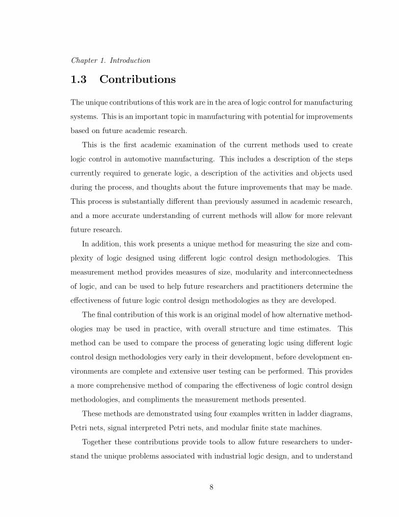
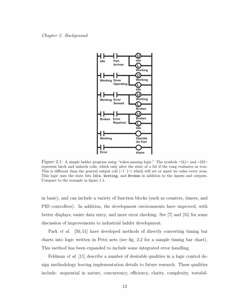
logic” which creates one rung for each transition in the Petri net and used latched
coils to maintain state (see example in fig. 2.1). This is in contrast to ladder diagrams
written by logic designers which generally do not use latched coils, and use one rung
per output. Token-passing logic would defeat the primary debugging methods used
in industry today.
Some companies have begun to implement improvements to the logic design pro-
cess while retaining ladder diagrams. Most modern ladder editors support operations
on integers (such as add, subtract and compare), jump statements (similar to GOTO
12
Chapter 2. Background
Working
Error
U
L
Idle Part
Arrives
L
UWorking Done
Operating
L
UWorking Error
Sensed
L
UBroken Error
Repaired
Idle
Working
Working
Idle
Working
Broken
Broken
Idle
Operate
On Part
Alarm
Figure 2.1: A simple ladder program using “token-passing logic.” The symbols -(L)- and -(U)-represent latch and unlatch coils, which only alter the state of a bit if the rung evaluates as true.This is different than the general output coil (-( )-) which will set or unset its value every scan.This logic uses the state bits Idle, Working, and Broken in addition to the inputs and outputs.Compare to the example in figure 1.1.
in basic), and can include a variety of function blocks (such as counters, timers, and
PID controllers). In addition, the development environments have improved, with
better displays, easier data entry, and more error checking. See [7] and [55] for some
discussion of improvements to industrial ladder development.
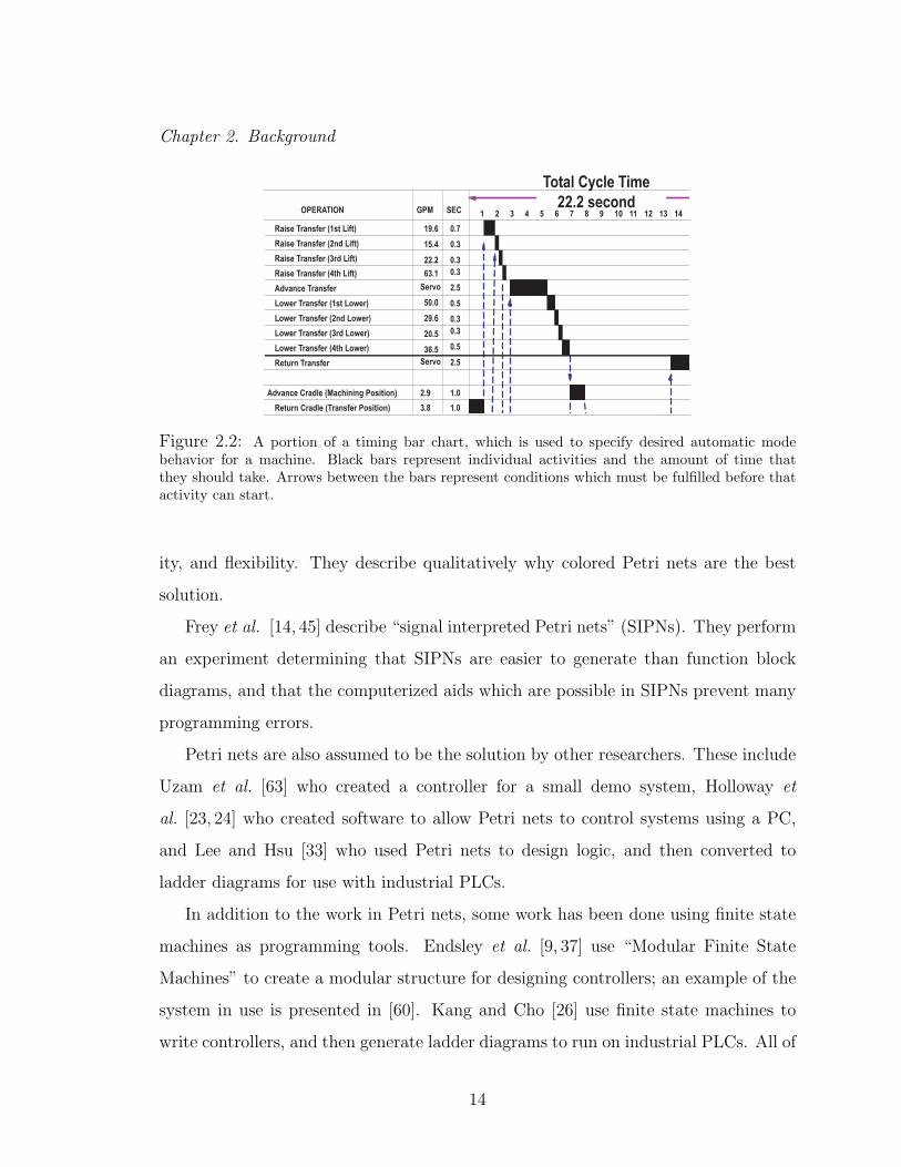
Park et al. [50, 51] have developed methods of directly converting timing bar
charts into logic written in Petri nets (see fig. 2.2 for a sample timing bar chart).
This method has been expanded to include some integrated error handling.
Feldman et al. [11] describe a number of desirable qualities in a logic control de-
sign methodology leaving implementation details to future research. These qualities
include: sequential in nature, concurrency, efficiency, clarity, complexity, testabil-
13
Chapter 2. Background
1 2 3 4 5 6 7 8 9 10 11 12 13 14
Total Cycle Time
22.2 second
0.7
0.3
0.3
0.3
2.5
0.5
0.3
0.3
0.5
2.5
19.6
15.4
22.2
63.1
50.0
Servo
29.6
20.5
36.5
Servo
Return Cradle (Transfer Position)
2.9
3.8
1.0
1.0
Raise Transfer (1st Lift)
Raise Transfer (2nd Lift)
Raise Transfer (3rd Lift)
Raise Transfer (4th Lift)
Advance Transfer
Lower Transfer (1st Lower)
Lower Transfer (2nd Lower)
Lower Transfer (3rd Lower)
Lower Transfer (4th Lower)
Return Transfer
OPERATION GPM SEC
Advance Cradle (Machining Position)
Figure 2.2: A portion of a timing bar chart, which is used to specify desired automatic modebehavior for a machine. Black bars represent individual activities and the amount of time thatthey should take. Arrows between the bars represent conditions which must be fulfilled before thatactivity can start.
ity, and flexibility. They describe qualitatively why colored Petri nets are the best
solution.
Frey et al. [14, 45] describe “signal interpreted Petri nets” (SIPNs). They perform
an experiment determining that SIPNs are easier to generate than function block
diagrams, and that the computerized aids which are possible in SIPNs prevent many
programming errors.
Petri nets are also assumed to be the solution by other researchers. These include
Uzam et al. [63] who created a controller for a small demo system, Holloway et
al. [23, 24] who created software to allow Petri nets to control systems using a PC,
and Lee and Hsu [33] who used Petri nets to design logic, and then converted to
ladder diagrams for use with industrial PLCs.
In addition to the work in Petri nets, some work has been done using finite state
machines as programming tools. Endsley et al. [9, 37] use “Modular Finite State
Machines” to create a modular structure for designing controllers; an example of the
system in use is presented in [60]. Kang and Cho [26] use finite state machines to
write controllers, and then generate ladder diagrams to run on industrial PLCs. All of
14
Chapter 2. Background
this work using finite state machines attempts to create controllers by extending the
supervisory control framework which was begun by Ramadge and Wonham [57, 58,
and related papers].
Other methods that have been considered include C or other computer program-
ming languages [43], Statecharts [22], and flowcharts [48]. All these methods are in
addition to the five languages which are specified in IEC 61131-3 [35].
Except for flowcharts, none of these alternative methodologies have been imple-
mented in industrial scale logic programming.
2.3 Methods of comparison
While there are many opinions regarding the best way to generate industrial control
logic, there are few ways to objectively measure the effectiveness of the various logic
control design methodologies. Many authors have claimed that a particular logic
control design methodology is better than existing methods [1, 11, 16, 22, 37, 45, 50,
51]. These claims are supported with small experiments using novice users (e.g. [45]),
a case study for a particular problem (e.g. [1]), the authors’ intuition (e.g. [22]),
or the presence of certain mathematical properties (e.g. [51]). Some attempts to
quantitatively measure the effectiveness of a logic control design methodology have
been made [34, 38, 65], but the methods of measurement have not yet been validated.
To judge the effectiveness of alternative logic control design methodologies, they
must be compared. Work has been done comparing text-based programming lan-
guages since the 1970’s. This work is discussed in the next section. However, the dif-
ferences between text-based computer programming and the more specialized meth-
ods of creating logic make these results difficult to apply directly. In addition, recent
work has begun comparing logic control design methodologies directly. These efforts
are discussed in section 2.3.2.
15
Chapter 2. Background
2.3.1 Comparisons of Programming Languages
There are a number of ways of comparing traditional, text-based languages. The
most common metric is the number of lines of code (LOC) required to create a
program. A number of more complex measurement methods have risen based on
“software science” [21], which counted the number of operators and operands required,
and how often they are used. Conte et al. [8] discuss many of these methods of
measurement, which typically involved measuring code based on either the number of
lines, operators, operands, functions, modules or similar objects. These measurements
can then be used to estimate size, number of errors, or time required, usually using
empirically derived equations. A typical example is Ss = 102+5.31VARS, where Ss is
the size of the program in lines of code, and VARS is the number of variables required.
These methods have provided insights into how programs are written. However, they
are of limited use when evaluating a new programming language since empirical data
can vary. In addition, it is not clear how they apply to the more graphically based
logic control design methodologies.
In a departure from software science, researchers have begun experimentally ver-
ifying simple hypotheses regarding the behavior of computer programmers.
For example, Gilmore and Green [17] developed the “match-mismatch hypothe-
sis,” which states, “procedural languages would be matched with sequential questions
and declarative languages with circumstantial questions” [17, pg. 31]. Or to general-
ize, the language used should correspond with the type of questions the program will
be used to answer. They tested the comprehension and recall of small programs by
novices and found that the type of information retained was influenced by the method
used to represent the program, either sequential or declarative. The match-mismatch
hypothesis states that the representation used should match the type of information
most often needed by the programmers.
Using this concept to test experienced programmers, Pennington [53, 54] evalu-
ated how well expert Fortan and Cobol programmers were able to study a pre-written
16
Chapter 2. Background
program and answer questions about it. Pennington identified five types of compre-
hension (operation, control flow, data flow, state, function), and determined that the
choice of language affected which types of comprehension were most readily accessible.
It was determined that understanding started at the procedural level, and deepened
as the programmers worked with the code.
More recently, Wiedenbeck et al. [66] performed a test similar to Pennington’s
using C++ and Pascal. They found similar results: from the Pascal representation it
was easier to answer functional questions; from the C++ representation it was easier
to answer control flow and data flow questions.
Bringing this concept to graphical languages, Good [19] performed an experiment
using data flow graphs (resembling FBD) and control flow graphs (resembling flow
charts). Data flow users concentrated more on function and data, while control flow
users concentrated on low level operations.
Others have focused on how to compare different programming languages in a
general way. These methods include creating a list of items to demand from a pro-
gramming languages [67], creating a list of things to consider when comparing pro-
gramming languages [12], or attempting to determine how long a particular piece
of code will take to write [68]. However, methods used for computer programming
languages are hard to directly apply to PLC programming due to differences in the
programming methods and programmers.
All of these studies indicate that the choice of programming language affects the
way that programmers think about the problems that they are solving. However,
none of the studies ever found a definitive “best” language. Thus, it is important not
only to understand the language, but to understand the context in which it is used.
2.3.2 PLC Languages
A few attempts at a more direct comparison of logic control design methodologies
have been made, although these comparisons are all in a restricted domain.
17

Chapter 2. Background
Venkatesh et al. [65] devised a method of comparing the complexity of programs
written using ladders and Petri nets using a “basic element approach.” Their method
was based on counting the number of elements required to represent a particular
program. An “element” was chosen to be a place, transition, or arc for Petri nets or
a contact, coil, rung or branch for ladder diagrams.
A somewhat more sophisticated method of measuring the complexity was pre-
sented by Lee and Hsu [34], which converts the Petri and ladder programs into boolean
expressions, and then counts the number of boolean operators and equations required.
Both of these methods found that Petri nets were smaller, or more compact, than
ladder diagrams.
Frey et al. [15, 16] also describe a quantitative method of measuring the “trans-
parency” of a Petri net based on the structure and comments of the Petri net, although
this method is only effective at comparing Petri nets to each other, not Petri nets to
ladder diagrams or other logic control design methodologies. Independently, Moher
et al. [46] determined that the layout of a Petri net is important to the ability of an
expert to understand its function.
All of these methods of comparison suffer somewhat from the fact that programs
can only be measured after the fact, and the measurement cannot readily be gener-
alized to future programs.
2.4 Task Analysis and GOMS
One thing that is missing from the literature to date is a complete understanding
of the problems associated with logic control for machining systems. For example,
a short survey reveals that the size of Petri nets used in recent academic papers
has been: 64 basic elements [65], 41 rules and operators [34], 63 places [38], and 21
places [63]. Projects observed during this study contained tens of thousands of rungs,
and it is not clear that measurements and intuitions developed using small systems
18

Chapter 2. Background
will work for large systems.
It is difficult to imagine a cost-effective and expedient method of determining the
cost of using a particular logic control design methodology. A first step is to perform
a task analysis [28] to determine what is done using the current system. This should
include everyone affected by the choice of logic control design methodology, including
logic designers, shop floor personnel, and those responsible for making late changes
to the machine behavior. In the future, similar analysis can be done for proposed
methodologies, providing an estimate of cost savings.
GOMS (Goals, Operators, Methods and Selection criteria) is used to model a
human operator’s performance on a given technological system. Olson and Olson [49]
provide an overview of the field.
Early studies focused on very detailed models of relatively simple tasks. For
example, Card et al. [4] experimentally determined the time to perform keystroke-
level operations. Then they demonstrated that this could be used to predict the time
for an expert to perform a task using a predetermined method. This level of analysis
will be used to validate assumptions in section 5.1.1.3. However the keystroke level
of analysis is generally not useful for this study, because different logic control design
methodologies require substantially different higher level constructs.
Later work by Kieras [27, 28] allowed researchers to use a higher level model than
keystrokes. The operators, or lowest level actions, are abstracted to functions the
user must perform, such as “add a module,” independent of the actual user interface
needed to complete the task. This is in contrast to the keystroke level models where
an operator is considered to be an individual keystroke. He suggests that “The
successful design of a system of functionality requires a task analysis early enough in
the system design to enable the developers to create a system that effectively supports
the user’s task.” [28]. Although this level of analysis is less formal than the keystroke
method, it can be used early in the development process of a human-computer system
as a preliminary early predictor of performance. A task analysis is typically used to
19
Chapter 2. Background
analyze or design complex systems of humans and machines, such as maintaining a
subway system [61] or running an air traffic control system [44].
The task analysis methods will be used to describe the structure of logic gener-
ation using the various logic control design methodologies, and provide meaningful
comparisons between them.
2.5 Summary of Logic Control Design Methodolo-
gies Used
As mentioned previously, there are many logic control design methodologies available
for logic control development. The IEC 61131-3 standard includes five languages.
Ladder diagrams are the most common, and will be described below. Sequential
functions charts are a method of controlling the execution of program segments,
and are used in some specific problems. Function block diagrams are a method of
programming using data flow graphs; although they are rarely used now, they are the
basis for the emerging standard 6-1499 [36]. In addition instruction list and structured
text are text based languages, roughly analogous to assembly and C, respectively.
They are rarely used in the U.S. In addition, a nonstandard flow chart language is
used by some developers [48].
In academia, alternative logic control design methodologies have been developed.
Most of these are based on Petri nets, a well known method of analyzing manufac-
turing systems which can be adapted for control. Petri net methods should be easy
to write and debug while allowing some structure. In addition some work has been
done using modular finite state machines. Modular finite state machines should allow
for substantial structure and code reuse.
This work will study programs written using four logic control design methodolo-
gies: ladder diagrams, Petri nets, signal interpreted Petri nets, and modular finite
20

Chapter 2. Background
IR1 Conv1
Part_Trans
IR2 IR2Part_On_1
Conv1
Part_Trans Part_On_2
Figure 2.3: Example of a single rung of a ladder diagram: This is the rung usedto control the Conv1 output. It is equivalent to the boolean expression: Conv1 =((IR1&&Part On 1
) ||Part Trans||Conv1)&&(IR2||Part Trans
)&&
(IR2||Part On 2
). In words,
Conv1 is turned on by either IR1 and NOT Part On 1, or by Part Trans. It is turned off by eitherNOT IR2 and Part Trans or IR2 and Part On 2. This rung comes from an unpublished programwhich uses two conveyors to transport parts, under the constraint that no conveyor ever containstwo parts simultaneously.
state machines. These methods were chosen to compare a reasonable breadth of
academic methodologies as well as the industry standard ladder diagrams. Included
below are details on each of the logic control design methodologies considered in this
dissertation.
2.5.1 Ladder Diagrams
Ladder diagrams are the primary industrial logic control design methodology used in
American industry today. This method is the end result of a gradual evolution from
the physical relays which electricians had previously used to control machining sys-
tems. A ladder diagram consists of individual rungs which are executed sequentially
(see figure 2.3). More details on ladder diagrams can be found in [35].
In general, each rung is the sole control for a single output or internal state
variable. Internal state variables are minimized to preserve “as simple as possible a
path between inputs and outputs” [2]. The program studied in this dissertation (see
chapter 4) was professionally written by and can be found in [62].
21
Chapter 2. Background
IdleC1_Off
C2_ReadyC2_Off
X-ferC1_On
~S2
~S1
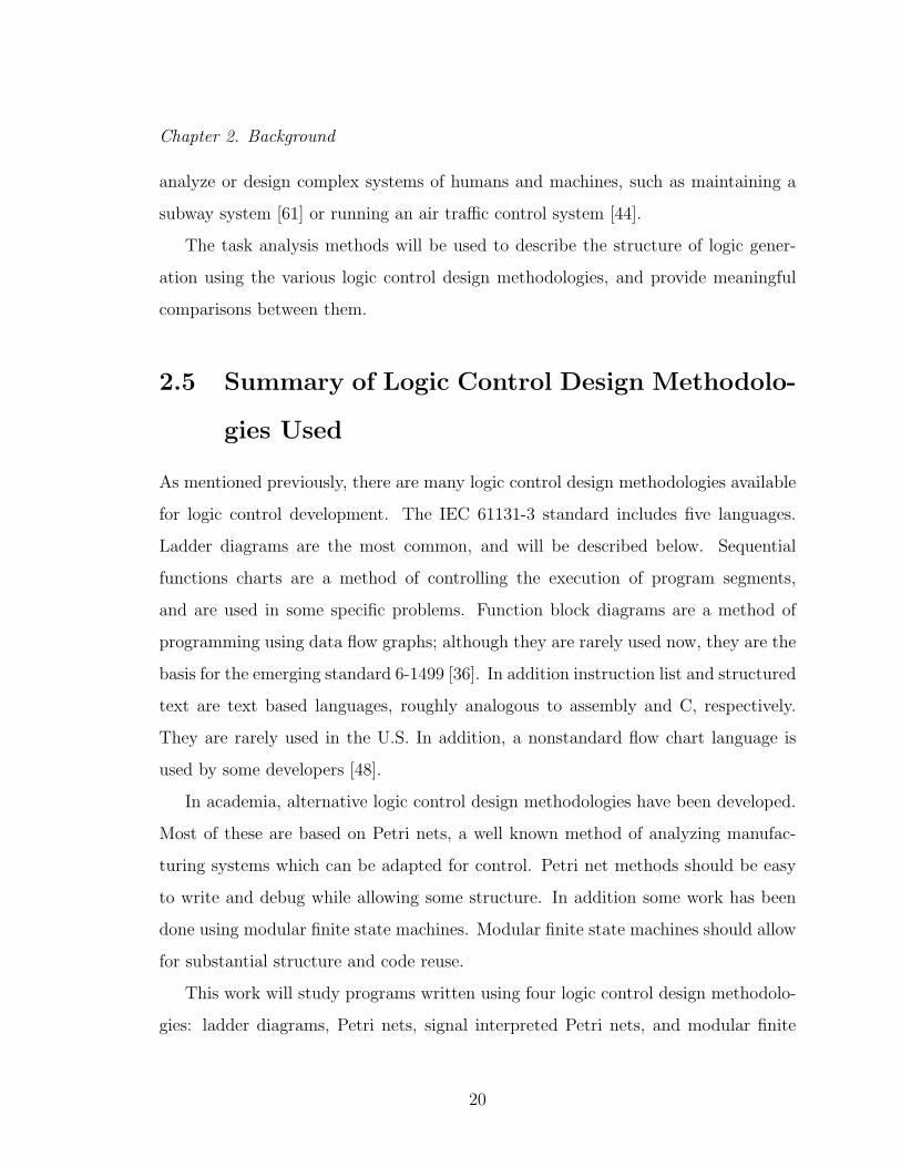
Figure 2.4: Example of a portion of a Petri net. The ovals are called places, and each can hold oneor more tokens, represented by the small dark circles. The places and transitions are connected bydirected arcs, under the restriction that each arc connect a place and a transition. When a transitionfires it removes one token from each place with an arc to the transition, and adds one token to eachplace with an arc from the transition. A transition will fire whenever its condition (usually a sensorvalue, in italics) is true, and firing will not cause any places to have a negative number of tokens.Outputs (in italics) are generated by the places whenever they contain at least one token.
2.5.2 Petri Nets
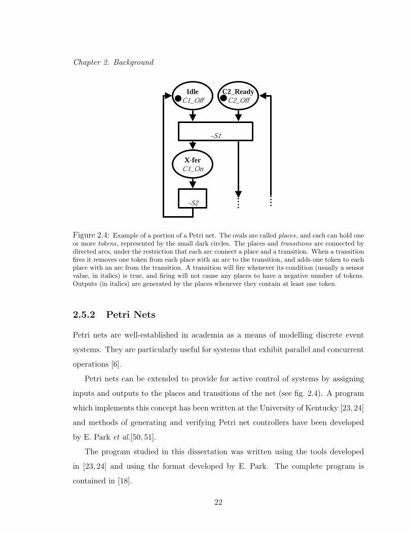
Petri nets are well-established in academia as a means of modelling discrete event
systems. They are particularly useful for systems that exhibit parallel and concurrent
operations [6].
Petri nets can be extended to provide for active control of systems by assigning
inputs and outputs to the places and transitions of the net (see fig. 2.4). A program
which implements this concept has been written at the University of Kentucky [23, 24]
and methods of generating and verifying Petri net controllers have been developed
by E. Park et al.[50, 51].
The program studied in this dissertation was written using the tools developed
in [23, 24] and using the format developed by E. Park. The complete program is
contained in [18].
22

Chapter 2. Background
T3h1
P3h3Move the
Drill Down
T3h3Drill at
Lower Limit
P3h31Wait
T3h31
P3h2Drilling On
4 seconds
True
True
ON Lower Limit Switch
OFF Drill Motor Up
ON Drill Motor Down
OFF Drill Motor Up
OFF Drill Motor Down
OFF Drill Conveyor
ON Drill Spindle
Figure 2.5: Example of a portion of a signal interpreted Petri net. Transitions fire when theirconditions are true, and firing will not cause any transition to have less then zero or more then onetoken. Outputs are generated by combining the output conditions of all active places. Hierarchicalnets are allowed (not shown).
2.5.3 Signal Interpreted Petri Nets
Signal interpreted Petri nets (SIPNs) are a variation on the standard Petri nets frame-
work developed by Frey et al. [14, 45] (see figure 2.5). The primary differences between
SIPNs and standard Petri nets are:
Evolution A transition in SIPN will only fire if there is one token in each in-place,
and there are no tokens in any out-place. Therefore no place will ever contain
multiple tokens. In addition, if the firing of one transition enables another to
fire, the second will fire during the same scan cycle. The absence of racing
conditions resulting from this firing rule can be verified by the development
environment.
I/O A boolean equation on input signals may be placed on a transition as a firing
condition. Each place defines the state for every system output as either 0 (off),
1 (on), or − (don’t care). The actual output is the sum of the outputs of each
23

Chapter 2. Background
place which contains a token. The development environment ensures that the
output is fully defined and not contradictory.
Hierarchy SIPNs allow hierarchy. A subnet may be placed within a single place of
a Petri net. Conditions are defined in [14] to ensure deterministic behavior.
The program used in this dissertation (see chapter 4) was developed by Stephane
Klein [31]. The complete program is shown in [30].
Additional variants on Petri nets are occasionally used in literature. For example,
Uzam et al.[63] use Petri nets with inhibitor arcs to control a model system. They
use reachability graphs to validate the system, and then generate ladder diagrams
via “token-passing logic.” Peng and Zhou [52] survey the state of research regarding
conversion between Petri nets and ladder diagrams, and generally find conversion
schemes lacking.
2.5.4 Modular Finite State Machines
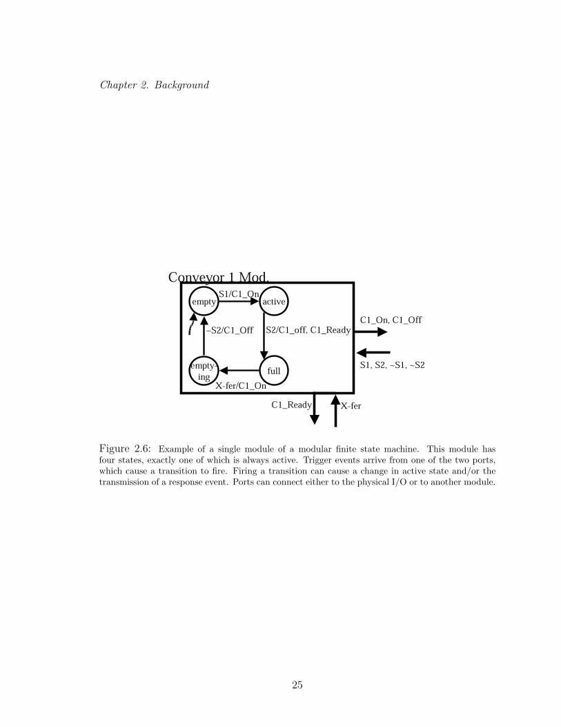
Modular finite state machines are an extension of the standard finite state machine
formulation. A modular finite state machine program consists of a set of modules,
each of which contains a trigger/response finite state machine, and instructions for
communicating with other modules. This method attempts to preserve the formality
and verifiability for finite state machines in a modular framework (see fig. 2.6). Details
can be found in [37].
The program studied in this dissertation was created using the software tools
developed in [9]. A report on this coding effort is in [60].
24
Chapter 2. Background
empty active
fullempty-
ing
S1/C1_On
S2/C1_off, C1_Ready
X-fer/C1_On
~S2/C1_Off
C1_Ready X-fer
C1_On, C1_Off
S1, S2, ~S1, ~S2
Conveyor 1 Mod.
Figure 2.6: Example of a single module of a modular finite state machine. This module hasfour states, exactly one of which is always active. Trigger events arrive from one of the two ports,which cause a transition to fire. Firing a transition can cause a change in active state and/or thetransmission of a response event. Ports can connect either to the physical I/O or to another module.
25

Chapter 3
The Current Logic Design Process
The primary contribution of this chapter is a comprehensive understanding of the
current logic design methods used in industry. This was accomplished through an
observational study of logic designers at Lamb Technicon. A paper based on the
work presented in chapter has been accepted for publication in the International
Journal of Human-Computer Studies [42].
3.1 Study Methods
From September to December of 2001, observations were made at Lamb for approx-
imately 110 hours on 28 different days. During this time, portions of three projects
in three different stages of development were observed.
The primary project observed was in the middle of the development cycle. Both
a team leader and a team member were observed during the study. Most of the
team leader’s time was spent coordinating the project among the team members, as
well as entering logic from the previous project, and managing the memory map (see
table 3.2). The team member was responsible for implementing a more advanced
part tracking scheme than was usual, and therefore spent much of his time creating
new logic (see table 3.3). A portion of this ladder logic maintained a database with
26

Chapter 3. The Current Logic Design Process
approximately 10,000 entries, updating and reading information about the current
status of parts in the system.
Another project observed was in the “Installation and Debugging” stage (see fig-
ure 3.2). This project consisted of three machines with roughly 20 stations and
between 2 and 4 transfer bars per machine. Developers estimated the size of logic
required for a single machine at 3000 + 1500n rungs, where n equals the number of
stations in the machine (about 100,000 for the entire project). These machines con-
tained the minimal level of diagnostic logic possible, so presumably another machine
could contain more logic.
The final project observed was only observed over two days, once during the
project planning stage, and once near the beginning of the development stage.
The three projects were developed using three different development environments
(RSLogix, FrameworX, and Omron respectively). These environments were incom-
patible, in that data from one could not be transferred to any other.
The logic developers observed were all very experienced. Everyone observed had
at least 12 years experience, and the team leaders had at least 20. Some employees
in smaller roles had less experience, and they were more closely supervised. Most
developers had no formal post-secondary education.
During this time approximately 130 pages of notes were taken by hand. The notes
included a summary of the activities performed broken down into ten minute intervals,
as well as descriptions of subtasks used to complete a single task when possible, and
any other relevant observations. Data taken during the cycle and debug stage was
taken in 20 minute intervals, due to the less structured nature of the task.
After the observations were complete, each description of subtasks was separated
from the notes and typed up. Similar tasks were grouped into categories. Using this
method the following activity categories were developed: Project coordination and
planning, File creation and maintenance, Memory management, Copy/Modify logic
entry, New logic development, and Debugging (see table 3.1 for details).
27

Chapter 3. The Current Logic Design Process
ProjectSpecific
Specifications
KnownStandardSpecifications
ControlLogic
LogicDesigner
ABCZ
%I36%I37%I38%O59
A
C
ZB
Specs
UnspecifiedRequirements
Figure 3.1: Overview of the logic generation process: Logic Designers are given control specifi-cations and machine schematics to describe the logic needed. These are combined with standardspecifications (usually in the form of a previous project) to create the needed control logic. Unspec-ified requirements can include late changes or unexpected constraints in the machine or electronics.
Once the activity categories were developed, the time-based data was examined.
Each 10 minute portion of time was categorized into either one of the six project
related activities, or an additional non-project related task. If multiple activities
were recorded in the ten minute section of time, the primary activity was recorded.
This data is summarized in tables 3.2, 3.3, and 3.4.
3.2 Study Results
3.2.1 Overview of Logic Development Process
A simple description of the approach used to create control logic is shown in figure 3.1.
The logic designers are given project specific specifications and schematics. Using an
28
Chapter 3. The Current Logic Design Process
Controls Lineup
Pro
jec
t P
lan
nin
g
Copy/Modify
HMI Development
New CodeDevelopment
Ins
tall
ati
on
&
Deb
ug
gin
g
Re
as
sa
mb
le/T
es
t
Dis
as
sa
mb
le/S
hip
Customer Shakedown
1 Day
1 Week
4 Months
1 Month
3-4 Days
1 Month
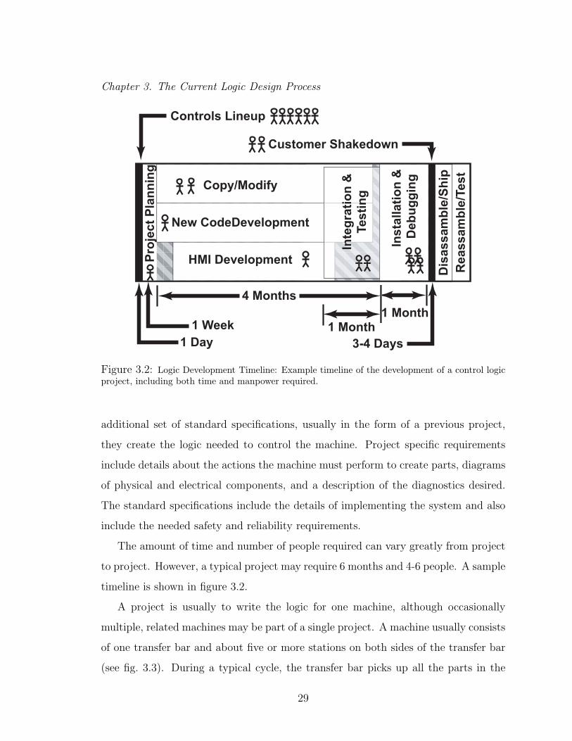
Figure 3.2: Logic Development Timeline: Example timeline of the development of a control logicproject, including both time and manpower required.
additional set of standard specifications, usually in the form of a previous project,
they create the logic needed to control the machine. Project specific requirements
include details about the actions the machine must perform to create parts, diagrams
of physical and electrical components, and a description of the diagnostics desired.
The standard specifications include the details of implementing the system and also
include the needed safety and reliability requirements.
The amount of time and number of people required can vary greatly from project
to project. However, a typical project may require 6 months and 4-6 people. A sample
timeline is shown in figure 3.2.
A project is usually to write the logic for one machine, although occasionally
multiple, related machines may be part of a single project. A machine usually consists
of one transfer bar and about five or more stations on both sides of the transfer bar
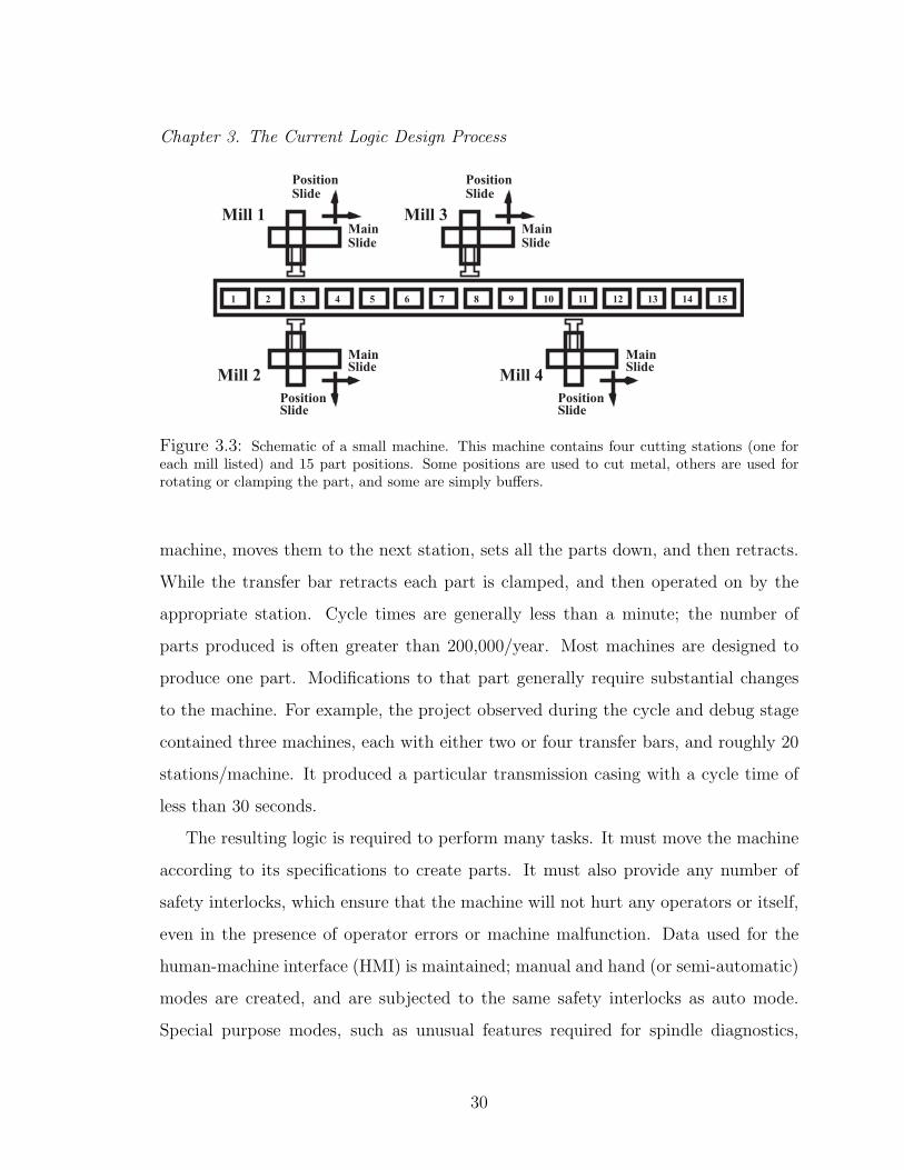
(see fig. 3.3). During a typical cycle, the transfer bar picks up all the parts in the
29
Chapter 3. The Current Logic Design Process
Position
Slide
Main
Slide
Position
Slide
Main
Slide
Position
Slide
Main
Slide
Position
Slide
Main
Slide
1 2 3 4 5 6 7 8 9 10 11 12 13 14 15
Mill 1
Mill 2
Mill 3
Mill 4
Figure 3.3: Schematic of a small machine. This machine contains four cutting stations (one foreach mill listed) and 15 part positions. Some positions are used to cut metal, others are used forrotating or clamping the part, and some are simply buffers.
machine, moves them to the next station, sets all the parts down, and then retracts.
While the transfer bar retracts each part is clamped, and then operated on by the
appropriate station. Cycle times are generally less than a minute; the number of
parts produced is often greater than 200,000/year. Most machines are designed to
produce one part. Modifications to that part generally require substantial changes
to the machine. For example, the project observed during the cycle and debug stage
contained three machines, each with either two or four transfer bars, and roughly 20
stations/machine. It produced a particular transmission casing with a cycle time of
less than 30 seconds.
The resulting logic is required to perform many tasks. It must move the machine
according to its specifications to create parts. It must also provide any number of
safety interlocks, which ensure that the machine will not hurt any operators or itself,
even in the presence of operator errors or machine malfunction. Data used for the
human-machine interface (HMI) is maintained; manual and hand (or semi-automatic)
modes are created, and are subjected to the same safety interlocks as auto mode.
Special purpose modes, such as unusual features required for spindle diagnostics,
30

Chapter 3. The Current Logic Design Process
Table 3.1: Categorization of activities performed
Project Coordination
and Planning
Coordinating between the various people working on a
project, planning for a project, or creating documentation
for the project. Most coordination is to ensure consistent
communications between various processors in the system.
File Creation and
Maintenance
Creating new files, performing version control and similar
activities.
Memory Manage-
ment
Creating or modifying the manually allocated memory
space of the project.
Copy/Modify Entering logic by copying from another source. This can
be either from a previous project, or from other portions of
the current project. This usually includes making minor
modifications, such as changing the names on the rungs.
New Development Creating new logic. This is usually done for features which
were not present on the previous machine.
Debugging Testing existing logic and making any changes necessary.
are added. Finally any data required for diagnostic messages must be created and
maintained. The logic to create the automatic mode is generally reported to be about
10% of the total.
3.2.2 Activities observed
There are several separate activities that are needed to successfully generate industrial
logic. While observing the logic designers, most of their activities could be divided
into six basic categories: project coordination and documentation, creating and man-
aging files, memory management, copy/modify, new development, and debugging (see
31

Chapter 3. The Current Logic Design Process
table 3.1). There is no separate category for top-level design, as would be expected in
a software development team. Since most of the logic is taken from a previous project,
much of the top level design is implied from the start. The rest occurs within the con-
text of either project coordination (e.g. supervisors telling engineers how the project
should look in the end), or memory management (e.g. allocating certain blocks of
memory to certain people and functions, thereby implying a certain data structure).
A more detailed description of these activities is included in sections 3.2.2.1–3.2.2.6.
There were other activities observed which did not directly relate to the process
of generating logic. These included a variety of planned meetings to discuss com-
pany standards, project status or other coordination needs. In addition there were
demonstrations, new project quotations, filling out timesheets etc. It is unlikely that
all activities were observed in this study, but we believe that most of the activities
needed to generate the logic were.
A tabulation of time spent in the various activities can be found in tables 3.2, 3.3,
and 3.4. The data was broken into three different tables so that the differences
between design stages could be seen. In addition, observation times were not chosen
randomly, so a total tabulation would not be an accurate reflection of the activities
needed.
Most of these numbers are not particularly surprising. It is interesting to note how
much time the team leaders spend coordinating with their team members. This co-
ordination is mostly discussing and confirming the communication protocols between
the various processors needed to make the machine run. For example, in the primary
project observed, the main PLC logic interfaced with separate CNC processors which
controlled the machine. A lot of time was spent ensuring that the communication
between the different processors was consistent.
A detailed description of the activities is below.
32

Chapter 3. The Current Logic Design Process
Table 3.2: Tabulation of data from project team leaders. Time spent in planned meetings was notconsidered.
Minutes Percent of
Activity Observed project time
Project Coordination 920 44 %
New Development 130 6 %
Copy/Modify 450 22 %
Memory Management 310 15 %
File Maintenance 70 3 %
Debugging 200 10 %
GUI Development 0 0 %
Talking to data taker 320 N/A
Break (lunch etc) 370 N/A
Other 320 N/A
3.2.2.1 Project Coordination and Documentation
Project coordination and documentation describes a broad range of activities nec-
essary to coordinate the developers on a project. While this includes writing some
documentation, most of this time is spent coordinating the efforts of other team
members. Project coordination and documentation is the most important activity of
project team leaders (see table 3.2).
A description of the documentation produced is described in section 3.2.3.7. Pro-
ducing documentation does not take a significant amount of time. When modifying
an existing portion of the documentation the designer will generally confirm relevant
portions, updating any information which was recently changed. When creating new
portions of documentation, the relevant information is entered either by hand (e.g.
for the change log) or via copy/paste (e.g. for the memory map).
Since the teams of logic designers were relatively small (about 4-6 people) most of
33
Chapter 3. The Current Logic Design Process
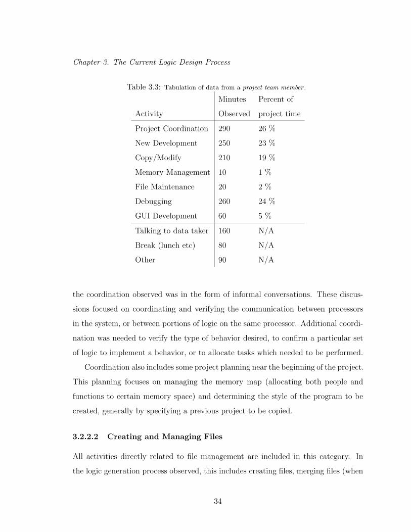
Table 3.3: Tabulation of data from a project team member .
Minutes Percent of
Activity Observed project time
Project Coordination 290 26 %
New Development 250 23 %
Copy/Modify 210 19 %
Memory Management 10 1 %
File Maintenance 20 2 %
Debugging 260 24 %
GUI Development 60 5 %
Talking to data taker 160 N/A
Break (lunch etc) 80 N/A
Other 90 N/A
the coordination observed was in the form of informal conversations. These discus-
sions focused on coordinating and verifying the communication between processors
in the system, or between portions of logic on the same processor. Additional coordi-
nation was needed to verify the type of behavior desired, to confirm a particular set
of logic to implement a behavior, or to allocate tasks which needed to be performed.
Coordination also includes some project planning near the beginning of the project.
This planning focuses on managing the memory map (allocating both people and
functions to certain memory space) and determining the style of the program to be
created, generally by specifying a previous project to be copied.
3.2.2.2 Creating and Managing Files
All activities directly related to file management are included in this category. In
the logic generation process observed, this includes creating files, merging files (when
34
Chapter 3. The Current Logic Design Process
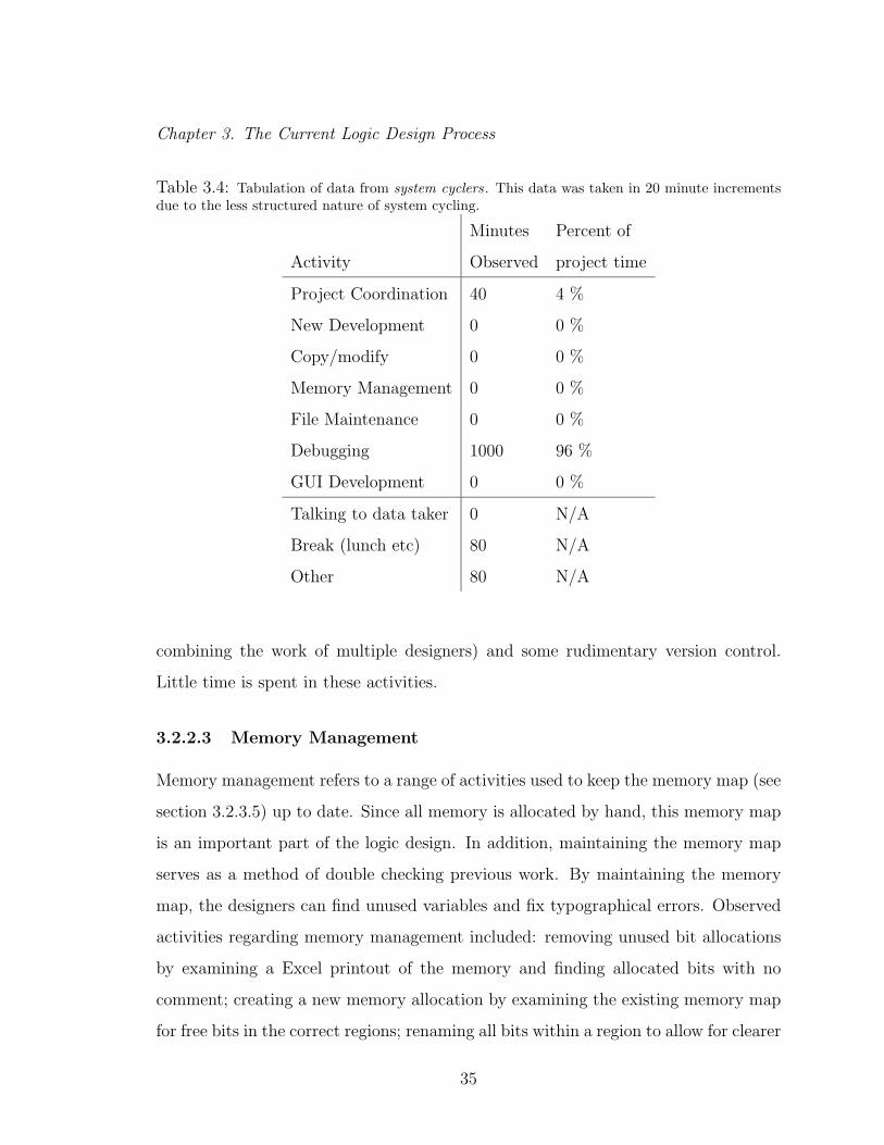
Table 3.4: Tabulation of data from system cyclers. This data was taken in 20 minute incrementsdue to the less structured nature of system cycling.
Minutes Percent of
Activity Observed project time
Project Coordination 40 4 %
New Development 0 0 %
Copy/modify 0 0 %
Memory Management 0 0 %
File Maintenance 0 0 %
Debugging 1000 96 %
GUI Development 0 0 %
Talking to data taker 0 N/A
Break (lunch etc) 80 N/A
Other 80 N/A
combining the work of multiple designers) and some rudimentary version control.
Little time is spent in these activities.
3.2.2.3 Memory Management
Memory management refers to a range of activities used to keep the memory map (see
section 3.2.3.5) up to date. Since all memory is allocated by hand, this memory map
is an important part of the logic design. In addition, maintaining the memory map
serves as a method of double checking previous work. By maintaining the memory
map, the designers can find unused variables and fix typographical errors. Observed
activities regarding memory management included: removing unused bit allocations
by examining a Excel printout of the memory and finding allocated bits with no
comment; creating a new memory allocation by examining the existing memory map
for free bits in the correct regions; renaming all bits within a region to allow for clearer
35

Chapter 3. The Current Logic Design Process
documentation; allocating portions of memory to different team members to allow
for parallel development; and searching for a particular bit comment by scanning an
Excel printout. Excel is used for memory management because of the poor usability
properties of the development environments.
Some development environments require that all memory is allocated and man-
aged based on its physical location. This means that to reference a particular bit
the designer must know exactly where the bit is located physically, for example
“135:04” would mean the 135th word addressed by the current processor, the 4th
bit in that word. Some recent development environments allow memory addresses
to be named. However, such features do not appear to be widely used, even when
they exist. The main project observed used such a system. At the beginning of
the project, the designer attempted to use named memory, for example creating a
bit named Station 12 tool fault. However, all his previous experience was using
numbered memory, the development environment enforced a 15 character limit on
names, and managing thousands of global variable names quickly became unwieldy.
He then renamed all variables to reflect their physical location.
3.2.2.4 Copy/Modify
Copy/Modify is the process of entering logic which has already been designed. This is
usually done by copying from either a previous project or a previously written portion
of the same project. Most rungs need minor modification (for example changing the
references to the memory map, or adjusting the number of safety conditions enforced).
The steps to generating logic in this manner generally follow the following sequence:
1) create a blank rung, 2) create the correct (known) pattern of contacts on that
rung, 3) create a coil on the rung, 4) enter the correct bit name for each contact or
coil. The correct bit name is often known to the designer, and can be typed in. Other
methods to name a contact or coil are: to drag the name from another rung onto the
correct place on the current rung; to search the variable list manually, either within
36
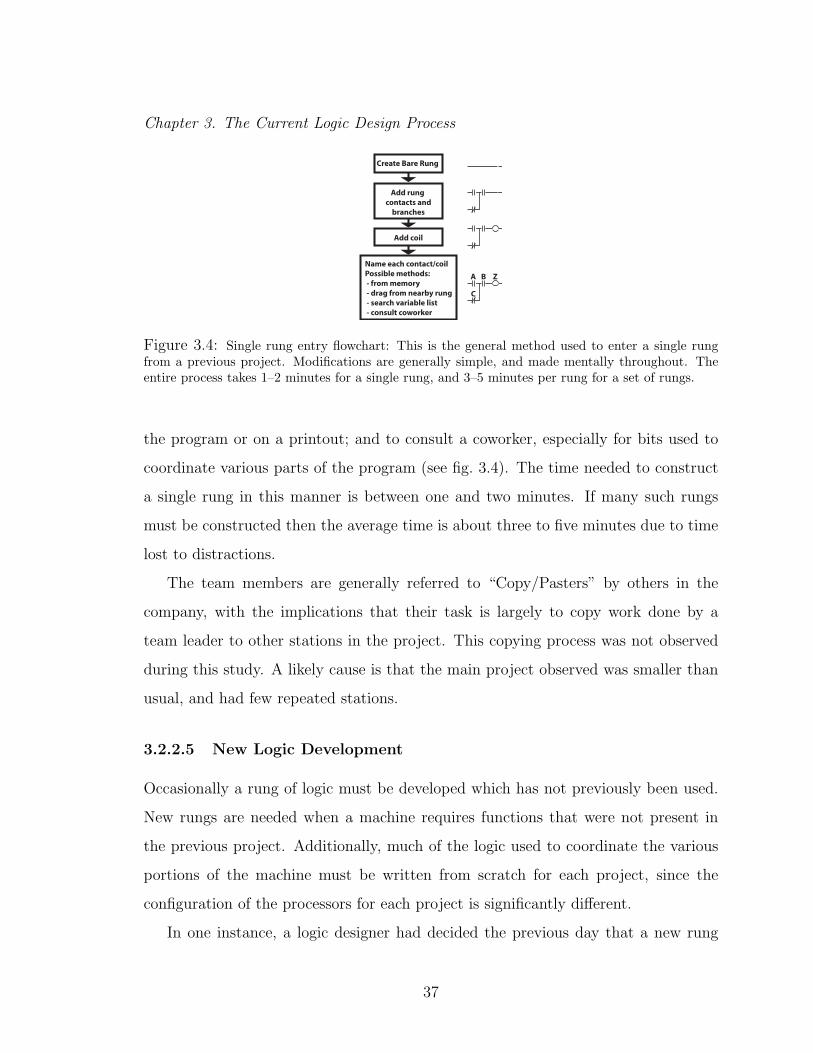
Chapter 3. The Current Logic Design Process
Create Bare Rung
Add rung contacts and
branches
Add coil
Name each contact/coilPossible methods: - from memory - drag from nearby rung - search variable list - consult coworker
A
C
ZB
Figure 3.4: Single rung entry flowchart: This is the general method used to enter a single rungfrom a previous project. Modifications are generally simple, and made mentally throughout. Theentire process takes 1–2 minutes for a single rung, and 3–5 minutes per rung for a set of rungs.
the program or on a printout; and to consult a coworker, especially for bits used to
coordinate various parts of the program (see fig. 3.4). The time needed to construct
a single rung in this manner is between one and two minutes. If many such rungs
must be constructed then the average time is about three to five minutes due to time
lost to distractions.
The team members are generally referred to “Copy/Pasters” by others in the
company, with the implications that their task is largely to copy work done by a
team leader to other stations in the project. This copying process was not observed
during this study. A likely cause is that the main project observed was smaller than
usual, and had few repeated stations.
3.2.2.5 New Logic Development
Occasionally a rung of logic must be developed which has not previously been used.
New rungs are needed when a machine requires functions that were not present in
the previous project. Additionally, much of the logic used to coordinate the various
portions of the machine must be written from scratch for each project, since the
configuration of the processors for each project is significantly different.
In one instance, a logic designer had decided the previous day that a new rung
37

Chapter 3. The Current Logic Design Process
Consider:-Purpose of output-Inputs-Safety considerations
Create Initial Rung
Think ofChange
Mentally Simulate
Rung
Make Change in(structure or memory)
No Error
Error
25%
75%
A
C
Z
A
C
ZB
Figure 3.5: New rung development flowchart: This is the general method used when generatingnew rungs of logic. The “Create Initial Rung” step is equivalent to the flowchart shown in figure 3.4.
was required, and appeared to have put substantial thought into it before arriving at
work. In this case entering this rung was much like “Copy/Modify” in section 3.2.2.4.
The primary difference was that the process was slower, and the contact pattern was
changed after the process had begun. Additionally, after entering the rung there was
a verification step, including an examination of the rung, and examination of the
memory map for any relevant bits which were not present in the rung (see fig. 3.5).
In other cases of developing new rungs, the process was not well defined, and much
of the work was purely cognitive and not observed. The process generally started with
a specification of some kind for the rungs to be developed. Written specifications ob-
served were timing bar charts (describing the desired communication between two
portions of the controller), a state machine (describing the desired behavior of the
machine during an error recovery), and purely verbal descriptions. Observable activi-
ties included scribbling on paper and “drawing” in the air with his finger, apparently
visualizing the rung of logic. Once a candidate rung had been designed, it was ver-
ified by drawing it, and checking every “path” (i.e. OR branch) through the rung
against whatever specifications had been provided. Verifying the candidate against
the specification was not a simple activity, since all the specifications were sequential
in nature, and ladder diagrams are functional in nature.
38
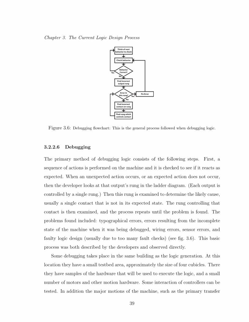
Chapter 3. The Current Logic Design Process
Think of nextbehavior to check
BehaviorCorrect?Yes
Check behavior
Find incorrectoutput rung
Find incorrectcontact on rung
Error inthis rung?
Find rung whichcontrols contact
Fix Error
No
Yes
No
Figure 3.6: Debugging flowchart: This is the general process followed when debugging logic.
3.2.2.6 Debugging
The primary method of debugging logic consists of the following steps. First, a
sequence of actions is performed on the machine and it is checked to see if it reacts as
expected. When an unexpected action occurs, or an expected action does not occur,
then the developer looks at that output’s rung in the ladder diagram. (Each output is
controlled by a single rung.) Then this rung is examined to determine the likely cause,
usually a single contact that is not in its expected state. The rung controlling that
contact is then examined, and the process repeats until the problem is found. The
problems found included: typographical errors, errors resulting from the incomplete
state of the machine when it was being debugged, wiring errors, sensor errors, and
faulty logic design (usually due to too many fault checks) (see fig. 3.6). This basic
process was both described by the developers and observed directly.
Some debugging takes place in the same building as the logic generation. At this
location they have a small testbed area, approximately the size of four cubicles. There
they have samples of the hardware that will be used to execute the logic, and a small
number of motors and other motion hardware. Some interaction of controllers can be
tested. In addition the major motions of the machine, such as the primary transfer
39
Chapter 3. The Current Logic Design Process
bar, can be tested.
Most debugging takes place while the machine is being assembled. This is referred
to as “cycling” the machine. During this process the logic is installed and portions
are “jumpered out”, i.e. circumvented using temporary contacts in the rungs. (For
example the portions dealing with safety gates are jumpered out during the time
before the safety gates are installed.) The incomplete logic is used to validate both
the correct construction of the machine and the correct operation of the logic.
Errors observed during this stage included: improper part handling, inconsistent
operation of the machine, safety gates that would not open, and incorrect displays on
the user interface. These problems were caused by: wiring errors, faulty conditions
in the logic, misplaced sensors, and the incomplete state of the machine while it was
being debugged. Cyclers seemed comfortable debugging errors caused by any of these
conditions.
Since the installation and debugging takes place while the machine is being built,
there are frequent interruptions. Interruptions observed included: accidentally pulling
an emergency stop cord, hydraulic leaks, waiting for the assemblers to be clear of the
moving parts, and phone calls. In addition, due to the size of the machine (about 50
meters long), it took considerable walking time when another developer needed to be
consulted. Walkie-talkie’s were used occasionally, but they didn’t always work well
due to the background noise and static generated by the machine.
In-house debugging is done as needed during the development, and does not take
a significant amount of time. Cycling the machine took about one month, or about
20% of the development time.
3.2.3 Objects used when Developing Logic
In addition to the types of activities, it is important to understand the tools and
documents used through the development process. The primary objects used are
described below. Their relationship to the activities described in section 3.2.2 is
40
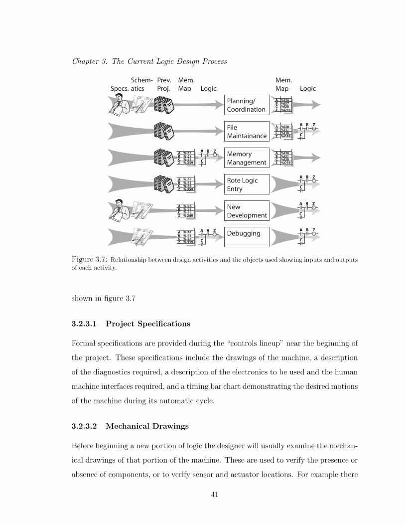
Chapter 3. The Current Logic Design Process
NewDevelopment
Debugging
Rote LogicEntry
FileMaintainance
MemoryManagement
Planning/Coordination
A
CC
ZB
A
CC
ZB
A
CC
ZB
A
C
ZBABCZ
%I36%I37%I38%O59
ABCZ
%I36%I37%I38%O59
ABCZ
%I36%I37%I38%O59
A
C
ZZB
A ZZB
ABCZ
%I36%I37%I38%O59
ABCZ
%I36%I37%I38%O59
ABCZ
%I36%I37%I38%O59
ABCZ
%I36%I37%I36%O59
SpecsSpecs
LogicLogicMem.MapSpecs.
Schem-atics
Mem.Map
Prev.Proj.
Figure 3.7: Relationship between design activities and the objects used showing inputs and outputsof each activity.
shown in figure 3.7
3.2.3.1 Project Specifications
Formal specifications are provided during the “controls lineup” near the beginning of
the project. These specifications include the drawings of the machine, a description
of the diagnostics required, a description of the electronics to be used and the human
machine interfaces required, and a timing bar chart demonstrating the desired motions
of the machine during its automatic cycle.
3.2.3.2 Mechanical Drawings
Before beginning a new portion of logic the designer will usually examine the mechan-
ical drawings of that portion of the machine. These are used to verify the presence or
absence of components, or to verify sensor and actuator locations. For example there
41
Chapter 3. The Current Logic Design Process
is occasionally an important distinction made between stations with services on the
left or on the right due to the location of multiple processors and a desire to minimize
wiring.
3.2.3.3 Electrical Drawings
All the designers observed were proficient at reading electrical drawings for the ma-
chine. These were consulted both during the design phase, to ensure that electrical
components were properly interfaced, and during the debugging stage, since it is often
difficult to tell a logic error from a wiring error.
3.2.3.4 Printout of previous project
When a project is started a previous project is found which is similar (especially in
terms of amount of memory). A large part of creating logic for a new project is copying
logic from the previous project into the new one. In most cases this means the same
logic, manipulating the same memory locations for the same purpose. This helps to
ensure that bugs which have been fixed in the previous project are not recreated in
the current project.
Logic and memory maps must be re-entered by hand since all development envi-
ronments are assumed to be incompatible, including different versions from the same
vendor.
3.2.3.5 The Memory Map
A part of the generated logic is the map of all memory in the system. Included in this
map is its physical address, its tag (i.e. name), a comment regarding its meaning, its
initial value, whether or not it is retentive (i.e. will be stored upon loss of power),
and occasionally other information. The memory map is actively maintained by hand,
and by looking at the memory map the designers can double check portions of their
logic.
42
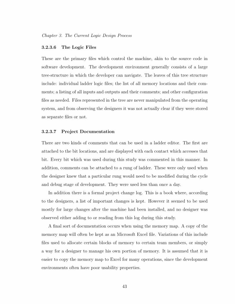
Chapter 3. The Current Logic Design Process
3.2.3.6 The Logic Files
These are the primary files which control the machine, akin to the source code in
software development. The development environment generally consists of a large
tree-structure in which the developer can navigate. The leaves of this tree structure
include: individual ladder logic files; the list of all memory locations and their com-
ments; a listing of all inputs and outputs and their comments; and other configuration
files as needed. Files represented in the tree are never manipulated from the operating
system, and from observing the designers it was not actually clear if they were stored
as separate files or not.
3.2.3.7 Project Documentation
There are two kinds of comments that can be used in a ladder editor. The first are
attached to the bit locations, and are displayed with each contact which accesses that
bit. Every bit which was used during this study was commented in this manner. In
addition, comments can be attached to a rung of ladder. These were only used when
the designer knew that a particular rung would need to be modified during the cycle
and debug stage of development. They were used less than once a day.
In addition there is a formal project change log. This is a book where, according
to the designers, a list of important changes is kept. However it seemed to be used
mostly for large changes after the machine had been installed, and no designer was
observed either adding to or reading from this log during this study.
A final sort of documentation occurs when using the memory map. A copy of the
memory map will often be kept as an Microsoft Excel file. Variations of this include
files used to allocate certain blocks of memory to certain team members, or simply
a way for a designer to manage his own portion of memory. It is assumed that it is
easier to copy the memory map to Excel for many operations, since the development
environments often have poor usability properties.
43
Chapter 3. The Current Logic Design Process
44%
ProjectCoordination
Mem.Manage-Manage-
ment15%
Other
13%28%
Installation andDebugging Begins
Project Planning Complete
Copy/Paste
Think of nextoutput to control
RungAlready Exists?
Electronic or Paper?
Create Rung structure
Modify if neededAssociate
contacts/coilswith memory map
Consider:-Purpose of output-Inputs-Safety considerations
Create Rung
Think ofChange
Check rung
Mentally Simulate
Rung
FixErrors
Make Change(structure, memory)
MoreOutputsNeeded?
NoYes
PaperElectronic
No Error
Error
No Error
Error
No
Yes
25% 75%
25%
75%
50%
4
2
1
1
0.5
4
0.5
1
1
2
0.5
50%
5%95%
Typical Process of Generating Logic
Includes:-Instructing Employees-Defining inter-processor communication-Creating Documentation
Includes:-Defining memory
(Which defines algorithm)-Validating memory forconsistancy
Includes:-File maintenance-Updating previous projects-Some debugging
Figure 3.8: Logic Development Flowchart: Flowchart describing the tasks required of the logicdesign team leader during a logic design project. Numbers within the block represent an approximateestimate (in minutes) of the time to complete a task. Using the numbers in the figure, a rung oflogic will average about 16 minutes of “Logic Generation” time. Considering that logic generationtime accounts for 28% of total time, a project which requires the lead programmer to develop 3000rungs should take take about 5 months. This is close to the observed time (listed as four months infigure 3.2).
3.2.4 Summary of Results
A summary of the logic development process used by the logic design team leader is
shown in figure 3.8. During this time approximately one quarter of his time is spent
44
Chapter 3. The Current Logic Design Process
actually generating logic for the controller. Approximate times for each sub-step of
this process are listed in the figure. For a project requiring 3000 rungs from the team
leader, this process will take approximately five months, close to the observed time
of four months shown in figure 3.2. Of course all times and numbers in a study like
this have a large margin for error.
3.3 Improving Logic Design
There are a variety of ways that the results of this study can be used to improve
methodologies proposed for logic control development or development environments
used within a particular methodology.
3.3.1 Improvements within Ladder Diagrams
3.3.1.1 Time Consuming Activities
As a first step towards improvement, the process can be examined for activities which
consume inordinate amounts of time, or activities which could be eliminated with
proper computer assistance.
In the projects studied, a lot of time was spent in the broad category of planning
and coordination. (See section 3.2.2.1.) It may be possible for this process to be more
efficient. Possibilities for reducing the amount of time required for project coordina-
tion may be managerial, perhaps more formalized specification development or more
coordination at earlier stages of design. They may also be technical, for example
higher level logic control design methodologies, methodologies which perform some
coordination automatically, or methodologies which enforce modular logic develop-
ment. However, this study does not provide an obvious direction for improvements
in this area.
An additional time consuming step is the process described as copy/modify. (See
45
Chapter 3. The Current Logic Design Process
section 3.2.2.4.) In this process logic must be retyped from previously written logic.
One of the unique skills observed in one of the team members was intelligent copy/
paste/renaming. Once, when entering a large number of similar rungs, significant
effort was applied to ensuring that the variable names chosen could all be modified to
the proper values using the automated “replace” tools provided with the development
environment. Using these methods, he was able to enter a series of 24 rungs, with
25 items per rung, in about 1 hour 15 minutes (an average of eight items/minute).
While his skill at intelligently choosing replace values was useful, the entire operation
could have been accomplished with one nested FOR loop (about 15 lines) in a language
like C. When copying code from a previous project, it may be more efficient if it were
possible to use copy/paste features, rather than re-entering every rung. However, this
is not currently possible due to compatibility issues.
A final time consuming operation is the maintenance of the memory map. (See
section 3.2.2.3.) This is somewhat time consuming (about 15% of the team leader’s
time) and seems to manage entirely redundant information. However, memory man-
agement serves as a focus in organizing operations. A significant activity observed
during a particular project planning operation was allocating the memory map. This
involved a top-level memory map which listed sections of memory, what data was
going to be stored in that memory, the functions supported by that data, and the
person responsible for writing the logic which maintains that data. This provides
the focus for a database-first design strategy, and eliminating the step entirely would
force designers to devise entirely new methods of project planning.
However, in the two development environments in which memory management
was observed it was considered easier to do all memory maintenance tasks in Mi-
crosoft Excel, rather than within the development environment. While the seemingly
redundant activity may provide unexpected value, improvements can still be made
within the development environment.
The other activities listed in section 3.2.2 (file maintenance, new development and
46
Chapter 3. The Current Logic Design Process
debugging) are not included here since they seem to involve fundamental, irreducible
activities when developing logic using ladder diagrams.
3.3.1.2 Improving the Development Environment
The usability of the development environments is lower than would be expected of
commercial software. For example, at one point a team member was told to enter a
list of error messages from an Excel spreadsheet into the development environment.
Each message had to be entered and associated with an address. For each of the 100
or so messages the employee needed to fill out a multi field dialog box, so the message
had to be retyped, the address retyped, and about four mouse clicks were needed.
What could have been a quick copy/paste operation took more than an hour.
There were other examples of problems with the usability and functionality of the
development environments:
• One environment was unable to store data in a permanent way (most others
can). Since this was in a PC-based system, the designer was able to find a way
to read and modify Microsoft Access documents and set up a database of stored
data.
• Small typos when relating a particular contact to a memory location would
allocate another bit of memory at an unknown location, without informing the
user. Due to this one designer made a regular habit of checking the memory
map for bits that were allocated but had no comment and removing them.
• The built in features for looking at the memory map only allowed one comment
to be viewed at a time (in a dialog box). To properly examine the memory
map it was necessary to copy the relevant portion into an Excel spreadsheet
and examine it there.
The primary purpose of this study was not to observe shortcomings in particular
implementations of the ladder methodology. However, it seems that substantial im-
47
Chapter 3. The Current Logic Design Process
provements could be made in the implementation, which would likely provide benefits
to the logic designers and hence reduce the time needed to develop logic control.
3.3.2 Improvements by leaving ladder diagrams
Another way to use this data to improve the process of logic design is to evaluate
how using a different logic control design methodology would affect the process. For
example, if (as suggested by Park et al. [50, 51] and Minas et al. [16, 45]) the process
can be substantially improved by utilizing a variation on Petri nets, we would like to
be able to see how that will affect the given process. This could include eliminating
memory management (although I/O would still need to be managed), and perhaps
reduce the amount of project coordination required.
It is difficult to determine a cost effective and accurate method of comparing
substantially different methodologies. The most compelling comparison would include
training actual logic designers in a new methodology, and having them develop control
logic using a random methodology with a fully developed development environment.
Such a demonstration is too costly to be effectively administered.
To reduce the costs researchers can utilize so-called “toy examples” having pro-
grammers solve problems in a limited amount of time, or utilize cheaper students
rather than more expensive professional programmers. However, it is not clear that
results from a short program can be applied to the complex systems that exist in real
design problems. In addition, students with little experience and a lot of education
may not be good representatives of professional programmers.
One method of comparing would be to analyze the activities needed to generate
logic using the new methodology and compare it to the analysis presented in this
chapter. Proper consideration should be given to the size and complexity of the
system required, and the time required in supporting activities (three quarters of the
time shown in figure 3.8 are for activities not directly related to generating logic).
This will be described in chapters 4 and 5.
48

Chapter 3. The Current Logic Design Process
3.4 Discussion of Observations
3.4.1 Logic Designers
One of the most striking observations is the expertise of the logic designers, espe-
cially the team leaders. The designers are capable of understanding and debugging
wiring diagrams; they understand both the machine and the machine users, and of-
ten imagine many possible safety issues which would otherwise go unchecked. During
the cycling stage of the development one of the logic designers found an error while
debugging the logic. In tracking down the error he looked into the wiring diagrams,
checked the status of relays in the electrical consoles, examined wiring continuity be-
tween boxes, and eventually found that four wires out of hundreds were improperly
connected.
The logic designers attempt to consider every possible condition that could occur
as they create the control logic. Among the errors and special conditions that they
actively considered were:
• Intentional circumvention of the built in safety devices
• System wide power loss at any time
• Processor failure and replacement (the new processor should correctly handle
all parts in process, with minimal part loss)
• Manual alteration of the contents of the memory by the users
• Relay failures
• Sensor failures
• Tool breakage
The goal of the logic was to operate the machine as safely and productively as possible
under any conceivable condition.
49
Chapter 3. The Current Logic Design Process
While the programmers write large logic programs, and seem to understand the
interaction of the thousands of rungs in a program, they have not been taught the
tools that one would expect from a beginning electronics designer. During more than
100 hours of observation no designer ever drew a truth table, a Karnaugh map or
a visual logic design aid of any kind, either while designing rungs of logic or while
discussing machine behavior in an abstract manner. The designers did use timing bar
charts (see fig. 2.2) and other specification diagrams, which they converted to ladder
diagrams without aid. They also drew ladder diagrams during their conversations to
help explain their points.
The logic designers, while being experts at developing logic control systems, are
not experts in the development environments which they work. They often express
frustration with minor annoyances in the environment and trade tips with each other
about problems they have recently solved. There are two likely causes of this. The
first is that each project is developed in a different development environment, and they
are all different. Due to the graphical nature of ladder programming, even basic tasks,
such as adding a coil to a rung require different actions in different environments. The
second is that no control vendor is an expert at creating usable design environments,
as described below.
3.4.2 Ladders and their development environments
The choice of control hardware, development language and development environment
are extremely coupled. For example, if an end-user requests that Allen-Bradley con-
trol hardware be used, that implies that the project will be developed in ladder
logic using Allen-Bradley’s RSLogix software. Contrast this with computer program-
ming where the choice of hardware (Macintosh, Dell, HP), programming language
(C, C++, Basic, Perl, Java) and development environment (Microsoft Visual C++,
Borland, CodeWarrior) are largely independent. Control vendors are experts in cre-
ating a unified control package, they are not experts in creating a usable development
50
Chapter 3. The Current Logic Design Process
environment. This likely adds to the difficulty of using the various development en-
vironments.
New logic is typically developed from timing bar charts, which describe the time
dependent (sequential) behavior of either the physical machine or the communica-
tion signals needed. This is translated in an ad-hoc manner into time-independent
(declarative) logic. This mapping is neither consistent from one timing bar chart
to another nor easy to determine for a given timing bar chart. In one case a team
member spent much of a day converting a timing bar chart into a ladder diagram im-
plementation. The most difficult aspect was a single output whose turn-on conditions
were substantially different from its turn-off condition, implying that an extra state
was needed to ‘remember’ the position in the timing bar chart. After much thought,
an extra state was created by temporarily setting an address to zero (otherwise a
fault condition). The sequential specifications are sometimes difficult to implement
with ladder diagrams.
Most machines are controlled by PLC’s, which can only be programmed by the
manufacturer’s programming environment. Therefore, if a new methodology is pro-
posed for use in the near future, it will need to be able to generate files which are
importable to these systems. There is a slow trend in industry towards PC based
controls. Due to their more open architecture, these should be more suitable to new
methodologies.
Despite some of the apparent disadvantages described in this chapter and others
from academia, ladder diagrams have some advantages. For example, it is nearly
impossible to create an infinite recursive/iterative loop using ladder diagrams, espe-
cially using the methods described here. This means that even if a portion of the
logic is poorly written, most of the machine will continue to operate as designed,
including safety interlocks. In addition, the primary users of the control logic began
their careers as electricians, and the framework of ladder diagrams provides a clear
and consistent model of the operations of a complicated computer, without requiring
51

Chapter 3. The Current Logic Design Process
programming. A final point, PLCs don’t crash. Designers routinely talk about ma-
chines running for years without problems. It is likely that a machine will need to be
stopped due to an error in the logic, or an error in the machine, but they almost never
stop due to an error in the underlying operating system of the PLC. Any proposal to
replace ladder diagrams must preserve as many of these advantages as possible.
52
Chapter 4
Methods to Measure Logic
The primary contribution of this chapter is the development of a method of measuring
the size and complexity of logic developed in different logic control design methodolo-
gies. These methods are demonstrated by measuring a program written in four logic
control design methodologies. Portions of this chapter have been published in the
2002 American Control Conference [38] and have been submitted to the International
Journal of Advanced Manufacturing Technology [41].
4.1 Methods of Measurement
To analyze the programs which were generated we will use two methods: direct
measurement and examination of which data can be easily retrieved as described
below.
4.1.1 Direct Measurement of Programs
In traditional programming languages (such as C, C++ or Pascal) the complexity of
a piece of code is generally measured in number of lines. However, since these logic
control design methodologies are quite different from one another, common elements
53

Chapter 4. Methods to Measure Logic
must be found to allow for reasonable measurements. The common elements that
we define are: operation, state variable, cause of operation, effect of operation, and
module.
Definition 4.1.1 (Operation) A single, inseparable action or set of actions which
can be performed by the program.
Definition 4.1.2 (State Variable) A single object which maintains state.
Definition 4.1.3 (Cause of operation) If an operation X which can enable or dis-
able an operation Y , then X is a cause of Y .
Definition 4.1.4 (Effect of operation) If an operation X which can enable or dis-
able an operation Y , then Y is an effect of X.
Definition 4.1.5 (Module) A set of operations which are grouped by the program
designer to perform a function are called a module. Note that in some logic control
design methodologies modules are very well defined, and in others they are only defined
by their positioning and comments.
Interpretations of these terms for each methodology considered in this chapter are
shown in table 4.1. These terms are used to define the following three measures of
complexity for a single piece of code:
Definition 4.1.6 (The Size of a Module) A module is a conceptual unit of code
that is generally less than the whole. The number of operations in module i will be
denoted as:
N io = number of operations in module i (4.1)
This will be used to determine the size of a module, since the number of state variables
in a module is not always well defined.
Measurement 1 (Size) The size of a piece of code can be measured two ways: the
number of operations in the code
No = number of operations (4.2)
54

Chapter 4. Methods to Measure Logic
Table 4.1: Interpretations of terms for different programming languages: Each of the logic controldesign methodologies can be broken into similar parts as shown in this table. These definitions(Operation, State Variable, Cause of Operation, and Effect of Operation) will be used extensivelywhen discussing measurement details.
Ladder Dia-gram
Petri Net Signal Inter-preted PetriNet
Modular FiniteState Machine
Operation A singlegrouping ofsets/resets andthe logic whichcontrols theirimplementa-tion
A single tran-sition and theannotationassociatedwith the tran-sition anddestinationstates
A single tran-sition and theannotation as-sociated withthe transitionand attachedstates
A single transi-tion as well asthe annotationassociated withthat transition
State Vari-able
Any internal oroutput bit
A single place A single place A single state
Cause ofOperationX
Any inputor operationwhich sets abit which is acondition on X
Any inputwhich is acondition onX, or any op-eration with anout-place thatis an in-placeof X
Any inputwhich is a con-dition on X, orany operationattached to aplace to whichX is attached
Any inputwhich is atrigger on op-eration X, orany operationwhose responseis a trigger onX
Effect ofOperationX
Any outputwhich is set byX or operationwhose condi-tions contain abit set by X
Any outputwhich is setby an out-place of X, orany operationwhose in-places containan out-place ofX
Any outputwhich is set byan out-placeof X, or anyoperation at-tached to aplace to whichX is attached
Any outputwhich is aresponse to X,or any oper-ation whosetrigger is aresponse to X
Module A set of relatedrungs groupedby their po-sition and/orcomments
A set of re-lated placesand transitionsgrouped bytheir posi-tions and/orcomments
A single net orsubnet
A single mod-ule
55
Chapter 4. Methods to Measure Logic
and the number of state variables in addition to the I/O definitions
Ns = number of state variables (4.3)
Measurement 2 (Modularity) The modularity of a piece of code will consist of
two measures: the number of modules in the piece of code
Nm = number of modules (4.4)
and the size of the largest module in relation to the size of the entire code as measured
by number of operations:
S =max N i
o
No
(4.5)
More abstract code (with more, smaller modules) is generally easier to reconfigure
and maintain, although it can sometimes be more difficult to understand.
Measurement 3 (Interconnectness) Interconnectedness consists of two measures:
the number of possible causes for an operation, averaged over the number of opera-
tions:
nic = number of possible causes for operation i (4.6)
ICc =1
No
No∑
i=1
nic (4.7)
and the number of possible effects for an operation, averaged over the number of
operations:
nie = number of possible effects for operation i (4.8)
ICe =1
No
No∑
i=1
nie (4.9)
As the interconnectness decreases, it is likely easier to understand and debug.
56
Chapter 4. Methods to Measure Logic
The direct measurements will determine the complexity of the code generated.
This is likely, although not guaranteed, to correspond with development time and
cost.1
4.1.2 Accessibility of Data
Another measure of each logic control design methodology is the accessibility of the
information in the program. That is, how well can a programmer solve problems using
the code. To measure this we define four general styles of questions which a designers
may attempt to answer using the logic. We also define a method of describing the
difficulty of answering these questions.
To utilize this measurement method, a researcher must first create specific ques-
tions based on the particular application, then examine the methods of answering
these questions using the tools that would likely be available. This will be demon-
strated in section 4.2.
The following types of information may be required of a portion of logic:
Single Output Debugging Specific questions regarding specific unexpected behav-
ior in the machine.
System Manipulation Questions regarding how the user can manipulate the ma-
chine to achieve a desired state.
Desired System Behavior Questions regarding the desired behavior of the ma-
chine when examining only the schematics and the logic.
Unexpected System Behavior Questions regarding the system’s response to un-
expected events.
1The meanings for these three measures were developed in [20] as part of a framework for sub-
jectively evaluating visual programming environments. In that paper they were referred to as Dif-
fuseness, Abstraction Gradient, and Hidden Dependencies, and those names were continued in [38].
These names make the concepts easier to understand.
57
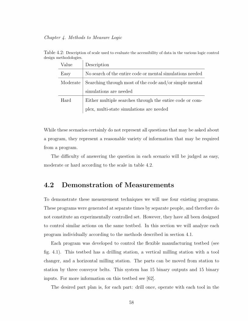
Chapter 4. Methods to Measure Logic
Table 4.2: Description of scale used to evaluate the accessibility of data in the various logic controldesign methodologies.
Value Description
Easy No search of the entire code or mental simulations needed
Moderate Searching through most of the code and/or simple mental
simulations are needed
Hard Either multiple searches through the entire code or com-
plex, multi-state simulations are needed
While these scenarios certainly do not represent all questions that may be asked about
a program, they represent a reasonable variety of information that may be required
from a program.
The difficulty of answering the question in each scenario will be judged as easy,
moderate or hard according to the scale in table 4.2.
4.2 Demonstration of Measurements
To demonstrate these measurement techniques we will use four existing programs.
These programs were generated at separate times by separate people, and therefore do
not constitute an experimentally controlled set. However, they have all been designed
to control similar actions on the same testbed. In this section we will analyze each
program individually according to the methods described in section 4.1.
Each program was developed to control the flexible manufacturing testbed (see
fig. 4.1). This testbed has a drilling station, a vertical milling station with a tool
changer, and a horizontal milling station. The parts can be moved from station to
station by three conveyor belts. This system has 15 binary outputs and 15 binary
inputs. For more information on this testbed see [62].
The desired part plan is, for each part: drill once, operate with each tool in the
58

Chapter 4. Methods to Measure Logic
Figure 4.1: Flexible manufacturing testbed. This machine consists of three stations with threeseparate conveyors used for part handling. The first station is a drilling station. The middlestation is a vertical milling station which includes a three position tool changer. The final stationis a horizontal milling station. This machine contains 15 inputs (4 infrared part sensors, 10 touchsensors, and 1 on/off switch) and 15 inputs (7 single direction motors and 4 bi-directional motors).
vertical tool changer, and then perform two passes with the horizontal mill. Parts
should be moved to the next station as soon as it is clear.
The programs were generated prior to this study and most have been previously
published.
4.2.1 Specification of Accessibility Scenarios
The accessibility of the program data will be determined by analyzing the difficulty
of answering the following questions about the controlled system. These scenarios are
specific examples of types of scenarios described in section 4.1.2.
Scenario 1 (Single Output Debugging)
Situation: The system is currently running, and the first conveyor has not turned on
when a new part was placed at the start.
Question: Why hasn’t the drill conveyor turned on?
This sort of question is often used as an example of why ladder diagrams are so
simple.
59
Chapter 4. Methods to Measure Logic
Scenario 2 (System Manipulation)
Situation: The system was processing a single part when that part was removed unex-
pectedly. The user must now manually depress sensors as needed to manipulate the
system state.
Question: What needs to be done to return the system to the “idle” state?
This should not be tried with a real system due to safety considerations, but it is
a reasonable approximation of situations which occur in industrial systems.
Scenario 3 (Desired System Behavior)
Situation: The user only has access to the logic and a description of the machine.
Question: What happens to a part after it has been drilled?
Scenario 4 (Unexpected System Behavior)
Situation: The user only has access to the logic and a description of the machine.
Question: What happens if an additional part is added to the vertical mill conveyor
mid-stream?
4.2.2 Analysis of a Ladder Diagram Solution
The ladder diagram was professionally generated by the manufacturer of the testbed [29].
The complete code can be found at [62].
4.2.2.1 Direct Measurements
The ladder diagram contains 27 separate rungs of code, and each rung represents a
distinct operation; therefore No = 27. The ladder diagram requires 4 latches (boolean
state variables), 2 counters and 2 timers. In addition, each of the 15 outputs can be
read by any rung, and effectively becomes a state variable. Therefore there are 23
state variables, therefore Ns = 23.
60
Chapter 4. Methods to Measure Logic
The rungs in the ladder diagram do not follow an obvious order, and there is
no separation of the ladder into separate parts. Therefore there is only one module,
containing 100% of the code, therefore Nm = 1 and S = 1.0.
In order to find all the causes or effects of a single rung, each rung of code must
be searched in turn. Therefore for this piece of code, 27 separate operations must be
searched to find all the causes or effects of a single operation. However, since each
output or state variable is controlled from a single rung, once a programmer is familiar
with the code he will be able to directly turn to a particular rung. Since there are an
average of 4.2 elements per rung, only 4.2 rungs on average need to be searched to
find all possible causes. Therefore ICc = 4.2 and ICe = 27. Note that many ladder
editors provide a “cross reference table” which maintains a list of all rungs which are
affected by an output or state variable, in addition to providing direct access to the
rung which maintains that output or state.
These numbers are summarized in table 4.3.
4.2.2.2 Accessibility of Data
Scenario 1, Single Output Debugging:
In this ladder diagram (as in most), each output is controlled by exactly one rung,
the position of which is usually known. Therefore, to determine why a particular
rung has not turned on, one needs to find the single appropriate rung, and examine
the inputs and state variables which affect it. In fact, some ladder programming
systems highlight the elements which are logically true, so that a quick visual scan
can determine the cause of the problem. In many cases the problem can be pinpointed
to a single input that is in the wrong state.
Since this problem requires neither searching the code or complex simulation, we
will judge it easy.
Scenario 2, System Manipulation:
While it is seems very easy to determine the cause of a single unexpected output, it
61

Chapter 4. Methods to Measure Logic
Drill Press
Lower Limit
Switch
Drill Done
Latch
Drill Done
Latch
Drill Press IR
Sensor
Drill Press
Timer
Vertical Mill
Upper Limit
Switch
Vertical Mill
Position Switch
Reset
Latch
Figure 4.2: Example of a single rung from the sample program: The Drill Done Latch will turnon when the drill press reaches its lower limit switch, and remains there for the duration of the drillpress timer. It will turn off when the Reset Latch is set, or the part leaves the drill press sensorand either reaches the vertical mill position switch, or the vertical mill leaves its upper limit switch.(All physical switches are normally closed.)
is not clear how the rungs relate to each other. This means that in general, it is very
difficult to plan more than one step into the future without substantial understanding
of the nature of the system.
However, this ladder diagram contains a very prominent latch called the Reset
Latch, which appears in 12 rungs. It is clear from a casual reading of the code that
the Reset Latch will cause the system to return to the “idle” state when the system
is powered down or the on/off switch is turned off.
Since this problem did not require and hard operations, it may be judged easy. It
should be noted that this problem was solved by the variable names chosen for the
program. A similar problem (e.g. cause the system to continue as if a removed part
never existed) would be require the operator to manually simulate the entire ladder
diagram, a hard operation.
Scenario 3, Desired System Behavior:
It is difficult to determine what will happen to the part after it has been drilled at
the first station. There is a latch called the Drill Done Latch which appears in the
rungs controlling the Vertical Mill Conveyor, the Drill Press Conveyor Motor,
and the drill press motors (both up and down). It seems reasonable to assume the
this latch is important to understanding this scenario, see figure 4.2.
62
Chapter 4. Methods to Measure Logic
This variable is set when the drill press has been on and the lower limit switch
for the duration specified in the Drill Press Timer (requires knowledge of the rung
controlling the Drill Press Timer, not shown). It is unset by the Reset Latch. It
can also be unset by both having no part at the Drill Press IR Sensor and either a
part at the Vertical Mill Position Switch or the vertical mill leaving it’s upper
position. That is, the drill is considered “done” from when the drill operation is
completed to when the part has left the drill station and arrived at the vertical mill
station. Therefore it stands to reason that that part moves to the vertical mill station
after it has been drilled.
This kind of reasoning must be continued through five additional rungs before
the actions on a part can be fully understood. The five rungs control: Vertical
Mill Head Motor Down, Vertical Drill Down Latch, Vertical Mill Conveyor
Motor, Vertical Mill Rotate Motor, and the Drill Count counter.
This scenario required the mental simulation of multiple independent rungs of the
logic. Therefore we will judge this problem hard.
Scenario 4, Unexpected System Behavior:
If an unexpected part is added where it can be detected by the Vertical Mill
Position Switch when the system is waiting for a part to arrive there, the effects
are easy to understand, since the system cannot distinguish the unexpected part
from the expected one. However, this will leave another part in the system. This
can be determined just from knowledge of the system, without consulting the ladder
diagram.
If the unexpected part arrives when no part is expected, it could potentially affect
all rungs which read that sensor. There are 4 such rungs. That sensor is used to:
1) Turn off the Drill Press Conveyor Motor when a part arrives
2) Turn off the Vertical Mill Conveyor Motor when a part arrives
3) Turn off the Vertical Drill Down Latch when a part leaves
4) Ensure that the vertical mill head only lowers when a part is present
63
Chapter 4. Methods to Measure Logic
In each of these cases, the arrival of an unexpected part does not immediately cause
a change of state. In addition, various interlocks (such as condition 4 above) ensure
that certain forbidden operations will never take place.
However, while it is not too difficult to determine that the arrival of an unexpected
part will not cause the system to crash, or forbidden operations to occur, it is not
clear from the code if the extra parts on the conveyor will ever clear themselves out,
or if there will always be an extra part between the drill and the vertical mill.
To solve this without running the program, the programmer would need to men-
tally simulate both the entire program and the testbed for many cycles. Therefore
we will judge this problem hard.
4.2.3 Analysis of a Petri Net Solution
The Petri net program for the testbed was generated by C. Gollapudi [18]. A portion
of the Petri net is shown in figure 4.3.
4.2.3.1 Direct Measurements
The Petri net contains 63 places and 49 transitions. Therefore the No = 49 and Ns =
63, since all states and operations are directly represented by places and transitions.
The program consists of three modules. It has a module for the drill station,
the vertical mill station, and the horizontal mill station. The largest module has 19
operations, or .38 of the total. Therefore Nm = 3 and S = 0.38.
The hidden dependency values are: ICc = 2.02 and ICe = 2.18. The program
consists primarily of transitions with one condition between two places with one
output. Therefore most of the transitions have two possible causes (the condition on
the transition and the previous transition) and two possible effects (the output on
the out-place and the next transition).
These values are summarized in table 4.3.
64
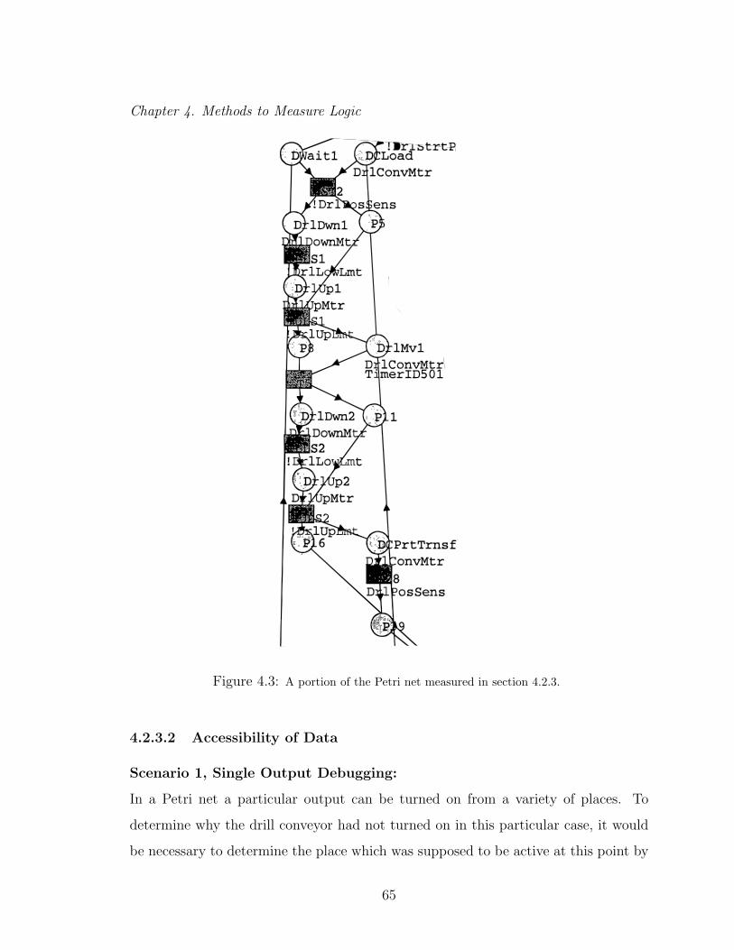
Chapter 4. Methods to Measure Logic
Figure 4.3: A portion of the Petri net measured in section 4.2.3.
4.2.3.2 Accessibility of Data
Scenario 1, Single Output Debugging:
In a Petri net a particular output can be turned on from a variety of places. To
determine why the drill conveyor had not turned on in this particular case, it would
be necessary to determine the place which was supposed to be active at this point by
65
Chapter 4. Methods to Measure Logic
searching the code. After finding the desired place, the programmer would need to
determine what condition was needed to activate that place from the current state.
Finding the desired place would require a search of all 16 places within the appropriate
module. Then the user would need to trace back to in the program path to the current
state, and determine the unsatisfied condition.
This requires a search of the entire code for the desired state, followed by rela-
tively simple reverse search for the missing condition. This problem will be judged
moderately difficult.
Scenario 2, System Manipulation:
In a Petri net the flow of the system can usually be determined easily from the
layout of the program. Therefore, given a current state, and a desired state, it is
generally straightforward to determine the quickest path to the desired state, and the
programmer then needs to check the condition of each transition in turn.
Therefore, since this requires neither searching nor mental simulation, this problem
is easy.
Scenario 3, Desired System Behavior:
Since Petri nets express a sequence of events, most sequential data is readily available.
For example the question “What does the drill do after it moves down?” is directly
available from the diagram. However sequential data based on the part is not as
readily available, since it relies on knowledge of the physical system. In this case,
after the part has been drilled each program waits for a synchronizing operation, and
then turns on the drill conveyor. The part then triggers a sensor in the next module
which starts the next operation.
In this scenario the user must perform a simple mental simulation of the part and
the program. However each is a simple sequential simulation and only need to cover
a couple of states. Therefore this problem is moderately difficult.
Scenario 4, Unexpected System Behavior:
As with the ladder diagram, from knowledge of the system sensors it can be deter-
66
Chapter 4. Methods to Measure Logic
mined that if the system is waiting for a part then the introduced part will be treated
as the expected one, leaving a part in the system. Because Petri nets only scan ex-
pected inputs, if the part is introduced at a sensor while no part is expected it will
be ignored by the system until some part is expected from the drill station. In this
case the drilled part will not be moved, and will effectively be another unexpected
part, now at the drill station.
However, to determine what will happen to the extra part from the Petri net
requires a mental simulation of the entire Petri net and the physical system over a
large number of interacting states. This problem is hard.
These measurements are summarized in table 4.4.
4.2.4 Analysis of Signal Interpreted Petri Nets (SIPNs)
The single signal interpreted Petri net sample was written by Stephane Klein [31], a
portion is shown in figure 2.5 on page 23.
4.2.4.1 Direct Measurements
The signal interpreted Petri net consists of 68 places and 50 transitions. Therefore
Ns = 68 and No = 50.
The program is built of one main Petri net with four subnets. Three of the subnets
have a single subnet of their own for a total of eight modules. The largest module,
which controls a single horizontal milling cycle, contains 10 operations. Therefore
Nm = 8 and S = 10/50 = 0.2.
The average number causes which must be searched to determine the cause of a
transition is 3.66. Most transitions must check one transition connected to its pre-
place, one transition connected to its post-place, and a condition on its input. Many
require more. The average number of effects which may be the result of a transition
is 7.34. This number is higher than the number for Petri nets because every output is
67
Chapter 4. Methods to Measure Logic
always explicitly defined in SIPN, whereas the program used in section 4.2.3 implied
that all outputs which were not turned on were turned off. If defining an output to
be off is not considered an effect, then the average number of effects to be searched is
3.30. Since this definition is closer to that used by other methodologies, we will use
ICc = 3.66 and ICe = 3.30.
4.2.4.2 Accessibility of Data
Scenario 1, Single Output Debugging:
There are two modules which control the drilling station of the testbed. These two
modules contain a total of 11 transitions and 15 places. Looking over the modules,
the first transition in the first module is the only one that turns on the drill con-
veyor. In addition this transition had no conditions. That makes this scenario seem
straightforward.
However, the drill module will not be made active unless all of the modules have
correctly completed their respective cycles. Therefore if the drill conveyor will not
start, most likely the problem is actually with one of the other modules. Therefore a
search of the other modules will be needed to determine where the program has hung
up.
Since this requires a search of most of the program, we will judge this scenario to
be moderately difficult.
Scenario 2, System Manipulation:
Manipulating the system of signal interpreted Petri nets is very similar to the more
typical Petri nets discussed in section 4.2.3.2. Therefore this problem will be judged
easy.
Scenario 3, Desired System Behavior:
The signal interpreted Petri net is laid out such that is very easy to determine what a
particular module will do next. However, as in the typical Petri net, to follow a part
through requires somewhat more work. In this case the user must have a minimal
68
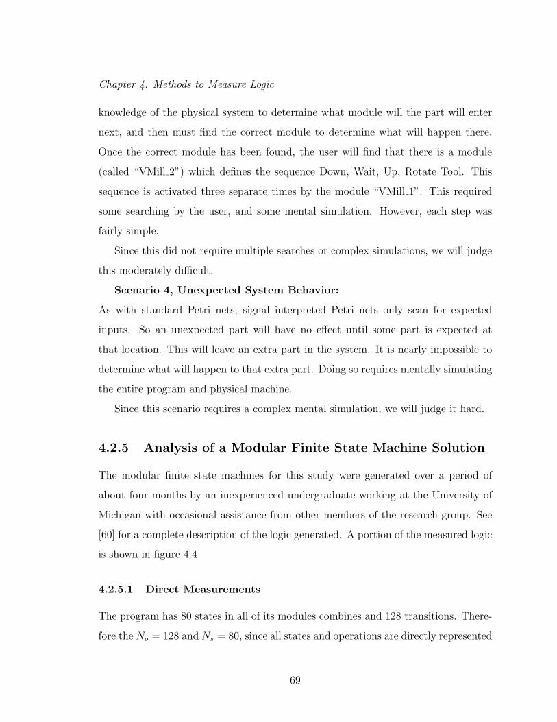
Chapter 4. Methods to Measure Logic
knowledge of the physical system to determine what module will the part will enter
next, and then must find the correct module to determine what will happen there.
Once the correct module has been found, the user will find that there is a module
(called “VMill 2”) which defines the sequence Down, Wait, Up, Rotate Tool. This
sequence is activated three separate times by the module “VMill 1”. This required
some searching by the user, and some mental simulation. However, each step was
fairly simple.
Since this did not require multiple searches or complex simulations, we will judge
this moderately difficult.
Scenario 4, Unexpected System Behavior:
As with standard Petri nets, signal interpreted Petri nets only scan for expected
inputs. So an unexpected part will have no effect until some part is expected at
that location. This will leave an extra part in the system. It is nearly impossible to
determine what will happen to that extra part. Doing so requires mentally simulating
the entire program and physical machine.
Since this scenario requires a complex mental simulation, we will judge it hard.
4.2.5 Analysis of a Modular Finite State Machine Solution
The modular finite state machines for this study were generated over a period of
about four months by an inexperienced undergraduate working at the University of
Michigan with occasional assistance from other members of the research group. See
[60] for a complete description of the logic generated. A portion of the measured logic
is shown in figure 4.4
4.2.5.1 Direct Measurements
The program has 80 states in all of its modules combines and 128 transitions. There-
fore the No = 128 and Ns = 80, since all states and operations are directly represented
69
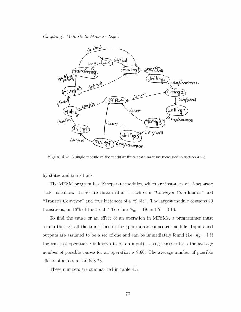
Chapter 4. Methods to Measure Logic
Figure 4.4: A single module of the modular finite state machine measured in section 4.2.5.
by states and transitions.
The MFSM program has 19 separate modules, which are instances of 13 separate
state machines. There are three instances each of a “Conveyor Coordinator” and
“Transfer Conveyor” and four instances of a “Slide”. The largest module contains 20
transitions, or 16% of the total. Therefore Nm = 19 and S = 0.16.
To find the cause or an effect of an operation in MFSMs, a programmer must
search through all the transitions in the appropriate connected module. Inputs and
outputs are assumed to be a set of one and can be immediately found (i.e. nic = 1 if
the cause of operation i is known to be an input). Using these criteria the average
number of possible causes for an operation is 9.60. The average number of possible
effects of an operation is 8.73.
These numbers are summarized in table 4.3.
70
Chapter 4. Methods to Measure Logic
4.2.5.2 Accessibility of Data
Scenario 1, Single Output Debugging:
In the MFSM framework, each output is controlled by a single module. To find the
reason that the conveyer has not turned on the programmer must look at the state
of the module controlling the drill conveyor, which is an instance of the “Transfer
Conveyor” module. Within this module there are 8 states and 20 transitions, and any
of the transitions can cause the conveyor to be turned on. Therefore the programmer
must determine which state the machine should be in, and which transitions need
to occur. Since the states are intelligently named the correct state can generally be
found. Then the programmer must determine what event must occur for the correct
transition to fire, and if needed follow that event back to the module generating it.
In total there are four modules between the start sensor and the command to turn
the conveyor on. These four modules contain a total of 31 states and 56 transitions.
While each module has a limited number of states to search though, and intelligent
names should help considerably, there are still four possible modules which could be
the cause of the problem. This is a considerable search, and therefore this problem
is hard.
Scenario 2, System Manipulation:
To manipulate this system back to the idle state all 19 interconnected modules must be
manipulated, even those which do not have direct I/O points, but are only controlled
through other modules. This will involve the mental simulation of the entire system
of 19 modules. This process can be simplified somewhat by manipulating only a few
of the modules and trusting the program to manipulate the rest, however this is still
not an easy task.
An easier method, if the exact error is known, is to simulate the motion of the
removed block through the conveyors. This method utilizes a mental model of the
controlled physical system, not the program. It will also not work if the exact error
is not known.
71
Chapter 4. Methods to Measure Logic
While generating this program the most common observed method of dealing with
this problem was to trip the infrared part sensors haphazardly until either the part
system was in the correct state or the user gave up and restarted the program.
Since this involves a complex simulation, this problem is hard.
Scenario 3, Desired System Behavior:
To determine what happens to a part after it has been drilled, a programmer would
first need to examine the drill control plan module. That module demonstrates ex-
plicitly that the part will be drilled another three times after its first drill. That
information is very accessible.
This does not involve any searches or mental simulation, so this problem is easy.
Scenario 4, Unexpected System Behavior:
To determine what will happen if a part is added unexpectedly might involve a full
mental simulation of the entire controller/system combination. Most of the informa-
tion needed can be obtained from the conveyor coordinators, which are three instances
of a single conveyor coordinator module. (This module has 6 states and 9 transitions.)
However, even with this simplification this requires a mental simulation of three fairly
complex modules.
This problem is hard.
4.2.6 Summary of Measurements
Measurements of the sample programs are shown in tables 4.3 and 4.2.
The size of the program (measured either by number of states or number of op-
erations) appears inversely related to its modularity. Petri nets are the most simply
connected, followed by signal interpreted Petri nets, modular finite state machines,
and ladder diagrams. Each framework seems to be good at at some scenarios, while
poor at others. This agrees with the “match-mismatch hypothesis” [17] which noted
that “subjects performed best on ‘matched pairs’ of tasks and languages”.
These measures were, and always must be, based on existing samples of logic. It is
72
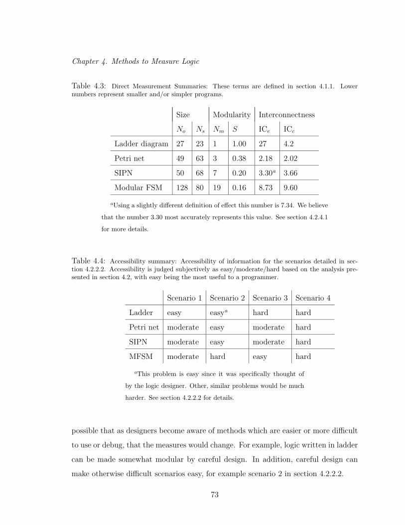
Chapter 4. Methods to Measure Logic
Table 4.3: Direct Measurement Summaries: These terms are defined in section 4.1.1. Lowernumbers represent smaller and/or simpler programs.
Size Modularity Interconnectness
No Ns Nm S ICe ICc
Ladder diagram 27 23 1 1.00 27 4.2
Petri net 49 63 3 0.38 2.18 2.02
SIPN 50 68 7 0.20 3.30a 3.66
Modular FSM 128 80 19 0.16 8.73 9.60
aUsing a slightly different definition of effect this number is 7.34. We believe
that the number 3.30 most accurately represents this value. See section 4.2.4.1
for more details.
Table 4.4: Accessibility summary: Accessibility of information for the scenarios detailed in sec-tion 4.2.2.2. Accessibility is judged subjectively as easy/moderate/hard based on the analysis pre-sented in section 4.2, with easy being the most useful to a programmer.
Scenario 1 Scenario 2 Scenario 3 Scenario 4
Ladder easy easya hard hard
Petri net moderate easy moderate hard
SIPN moderate easy moderate hard
MFSM moderate hard easy hard
aThis problem is easy since it was specifically thought of
by the logic designer. Other, similar problems would be much
harder. See section 4.2.2.2 for details.
possible that as designers become aware of methods which are easier or more difficult
to use or debug, that the measures would change. For example, logic written in ladder
can be made somewhat modular by careful design. In addition, careful design can
make otherwise difficult scenarios easy, for example scenario 2 in section 4.2.2.2.
73
Chapter 4. Methods to Measure Logic
4.3 Comparing these measurements to previous aca-
demic measurements
The measurements described and demonstrated in this chapter generally show that
the size of a ladder diagram is less than an equivalent Petri net. This is in contrast to
two previously published measurement methods. The “basic element approach” [65]
and the “if-then transform” [34] both show that the size of a ladder diagram is greater
than that of an equivalent Petri net.
There are a few possible causes of this inconsistency. The first is that the examples
used by the different researchers are somehow different. For example, a ladder diagram
generated by a Petri net expert may be fundamentally different than one generated
by a ladder expert, although no evidence of such bias can be found in the examples.
A second possibility is that the measurements are somehow different, and tend to
favor one methodology vs. another. A final possibility is that this inconsistency is
due to the small sample size of the measured logic, and would resolve itself with more
measurements.
To address this question, the examples from this work, as well as those used in [65]
and [34], have been measured using the two measurements of size presented in this
work (see page 54) as well as the measurements presented in [65] and [34]. There are
a total of six measurements of size, two from each source. These are:
From this work
Operations The number of inseparable actions possible
State Variables The number of state variables required
From the “Basic element approach” [65]
Nodes The number of graphical nodes needed
Links The number of connections between the nodes
74

Chapter 4. Methods to Measure Logic
From the “if-then transform” [34]
Rules The number of boolean rules required to represent the logic
Operators The number of operators (including parentheses) required to rep-
resent the logic
The resulting measurements are shown in table 4.5
There are a few things to note about the measurements. The number of boolean
rules required is always the same as the number of operations. This is not surprising
since each operation is generally converted into one boolean rule. In addition, the
number of operators is very similar to the number of nodes, which is not obvious from
the definitions. This is caused by the straightforward method of creating boolean ex-
pressions, where each node usually represents one additional condition (including one
operator) in a boolean rule. But most interesting to this discussion, the measurement
of operations, state variables, and rules tend to show that Petri nets are a larger
representation than ladder diagrams, and the measurement of nodes, links, and oper-
ators tend to show that Petri nets are a smaller representation than ladder diagrams.
This is shown explicitly in table 4.6.
Thus, these measurements are not consistent in whether Petri nets or ladder dia-
grams are a more compact representation of logic control code. In addition the mea-
surements of modularity, interconnectedness, and accessibility of data have shown
that there are advantages and disadvantages to different logic control design method-
ologies depending on the circumstances and the measurement chosen. To provide
context to the measurements, it is necessary to examine how the methodologies will
be used, thus determining what measurements will allow for faster, more reliable logic
generation.
The true judge of a measurement is how useful it is to the person using it. Op-
erators, states, and nodes all represent things which must be explicitly created by a
logic designer. Links in a ladder diagram do not need to be explicitly created by the
75
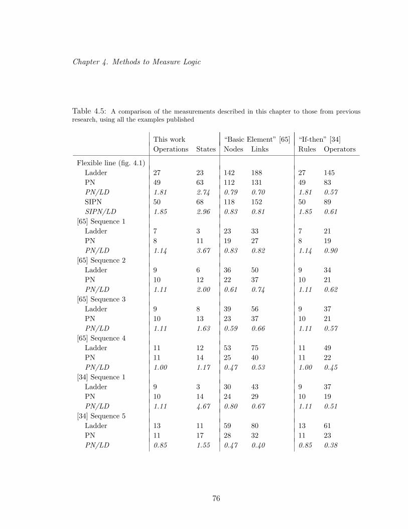
Chapter 4. Methods to Measure Logic
Table 4.5: A comparison of the measurements described in this chapter to those from previousresearch, using all the examples published
This work “Basic Element” [65] “If-then” [34]Operations States Nodes Links Rules Operators
Flexible line (fig. 4.1)Ladder 27 23 142 188 27 145PN 49 63 112 131 49 83PN/LD 1.81 2.74 0.79 0.70 1.81 0.57SIPN 50 68 118 152 50 89SIPN/LD 1.85 2.96 0.83 0.81 1.85 0.61
[65] Sequence 1Ladder 7 3 23 33 7 21PN 8 11 19 27 8 19PN/LD 1.14 3.67 0.83 0.82 1.14 0.90
[65] Sequence 2Ladder 9 6 36 50 9 34PN 10 12 22 37 10 21PN/LD 1.11 2.00 0.61 0.74 1.11 0.62
[65] Sequence 3Ladder 9 8 39 56 9 37PN 10 13 23 37 10 21PN/LD 1.11 1.63 0.59 0.66 1.11 0.57
[65] Sequence 4Ladder 11 12 53 75 11 49PN 11 14 25 40 11 22PN/LD 1.00 1.17 0.47 0.53 1.00 0.45
[34] Sequence 1Ladder 9 3 30 43 9 37PN 10 14 24 29 10 19PN/LD 1.11 4.67 0.80 0.67 1.11 0.51
[34] Sequence 5Ladder 13 11 59 80 13 61PN 11 17 28 32 11 23PN/LD 0.85 1.55 0.47 0.40 0.85 0.38
76
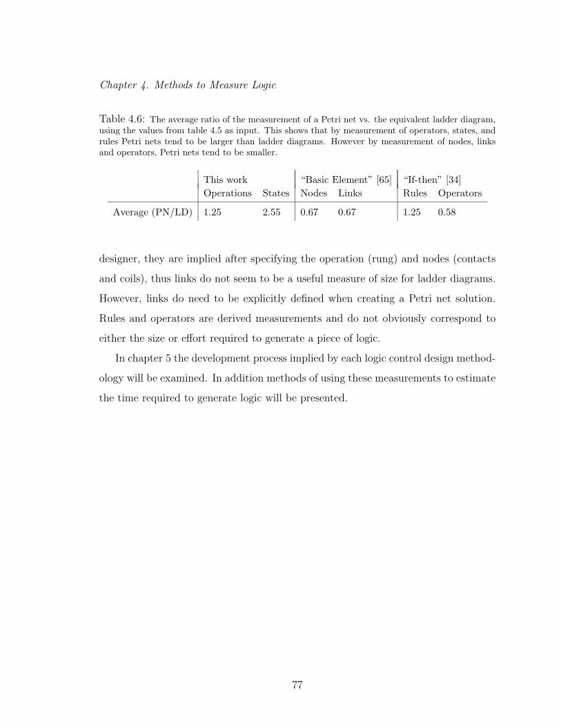
Chapter 4. Methods to Measure Logic
Table 4.6: The average ratio of the measurement of a Petri net vs. the equivalent ladder diagram,using the values from table 4.5 as input. This shows that by measurement of operators, states, andrules Petri nets tend to be larger than ladder diagrams. However by measurement of nodes, linksand operators, Petri nets tend to be smaller.
This work “Basic Element” [65] “If-then” [34]Operations States Nodes Links Rules Operators
Average (PN/LD) 1.25 2.55 0.67 0.67 1.25 0.58
designer, they are implied after specifying the operation (rung) and nodes (contacts
and coils), thus links do not seem to be a useful measure of size for ladder diagrams.
However, links do need to be explicitly defined when creating a Petri net solution.
Rules and operators are derived measurements and do not obviously correspond to
either the size or effort required to generate a piece of logic.
In chapter 5 the development process implied by each logic control design method-
ology will be examined. In addition methods of using these measurements to estimate
the time required to generate logic will be presented.
77
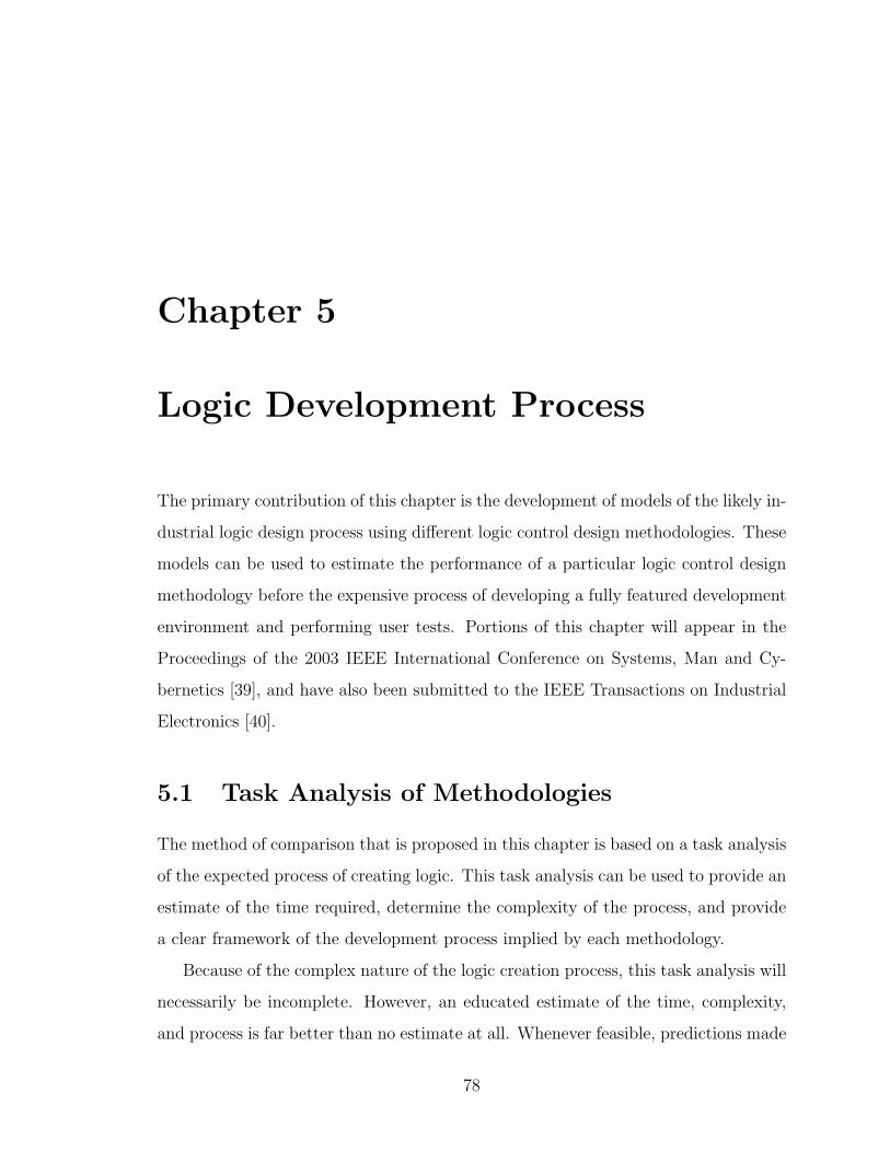
Chapter 5
Logic Development Process
The primary contribution of this chapter is the development of models of the likely in-
dustrial logic design process using different logic control design methodologies. These
models can be used to estimate the performance of a particular logic control design
methodology before the expensive process of developing a fully featured development
environment and performing user tests. Portions of this chapter will appear in the
Proceedings of the 2003 IEEE International Conference on Systems, Man and Cy-
bernetics [39], and have also been submitted to the IEEE Transactions on Industrial
Electronics [40].
5.1 Task Analysis of Methodologies
The method of comparison that is proposed in this chapter is based on a task analysis
of the expected process of creating logic. This task analysis can be used to provide an
estimate of the time required, determine the complexity of the process, and provide
a clear framework of the development process implied by each methodology.
Because of the complex nature of the logic creation process, this task analysis will
necessarily be incomplete. However, an educated estimate of the time, complexity,
and process is far better than no estimate at all. Whenever feasible, predictions made
78

Chapter 5. Logic Development Process
by task analysis methods should be validated either by informal trials or by structured
experiments.
This chapter will describe the sequence of tasks required for logic development for
each logic control design methodology of interest. This description will focus on the
sequence likely to be used in an industrial development setting, where machines are of-
ten similar to previous projects and reliability is more important than features. Using
this sequence together with empirical measurements of previous developments, this
work can estimate the time required to create logic and also compare the complexity
of the process and likely debugging scenarios.
The most basic measurement is the estimate of time required to complete a logic
design problem using each logic control design methodology. Equation 5.1 is used to
estimate total time T required of the lead developer.
T =1
λ
∑
∀α∈A
nατα (5.1)
λ = fraction of lead developer’s time spent in development
A = set of development activities required
τα = average time to complete one instance of α
nα = number of times α must be performed
The coefficient λ represents the amount of time that the lead developer actually
spends creating logic. Other activities that he may be required to perform are memory
management, communicating with other team members, and retrieving specification
documents (covered in section 3.2.2 on page 31). These activities are unstructured
by nature, and no additional framework will be provided for them. The coefficient λ
has been observed empirically for one instance of ladder diagrams in chapter 3, and
estimates for Petri nets and modular finite state machines will be based on that.
The set A includes all activities directly related to creating logic, primarily entering
the elements needed to represent the logic.
79

Chapter 5. Logic Development Process
5.1.1 Ladder Diagrams
5.1.1.1 Creation
Since ladder diagrams are the industry standard, a fairly detailed description of the
logic generation process can be made. Previous work on the task analysis of ladder
development (chapter 3) indicates that the process of generating ladder diagrams can
be represented by the flow chart in figure 5.1 (also shown in figure 3.8 on page 44).
According to this study the lead developer, who is responsible for creating system level
logic as well as a representative sample of the logic needed for each station, spends
about 28% of his development time actually generating logic, with the balance of time
spent in project coordination (44%), memory management (15%) and other activities
(13%), including file maintenance and minimal debugging. Therefore λLD = 0.28.
There are three separate methods by which rungs are developed: new development
(nd), electronic copy (ec), and manual copy (mc). Therefore the set of activities
required to generate ladder logic is ALD = {nd, ec, mc}. The estimated time to
complete a logic design problem using ladder diagrams is:
TLD = 1λLD
(nndτnd + necτec + nmcτmc) (5.2)
with parameter estimates of:
λLD = 0.28
τnd = 20 min
τec = 2.5 min
τmc = 4 min
nnd = 0.05 × ntot
nec = 0.24 × ntot
nmc = 0.71 × ntot
(5.3)
where:
ntot = total number of rungs
80
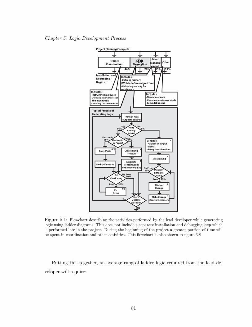
Chapter 5. Logic Development Process
44%
ProjectCoordination
Mem.Manage-Manage-
ment15%
Other
13%28%
Installation andDebugging Begins
Project Planning Complete
Copy/Paste
Think of nextoutput to control
RungAlready Exists?
Electronic or Paper?
Create Rung structure
Modify if neededAssociate
contacts/coilswith memory map
Consider:-Purpose of output-Inputs-Safety considerations
Create Rung
Think ofChange
Check rung
Mentally Simulate
Rung
FixErrors
Make Change(structure, memory)
MoreOutputsNeeded?
NoYes
PaperElectronic
No Error
Error
No Error
Error
No
Yes
25% 75%
25%
75%
50%
4
2
1
1
0.5
4
0.5
1
1
2
0.5
50%
5%95%
Typical Process of Generating Logic
Includes:-Instructing Employees-Defining inter-processor communication-Creating Documentation
Includes:-Defining memory
(Which defines algorithm)-Validating memory forconsistancy
Includes:-File maintenance-Updating previous projects-Some debugging
Figure 5.1: Flowchart describing the activities performed by the lead developer while generatinglogic using ladder diagrams. This does not include a separate installation and debugging step whichis performed late in the project. During the beginning of the project a greater portion of time willbe spent in coordination and other activities. This flowchart is also shown in figure 3.8
Putting this together, an average rung of ladder logic required from the lead de-
veloper will require:
81
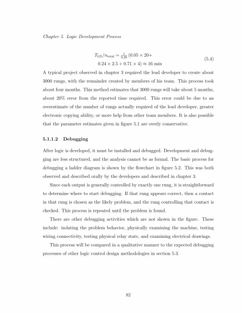
Chapter 5. Logic Development Process
TLD/ntotal = 10.28
(0.05 × 20+
0.24 × 2.5 + 0.71 × 4) ≈ 16 min(5.4)
A typical project observed in chapter 3 required the lead developer to create about
3000 rungs, with the remainder created by members of his team. This process took
about four months. This method estimates that 3000 rungs will take about 5 months,
about 20% error from the reported time required. This error could be due to an
overestimate of the number of rungs actually required of the lead developer, greater
electronic copying ability, or more help from other team members. It is also possible
that the parameter estimates given in figure 5.1 are overly conservative.
5.1.1.2 Debugging
After logic is developed, it must be installed and debugged. Development and debug-
ging are less structured, and the analysis cannot be as formal. The basic process for
debugging a ladder diagram is shown by the flowchart in figure 5.2. This was both
observed and described orally by the developers and described in chapter 3.
Since each output is generally controlled by exactly one rung, it is straightforward
to determine where to start debugging. If that rung appears correct, then a contact
in that rung is chosen as the likely problem, and the rung controlling that contact is
checked. This process is repeated until the problem is found.
There are other debugging activities which are not shown in the figure. These
include: isolating the problem behavior, physically examining the machine, testing
wiring connectivity, testing physical relay state, and examining electrical drawings.
This process will be compared in a qualitative manner to the expected debugging
processes of other logic control design methodologies in section 5.3.
82
Chapter 5. Logic Development Process
Think of nextbehavior to check
BehaviorCorrect?Yes
Check behavior
Find incorrectoutput rung
Find incorrectcontact on rung
Error inthis rung?
Find rung whichcontrols contact
Fix Error
No
Yes
No
Figure 5.2: Flowchart describing the activities performed to debug systems developed using ladderdiagrams. This process was both described by engineers responsible for debugging a project, anddirectly observed.
5.1.1.3 Validating Time Estimates Using a Keystroke Level GOMS Model
If needed, the time estimates for each step can be validated by using a more detailed
representation. As an example of this we consider the step “Create Rung Structure”
from figure 5.1. This is the process of creating the basic elements of the rung (bare
rung, contacts, branches, and coil) while looking at a printed template; this process
was estimated to take one minute of designer time.
To validate this estimate, we will provide a detailed representation of what this
process involves. We must assume that we know the details of a graphical user
interface (we have chosen a fairly representative sample), then we can estimate the
time required to achieve the goal using previously derived times. Card, Morann and
Newell [4] found and validated the time estimates shown in table 5.1.
A detailed representation of the process used to create the skeleton for a single
rung of this may be:
83

Chapter 5. Logic Development Process
Table 5.1: Time estimates of low level user operations as described in [4]
Operation Time
K Single keystroke by average user (not a typist). .28 sec.
B Single mouse click .20 sec.
M Single mental operator (e.g. retrieve data from long term memory) 1.35 sec.
P Pointing the mouse at something small 1.1 sec. a
H Moving hands from the keyboard to the mouse 0.40 sec.
A Acquire next task from a manuscript 4 sec.
Am Acquire next task from memory 0.5 sec.
aThis is actually more accurately described using Fitt’s law [3, 13], where the time, T , to
point at an object of size s and at a distance d while using a mouse is described as T =
0.8 + 0.1 log2
(ds + 0.5
)sec. In the interest of simplicity, we will use the 1.1 sec. approximation.
1. Create bare rung (usually created in groups of about 10)
(a) Click on “new rung” tool (M+P+B)/10
(b) Click 10 times in the main programming area (M/10)+B
2. Add coil to current rung (also created in groups of about 10)
(a) Click on “coil” tool (M+P+B)/10
(b) Click on rung (M/10)+(P+B)
3. Create needed branch structure of current rung (generally about 2 branches areneeded, which can all be held in working memory at once [5].)
(a) Click on “New Branch” tool (M+P+B)
(b) Look at branches required (if no branch required, goto 4) A
(c) Remember next branch Am
(d) Drag out branch M
i. Move mouse to left point of branch location Pii. Click and hold Biii. Move branch to right point of branch location Piv. Release B
(e) Goto 3c (Once per branch)
84
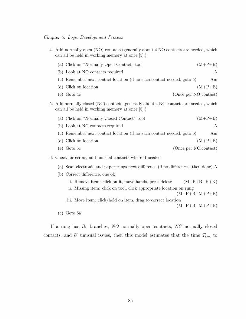
Chapter 5. Logic Development Process
4. Add normally open (NO) contacts (generally about 4 NO contacts are needed, whichcan all be held in working memory at once [5].)
(a) Click on “Normally Open Contact” tool (M+P+B)
(b) Look at NO contacts required A
(c) Remember next contact location (if no such contact needed, goto 5) Am
(d) Click on location (M+P+B)
(e) Goto 4c (Once per NO contact)
5. Add normally closed (NC) contacts (generally about 4 NC contacts are needed, whichcan all be held in working memory at once [5].)
(a) Click on “Normally Closed Contact” tool (M+P+B)
(b) Look at NC contacts required A
(c) Remember next contact location (if no such contact needed, goto 6) Am
(d) Click on location (M+P+B)
(e) Goto 5c (Once per NC contact)
6. Check for errors, add unusual contacts where if needed
(a) Scan electronic and paper rungs next difference (if no differences, then done) A
(b) Correct difference, one of:
i. Remove item: click on it, move hands, press delete (M+P+B+H+K)ii. Missing item: click on tool, click appropriate location on rung
(M+P+B+M+P+B)iii. Move item: click/hold on item, drag to correct location
(M+P+B+M+P+B)
(c) Goto 6a
If a rung has Br branches, NO normally open contacts, NC normally closed
contacts, and U unusual issues, then this model estimates that the time Tskel to
85
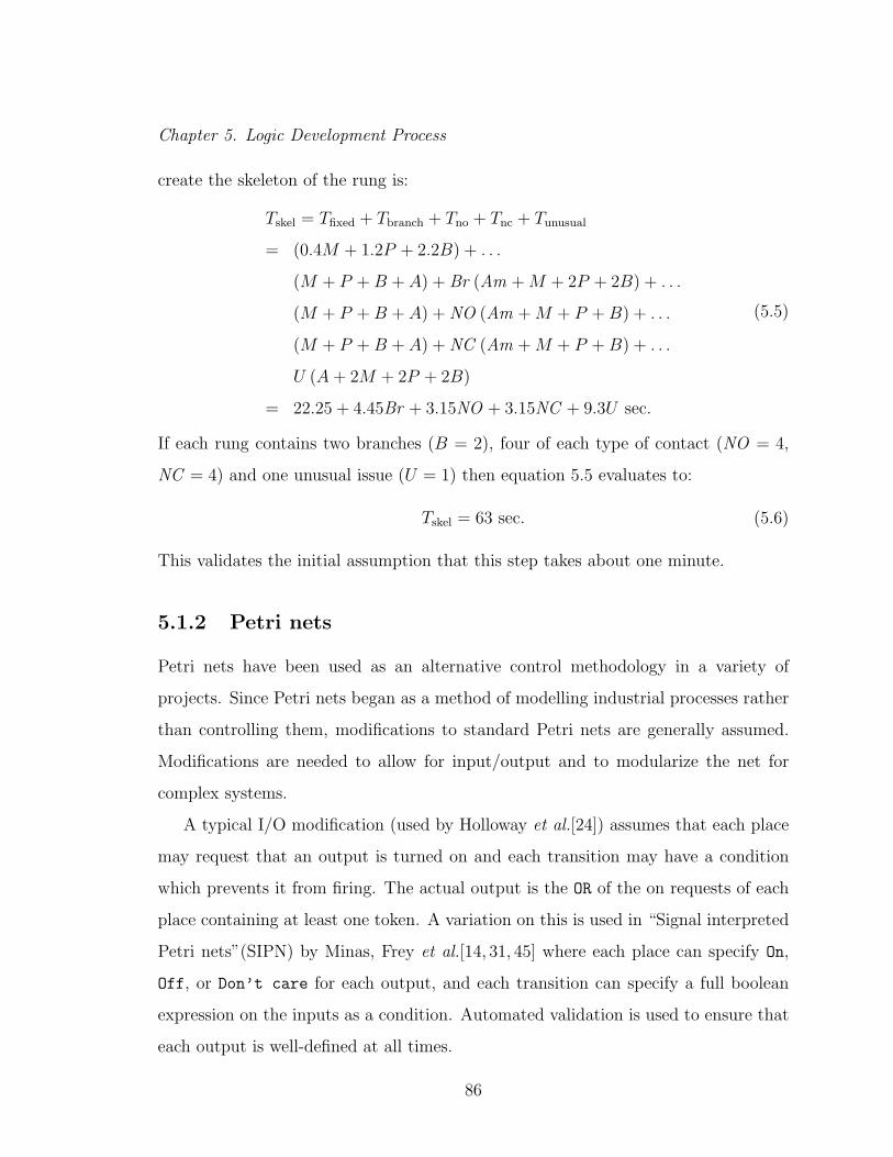
Chapter 5. Logic Development Process
create the skeleton of the rung is:
Tskel = Tfixed + Tbranch + Tno + Tnc + Tunusual
= (0.4M + 1.2P + 2.2B) + . . .
(M + P + B + A) + Br (Am + M + 2P + 2B) + . . .
(M + P + B + A) + NO (Am + M + P + B) + . . .
(M + P + B + A) + NC (Am + M + P + B) + . . .
U (A + 2M + 2P + 2B)
= 22.25 + 4.45Br + 3.15NO + 3.15NC + 9.3U sec.
(5.5)
If each rung contains two branches (B = 2), four of each type of contact (NO = 4,
NC = 4) and one unusual issue (U = 1) then equation 5.5 evaluates to:
Tskel = 63 sec. (5.6)
This validates the initial assumption that this step takes about one minute.
5.1.2 Petri nets
Petri nets have been used as an alternative control methodology in a variety of
projects. Since Petri nets began as a method of modelling industrial processes rather
than controlling them, modifications to standard Petri nets are generally assumed.
Modifications are needed to allow for input/output and to modularize the net for
complex systems.
A typical I/O modification (used by Holloway et al.[24]) assumes that each place
may request that an output is turned on and each transition may have a condition
which prevents it from firing. The actual output is the OR of the on requests of each
place containing at least one token. A variation on this is used in “Signal interpreted
Petri nets”(SIPN) by Minas, Frey et al.[14, 31, 45] where each place can specify On,
Off, or Don’t care for each output, and each transition can specify a full boolean
expression on the inputs as a condition. Automated validation is used to ensure that
each output is well-defined at all times.
86

Chapter 5. Logic Development Process
There are two main forms of modularization assumptions. The first, used in SIPN,
allows for a series of places to be combined into a single meta place. This works well
to encapsulate a simple sequence in a Petri net, although special care must be taken
to allow for early termination of that sequence (e.g. emergency stops). A second
method, used by Holoway et al., of modularizing Petri nets is to allow multiple Petri
nets to be run simultaneously, and the outputs of one Petri net can be considered the
inputs of another. This is better suited to systems where multiple processors may be
needed, although it is unclear if standard Petri net verification schemes still apply,
due to possible asynchronous behavior.
Both examples of Petri nets are likely to yield a similar development process,
shown here.
5.1.2.1 Creation
The basic method of creating Petri nets is shown in figure 5.3. This does not include
time spent in high level planning, setting up the I/O, project coordination or any
other activities. On this flow chart the approximate time (in minutes) to complete
each task is shown. In addition an estimate is made at each decision point of the
chance of taking each branch.
The development flowchart of Petri nets can be divided into the following sub-
activities: creating structures, new (ns), manual copy (mc), electronic copy (ec);
creating places (p); and creating transitions (t). Places and transitions do not need
to be created for electronically copied (ec) structures.
We have chosen not to add the time to create places and transitions to the time
needed to create structures. While creating structures is an important and time
consuming activity, the nature of structures in Petri nets can be very ambiguous. By
counting the number of places and transitions directly we can minimize the effects of
improperly counted structures.
The time required for memory management has been reduced by half from the
87
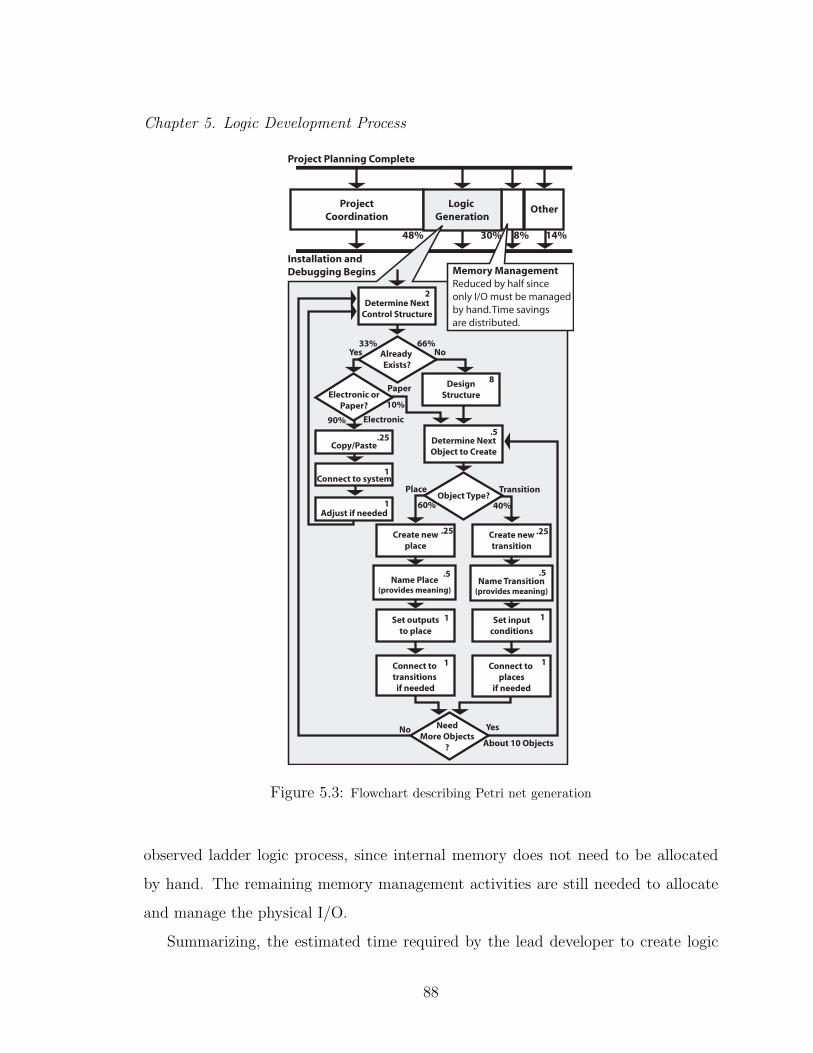
Chapter 5. Logic Development Process
48%
ProjectCoordination
8%
Other
14%30%
Logic Generation
Installation andDebugging Begins
Project Planning Complete
NeedMore Objects
?
Connect to transitions
if needed
Set outputsto place
Name Place(provides meaning)
Name Transition(provides meaning)
Create newplace
Object Type?
Determine NextObject to Create
Connect to places
if needed
Set inputconditions
Create newtransition
No Yes
Place Transition
Already Exists?
Determine NextControl Structure
Electronic orPaper?
Copy/Paste
Connect to system
DesignStructure
8
1
2
.25
.25
.5
.5
1
.25
1 1
.5
1
10%
33% 66%
90%
60% 40%
Electronic
Paper
About 10 Objects
NoYes
Adjust if needed1
Memory ManagementReduced by half since only I/O must be managed by hand. Time savings are distributed.
Figure 5.3: Flowchart describing Petri net generation
observed ladder logic process, since internal memory does not need to be allocated
by hand. The remaining memory management activities are still needed to allocate
and manage the physical I/O.
Summarizing, the estimated time required by the lead developer to create logic
88

Chapter 5. Logic Development Process
using Petri nets is:
Tpn = 1λpn
(nnsτns + nmcτmc + . . .
necτec + npτp + ntτt)(5.7)
with parameter estimates of:
λPN = 0.30
τns = 10.51 min
τmc = 2.51 min
τec = 4.25 min
τp = 3.25 min
τt = 3.25 min
(5.8)
Therefore the estimated time required to create a Petri net controller is:
1
0.30(10.5nns + 2.5nmc + 4.25nec + 3.25np + 3.25nt)
5.1.2.2 Debugging
Figure 5.4 shows a similar analysis for the probable method which would be used to
debug a system designed using Petri nets. Compare this to the method which has
been observed in ladders (see fig. 5.2). Much of the structure is the same, however
the activity find incorrect output rung has been replaced with Search for the
source of error. Since outputs in ladder are always driven by exactly one rung
and outputs in Petri nets can be driven by any number of places, this may be a more
difficult operation.
Most of the unstructured activities which were described for ladder diagrams will
also be present while debugging Petri nets. Likely errors include: unhandled and/or
forgotten events; improper place/transition labelling; and incorrect or poorly struc-
tured Petri nets. Some of these problems may be found with automated validation,
1These are the estimates of the time needed for each structure, not including the time required
to manually enter the places and transitions which the structure contains.
89
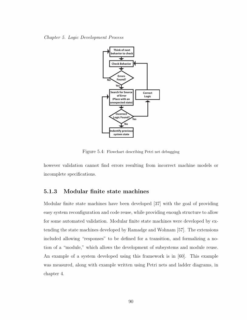
Chapter 5. Logic Development Process
Indentify previoussystem state
Search for Source of Error
(Place with an unexpected state)
Check Behavior
ErrorsFound?
IncorrectLogic Found?
CorrectLogic
No
Yes
No
Yes
Think of nextbehavior to check
Figure 5.4: Flowchart describing Petri net debugging
however validation cannot find errors resulting from incorrect machine models or
incomplete specifications.
5.1.3 Modular finite state machines
Modular finite state machines have been developed [37] with the goal of providing
easy system reconfiguration and code reuse, while providing enough structure to allow
for some automated validation. Modular finite state machines were developed by ex-
tending the state machines developed by Ramadge and Wohnam [57]. The extensions
included allowing “responses” to be defined for a transition, and formalizing a no-
tion of a “module,” which allows the development of subsystems and module reuse.
An example of a system developed using this framework is in [60]. This example
was measured, along with example written using Petri nets and ladder diagrams, in
chapter 4.
90
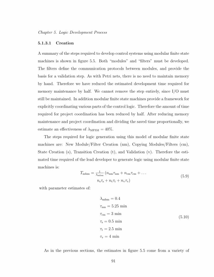
Chapter 5. Logic Development Process
5.1.3.1 Creation
A summary of the steps required to develop control systems using modular finite state
machines is shown in figure 5.5. Both “modules” and “filters” must be developed.
The filters define the communication protocols between modules, and provide the
basis for a validation step. As with Petri nets, there is no need to maintain memory
by hand. Therefore we have reduced the estimated development time required for
memory maintenance by half. We cannot remove the step entirely, since I/O must
still be maintained. In addition modular finite state machines provide a framework for
explicitly coordinating various parts of the control logic. Therefore the amount of time
required for project coordination has been reduced by half. After reducing memory
maintenance and project coordination and dividing the saved time proportionally, we
estimate an effectiveness of λMFSM = 40%.
The steps required for logic generation using this model of modular finite state
machines are: New Module/Filter Creation (nm), Copying Modules/Filters (cm),
State Creation (s), Transition Creation (t), and Validation (v). Therefore the esti-
mated time required of the lead developer to generate logic using modular finite state
machines is:
Tmfsm = 1λmfsm
(nnmτnm + ncmτcm + . . .
nsτs + ntτt + nvτv)(5.9)
with parameter estimates of:
λmfsm = 0.4
τnm = 5.25 min
τcm = 3 min
τs = 0.5 min
τt = 2.5 min
τv = 4 min
(5.10)
As in the previous sections, the estimates in figure 5.5 come from a variety of
91
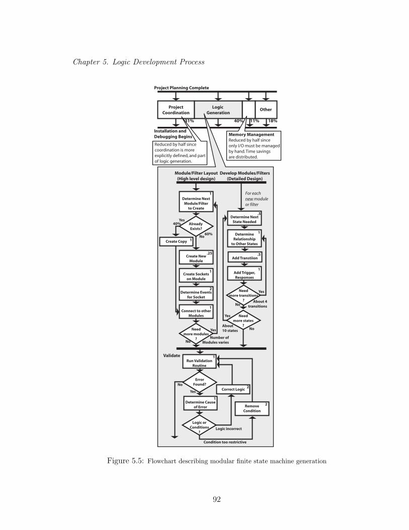
Chapter 5. Logic Development Process
31% 18%40%
ProjectCoordination
11%
OtherLogic Generation
Installation andDebugging Begins
Project Planning Complete
Determine NextState Needed
No
Yes
Develop Modules/Filters(Detailed Design)
Add Trigger,Responses
Add Transtiion
DetermineRelationship
to Other States
Needmore transitions
?
No
For eachnew moduleor filter
Needmore states
?
Validate
Determine Causeof Error
Run ValidationRoutine
Logic orConditions
?
Correct Logic
RemoveCondition
ErrorFound?No
Yes
Needmore modules
?
Connect to otherModules
Module/Filter Layout(High level design)
Determine Eventsfor Socket
Create Socketson Module
Create Copy
Create NewModule
Already Exists?
Determine NextModule/Filter
to Create
NoNumber of
Modules varies
No
Yes
.25
1
2
1
1
.5
.5
1
1
1
1
2
2
1
Condition too restrictive
Yes
Logic incorrect
60%
Yes
40%
About10 states
About 4transitions
Memory ManagementReduced by half since only I/O must be managed by hand. Time savings are distributed.
Reduced by half since coordination is more explicitly defined, and partof logic generation.
Figure 5.5: Flowchart describing modular finite state machine generation
92

Chapter 5. Logic Development Process
Indentify nextmodule to check
Identify ModuleControlling
Error Output
Check Behavior
ErrorsFound?
ErrorFound?
CorrectError
No
Yes
No
Yes
Think of nextbehavior to check
Search for error:Misdirected transition?Improper transition labeling?Structural problem?
Figure 5.6: Flowchart describing modular finite state machine debugging
sources. The number of modules which can be copied or reused comes from the
project developed for [60] and measured in chapter 4. Average numbers of states
in each module, and transitions from each state are derived from the same project.
The time required to create each item is an estimate based on our experience devel-
oping controllers in this framework. Existing validation tools (described in [9]) do
not provide a development environment, so all existing development has been done
using paper and pencil. The lack of full-featured development software means that
estimated times cannot yet be validated experimentally.
5.1.3.2 Debugging
The process for debugging modular finite state machines is slightly more complicated
than the process of debugging either Petri nets or ladder diagrams. The module
containing the error must be identified, and the error within that module found.
93

Chapter 5. Logic Development Process
Experience observing students developing modular finite state machines indicates
that often the cause of an error must often be tracked through three to four modules.
However, even limited validation tools usually find most errors, except those which
are due to conceptual errors in the logic structure. In addition, reuse of modules
should reduce the number of errors, although the number of development projects to
date has been too small to validate this hypothesis.
5.2 Program Size
The estimates of the time required to generate a program in section 5.1 depend on
the size of the program required. Current methods to estimate this size a priori
are limited. For this work empirically derived results are used. Future methods of
extrapolating these results to other programs are discussed here, however a rigorous
treatment is left to future work.
5.2.1 Empirical Measurements of Existing Programs
This work uses empirical measurements of existing programs written to control the
same system using the three logic control design methodologies described, (see chap-
ter 4). The programs were written to control a testbed containing 15 binary inputs
and 15 binary outputs. The ladder diagram was written professionally by the man-
ufacturer, the Petri net and modular finite state machine solution were written by
students over the course of our studies. Data is summarized in table 5.2. This data
is used to approximate size parameters for equations 5.1.1.1, 5.1.2.1, and 5.1.3.1 as
shown in table 5.3.
94

Chapter 5. Logic Development Process
Table 5.2: Summary of actual measurements of similar programs
Ladder Diagrams
Rungs 27
Petri Nets
Structures 8
Places 68
Transitions 50
Modular Finite State Machines
Modules/Filters 59a
States 123a
Transitions 187a
aThis number has been increased from [38] to account for both modules and filters. While only
modules are executable, both modules and filters must be created for validation.
5.2.2 A priori size estimation
When empirical measurements do not exist, it may be necessary to estimate the size
of the finished logic based only on the specifications. The research to date does not
provide rigorous methods of accomplishing this. Below are heuristics which may be
used to extrapolate existing programs to estimate the size of future programs.
5.2.2.1 Ladder Diagrams
The size of logic written using ladder diagrams is directly dependant number of out-
puts and memory locations required to implement the program. The number of
outputs is readily available from the specification. The number of memory locations
required depends on the complexity of the required program. For specifications with
similar levels of complexity, the size should be linear with the number of outputs.
95

Chapter 5. Logic Development Process
Table 5.3: Summary of derived measurements of similar programs. These are found by using themeasurements of resulting logic from table 5.2 and approximating how the logic would be createdusing estimates from sections 5.1.1–5.1.3
Ladder Diagrams
New Rungs nnd 1
Electronic Rung Copies nec 7
Manual Rung Copies nmc 19
Petri Nets
New Structures nns 5
Manually Structure Copies nmc 1
Electronic Structure Copies nec 2
New Places np 48
New Transitions nt 35
Modular Finite State Machines
New Modules/Filters nnm 35
Copied Modules/Filters ncm 24
New States ns 74
New Transitions nt 112
Validation Cycles nv 10
5.2.2.2 Petri Nets
In contrast to ladder diagrams, the size of a Petri net does not depend on the number
of outputs. It depends on the number of of specified behaviors. The size of a Petri
net should vary with the number and complexity of behavior specifications required.
5.2.2.3 Modular Finite State Machines
The number of modules required for a modular finite state machine varies both with
the number of physical components and the number of independent behavioral re-
96

Chapter 5. Logic Development Process
quirements. The size of modular finite state machines with similar behavioral re-
quirements should vary with the number of physical components, although not with
the number of outputs in each component.
5.3 Strategies for Comparison
To make the case that a new logic control design methodology will perform better
than existing methodologies the entire development process must be considered.
The method proposed for making preliminary, objective comparisons is as follows:
First, perform a task analysis of the proposed methodology. This should be as detailed
as possible, understanding that inaccuracies will certainly exist. Then, determine size
estimates. For this study, the measurements of similar programs from chapter 4 are
used, see tables 5.2 and 5.3. From this it is possible to estimate the time required to
generate logic, and compare the complexity of debugging.
5.3.1 Estimating development time
In most cases the time estimate will depend on the size of the resulting logic, and
estimates of this should be made as well. Using this method for the current example,
we estimate the time required to generate the ladder logic, TLD, is:
TLD = 1λLD
(nndτnd + necτec + nmcτmc)
≈ 10.28
(1 × 20 + 7 × 2.5 + 19 × 4) min
≈ 405 min.
(5.11)
The time to generate the Petri net logic, TPN, is:
TPN = 1λPN
(nnsτns + nmcτmc + necτec + npτp + ntτt)
≈ 10.30
(5 × 10.5 + 1 × 2.5 + 2 × 4.25 + 48 × 3.25 + 35 × 3.25) min
≈ 1110 min.
(5.12)
97
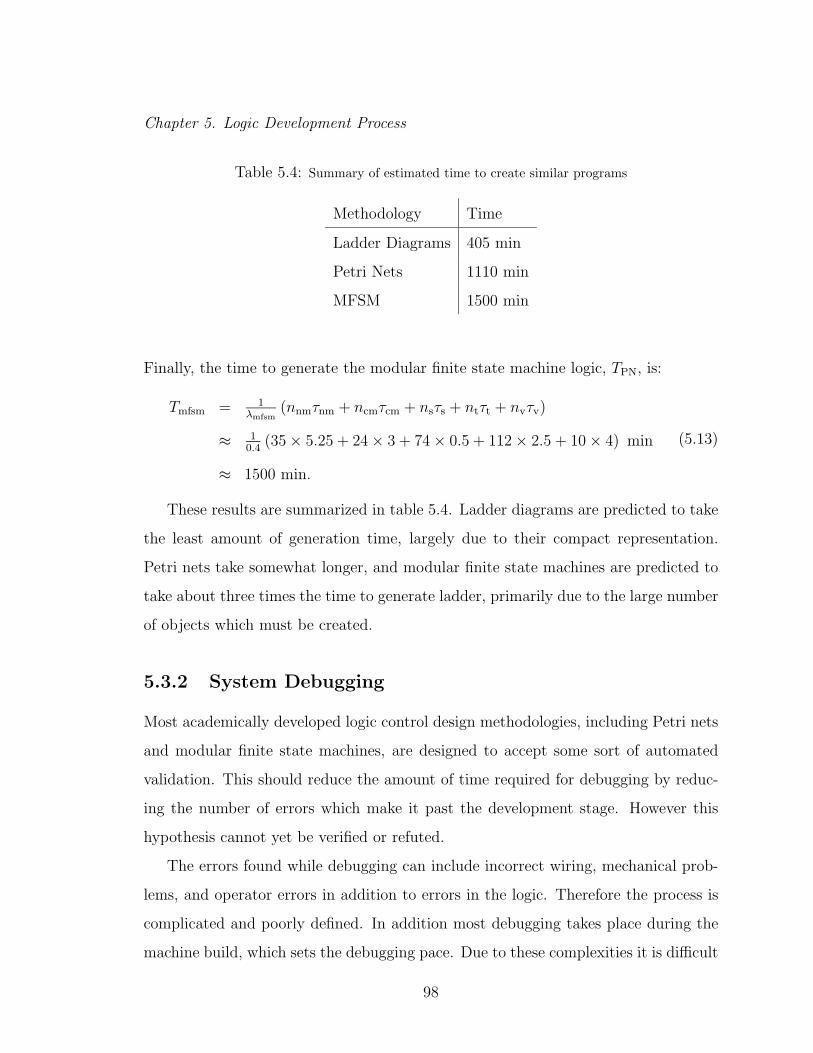
Chapter 5. Logic Development Process
Table 5.4: Summary of estimated time to create similar programs
Methodology Time
Ladder Diagrams 405 min
Petri Nets 1110 min
MFSM 1500 min
Finally, the time to generate the modular finite state machine logic, TPN, is:
Tmfsm = 1λmfsm
(nnmτnm + ncmτcm + nsτs + ntτt + nvτv)
≈ 10.4
(35 × 5.25 + 24 × 3 + 74 × 0.5 + 112 × 2.5 + 10 × 4) min
≈ 1500 min.
(5.13)
These results are summarized in table 5.4. Ladder diagrams are predicted to take
the least amount of generation time, largely due to their compact representation.
Petri nets take somewhat longer, and modular finite state machines are predicted to
take about three times the time to generate ladder, primarily due to the large number
of objects which must be created.
5.3.2 System Debugging
Most academically developed logic control design methodologies, including Petri nets
and modular finite state machines, are designed to accept some sort of automated
validation. This should reduce the amount of time required for debugging by reduc-
ing the number of errors which make it past the development stage. However this
hypothesis cannot yet be verified or refuted.
The errors found while debugging can include incorrect wiring, mechanical prob-
lems, and operator errors in addition to errors in the logic. Therefore the process is
complicated and poorly defined. In addition most debugging takes place during the
machine build, which sets the debugging pace. Due to these complexities it is difficult
98

Chapter 5. Logic Development Process
to quantify the potential time savings of a different logic control design methodology.
However, looking at the predicted debugging activities in figures 5.2, 5.4, and 5.6,
some comparisons can be made.
Ladder diagrams have a straightforward standard debug cycle: find suspect rung,
check its contacts. This rung either contains the error, or points to another problem,
which can be other rungs, suspect wiring, suspect sensors, or sometimes a memory bit
which was improperly set manually. This process is simple for most errors. However,
if problems span multiple rungs, or if a change in the sequential behavior is required,
then the debugger must adjust many seemingly independent rungs throughout the
program. In practice developers avoid such situations by restricting the specifica-
tions. That is, the expected machine behavior is restricted to those which are easily
implemented.
The nature of ladder diagrams is purely declarative. It is simple to verify certain
absolute restrictions on behavior. For example, the specification, “The part handling
shall advance only when all cutting tools are retracted” is easy to check. However
it is currently impossible to verify other, sequential restrictions. For example, the
specification, “Motion shall never start due to any action except a user-actuated
‘Start’ button” cannot be guaranteed.
The Petri net debug cycle is sequentially based. When an error is found, the
debugger must determine the sequence of transitions which lead to that error. The
Petri net must be searched since each output can be controlled from many places.
However, changing the behavior of the Petri net will often be easier, since the sequence
of operations can be read directly from the net.
The nature of Petri nets is purely sequential. It is simple to verify sequential
specifications, such as,“a machine cycle shall contain four operations in order, and
will only start when a when a user-actuated button is pressed”. However, declarative
requirements such as,“No movement shall occur when the emergency stop button is
pressed” can only be verified by exhaustively checking the reachability graph of the
99

Chapter 5. Logic Development Process
Table 5.5: Summary of logic control design methodology properties
Ladder Petri nets Modular FSM
Ease of learning Easy, already known Not widely known, difficult to learn
Program Style Output based Sequence based Function based
Debugging Output based Sequence based Module Based
Modularity Not modular Can be modular Very modular
Verification Not currently possi-
ble
Reachability verifi-
able
Modular communica-
tion verifiable
net.
The modular finite state machine debugging process starts with the incorrectly
behaving module, which must be checked sequentially like a Petri net. In many cases
the error must be tracked through multiple modules, requiring substantial memory
by the debugger. Changing the machine operation is relatively straightforward, since
the behavior of each module can be read directly from the states. In a well designed
system, this can be done both at a very high level (e.g. skip the second station for
some parts) or a very low level (e.g. turn off the spindle at the end of the machining
cycle).
The nature of modular finite state machines is both sequential and declarative.
The state machine inside each module is purely sequential, with all the benefits and
liabilities that implies. The structure of modules is more declarative. Users tend to
anthropomorphize modules and use phrases like,“This module ensures that the part
will always be in place”, which allows for some declarative thought.
A summary of the comparisons between the logic control design methodologies
considered is shown is table 5.5.
100
Chapter 6
Conclusions and Future Work
6.1 Summary of Contributions
There are three main results of this work: a better understanding of the methods
currently used in the automotive manufacturing industry to create logic, a method
of measuring the size and complexity of logic written using a variety of logic control
design methodologies, and a method of analyzing the process which would likely be
used if an alternative methodology was adopted.
6.1.1 Understanding current logic design methods
Chapter 3 described the current process of producing control logic for machining
systems using ladder diagrams. The process relies on both the reuse of logic from
previous projects and the expertise of the developers.
By observing the logic designers it was determined that designing logic for ma-
chining systems is substantially different than writing computer code, both in the
specification and in the people who will design and use the system. In addition, re-
cent academic developments in Discrete Event Systems are difficult to apply to the
problems of industrial logic control. Even methods which researchers design specifi-
101

Chapter 6. Conclusions and Future Work
cally for industrial logic design are difficult to apply, both due to the lack of support
for the methods, and the unsuitability of the methods to solve problems in this do-
main.
The primary results from the observational portion of this work are:
• The observed logic designers need to at least: determine acceptable machine
behavior, foresee potential error conditions, predict user behavior, and design
the logic needed for a machine. This is a greater range of responsibilities than
expected.
• Logic for one machine is generally copied directly from a previous project. How-
ever, copying logic generally involves manually re-typing everything due to in-
compatibilities in the development environments.
• Customers continue to ask for more features, and it is unlikely that this trend
will stop. Some of these features are extremely difficult to implement using exit-
ing methods. Such features include: detailed part tracking, more sophisticated
user interfaces, and greater diagnostic ability.
6.1.2 Measuring the Size and Complexity of Logic
The measurements introduced in chapter 4 provide two ways of comparing logic de-
veloped in different logic control design methodologies: direct, numerical measures,
which provide quantitative measurements of the size, modularity and connectedness
of logic regardless of which logic control design methodology is used to represent it;
and scenario-based measures, which provide a qualitative, user-oriented measure of
the effectiveness of a logic control design methodology at representing information.
Based on the measurements of logic samples, it is clear that the method of repre-
sentation affects the nature of the logic. The ladder representation is smaller, but is
very interconnected. The Petri net representations are the least interconnected, al-
though they are significantly larger. The modular finite state machine representation
102

Chapter 6. Conclusions and Future Work
is the most modular, although it is also the largest and is more interconnected than
the Petri net based solutions. In addition the difficulty of responding to the different
scenarios demonstrates that the method of solution varies significantly across scenar-
ios. These differences will affect the time and cost of developing and maintaining
logic.
6.1.3 Understanding Alternative Logic Control Design Method-
ologies
Chapter 5 develops a method of performing preliminary analysis of the effectiveness
of new or existing logic control design methodologies. This method includes approxi-
mating the time required to generate control logic as well as a qualitative comparison
of the debugging process implied by each methodology.
The method of comparing logic control design methodologies can be used very
early in their development, before integrated development environments are complete
and extensive user testing can be performed. It is based on a framework of the process
that is needed to create and debug logic. This comparison method provides objec-
tive measures that can be used to compare existing industrial logic control design
methodologies (such as ladder diagrams and flow charts) with more recently devel-
oped academic methods (such as Petri nets or state machines). This comparison
is demonstrated by comparing ladder diagrams, Petri nets and modular finite state
machines.
6.2 Discussion
Objective comparisons of logic control design methodologies are vital for ensuring that
the problems being addressed by research are valid solutions to the problems being
experienced in industry. In addition, there are substantial costs due to retraining
103
Chapter 6. Conclusions and Future Work
and transitional slowdowns which will be incurred during any transition. Before
widespread acceptance of a new methodology can be achieved, there must be some
assurance that the goal is worth the cost of transition. These comparison methods
may provide that assurance.
Based on these results, a widespread conversion to a new logic control design
methodology seems premature at this point. Ladder diagrams appear to be a more
compact representation, leading to faster development times. They also appear ade-
quate to the current needs of industry.
However, current logic control design methodologies may have been pushed as far
as possible. During research discussed in chapter 3 some tasks were observed that
appeared to be beyond current capabilities. These tasks included certain additions to
the operator console, such as full control of the machine from the console, a console
that can be virtually moved to different stations, or operator buttons that “grey out”
when a particular action is not possible. Features which are possible but difficult
include substantial diagnostics and detailed part tracking. For example, currently it
is difficult to create a diagnostic which will intelligently guess what relay has failed,
rather than producing a more generalized fault message. Even generating diagnostic
text messages is difficult, since every message used must be entered into memory
and subsequently accessed via its memory location. Detailed part tracking includes
tracking information about every action on every part, which is common in some
assembly operations, but difficult to accomplish using ladder diagrams.
There are a number of developments which could make alternative methodologies
more attractive. As automatic verification methods become better understood, it
may be possible to reduce the estimated debugging effort significantly. If a compre-
hensive library of ready-to-use, zero-modification modules can be developed, then the
estimated development time would decrease. Such modules are not possible when
using a global name space, as with most ladder editors. Finally, a method of creat-
ing well-written ladder diagrams automatically from Petri net or modular finite state
104

Chapter 6. Conclusions and Future Work
machine specifications would reduce the cost of transition, since shop floor personnel
would not need to be retrained.
6.3 Future Work
There are many areas of possible future work based on this research. Additional
data collection, both on the development process and studies of existing logic would
validate and add to the results of this work. In addition, methods of reliably predict-
ing the size of logic needed to control a machine using various logic control design
methodologies are needed to properly understand the development process of each.
Finally, a method to generate traditional, human readable ladder diagrams would
greatly ease the transition to any future methodology.
6.3.1 Additional Data Collection
First, measurements of logic samples which are larger and contain more exception
handling will provide more insight into the nature of each logic control design method-
ology. The samples presented in this dissertation control a system with 15 inputs and
15 outputs, and contain no exception handling. Industrial scale systems can easily
contain 10,000 I/O points, and must handle many error conditions correctly.
In addition, additional observational studies (such as chapter 3) will fill out the
space of problems which are being solved using PLC programming. Of interest is how
much truly new design is being done. This will determine if the most useful advances
will be faster reuse of existing logic, or easier design of new logic.
These studies can be used to construct more detailed models of the logic generation
process. More detailed models would allow for better estimates of the time required
for certain subtasks, and a more detailed view of the the tasks involved in memory
management or project coordination. Variations between different groups of designers
would also be interesting.
105

Chapter 6. Conclusions and Future Work
6.3.2 A priori size estimation
Studies and measurements of more existing logic solutions, especially large samples,
will help future researchers predict the size and structure of logic needed to solve a
particular specification. Logic size is one of the most important factors when consid-
ering development time.
Currently there is no method of estimating the size of a piece of logic a priori.
There are have a limited number of empirical examples, which have been used for
our studies to date. One method of forming an a priori estimate would be to find
more real examples, and determine the trends in size. For example, the size of a
ladder program is linear with the number of outputs, with the complexity of the
program presenting a complicating factor. This is usually a known quantity during
the design stage. However, the size of a Petri net is probably dependent only on the
complexity of the specifications, and predicting the “complexity” presents issues of
its own. The size of a modular finite state machine solution seems linear with the
number of modules, which is determined both by the complexity of the specification,
and the number of components.
6.3.3 Automatically Generating Ladder Diagrams
If high quality ladder diagrams could be generated from specifications written in other
methodologies, those methodologies would be much more useful. Arguing by analogy:
CAD/CAM packages routinely generate the G-code required to manufacture a certain
part. Using this primitive code, very sophisticated programs can communicate effec-
tively with older machines. Just as important, the operators of those machines are
given something that they understand, and can modify if needed. If human-readable,
traditionally formatted ladder diagrams could be generated from Petri nets, modular
finite state machines, or any other methodology, then the cost of retraining end-
user personnel would be eliminated and industrial quality hardware would be readily
106

Chapter 6. Conclusions and Future Work
available.
Previous efforts to translate Petri nets or state machines to ladder logic have
generally relied upon “token passing logic”. Using this method each transition is
used to create one rung. These rungs use latch/unlatch coils to managed the “states”
of the system. While this is perfectly intuitive to most academicians, this is not how
ladder logic is written by humans. In fact, current designers go out of their way to
avoid the use of latched coils, because they can lead to unexpected operation when the
machine is started up. (Latch states must be maintained during a power shutdown.)
To generate properly styled ladder diagrams a unique abstraction tool is needed.
The number of states required must be minimized, and as many as possible should
be used as outputs (thus minimizing the memory required). Most states need to be
maintained by “sealed circuits” rather than latch coils, to allow for proper power
down behavior. (A sealed circuit is one whose output is read as an input, allowing
for state to be maintained. Figures 1.1, 2.3, and 4.2 are examples of sealed circuits.)
A typical human-generated ladder diagram project only has one main internal
state for each station, called “full-depth”. Typical operation attempts to push all the
items toward the part (using interlocks to create the correct ordering) until the full
depth of cut is reached. Then the “full depth” bit is set, and the logic drives all the
parts back, until eventually the “full-depth” bit is unset. Additional bits are used to
maintain fault conditions.
An alternative method is known as “steps programming”. (Note the similarity
the the term “step” from SFCs, where a “place” is referred to as a “step”.) In this
style of programming, multiple bits are created which represent the various steps of
the machining cycle. At each step the machine is driven towards the next, until the
full cycle has been completed. Engineers at Lamb consider steps programming to be
needlessly complex and error prone.
“Full-depth” programming can be considered as a simple case of “steps program-
ming”, with only one step defined.
107

Chapter 6. Conclusions and Future Work
A method of creating logic which conformed to a more human-readable style would
allow the programmers who wished to use more advanced tools, while allowing their
work to be effectively used by existing personnel.
108

Bibliography
[1] S. Balemi. Input/output discrete event processes and system modeling. In DiscreteEvent Systems: Modeling and Control, pages 15–27. Birkhauser, 1992.
[2] R. Brooks, Rockwell Software. Personal communication.
[3] S. K. Card, W. K. English, and B. J. Burr. Evaluation of a mouse, rate-controlledisometric joystick, step keys and text keys for text selection on a CRT. Ergonomics,21:601 – 613, 1978.
[4] S. K. Card, T. P. Moran, and A. Newell. The keystroke-level model for user performancetime with interactive systems. Communications of the ACM, 23(7):396 – 410, July 1980.
[5] S. K. Card, T. P. Moran, and A. Newell. The Psychology of Human-Computer Inter-action. Lawrence Erlbaum Associates, 1983.
[6] C. G. Cassandras and S. Lafortune. Introduction to Discrete Event Systems. KluwerAacdemic Publishers, 1999.
[7] M. S. Castor and D. L. Hurd. A case for ladder logic. Control Engineering, pages152–166, November 1988.
[8] S.D. Conte, H.E. Dunsmore, and V.Y. Shen. Software Engineering Metrics and Models.The Benamin/Cummings Publishing Company Inc., 1986.
[9] E. W. Endsley, M. R. Lucas, and D. M. Tilbury. Software tools for verification ofmodular FSM based logic control for use in reconfigurable machining systems. Japan–U.S.A. Symposium on Flexible Automation, 2000.
[10] PLC graphical languages speed process design and startup. Engineering and MiningJournal, 199(8), August 1998.
[11] K. Feldman, A. W. Colombo, C. Schur, and T. Stockel. Specification, design, andimplementation of logic controllers based on colored Petri net models and the standardIEC 1131 part I: Specification and design. IEEE Transactions on Control SystemsTechnology, 7(6):657–665, November 1999.
[12] A R. Feuer and N. H. Gehani. A methodology for comparing programming languages.In A. R. Feuer and N. H. Gehani, editors, Comparing and Assessing ProgrammingLanguages: Ada, C, and Pascal, pages 197–208. Prentice-Hall, Inc., 1987.
109

BIBLIOGRAPHY
[13] P. M. Fitts and J. R. Peterson. Information capacity of discrete motor responses.Journal of Experimental Psychology, 67(2):103–112, February 1964.
[14] G. Frey. SIPN, hierarchical SIPN, and extensions. Technical report, Universitat Kaiser-slautern, Germany, 2001. http://www.eit.uni-kl.de/litz/members/frey/PDF/I19.pdf.
[15] G. Frey and L. Litz. A measure for transparency in net based control algorithms. InIEEE International Conference on Systems, Man, and Cybernetics ‘Human Commu-nication and Cybernetics’, pages 887–892, 1999.
[16] G. Frey and L. Litz. Transparency analysis of Petri net based logic controllers — ameasure for software quality in automation. In Proceedings of the American ControlConference, pages 3182–3186, 2000.
[17] D. J. Gilmore and T. R. Green. Comprehension and recall of miniature programs.International Journal of Man-Machine Studies, 21:31–48, 1984.
[18] C. Gollapudi and D. M. Tilbury. Logic control design and implementation for a machin-ing line testbed using Petri nets. In Proceedings of the ASME International MechanicalEngineering Congress and Exposition (Dynamic Systems and Control Division), NewYork, November 2001.
[19] J. Good. VPLs and novice comprehension: How do different languages compare? InIEEE Symposium on Visual Languages, pages 262–269, 1999.
[20] T. R. Green and M. Petre. Usability analysis of visual programming environments:A ‘cognitive dimensions’ framework. Journal of Visual Languages and Computing,7:131–174, 1996.
[21] M. H. Halstead. Elements of software science. Elsevier, 1977.
[22] D. Harel and A. Naamad. The statemate semantics of statecharts. ACM Transactionson Software Engineering and Methodology, 5(4):293 – 333, 1996.
[23] L. Holloway. Spectool, 2000. http://www.crms.engr.uky.edu/pages/spectool/.
[24] L. E. Holloway, X. Guan, R. Sundaravadivelu, and J. Ashley, Jr. Automated synthesisand composition of taskblocks for control of manufacturing systems. IEEE Transac-tions on Systems, Man, and Cybernetics—Part B: Cybernetics, 30(5), October 2000.
[25] D. Johnson. Nano devices lead assault on traditional PLC applications. Control Engi-neering, pages 43–44, August 2002.
[26] B. S. Kang and K. H. Cho. Design of PLCs for automated industrial systems basedon discrete event models. IEEE International Symposium on Industrial Electronics,8:1431–1434, 2001.
[27] D. E. Kieras. Towards a practical GOMS model methodology for user interface de-sign. In Handbook of Human-Computer Interaction, chapter 7, pages 135–157. ElsevierScience Publishers B.V, 1988.
110

BIBLIOGRAPHY
[28] D. E. Kieras. Task analysis and the design of functionality. In A. B. Tucker, editor,The Computer Science and Engineering Handbook. CRC Press, 1997.
[29] Tim King Electronics Inc. http://www.phoenix.org/tking/index.shtml.
[30] S. Klein and G. Frey. Control of a flexible manufacturing system using sipn. Reportsof the institute of automatic control i23/2002, University of Kaiserslautern, Germany,July 2002. http://www.eit.uni-kl.de/litz/members/frey/PDF/I23.pdf.
[31] S. Klein, X. Weng, G. Frey, J. Lesage, and L. Litz. Controller design for an FMSusing signal interpreted Petri nets and SFC: Validation of both descriptions via modelchecking. In Proceedings of the American Control Conference, pages 4141–4146, 2002.
[32] A. Krigman. Relay ladder diagrams: We love them, we love them not. InTech, pages39–44, October 1985.
[33] J. S. Lee and P. L. Hsu. A PLC-based design for the sequence fontroller in discrete eventsystems. In IEEE International Conference on Control Applications, pages 929–934,September 2000.
[34] J. S. Lee and P. L. Hsu. A new approach to evaluate ladder diagrams and Petri netsvia the if-then transformation. In IEEE Conference on Systems, Man and Cybernetics,pages 2711–2716, Tucson, AZ, 2001.
[35] R. W. Lewis. Programming Industrial Control Systems Using IEC 1131-3 RevisedEdition. The Institution of Electrical Engineers, 1998.
[36] R. W. Lewis. Modeling control systems using IEC 61499. The Institution of ElectricalEngineers, London, 2001.
[37] M. R. Lucas, E. W. Endsley, and D. M. Tilbury. Coordinated logic control for re-configurable machine tools. In Proceedings of the American Control Conference, pages2107–2113, 1999.
[38] M. R. Lucas and D. M. Tilbury. Quantative and qualitative comparisons of PLCprograms for a small testbed with a focus on human issues. In Proceedings of theAmerican Control Conference, May 2002.
[39] M. R. Lucas and D. M. Tilbury. Comparing industrial design methods used in the auto-motive industry. In IEEE International Conference on Systems, Man and Cybernetics,October 2003. Accepted for publication.
[40] M. R. Lucas and D. M. Tilbury. A comparison of logic control design methodologiesused or proposed for use in the automotive industry. IEEE Transactions on IndustrialElectronics, 2003. Submitted for publication.
[41] M. R. Lucas and D. M. Tilbury. Methods of measuring the size and complexity ofPLC programs in different logic control design methodologies. Internation Journal ofAdvanced Manufacturing Technology, 2003. Submitted for publication.
111
BIBLIOGRAPHY
[42] M. R. Lucas and D. M. Tilbury. A study of current logic design practices inthe automotive industry. International Journal of Human-Computer Studies, 2003.Accepted for publication, available at http://www-personal.engin.umich.edu/ mrlu-cas/Papers/LT03 IJHCS submitted.pdf.
[43] PLCs speak many tongues. Machine Design, 67(8):158, April 1995.
[44] P. Marti. Structured task analysis in complex domains. Ergonomics, 41(11):1664 –1677, 1998.
[45] M. Minas and G. Frey. Visual PLC-programming using signal interpreted Petri nets.In Proceedings of the American Control Conference, pages 5019–5024, 2002.
[46] T. G. Moher, D. C. Mak, B. Blumenthal, and L. M. Leventhal. Comparing the com-prehensibility of textual and graphical programs: The case for Petri nets. In C. R.Cook, J. C. Scholtz, and J. C. Spohrer, editors, Empirical Studies of Programmers:Fifth Workshop. Ablex Publishing Group, 1990.
[47] R. H. Morihara. State-based ladder logic programming. In Proceedings of the Engi-neering Society of Detroit, pages 157–167, Ann Arbor, MI, 1994.
[48] Nematron logic control software. http://www.nematron.com/OpenControl/.
[49] J. R. Olson and G. M. Olson. The growth of cognitive modeling in human-computerinteraction since GOMS. Human-Computer Interaction, 5:221 – 265, 1990.
[50] E. Park, D. M. Tilbury, and P. P. Khargonekar. Modular logic controller for machiningsystems: Formal representation and performance analysis using Petri nets. IEEETransactions on Robotics and Automation, 15(6):1046–1061, December 1999.
[51] E. Park, D. M. Tilbury, and P. P. Khargonekar. A modeling and analysis methodologyfor modular logic controllers of machining systems using Petri net formalism. IEEETransactions on Systems, Man, and Cybernetics—Part C: Applications and Reviews,31(2):168–188, 2001.
[52] S. Peng and M. Zhou. Conversion between ladder diagrams and PNs in discrete-eventcontrol design — a survey. In IEEE conference on Systems, Man and Cybernetics,pages 2682–2687, 2001.
[53] N. Pennington. Comprehension strategies in programming. In G. M. Olsen, S. Shepard,and E. Soloway, editors, Empirical Studies of Programmers: Second Workshop. AblexPublishing Group, 1987.
[54] N. Pennington. Stimulus structures and mental representations in expert comprehen-sion of computer programs. Cognitive Psychology, 19:295–341, 1987.
[55] J. R. Pollard. Ladder logic remains the PLC language of choice. Control Engineering,pages 77–79, April 1999.
112

BIBLIOGRAPHY
[56] D. Ponizil. Back to basics: The essentials of structured PLC. Control Engineering, 48,September 2001.
[57] P. J. G. Ramadge and W. M. Wonham. Supervisory control of a class of discrete eventprocesses. SIAM Journal of Control and Optimization, pages 206 – 230, January 1987.
[58] P. J. G. Ramadge and W. M. Wonham. The control of discrete event systems. Pro-ceedings of the IEEE, 77(1):81–98, January 1989.
[59] R. Roberts. Zone Logic: A Unique Method of Practical Artificial Intelligence. Compute!Books, 1989.
[60] S. S. Shah, E. W. Endsley, M. R. Lucas, and D. M. Tilbury. Reconfigurable logiccontrol using modular finite state machines: Design, verification, implementation, andintegrated error handling. In Proceedings of the American Control Conference, 2002.
[61] A. Shepherd. HTA as a framework for task analysis. Ergonomics, 41(11):1537–1552,1998.
[62] D. M. Tilbury. Logic control testbed, 2001. http://www-personal.engin.umich.edu/˜tilbury/testbed.
[63] M. Uzam, A. H. Jones, and I. Yucel. Using a Petri-net-based approach for the real-timesupervisory control of an experimental manufacturing system. International Journalof Advanced Manufacturing Technology, 16:498–515, 2000.
[64] V. VanDoren. Designing PLC-based control without ladder logic. Control Engineering,page 110, June 1996.
[65] K. Vankatesh, M. Zhou, and R. J. Caudill. Comparing ladder logic diagrams and Petrinets for sequence controller design through a discrete manufacturing system. IEEETransactions on Industrial Electronics, 41(6):611–619, December 1994.
[66] S. Wiedenbeck, V. Ramalingam, S. Sarasamma, and C. L. Corritore. A comparison ofthe comprehension of object-oriented and procedural programs by novice programmers.Interacting with Computers, 11:255–282, 1999.
[67] N. Wirth. Programming langages: What to demand and how to assess them. In A. R.Feuer and N. H. Gehani, editors, Comparing and Assessing Programming Languages:Ada, C, and Pascal, pages 24–261. Prentice-Hall, Inc., 1987.
[68] S. N. Woodfield, V. Y. Shen, and H. E. Dunsmore. A study of several metrics forprogramming effort. The Journal of Systems and Software, 2(2):97–103, 1981.
113