understand your design - prace training portal: events 1 - agenda introduction motivation for...
TRANSCRIPT
Understand your Design
- 1 -
Agenda
Introduction
Motivation for parametric variations
Parametric workflow in ANSYS
Manual variation
Systematic variation using optiSLang for ANSYS
Typical Questions
Efficient performance of extensive design variation
Understand your Design
Motivation for parametric variation
PRACE Autumn School 2013 - Industry Oriented HPC Simulations, September 21-27,
University of Ljubljana, Faculty of Mechanical Engineering, Ljubljana, Slovenia
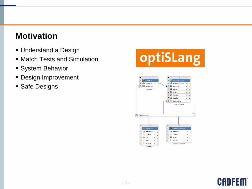
Motivation
- 1 -
Understand a Design
Match Tests and Simulation
System Behavior
Design Improvement
Safe Designs
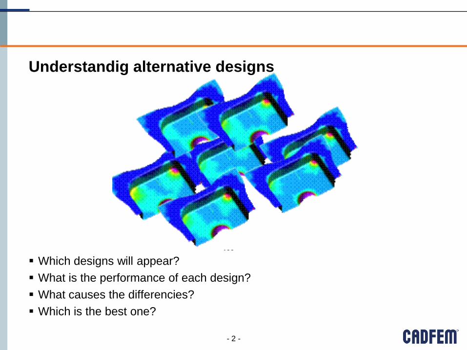
Understandig alternative designs
- 2 -
Which designs will appear?
What is the performance of each design?
What causes the differencies?
Which is the best one?
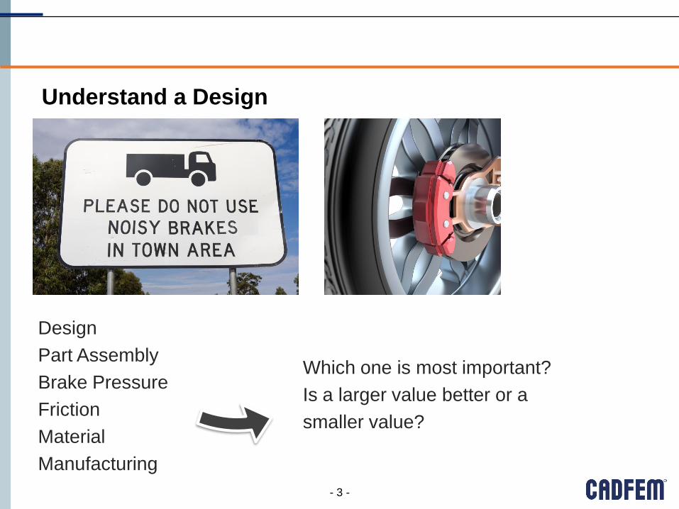
Understand a Design
- 3 -
Design
Part Assembly
Brake Pressure
Friction
Material
Manufacturing
Which one is most important?
Is a larger value better or a
smaller value?
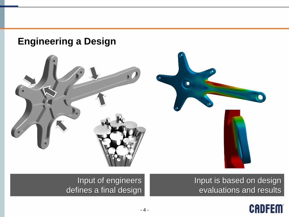
Engineering a Design
- 4 -
Input of engineers
defines a final design
Input is based on design
evaluations and results
Benefits of a parametric design variation
- 5 -
Get the most significant parameters.
Check correlations.
Estimate numerical noise.
Determine difficulties in extracting results.
Estimate numerical stability.
Check your geometrical validity.
Check potential design improvement.
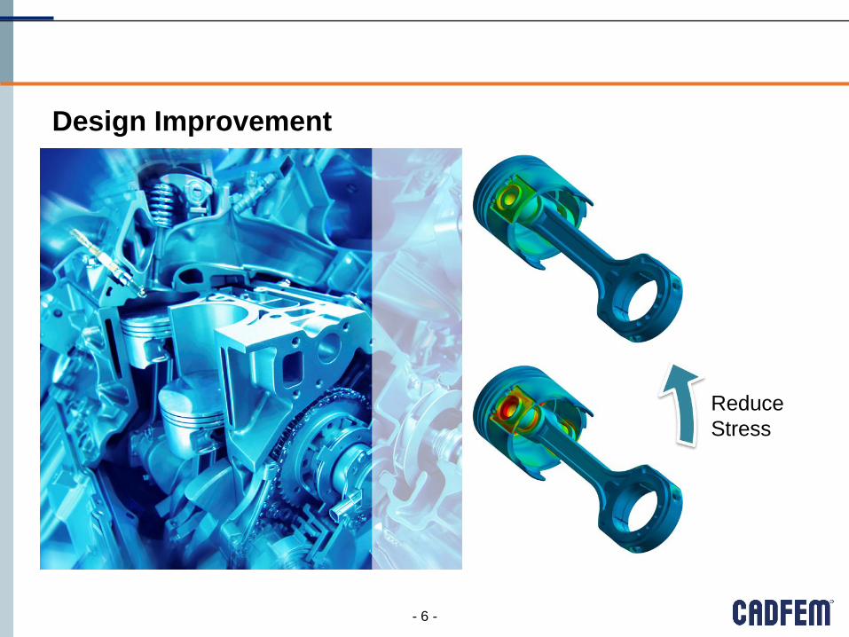
Design Improvement
- 6 -
Reduce
Stress
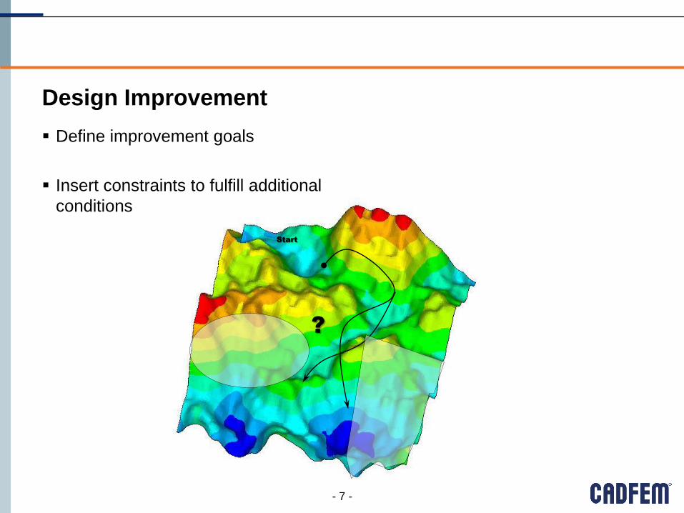
Design Improvement
- 7 -
Define improvement goals
Insert constraints to fulfill additional
conditions
?
Start
- 8 -
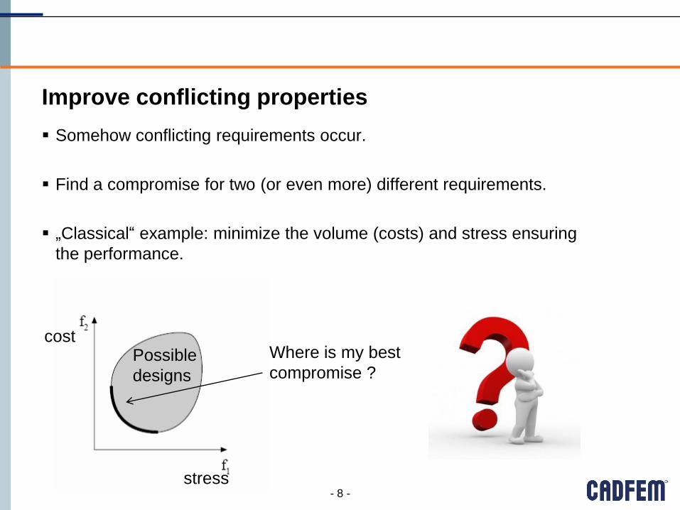
Improve conflicting properties
Somehow conflicting requirements occur.
Find a compromise for two (or even more) different requirements.
„Classical“ example: minimize the volume (costs) and stress ensuring
the performance.
Where is my best
compromise ?
cost
stress
Possible
designs
- 9 -
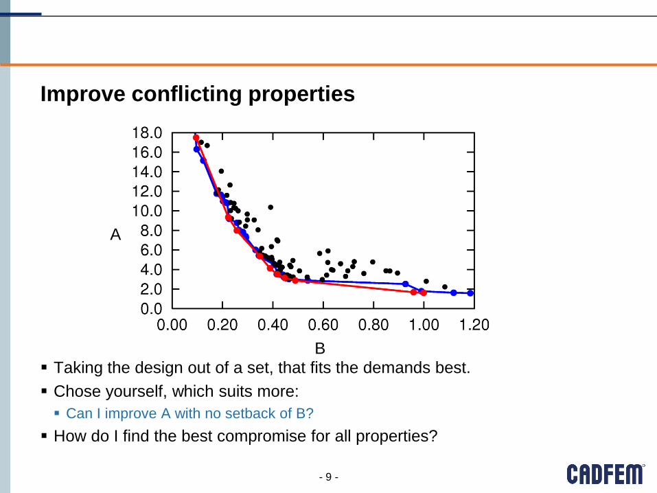
Improve conflicting properties
Taking the design out of a set, that fits the demands best.
Chose yourself, which suits more:
Can I improve A with no setback of B?
How do I find the best compromise for all properties?
A
B
- 10 -
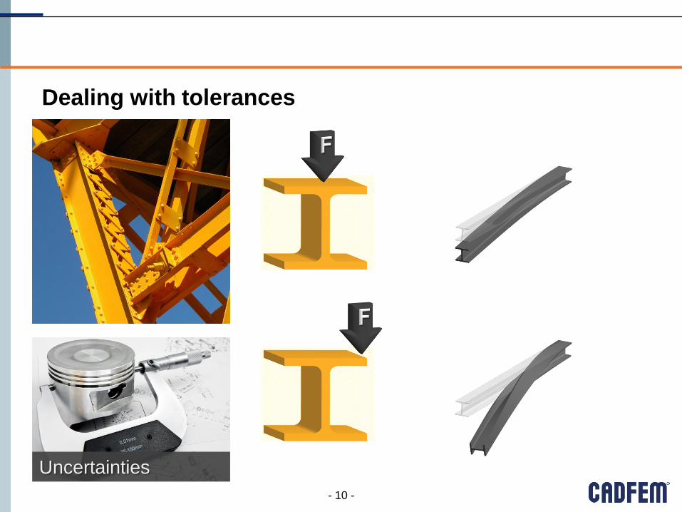
Dealing with tolerances
Uncertainties
- 11 -
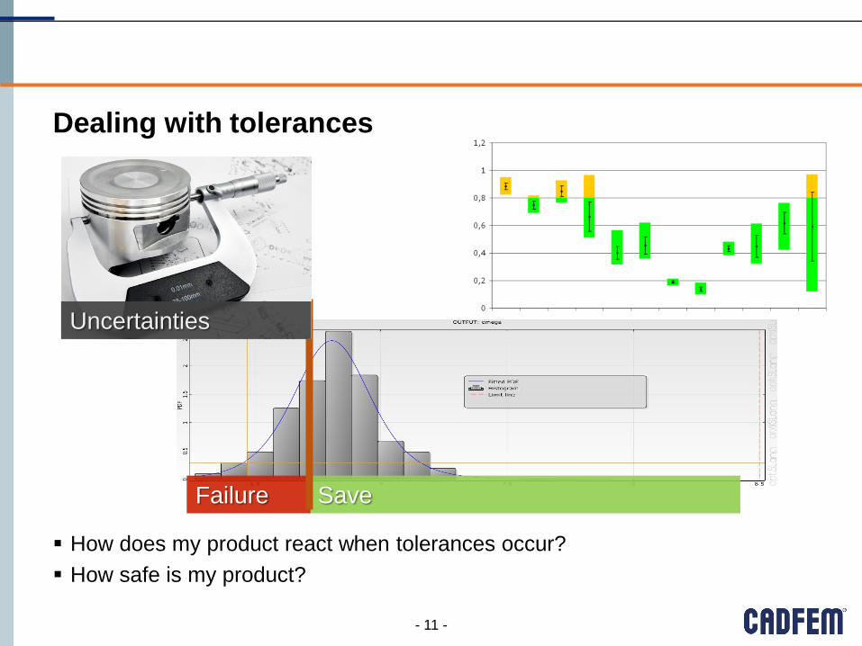
Dealing with tolerances
How does my product react when tolerances occur?
How safe is my product?
Save Failure
Uncertainties
Parameter Adjustment
Test
Simulation
- 12 -
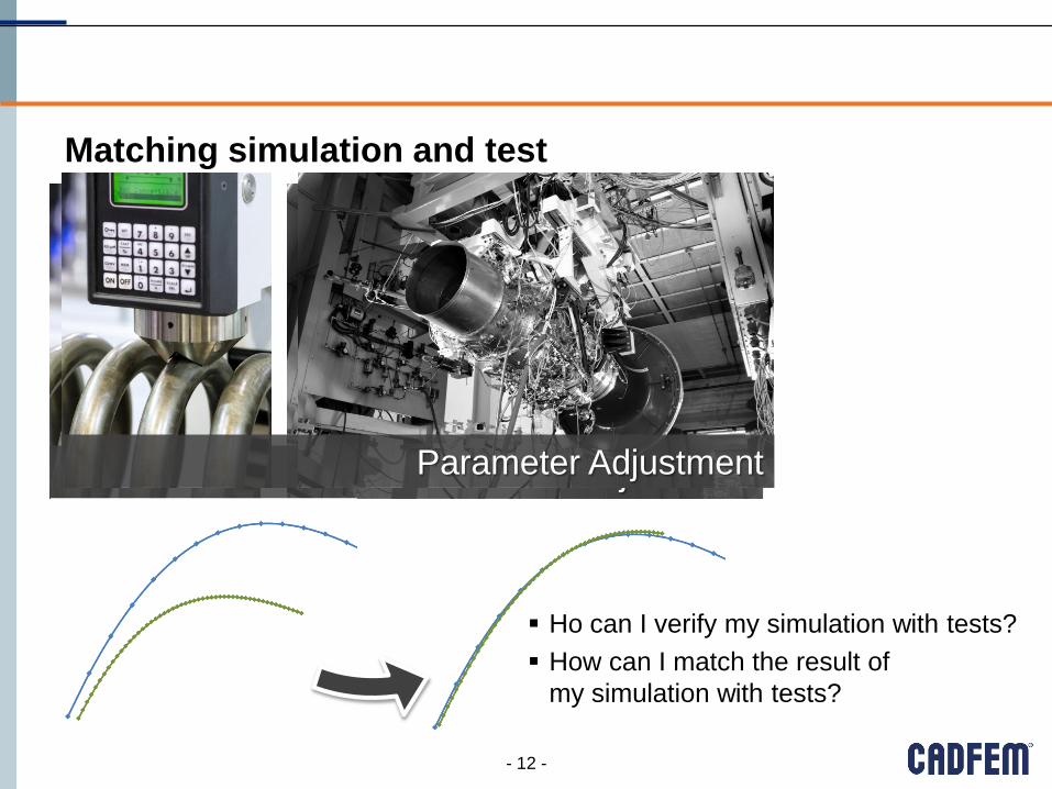
Matching simulation and test
Ho can I verify my simulation with tests?
How can I match the result of
my simulation with tests?
Parameter Adjustment
- 13 -
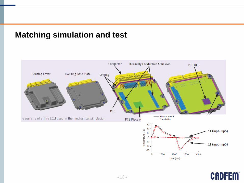
Matching simulation and test
- 14 -
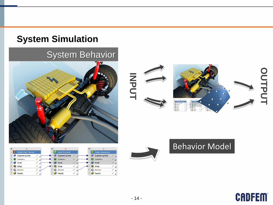
System Simulation
Behavior Model
OU
TP
UT
System Behavior
INP
UT
- 15 -
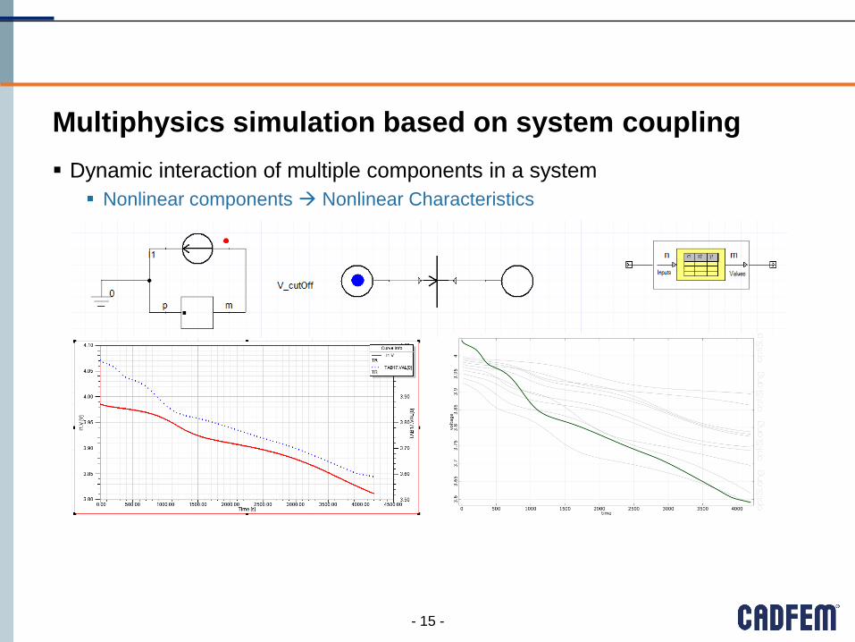
Multiphysics simulation based on system coupling
Dynamic interaction of multiple components in a system
Nonlinear components Nonlinear Characteristics
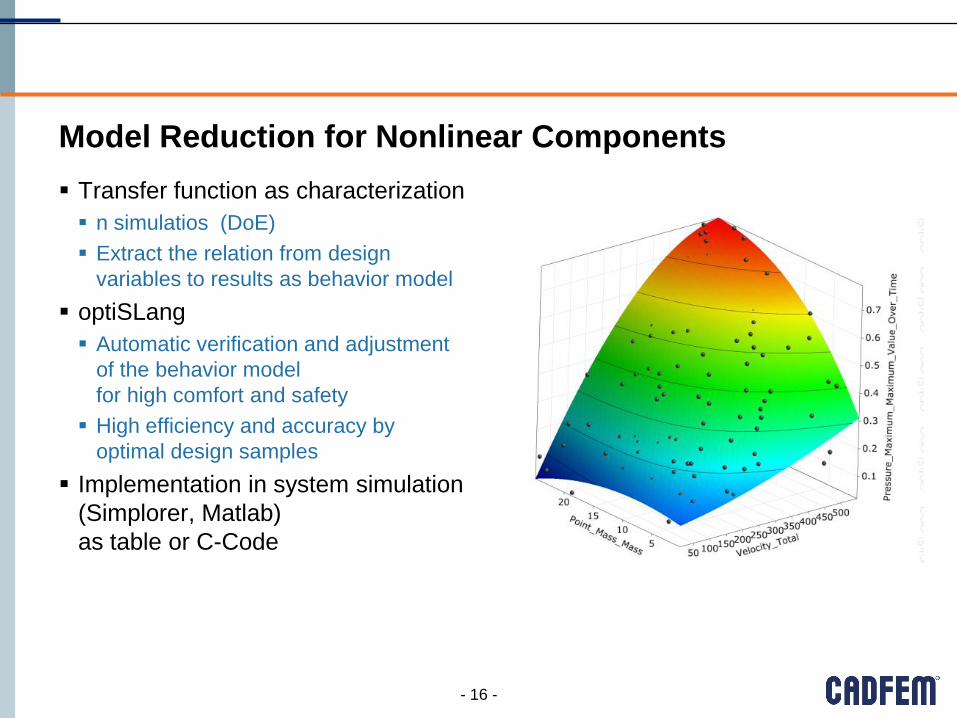
Model Reduction for Nonlinear Components
Transfer function as characterization
n simulatios (DoE)
Extract the relation from design
variables to results as behavior model
optiSLang
Automatic verification and adjustment
of the behavior model
for high comfort and safety
High efficiency and accuracy by
optimal design samples
Implementation in system simulation
(Simplorer, Matlab)
as table or C-Code
- 16 -
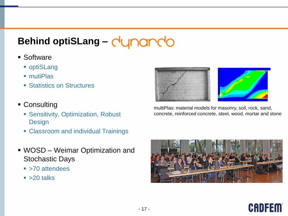
Behind optiSLang – Dynardo G
Software
optiSLang
mutiPlas
Statistics on Structures
Consulting
Sensitivity, Optimization, Robust
Design
Classroom and individual Trainings
WOSD – Weimar Optimization and
Stochastic Days
>70 attendees
>20 talks
- 17 -
multiPlas: material models for masonry, soil, rock, sand,
concrete, reinforced concrete, steel, wood, mortar and stone
Understand Your Design Parametric Workflow in ANSYS
PRACE Autumn School 2013 - Industry Oriented HPC Simulations, September 21-27,
University of Ljubljana, Faculty of Mechanical Engineering, Ljubljana, Slovenia
- 1 -
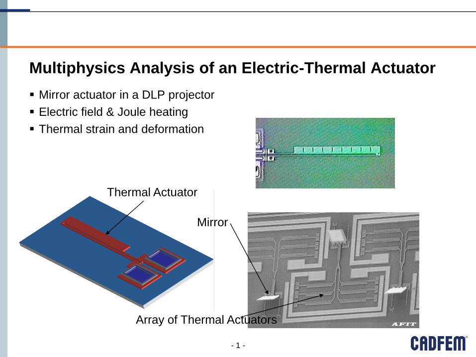
Multiphysics Analysis of an Electric-Thermal Actuator
Mirror actuator in a DLP projector
Electric field & Joule heating
Thermal strain and deformation
Thermal Actuator
Mirror
Array of Thermal Actuators
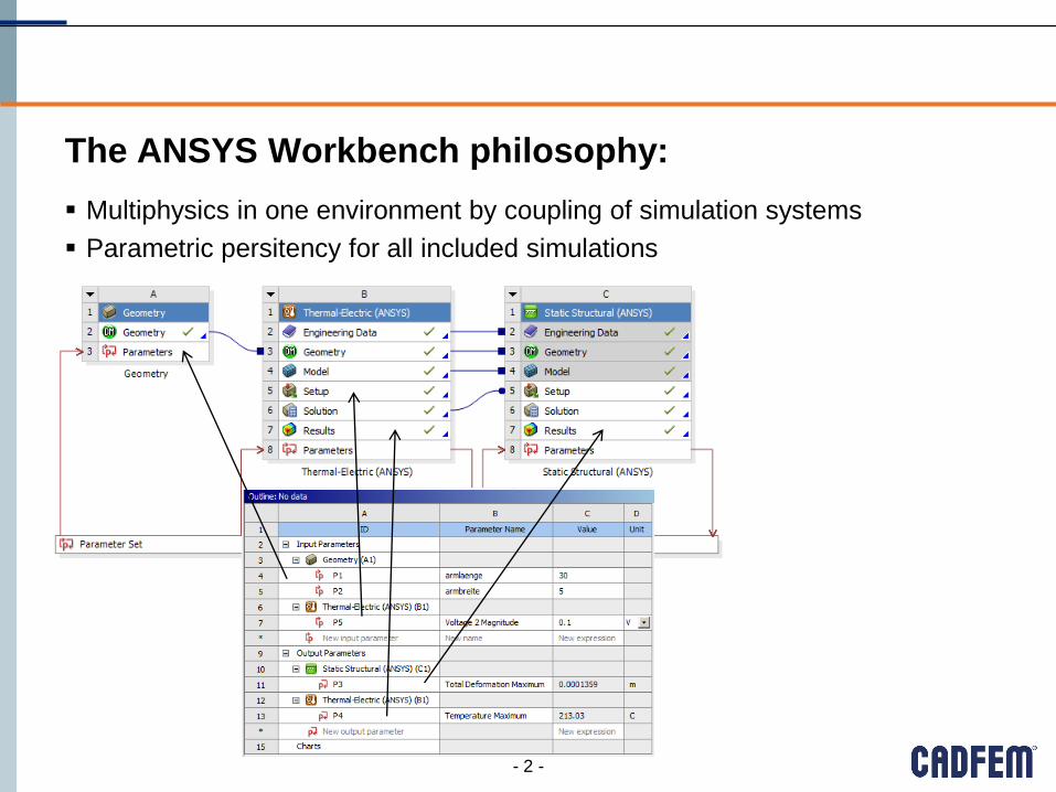
Multiphysics in one environment by coupling of simulation systems
Parametric persitency for all included simulations
- 2 -
The ANSYS Workbench philosophy:
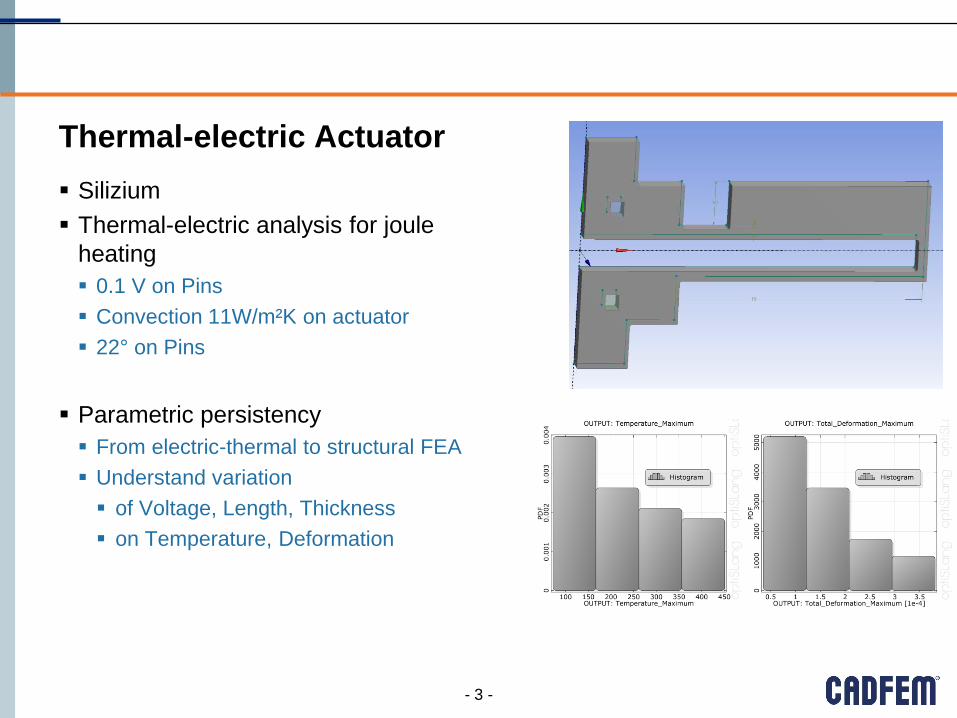
Thermal-electric Actuator
- 3 -
Silizium
Thermal-electric analysis for joule
heating
0.1 V on Pins
Convection 11W/m²K on actuator
22° on Pins
Parametric persistency
From electric-thermal to structural FEA
Understand variation
of Voltage, Length, Thickness
on Temperature, Deformation
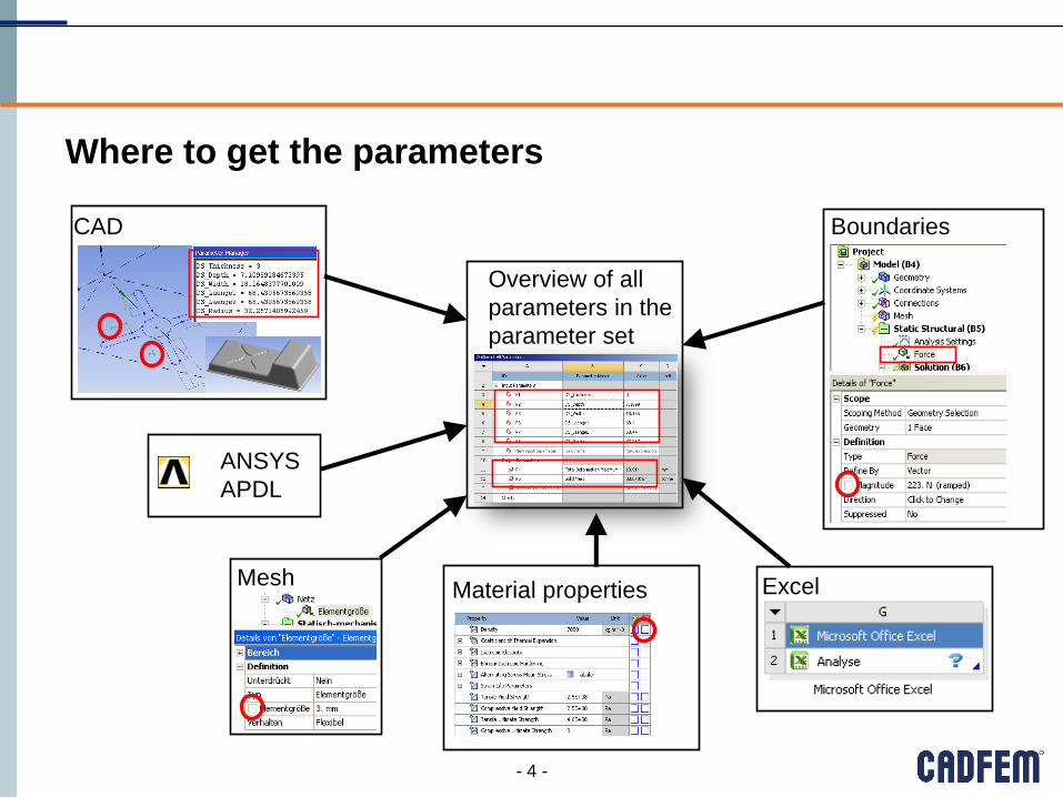
CAD
Material properties
Boundaries
ANSYS
APDL
Excel Mesh
Overview of all
parameters in the
parameter set
- 4 -
Where to get the parameters
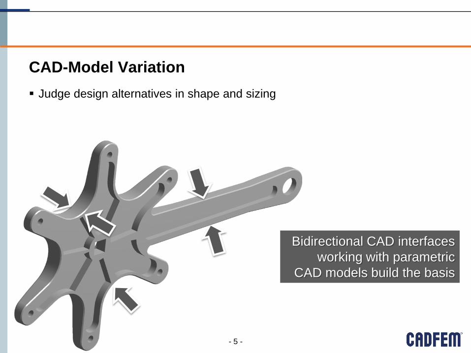
CAD-Model Variation
Judge design alternatives in shape and sizing
- 5 -
Bidirectional CAD interfaces
working with parametric
CAD models build the basis
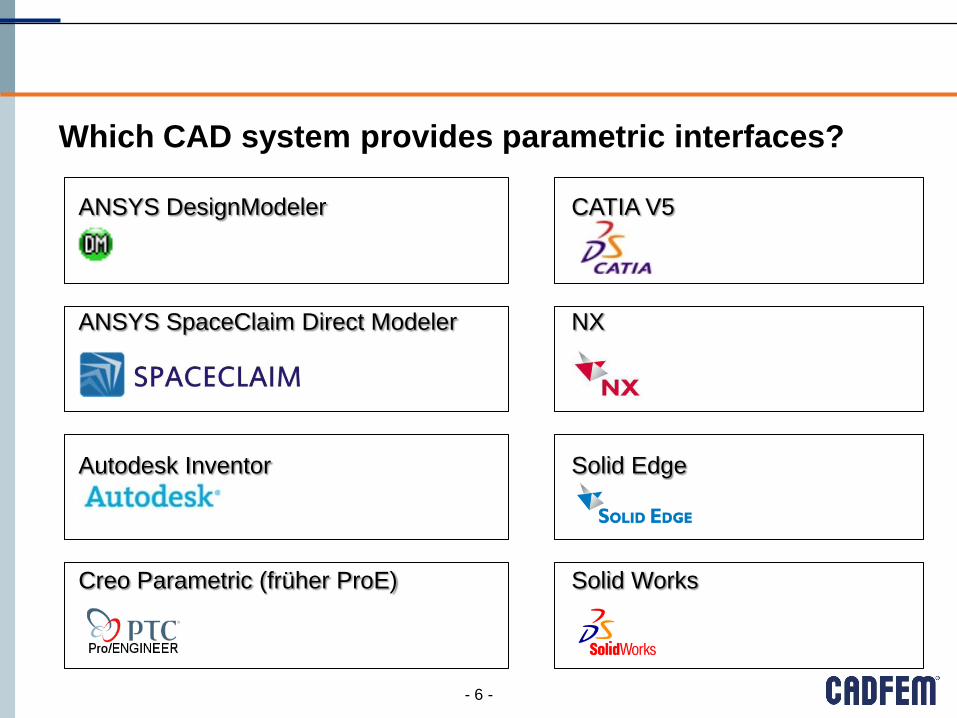
ANSYS DesignModeler
ANSYS SpaceClaim Direct Modeler
Autodesk Inventor
Creo Parametric (früher ProE)
CATIA V5
NX
Solid Edge
Solid Works
- 6 -
Which CAD system provides parametric interfaces?
- 7 -
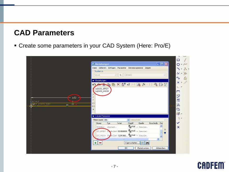
CAD Parameters
Create some parameters in your CAD System (Here: Pro/E)
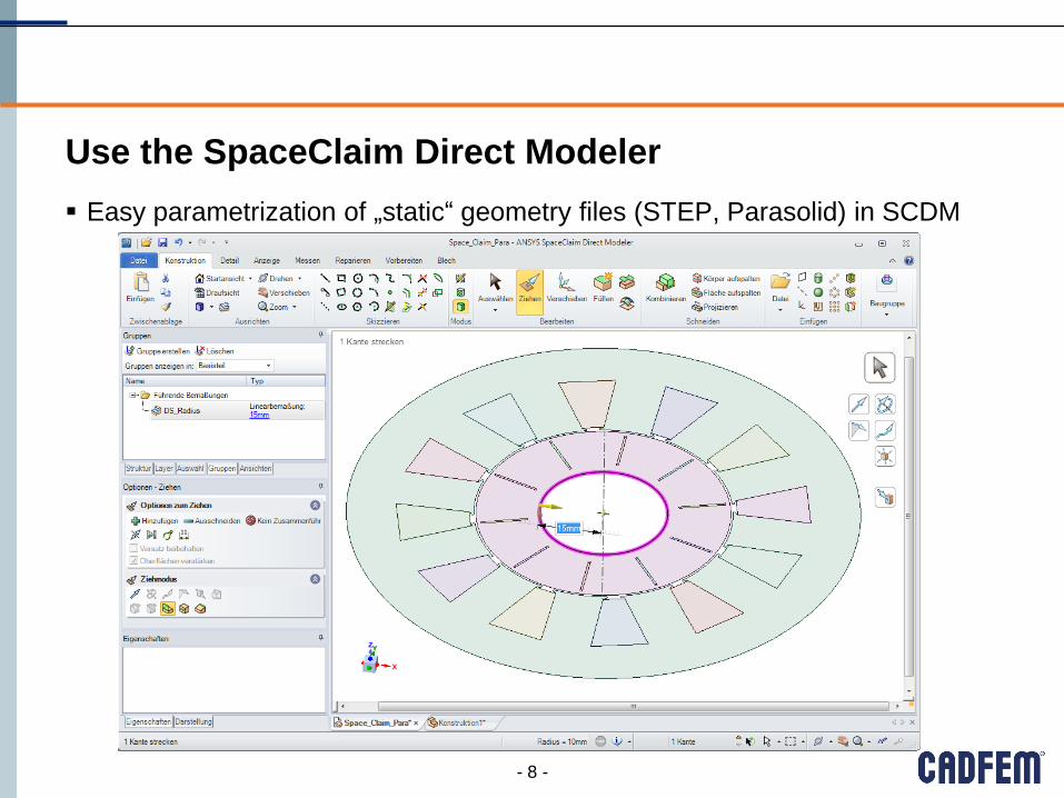
Use the SpaceClaim Direct Modeler
Easy parametrization of „static“ geometry files (STEP, Parasolid) in SCDM
- 8 -
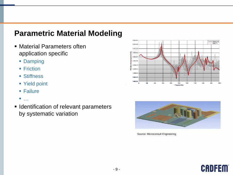
Parametric Material Modeling
- 9 -
Material Parameters often
application specific
Damping
Friction
Stiffness
Yield point
Failure
…
Identification of relevant parameters
by systematic variation
Source: Microconsult Engineering
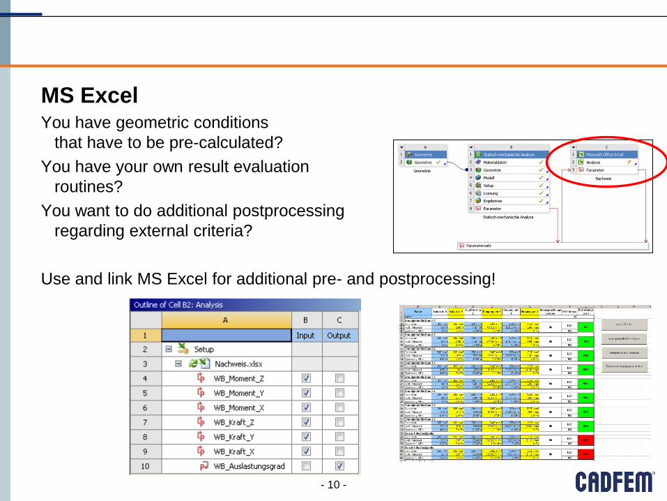
MS Excel
- 10 -
You have geometric conditions
that have to be pre-calculated?
You have your own result evaluation
routines?
You want to do additional postprocessing
regarding external criteria?
Use and link MS Excel for additional pre- and postprocessing!
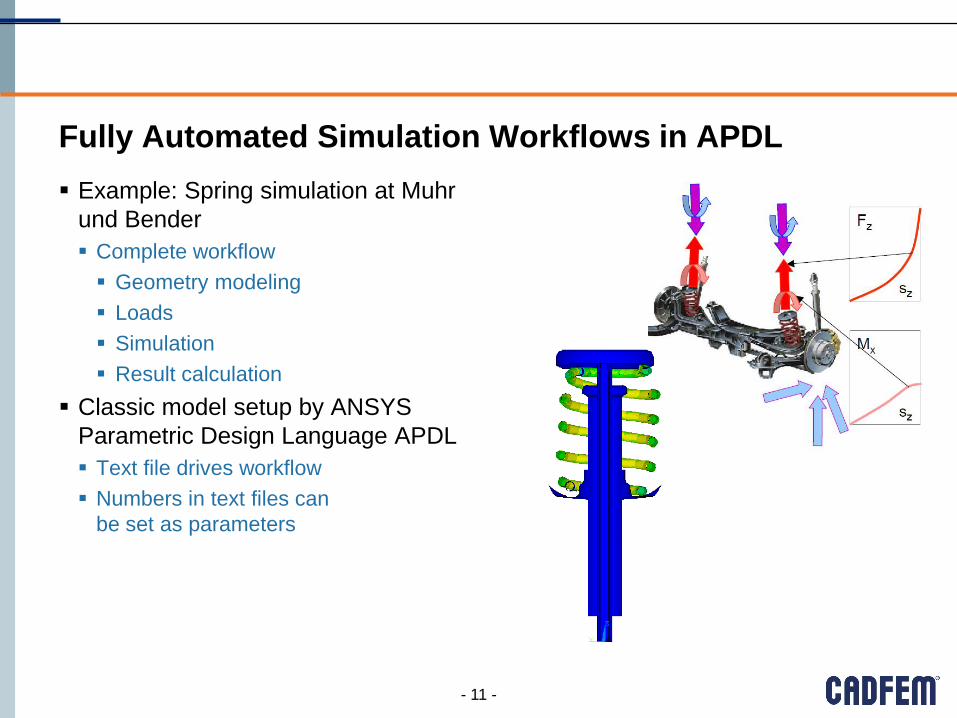
Fully Automated Simulation Workflows in APDL
- 11 -
Example: Spring simulation at Muhr
und Bender
Complete workflow
Geometry modeling
Loads
Simulation
Result calculation
Classic model setup by ANSYS
Parametric Design Language APDL
Text file drives workflow
Numbers in text files can
be set as parameters
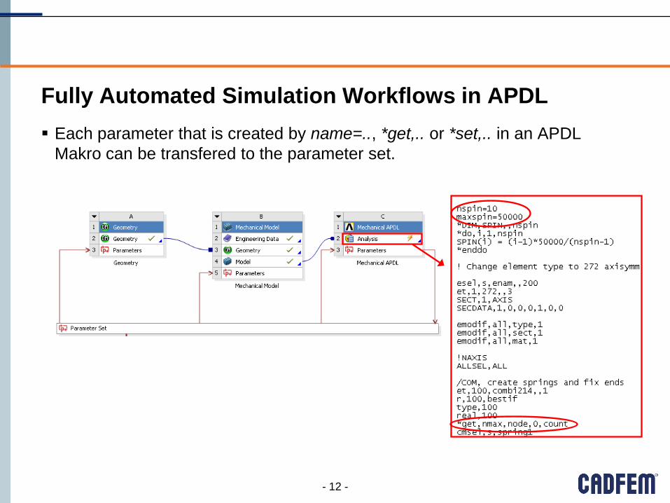
Each parameter that is created by name=.., *get,.. or *set,.. in an APDL
Makro can be transfered to the parameter set.
- 12 -
Fully Automated Simulation Workflows in APDL
Manual Variation
Understand your Design
PRACE Autumn School 2013 - Industry Oriented HPC Simulations, September 21-27,
University of Ljubljana, Faculty of Mechanical Engineering, Ljubljana, Slovenia
Understand your Design
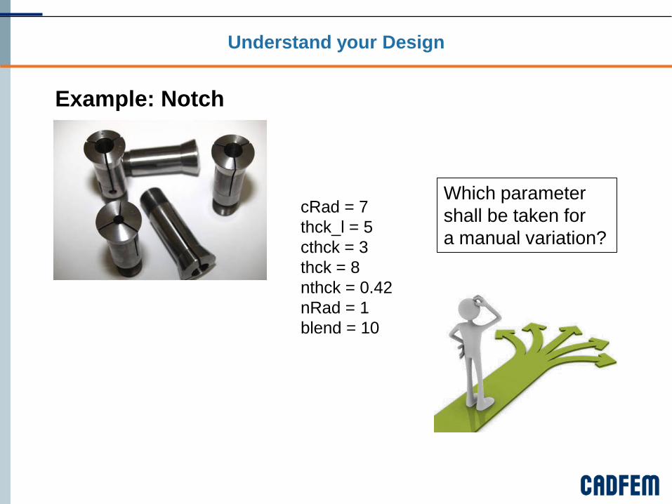
Which parameter
shall be taken for
a manual variation?
Example: Notch
cRad = 7
thck_l = 5
cthck = 3
thck = 8
nthck = 0.42
nRad = 1
blend = 10
Understand your Design
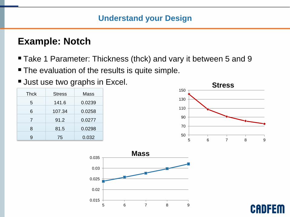
Example: Notch
Take 1 Parameter: Thickness (thck) and vary it between 5 and 9
The evaluation of the results is quite simple.
Just use two graphs in Excel.
Thck Stress Mass
5 141.6 0.0239
6 107.34 0.0258
7 91.2 0.0277
8 81.5 0.0298
9 75 0.032 50
70
90
110
130
150
5 6 7 8 9
Stress
0.015
0.02
0.025
0.03
0.035
5 6 7 8 9
Mass
Understand your Design
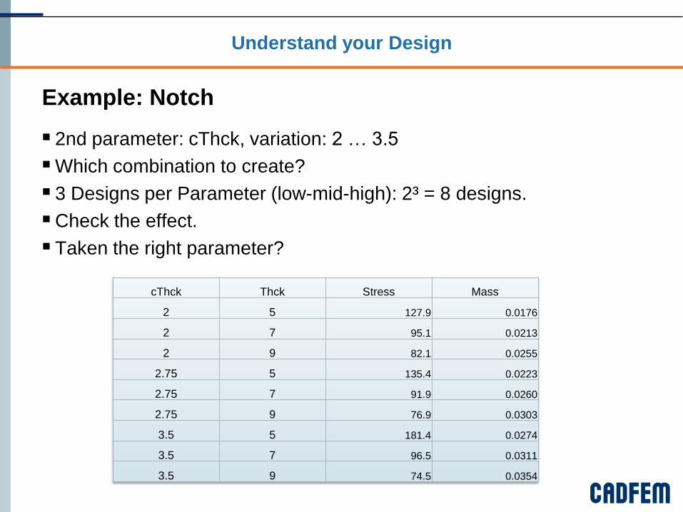
Example: Notch
2nd parameter: cThck, variation: 2 … 3.5
Which combination to create?
3 Designs per Parameter (low-mid-high): 2³ = 8 designs.
Check the effect.
Taken the right parameter?
cThck Thck Stress Mass
2 5 127.9 0.0176
2 7 95.1 0.0213
2 9 82.1 0.0255
2.75 5 135.4 0.0223
2.75 7 91.9 0.0260
2.75 9 76.9 0.0303
3.5 5 181.4 0.0274
3.5 7 96.5 0.0311
3.5 9 74.5 0.0354
Understand your Design
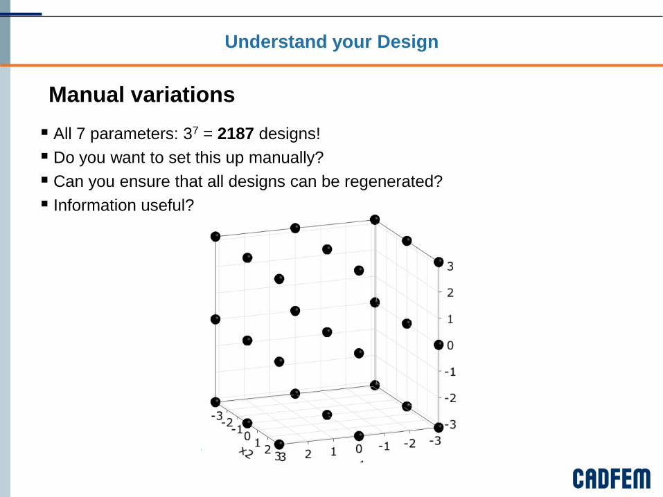
All 7 parameters: 37 = 2187 designs!
Do you want to set this up manually?
Can you ensure that all designs can be regenerated?
Information useful?
Manual variations
Understand your Design
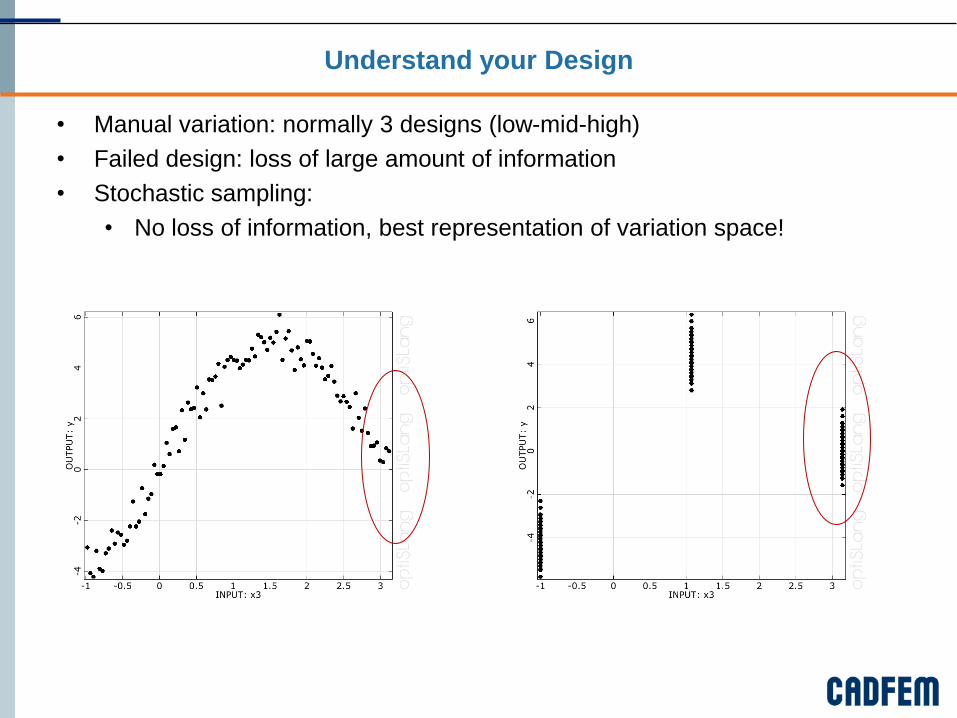
• Manual variation: normally 3 designs (low-mid-high)
• Failed design: loss of large amount of information
• Stochastic sampling:
• No loss of information, best representation of variation space!
Understand your Design
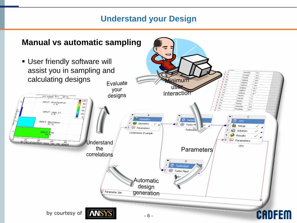
Manual vs automatic sampling
- 6 -
User friendly software will
assist you in sampling and
calculating designs
by courtesy of
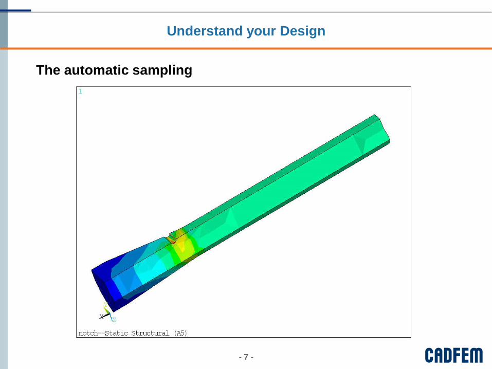
Understand your Design
The automatic sampling
- 7 -
Systematic variation using
optiSLang inside Workbench
Understand your Design
PRACE Autumn School 2013 - Industry Oriented HPC Simulations, September 21-27,
University of Ljubljana, Faculty of Mechanical Engineering, Ljubljana, Slovenia
Understand your Design
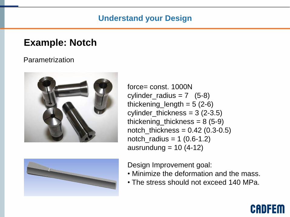
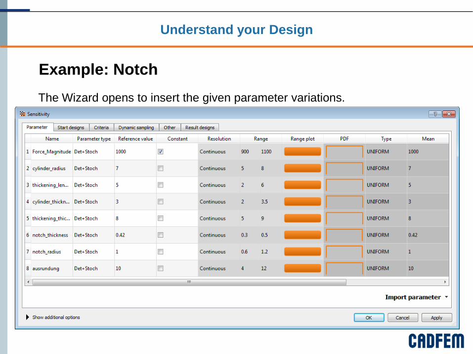
Parametrization
Example: Notch
force= const. 1000N
cylinder_radius = 7 (5-8)
thickening_length = 5 (2-6)
cylinder_thickness = 3 (2-3.5)
thickening_thickness = 8 (5-9)
notch_thickness = 0.42 (0.3-0.5)
notch_radius = 1 (0.6-1.2)
ausrundung = 10 (4-12)
Design Improvement goal:
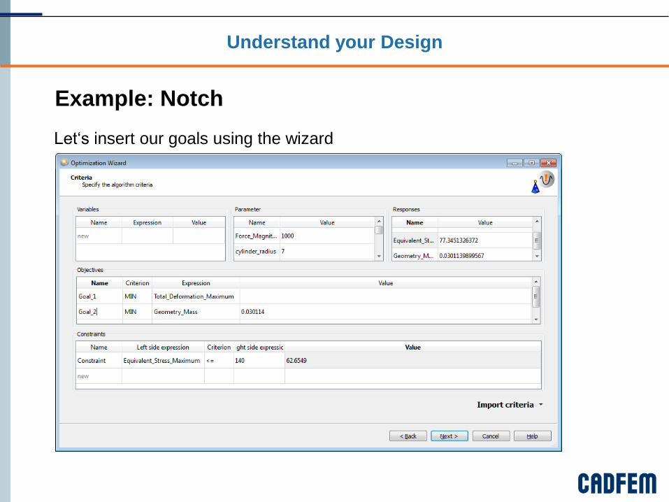
• Minimize the deformation and the mass.
• The stress should not exceed 140 MPa.
Understand your Design
- 2 -
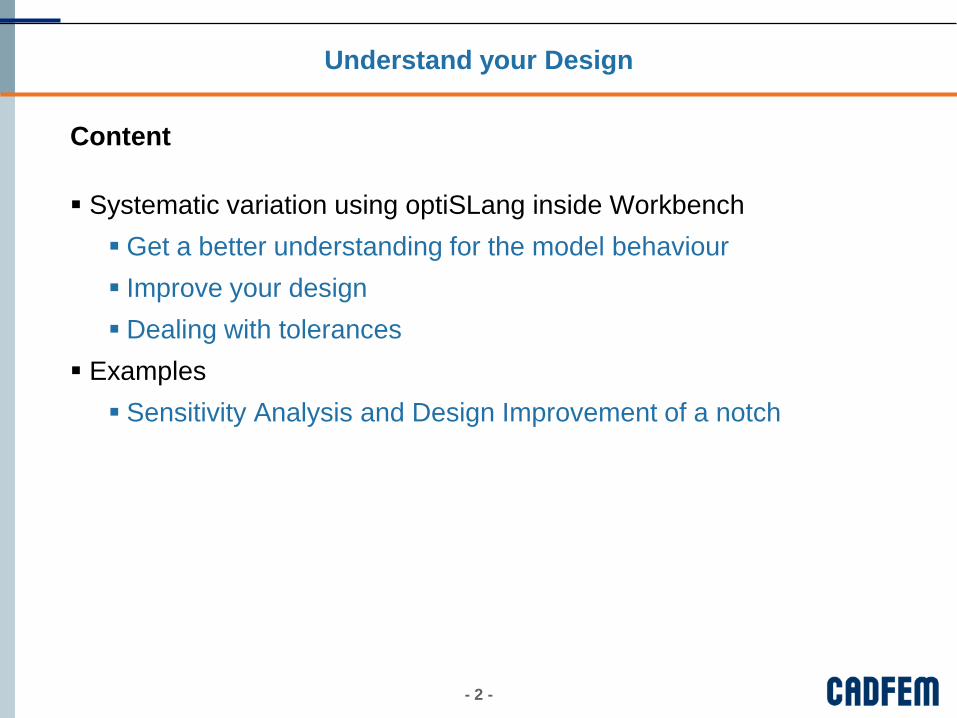
Systematic variation using optiSLang inside Workbench
Get a better understanding for the model behaviour
Improve your design
Dealing with tolerances
Examples
Sensitivity Analysis and Design Improvement of a notch
Content
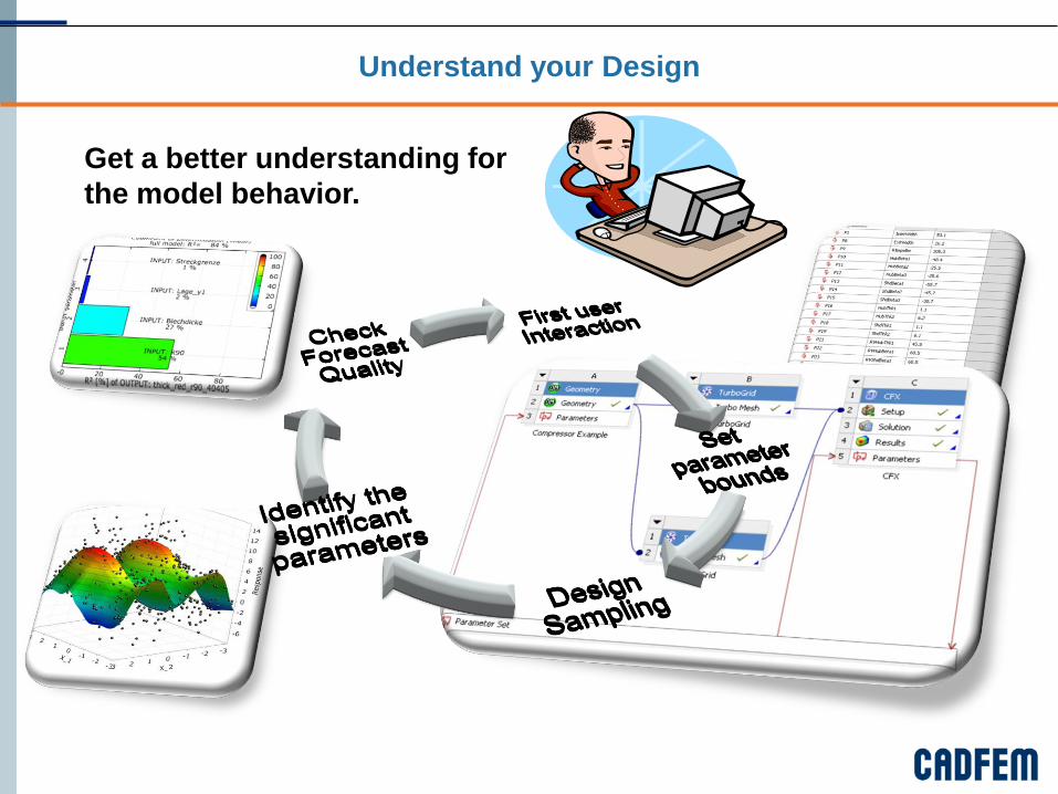
Understand your Design
Get a better understanding for
the model behavior.
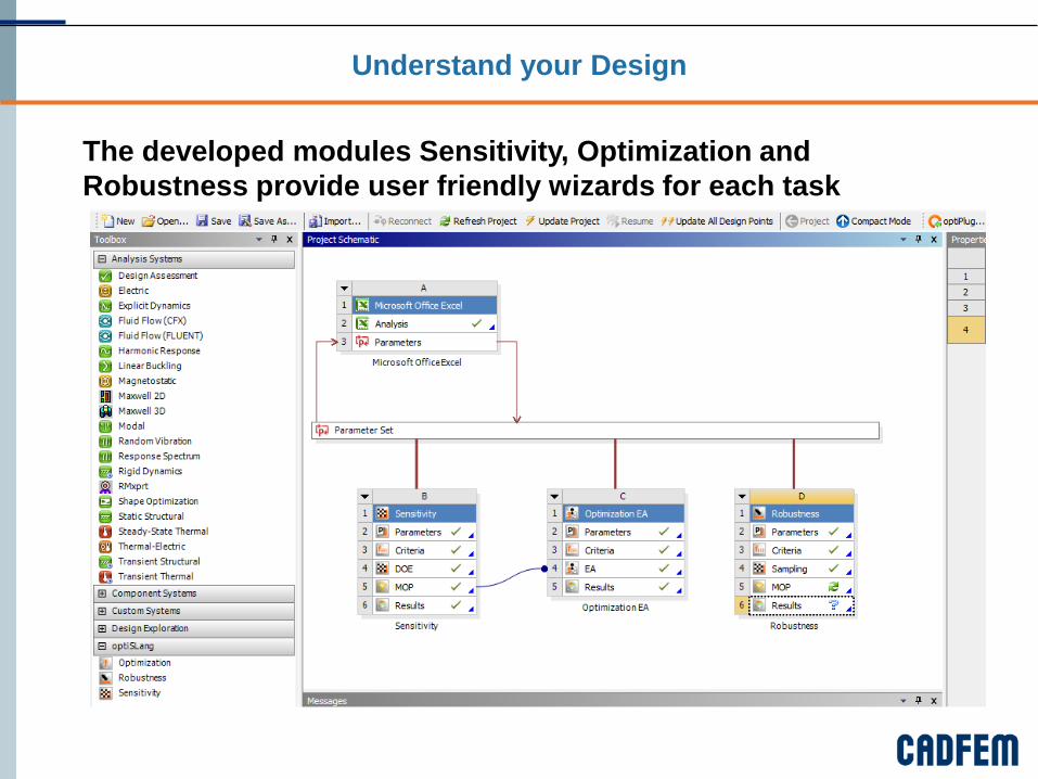
Understand your Design
The developed modules Sensitivity, Optimization and
Robustness provide user friendly wizards for each task
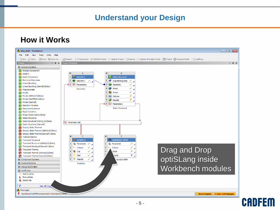
Understand your Design
How it Works
- 5 -
Drag and Drop
optiSLang inside
Workbench modules
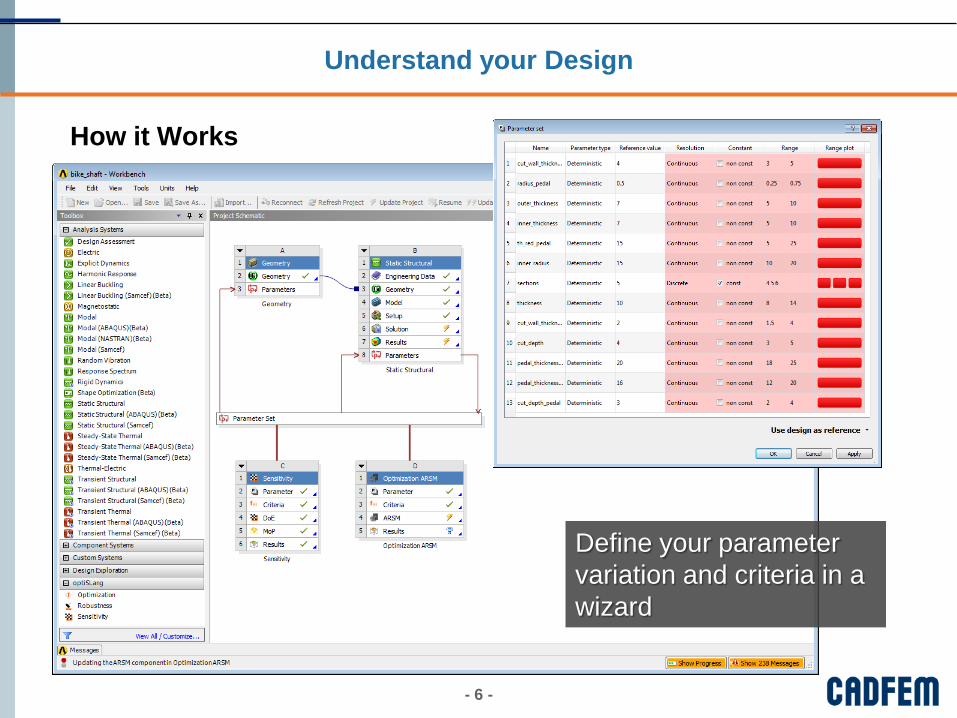
Understand your Design
How it Works
- 6 -
Define your parameter
variation and criteria in a
wizard
Understand your Design
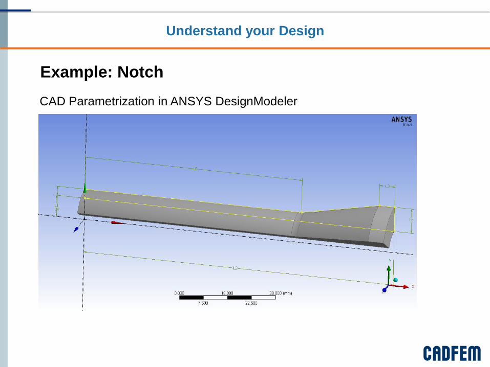
CAD Parametrization in ANSYS DesignModeler
Example: Notch
Understand your Design
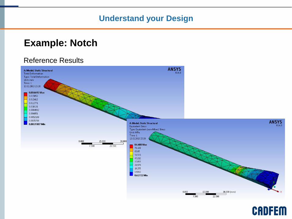
Reference Results
Example: Notch
Understand your Design
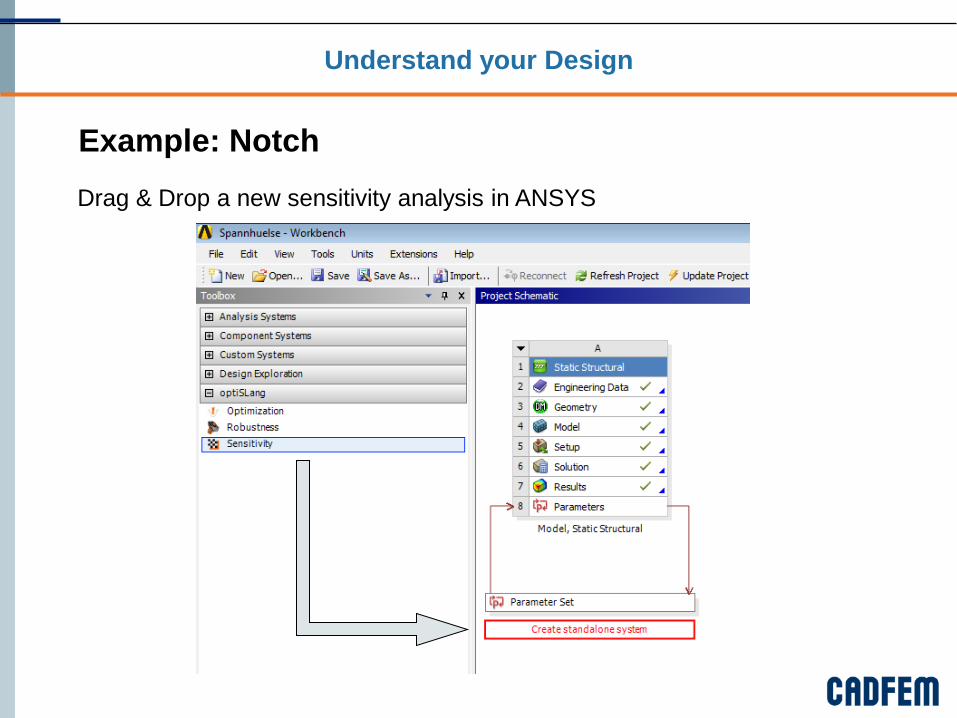
Drag & Drop a new sensitivity analysis in ANSYS
Example: Notch
Understand your Design
The Wizard opens to insert the given parameter variations.
Example: Notch
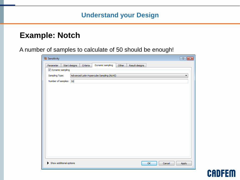
Understand your Design
A number of samples to calculate of 50 should be enough!
Example: Notch
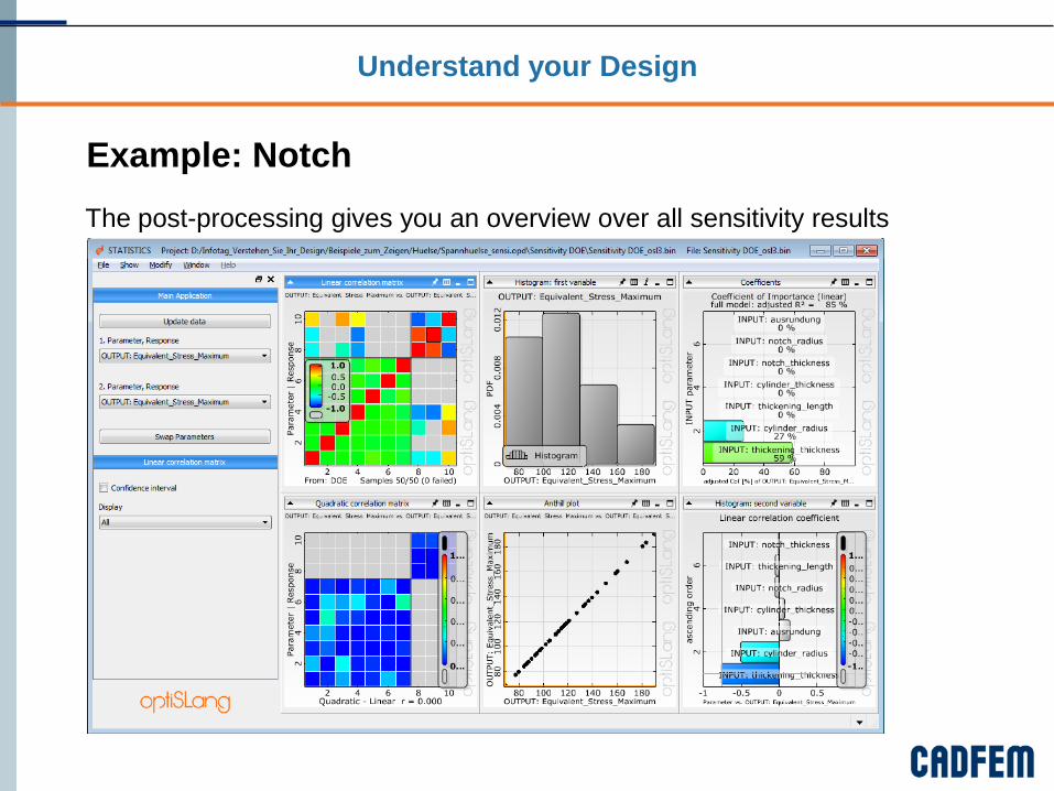
Understand your Design
The post-processing gives you an overview over all sensitivity results
Example: Notch
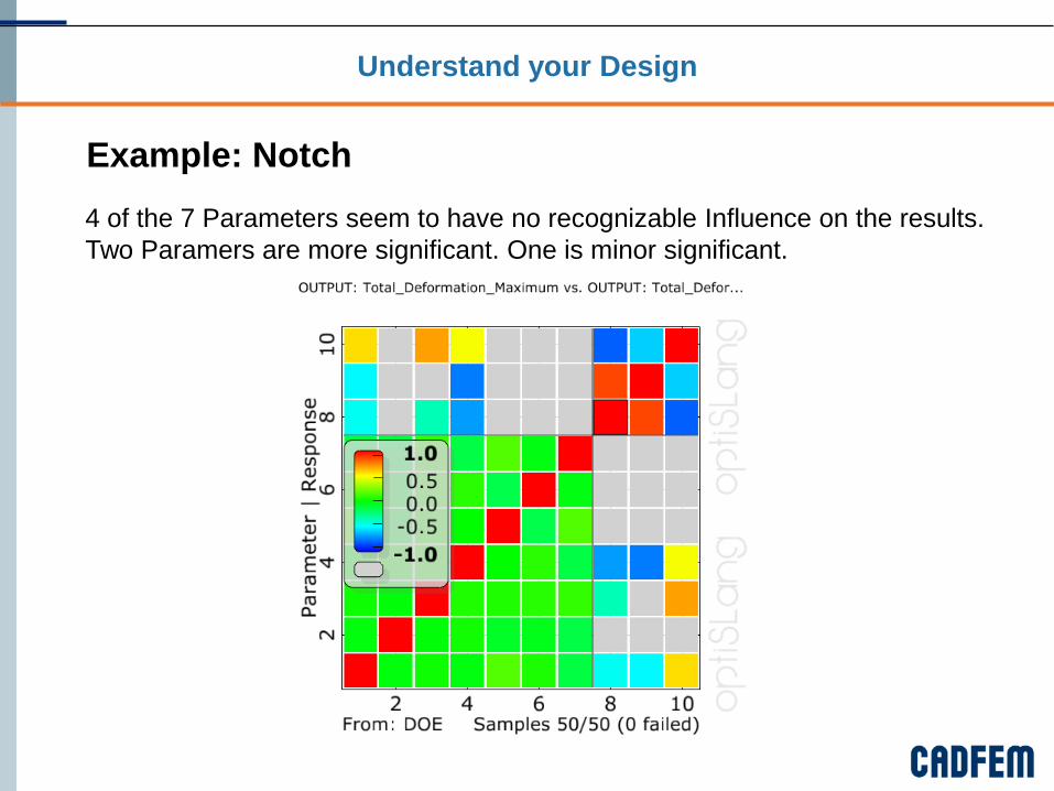
Understand your Design
4 of the 7 Parameters seem to have no recognizable Influence on the results.
Two Paramers are more significant. One is minor significant.
Example: Notch
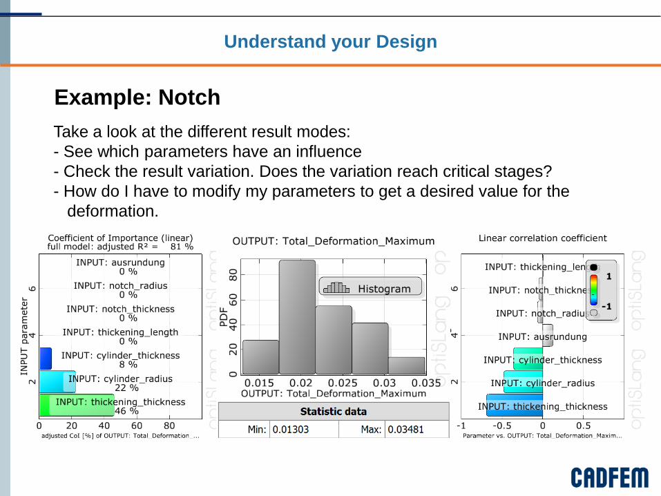
Understand your Design
Take a look at the different result modes:
- See which parameters have an influence
- Check the result variation. Does the variation reach critical stages?
- How do I have to modify my parameters to get a desired value for the
deformation.
Example: Notch
Understand your Design
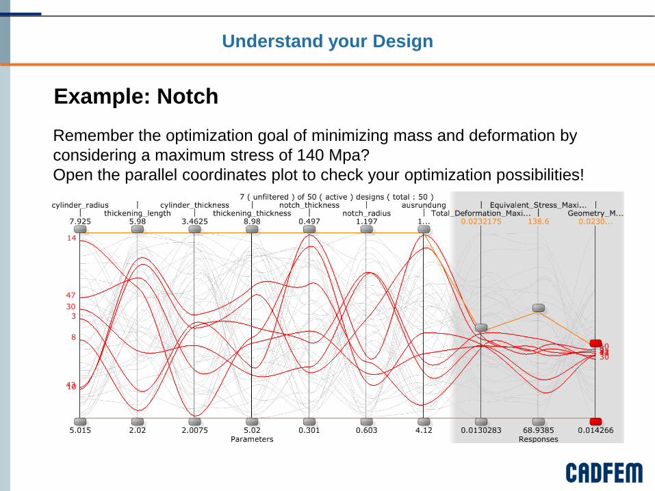
Remember the optimization goal of minimizing mass and deformation by
considering a maximum stress of 140 Mpa?
Open the parallel coordinates plot to check your optimization possibilities!
Example: Notch
Understand your Design
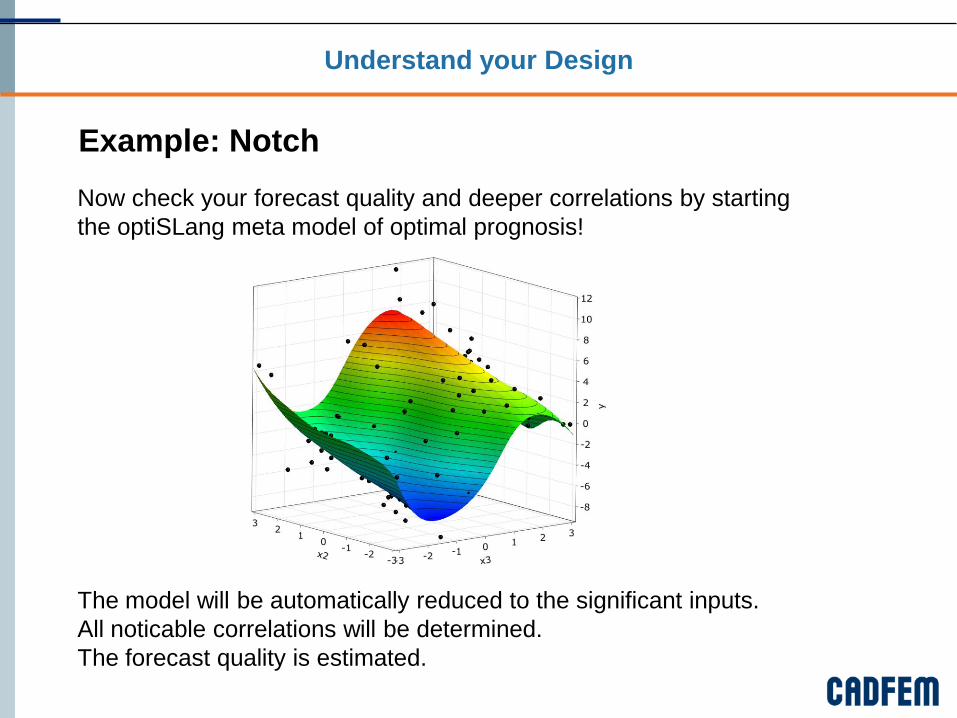
Now check your forecast quality and deeper correlations by starting
the optiSLang meta model of optimal prognosis!
The model will be automatically reduced to the significant inputs.
All noticable correlations will be determined.
The forecast quality is estimated.
Example: Notch
Understand your Design
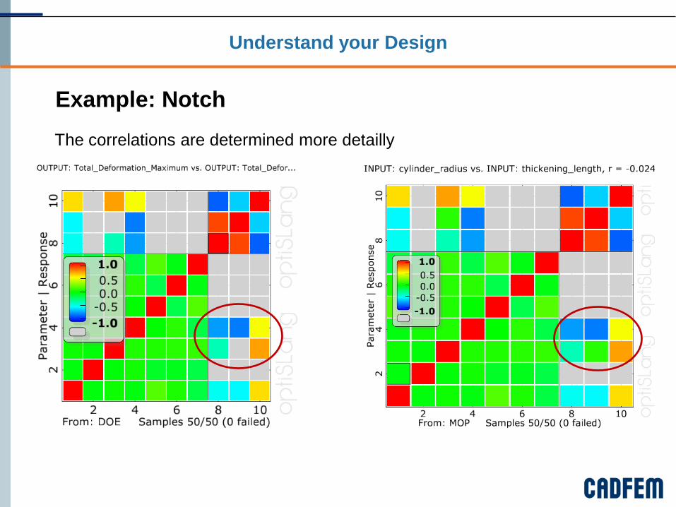
The correlations are determined more detailly
Example: Notch
Understand your Design
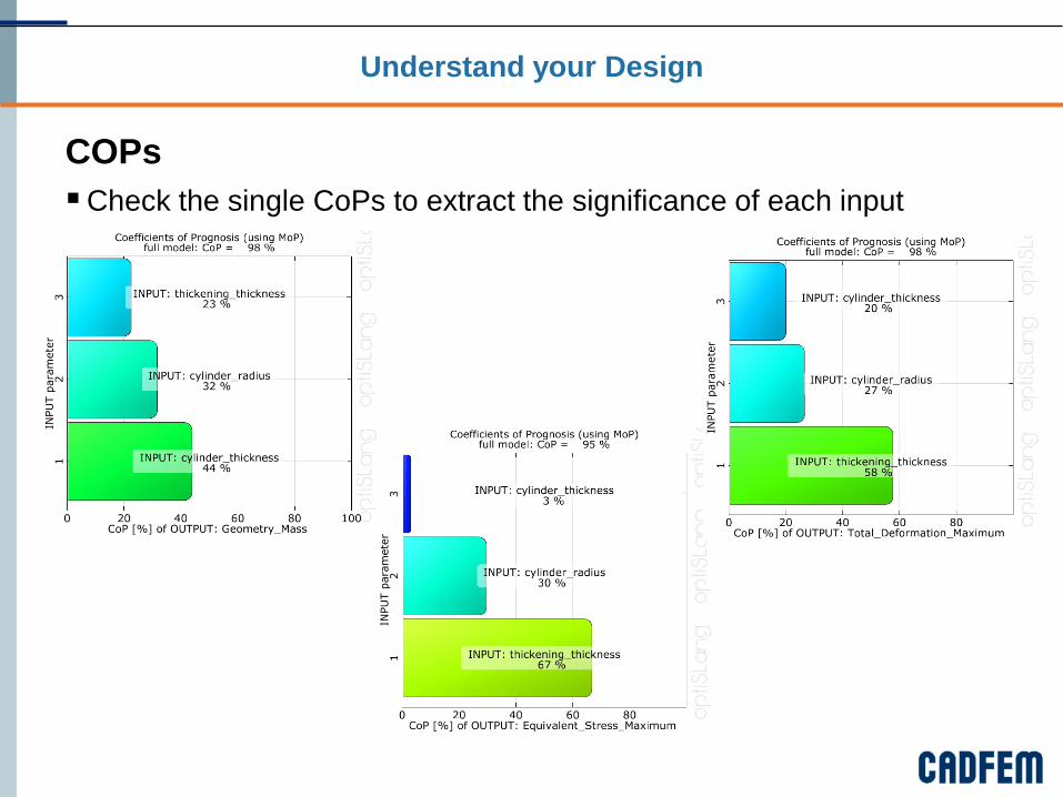
COPs
Check the single CoPs to extract the significance of each input
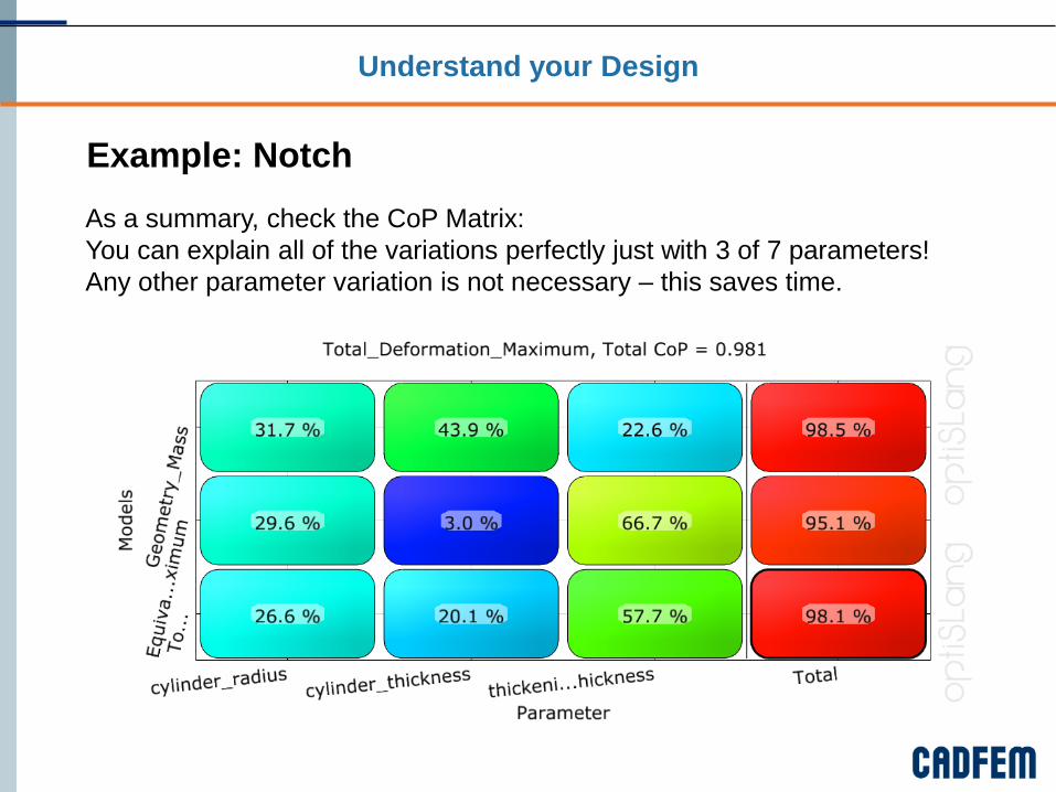
Understand your Design
As a summary, check the CoP Matrix:
You can explain all of the variations perfectly just with 3 of 7 parameters!
Any other parameter variation is not necessary – this saves time.
Example: Notch
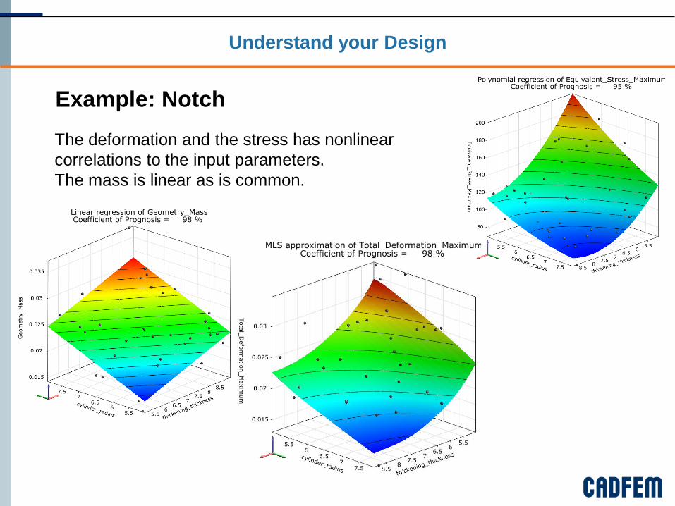
Understand your Design
The deformation and the stress has nonlinear
correlations to the input parameters.
The mass is linear as is common.
Example: Notch
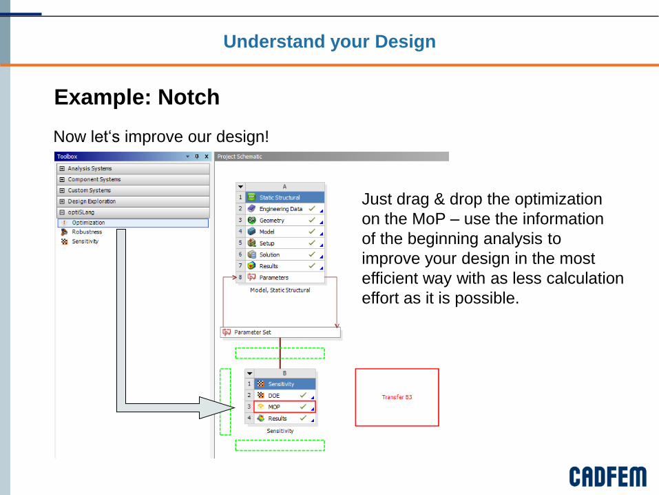
Understand your Design
Now let‘s improve our design!
Example: Notch
Just drag & drop the optimization
on the MoP – use the information
of the beginning analysis to
improve your design in the most
efficient way with as less calculation
effort as it is possible.
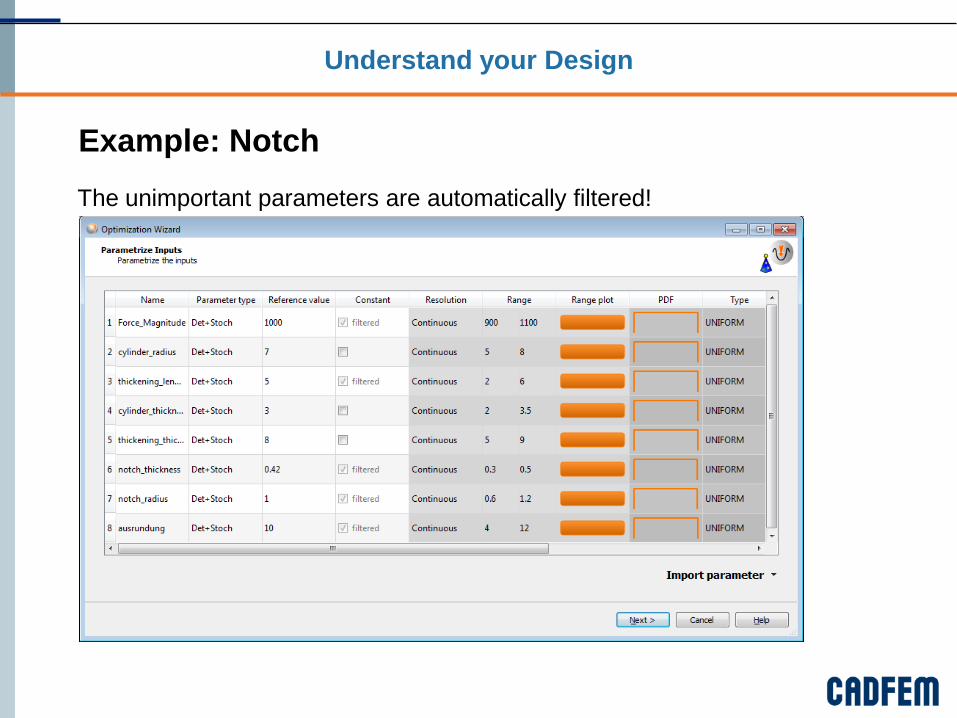
Understand your Design
The unimportant parameters are automatically filtered!
Example: Notch
Understand your Design
Let‘s insert our goals using the wizard
Example: Notch
Understand your Design
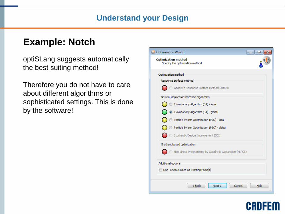
optiSLang suggests automatically
the best suiting method!
Therefore you do not have to care
about different algorithms or
sophisticated settings. This is done
by the software!
Example: Notch
Understand your Design
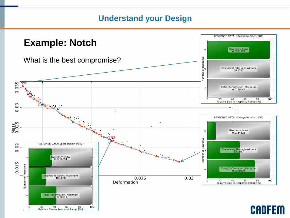
What is the best compromise?
Example: Notch
Understand your Design
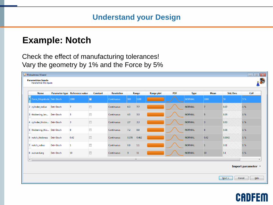
Check the effect of manufacturing tolerances!
Vary the geometry by 1% and the Force by 5%
Example: Notch
Understand your Design
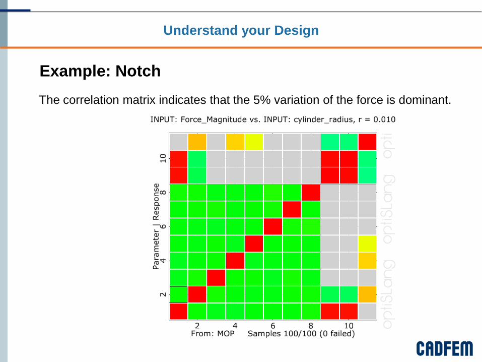
The correlation matrix indicates that the 5% variation of the force is dominant.
Example: Notch
Understand your Design
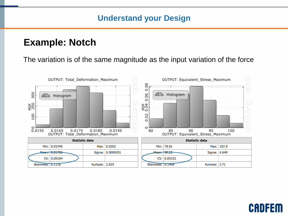
The variation is of the same magnitude as the input variation of the force
Example: Notch
Typical Questions
Understand your Design
PRACE Autumn School 2013 - Industry Oriented HPC Simulations, September 21-27,
University of Ljubljana, Faculty of Mechanical Engineering, Ljubljana, Slovenia
Content
- 1 -
Typical Questions
How to evaluate 1000 designs?
Accuracy and numerical noise
Robust parameter settings
Which settings are the best for my design improvement?
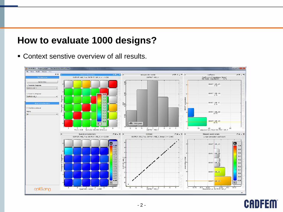
How to evaluate 1000 designs?
Context senstive overview of all results.
- 2 -
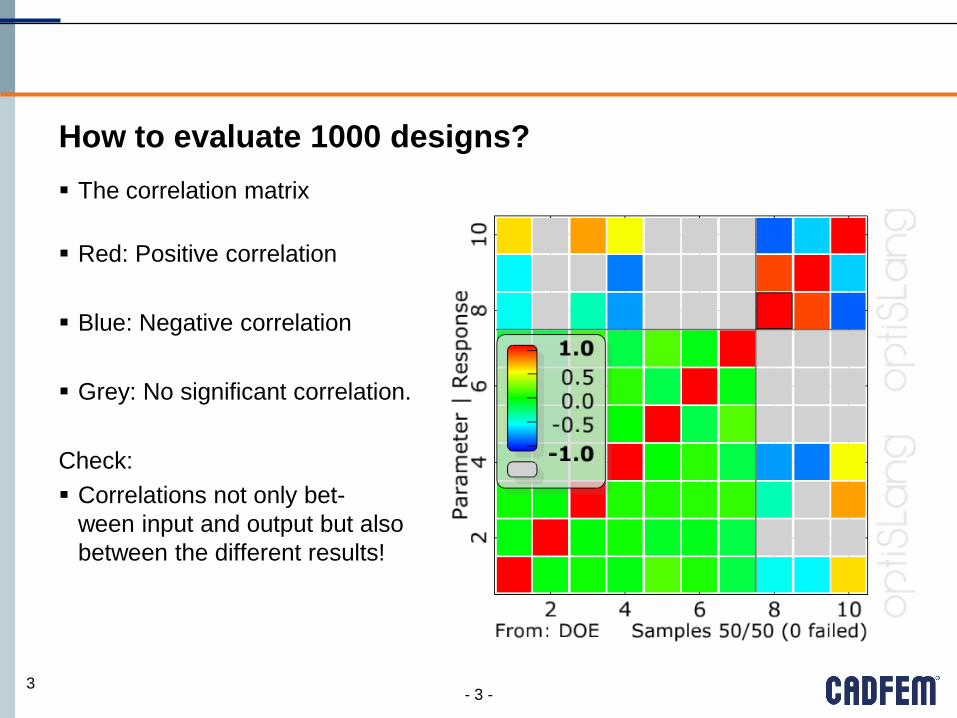
The correlation matrix
Red: Positive correlation
Blue: Negative correlation
Grey: No significant correlation.
Check:
Correlations not only bet-
ween input and output but also
between the different results!
3
How to evaluate 1000 designs?
- 3 -
4
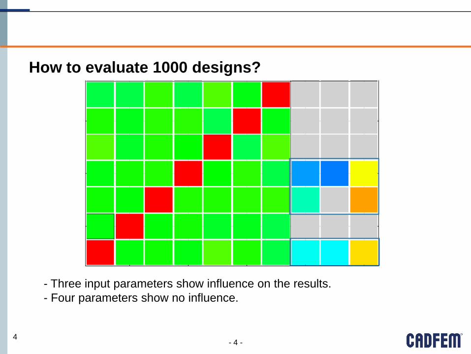
- Three input parameters show influence on the results.
- Four parameters show no influence.
How to evaluate 1000 designs?
- 4 -
5
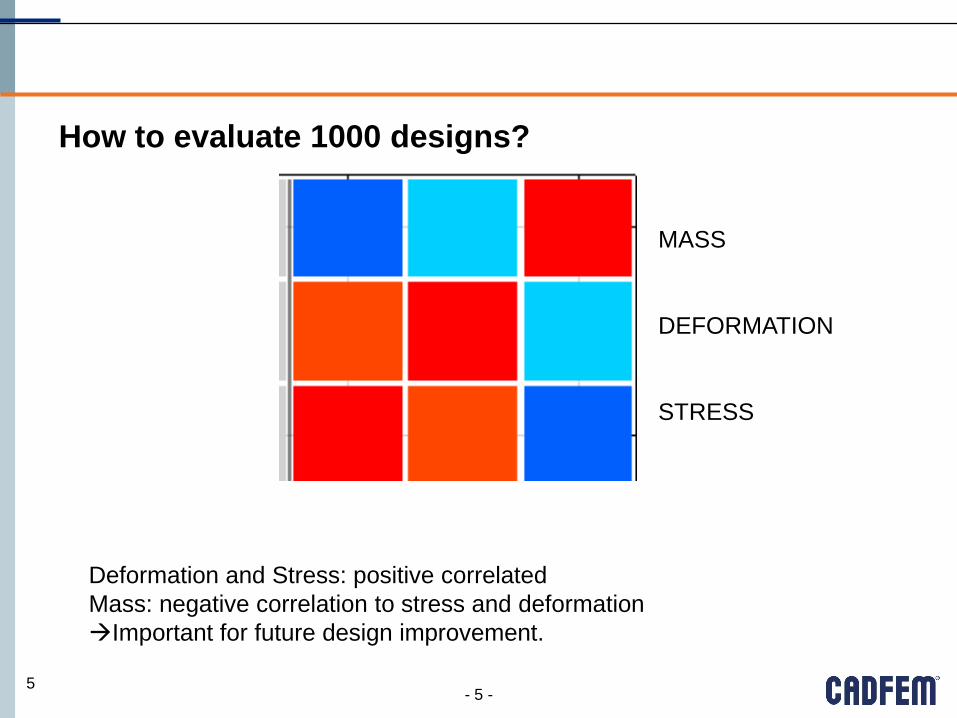
MASS
DEFORMATION
STRESS
Deformation and Stress: positive correlated
Mass: negative correlation to stress and deformation
Important for future design improvement.
How to evaluate 1000 designs?
- 5 -
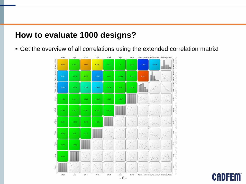
Get the overview of all correlations using the extended correlation matrix!
How to evaluate 1000 designs?
- 6 -
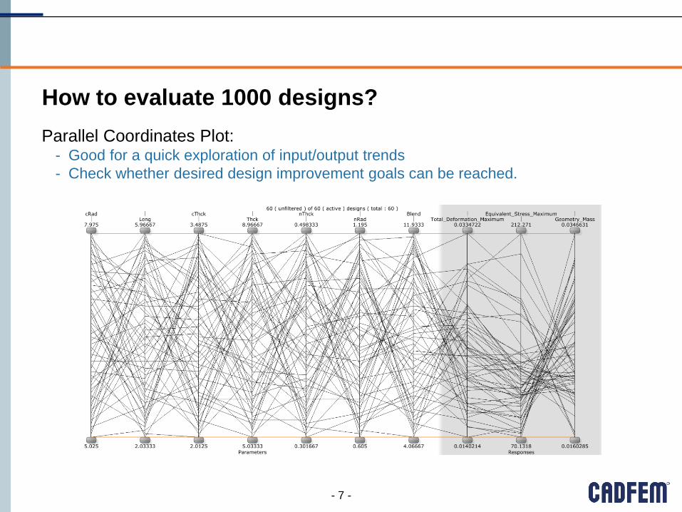
Parallel Coordinates Plot: - Good for a quick exploration of input/output trends
- Check whether desired design improvement goals can be reached.
How to evaluate 1000 designs?
- 7 -
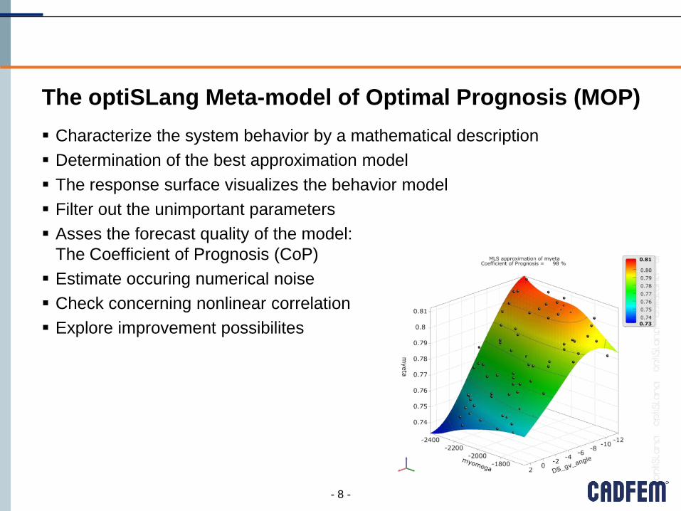
The optiSLang Meta-model of Optimal Prognosis (MOP)
Characterize the system behavior by a mathematical description
Determination of the best approximation model
The response surface visualizes the behavior model
Filter out the unimportant parameters
Asses the forecast quality of the model:
The Coefficient of Prognosis (CoP)
Estimate occuring numerical noise
Check concerning nonlinear correlation
Explore improvement possibilites
- 8 -
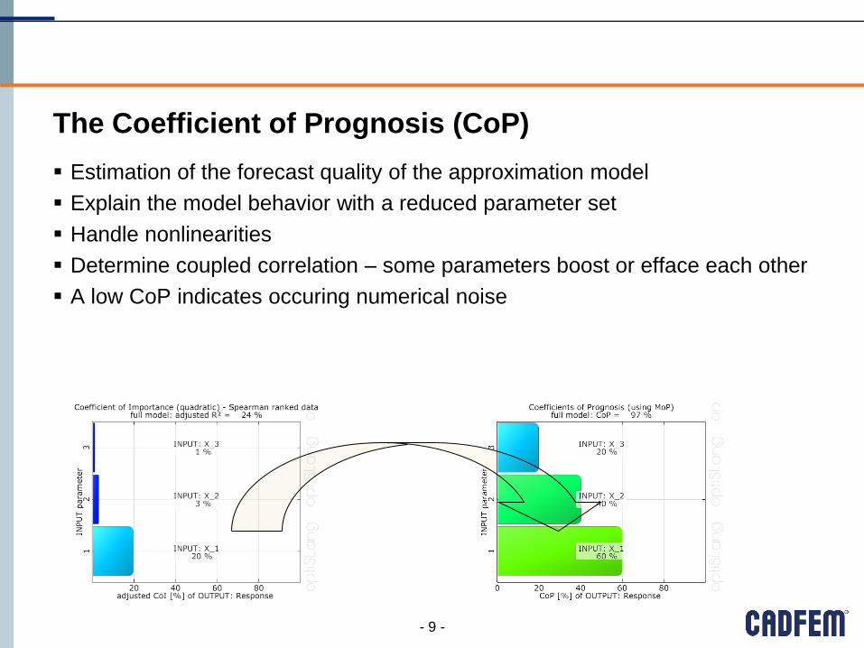
The Coefficient of Prognosis (CoP)
Estimation of the forecast quality of the approximation model
Explain the model behavior with a reduced parameter set
Handle nonlinearities
Determine coupled correlation – some parameters boost or efface each other
A low CoP indicates occuring numerical noise
- 9 -
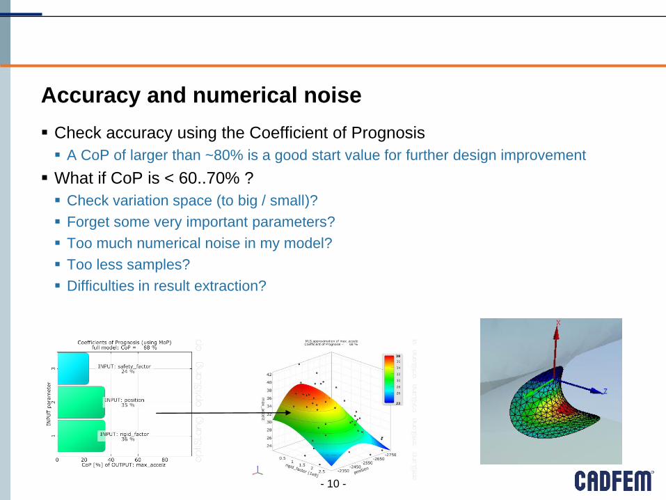
Accuracy and numerical noise
Check accuracy using the Coefficient of Prognosis
A CoP of larger than ~80% is a good start value for further design improvement
What if CoP is < 60..70% ?
Check variation space (to big / small)?
Forget some very important parameters?
Too much numerical noise in my model?
Too less samples?
Difficulties in result extraction?
- 10 -
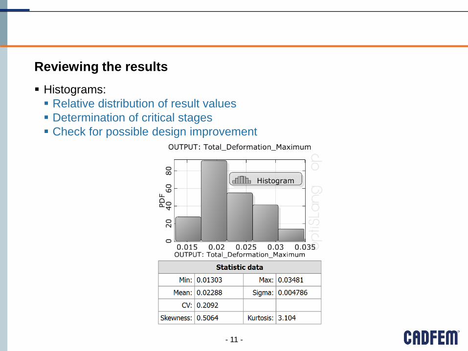
Reviewing the results
- 11 -
Histograms:
Relative distribution of result values
Determination of critical stages
Check for possible design improvement
Robust parameter settings
- 12 -
What are robust parameter setting?
The solution always converges
The geometry can always be generated
The mesh can always be created
Can we determine robust parameter settings in advance?
Do we even need them?
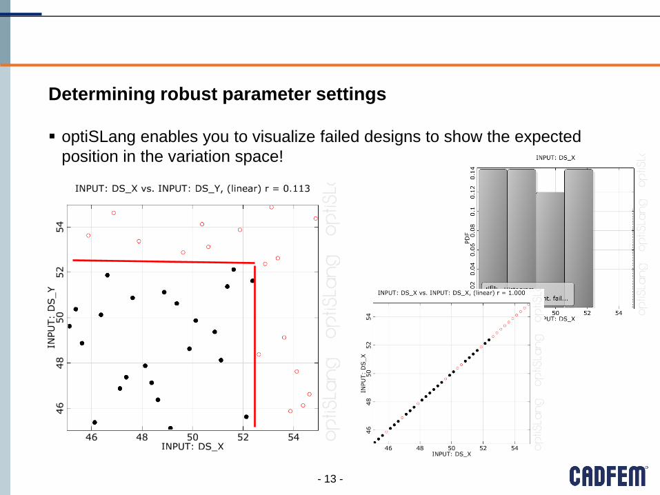
Determining robust parameter settings
- 13 -
optiSLang enables you to visualize failed designs to show the expected
position in the variation space!
BUT - Do we need always converging and regeneratable models?
- 14 -
optiSLang can deal with failed designs!
Do not limit your variation space!
Rather accept failed designs than loosing information!
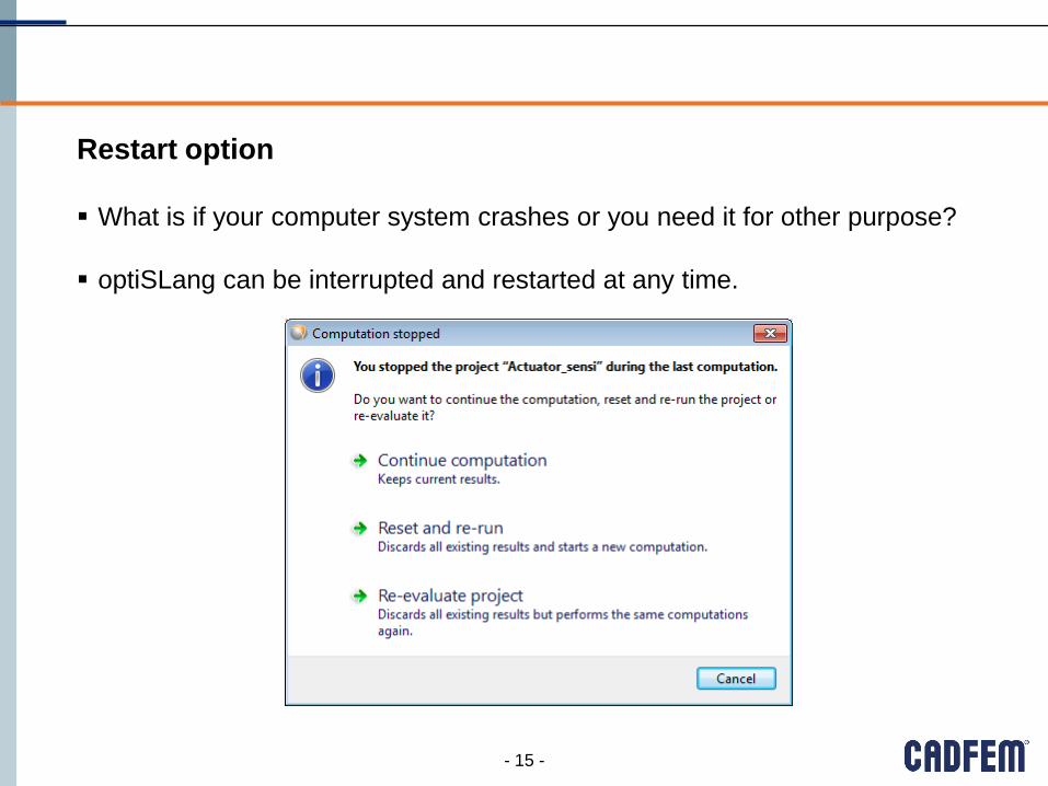
Restart option
- 15 -
What is if your computer system crashes or you need it for other purpose?
optiSLang can be interrupted and restarted at any time.
Understand your Design
Hard- and Software for Performant Design Variation
- 0 -
PRACE Autumn School 2013 - Industry Oriented HPC Simulations, September 21-27,
University of Ljubljana, Faculty of Mechanical Engineering, Ljubljana, Slovenia
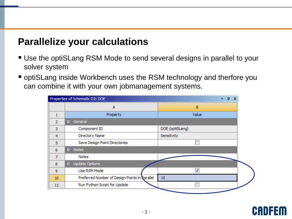
Parallelize your calculations
- 1 -
Use the optiSLang RSM Mode to send several designs in parallel to your
solver system
optiSLang inside Workbench uses the RSM technology and therfore you
can combine it with your own jobmanagement systems.
Hardware
- 2 -
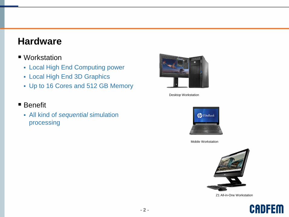
Workstation
Local High End Computing power
Local High End 3D Graphics
Up to 16 Cores and 512 GB Memory
Benefit
All kind of sequential simulation
processing
Desktop Workstation
Z1 All-in-One Workstation
Mobile Workstation
Hardware
- 3 -
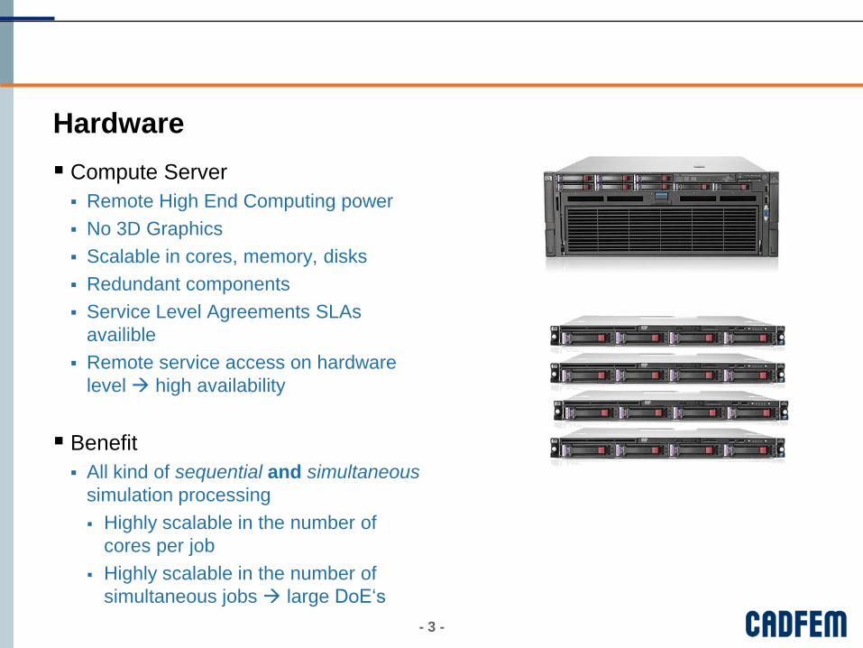
Compute Server
Remote High End Computing power
No 3D Graphics
Scalable in cores, memory, disks
Redundant components
Service Level Agreements SLAs
availible
Remote service access on hardware
level high availability
Benefit
All kind of sequential and simultaneous
simulation processing
Highly scalable in the number of
cores per job
Highly scalable in the number of
simultaneous jobs large DoE‘s
Hardware
- 4 -
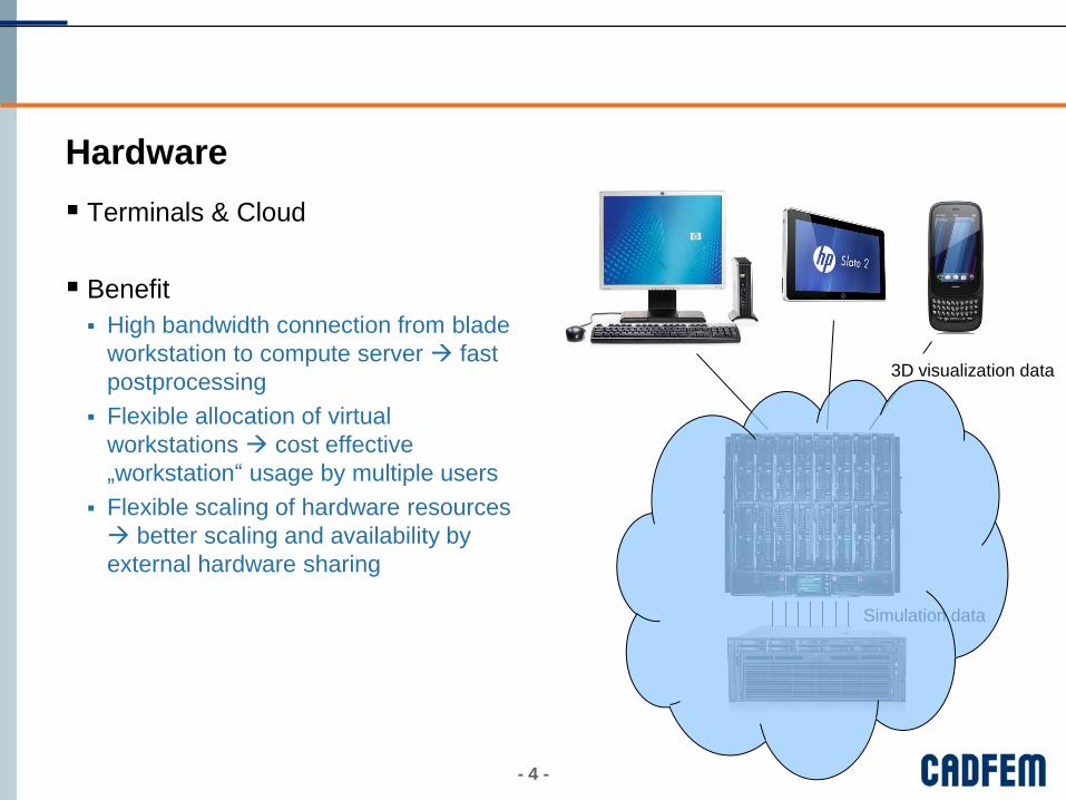
Terminals & Cloud
Benefit
High bandwidth connection from blade
workstation to compute server fast
postprocessing
Flexible allocation of virtual
workstations cost effective
„workstation“ usage by multiple users
Flexible scaling of hardware resources
better scaling and availability by
external hardware sharing
Simulation data
3D visualization data
- 5 -
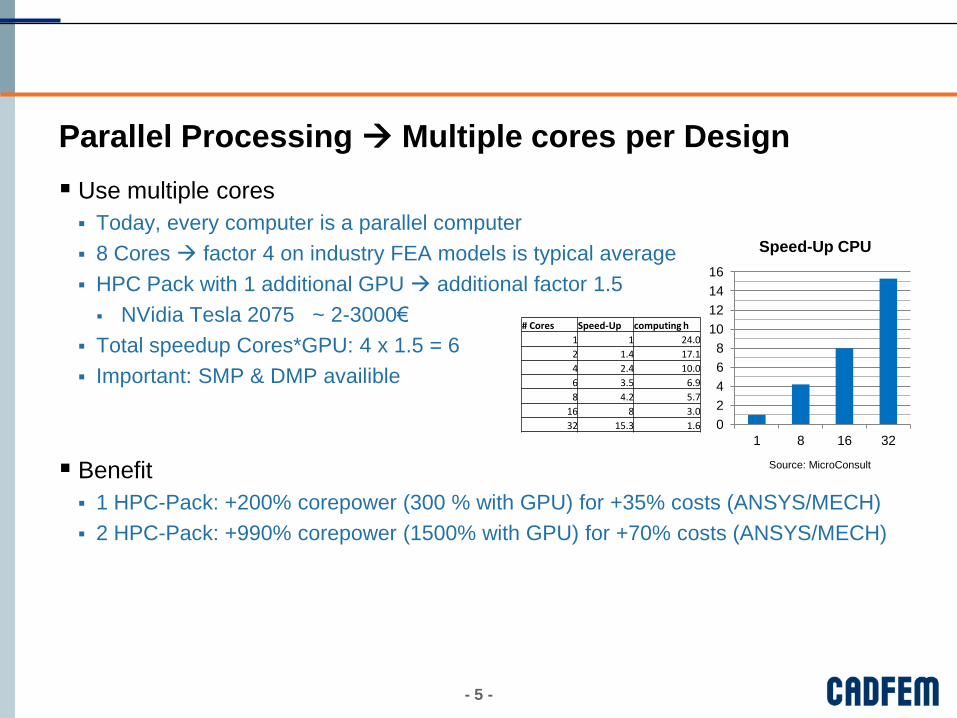
Parallel Processing Multiple cores per Design
Use multiple cores
Today, every computer is a parallel computer
8 Cores factor 4 on industry FEA models is typical average
HPC Pack with 1 additional GPU additional factor 1.5
NVidia Tesla 2075 ~ 2-3000€
Total speedup Cores*GPU: 4 x 1.5 = 6
Important: SMP & DMP availible
Benefit
1 HPC-Pack: +200% corepower (300 % with GPU) for +35% costs (ANSYS/MECH)
2 HPC-Pack: +990% corepower (1500% with GPU) for +70% costs (ANSYS/MECH)
# Cores Speed-Up computing h
1 1 24.0
2 1.4 17.1
4 2.4 10.0
6 3.5 6.9
8 4.2 5.7
16 8 3.0
32 15.3 1.6
Source: MicroConsult
0
2
4
6
8
10
12
14
16
1 8 16 32
Speed-Up CPU
- 6 -
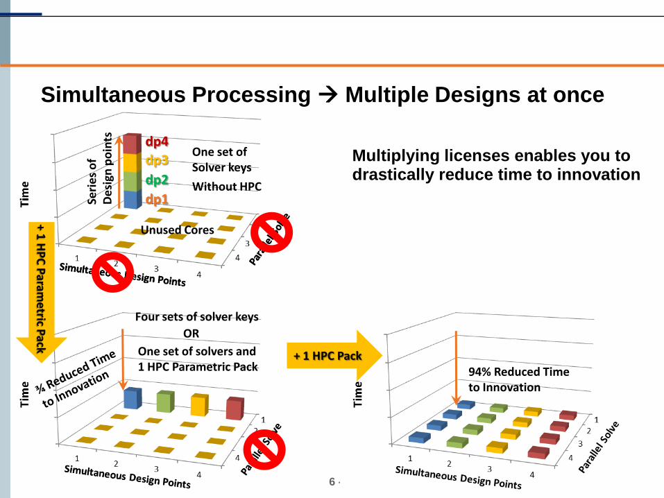
Simultaneous Processing Multiple Designs at once
dp1
dp2
dp3
dp4
Seri
es
of
De
sign
po
ints
Unused Cores
One set of solvers and 1 HPC Parametric Pack
Without HPC
94% Reduced Time to Innovation
Multiplying licenses enables you to drastically reduce time to innovation
One set of Solver keys
Four sets of solver keys
OR
+ 1 HPC Pack
+ 1 H
PC
Param
etric Pack
- 7 -
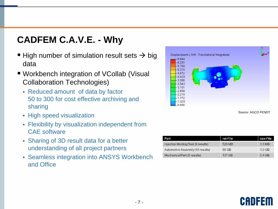
High number of simulation result sets big
data
Workbench integration of VCollab (Visual
Collaboration Technologies)
Reduced amount of data by factor
50 to 300 for cost effective archiving and
sharing
High speed visualization
Flexibility by visualization independent from
CAE software
Sharing of 3D result data for a better
understanding of all project partners
Seamless integration into ANSYS Workbench
and Office
CADFEM C.A.V.E. - Why
Source: AGCO FENDT
CADFEM C.A.V.E. - Summary
High data compression rate
Minimized costs for archiving
High speed visualization
Improves communication and
understanding by sharing results
3D Result viewing for everyone free of
charge
Seamless Workbench integration
Safety First: Automated consistency
Time effective result extraction
Understand your design
Optimization
PRACE Autumn School 2013 - Industry Oriented HPC Simulations, September 21-27,
University of Ljubljana, Faculty of Mechanical Engineering, Ljubljana, Slovenia
Optimization
- 2 -
Table of contents
1. General Information
2. Optimization Algorithms
Optimization
- 3 -
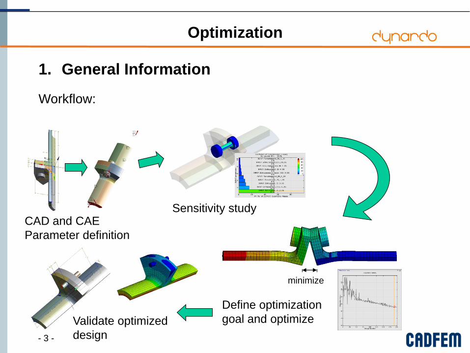
1. General Information
xxx
CAD and CAE
Parameter definition
Sensitivity study
minimize
Define optimization
goal and optimize Validate optimized
design
Workflow:
Optimization
- 4 -
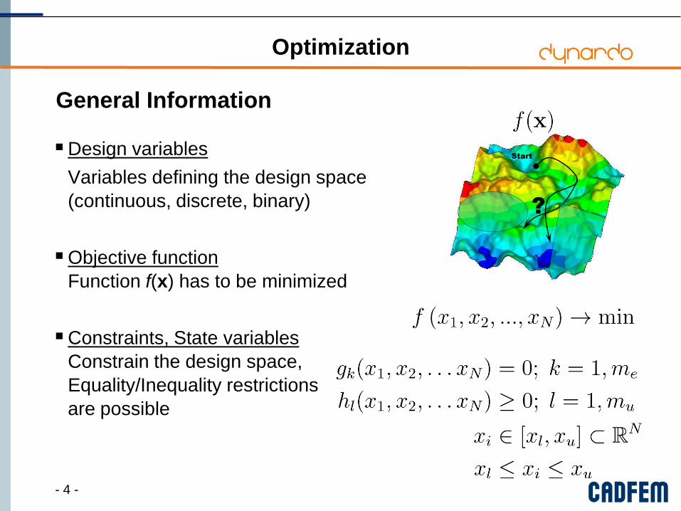
General Information
?
Start Design variables
Variables defining the design space
(continuous, discrete, binary)
Objective function
Function f(x) has to be minimized
Constraints, State variables
Constrain the design space,
Equality/Inequality restrictions
are possible
Optimization
- 5 -
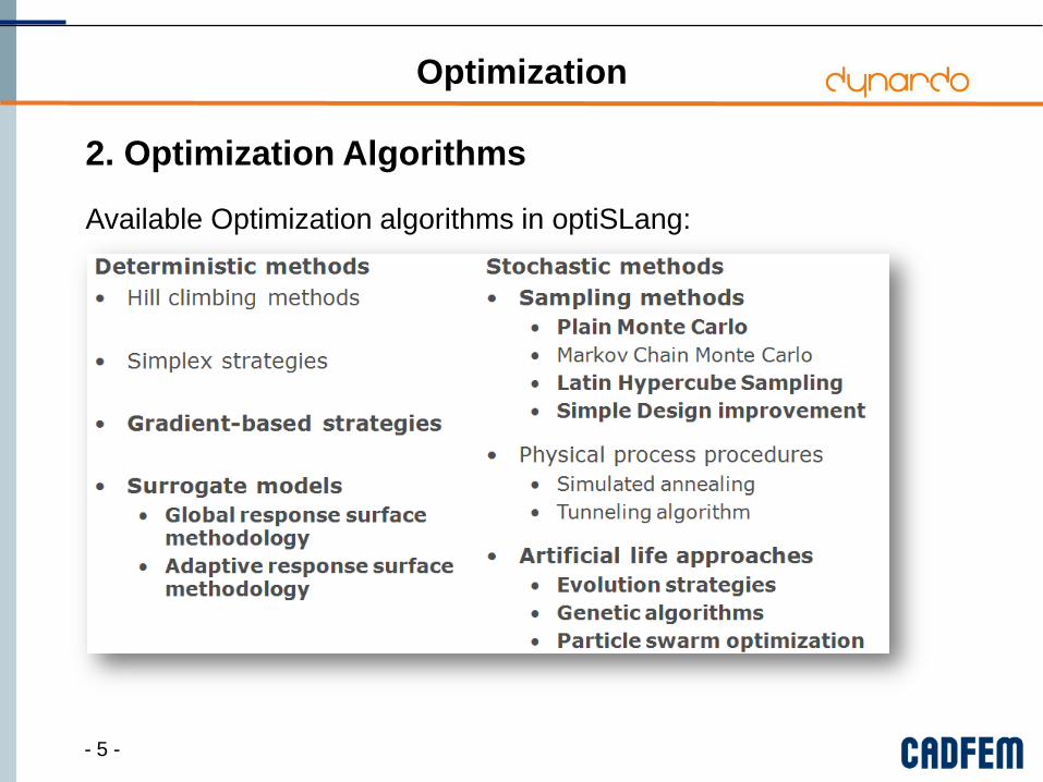
2. Optimization Algorithms
Available Optimization algorithms in optiSLang:
Optimization
- 6 -
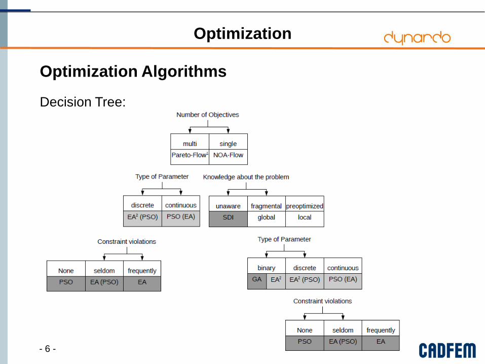
Optimization Algorithms
Decision Tree:
Optimization
- 7 -
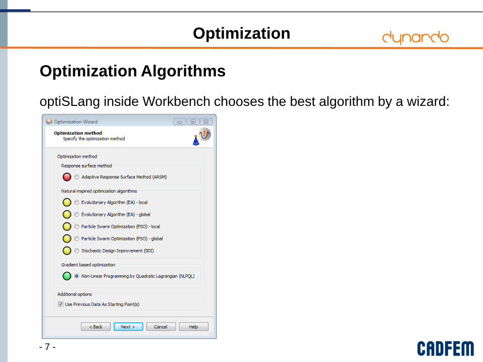
Optimization Algorithms
optiSLang inside Workbench chooses the best algorithm by a wizard:
Optimization
- 8 -
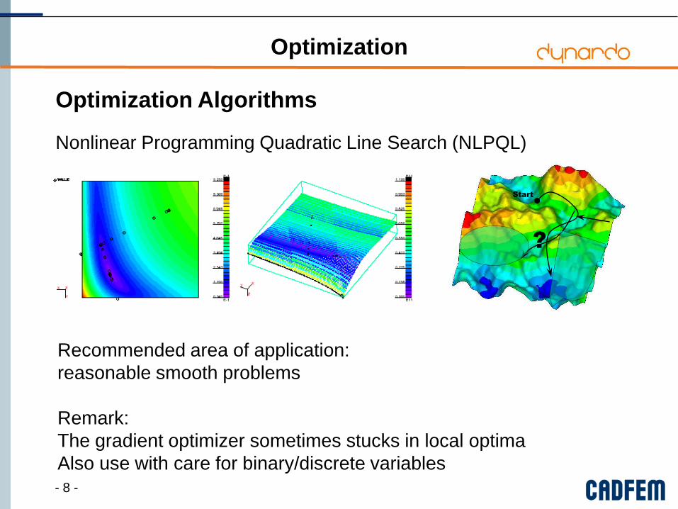
Optimization Algorithms
Nonlinear Programming Quadratic Line Search (NLPQL)
?
Start
Recommended area of application:
reasonable smooth problems
Remark:
The gradient optimizer sometimes stucks in local optima
Also use with care for binary/discrete variables
Optimization
- 9 -
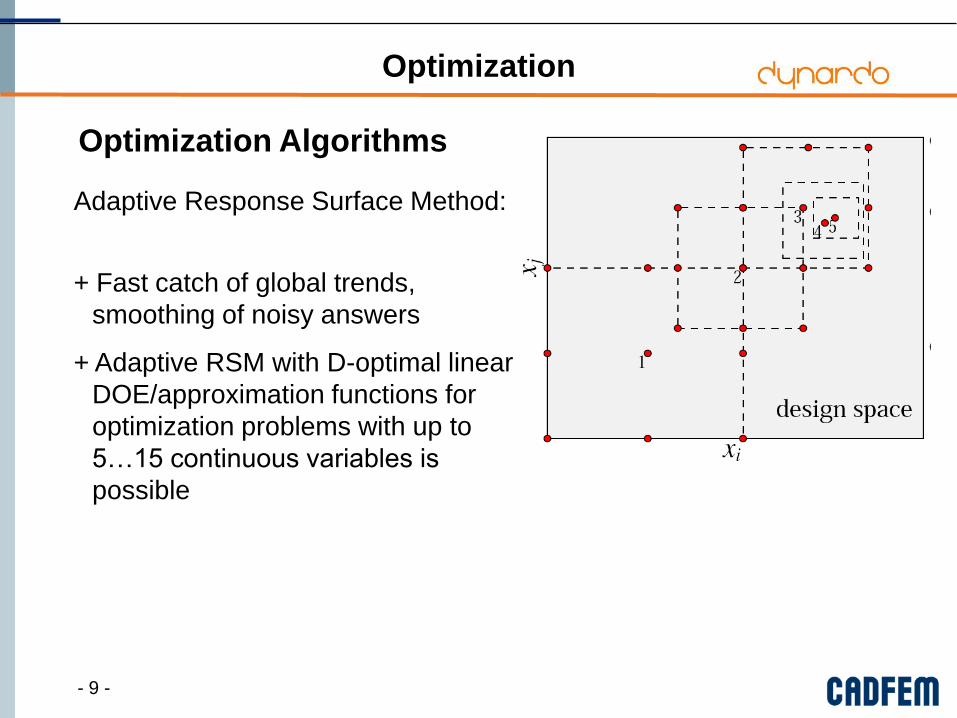
Optimization Algorithms
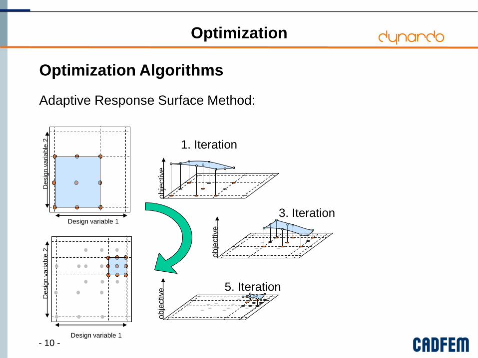
Adaptive Response Surface Method:
+ Fast catch of global trends,
smoothing of noisy answers
+ Adaptive RSM with D-optimal linear
DOE/approximation functions for
optimization problems with up to
5…15 continuous variables is
possible
Optimization
- 10 -
Optimization Algorithms
Adaptive Response Surface Method:
ob
jective
Design variable 1
Desig
n v
ariable
2
ob
jective
ob
jective
Design variable 1
Desig
n v
ariable
2
1. Iteration
3. Iteration
5. Iteration
Optimization
- 11 -
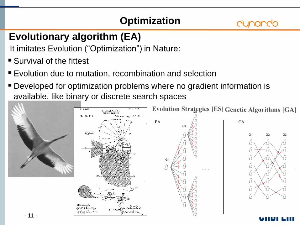
It imitates Evolution (“Optimization”) in Nature:
Survival of the fittest
Evolution due to mutation, recombination and selection
Developed for optimization problems where no gradient information is
available, like binary or discrete search spaces
Genetic Algorithms [GA] Evolution Strategies [ES]
Evolutionary algorithm (EA)
Optimization
- 12 -
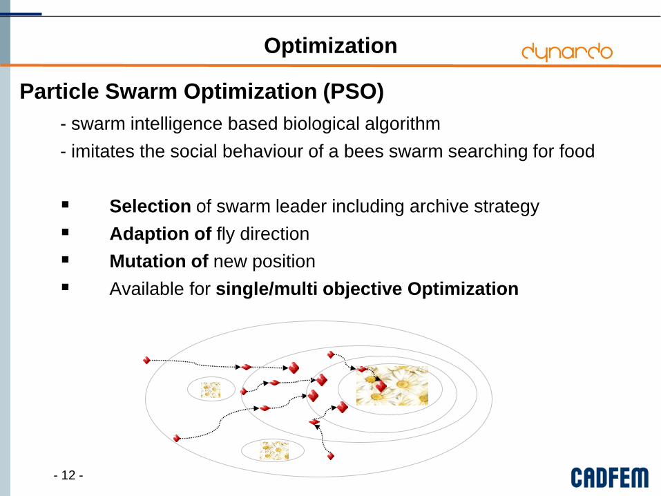
Particle Swarm Optimization (PSO)
- swarm intelligence based biological algorithm
- imitates the social behaviour of a bees swarm searching for food
Selection of swarm leader including archive strategy
Adaption of fly direction
Mutation of new position
Available for single/multi objective Optimization

Optimization
- 13 -
Simple Design Improvement
Improves a proposed design without extensive knowledge about
interactions in design space
Start population by uniform LHS around given start design
The best design is selected as center for the next sampling
The sampling ranges decrease with every generation
Optimization
- 14 -
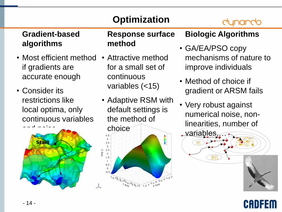
Gradient-based
algorithms
• Most efficient method
if gradients are
accurate enough
• Consider its
restrictions like
local optima, only
continuous variables
and noise
Response surface
method
• Attractive method
for a small set of
continuous
variables (<15)
• Adaptive RSM with
default settings is
the method of
choice
Biologic Algorithms
• GA/EA/PSO copy
mechanisms of nature to
improve individuals
• Method of choice if
gradient or ARSM fails
• Very robust against
numerical noise, non-
linearities, number of
variables,… Start
Optimization
- 15 -
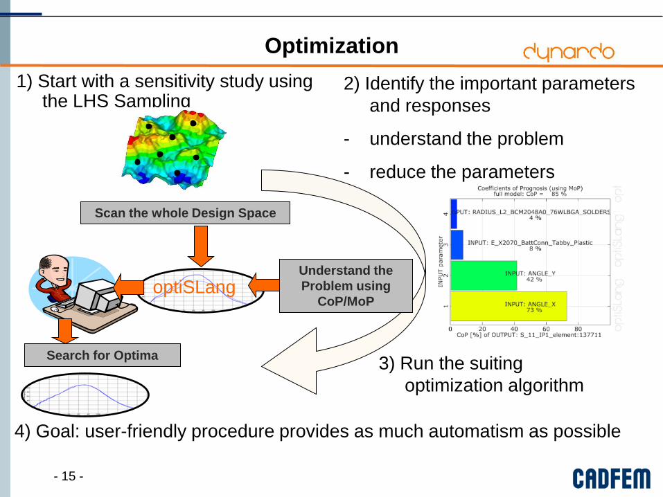
1) Start with a sensitivity study using the LHS Sampling
4) Goal: user-friendly procedure provides as much automatism as possible
3) Run the suiting
optimization algorithm
Understand the
Problem using
CoP/MoP
Search for Optima
Scan the whole Design Space
optiSLang
2) Identify the important parameters
and responses
- understand the problem
- reduce the parameters
Optimization
- 16 -
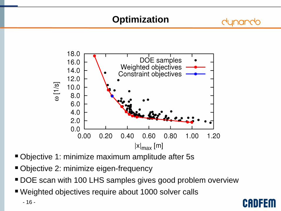
Objective 1: minimize maximum amplitude after 5s
Objective 2: minimize eigen-frequency
DOE scan with 100 LHS samples gives good problem overview
Weighted objectives require about 1000 solver calls
Optimization
- 17 -
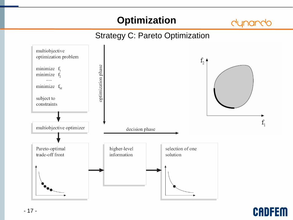
Strategy C: Pareto Optimization
Optimization
- 18 -
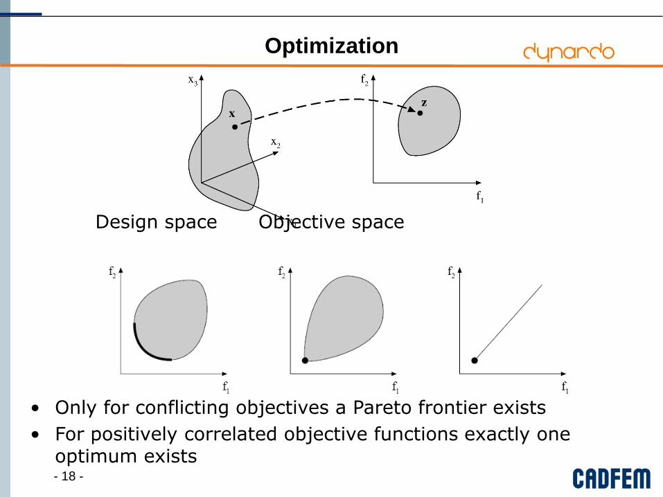
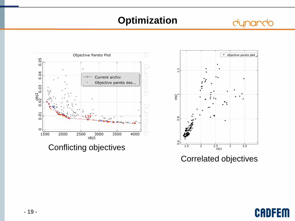
Design space Objective space
• Only for conflicting objectives a Pareto frontier exists
• For positively correlated objective functions exactly one optimum exists
Optimization
- 19 -
Correlated objectives
Conflicting objectives
Optimization
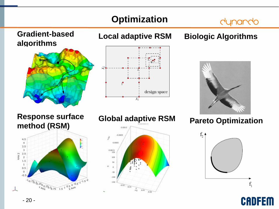
- 20 -
Gradient-based
algorithms
Response surface
method (RSM)
Biologic Algorithms
Start
Pareto Optimization
Local adaptive RSM
Global adaptive RSM
Outlook
Understand your Design
PRACE Autumn School 2013 - Industry Oriented HPC Simulations, September 21-27,
University of Ljubljana, Faculty of Mechanical Engineering, Ljubljana, Slovenia
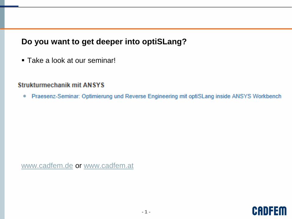
Do you want to get deeper into optiSLang?
- 1 -
Take a look at our seminar!
www.cadfem.de or www.cadfem.at

Tomorrow
- 2 -
Your feedback!

More Information?
Brochures
Feedback Form
Contact Information 0800-1-CADFEM
0800-1-223336
www.cadfem.de