Underreaction to Self-Selected News Events: The Case of Stock Splits

David L. Ikenberry Jones Graduate School of Management

Rice University Houston, Texas

daveike@rice.edu

Sundaresh Ramnath McDonough School of Business

Georgetown University Washington, DC

ramnath@gwu.edu

November 1999 This Version: July 2001

We appreciate the comments we received from Brad Barber, Will Goetzmann, Gustavo Grullon, John Heaton (the editor), George Kanatas, Jason Karceski, Roni Michaely, Raghu Rau, Jay Ritter, Kay Stice, Richard Thaler, Sheridan Titman, Kent Womack and seminar participants at the Review of Financial Studies Conference on Market Frictions and Behavioral Finance, April 2000, the NBER Behavioral Finance Meetings, May 2000 and the FMA European Conference, May 2000. We also thank Eugene Fama and Ken French for providing us with factor returns and I/B/E/S International Inc. for providing analyst forecast data. Scott Baggett was extremely helpful with data support. This paper was previously titled "Underreaction."

Underreaction to Self-Selected New Events: The Case of Stock Splits

Abstract

In the last decade, an emerging body of research looking at self-selected, corporate news events concludes that equity markets appear to underreact. Recent theoretical papers have explored why or how underreaction might occur. However, the notion of underreaction is contentious. Concern has focused on two issues - spurious results from unusual time periods and/or misspecified return benchmarks or methods. In this paper, we revisit the issue of underreaction by focusing on one of the most simple of corporate transactions, the stock split. Prior studies that report abnormal return drifts subsequent to splits do not appear to be spurious, nor a consequence of misspecified benchmarks. Using recent cases, we report a drift of 9% in the year following a split announcement. We consider fundamental operating performance as a source of the underreaction. Splitting firms have an unusually low propensity to experience a contraction in future earnings. The evidence suggests that investors underreact to this information. Analyst earnings forecasts are comparatively too low at the time of the split announcement and appear to revise sluggishly over time, a result consistent with underreaction by markets to corporate news events. JEL classification: G14, M49

1

The mechanism through which information is transmitted into stock prices has come under scrutiny

in recent years. Early foundations of modern finance presumed that the valuation impact of news was

transmitted to the market through buyers and sellers revising their expectations about future firm

performance. Any revision in expectations, in turn, changes the risk-adjusted value of the firm, which

through trading is eventually reflected in market prices. This transmission mechanism was argued to

operate in both a rapid and unbiased manner and motivated the term “efficiency.” Of course, the notion of

informational efficiency has never suggested that markets are somehow clairvoyant. No supposition is

made as to the absolute degree of precision with which prices should respond to news in any one case.

Indeed, because of the continual noise prevalent in markets, one cannot be surprised to find spurious

indications of pricing error in many situations, even when, on average, expectations, and thus prices

completely react to news.

However in the last decade, a broad-class of papers challenges the notion of informational

efficiency. These papers question the completeness of the immediate market reaction to corporate news

events. An extensive body of empirical literature examines a wide-ranging set of specific news events and

finds, with rather striking consistency, that markets appear to initially underreact. While not true in all

cases, positive news events are generally met with a positive market reaction. In these cases, returns

subsequent to the announcement show positive, long-horizon abnormal drifts. Similarly, negative news

events are generally met with a negative market reaction and tend to be followed by negative drifts.

While numerous concerns have appropriately been raised about the power or quality of these

empirical studies, the primary objections that strike to the core of this literature typically fall in two broad

areas. First, these papers reiterate concern over becoming errantly excited over spurious results. Given our

bias as researchers to explore interesting findings, we run the risk of collectively mining data and

circulating spurious findings when in fact this research commits a type one error; rejecting the null when in

fact it is true (Merton (1985)). A second over-arching criticism is that the mounting evidence of

underreaction is due to the absence of a robust asset-pricing model. In recent years, researchers have been

thrust into using ad-hoc models that, while having power in explaining cross-sectional stock returns, have

2

limited theoretical justification. These models take a variety of forms. Without guidance from theory, one

is left to question whether these ad-hoc approaches address all systematic sources of risk; a concern that for

the true skeptic can never be fully assuaged. Thus arises the famous joint-test hypothesis problem.

To some extent, this concern is reduced when the entire portfolio of underreaction events is

assembled. Here, the benchmark problem becomes one of suggesting that not one, but perhaps several still

unknown factors with cross-sectional power have extreme shifts in exposure that somehow affect returns in

a way that only gives the appearance of underreaction. Responding to these concerns is not always

straightforward. A conservative approach has been to account for as many factors as possible that, to date,

have demonstrated power in explaining returns. While this approach conceivably errs in “over-explaining”

the sources of returns to various factors (Loughran and Ritter (2000)), it does address whether any observed

drift can at least be characterized by known empirical relations.

In this paper, we examine this broad question of underreaction by narrowly focusing on the case of

stock splits. Of all the possible corporate events where researchers have observed potential underreaction,

this particular announcement is perhaps most interesting because of its utter simplicity. Unlike most

corporate news events, the split announcement is one situation where the event itself has little or no causal

properties that affect the firm in any material way. As such, the impact of a stock split is restricted to the

domain of investor expectations about future performance. By following a cleaner type of information

event, we hope to focus attention on the extent of underreaction and be less distracted by concern over

changing cash flows or risk characteristics perhaps caused by the event itself. Among the various

announcements one might consider, stock splits are rather unique in this regard.

Previous papers report some evidence of anomalous long-horizon returns for splits announced in

the 1970s and 1980s. In this paper, we look at out-of-sample results that focus on cases from the 1990s. To

measure abnormal performance, we use a rank-order search technique which tries to closely match one

control firm to each split firm on the basis of market-cap, value/growth, and momentum. To address

concern about liquidity, we also control for nominal share price levels.

We find that the positive drift in stock returns reported in previous studies does not appear to be

3

spurious. Using stock splits from 1988 through 1997 announced by NYSE, ASE and NASDAQ firms, the

drift following a split announcement during the 1990s is strikingly similar to results reported for earlier time

periods. Over the year following a split announcement, the mean match-adjusted abnormal return for

sample firms is 9.00% (t=7.93). The overall median abnormal one-year return is 6.31% (p<.0001)

suggesting that the post-split drift is not a consequence of a handful of right-skewed returns. These findings

are generally stable across various dimensions and are not focused only in smaller, less widely traded

stocks. For example, while mid-cap and small- stocks show evidence of positive drift, even large-stocks

show some evidence of drift. Moreover, the results do not appear to be too sensitive to momentum.

Between value and growth stocks, no real pattern in abnormal performance is evident.

Investors would appear to be underreacting to the news of a stock split. But what are they

underreacting to? We consider two issues. First, we evaluate whether underreaction to splits can be

attributed to investors failing to anticipate new analyst coverage, coverage that often casts the firm in a

favorable light. We find that while analyst coverage does increase after a stock split, this increase is no

different than the “normal” increase in analyst coverage for firms of similar size and with similar return

histories. Next, we consider whether the underreaction evident in returns may be due to investors who are

slow to revise their expectations about future operating performance. To do this, we evaluate the earnings

expectations of Wall Street analysts. Presumably, these astute observers of financial information have

incentives to revise their earnings forecasts to reflect whatever information a stock split might convey. If

markets are slow to revise their expectations of future performance after a stock split, one would

hypothesize that analysts’ earnings forecasts will also revise slowly, in a manner consistent with the

subsequent sluggish price performance observed in previous studies. Conversely, to the extent that flawed

return benchmarks are the culprit, one hypothesizes that earnings expectations should be unbiased.

Focusing on earnings expectations, we again find evidence consistent with underreaction. Firms

that announce stock splits tend to have high earnings growth. However, even though this growth rate is on

average about three times greater than that of the overall economy, it is only marginally higher than what

we see for matching control firms. The distinguishing feature of splitting firms is a comparatively low

4

propensity for earnings declines, a result consistent with some of the stories we see for why managers

choose to split their shares. Overall, analysts do not appear to incorporate this information into earnings

forecasts when firms announce splits. We focus on forecasts pertaining to the next release of annual

earnings and observe how this forecast changes after a split announcement. We find that ten-days before

the split announcement analysts tend to underestimate future earnings of splitting firms relative to that of

their control firms by -7.67% (p<.0002). Ten-days after the split announcement, this gap drops slightly to

-7.08% (p<.0001). Over the next few months, expectations for the split and match firms converge toward

their actual values. However, even three days prior to the actual earnings release, earnings expectations for

the split firms are still too low by -2.68% relative to the expectations of matched control firms. This finding

is robust across various groups of stocks and does not appear to be driven by analysts making concurrent

mistakes on an industry-wide level.

Later in the paper, we perform a variety of robustness checks. We consider risk and statistical

significance issues, and also examine whether dividend changes around split announcements may be

affecting our conclusions. We also investigate the post-split drift using a separate estimation technique and

greatly expand our sample to incorporate announcements from as early as the 1930s. None of these

additional checks has a material impact on our conclusions. In short, the evidence, at least with respect to

stock splits, is consistent with the notion that markets underreact to firm-specific news. Our finding of

underreaction by Wall Street analysts is consistent with new theoretical papers, such as Barberis, Shleifer

and Vishny (1998) which try to motivate how or why markets might underreact. For example, Daniel,

Hirshleifer and Subrahmanyam (1998) model how analysts might overweight their own priors when valuing

firms, and thus underweight new information, like split announcements for example.

The balance of the paper is organized as follows. In section I, we briefly review the evidence on

underreaction and motivate our choice in this study to revisit the evidence on stock splits. Section II

discusses the sample and how we identified matching control firms. Section III reports evidence on long-

horizon abnormal returns after split announcements. In Section IV, we consider two potential sources of

fundamental news or information that might account for at least part of the apparent drift. In section V, we

5

provide some robustness checks and in section VI, we summarize the paper.

I. The evidence on market underreaction and our focus on stock splits

Over the last decade, the empirical literature on long-horizon stock returns has grown substantially,

much of it focusing on corporate news events. Generally speaking, firm-specific events can be sorted into

two classes. The first set consists of self-selected events where corporate insiders choose to execute a given

transaction at a particular point in time. This class of events is interesting because the joint decision of both

if and when to execute a given transaction is at the discretion of management, individuals who may have

private insight into the firm’s true value and future prospects. The second class of events is non-self-

selected. The timing and execution of these events is at the discretion of outsiders to the firm. Although

these events may be motivated by decisions insiders may have previously made, they are not specifically

conditioned on management's knowledge about the firm. While long-horizon return drifts have also been

document after non-self-selected events, we focus attention here on self-selected events because of their

endogenous nature.

Among the set of self-selected events, one of the earliest papers to examine long-horizon

performance that received widespread attention was Ritter (1991). That paper reports that managers

appeared to be “timing” the market at a relative peak when initially issuing equity as subsequent long-

horizon abnormal returns were negative. Subsequent studies by Loughran and Ritter (1995) and Spiess and

Affleck-Graves (1995) reported similar long-horizon findings for seasoned equity offerings. Because

market prices could be measured prior to this type of offering, the evidence leaned further toward

managerial timing and market underreaction to the news of an offering. In fact, aggregate flows of equity

offerings appear to have predictive power for overall market returns (Baker and Wurgler (2000)), thus

giving some merit to the notion of the “window-of-opportunity” when companies choose to issue stock.

The transaction that complements equity offerings is an equity repurchase. Lakonishok and

Vermaelen (1990) examine long-horizon returns subsequent to fixed price tender offers. For the more

common open market stock repurchase transaction, Ikenberry, Lakonishok and Vermaelen (1995 and 2000)

report long-horizon return evidence in the U.S. and, more recently, in Canada. These papers find that for at

6

least repurchases, managers seem just as sensitive to underpricing as their counterparts seem sensitive to

overpricing.

Another self-selected event concerns the initiation of dividends where managers may be signaling

confidence. Here, Michaely, Thaler and Womack (1995) find evidence of positive drifts subsequent to

dividend initiations. Another self-selected event is the spin-off; a transaction often motivated to “unlock”

value that is otherwise not priced by the market. Desai and Jain (1999), Cusatis, Miles and Woolridge

(1993) and Miles and Rosenfeld (1983) find evidence of positive drifts subsequent to these announcements.

The list of negative return drifts where managers may be responding to perceived over-pricing, is

also substantial. These events are also self-selected, yet theoretical stories about managers choosing to

intentionally signal information, of course, carry much less significance. An early paper in this area is

Agrawal, Jaffe and Mandelker (1992) who report negative long-horizon abnormal returns following

mergers. More recently, Loughran and Vijh (1997) and Rau and Vermaelen (1998) extend this work and

find that these negative drifts are associated with equity deals, particularly those done by growth companies

where managers may be using "overvalued" stock as currency in a given transaction. Other negative self-

selected events include dividend omissions (Michaely, Thaler and Womack (1995)), and exchange listings

where firms (particularly small- and mid-cap firms) move from one trading market to another (Dharan and

Ikenberry (1995)). Recently, new evidence suggests that managers may also be timing the issuance of

straight and convertible bonds (Lee and Loughran (1998), and Spiess and Affleck-Graves (1999)).

Why the focus on stock splits in this paper? Stock splits, of course, are another self-selected

corporate event that managers control. Yet among the class of self-selected events, stock splits are

appealing because they are one of the few decisions that seemingly has no direct impact on either cash

flows or firm risk. By contrast, nearly all corporate transactions are, by design, intended to have potentially

dramatic effects on operating cash flow, capital structure, internal capital allocation, managerial incentives

or tax liabilities for example. Because of the dynamic changes these events cause, concern may exist as to

how well and/or how quickly the market can digest this more complex information. Furthermore, concern

naturally exists as to what impact these events may have on risk and thus expected returns, a sensitive issue

7

for studies dealing with measuring long-horizon performance.1 Stock splits are intriguing because their

direct impact on the firm is seemingly negligible.

While debate continues as to why managers split their stock, the question of interest here is whether

the initial market reaction to whatever news might be associated with splits is unbiased and complete. The

earliest empirical study in this regard, Fama, Fisher, Jensen and Roll (1969), suggested that the answer

might be yes. Studies in the mid-1990s, relying on more recent empirical methods (Ikenberry, Rankine and

Stice (1996) and Desai and Jain (1997)), suggest that the initial market reaction may not be so unbiased.2

Some researchers have expressed reservation about evaluating long-horizon returns casting doubt as to the

robustness of this literature (Mitchell and Stafford (2000)). The drift evident following splits has been

viewed with a degree of suspicion as well (Fama (1998)).

In this paper, we take a deeper look at the evidence with respect to stock splits and address at least

some of these concerns. We also consider data more directly related to the notion of underreaction, namely

analysts’ expectations.

II. Sample and Methods

a. Sample

We begin our examination in 1988, the first year that the I/B/E/S Details Tapes have rich cross-

sectional coverage. Return data is obtained from the CRSP tapes ending on December 31, 1998. Thus, we

stop with announcements made in 1997 so that we can measure a full-year of returns after the split

announcement. From 1988 to 1997, the population of stock splits of 5-for-4 or greater announced by

1 Recently, the negative drift subsequent to equity offerings has come under reexamination. Eckbo, Masulis and Norli (2000) argue that the new-issue puzzle surrounding equity offerings arises because this particular transaction reduces leverage-risk and improves trading liquidity. To the extent that these two factors are priced, it may lower the required return for these types of firms. Similar arguments might also be made for a wide variety of transactions that affect either operating cash flows or financial characteristics of the firm. This should be less of a concern here. It is not clear why managers would voluntarily agree to a seemingly unnecessary action if it somehow caused their cost of capital to increase. Furthermore, if splits did somehow cause the cost of equity to increase, it raises suspicion as to why the initial market reaction is uniformly positive, instead of negative as one might otherwise expect. 2 Prior to these studies, Grinblatt, Masulis and Titman (1984) also report evidence of unusual post-split return performance.

8

NYSE, ASE and NASDAQ firms totals to 4,154 cases.3 From the total population, 3,028 cases had data

sufficient for conducting our matching procedures.4 Although the time period we examine overlaps with

previous work by Ikenberry, Rankine and Stice (1996) and Desai and Jain (1997), the final six years in this

sample (1992-97) have not been evaluated in previously studies and thus serve as a convenient hold-out

sample. Table 1 shows the number of cases by year and by split factor. Split factors of two-for-one or

more comprise roughly half the sample. Moreover, there is a slight tilt toward more recent observations.

b. Methods

We measure post-split abnormal returns using a buy-and-hold approach, comparing the return to

splitting firms to that of a single control-firm (Barber and Lyon (1996 and 1997)). To find a match for a

given sample firm, we form a candidate pool by first identifying all firms that as of a given month had not

split their stock in the previous year. We then locate a match by controlling for market-cap, value/growth,

and momentum using the following procedure. First, using the market value of all NYSE firms at the end

of the month prior to the split announcement, firms are assigned to one of five market-cap quintiles. Each

market-cap quintile is further divided into five more quintiles based on the prior 36-month return of the

firms in each group. And finally, within each market-cap by three-year return group, firms are further

classified into quintiles based on their 12-month return prior to the split announcement. Once these NYSE

cut-off values are defined for a given month, all public firms trading at that time, including our split firms,

are classified into one of these 125 (5x5x5) characteristic portfolios.

To identify our one matching firm, we start by considering all the firms classified in the same three-

factor characteristic portfolio as the splitting firm. To narrow this set down, we then control for potential

differences in liquidity. Each month we estimate the distribution of nominal stock prices using only NYSE

3 One might question why we also do not consider stock dividends as these events are often viewed as mini-versions of stock splits. It is not clear that this really is the case. The accounting treatment for the two procedures is quite different. Stock dividends can dramatically decrease a firm’s retained earnings balance and thus affect numerous accounting ratios, performance metrics and covenants. Splits have no such impact (Grinblatt, Masulis and Titman (1984) and Rankine and Stice (1997a)). Moreover, there is evidence that the market responds differently when managers are given the chance to choose between the “easy” accounting treatment afforded stocks splits as opposed to the “hard” treatment that stock dividends receive (Rankine and Stice (1997b)). 4 Most of the firms lost at this stage were young firms having less than 36 months of observations prior to the split announcement.

9

stocks and eliminate all potential matches whose price is not within 5 percentiles of our sample firm's post-

split price.5 Next, we use a rank order procedure. All eligible candidates at this point are ranked from 1 to

n (n being the number of eligible matches) based on the closeness in value between the sample and the

match firm on each of the three matching dimensions (market-cap, three-year return, and one-year return).

Ranks are summed across all three categories and the firm with the lowest cumulative sum is picked as the

match firm for a given splitting firm. If for any reason the first match becomes ineligible at a given point in

time (for example, if it ceases to trade or it too announces a split), the firm with the second lowest sum of

ranks is used from that point forward, and so on. This procedure ensures that there is no look-ahead bias.

Our basic approach to forming benchmarks is worthy of some discussion. First, we adjust for

intermediate (one-year) price momentum. Jegadeesh and Titman (1993) report compelling evidence about

the explanatory power of this form of momentum. Yet it is not entirely clear that one should make such an

adjustment in a study about underreaction. For example, Chan, Jegadeesh and Lakonishok (1996) conclude

that price momentum can and should be interpreted as underreaction by the markets to news in earlier

periods that is only gradually being corrected over time. On the other hand, splitting firms load exceedingly

high on momentum.6 Not controlling explicitly for this, of course, would raise nagging suspicion as to

whether the long-horizon evidence following split announcements is not simply a general manifestation of

momentum. We choose to err on the conservative side and estimate abnormal returns controlling for

momentum. Thus one might choose to interpret our evidence of underreaction to split announcements as

net of the drift “normally” apparent in firms with high momentum.

A second issue relates to our use of the three-year stock return preceding the split announcement as

a proxy for the value/growth factor. A traditional approach here is to use book-to-market. However, book

equity values tend to change slowly overtime. The greatest source of cross-sectional variation in B/M ratios

5 A further benefit of matching on post-split price is that the match firm itself is less likely to be a candidate to split its own stock in the near future. 6 Excess returns in the preceding year tend to be extreme; the median, for example, is roughly 50%.

10

is clearly due to variability in preceding returns. For example, Lakonishok, Shleifer and Vishny (1994)

show compelling evidence of the relation between B/M and trailing three-year returns. Moreover, sorting

on historical returns instead of accounting ratios has some appeal in our setting. First, this approach allows

us to assume that investors are forming portfolios using simple and generally available information.

Second, this approach also removes IPOs from the split sample. More importantly, it eliminates IPOs from

the pool of potential matching control-firms until these firms have at least three years of seasoning. And

finally, this approach also allows us to consider stock splits from time periods as early as the 1930s where

accounting information is not readily available.

Table II presents descriptive statistics for sample and control firms along the various matching

dimensions. Overall, the split and control firms appear to match fairly well and show no particular

discrepancy. Stock split announcements are distributed over all market-cap quintiles. Not surprisingly, we

see that stock splits tilt in favor of high growth and high momentum.

III. Long-horizon abnormal stock return evidence

a. The overall evidence

Table III reports one-year abnormal returns for the overall sample of 3,028 split announcements.

The mean total return for sample firms is 23.29%. This contrasts with the total return for the matched-

control firms of 14.29%. This difference of 9.00% (t=7.93) is roughly double the risk premium typically

associated with stocks relative to bonds. Here, we estimate significance using a t-test, an approach that is

generally robust for one-year abnormal returns using a single matching-firm approach (Lyon, Barber and

Tsai (1999)). While random collections of firms should not be expected to have dependent errors, self-

selected samples may well be different. To the extent that our underlying asset-pricing model is incomplete

our significance may be overstated, thus some degree of caution is warranted. Later in section V.b, we re-

examine this issue.

Long-horizon returns tend to exhibit positive skewness. While the matching firm approach

mitigates this issue (Barber and Lyon (1997)), we nevertheless consider two approaches to reduce the

impact of outliers on our analysis. A simple technique is to examine median returns. Median returns pose a

11

problem when considering questions of efficiency because of the inconsistency this statistic poses for ex-

ante trading strategies. However, medians allow some sense of robustness and thus we consider them here.

The overall median paired difference is 6.31% and the p-value for the Wilcoxon signed-rank test is less than

.0001.7

Other approaches for handling skewness involve some ex-post alteration or truncation of the data.

Such an ex-post remedy does not reflect the performance that investors could generate ex-ante and, as such,

again is not consistent with our objective here. Thus we consider an alternative method that is consistent

with a real-time strategy, which we label as real-time truncation. Here we monitor, on a daily basis from

the initial investment date, the excess compounded return for each split firm relative to its paired-match

firm. At any given point in time when that paired difference exceeds 100%, we assume that the position is

liquidated and the return for the remainder of the year is set to 0%. Using this ex-ante approach, we cap our

extreme winners, yet we retain all the losses that might be generated from extreme, right-skewed returns

coming from a short position in the matched control-firm. As a final check, we also report ex-post evidence

that assumes trimming extreme high and low abnormal returns to their respective 99% and 1% values.

The evidence using both the real-time truncation approach as well as the winsorized results is

similar. Removing only the extreme winners under the real-time truncation approach does not materially

affect the results. The point estimate of the mean abnormal return falls slightly from 9.00% overall to

8.26%, although by eliminating extreme winners statistical significance is roughly the same.

b. Consistency

In this section, we report abnormal performance for various partitions of the sample to examine the

consistency of the positive drift. We begin with Table IV by reviewing the evidence across various years in

our sample, across the three trading markets and finally by the various split factors.

Our sample starts in 1988 and thus overlaps with evidence reported by Ikenberry, Rankine and Stice

(1996) whose sample ends in 1990 and also with that of Desai and Jain (1997) whose sample ends in 1991.

7 Because of the non-parametric nature of this approach, the median paired difference in returns does not equate to the difference in median total returns for splitting and matching control-firms separately.

12

Both studies find evidence of positive drift during the first year after a split announcement. We see

confirming evidence of this in the first panel of Table IV for the sub-periods 1988-89 and 1990-91.

However, we also see positive drift in each of the subsequent sub-periods as well. Apparently, the drift

observed in previous studies for splits in the 1970s and 1980s is not unique. There is little evidence that the

drift is receding over time. In fact, the mean and median abnormal returns for the most recent period, 1996-

97, are similar to the respective mean and median numbers for the entire ten-year period.

The drift is similar for both ASE and NYSE firms, 7.36% (t=2.02) and 7.63% (t=5.05) respectively.

For NASDAQ stocks, the point estimate is a little higher,10.27% (t=5.90). One concern might be that our

matching approach somehow does not adequately control for differences in returns across exchanges.

Reinganum (1990) points out that returns to NASDAQ stocks are generally lower than similar NYSE

stocks, thus posing concern about inflated abnormal returns for some of the non-exchange matched NYSE

firms. However, Loughran (1993) points out that much of this inter-market difference is driven by the

comparatively higher prevalence of initial public offerings among NASDAQ stocks. Fortunately, we

impose a three-year seasoning requirement on both sample and matching control firms and thus mitigate at

least a portion of any exchange bias.

In the third panel, we see that abnormal performance is evident across the various split factors.

Two-for-one splits are the single most prevalent split factor in our sample and show the lowest point

estimate for mean abnormal performance, 6.75% (t=3.94). Split factors less than and more than two-for-

one show mean abnormal performance of 10.40% (t=6.58) and 13.74% (t=2.66) respectively.

In Table V, we examine the evidence across the same dimensions that we initially controlled for

when identifying matching control-firms. While one can never fully allay questions about the quality of the

benchmark, we can at least examine whether our findings are driven by a limited number of factors. The

first sub-panel reports abnormal returns by market-cap quintile defined relative to only NYSE stocks.

While mean and median abnormal performance is indeed positive and significant for the smaller three

quintiles, abnormal performance is not limited to only small firms, a concern voiced in the literature in

recent years. For example, even the largest firms in our study (stocks we often consider to be extensively

13

followed and traded by institutional investors) show some evidence of abnormal performance; the mean

abnormal return for large-cap quintile 5 stocks being 4.42% (t=2.25).

Firms that announce stock splits overwhelmingly are classified as growth stocks. In our case,

roughly two-thirds of the sample is classified in the highest growth quintile. Not surprisingly, the mean and

median abnormal performance for quintile 5 is comparable to that observed for splits in general. Moving

toward the other extreme, sample size declines rapidly; thus our estimates of abnormal performance for

these quintiles are noisy. Nevertheless, the point-estimates suggest a positive drift throughout the value-

growth spectrum.

Firms that announce stock splits tend to have high one-year return momentum. These cases are

interesting to examine for these stocks are often in the news and draw attention from both investors and

analysts. Thus, one might expect to find excess performance primarily in the low momentum quintiles.

Yet, abnormal returns are greatest in the high-momentum quintiles 4 and 5 where mean abnormal returns is

10.28% (t=5.30) and 10.12% (t=5.02) respectively.

IV. The Source of the Underreaction

The evidence suggests that investors are underreacting to the news of a stock split. In this section,

we investigate two possible fundamental sources of this news. One branch of the literature on splits

suggests a well-known and appreciated story that managers may use splits to intentionally convey news to

the market (Brennan and Copeland (1988a)). One example is Brennan and Hughes (1991) who argue that

managers may use splits to draw increased analyst attention. For example, if trading costs increase after

stock splits, managers who want increased analyst coverage might choose to split their stock. Moreover,

McNichols and O'Brien (1997) point out that new coverage is generally favorable. This is consistent with

the reasoning in Schultz (2000) that stocks may benefit from increased “promotion” after a split. If

investors are, for some reason, slow to anticipate this outcome, it is plausible that the long-horizon drift may

be due to investors reacting to unanticipated analyst enthusiasm as time passes after a stock split.

A second branch of literature offers that the source of the underreaction is more fundamental in

nature. These papers suggest that the post-split drift may simply be due to the market only gradually

14

revising its expectations about future earnings. Several papers (e.g. Grinblatt, Masulis and Titman (1984),

McNichols and Dravid (1990) and Ikenberry, Rankine and Stice (1996)) argue that managers may condition

stock splits on expected future earnings. Managers considering a stock split, but who are not pessimistic

about future operating performance, voluntarily self-select and proceed with the event. Yet managers who

are pessimistic may be less likely to split, particularly if either they or the firm bear some penalty if prices

fall below a certain level. Thus, managers choosing to split their shares may be signaling, either directly or

indirectly, their optimism about future operating performance. Clearly, this story is consistent with the

positive market reaction that stock splits receive at the time of their announcement. The issue, though, is

whether this reaction is complete. If investors are slow to incorporate the implicit signal from managers,

then we should see abnormally low earnings expectations at the time of the announcement. Moreover, we

would expect to find that these forecasts are revised upward on average over time.

To examine these potential sources of underreaction, we begin by looking at all stocks in our

sample that are followed by analysts. We then evaluate their forecasts around the time of the stock split and

also examine revisions subsequent to the split announcement. Of course, analysts’ forecasts for next year’s

earnings are but one element in the future stream of cash-flows that investors need to consider, and thus are

probably not a perfect proxy for the market’s overall expectation about the future. Yet, analysts’ earnings

forecasts clearly affect market prices (Womack (1996)). Moreover, these analysts are conceivably engaged

in providing some indication of future performance. Perhaps using this data, we can objectively evaluate

whether this subset of influential market participants shows any systematic bias in its expectation of future

operating performance and, if so, see whether it is consistent with the drift evident in stock returns.8

We form a sub-set from our original sample by looking for cases where both the split firm and its

corresponding match have earnings forecasts available on I/B/E/S for the next fiscal year-end. In cases

where the next annual earnings announcement is within 125 trading days of the split announcement

8 Of course, we are not the first to consider these issues. Several papers, including Lakonishok and Lev (1987) and McNichols and Dravid (1990), report evidence on earnings growth and earnings expectations following stock splits. We extend this work by also considering the evolution of expectations subsequent to split announcements.

15

(roughly six calendar months), we jump ahead to the following fiscal year. This requirement provides us

with at least some time to examine the evolution of earnings forecasts after the split announcement.

From our original dataset, we find 948 firms that satisfy the I/B/E/S data requirements. For this

group, we obtain their earnings in the fiscal year prior to and following the stock split normalized by price

at month-end prior to the split announcement. We use actual operating earnings before unusual items as

reported by I/B/E/S, a number more consistent with what analysts are trying to forecast.

a. The increased analyst attention hypothesis

Do stock splits lead to increased following by financial analysts? This evidence is summarized in

Table VI for both split and match firms. Overall, we see that analyst coverage following a stock split for

our sub-sample of 948 firms does indeed increase from a median following of 9 analysts just prior to the

split to 13 analysts three days before the subsequent annual earnings announcement. However, a similar

pattern is evident in our matching control-firms. Although we did not specifically match on earnings levels

or analyst coverage, we see that matching firms have roughly the same number of analysts and the same

growth in analyst following as the split sample measured at the same points in time. It is not clear that the

split itself has any marginal impact in drawing added coverage. Instead, the increase in analyst coverage for

splitting firms may simply be more a consequence of how analysts choose to cover new stocks.

b. Slowly revising earnings forecasts

Next we consider the issue of whether the market may be slow in revising its forecast of future

earnings growth. We begin by considering how actual earnings are changing in our sample firms. Later,

we focus on earnings expectations and how they evolve over time.

Table VII reports growth in realized earnings yield from the year prior, to the year following the

split announcement for our sub-sample of firms. Split firms are doing well around the time of a stock split.

The mean change in earnings yield around a split announcement is 1.18%, implying growth in absolute

earnings of about 20%. Further, nearly 85% of split firms show positive earnings growth. Interestingly, the

matched control firms (again, which are not intentionally matched on earnings growth) also seem to be

doing well. Here, the mean matching firm shows earnings yield growth of .92%, and 73% of these cases

16

are positive. For both sets of firms, earnings growth is strong, yet the difference between the two groups is

not so impressive. While, the mean difference in earnings yield growth is .26% and marginally significant,

the median difference is lower at .14% with only slightly more than half the paired differences being

positive. This result is consistent to some extent with Lakonishok and Lev (1987). They form control firms

on the basis of industry and size and also report only a modest difference in earnings growth between a

sample of split and control firms.

Yet both splitting and matching control firms together are experiencing unusually high earnings

growth. For comparison, we report the concurrent growth in earnings yield evident in the S&P industrial

index matched in time to each of our cases. Here, we see a more compelling case for earnings growth.

Overall, mean earnings growth for both sets of firms is roughly three times the rate of growth observed in

the market overall. Although firms announcing splits have unusually high earnings growth, this growth is

not particularly excessive when compared to firms of similar size and with similar prior return histories.

While the mean change in earnings between both sets of firms is similar, an interesting question to

consider relates to the stories suggested in the literature about why we even see splits at all. For example,

stock splits may not be a signal of abnormal growth in future operating performance, but rather managers

may use splits when they sense confidence that past earnings growth is not likely to erode (Asquith, Healy

and Palepu (1989)).

This suggests that the distribution of earnings changes in our two samples may differ in a more

subtle way than is evident from looking only at mean and median changes. We consider this issue more

carefully by plotting the distribution of changes in earnings yield for both sample and match-control firms

in Figure 1. Focusing on the right side of this graph, we see little difference between the two distributions.

In fact, over only the high growth region above 2%, the cumulative density for matching firms is slightly

greater than that of splitting firms. Clearly, splitting firms are not demonstrating unusually skewed

operating performance. Instead, the apparent difference between the two distributions is due to a relative

absence of negative growth realizations in the split sample. This mass is shifted slightly to the right near the

overall mean. Thus for splitting firms, we see an extremely high density of earnings yield changes in a

17

range between .5% and 1.5%. A two-sample Kolmogorov-Smirnov test easily rejects the hypothesis that

these two distributions are the same with a p-value well below 1%. As a further check, we can recenter

both distributions to mean zero to take into account that the mean growth rate between the two groups

differs. Even with this more stringent test, we still reject with p-values below 1%. In short, it would appear

that managers announcing splits may not be anticipating a rapid acceleration in earnings so much as they

sense a low likelihood of a decline in operating performance. With reduced concern that future stock prices

will trade below some desired minimum, managers may have the confidence to split their shares to a lower

“trading-range.”

Next, we shift attention to forecasted earnings and consider whether the market anticipates how

earnings change when firms announce a split. We examine the earnings forecasts for sample and match-

control firms at various points around the split announcement but prior to the release of next years’ annual

earnings. For most split and match-firm pairs, the respective earnings announcement dates fall within a few

days of each other, however they are not perfectly aligned in calendar time. We align the two groups in

event time by choosing a “pseudo-split date” for the match firm which is the same number of trading days

prior to its earnings announcement date as the sample's split announcement date is from its earnings

announcement.

Forecasts for sample and for match-control firms are expressed as a percentage of the actual

(subsequently realized) earnings. At various points in event time, we compute one forecast accuracy

measure for sample firms and a separate measure for control-firms. This measure is as follows:

∑

∑

=

== n

iti

n

iti

tI

PA

PFFPA

1,

1,

,

)/(

)/( (1)

where FPAI,t is the forecast at time t for group I (I = sample, match) expressed as a percentage of the actual

earnings for group I. (F/P)i,t is the forecasted earnings per share (EPS) for firm i at time t scaled by its stock

price as of the end of the month prior to the split, and (A/P)i,t is the actual EPS for firm i at time t scaled by

the same stock price. This approach allow us to form a summary measure of earnings growth using all

18

firms, including those that have unusually low or even negative levels of initial earnings (Givoly and

Lakonishok (1989), Ikenberry and Lakonishok (1993)).

Our measure of analyst bias is the difference in FPA between the split and match-control groups.

Here, the role of the control firm is important. If analysts had no bias in their forecasts, one would expect

the FPA for both groups at any point in time to be 100%. Yet recent papers including Easterwood and Nutt

(1999) and Richardson, Teoh and Wysocki (2000) show numerous departures from this naive baseline.

These papers find that historically, analysts’ forecasts tend to be high and gradually revise downward over

time as the earnings release date approaches. Moreover, this “game” is not uniform. It varies for small

compared to large stocks and also for growth compared to value stocks. Further, this forecast bias is not

stable over time. In short, we need to use matching-control firms to calculate an FPA-benchmark so that we

have some sense of the “normal” level of bias to expect in our sample. Conceivably, this bias is already

built into market expectations. Of course if there is no bias at a given point in time, this approach induces

no harm other than adding noise to our analysis.

To examine the statistical significance of the difference in FPAs between the split and control

samples, we use a randomization procedure. We assume under the null that both the split and its paired-

matching firm are jointly drawn from the same underlying universe. For each observation in our sample,

we randomly reassign one firm to the “split” group and the other firm to the “match” group. After

completing this for each observation, we have one trial formed under the null-hypothesis. We obtain an

empirical distribution by repeating this process for 10,000 trials. This gives us some sense of what the

distribution of FPA differences looks like if we assume no difference between splitting and control firms.

We then obtain p-values by comparing the actual FPA difference to the empirical distribution and record the

cumulative density. This procedure is executed separately for each FPA statistic, thus forcing each

empirical distribution to be consistent both over event-time and across sub-samples.

Results of this analysis are presented in Table VIII. Consistent with prior studies which find that

analysts' forecasts well in advance of an earnings announcement tend to be optimistic, we also find evidence

of optimism for the control firms. For example, EPS forecasts for our matching control firms are 5.50% too

19

high at the beginning of the event period. However over time, these forecasts come down such that they

exceed actual EPS by around 2.7% three days prior to the earnings announcement date. For splitting firms

on the other hand, the forecasting behavior is markedly different. Ten days prior to the split announcement,

analysts underestimate annual EPS for splitting firms by roughly -2.2%.9 Over time, the mean forecast

increases slightly, a result that contrasts with the general behavior of forecasts during this period.

The relative difference in FPA is our unit of interest. Here we see that the earnings forecast bias for

splitting stocks overall is -7.67% (p<.0002) measured two weeks prior to the split announcement. Two

weeks after the announcement, this error is still substantial, -7.08% (p<.0001). As we move forward in

time, the bias gradually declines. Forecasts for both splitting and matching-control firms converge

(although not completely) toward their actual EPS. If we sort the data by firm characteristic, we find that

the bias in analysts’ forecasts and their sluggish revision over time are not focused in any particular subset.

One question is whether analysts’ forecasts are flawed or biased because of some unanticipated real

change concurrently affecting the splitting firm’s entire industry. For example, firms might be splitting

because of generally improving industry-wide, economic conditions. If analysts were somehow failing to

anticipate these industry shifts in profitability, this might explain the bias we see in Table VIII. We

checked this possibility by replacing the matching firm with a value-weighted portfolio of all other

companies in the splitting firm’s industry. Details are provided in Appendix Table A. Applying this new

benchmark does not seem to affect the results. The bias we see in analysts' forecasts for splitting firms

cannot be attributed to unanticipated shifts in overall industry profitability.

Some portion of the underreaction to split announcements appears to be due to biased earnings

forecasts and the market’s propensity to revise its expectations slowly over time. We investigate this more

carefully by estimating the extent to which the cross-sectional variation in abnormal returns following splits

is explained by corresponding earnings forecast revisions. For this, we focus on the period beginning ten

days after the split and ending three days prior to the announcement of annual earnings. The match-

9 Using a different technique, McNichols and Dravid (1990) also report evidence of biased expectations when splits are announced.

20

adjusted return for splitting firms over this period is comparable to the one-year post-split returns presented

in Table III. In Panel A of Table IX, the mean differential return is 8.30% and the median return is 7.52%.

Turning to forecast revisions, we observe that both the mean and median match-adjusted forecast revision

for splitting firms is positive and significant.

Panel B of Table IX summarizes the association between the match-adjusted forecast revision

(MAFR) and the match-adjusted returns (MAAR) of the splitting firms from ten trading days after the split

announcement to three days prior to the earnings announcement. If the positive drift in the abnormal

returns of splitting stocks can be attributed to the biased earnings revisions following splits, b should be

positive and roughly equal to the average earnings capitalization factor (P/E ratio) in the following

regression:

eMAFRbaMAAR ii ++= * (2)

As expected, b is positive, 10.35, and significant. Moreover, the scale of b is not completely unreasonable.

The median E/P ratio of these splitting firms is roughly .06, suggesting a P/E of about 17. Thus, while our

point estimate is lower than we might expect, a host of other factors affect the dependent variable here.

Overall, the evidence suggests that at least some portion of the positive drift in the abnormal returns is not

entirely attributable to misspecified return benchmarks but instead can be explained by the gradual revision

in analysts' earnings expectations following split announcements.

V. Robustness The bias and subsequent revision we see in analysts’earnings forecasts is consistent with the drift

we also see in stock returns and supports the notion of underreaction. However, measuring long-horizon

abnormal stock returns is not straightforward and concern often exists as to the robustness of the evidence.

We address a few of these concerns here. First, we consider whether the unusually high returns following

stocks splits might be due to substantive changes in risk. Next, we investigate whether the true

“information” event is coming from a source other than splits. Specifically, we consider whether changes in

dividend policy might be driving our results. Next, we consider significance issues regarding the buy-and-

21

hold return evidence. And as a final robustness check, we discard the buy-and-hold approach altogether and

estimate performance using a calendar-time portfolio technique.

a. Risk changes around stock splits

A key feature that distinguishes splits from other corporate transactions is that this event is

seemingly innocent with no apparent potential to impact a firm's fundamental risk or its cash flows. On the

surface, there is little reason to question whether splits directly cause some change in the risk characteristics

of the firm. Thus if one thinks of the stock price as the sum of discounted future cash flows, the conclusion

would seem to be that the market is underestimating the numerator, the future cash flows (or earnings), at

the time of a stock split.

However a lingering question is whether the denominator, the discount rate, is also somehow

affected by a split. Specifically, one might question whether the post-split drift somehow results from a

material increase in market risk even though business fundamentals may not have changed. Several papers

have investigated this possibility and have observed that return volatility, including systematic risk, does

increase around the time of a stock split (Dubofsky (1991), Brennan and Copeland (1988b), and Ohlson and

Penman (1985)). A recent paper by Angel, Brooks and Mathew (1998) finds that this increase in volatility

may be due to changes in market structure arising from the new, post-split price regime and not to changes

in the fundamental flow of information. However, the evidence from this literature is not unambiguous. It

is also not clear how substantive or permanent the increase in risk actually is. For example, Wiggins (1992)

finds that the increase in risk is largely confined to a short period immediately following the split

announcement. Dubofsky (1991) also raises doubt as to the extent to which risk is fundamentally changing.

Moreover, these papers tend to focus on short-horizon estimates of risk using daily, or in a few cases,

weekly data. These estimates can be noisy and potentially prone to error.

We consider these issues by reporting various estimates of risk in the year prior to and following a split

announcement. We focus on monthly returns and use an Ibbotson (1975) RATS- type approach where

sample returns are aligned in event time and risk is estimated cross-sectionally. In Panel A of Table X, we

report total risk as measured by the cross-sectional standard deviation of returns. Consistent with prior

22

studies, we also detect an increase in total risk around split announcements. Yet this increase is modest in

scale and largely confined to the announcement month and the immediate surrounding months. Comparing

the pooled pre-split evidence with the corresponding post-split period, total risk increases from .116 to .119.

Digging a little deeper, we estimate systematic risk exposures month by month. Panel B reports

changes in market risk using a conventional one-factor market model. In Panel C, we use a Carhart (1997)

four-factor model that adds size, book-to-market and momentum factors. Again, consistent with previous

studies, one can detect a short-lived increase in systematic risk in the months surrounding the split.

Evidence of any permanent increase in risk is not so compelling. Using a one-factor model, market risk

increases slightly during the post-split period from 1.02 to 1.11. While debate continues as to the pay-off

associated with market risk, even ignoring this, this modest increase in beta seemingly has little ability to

explain the post-split drift. Using the four-factor model, again one does not gain any compelling sense that

risk is sufficiently higher.

b. Dividends

When companies choose to split their stock, in many cases they consider concurrent changes in

their cash dividend policy. Previous studies show that dividend increases, particularly dividend initiations,

tend to be good news (Michaely, Thaler and Womack (1995)). While the evidence so far points to

underreaction for splits overall, one wonders whether our results may be driven by new information

revealed when companies who, when splitting, are simultaneously choosing to increase dividends or imply

that a dividend increase may be pending. If investors are somehow slow to respond, this new information

relating to dividends may in fact be clouding our view of what appears to be an underreaction to stock

splits. Clearly, managers in firms which choose to both split their stock as well as increase their dividend

may be more confident of their prospects in comparison to cases where managers only choose to split their

shares (Desai and Jain (1997)). Thus, one might not be surprised to see lower long-horizon returns for firms

that only announce a stock split in comparison to cases where they go further and also increase dividends.

When viewed more narrowly, are splits really informative and is there any evidence that the market

is underreacting to this more simple news event? To address these questions, we choose a conservative

23

approach. We not only eliminate those firms that made concurrent dividend increases, but we also remove

any firm that paid a dividend at the time of the split announcement. Further, we impose a look-ahead bias

and remove firms which subsequently initiated a dividend in the year after the split announcement. Clearly,

we exclude more cases than we probably need to do. However, the remaining cases are situations where

investors, when initially reacting to the news of a stock split, are less likely to be considering concurrent

changes in dividends. Additionally, the look-ahead constraint biases our results downward as this

eliminates both the initial positive market reaction and the subsequent return drift associated with dividend

initiations (Michaely, Thaler and Womack (1995)).

For the 889 firms that survive these requirements, we report long-horizon evidence in a format

similar to earlier tables. Generally speaking, the results are the same. Further, there is no evidence that

performance for “pure splits” is lower in comparison to cases where signals relating to future dividends are

also involved. In Panel A of Table XI, we see that point estimates for the difference between our non-

dividend split sample and their respective matches is 11.77% (t=4.34). Again, although median return

differences are not particularly interesting in our study, we see that the median difference is also high,

7.45%. The fact that right-skewed outliers do not drive this result is also verified using the real-time

truncation approach.

In Panel B, we examine performance conditional on various sample characteristics. Because our

new, non-dividend sample is substantially smaller and some of our former groupings are not highly

populated, we collapse several categories. Splitting our ten-year sample period into two sub-periods, we see

that abnormal returns are high in both cases. Although smaller, less mature firms often do not pay

dividends (Grullon, Michaely and Swaminathan (2000)), our non-dividend results do not appear to be

driven by these less widely held or followed firms. Mean abnormal returns for exchange-listed stocks is

still high, 9.81% (t=2.28). The mean abnormal performance for pooled market-cap quintiles 3 through 5 is

10.73% (t=3.23). And finally, as we saw in the overall sample, the results for the non-dividend sub-sample

do not appear to be driven by high momentum stocks as mean abnormal returns in the two lowest

momentum quintiles is high, 11.86% (t=2.01).

24

c. Significance issues

Estimating the magnitude of abnormal return performance in long-horizon studies is not always

straightforward (Barber and Lyon (1997)). Minor changes in the formation of the benchmark can affect the

resulting conclusions. In this paper, we have taken care to control for factors that are known to affect cross-

sectional stock returns. However, Mitchell and Stafford (2000) take this point a step further by suggesting

that model misspecification may lead to problems in estimating significance. Because buy-and-hold

measures of abnormal performance use overlapping time periods when the underlying return generating

model is unknown, dependency in abnormal return estimates can develop. This issue is less problematic in

randomly formed samples. Of course, most corporate events like stock splits are non-random, self-selected

events. It is possible that sample firms might load on a factor that is not explicitly controlled for. To

illustrate this concern, one can point to industry clustering observed in some events such as stock offerings

or repurchases. We see modest industry clustering in splits as well. If the dependency in returns is not

caused by pervasive mispricing, but is instead a consequence of the sample loading on an uncontrolled

factor, the significance levels we observed in earlier tables may be overstated.

Making precise corrections for dependency is problematic for one has very few observations with

which to estimate the actual level of dependency. Fortunately, the event horizon in this study is only one

year compared to the three- to five-year horizons found in many papers, thus reducing the potential harm

from overlapping time periods. Further, using monthly abnormal returns, we find that the mean correlation

in splits with perfect overlap is .36%. This is lower than the mean correlations of 1.77% and .85% that

Mitchell and Stafford (2000) report for seasoned equity offerings and repurchases, respectively.

Mitchell and Stafford (2000) illustrate how one might correct for dependency by assuming a

correlation structure for 3-year annual buy-and-hold returns of 1%, 2% and 3%. Thus, we also consider the

impact of dependency using the same assumed correlation structure applied to the specific overlap in our

sample. This evidence is reported in Panel A of Appendix Table B. Overall, these adjustments do not

change our conclusions about the significance of the post-split drift. For example, at an assumed correlation

level of 1%, the t-statistic for the overall sample decreases from 7.93 to 6.00. If we apply this level of

25

dependency across various sub-periods, the abnormal drift remains significant at conventional levels in each

case. Assuming higher degrees of dependency (levels several times larger than what we estimate from

monthly data), significance appears to be generally robust.

An alternative way to address this issue of dependency is to partition the buy-and-hold returns by

month. Here we estimate one-year abnormal performance for all firms making a split announcement in a

given month and treat them as a single case. We then summarize the evidence by month of the year. Of

course under this approach, we only have ten observations to work with (one for each year in our sample

period). We report this evidence in Panel B. For each month, point estimates for the mean one-year drift

are positive in each case. Six months still show significance at the five-percent level despite the poor level

of power available in this test. Of course, an extension of this technique for handling dependency is to

move away from annual data and adopt a calendar-time portfolio approach using monthly data. This

method is advocated by Fama (1998) and Mitchell and Stafford (2000) and, thus we consider evidence

using this technique in the next section.

d. More data and a new estimation technique

Numerous studies of long-horizon performance in recent years report evidence using a calendar-

time approach. Thus we try this technique as well, replicating the returns that an investor with low trading

costs might experience in real time. Because we use monthly data for this exercise, we modify our

technique slightly and assume that investors wait until the end of the announcement month before buying a

firm that announces a stock split. We add sample stocks into the portfolio after the announcement, hold

them for twelve months and then sell them out. Each month, the portfolio is rebalanced. Researchers have

debated about the investment strategy that should be applied at each rebalancing. We focus discussion on

an equal-weighted investment strategy where each stock in the portfolio in a given month receives the same

weight. Although using an equal-weighted approach does not assure that each firm has the same impact on

our analysis, the resulting portfolio benefits from better diversification and thus lower idiosyncratic noise.

For completeness, we also consider other less diversified investment styles. Given that liquidity can be

quite different between large-, mid-, and small-cap stocks, it is common to consider portfolio weights that

26

tilt away from smaller firms. We report evidence for two such strategies. First, we estimate results for a

value-weighted investment strategy. Yet given the extreme skewness observed in market equity values,

strict cap-weighting can lead to perverse investment weights in some months. This assumption not only

reflects an unrealistic investment policy, it can lead to less precise point estimates because of the noise in

these less diversified portfolios (Loughran and Ritter (2000)). As a compromise, we report log-value-

weighted portfolios to handle the extreme skewness in market-cap weights.

For each of the calendar time portfolios, we measure abnormal performance relative to a four-factor

model. The approach is similar to that used by Fama and French (1993) to control for market, size and

book-to-market factors. The fourth factor controls for momentum as suggested by Carhart (1997). The

model takes the form:

tYRPRYRPRtHMLHMLtSMLSMLtrftmktmkttrftp RRRRRRR εββββα ++++−+=− 11,,,,,, )( (3)

The first three factors relate to monthly factor pay-offs for the market overall, a small minus large-cap stock

factor and a high minus low book-to-market factor. The momentum factor represents the observed pay-off

in a given month to past one-year winners compared to one-year losers. 10

After regressing excess monthly portfolio returns on these four independent variables, our measure

of excess performance is the intercept. A standard approach in this literature is to use ordinary least

squares. This gives each month equal impact in the analysis. Because splits are not uniformly distributed in

time, this approach implies that each firm does not have equal impact on the analysis. Splits that occur in

months with heavy split activity receive comparatively less weight. Thus, we estimate abnormal

performance using weighted least squares where the weights are proportional to the number of firms in the

portfolio in a given month. This approach assures that each firm has the same impact on the analysis and

produces results that are more comparable to the evidence we reported earlier. Under both the OLS and

WLS methods, months where the portfolios hold fewer than ten firms are dropped from the analysis.

We apply these techniques to our overall split sample of 3,028 firms which span the period 1988 to

10 We thank Eugene Fama for providing us with size and book-to-market factor returns and Brad Barber for sending us momentum factor returns. For a more careful discussion of how these factors are determined, see Fama and French (1993) and Carhart (1997).

27

1997. However, for completeness and to gauge the relative stability of our abnormal return estimates, we

expand our sample. We go back in time and identify all stocks on the CRSP tapes with split factors of 5-

for-4 or greater during the period 1930 to 1987.11 We report the results for splits overall as well as for these

9,354 additional cases separately.

Panel A of Table XII summarizes the intercepts and factor loadings for the various combinations of

estimation methods, investment styles and two time periods for the calendar time approach. The results are

consistent with what we saw earlier. Looking at splits over the entire period from 1930 to 1997, our

estimate of abnormal monthly performance for each of the three investment styles estimated using both

OLS and WLS is positive and significant at traditional confidence levels in each case. Furthermore, the

point estimates for abnormal performance during the 1930 to 1987 time-period are similar in scale to those

estimated more recently.

While the calendar time approach shows evidence of a post-split drift, the point estimates are

uniformly lower in scale compared to the buy-and-hold approach. For example, focusing on WLS estimates

for the equal-weighted investment style, abnormal performance is .33% per month, or roughly 4% per year.

This compares with the 9% one-year abnormal return we observed earlier. Clearly the two basic approaches

differ in several ways and differences are to be expected. However, Mitchell and Stafford (2000) raise the

possibility that when using the calendar-time portfolio approach, the alpha under the null-hypothesis may be

biased.

To control for this potential problem, we report in Panel B of Table XII calendar-time evidence for

an arbitrage portfolio that is long the split sample and short the same control firm portfolio used earlier.

Recall that these firms were carefully matched to our sample on the basis of size, value-growth, momentum

and post-split share price. To the extent that stocks with these style characteristics are not well explained by

the four-factor model, this arbitrage approach should correct for bias in the intercept. Using cases from

1988 to 1997 that directly compare to our earlier buy-and-hold evidence, we see that the discrepancy

11 From 1930 to 1962, the monthly CRSP tape only has NYSE stocks. After 1962, ASE firms are covered on the tape. After 1974, Nasdaq stocks can be identified. For compatibility, we apply the same three-year seasoning requirement here as we did earlier.

28

between the two approaches is reconciled. Under the WLS approach, the equal-weighted investment style

reports an arbitrage abnormal return of .73% per month or about 8.8% per year. If we focus attention on

value-weighted style, the post-split abnormal return drift is roughly 7% per year.

In sum, using both a separate technique and also looking back over many decades, the evidence

generally seems to hold. The market appears to underreact to the news contained in split announcements.

VI. Conclusions

Over the last decade, a growing body of empirical literature examining long-horizon stock returns

subsequent to firm-specific events reaches a common inference that markets do not appear to fully respond

to news. These papers generally find that markets underreact to both good and bad firm-specific news

events. Recent theoretical papers have tried to motivate how or why underreaction might be observed in

markets.

However this issue of underreaction to news is contentious. In this paper, we address some of the

concerns that have been raised about this literature by re-examining new evidence with respect to one of the

more simple, self-selected events a corporation can choose to engage in: the stock split. While splitting

firms have their own unique properties, this particular transaction is typically not associated with large

structural shifts in either operating cash flows or risk characteristics. As such, this study allows us to

monitor how the market appears to revise its expectations in response to receiving a common piece of rather

innocent news. Previous research focused on stock return evidence. In this paper, we go further and

examine in detail the sluggish revision in earnings expectations, a crucial aspect of the underreaction

hypothesis.

We examine a sample of over 3,000 stocks splits announced between 1988 and 1997. Using control

firms matched on the basis of market-cap, value/growth, momentum and nominal share price , we estimate

buy-and-hold abnormal returns in the year following the announcement of 9% for firms announcing stock

splits. This result is robust to a variety of estimation techniques and is consistent with the positive drift

observed following splits in the 1970s and 1980s, suggesting that the anomalous drift identified in previous

studies is not spurious.

29

The return evidence suggests that markets underreact to the news in splits. We consider two

possible sources for this underreaction. We begin by considering analyst following subsequent to a split

announcement. While there is increased analyst following after splits, it is no different from the level and

trend in analyst following observed in similar, non-splitting firms. Next, we consider whether investors are

underreacting to future operating performance. Consistent with the sluggish price evolution, we see a

similar evolution in analysts' earnings expectations. Just prior to a split announcement, analysts

underestimate annual earnings for splitting firms (relative to their matches) by -7.67%. Just following the

announcement, this underestimation narrows only slightly to -7.08%. Over time, these expectations

gradually converge toward their actual values prior to the release of earnings. At least a portion of the

underreaction observed in long-horizon stock returns is seemingly related to this forecast bias and the

sluggish revision of earnings expectations after stock splits.

We also perform a series of robustness checks. While one can never rule out the possibility of

unusual changes in risk, the return drift we see after stock splits does not appear to be a consequence of

changes in conventional measures of risk. Controlling for potential dependency in buy-and-hold abnormal

returns does not affect our conclusions, nor does adopting a calendar-time estimation approach. The drift is

also apparent in firms that only split their stock and indicate no change or pending change in dividend

policy. Finally, we go back in time and consider stocks splits occurring as early as the 1930s. The results

again are consistent with the drift in observed in more recent cases. At least with respect to one of the more

simple pieces of news, the stock split, the evidence points to underreaction and is seemingly consistent with

a large body of evidence that documents underreaction by the market to corporate news events.

30

References

Agrawal, Anup, Jeffrey F. Jaffe and Gershon N. Mandelker, 1992, The post-merger performance of acquiring firms in acquisitions: A re-examination of an anomaly, Journal of Finance 47,

1605-1621. Angel, James J., Raymond M. Brooks and Prem G. Mathew, 1998, When-issued shares, small traders, and

the variance of returns around stock splits, working paper, Georgetown University. Asquith, Paul, Paul Healy and Krishna Palepu, 1989, Earnings and stock splits, Accounting Review 64, 387-403. Baker, Malcolm and Jeffrey Wurgler, 2000, The equity share in new issues and aggregate stock returns,

Journal of Finance 55, 2219-2257. Barber, Brad M. and John D. Lyon, 1996, Detecting abnormal operating performance: The empirical power

and specification of test statistics, Journal of Financial Economics 41, 359-399. Barber, Brad M. and John D. Lyon, 1997 Detecting long-run abnormal stock returns: The empirical power

and specification of test statistics, Journal of Financial Economics 43, 341-372. Barberis, Nicholas, Andrei Shleifer and Robert Vishny, A model of investor sentiment, Journal of Financial

Economics 49, 307-343. Brennan, Michael and Thomas E. Copeland, 1988a, Stock splits, stock prices, and transaction costs, Journal of Financial Economics 22, 83-101. Brennan, M. J. and Thomas E. Copeland, 1988b, Beta changes around stock splits: A note, Journal of Finance 43, 1009-1014. Brennan, Michael, and Patricia Hughes, 1991, Stock splits, stock prices and transaction costs, Journal of Finance 46, 1665-1691. Carhart, Mark M, 1997, On persistence in mutual fund performance, Journal of Finance 52, 57-82. Chan, Louis K. C., Narasimhan Jegadeesh and Josef Lakonishok, 1996, Momentum strategies, Journal of Finance 51, 1681-1713. Cusatis, Patrick J., John A. Miles and J. Randall Woolridge, 1993, Restructuring through spinoffs: The

stock market evidence, Journal of Financial Economics, 33, 293-311. Daniel, Kent, David Hirshleifer and Avanidhar Subrahmanyam, 1998, Investor psychology and security

market under- and overreactions, Journal of Finance 53, 1839-1885. Dechow, Patricia M., Amy P. Hutton and Richard G. Sloan, 1999, An empirical assessment of the residual

income valuation model, Journal of Accounting and Economics 26, 1-34. Desai, Hemang and Prem C. Jain, 1997, Long-run common stock returns following stock splits and reverse

splits, Journal of Business 70, 409-433.

31

Desai, Hemang and Prem C. Jain, 1999, Firm performance and focus: Long-run stock market performance following spinoffs, Journal of Financial Economics 54, 75-101.

Dharan, Bala G. and David L. Ikenberry, 1995, The long-run negative drift of post-listing stock returns,

Journal of Finance 50,1547-1574. Dubofsky, David A., 1991, Volatility increases subsequent to NYSE And AMEX stock splits, Journal of Finance 46, 421-432. Easterwood, John C. and Stacey R. Nutt, 1999, Inefficiency in analyst’s earnings forecasts: Systematic

misreaction or systematic optimism?, Journal of Finance 54, 1777-1797. Eckbo, B. Espen, Ronald W. Masulis, and Oyvind Norli, 2000, Seasoned public offerings: Resolution of the

‘new issues puzzle’, Journal of Financial Economics 56, 251-291. Fama, Eugene F., 1998, Market efficiency, long-term returns, and behavioral finance, Journal of Financial

Economics 49, 283-306. Fama, Eugene F., Lawrence Fisher, Michael C. Jensen and Richard Roll, 1969, The adjustment of stock

prices to new information, International Economic Review 10, 1-21. Fama, Eugene F. and Kenneth R. French, 1993, Common risk factors in the returns on stocks and bonds,

Journal of Financial Economics 33, 3-56. Givoly, D. and Lakonishok, J. 1989, Earnings Growth and The Firm-Size Anomaly. unpublished working paper, University of Illinois. Grinblatt, Mark S. Ronald W. Masulis and Sheridan Titman, 1984, The valuation effects of stock splits and stock dividends, Journal of Financial Economics 13, 461-490. Grullon, Gustavo, Roni Michaely and Bhaskaran Swaminathan, 2000, Are dividend changes a sign of firm

maturity?, forthcoming Journal of Business. Harris, Lawrence, 1994, Minimum price variations, discrete bid-ask spreads, and quotation sizes, Review of Financial Studies 7, 149-178. Jegadeesh, Narasimhan and Sheridan Titman, 1993, Returns to buying winners and selling losers: Implications for stock market efficiency, Journal of Finance 48, 65-92. Ibbotson, Roger G., 1975, Price performance of common stock new issues, Journal of Financial Economics 2, 235-272. Ikenberry, David and Josef Lakonishok, 1993, Corporate governance through the proxy context: Evidence and implications, Journal of Business 66, 405-435. Ikenberry, David, Josef Lakonishok and Theo Vermaelen, 1995, Market underreaction to open market share

repurchases, Journal of Financial Economics 39, 181-208. Ikenberry, David, Josef Lakonishok and Theo Vermaelen, 2000, Stock repurchases in Canada: Performance

and strategic trading," Journal of Finance 55, 2373-2397.

32

Ikenberry, David L., Graeme Rankine and E. Kay Stice, 1996, What do stock splits really signal?, Journal of Financial and Quantitative Analysis 31, 357-375. Lakonishok, Josef and Baruch Lev, 1987, Stock splits and stock dividends: Why, who and when, Journal of Finance 42, 913-932. Lakonishok, Josef, Andrei Shleifer and Robert W. Vishny, 1994, Contrarian investment, extrapolation, and risk, Journal of Finance 49, 1541-1578. Lakonishok, Josef and Theo Vermaelen, 1990, Anomalous price behavior around repurchase tender offers,

Journal of Finance 45, 455-477. Lee, Inmoo and Tim Loughran, 1998, Performance following convertible bond issuance, Journal

of Corporate Finance. Loughran, Tim, 1993, NYSE vs. NASDAQ returns: Market microstructure or the poor performance of

initial public offerings?, Journal of Financial Economics 33, 241-261. Loughran, Tim, and Jay Ritter, 1995, The new issues puzzle, Journal of Finance 50, 23-52. Loughran, Tim, and Jay Ritter, 2000, Uniformly least powerful tests of market efficiency, Journal of

Financial Economics 55, 361-389. Loughran, Tim, and Anand M. Vijh, 1997, Do long-term shareholders benefit from corporate acquisitions?,

Journal of Finance 52, 1765-1790. Lyon, John D., Brad M. Barber and Chih-Ling Tsai, 1999, Improved methods for tests of long-run abnormal stock returns, Journal of Finance 54, 165-201. McNichols, Maureen, and A. Dravid, 1990, Stock dividends, stock splits, and signalling, Journal of Finance

45, 857-879. McNichols, Maureen, and P.C. O'Brien, 1997, Self-Selection and Analyst Coverage, Journal of Accounting

Research 35 (Supplement), 167-199. Merton, Robert, 1985, On the current state of stock market rationality hypothesis, unpublished working paper,

#1717-85. Michaely, Roni, Richard H. Thaler and Kent L. Womack, 1995, Price reactions to dividend initiations and

omissions: Overreaction or drift?, Journal of Finance 50, 573-608. Miles, James A. and James D. Rosenfeld, 1983, The effect of voluntary spin-off announcements on

shareholder wealth, Journal of Finance 38, 1597-1606. Mitchell, Mark M. and Erik Stafford, 2000, Managerial decisions and long-term stock price performance,

Journal of Business 73, 287-329. Ohlson, James A. and Stephen H. Penman, 1985, Volatility increases subsequent to stock splits: An

empirical aberration, Journal of Financial Economics 14, 251-266. Pontiff, Jeffrey, 1996, Costly arbitrage: Evidence from closed-end funds, Quarterly Journal of Economics

33

111, 1135-1151. Rankine, Graeme W. and Earl K. Stice, 1997a, Accounting rules and the signaling properties of 20 percent

stock dividends, Accounting Review 72, 23-46.

Rankine, Graeme W. and Earl K. Stice, 1997b, The market reaction to the choice of accounting method for stock splits and large stock dividends. Journal of Financial & Quantitative Analysis 32, 161-182.

Rau, Ragahavendra and Theo Vermaelen, 1998, Glamour, value and the post acquisition performance of acquiring firms, Journal of Financial Economics 49, 223-253.

Reinganum, Marc A, 1990, Market micro-structure and asset pricing: An empirical investigation of NYSE

and NASDAQ securities, Journal of Financial Economics 28, 127-148. Richardson, Scott, Siew Hong Teoh and Peter Wysocki, 2000, Tracking analysts’ forecasts over the annual

earnings horizon: Are analysts forecasts optimistic or pessimistic?, University of Michigan working paper.

Ritter, Jay R., 1991, The long-run performance of initial public offerings, Journal of Finance 46, 1-27. Schultz, Paul, 2000, Stock splits, tick size and sponsorship, Journal of Finance 55, 429-450. Spiess, D. K., and J. Affleck-Graves, 1995, Underperformance in long-run stock returns following seasoned

equity offerings, Journal of Financial Economics 38, 243-267. Spiess, D. K., and J. Affleck-Graves, 1999, The long-run performance of stock returns following debt

offerings, Journal of Financial Economics 54, 45-73. Wiggins, James B., 1992, Beta changes around stock splits revisited, Journal of Financial & Quantitative

Analysis 27, 631-640. Womack, Kent, 1996, Do brokerage analysts’ recommendations have investment value?, Journal of

Finance 51, 137-167.

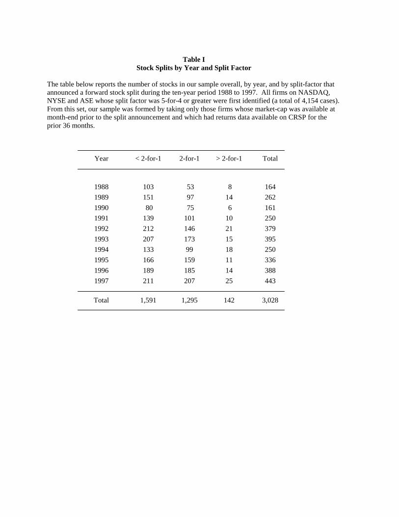
Table I

Stock Splits by Year and Split Factor

The table below reports the number of stocks in our sample overall, by year, and by split-factor that announced a forward stock split during the ten-year period 1988 to 1997. All firms on NASDAQ, NYSE and ASE whose split factor was 5-for-4 or greater were first identified (a total of 4,154 cases). From this set, our sample was formed by taking only those firms whose market-cap was available at month-end prior to the split announcement and which had returns data available on CRSP for the prior 36 months.

Year < 2-for-1 2-for-1 > 2-for-1 Total

1988 103 53 8 164 1989 151 97 14 262 1990 80 75 6 161 1991 139 101 10 250 1992 212 146 21 379 1993 207 173 15 395 1994 133 99 18 250 1995 166 159 11 336 1996 189 185 14 388 1997 211 207 25 443

Total 1,591 1,295 142 3,028

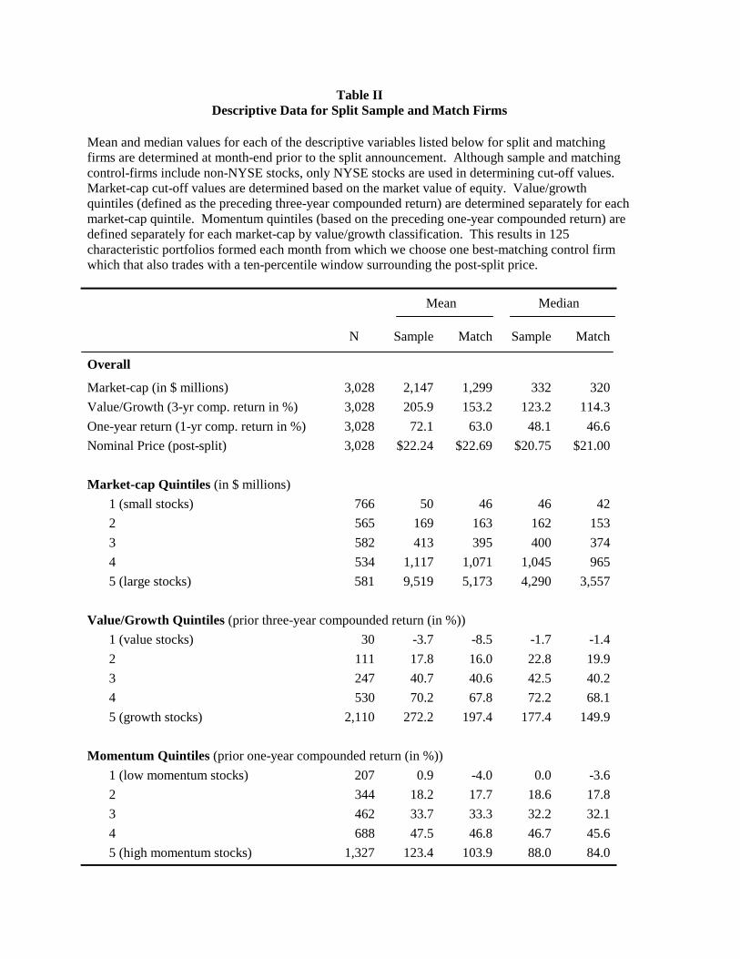
Table II Descriptive Data for Split Sample and Match Firms

Mean and median values for each of the descriptive variables listed below for split and matching firms are determined at month-end prior to the split announcement. Although sample and matching control-firms include non-NYSE stocks, only NYSE stocks are used in determining cut-off values. Market-cap cut-off values are determined based on the market value of equity. Value/growth quintiles (defined as the preceding three-year compounded return) are determined separately for each market-cap quintile. Momentum quintiles (based on the preceding one-year compounded return) are defined separately for each market-cap by value/growth classification. This results in 125 characteristic portfolios formed each month from which we choose one best-matching control firm which that also trades with a ten-percentile window surrounding the post-split price.

Mean Median N Sample Match Sample Match Overall

Market-cap (in $ millions) 3,028 2,147 1,299 332 320 Value/Growth (3-yr comp. return in %) 3,028 205.9 153.2 123.2 114.3 One-year return (1-yr comp. return in %) 3,028 72.1 63.0 48.1 46.6 Nominal Price (post-split) 3,028 $22.24 $22.69 $20.75 $21.00 Market-cap Quintiles (in $ millions)

1 (small stocks) 766 50 46 46 42 2 565 169 163 162 153 3 582 413 395 400 374 4 534 1,117 1,071 1,045 965 5 (large stocks) 581 9,519 5,173 4,290 3,557

Value/Growth Quintiles (prior three-year compounded return (in %))

1 (value stocks) 30 -3.7 -8.5 -1.7 -1.4 2 111 17.8 16.0 22.8 19.9 3 247 40.7 40.6 42.5 40.2 4 530 70.2 67.8 72.2 68.1 5 (growth stocks) 2,110 272.2 197.4 177.4 149.9

Momentum Quintiles (prior one-year compounded return (in %))

1 (low momentum stocks) 207 0.9 -4.0 0.0 -3.6 2 344 18.2 17.7 18.6 17.8 3 462 33.7 33.3 32.2 32.1 4 688 47.5 46.8 46.7 45.6 5 (high momentum stocks) 1,327 123.4 103.9 88.0 84.0

Table III One-year post-split returns (in %) for sample and matching control firms

This table reports compounded returns for the period starting two trading days after a split announcement and ending 250 trading days later for sample firms and matching control firms. Returns are calculated three different ways. First, we report overall returns for all firms in our sample. The second approach, real-time truncation, is based on a strategy of prematurely liquidating the investment in both the sample and match firms on the first day in which the difference in compounded return between that sample firm and its match exceeds 100%. In the third approach, we symmetrically winsorize the sample, ex-post, at the 1% and 99% levels. Numbers in parentheses represent significance levels for t-tests of the means and a Wilcoxon signed-rank test for medians.

Overall Real-Time Truncation Winsorized Mean Median Mean Median Mean Median

Split 23.29 16.18 22.52 17.21 22.44 16.18 Match 14.29 11.01 14.26 10.66 13.87 11.01

Paired-Difference 9.00 6.31 8.26 6.88 8.52 6.31

(t=7.93; p<0.0001)

(p<0.0001) (t=8.23; p<0.0001)

(p<0.0001) (t=8.37; p<0.0001)

(p<0.0001)

Table IV One-Year Post-Split Abnormal Returns by Year, Exchange Listing and Split Factor

This table reports paired differences in compounded returns between split-announcing and matching control firms by year, exchange, and split factor. Returns are for the period starting two trading days after the split announcement date and ending 250 trading days after the announcement. Numbers in parentheses represent significance levels for t-tests of the means and a Wilcoxon signed-rank test for medians.

N

Mean

Median By year of split

1988-89 426 6.82 6.49

(t=2.70; p<0.0072) (p<0.0045)

1990-91 411 10.84 6.86 (t=3.16; p<0.0017) (p<0.0026)

1992-93 774 7.48 4.15 (t=3.61; p<0.0003) (p<0.0003)

1994-95 586 11.02 6.44 (t=3.55; p<0.0004) (p<0.0015)

1996-97 831 9.19 7.18 (t=4.58; p<0.0001) (p<0.0001)

By Exchange

NYSE 1,148 7.63 5.58

(t=5.05; p<0.0001) (p<0.0001)

AMEX 285 7.36 5.89 (t=2.02; p<0.0440) (p<0.0344)

NASDAQ 1,595 10.27 7.18 (t=5.90; p<0.0001) (p<0.0001)

By Split Factor

< 2-for-1 1,591 10.4 6.64

(t=6.58; p<0.0001) (p<0.0001)

2-for-1 1,295 6.75 5.81 (t=3.94; p<0.0001) (p<0.0001)

> 2-for-1 142 13.74 6.21 (t=2.66; p<0.0086) (p<0.0001)

Table V One-Year Post-Split Abnormal Returns by Market-cap, Value/growth and Momentum

This table reports compounded abnormal returns for portfolios formed on the basis of firm characteristics for a one-year holding period starting two trading days after the split announcement date and ending 250 trading days. Market-cap cut-off values are determined based on the market value of equity of only NYSE stocks. Value/growth quintiles (defined as the preceding three-year compounded return) are determined separately for each NYSE size category. Momentum quintiles (based on the preceding one-year compounded return) are defined separately for each market-cap by value/growth category. Numbers in parentheses represent significance levels for t-tests of the means and a Wilcoxon signed-rank test for medians.

N Mean Median

Market-cap Quintiles (in $ millions)

1 (small stocks) 766 12.37 9.31 (t=4.53; p<0.0001) (p<0.0001)

2 565 11.03 6.42 (t=4.03; p<0.0001) (p<0.0003)

3 582 11.94 11.33 (t=4.67; p<0.0001) (p<0.0001)

4 534 3.78 2.65 (t=1.66; p<0.0982) (p<0.2181)

5 (large stocks) 581 4.42 4.17 (t=2.25; p<0.0247) (p<0.0317)

Value/Growth Quintiles (prior three-year compounded return (in %))

1 (value stocks) 30 37.47 10.25 (t=1.62; p<0.1152) (p<0.0984)

2 111 11.00 6.15 (t=2.49; p<0.0141) (p<0.0290)

3 247 2.13 0.20 (t=0.73; p<0.4668) (p<0.3467)

4 530 6.83 6.37 (t=3.09; p<0.0021) (p<0.0001)

5 (growth stocks) 2,110 9.84 6.73 (t=6.86; p<0.0001) (p<0.0001)

Momentum Quintiles (prior one-year compounded return (in %))

1 (low momentum stocks) 207 6.11 8.67 (t=1.35; p<0.1788) (p<0.0336)

2 344 6.96 4.96 (t=2.90; p<0.0040) (p<0.0098)

3 462 6.66 5.68 (t=2.72; p<0.0069) (p<0.0071)

4 688 10.28 7.12 (t=5.30; p<0.0001) (p<0.0001)

5 (high momentum stocks) 1,327 10.12 5.89 (t=5.02; p<0.0001) (p<0.0001)

Table VI Analyst Following for Split and Match-Control Firms

This table reports mean and median analyst following for split and matching control firms from ten days prior to split announcement to three days before the first annual earnings announcement. In cases where the first annual earnings announcement is within six months of the split announcement date, the next fiscal year is used in the analysis. Analyst following for both sample and control firms is measured in event time relative to their respective earnings announcement dates and is measured as the number of individual analysts submitting annual earnings forecasts to I/B/E/S for that fiscal year.

After the Split Announcement Before the Earnings Announcement

10 Days Before Split

10 days

1 month

2 months

3 months

3 months

2 months

1 month

3 days

Number of Analysts following split firms

Mean 12.68 13.06 13.24 13.61 14.05 15.52 15.89 16.16 16.36

Median 9.00 10.00 10.00 10.00 11.00 12.00 12.50 13.00 13.00

Number of Analysts following match firms

Mean 13.08 13.48 13.69 14.04 14.40 15.94 16.28 16.54 16.74

Median 10.00 10.00 11.00 11.00 11.00 12.00 12.00 13.00 13.00

Table VII Change in Earnings Yield for Split and Match-Control Firms

and the S&P Industrial Index

This table reports the growth in earnings yield for 948 split announcing firms and their respective matches from the year before to the year following the split. Actual earnings (adjusted for unusual items) are obtained from I/B/E/S. The difference in earnings per share is computed as the annual earnings reported after the split announcement less previous year's earnings, scaled by month-end stock price preceding the split announcement. If the annual earnings are reported within 125 trading days of the split date, we use reported earnings at the next fiscal year-end. EPS differences for match firms are computed similarly by aligning fiscal years as closely as possible with their split-announcing counterparts. For comparison, we also report changes in earnings yield for the S&P industrial index at the same point in time. Numbers in parentheses represent significance levels for t-tests of the means and a Wilcoxon signed-rank test for medians.

Mean

Median %

positive Split Sample 1.18 0.95 84.7 (t=14.55; p<0.0001) (p<0.0001) Match Firms 0.92 0.91 72.9 (t=6.65; p<0.0001) (p<0.0001) S&P Industrial Index 0.38 0.48 --- Difference in Earnings Yield Growth (Split – Match Firms)

0.26

0.14

52.7

(t=1.66; p<0.0968) (p<0.0206) Difference in Growth (Split Firms - S&P Index)

0.79

0.59

71.7

(t=9.19; p<0.0001) (p<0.0001)

Table VIII Revisions in Earnings Expectations Subsequent to Stock Split Announcements

This table reports the evolution of earnings expectations for a subset of 948 split announcements with forecast data available on I/B/E/S. The following measure is computed for both the sample firms and their matching firms:

∑∑==

= n

i ti

n

i titI PAPFFPA1 ,1 ,, )/(/)/(

where FPAI,t is the forecasted EPS expressed as a percentage of actual EPS for group I (I=sample, match) as of time t. (F/P)i,t is the mean I/B/E/S forecast for firm i as of time t scaled by its stock price at month-end prior to the split announcement and (A/P)i,t is the actual earnings for the year after the split, scaled by the same (split-adjusted) stock price. If the first post-split earnings announcement is within 125 days of the split announcement, we jump to the next annual earnings cycle. The difference in FPA is computed as FPAS,t - FPAM,t where S is the set of sample firms and M the set of match firms. P-values which examine the significance of each difference are reported in parentheses. Significance is estimated using a randomization procedure over 10,000 trials. The p-values show the fraction of random cases generated under the null-hypothesis with differences less than the hypothesized value.

After the Split Announcement Before the Earnings Announcement

10 Days Before Split

10 days

1 month

2 months

3 months

3 Months

2 Months

1 Month

3 Days

Overall FPA for Split Firms (in %) 97.83 98.63 98.79 99.42 99.70 99.85 99.71 99.46 99.31 FPA for Match Firms (in %) 105.50 105.71 105.62 105.43 104.93 102.88 102.67 102.11 101.99 Difference in FPA Overall (Sample minus Match) -7.67 -7.08 -6.82 -6.01 -5.23 -3.03 -2.96 -2.65 -2.68

(.0002) (<.0001) (<.0001) (<.0001) (.0012) (.0106) (.0077) (.0128) (.0088)

Difference in FPA for Large-Cap (Q5) -5.86 -5.34 -5.24 -4.55 -4.29 -1.25 -1.32 -1.20 -1.16 (.0605) (.0762) (.0832) (.1094) (.1235) (.2785) (.2579) (.2678) (.2839) Difference in FPA for Small & Med-cap (Q1 to Q4) -8.32 -7.71 -7.39 -6.54 -5.57 -3.71 -3.57 -3.20 -3.24

(<.0001) (.0001) (.0003) (.0001) (.0020) (.0100) (.0104) (.0124) (.0098) Difference in FPA for High Growth (Q5) -9.59 -9.07 -9.81 -7.82 -6.82 -4.10 -3.65 -3.15 -3.10 (.0001) (.0005) (<.0001) (.0005) (.0010) (.0123) (.0167) (.0279) (.0248) Difference in FPA for Value and medium (Q1 to Q4) -5.06 -4.38 -4.11 -3.55 -3.06 -1.59 -2.01 -1.98 -2.11

(.0475) (.0717) (.0723) (.1032) (.1358) (.1987) (.1160) (.1076) (.0928) Difference in FPA for High momentum (Q5) -9.96 -8.64 -8.38 -7.17 -5.95 -3.73 -3.86 -3.17 -3.14 (.0021) (.0072) (.0069) (.0137) (.0357) (.0596) (.0455) (.069) (.0693) Difference in FPA for Low and medium (Q1 to Q4) -6.19 -6.07 -5.81 -5.25 -4.74 -2.58 -2.37 -2.31 -2.37 (.0016) (.0014) (.0019) (.0034) (.0056) (.0350) (.0377) (.0385) (.0296)

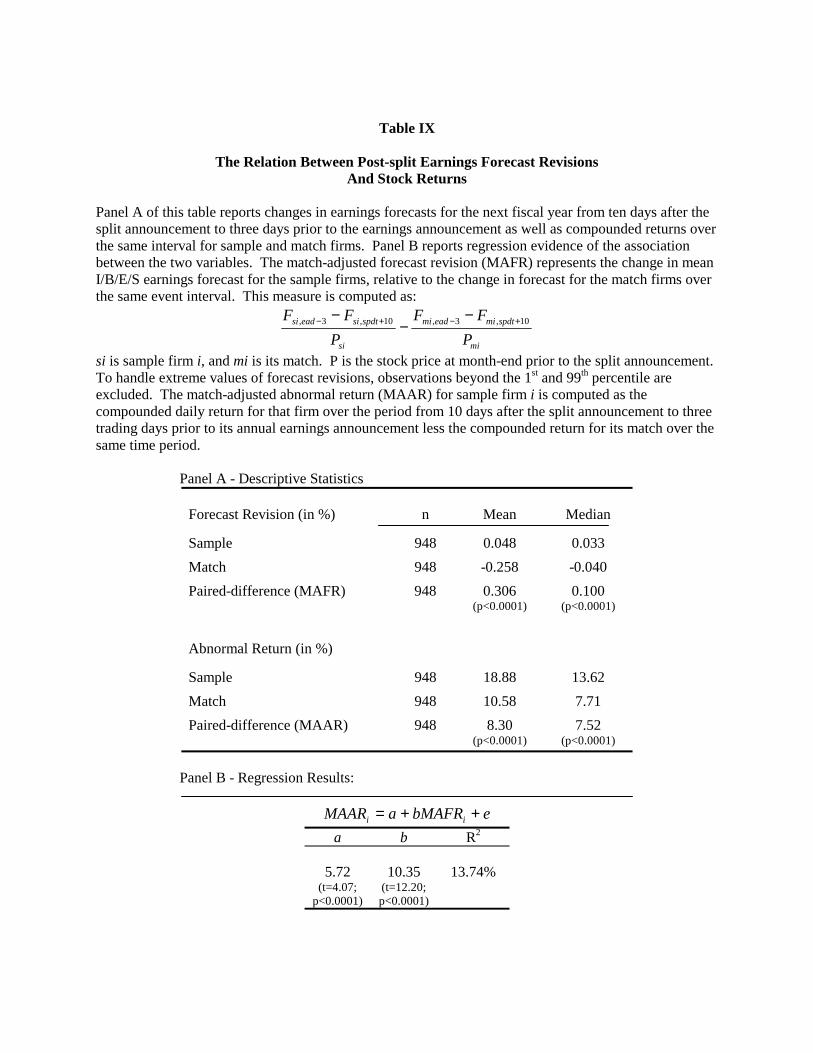
Table IX

The Relation Between Post-split Earnings Forecast Revisions And Stock Returns

Panel A of this table reports changes in earnings forecasts for the next fiscal year from ten days after the split announcement to three days prior to the earnings announcement as well as compounded returns over the same interval for sample and match firms. Panel B reports regression evidence of the association between the two variables. The match-adjusted forecast revision (MAFR) represents the change in mean I/B/E/S earnings forecast for the sample firms, relative to the change in forecast for the match firms over the same event interval. This measure is computed as:

mi

spdtmieadmi

si

spdtsieadsi

PFF

PFF 10,3,10,3, +−+− −

−−

si is sample firm i, and mi is its match. P is the stock price at month-end prior to the split announcement. To handle extreme values of forecast revisions, observations beyond the 1st and 99th percentile are excluded. The match-adjusted abnormal return (MAAR) for sample firm i is computed as the compounded daily return for that firm over the period from 10 days after the split announcement to three trading days prior to its annual earnings announcement less the compounded return for its match over the same time period.

Panel A - Descriptive Statistics Forecast Revision (in %) n Mean Median

Sample 948 0.048 0.033 Match 948 -0.258 -0.040 Paired-difference (MAFR) 948 0.306 0.100 (p<0.0001) (p<0.0001)

Abnormal Return (in %)

Sample 948 18.88 13.62 Match 948 10.58 7.71 Paired-difference (MAAR) 948 8.30 7.52 (p<0.0001) (p<0.0001)

Panel B - Regression Results:

ebMAFRaMAAR ii ++=

a b R2

5.72 10.35 13.74% (t=4.07;

p<0.0001) (t=12.20; p<0.0001)

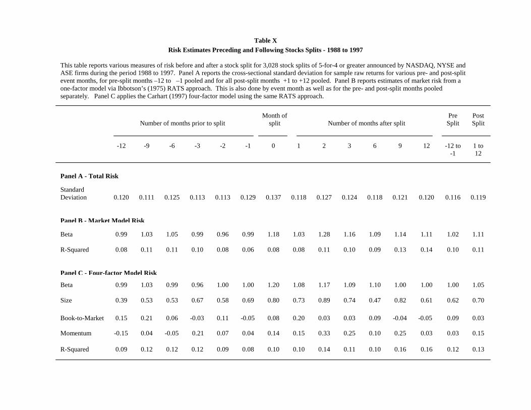
Table X Risk Estimates Preceding and Following Stocks Splits - 1988 to 1997

This table reports various measures of risk before and after a stock split for 3,028 stock splits of 5-for-4 or greater announced by NASDAQ, NYSE and ASE firms during the period 1988 to 1997. Panel A reports the cross-sectional standard deviation for sample raw returns for various pre- and post-split event months, for pre-split months –12 to –1 pooled and for all post-split months +1 to +12 pooled. Panel B reports estimates of market risk from a one-factor model via Ibbotson’s (1975) RATS approach. This is also done by event month as well as for the pre- and post-split months pooled separately. Panel C applies the Carhart (1997) four-factor model using the same RATS approach.

Number of months prior to split

Month of

split

Number of months after split

Pre

Split

Post Split

-12

-9

-6

-3

-2

-1

0

1

2

3

6

9

12

-12 to

-1

1 to 12

Panel A - Total Risk

Standard Deviation

0.120

0.111

0.125

0.113

0.113

0.129

0.137

0.118

0.127

0.124

0.118

0.121

0.120

0.116

0.119

Panel B - Market Model Risk

Beta

0.99

1.03

1.05

0.99

0.96

0.99

1.18

1.03

1.28

1.16

1.09

1.14

1.11

1.02

1.11

R-Squared

0.08

0.11

0.11

0.10

0.08

0.06

0.08

0.08

0.11

0.10

0.09

0.13

0.14

0.10

0.11

Panel C - Four-factor Model Risk

Beta 0.99 1.03 0.99 0.96 1.00 1.00 1.20 1.08 1.17 1.09 1.10 1.00 1.00 1.00 1.05

Size 0.39 0.53 0.53 0.67 0.58 0.69 0.80 0.73 0.89 0.74 0.47 0.82 0.61 0.62 0.70 Book-to-Market

0.15

0.21

0.06

-0.03

0.11

-0.05

0.08

0.20

0.03

0.03

0.09

-0.04

-0.05

0.09

0.03

Momentum -0.15 0.04 -0.05 0.21 0.07 0.04 0.14 0.15 0.33 0.25 0.10 0.25 0.03 0.03 0.15 R-Squared 0.09 0.12 0.12 0.12 0.09 0.08 0.10 0.10 0.14 0.11 0.10 0.16 0.16 0.12 0.13

Table XI Post-Split Abnormal Returns (in %) for Non-dividend Paying Firms

Panel A reports compounded returns for the period starting two trading days after the split announcement and ending 250 trading days later for 889 sample firms which did not pay a dividend both in the year before and year of the split. Returns are calculated using the same methods detailed in Table III. Panel B reports return differences for various sub-samples. Numbers in parentheses represent significance levels for t-tests of the means and a Wilcoxon signed-rank test for medians. Panel A: Abnormal stock returns for non-dividend paying split firms

Overall Real-Time Truncation Winsorized

Mean Median Mean Median Mean Median

Split 24.45 12.78 22.84 15.83 23.24 12.78 Match 12.68 6.15 12.52 5.41 12.11 6.15

Difference 11.77 7.45 10.32 9.71 10.87 7.45 (t=4.34; p<0.0001) (p<0.0003) (t=4.62; p<0.0001) (p<0.0001) (t=4.55; p<0.0001) (p<0.0003)

Panel B: Abnormal stock returns by group

N Mean Significance Median Significance By year of split

1988-92 301 14.00 t=3.03;p<0.0026 10.43 p<0.0034

1993-97 588 10.63 t=3.17; p<0.0016 5.48 p<0.0188

By Exchange NYSE & AMEX 293 9.81 t=2.28; p<0.0234 8.29 p<0.0158

NASDAQ 596 12.74 t=3.69; p<0.0002 6.66 p<0.0057

By Split Factor

< 2-for-1 463 15.73 t=4.06; p<0.0001 9.85 p<0.0003

2-for-1 or greater 426 7.48 t=1.97; p<0.0490 4.58 p<0.1506

By Market-cap Quintiles

1 and 2 456 12.76 t=3.00; p<0.0028 7.62 p<0.0197

3, 4 and 5 433 10.73 t=3.23; p<0.0013 6.58 p<0.0049

By Value/Growth Quintiles

1 and 2 22 51.20 t=1.61; p<0.1205 17.62 p<0.1342

3, 4 and 5 867 10.77 t=4.05;p<0.0001 7.12 p<0.0007

By Momentum Quintiles

1 and 2 126 11.86 t=2.01; p<0.0466 16.22 p<0.0087

3, 4 and 5 763 11.76 t=3.91; p<0.0001 6.31 p<0.0044

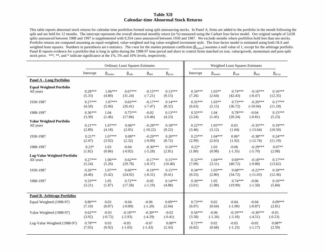
Table XII Calendar-time Abnormal Stock Returns

This table reports abnormal stock returns for calendar-time portfolios formed using split announcing stocks. In Panel A, firms are added to the portfolio in the month following the split and are held for 12 months. The intercept represents the overall abnormal monthly return (in %) measured using the Carhart four-factor model. Our original sample of 3,028 splits announced between 1988 and 1997 is supplemented with 9,354 cases announced between 1930 and 1987. We exclude months where portfolios hold less than ten stocks. Portfolio returns are computed assuming an equal-weighted, value-weighted and log value-weighted investment style. The four-factor model is estimated using both OLS and weighted least squares. Numbers in parenthesis are t-statistics. The t-test for the market premium coefficient (βmarket) assumes a null value of 1, except for the arbitrage portfolio. Panel B reports evidence for a portfolio that is long in splits during the 1988-97 time period and short in control firms matched on size, value/growth, momentum and post-split stock price. ***, **, and * indicate significance at the 1%, 5% and 10% levels, respectively.

Ordinary Least Squares Estimates Weighted Least Squares Estimates

Intercept βmarket βsmb βhml βpr1yr Intercept βmarket βsmb βhml βpr1yr

Panel A - Long Portfolios

Equal Weighted Portfolio All years 0.28*** 1.06*** 0.67*** -0.15*** 0.13*** 0.34*** 1.03** 0.74*** -0.16*** 0.16*** (5.33) (4.80) (31.24) (-7.21) (9.15) (7.26) (2.64) (42.43) (-8.47) (12.35)

1930-1987 0.27*** 1.07*** 0.65*** -0.17*** 0.14*** 0.35*** 1.03** 0.73*** -0.20*** 0.17*** (4.50) (5.06) (26.41) (-7.47) (8.32) (6.63) (2.15) (36.72) (-10.04) (11.18)

1988-1997 0.36*** 1.04 0.75*** -0.02 0.13*** 0.33*** 1.04 0.78*** -0.04 0.15*** (3.39) (1.46) (17.84) (-0.46) (4.23) (3.24) (1.45) (20.24) (-0.81) (5.23) Value Weighted Portfolio All years 0.21*** 1.07*** 0.06** -0.28*** 0.18*** 0.22*** 1.05*** 0.03 -0.35*** 0.19*** (2.89) (4.18) (2.05) (-10.22) (9.22) (3.46) (3.12) (1.04) (-13.64) (10.50)

1930-1987 0.21** 1.07*** 0.08** -0.29*** 0.20*** 0.23*** 1.04*** 0.06* -0.38*** 0.24*** (2.47) (3.92) (2.32) (-9.09) (8.72) (2.99) (2.63) (1.92) (-12.74) (11.19)

1988-1997 0.23* 1.03 -0.04 -0.30*** 0.10*** 0.22* 1.03 -0.06 -0.29*** 0.07** (1.82) (0.86) (-0.82) (-5.28) (2.81) (1.80) (0.98) (-1.35) (-5.70) (2.08) Log-Value Weighted Portfolio All years 0.27*** 1.06*** 0.62*** -0.17*** 0.15*** 0.32*** 1.04*** 0.69*** -0.18*** 0.17*** (5.24) (5.26) (29.78) (-8.37) (10.40) (7.09) (3.31) (40.72) (-9.88) (13.62)

1930-1987 0.26*** 1.07*** 0.60*** -0.19*** 0.15*** 0.34*** 1.03*** 0.68*** -0.22*** 0.18*** (4.46) (5.42) (24.92) (-8.31) (9.41) (6.55) (2.80) (34.72) (-11.03) (12.36)

1988-1997 0.33*** 1.05 0.72*** -0.05 0.14*** 0.30*** 1.05 0.74*** -0.06 0.16*** (3.21) (1.87) (17.58) (-1.19) (4.88) (3.01) (1.88) (19.90) (-1.58) (5.84)

Panel B- Arbitrage Portfolios

Equal Weighted (1988-97) 0.80*** 0.03 -0.04 -0.06 0.09*** 0.73*** 0.02 -0.04 -0.04 0.09*** (7.10) (0.87) (-0.89) (-1.20) (2.64) (6.97) (0.64) (-1.00) (-0.87) (2.81)

Value Weighted (1988-97) 0.62*** -0.03 -0.18*** -0.30*** -0.02 0.56*** -0.06 -0.19*** -0.30*** -0.01 (3.92) (-0.72) (-2.93) (-4.29) (-0.41) (3.58) (-1.26) (-3.18) (-4.51) (-0.23)

Log-Value Weighted (1988-97) 0.78*** 0.03 -0.05 -0.07 0.08** 0.72*** 0.02 -0.05 -0.05 0.08** (7.03) (0.92) (-1.05) (-1.43) (2.43) (6.82) (0.68) (-1.23) (-1.17) (2.59)

Figure 1

Frequency Distribution of Earnings Growth for Split-Announcing and Match Firms

This graph plots the distribution of changes in earnings yield for both split firms and matching control- firms around the time of a stock split. For each sample firm, the change in earnings is computed as the difference between year-end operating earnings reported after the split announcement compared to the same number prior to the split. If the length of time between the split announcement and the next annual earnings release is less than six-months, we discard this number and use earnings in the following year. These changes in earnings are normalized by price in the month following the split announcement. I/B/E/S was our source for actual operating earnings adjusted for unusual items.

0%

5%

10%

15%

20%

25%

30%

-0.1

-0.0

8

-0.0

7

-0.0

5

-0.0

4

-0.0

2

-0.0

1

0.0

0

0.0

2

0.0

3

0.0

5

0.0

6

0.0

8

0.0

9

Split

Match

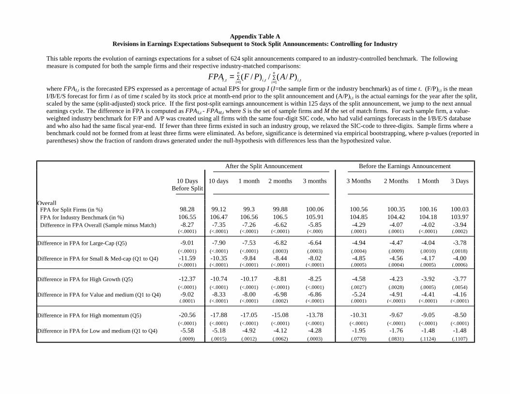
Appendix Table A Revisions in Earnings Expectations Subsequent to Stock Split Announcements: Controlling for Industry

This table reports the evolution of earnings expectations for a subset of 624 split announcements compared to an industry-controlled benchmark. The following measure is computed for both the sample firms and their respective industry-matched comparisons:

∑∑==

= n

i ti

n

i titI PAPFFPA1 ,1 ,, )/(/)/(

where FPAI,t is the forecasted EPS expressed as a percentage of actual EPS for group I (I=the sample firm or the industry benchmark) as of time t. (F/P)i,t is the mean I/B/E/S forecast for firm i as of time t scaled by its stock price at month-end prior to the split announcement and (A/P)i,t is the actual earnings for the year after the split, scaled by the same (split-adjusted) stock price. If the first post-split earnings announcement is within 125 days of the split announcement, we jump to the next annual earnings cycle. The difference in FPA is computed as FPAS,t - FPAM,t where S is the set of sample firms and M the set of match firms. For each sample firm, a value-weighted industry benchmark for F/P and A/P was created using all firms with the same four-digit SIC code, who had valid earnings forecasts in the I/B/E/S database and who also had the same fiscal year-end. If fewer than three firms existed in such an industry group, we relaxed the SIC-code to three-digits. Sample firms where a benchmark could not be formed from at least three firms were eliminated. As before, significance is determined via empirical bootstrapping, where p-values (reported in parentheses) show the fraction of random draws generated under the null-hypothesis with differences less than the hypothesized value.

After the Split Announcement Before the Earnings Announcement

10 Days Before Split

10 days

1 month

2 months

3 months

3 Months

2 Months

1 Month

3 Days

Overall FPA for Split Firms (in %) 98.28 99.12 99.3 99.88 100.06 100.56 100.35 100.16 100.03 FPA for Industry Benchmark (in %) 106.55 106.47 106.56 106.5 105.91 104.85 104.42 104.18 103.97 Difference in FPA Overall (Sample minus Match) -8.27 -7.35 -7.26 -6.62 -5.85 -4.29 -4.07 -4.02 -3.94

(<.0001) (<.0001) (<.0001) (<.0001) (<.000) (.0001) (.0001) (<.0001) (.0002)

Difference in FPA for Large-Cap (Q5) -9.01 -7.90 -7.53 -6.82 -6.64 -4.94 -4.47 -4.04 -3.78 (<.0001) (<.0001) (<.0001) (.0003) (.0003) (.0004) (.0009) (.0010) (.0018) Difference in FPA for Small & Med-cap (Q1 to Q4) -11.59 -10.35 -9.84 -8.44 -8.02 -4.85 -4.56 -4.17 -4.00

(<.0001) (<.0001) (<.0001) (<.0001) (<.0001) (.0005) (.0004) (.0005) (.0006) Difference in FPA for High Growth (Q5) -12.37 -10.74 -10.17 -8.81 -8.25 -4.58 -4.23 -3.92 -3.77 (<.0001) (<.0001) (<.0001) (<.0001) (<.0001) (.0027) (.0028) (.0005) (.0054) Difference in FPA for Value and medium (Q1 to Q4) -9.02 -8.33 -8.00 -6.98 -6.86 -5.24 -4.91 -4.41 -4.16

(.0001) (<.0001) (<.0001) (.0002) (<.0001) (.0001) (<.0001) (<.0001) (<.0001) Difference in FPA for High momentum (Q5) -20.56 -17.88 -17.05 -15.08 -13.78 -10.31 -9.67 -9.05 -8.50 (<.0001) (<.0001) (<.0001) (<.0001) (<.0001) (<.0001) (<.0001) (<.0001) (<.0001) Difference in FPA for Low and medium (Q1 to Q4) -5.58 -5.18 -4.92 -4.12 -4.28 -1.95 -1.76 -1.48 -1.48 (.0009) (.0015) (.0012) (.0062) (.0003) (.0770) (.0831) (.1124) (.1107)

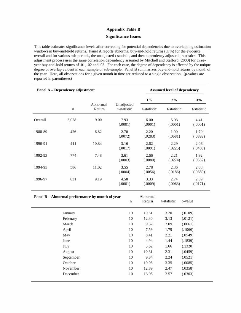
Appendix Table B Significance Issues

This table estimates significance levels after correcting for potential dependencies due to overlapping estimation windows in buy-and-hold returns. Panel A reports abnormal buy-and-hold returns (in %) for the evidence overall and for various sub-periods, the unadjusted t-statistic, and then dependency adjusted t-statistics. This adjustment process uses the same correlation dependency assumed by Mitchell and Stafford (2000) for three-year buy-and-hold returns of .01, .02 and .03. For each case, the degree of dependency is affected by the unique degree of overlap evident in each sample or sub-sample. Panel B summarizes buy-and-hold returns by month of the year. Here, all observations for a given month in time are reduced to a single observation. (p-values are reported in parentheses)

Panel A – Dependency adjustment Assumed level of dependency

1% 2% 3% Abnormal Unadjusted n Return t-statistic t-statistic t-statistic t-statistic

Overall 3,028 9.00 7.93 6.00 5.03 4.41 (.0001) (.0001) (.0001) (.0001)

1988-89 426 6.82 2.70 2.20 1.90 1.70 (.0072) (.0283) (.0581) (.0899)

1990-91 411 10.84 3.16 2.62 2.29 2.06 (.0017) (.0091) (.0225) (.0400)

1992-93 774 7.48 3.61 2.66 2.21 1.92 (.0003) (.0080) (.0274) (.0552)

1994-95 586 11.02 3.55 2.78 2.36 2.08 (.0004) (.0056) (.0186) (.0380)

1996-97 831 9.19 4.58 3.33 2.74 2.39 (.0001) (.0009) (.0063) (.0171)

Panel B – Abnormal performance by month of year n

Abnormal Return

t-statistic

p-value

January 10 10.51 3.20 (.0109) February 10 12.30 3.13 (.0121) March 10 9.32 2.09 (.0661) April 10 7.59 1.79 (.1066) May 10 8.41 2.21 (.0549) June 10 4.94 1.44 (.1839) July 10 5.62 1.66 (.1320) August 10 10.31 2.31 (.0459) September 10 9.84 2.24 (.0521) October 10 19.03 3.35 (.0085) November 10 12.89 2.47 (.0358) December 10 13.95 2.57 (.0303)