underlying dynamics of typical fluctuations of an emerging market price index: the heston model from...

ARTICLE IN PRESS

Physica A 361 (2006) 272–288

0378-4371/$ -

doi:10.1016/j

�CorrespoE-mail ad

www.elsevier.com/locate/physa

Underlying dynamics of typical fluctuations of anemerging market price index: The Heston model

from minutes to months

Renato Vicentea, Charles M. de Toledob,Vitor B.P. Leitec, Nestor Catichad,�

aEscola de Artes, Ciencias e Humanidades, Universidade de Sao Paulo, Parque Ecologico do Tiete,

03828-020, Sao Paulo - SP, BrazilbBOVESPA - Sao Paulo Stock Exchange, R. XV de Novembro, 275, 01013-001 Sao Paulo - SP, BrazilcDep. de Fısica, IBILCE, Universidade Estadual Paulista, 15054-000 Sao Jose do Rio Preto - SP, Brazil

dDep. de Fısica Geral, Instituto de Fısica, Universidade de Sao Paulo, Caixa Postal 66318,

05315-970 Sao Paulo - SP, Brazil

Received 11 February 2004; received in revised form 16 May 2005

Available online 11 August 2005

Abstract

We investigate the Heston model with stochastic volatility and exponential tails as a model

for the typical price fluctuations of the Brazilian Sao Paulo Stock Exchange Index

(IBOVESPA). Raw prices are first corrected for inflation and a period spanning 15 years

characterized by memoryless returns is chosen for the analysis. Model parameters are

estimated by observing volatility scaling and correlation properties. We show that the Heston

model with at least two time scales for the volatility mean reverting dynamics satisfactorily

describes price fluctuations ranging from time scales larger than 20min to 160 days. At time

scales shorter than 20min we observe autocorrelated returns and power law tails incompatible

with the Heston model. Despite major regulatory changes, hyperinflation and currency crises

experienced by the Brazilian market in the period studied, the general success of the

description provided may be regarded as an evidence for a general underlying dynamics of

price fluctuations at intermediate mesoeconomic time scales well approximated by the Heston

model. We also notice that the connection between the Heston model and Ehrenfest urn

see front matter r 2005 Elsevier B.V. All rights reserved.

.physa.2005.06.095

nding author. Tel.: +5511 30916798.

dress: [email protected] (R. Vicente).

www.elsevier.com/locate/physa

ARTICLE IN PRESS

R. Vicente et al. / Physica A 361 (2006) 272–288 273

models could be exploited for bringing new insights into the microeconomic market

mechanics.

r 2005 Elsevier B.V. All rights reserved.

Keywords: Econophysics; Stochastic volatility; Heston model; High-frequency finance

1. Introduction

In the last decades the quantitative finance community has devoted muchattention to the modeling of asset returns having as a major drive the improvementof pricing techniques [1] by employing stochastic volatility models ameanable toanalytical treatment such as Hull–White [2], Stein–Stein [3] and Heston [4] models.

Despite differences in methods and emphasis, the cross fecundation betweenEconomics and Physics, which dates back to the early 19th century (see Refs. [5,6]),has intensified recently [7]. Following the statistical physics approach, substantialeffort has been made to find microeconomic models capable of reproducing a numberof recurrent features of financial time series such as: returns aggregation (probabilitydistributions at any time scale) [8,9], volatility clustering [11], leverage effect(correlation between returns and volatilities) [12,13], conditional correlations [14,15]and fat tails at very short time scales [7]. A central feature of economical phenomena isthe prevalence of intertwined dynamics at several time scales. In very general terms,one could divide the market dynamics onto three broad classes: the microeconomicdynamics at the time scales of books of orders and price formation, the mesoeconomicdynamics at the scales of oscillations in formed prices due to local supply and demandand the macroeconomic dynamics at the scales of aggregated economy trends.

The literature on empirical finance have emphasized the multifractal scaling [16]and the power law tails of price fluctuations. However, it has been shown [17] thatvery large data sets are required in order to distinguish between a multifractal andpower law tailed process and a stochastic volatility model. In this paper we,therefore, deal with the mesoeconomic dynamics as it would be described by theHeston model with stochastic volatility and exponential tails.

Recently, a semi-analytical solution for the Fokker–Planck equation describing thedistribution of log-returns in the Heston model has been proposed [8]. The authorswere able to show a satisfactory agreement between return distributions of a numberof developed market stock indices and the model for time scales spanning a wideinterval ranging from 1 to 100days. More recently, the same model has also beenemployed to describe single stocks intraday fluctuations with relative success [10].

In this paper we show evidence that the Heston model is also capable of describingthe fluctuation dynamics of an emerging market price index, the Brazilian Sao PauloStock Exchange Index (IBOVESPA). We employ for the analysis 37 years of datasince IBOVESPA inception in January, 1968 and approximately 4 years of intradaydata as well. In this period the Brazilian economy has experienced periods ofpolitical and economical unrest, of hyperinflation, of currency crises and of majorregulatory changes. These distinctive characteristics make the IBOVESPA an

ARTICLE IN PRESS

R. Vicente et al. / Physica A 361 (2006) 272–288274

interesting ground for general modelling and data analysis and for testing the limitsof description of the Heston model.

This paper is organized as follows. The next section surveys the Heston model, itssemi-analytical solution and its connection to Ehrenfest urn models. Section 3discusses the pre-processing necessary for isolating the fluctuations to be describedby the Heston model from exogenous effects. Section 4 describes the data analysis atlow (from daily fluctuations) and high (intraday fluctuations) frequencies.Conclusions and further directions are presented in Section 5.

2. Heston model

2.1. Semi-analytical solution

The Heston model describes the dynamics of stock prices St as a geometricBrownian motion with volatility given by a Cox–Ingersoll–Ross (or Feller) mean-reverting dynamics. In the Ito differential form the model reads

dSt ¼ St mt dtþ St

ffiffiffiffivt

pdW 0ðtÞ ,

dvt ¼ � g½vt � y�dtþ kffiffiffiffivt

pdW 1ðtÞ , ð1Þ

where vt represents the square of the volatility and dW j are Wiener processes with

hdW jðtÞi ¼ 0 ,

hdW jðtÞdW kðt0Þi ¼ dðt� t0Þ½djk dtþ ð1� djkÞrdt� . ð2Þ

The volatility reverts towards a macroeconomic long-term mean-squared volatility ywith relaxation time given by g�1, mt represents a drift at macroeconomic scales, thecoefficient

ffiffiffiffivtp

prevents negative volatilities and k regulates the amplitude ofvolatility fluctuations.

As we are mainly concerned with price fluctuations, we simplify Eq. (1) byintroducing log returns in a window t as rðtÞ ¼ lnðSðtÞÞ � lnðSð0ÞÞ. Using Ito’s lemmaand changing variables by making xðtÞ ¼ rðtÞ �

R t

0 dsms we obtain a detrendedversion of the return dynamics that reads

dx ¼ �vt

2dtþ

ffiffiffiffivt

pdW 0 . (3)

The solution of the Fokker–Planck equation (FP) describing the uncondi-tional distribution of log returns was obtained by Dr �agulescu and Yakovenko [8]yielding

PtðxÞ ¼

Z þ1�1

dpx

2peipxxþaftðpxÞ , (4)

where

a ¼2gyk2

, (5)

ARTICLE IN PRESS


ftðpxÞ ¼Gt

2� ln cosh

Ot

2

� �þ

O2 � G2 þ 2gG2gO

sinhOt

2

� �� , (6)

O ¼ffiffiffiffiffiffiffiffiffiffiffiffiffiffiffiffiffiffiffiffiffiffiffiffiffiffiffiffiffiffiffiffiffiffiffiffiffiG2 þ k2 p2

x � ipx

� �q, (7)

G ¼ gþ irkpx . (8)

This unconditional probability density has exponentially decaying tails and thefollowing asymptotic form for short time t5g�1:

PtðxÞ ¼21�ae�x=2

GðaÞ

ffiffiffiffiffiffiffiapyt

r2ax2

yt

� �ð2a�1Þ=4Ka�1=2

ffiffiffiffiffiffiffiffiffiffi2ax2

yt

r !, (9)

where KbðxÞ is the modified Bessel function of order b.

2.2. Volatility autocorrelation, volatility distribution and leverage function

The volatility can be obtained by integrating (1) and is given by

vt ¼ ðv0 � yÞe�g1t þ yþ kZ t

0

dW 1ðuÞ e�gðt�uÞ ffiffiffiffiffivu

p. (10)

A simple calculation gives the stationary autocorrelation function

Cðt j g; y; kÞ � limt!1

hvtvtþti � hvtihvtþti

y2¼

e�gt

a. (11)

The probability density for the volatility can be obtained as the stationary solutionfor a Fokker–Planck equation describing vt and reads

PðvÞ ¼aa

GðaÞva�1

yae�av=y , (12)

implying that a41 is required in order to have a vanishing probability density asv! 0.

The leverage function describes the correlation between returns and volatilitiesand is given by [13]

Lðt j g; y; k;rÞ � limt!1

hdxtðdxtþtÞ2i

hðdxtþtÞ2i2¼ rkHðtÞGðtÞe�gt , (13)

where dxt is given by (3), HðtÞ is the Heaviside step function and

GðtÞ ¼hvt exp½ðk=2Þ

R tþtt

dW 1ðuÞ v1=2u �i

hvti2

. (14)

To simplify the numerical calculations we employ throughout this paper the zeroth-order approximation GðtÞ � Gð0Þ ¼ y�1. The approximation error increases with thetime lag t but is not critical to our conclusions.

ARTICLE IN PRESS


2.3. Relation to Ehrenfest Urn model

The Ehrenfest Urn (EU) as a model for the market return fluctuations has beenstudied in Ref. [18], in this section we observe that Feller processes as (1) can beproduced by a sum of squared Ornstein–Uhlenbeck processes (OU), and that OUprocesses can be obtained as a large urn limit for the EM.

To see how those connections take shape we start by supposing that X j are OUprocesses

dX jðtÞ ¼ �b

2X jðtÞdtþ

a

2dW jðtÞ , (15)

where dW j describe d independent Wiener processes. In this case the variable vðtÞ �Pdj¼1X

2j ðtÞ is described by a Feller process as (1) [19]. The volatility process in (1)

emerges from OU processes by applying Ito’s Lemma to get

dvt ¼ �bdtXd

j

X 2j þ a

Xd

j

X j dW j þa2

4

Xd

j

dW 2j . (16)

Using the definition of v and the properties of the Wiener processes it follows that

dvt ¼d

4a2 � bvt

� �dtþ a

ffiffiffiffivt

pdW . (17)

The volatility process in (1) can be recovered with a few variable choices: a ¼ k,b ¼ g and y ¼ ðd=4Þk2=g. A dynamics with vanishing probability of return to theorigin requires the volatility to be represented by a sum of at least two elementaryOU processes, equivalently we should have a ¼ ðd=2ÞX1.

An OU process can be obtained as a limit for an Ehrenfest urn model (EM). In anEM N numbered balls are distributed between two urns A and B. At each time step anumber 1; . . . ;N is chosen at random and the selected ball changes urn. We canspecify SðnÞ ¼ ðs1ðnÞ; . . . ; sN ðnÞÞ as the system microstate at instant n, where sjðnÞ ¼

f�1g indicates that the ball j is inside urn A if sj ¼ 1, we also can define themacrostate MðnÞ ¼

PNj¼1sjðnÞ, which dynamics is described by a Markov chain over

the space 0; . . . ;N with transition matrix given by Qðk; k þ 1Þ ¼ 1� k=N, Qðk; k �1Þ ¼ k=N and Qðj; kÞ ¼ 0 if jj � kja1. An imbalance in the population between thetwo urns generates a restitution force and, consequently, a mean reverting processfor MðnÞ. Applying the thermodynamic limit N !1, rescaling time to t ¼ n=N andintroducing a rescaled imbalance variable as

XðNÞt ¼

ffiffiffiffiffiNp MðtNÞ

N�

1

2

� �, (18)

we recover an OU process

dX t ¼ �2X t dtþ dW t . (19)

Using this connection we could speculate on a possible microscopic model thatwould generate a stochastic dynamics as described by the Heston model. Supposingthat market agents choose at each time step between two regimes (urns) that may

ARTICLE IN PRESS


represent different strategies, such as technical and fundamental trading orexpectations on future bullish or bearish markets, imbalances between populationsin each regime would be a source of volatility. In this picture, the condition dX2would imply that at least two independent sources of volatility would be driving themarket. We shall develop this connection further elsewhere.

3. Data pre-processing

3.1. The data

Two data sets have been used: IB1 consisting of daily data from IBOVESPAinception on January, 1968 to January, 2005 and IB2 consisting of high-frequencydata sampled at 30 s intervals from March 3, 2001 to October 25, 2002 and fromJune 6, 2003 to August 18, 2004.

3.2. Inplits and inflation

The dataset IB1 has been adjusted for eleven divisions by 10 (inplits) introduced inthe period for disclosure purposes [20] and also for inflation by the General PriceIndex (IGP) [21]. In Fig. 1A we show the discount factor from date t to current dateT, IT ðtÞ, used for correcting past prices St as ST

t ¼ StIT ðtÞ. Fig. 1B shows theresulting inflation adjusted prices. The hiperinflation (average of 25% per month)period from January 1987 to July 1994 is also indicated in both figures by dashedlines.

(A)

(B)

Fig. 1. (A): Inflation discount factor used to adjust past values to January 2005. The hyperinflation period

(average of 25% per month) from January 1987 to July 1994 is also indicated. (B): Inflation adjusted

IBOVESPA index.

ARTICLE IN PRESS


3.3. Detrending

For our analysis of price fluctuations it would be highly desirable to identifymacroeconomic trends that may be present in the data. A popular detrendingtechnique is the Hodrick–Prescott (HP) filtering [22] which is based on decomposingthe dynamics into a permanent component, or trend xPðtÞ, and into a stochasticstationary component xðtÞ as rðtÞ ¼ xPðtÞ þ xðtÞ by fitting a smooth function to thedata. Any meaningful detrending procedure has to conserve statistical propertiesthat define the fluctuations. However, in our experiments we have noticed that theHP filtering may introduce subdiffusive behavior at long time scales as an artifactwhen applied on first differences of a random walk. In this paper, in the absence of areliable detrending procedure, we assume that the major long-term trend isrepresented by inflation.

3.4. Autocorrelation of returns

In the period span by data set IB1 the Brazilian economy (see Ref. [23] for a briefhistorical account) has experienced a number of regulatory changes withconsequences for price fluctuations. In Ref. [23] it has been observed that the Hurstexponent for daily IBOVESPA returns shows an abrupt transition from an averagecompatible with long memory ðH40:5Þ to a random walk behavior ðH ¼ 0:5Þ thatcoincides with major regulatory changes (known as the Collor Plan). We haveconfirmed the presence of memory by measuring the autocorrelation function for theentire time series (Fig. 2A). We have also measured the historical autocorrelation for

0 2 3 4 5 7 8 10Lag (days)

-0.1

0

0.1

0.2

Aut

ocor

rela

tion

Func

tion

2000 4000 6000 8000Trading Days since January 2, 1968

-0.1

0

0.1

0.2

0.3

0.4

0.5

One

Day

Lag

AC

F Jan 1990

6 91(A)

(B)

Fig. 2. (A): Autocorrelation function in the 1968–2005 period showing 1 day memory. (B): Historical

autocorrelation function measured with 250 days moving windows for one day lag. The behavior became

compatible with a random walk after the Collor Plan in 1990.

ARTICLE IN PRESS


1 day lags using a 250 days moving window and confirm an abrupt behavior changecoinciding with the Collor Plan in 1990 (Fig. 2B). As the Heston model assumesuncorrelated returns and this feature only became realistic after the Collor Plan, thefollowing analysis is restricted to a data set consisting of daily data from January1990 to January 2005 (IB3).

3.5. Extreme events and abnormal runs

Abnormal runs are sequences of returns of the same sign that are incompatiblewith the hypotheses of uncorrelated daily returns. We follow Ref. [24] and calculatefor the data set IB3 the statistics of persistent price decrease (drawdowns) or increase(drawups). We then compare empirical distributions of runs with shuffled versions ofIB3. In Fig. 3B we show that a 17 business days drawdown from March 7, 1990 toMarch 29, 1990 is statistically incompatible, within a 98% confidence interval, withequally distributed uncorrelated time series. Observe that the largest drawup shownin Fig. 3C corresponds to the subsequent period from March 30, 1990 to April 5,1990 and that the Collor Plan was launched in March 1990. We therefore expungedfrom data set IB3 abnormally correlated runs that took place in March, 1990.

6 8 10 12 14420

6 8 10 12 14420

Rank

-200

-150

-100

-50

0

Los

s (%

)

-2 -1.5 -1 -0.5 0

Draw down

0.0001

0.001

0.01

0.1

1

Nor

mal

ized

Cum

mul

ativ

e D

istr

ibut

ion

Rank

20

40

60

80

Gai

n (%

)

0 0.2 0.4 0.6 0.8Draw up

0.0001

0.001

0.01

0.1

1

Nor

mal

ized

Cum

mul

ativ

e D

istr

ibut

ion

March 7-29, 1990

March 30 - April 5, 1990

(A)

(C)

(B)

(D)

Fig. 3. (A and C): Ranked representations of, respectively, drawdowns and drawups. (B and D): Full lines

represent cummulative empirical distributions, dashed lines represent minimum and maximum values for

100 shuffled versions of IB3.

ARTICLE IN PRESS


4. Data analysis

4.1. Low frequency

After deflating prices and expunging autocorrelated returns, four independentparameters have to be fit to the data: the long-term mean volatility y, the relaxationtime for mean reversion g�1, the amplitude of volatility fluctuations k and thecorrelation between price and volatility r. It has become apparent in Ref. [9] that adirect least-squares fit to the probability density (4) yields parameters that are notuniquely defined. The data analysis adopted in this work consists in looking forstatistics predicted by the model that can be easily measured and compared. In thefollowing subsections we describe these statistics.

4.1.1. Long-term mean volatility yA straightforward calculation yields the second cummulant of the probability

density (4) as

c2ðtÞ ¼ hxðtÞ2i � hxðtÞi2 ¼ �a

q2ftðkÞ

qk2

��k¼0

¼ yt½1� �� þ y�

g½1� e�gt� , ð20Þ

where

� ¼kg

r�1

4

kg

� �. (21)

As k5g we drop terms of Oðk=gÞ or superior. A non-biased estimate for the abovecummulant can be calculated easily from data using

c2ðtÞ ¼1

N � 1

XN

j¼1

xðtÞj �

1

N

XN

i¼1

xðtÞi

" #2, (22)

where xðtÞ stands for t-days detrended log-returns. The long-term mean volatility isestimated by a linear regression over the function c2ðtÞ as shown in Fig. 4A.

4.1.2. Relaxation time for mean reversion g�1

The relaxation time is also estimated by a linear regression over the logarithm ofthe empirical daily volatility autocorrelation function (11) given by

CðtÞ ¼½1=ðN � 1Þ�

PNj¼1ðx

ð1Þj Þ

2ðxð1ÞjþtÞ

2

y2

� 1 . (23)

We observe in Fig. 4B and C that IB3 data can be fit to two relaxation times: atto20 we fit g�11 ¼ 20� 4 days and at t420 we fit g�12 ¼ 270� 22 days.

ARTICLE IN PRESS

0 5040302010Lag (days)

0.00

0.02

0.04

0.06

c 2(t

)

0 5 10 15 20Lag(days)

-0.80

-0.40

0.00

0.40

0.80

log[

C(t

)]

0 100 200 300 400 500Lag(days)

-6.00

-4.00

-2.00

0.00

log[

C(t

)]

γ1=0.05(1)(t=7.2)

γ2=0.0037(3)(t=14.9)

θ=0.00101(1)

(A)

(B)

(C)

Fig. 4. (A): Linear regression for the second cummulant c2ðtÞ at several time scales. The angular coefficient

estimates the long-term mean volatility y. (B): Linear regression for estimating the shorter relaxation time

g�11 . The t statistics is shown below the estimate and assumes 18 degrees of freedom. (C): Linear regression

for estimating the longer relaxation time g�12 . The t statistics assumes 445 degrees of freedom.


The second relaxation time can be introduced into the original Heston model bymaking the long-term volatility fluctuate as a mean reverting process like

dy ¼ �g2½yðtÞ � y0�dtþ k2ffiffiffiffiffiffiffiffiyðtÞ

pdW 2ðtÞ , (24)

where dW 2 is an additional independent Wiener process. The autocorrelationfunction for the two time scales model acquires the following form [25]:

CðtÞ ¼e�g1t

a1þ

e�g2t

a2, (25)

with a2 ¼ 2g2y=k22, where y stands for the average of y given y0.

The autocorrelation function fit in Fig. 4C indicates that relaxation times are ofvery different magnitudes and that it may be possible to solve the Fokker–Planckequation for such model approximately by adiabatic elimination. We pursue thisdirection further elsewhere. It is worth mentioning that another tractable alternativefor introducing multiple time scales for the volatility is a superposition of OUprocesses as described in Ref. [26].

ARTICLE IN PRESS


4.1.3. Amplitude of volatility fluctuations kFrom (5) the amplitude of volatility fluctuations is given by

k ¼

ffiffiffiffiffiffiffiffiffi2g

ya

r. (26)

The long-term volatility y and the relaxation time g�1 have been estimated in theprevious sections. As discussed in Section 2.3, the constant a is related to the numberof independent OU processes composing the stochastic volatility process as d ¼ 2a.To avoid negative volatilities, aX1 is required. We, therefore, assume a ¼ 1 andcalculate the amplitude of volatility fluctuations from (26) yielding k ¼ 0:0032ð10Þ.

4.1.4. Correlation between prices and volatilities rA nonzero correlation between prices and volatilities in (2) leads to an asymmetric

probability density of returns described by (4). This asymmetry can be estimatedeither by directly computing the empirical distribution skewness or by calculating theempirical leverage function (13). Both procedures imply in computing highly noisyestimates for third- and fourth-order moments. In this section we propose estimatinga confidence interval for r by computing the posterior probability pðr j LÞ, where L

corresponds to a data set containing the empirically measured leverage function for agiven number of time lags. Bayes theorem [27] gives the following posteriordistribution:

pðr j LÞ ¼1

ZðLÞpðrÞ

Zdg dydk pðL j r; g; y;kÞpðgÞpðyÞpðkÞ , (27)

where ZðLÞ is a data-dependent normalization constant. We assume ignorance onthe parameter r and fix its prior distribution to be uniform over the interval ½�1;þ1�,so that pðrÞ ¼ U ½�1;þ1�ð Þ. The maximum entropy prior distributions pðgÞ, pðyÞ andpðkÞ for the remaining parameters are gaussians, since their mean and variance havebeen previously estimated. The model likelihood for time lags 0otoTog�11 isapproximately given by

pðL j r; g; y;kÞ ¼Z

ds pðsÞ

ð2ps2ÞT=2

� exp �1

2s2XT

t¼1

1

My2XMt¼1

xð1Þt ðx

ð1ÞtþtÞ

2�

rky

e�gt

!224

35 , ð28Þ

where the first term inside the exponential represents the empirical leverage functionwith x

ð1Þt being the M daily returns in the data set IB3. We choose pðsÞ ¼

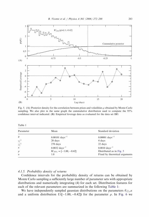
Uð½smin; smax�Þ to be uniform representing our level of ignorance on the acceptabledispersion of deviations between data and model. Having specified ignorance priorsand likelihood (28), we evaluate posterior (27) by Monte Carlo sampling. In Fig. 5we show the resulting posterior probability density and find the 95% confidenceinterval to be IC95%ðrÞ ¼ ½�1:00;�0:42�, what is strong evidence for an asymmetricprobability density of returns.

ARTICLE IN PRESS

Table 1

Parameter Mean Standard deviation

y 0:00101 days�1 0:00001 days�1

g�1120 days 4 days

g�12270 days 22 days

k 0:0032 days�1 0:0010 days�1

r IC95% ¼ ½�1:00;�0:42� Distributed as in Fig. 5

a 1:0 Fixed by theoretical arguments

-1 -0.75 -0.5 -0.25 00

0.5

1

2

3

p(ρ|

L)

0 5 10 15 20Lag (days)

-8

-6

-4

-2

0

2

4

Em

piri

cal L

ever

age

IC95%(ρ)=[-1,-0.42]

Cummulative posterior

(A)

(B)

Fig. 5. (A): Posterior density for the correlation between prices and volatilities r obtained by Monte Carlo

sampling. We also plot in the same graph the cummulative distribution used to compute the 95%

confidence interval indicated. (B): Empirical leverage data as evaluated for the data set IB3.


4.1.5. Probability density of returns

Confidence intervals for the probability density of returns can be obtained byMonte Carlo sampling a sufficiently large number of parameter sets with appropriatedistributions and numerically integrating (4) for each set. Distribution features foreach of the relevant parameters are summarized in the following Table 1:

We have independently sampled gaussian distributions on the parameters y,g1,kand a uniform distribution Uð½�1:00;�0:42�Þ for the parameter r. In Fig. 6 we

ARTICLE IN PRESS

-1 -0.8 -0.6 -0.4 -0.2 0 0.2 0.4 0.6 0.8 1 1.2X

p(x)

1 day

5 days

20 days

40 days

80 days

160 days

Fig. 6. Log-linear plot of empirical and theoretical probability densities of returns. Circles represent, from

bottom to top, empirical densities at respectively 1; 5; 20; 40; 80 and 160 days. Full lines indicate 95%

confidence intervals obtained by numerical integration at Monte Carlo sampled parameter values.

Densities at distinct time scales are multiplied by powers of 10 for clarity of presentation.

6040200 80 100

Lag (mins)

-0.1

0.0

0.1

Aut

ocor

rela

tion

Func

tion

2001200220032004

Fig. 7. Intraday autocorrelation function for each year composing the dataset IB2. The time scale

separating micro- and mesoeconomic phenomena is shown to be of about 20min.


compare empirical probability densities with theoretical confidence intervals at 95%finding a clear agreement at time scales ranging from 1 to 160 days.

4.2. High frequency

4.2.1. Autocorrelation of intraday returns

Our main aim is to describe the fluctuation dynamics at intermediate time scales offormed prices (mesosconomic time scales) by a model which assumes uncorrelatedreturns. The price formation process occurs at time scales from seconds to a fewminutes where the placing of new orders and double auction processes take place.We propose to fix the shortest mesoeconomic time scale to be the point where theintraday autocorrelation function vanishes. In Fig. 7 we show that the intraday

ARTICLE IN PRESS


return autocorrelation function vanishes at about 20min for each of the 4 yearscomposing data set IB2. We, therefore, consider as mesoeconomic time scales over20min.

4.2.2. Effective duration of a day

At first glance, it is not clear whether intraday and daily returns can be describedby the same stochastic dynamics. Even less clear is whether aggregation fromintraday to daily returns can be described by the same parameters. To verify thislatter possibility we have to transform units by determining the effective duration inminutes of a business day Teff . This effective duration must include the daily tradingtime at the Sao Paulo Stock Exchange and the impact of daily and overnight gapsover the diffusion process. The Sao Paulo Stock Exchange opens daily for electronictrading from 10 a.m. to 5 p.m. local time and from 5:45 p.m. to 7 p.m. for after-market trading, totalizing 8 h 15min of trading daily.

To estimate Teff in minutes we observe that the daily return variance vð1dÞ is theresult of the aggregation of 20min returns, so that, considering a diffusive process,we would have

vð1dÞ ¼Teff

20vð20 minÞ . (29)

It has been already observed that the volatility fluctuation dynamics aremean reverting with at least two time scales g�11 � 20 days and g�12 � 1 year.Considering the longest relaxation time we estimate Teff by estimating the meandaily volatility for each one of the years in IB2. In Fig. 8A we show linear regres-sions employed for estimating the mean daily variance vð1dÞ for each year inIB2 following the procedure described in Section 4.1.1. In Fig. 8B we showlinear regressions employed to estimate vð20 minÞ, the effective duration confi-dence intervals are obtained from (29). The mean 95% confidence interval overthe 4 years analysed results in IC95%ðTeff Þ ¼ ½9 h10 min; 9 h56 min� what isconsistent with 8 h 15min of daily trading time plus an effective contribution ofdaily and overnight gaps.

4.2.3. Probability density of intraday returns

For evaluating the probability density of intraday returns we have re-estimated themean volatility y and the amplitude of volatility fluctuations k along the period2001–2004 represented in the data set IB2. We then have rescaled the dimensionalparameters as yðIDÞ

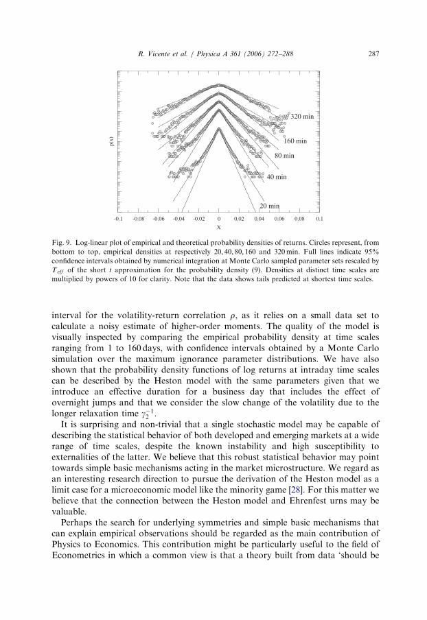
¼ y=Teff , gðIDÞ ¼ g=Teff and kðIDÞ ¼ k=Teff . Having rescaled thedistributions describing our ignorance on the appropriate returns we have em-ployed Monte Carlo sampling to compute confidence intervals for the short-timelags approximation of the theoretical probability density described in (9). In Fig. 9we compare the resulting confidence intervals and the data. We attain reasonablygood fits for the longer time scales, as we approach the microeconomic timescales the theoretical description of the tails breaks with the empirical data showingfatter tails.

ARTICLE IN PRESS

0 5 10 15Lag (days)

0

8×10-3

6×10-3

4×10-3

2×10-3

6×10-5

4×10-5

2×10-5

c 2(t

)c 2

(t)

2001200220032004

20 30 40 50 60 70Lag (mins)

0

(10h00’, 11h00’)(7h30’, 8h40’)(7h30’, 8h50’)(10h40’,12h23’)

(B)

(A)

Fig. 8. (A): Second cumulant of returns c2ðtÞ versus the time lag in days for each year composing IB2 is

used to estimate the mean daily variance vð1dÞ following the procedure described in Section 4.1.1. (B): Plots

of intraday second cumulants c2ðsÞ of returns versus the time lag from 20 to 80min employed to estimate,

via linear regression, the 20min variance vð20 minÞ. Resulting Teff 95% confidence intervals are also shown

in the figure.


5. Conclusions and perspectives

We have studied the Heston model with stochastic volatility and exponential tailsas a model for the typical price fluctuations of the IBOVESPA. Prices have beencorrected for inflation and a period spanning the last 15 years, characterized bymemoryless returns, have been chosen for the analysis. We also have expunged fromdata a drawdown inconsistent with the supposition of independence made by theHeston model that took place in the transition between the first 22 years of longmemory returns to the memoryless time series we have analysed.

The long-term mean volatility y has been estimated by observing the time scalingof the log-returns variance. The relaxation time for mean reversion g�1 has beenestimated by observing the autocorrelation function of the log returns variance. Wehave verified that a modified version of the Heston model with two very differentrelaxation times (g�11 � 20 days and g�12 � 1 year) is required for describing theautocorrelation function correctly. We have used the minimum requirement for anon-vanishing volatility aX1 to calculate the scale of the variance fluctuation k.Finally, we employed the Bayesian statistics approach for estimating a confidence

ARTICLE IN PRESS

-0.1 -0.08 -0.06 -0.04 -0.02 0 0.02 0.04 0.06 0.08 0.1

X

p(x)

20 min

40 min

80 min

160 min

320 min

Fig. 9. Log-linear plot of empirical and theoretical probability densities of returns. Circles represent, from

bottom to top, empirical densities at respectively 20; 40; 80; 160 and 320min. Full lines indicate 95%

confidence intervals obtained by numerical integration at Monte Carlo sampled parameter sets rescaled by

Teff of the short t approximation for the probability density (9). Densities at distinct time scales are

multiplied by powers of 10 for clarity. Note that the data shows tails predicted at shortest time scales.


interval for the volatility-return correlation r, as it relies on a small data set tocalculate a noisy estimate of higher-order moments. The quality of the model isvisually inspected by comparing the empirical probability density at time scalesranging from 1 to 160 days, with confidence intervals obtained by a Monte Carlosimulation over the maximum ignorance parameter distributions. We have alsoshown that the probability density functions of log returns at intraday time scalescan be described by the Heston model with the same parameters given that weintroduce an effective duration for a business day that includes the effect ofovernight jumps and that we consider the slow change of the volatility due to thelonger relaxation time g�12 .

It is surprising and non-trivial that a single stochastic model may be capable ofdescribing the statistical behavior of both developed and emerging markets at a widerange of time scales, despite the known instability and high susceptibility toexternalities of the latter. We believe that this robust statistical behavior may pointtowards simple basic mechanisms acting in the market microstructure. We regard asan interesting research direction to pursue the derivation of the Heston model as alimit case for a microeconomic model like the minority game [28]. For this matter webelieve that the connection between the Heston model and Ehrenfest urns may bevaluable.

Perhaps the search for underlying symmetries and simple basic mechanisms thatcan explain empirical observations should be regarded as the main contribution ofPhysics to Economics. This contribution might be particularly useful to the field ofEconometrics in which a common view is that a theory built from data ‘should be

ARTICLE IN PRESS


evaluated in terms of the quality of the decisions that are made based on the theory’[29]. Clearly, these two approaches should not be considered as mutually exclusive.

Acknowledgements

We thank Victor Yakovenko and his collaborators for discussions and forproviding useful MATLAB codes. We also wish to thank the Sao Paulo StockExchange (BOVESPA) for gently providing high-frequency data. This work hasbeen partially (RV,VBPL) supported by FAPESP.

References

[1] J.P. Fouque, G. Papanicolaou, K.R. Sircar, Derivatives in Financial Markets with Stochastic

Volatility, Cambridge University Press, Cambridge, 2000.

[2] J. Hull, A. White, J. Finance 42 (1987) 281.

[3] E.M. Stein, J.C. Stein, Rev. Finan. Stud. 4 (1991) 727.

[4] S.L. Heston, Rev. Finan. Stud. 6 (1993) 327.

[5] B.M. Roehner, Patterns of Speculation, Cambridge University Press, Cambridge, 2002.

[6] P. Mirowski, More Heat than Light, Cambridge University Press, Cambridge, 1989.

[7] R.N. Mantegna, H.E. Stanley, An Introduction to Econophysics, Cambridge University Press,

Cambridge, 2000.

[8] A.A. Dragulescu, V.M. Yakovenko, Quant. Finance 2 (2002) 443.

[9] A.C. Silva, V.M. Yakovenko, Physica A 324 (2003) 303.

[10] A.C. Silva, R.E. Prange, V.M. Yakovenko, Physica A 344 (2004) 227.

[11] R.F. Engle, A.J. Patton, Quant. Finance 1 (2001) 237.

[12] J.-P. Bouchaud, A. Matacz, M. Potters, Phys. Rev. Lett. 87 (2001) 228701-1.

[13] J. Perello, J. Masoliver, Phys. Rev. E 67 (2003) 037102.

[14] M. Boguna, J. Masoliver, Preprint, cond-mat/0310217 (2003).

[15] B. LeBaron, J. Appl. Econom. 7 (1992) S137.

[16] T. Di Matteo, T. Aste, M.M. Dacorogna, J. Banking Finance 29 (2005) 827.

[17] B. LeBaron, Quant. Finance 1 (2001) 621.

[18] H. Takahashi, Physica D 189 (2004) 61.

[19] S. Shreve, Lectures on stochastic calculus and finance.

[20] BOVESPA Index, http://www.bovespa.com.br.

[21] Fundac- ao Getulio Vargas, http://www.fgvdados.fgv.br.

[22] A.C. Harvey, A. Jaeger, J. Appl. Econom. 8 (1993) 231.

[23] R.L. Costa, G.L. Vasconcelos, Physica A 329 (2003) 231.

[24] A. Johansen, D. Sornette, Eur. Phys. J. B 1 (1999) 141.

[25] J. Perello, J. Masoliver, J.-P. Bouchaud, Appl. Math. Finance 11 (2004) 27.

[26] O.E. Barndorff-Nielsen, N. Shephard, J. Roy. Stat. Soc. 63 (2) (2001) 167.

[27] D.S. Sivia, Data Analysis: A Bayesian Tutorial, Oxford University Press, Oxford, 2000.

[28] D. Challet, M. Marsilli, Y.-C. Zhang, Minority Games, first ed., Oxford University Press, Oxford,

2004.

[29] C.W.J. Granger, Empirical Modelling in Economics, first ed., Cambridge University Press,

Cambridge, 1999.

http://www.bovespa.com.br

http://www.fgvdados.fgv.br

underlying dynamics of typical fluctuations of an emerging market price index: the heston model from...

Documents