- 1 -

School of Sciences

Faculty of Geosciences

Undergraduate Thesis:

Seismotectonic Characterization of the Colombian Pacific

Region: Identification of Tectonic Patterns Through

Geostatistical Analysis

María Daniela Gracia

201222439

Director: Fabio Iwashita

____________________

Co-Director: Jean Baptiste Tary

____________________

November 24/2017

- 2 -

I wish to thank my mother Pilar, father Daniel and sisters Manuela and Sara for

being a constant source of help and encouragement. Special thanks to my lovely

boyfriend Jesse for supporting me and helping me believe in myself and to

friends who have supported me throughout the process. And finally, I wish to

thank the faculty of geosciences and my professors Fabio Iwashita and Jean

Baptiste Tary for their motivation, disposition to help and great knowledge.

- 3 -

Abstract

Earthquake occurrence is a consequence of many processes within the

Earth such as tectonic stress loading, fluid diffusion or static stress

triggering. As a result of this, patterns of spatial and temporal

distribution, that earthquakes have historically displayed, keep the

footprint of the mechanisms that give them origin. Quantifying these

patterns and the extent of the causality and correlation between seismic

events is then an interesting and useful subject of study. It is useful

because it opens the doors to more accurate estimations of the behavior

of earthquakes, which inherently decreases the risk of catastrophes. The

Colombian Pacific region is a zone that presents a high degree of

geological complexity, it lies parallel to a trench where the Nazca plate

subducts below the South American Plate, which inherently results in

increased seismic activity and rupture. In this study a sequence of 134

events that happened in this zone in a period of 68 months is studied.

These earthquakes are organized in complex spatial structures that were

separated trough clustering analysis and then subjected to geostatistical

analysis. The geostatistical analysis consisted of: an evaluation of the

distribution of events as a function of time and a semivariogram analysis,

by which the degree of correlation between events was studied. The

interaction within these events is highly complex but, to some extent,

some system wide correlations are observed. As opposed to what was

initially expected, the semivariogram analysis did not manage to measure

the degree of correlation for this particular sequence. What this means

is that all semivariograms lie within a zone that denotes no-correlation

and present a generalized uncorrelated form.

- 4 -

Resumen

La ocurrencia de terremotos es la consecuencia de los múltiples

procesos que ocurren en el interior de la Tierra como lo son la carga

tectónica por esfuerzo, la difusión de fluidos o el desencadenamiento por

esfuerzo estático. Como resultado de esto, los patrones de distribución

espacial y temporal que los terremotos han mostrado históricamente guardan

la huella de los mecanismos que los originan. Cuantificar dichos patrones

y la extensión de la causalidad y correlación entre eventos sísmicos es

por lo tanto una materia de estudio útil e interesante. Es útil ya que

abre las puertas a un área de estudio donde las estimaciones del

comportamiento de los terremotos adquieren mayor precisión, lo cual

inherentemente reduce el riesgo de catástrofes. La región Pacífica de

Colombia es una zona que presenta un alto grado de complejidad en su

geología, yace paralela a una trinchera donde la placa Nazca subduce por

debajo de la placa Sur Americana, lo que automáticamente resulta en una

mayor actividad sísmica y en ruptura. En este estudio se considera una

secuencia de 134 eventos que ocurrieron en esta zona en un periodo de 68

meses. Estos terremotos se organizan en estructuras espaciales complejas,

dichas estructuras fueron separadas por medio de análisis de clusters y

luego analizadas usando métodos geoestadísticos. El análisis

geoestadístico consistió de: La evaluación de la distribución de los

eventos como función del tiempo y un análisis de semivariogramas, por

medio del cual el grado de correlación entre los eventos fue estudiado.

La interacción entre los eventos estudiados es de alta complejidad, sin

embargo, hasta cierto punto es posible observar correlaciones a lo largo

de todo el sistema. A diferencia de lo que se esperaba, el análisis por

medio de semivariogramas no logró medir el grado de correlación para esta

secuencia particular. Lo que esto significa es que todos los

semivariogramas experimentales obtenidos se encuentran dentro de una zona

que denota ausencia de correlación y en general presentan una forma que

no muestra relación entre la causalidad de los eventos.

- 5 -

Table of Contents

1. Chapter 1. Introduction (6)

2. Chapter 2. Geology of the Colombian Western Margin (8)

2.1 Geological Setting (8)

2.2 Tectonic Setting (10)

2.2.1 Tectonic Background (14)

2.3 Main fault systems (17)

2.4 Seismicity (21)

2.4.1 Colombian National Seismic Network (Red Sismológica

Nacional de Colombia) (21)

2.4.2 Historical seismicity (21)

2.4.3 General Characteristics of Seismicity (24)

3. Chapter 3: Theoretical Framework

(31)

3.1 Seismology Framework (31)

3.1.1 Focal Mechanisms (31)

3.2 Geostatistical Framework (34)

3.2.1 Geostatistics (34)

3.2.2 Preliminary Definitions (36)

3.2.3 Semivariogram Analysis (38)

3.2.4 Cluster Analysis: K-Means (40)

4. Chapter 4. Data Selection, Processing and Methodology (42)

4.1 Data Selection, Variable Overview and Exploratory Analysis (42)

4.2 Spatial and Temporal Classification of Earthquakes:

Clustering of the Data (44)

4.2.1 Spatial Clustering Results (49)

4.2.2 Temporal Clustering Results (51)

4.3 Distribution of Earthquakes as a Function of Time (52)

- 6 -

4.4 Semivariogram Analysis of the Data (53)

4.4.1 Correlation of Earthquakes on Individual Features (55)

4.4.2 Correlation of Earthquakes in the System (57)

4.5 Focal Mechanisms (58)

5. Chapter 5. Results, Discussion and Conclusions (58)

5.1 Clustering of the Data (58)

5.2 Fault Interaction - Earthquakes as a Function of Time (60)

5.3 Correlation of Earthquakes on individual Faults and

in the System: Evaluation of Semivariogram Functions (62)

5.4 Conclusions (63)

6. Appendix A. Spatial Clustering Characteristics (66)

7. Bibliography (69)

- 7 -

1. Chapter 1. Introduction.

Subduction zones have four main types of associated events: (1) shallow

events occurring in the crust, (2) intraplate events due to bending of the

subducting slab ahead of the trench, (3) large intraplate events and (4)

deep events associated to the Wadati-Benioff zone (Scawthorn & Chen, 2002).

The seismicity of the Western Colombian Margin (WCM), where the Nazca Plate

subducts below the South American Plate, has been predominantly studied in

terms of the associated Wadati-Benioff zones, large intraplate events,

seismic nests (Cauca and Bucaramanga),current state of stress, seismic hazard

and slab geometry (Barazangi & Issacks, 1976; Suárez, Molnar & Burchfiel,

1983; Wysession, Okal & Miller, 1991; Taboada,2000; Chen, Bina & Okal, 2001;

Rietbrock & Waldhauser, 2004; Pedraza Garcia, Vargas & Monsalve, 2007;

Pararas-Carayannis, 2012; Castilla & Sánchez, 2014; Salcedo-Hurtado & Pérez,

2016, Wagner et al, 2017.) Although it is known that seismicity in the region

surrounding the trench (type 1 and 2 events) is mostly associated to active

tectonic features, a more in depth study, that properly groups the events,

associates them to different structures and quantifies their characteristics,

is yet to be developed.

It is well known that earthquake occurrence is not randomly distributed,

instead it is a phenomenon that when observed over long temporal and spatial

scales behaves in a coherent and structured manner (Walsh and Watterson,

1991; Nicol et al., 2006.). As a realization of this, historical seismicity

has shown evidence of both spatial and temporal clustering (Plafker & Savage,

1970; Stein et al, 1997). This behavior is directly linked to the conduct of

- 8 -

the mechanisms triggering the seismic events (tectonic static stress

triggering, fluid migration and extraction, etc.). Therefore, given that

seismic behavior does not occur randomly, geostatistics becomes a great tool

in order to quantify its characteristics.

Geostatistics have been developed in order to model and evaluate natural

resources and phenomena, its main assumption is that spatial auto correlation

exists (Olea, 2006). It is a useful approach at quantifying seismic

information, given that it helps measure the extent and behavior of spatial

correlation through tools such as the semivariogram. Some authors have

applied this methodology to different areas of seismic study; Şen (1998)

used semivariograms in order to identify heterogeneities in regional

seismicity of Turkey and Shaefer et al. (2014) used clustering algorithms in

order to separate background seismicity form triggered seismicity.

Mouslopoulou & Hristopulos (2011) analyzed an entire earthquake sequence

through semivariogram analysis and manage d to identify and measure system

wide correlations. The latter study is particularly interesting given that

it can lead to the quantification of interesting and useful spatio-temporal

variables in a broad variety of scenarios. For this reason, the methodology

proposed by Mouslopoulou & Hristopulos (2011) is the one that guides this

project.

In the present study the goal is to identify and explore the existence of

spatiotemporal patterns in seismic data from the Colombian Western Margin

and based on this answer questions pertaining: the (1) structure of

earthquake activity in space and time; (2) earthquake interaction along

individual tectonic features; (3) system wide earthquake interaction; (4)

interaction between different tectonically active structures. This will be

- 9 -

achieved through: (a) spatio-temporal evaluation, (b) clustering procedures

and (c) semivariogram analysis. Additionally, some focal mechanism solutions

will be considered when performing the evaluation of the results. The paper

is structured as follows: (I) geological, tectonic and seismic

characterization of the region, (II) theoretical framework and (III) data

selection, processing and analysis.

2. Chapter 2. Geology of the Colombian Western Margin.

2.1 Geological Setting.

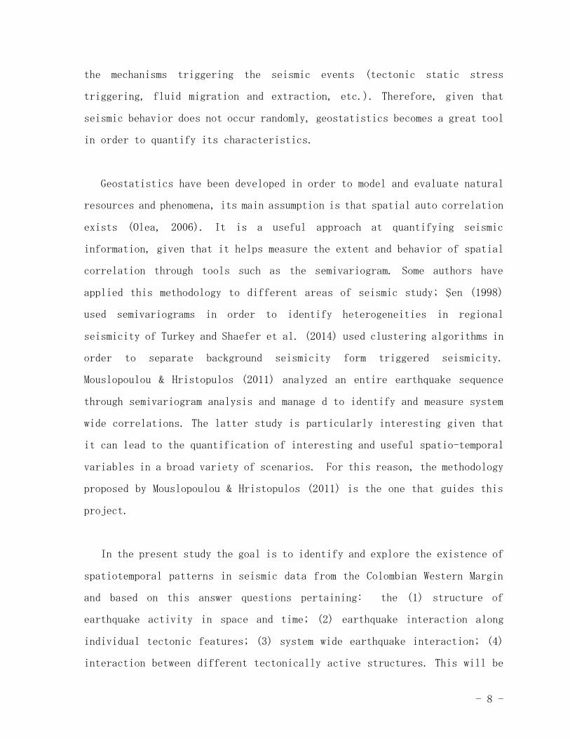
The Colombian territory (Figure 1) is located on the northwestern part of

South America and consists of two main regions; The eastern portion, which

is mainly a plain terrain covered by savannah, fragmented forests at the

north and tropical forests at the south and the western portion dominated by

the Andes mountain ranges and also the subject of this study. The Colombian

Andes consist of 3 mountain ranges; the Western Cordillera, Central

Cordillera and Eastern Cordillera. The Western and Central Cordillera are

separated by the Cauca-Patía Valley and are trending in a SW-NE direction,

following the Pacific coastline. The Central and Eastern Cordillera are

separated by the Magdalena Valley, at this point the Eastern Cordillera turns

towards the east. Additionally, the Romeral Fault System located between the

Cauca- Patía Valley and the Central Cordillera provides an additional

division for the Colombian Andes resulting in the Western and Eastern Andes,

respectively.

- 10 -

The Western Andes region is characterized by oceanic rocks that were

accreted to the continent during the Mesozoic and Cenozoic periods; The

Western Cordillera is composed of turbiditic deposits and ophiolites whilst

the Serranía del Baudó, a smaller mountain range located near the northern

tip of the Western Cordillera, presents island arc composition (Taboada et

al, 2000).The Eastern Andes (Central and Eastern Cordillera) are

characterized by rock formations that have experienced several phases of

deformation (Mégard, 1987); The Central Cordillera consists of a

polymetamorphic (medium to low pressure metamorphism) basement (oceanic and

continental) of Paleozoic age intruded by a series of plutons of Mesozoic

and Cenozoic age, as well as active volcanism along its crest. The Eastern

Cordillera also consists of a polymetamorphic basement (Precambrian and

Paleozoic) that experienced deformation in multiple pre-Mesozoic orogenic

events (Taboada et al, 2000), above the basement there is a Mesozoic and

Cenozoic sedimentary sequence that was highly deformed in the Neogene

(Irving, 1971).

- 11 -

Figure 1. Topographic map of Colombia showing the Colombian Andes and political boundaries.

(Source IGAC1)

2.2 Tectonic Setting.

Colombia is bounded by active tectonic margins in all of its coastal

regions; In the north coast the Caribbean plate is moving in a E - SE trend

with respect to South America creating an accretionary wedge and in the

western coast (Pacific) the Nazca plate is subducing in a W-E trend forming

a trench that extends for 500 to 1000 km (Norabuena et al, 1998). The rate

of convergence of the Nazca and Caribbean plates (relative to South America

plate) at a given location can be calculated by using the UNAVCO Plate Motion

1Geographical Institute Agustin Codazzi; Colombian entity in charge of the country’s

cartography.

- 12 -

Calculator2 where the different models of relative plate motions are

available. At a latitude of 4.5° north and longitude of 79° west the rate of

convergence for Nazca is of 5.29 𝑐𝑚/𝑦𝑟 with an azimuth of 𝑁 80.2 𝑊. As for

the Caribbean plate, at a latitude of 10.7° north and longitude of 76° west

it is moving at a rate of 2.60 𝑐𝑚/𝑦𝑟 with an azimuth of 𝑁 58.4 𝐸 (Kremmer,

Blewitt and Klein, 2014).

In the Early Miocene the Farallon Plate underwent a rupture process that

divided the plate into Cocos and Nazca. The splitting of the Farallon plate

began in the Eocene and Oligocene (Atwater, 1989), when the Vancouver and

Monterey plates detached due to pull of the California subduction zone. As

for the bigger detachment (Cocos- Nazca), it was a result of: (1) An

increasingly divergent slab pull at the Central and South American subduction

zones below the South American plate, (2) previous detachments and (3)

weakening of older portions of the plate associated to the Galapagos hotspot

in the Late Oligocene (Lonsdale, 2005). After the rupture a spreading center

rapidly evolved, later acquiring a direction parallel to the divergence of

Cocos and Nazca plates (N-S).

The resulting Nazca plate contains evidence of stress-induced processes

that occurred pre and post rupture, they manifest themselves as ridges and

tears (Figure 2 (a)); although the correlation within the mechanisms is still

under interpretation, Lonsdale (2005) provides a reasonable explanation.

Bordering the Malpelo Island is the Malpelo Rift, now a fossil spreading

2This facility is supported by the National Science Foundation and NASA and it allows for the

calculation of plate convergence rates and azimuths at a given magnitude. It can be used with

different plate motion models, in this case the rates given correspond to the GSRM v2.1 (Kremmer,

Blewitt and Klein, 2014).

- 13 -

center, that remained active until about 8.5 Ma, linked to this structure is

the Sandra Ridge (Late Miocene), an equally abandoned spreading center. The

Sandra Ridge (~ 5° 𝑁) presents active seismicity with focal mechanisms

suggesting both strike–slip and normal faulting, the latter being less

common, which has led to believe that it is undergoing reactivation

(Lonsdale, 2005) as a spreading center that will eventually tear the Nazca

plate (Boer et al 1998; Vargas & Mann, 2013). Lonsdale (2005) suggests that

the Sandra Rift was a Cocos-Nazca spreading axis that translated west from

12 to 9 Ma, it eventually overlapped with the eastern segment of the Malpelo

Rift which caused the spreading to slow down.

The geometry of the slab subducing below the Colombian Pacific trench is

a matter of debate, the main observations are (1) an E-W discontinuity that

marks an abrupt change in the angle of subduction near latitude 5° 𝑁, bounded

by low angle subduction northward and normal, or more steep, subduction

southward and (2) intermediate depth seismicity in the Bucaramanga Seismic

Nest (BSN) near latitude 6° 𝑁. Different models suggest different processes

of interaction at depth and have been developed from tectonic evidence and

tomographic and earthquake relocation techniques.

Taboada et al (2000) suggests that the region is experiencing an overlap

of slabs at depth where the northern portion corresponds to the Paleo-

Caribbean Plateau (PCP) and the southern portion to normal Nazca subduction.

Both separated by a massive EW transform shear zone located at latitude

5.2° 𝑁, additionally the author explains the BSN as an inflexion zone in the

PCP (Figure 2 (b)). Ojeda & Havskov (2001) don’t find evidence of a tear,

based on observed geometry they describe two contingent subduction zones,

the Cauca Subduction Zone (south) (CSZ) and the Bucaramanga Subduction Zone

- 14 -

(north) (BSZ) that interact at depth. The CSZ is associated to Nazca

subduction and has an angle of 35°, and the BSZ has an unclear origin with

an angle of 40° in its southern portion and 27° in its northern portion,

both areas are linked by a gradual change in geometry.

Other authors do suggest that the discontinuity is a tear within Nazca,

Vargas & Mann (2013) describe it as a tear, or Caldas Tear as they name it,

that extends for ∼ 240 𝑘𝑚 at latitude 5.6° 𝑁. It separates a zone of shallow

(20°– 30°), southeastward subduction to the north that extends up to 11° 𝑁

with a WBZ located at > 300 𝑘𝑚 form the trench from a zone of steeper

(30°– 40°) subduction, associated with an active NS chain of active arc

volcanoes to the south which directly underlies the active Andean arc (Figure

2 (c)) (Vargas & Mann, 2013; Jaramillo et al, 2017). The proposed Caldas

Tear penetrates the upper crust acting as a fault zone and is aligned with

the inactive Sandra ridge (Figure 2 (a)), for this reason it has been

suggested that a portion of this ridge subduced, weakened and evolved into

a tear.

Chiaraba et al (2015) rephrases the issue as an abrupt offset of the

Wadatti-Benioff zone at 5.8 N and suggests that the Nazca plate is segmented

by an EW slab tear. The BSN is presented as an increase in the angle of

subduction below the Eastern Cordillera where massive dehydration and

eclogitization processes take place. Additionally, for this author it is

important evidence that the tear is aligned with the Coiba Transform Fault

(Figure 2 (a)), suggesting that the same structure evolved into a slab tear.

Finally, Jaramillo et al (2017) have managed to better characterize history

of the Pacific Margin by compiling volcanic ages and locations, they find

- 15 -

that: (a) Between 14 and 9 Ma there was a continuous arc along the entire

Pacific Margin directly attributed to Nazca subduction, (b) by 6 Ma a fully

formed flat slab was already developed, it initially extended further to the

south than it does today and (c) the current geometry has been present since

~4 Ma, therefore the Nazca Plate must comprise at least part of the northern

flat slab.

Figure 2. a) Revised interpretation of the pattern of crustal isochrons and abandoned plate

boundaries in the eastern Panama basin as well as main geological structures of the Nazca

plate including the Malpelo and Sandra rifts. (Source: Lonsdale, 2005). b) Schematic

tectonic cross section of the Northern Andes and Caribbean illustrating the geodynamic

pattern after collision of the Baudó Panama island arc. (Source: Taboada et al, 2000). c)

Schematic 3D model suggesting flat subduction on the northern side of the weakness zone

formed by the Sandra rift and the Caldas tear. (Source: Vargas & Mann, 2013)

2.2.1 Tectonic Background.

In a geological context this region (western Colombia and surroundings)

is identified as the Northern Andean Block. The Northern Andean Block can be

- 16 -

separated in four lithotectonic3 realms, these realms are non-homogeneous

structures that are grouped due to their genetic history (From Mesozoic-

Cenozoic4 to present) and development (Cediel, Shaw and Cáceres, 2003). The

ones relevant to this study are the Guiana Shield Realm, Central Continental

Sub-Plate Realm and, most importantly, the Western Tectonic Realm. (Figure

3)

Guiana Shield Realm

This terrain is made up of the Precambrian and autochthonous Guiana

Shield, including northeastern Colombia, the eastern foreland front of the

Eastern Cordillera and the Amazon basin. In this area have been identified

collision, collision, penetrative deformation and high grade metamorphism

during the Grenville orogeny (Pre-Andean) (Cediel, Shaw & Cáceres, 2003).

Central Continental Sub-Plate Realm (CCSP)

This realm is made up of the central territory of the northern Andes

including the Central and Eastern Cordilleras as well as the Magdalena

Valley; The terrains of Precambrian and Paleozoic age are considered to be

mostly allochtonous whilst Mesozoic to recent portions are considered to be

autochthonous. This territory contains evidence of multiple pre-Andean

geological events including a middle Ordovician-Silurian Cordillera type

orogeny as well as deep crustal rifting during the Late Jurassic to Cretaceous

3 Lithotectonic Unit refers to a geological region or domain that has been formed and/or deformed

by a distinctive tectonic environment.

4 The Mesozoic- Cenozoic period of the Northern Andean Block is characterized by accretions,

deformations, uplift, and magmatism (Cediel, Shaw and Cáceres, 2003).

- 17 -

in the inverted sedimentary basin of the Eastern Cordillera. (Cediel, Shaw

& Cáceres, 2003).

Western Tectonic Realm (WTR)

The WTR is the most relevant to this study, it is a result of the

convergence of the Nazca and South America plates in the western margin of

Colombia, it is made up of the region that encloses the Western Cordillera

and is considered to be allochtonous. It consists of fragments of the Pacific

oceanic plateau, aseismic ridges, ophiolites and island arcs that have been

organized in three main terrains: Pacific Asemblage Terrain (PAT), Caribbean

Terranes (CAT) to the north and the Choco Arc Terrain (CHO) in the northwest.

The PAT includes Romeral, Dagua-Piñon and Gorgona terrains, they consist

of a variety of oceanic complexes including mafic and ultramafic sequences,

ophiolites, oceanic sediments, basalts, pillow lavas and gabbros and are

dated from the Late Jurassic to Late Cretaceous. The CAT contains the San

Jacinto and Sinú terrains; The first one presents northeast structural trend

while the latter has a strike and slip structural pattern within a magnetic

basement, the oldest structures in the territories are from the Paleocene

and Oligocene respectively. The CHO contains Cañas Gordas and Baudó and a

northeast oriented vergence. Both terrains are characterized by the

alternation of oceanic sediments and volcanic rocks (basalts), however, Cañas

Gordas contains a few intrusions dated in the Late Cretaceous and more

recently in the Eocene, the intrusions occurred prior to the accretion of

the terrain to the continental land (Cediel, Shaw & Cáceres, 2003).

- 18 -

Figure 3. Lithotectonic and morphostructural map of northwestern South America; (Source:

Cediel, Shaw, & Cáceres, 2003)

2.3 Main Fault Systems.

Given that the Northern Andean Block is made up of a conjunction of

autochthonous and allochtonous terrains of different origins and ages an

- 19 -

important fault system must be present to account for this. The Colombian

fault system is large and highly complex and it must be noted that strike-

slip faulting is the dominant faulting mechanism; the following are the most

important fault systems relevant to this study as detailed by Cediel, Shaw

& Cáceres, 2003. (Figure 4).

Figure 4. a) Main fault system distribution in Colombia. (Source: Ojeda & Havskok). b)

West-east transect across the Colombian Andes. Principal sutures: 1 = Grenville (Orinoco)

Santa Marta–Bucaramanga–Suaza faults; 2 = Ordovician-Silurian Palestina fault system; 3 =

Aptian Romeral-Peltetec fault system; 4 = Oligocene-Miocene Garrapatas-Dabeiba fault system;

5 = late Miocene Atrato fault system. (Source: Cediel, Shaw, & Cáceres, 2003)

Bucaramanga – Santa Marta Fault System

Active during the Grenville Orogeny, later reactivated in the Aptian-

Albian and currently active and associated to the Bucaramanga Seismic Nest.

This fault system is a paleosuture that links a portion of the CCSP to the

Guiana Shield, it displays a dominant left lateral displacement, with a total

lateral displacement in the order of 40 km (Toro, 1990) and a total

- 20 -

displacement of over 100 km (Rodríguez, 1985). Given that it is a paleosuture

it presents deep crustal penetration as well as some magmatism located at

the south of the seismic nest of Pliocene-Pleistocene age (Cediel and

Cáceres, 2000).

Suaza Fault System

It corresponds to the paleosuture that links the southern portion of the

CCSP to the Guiana Shield and is connected to the Bucaramanga fault in the

subsurface of the Eastern Cordillera. This fault system reactivated in the

Neogene, which resulted in series of associated right-lateral oblique thrust

faults (Velandia et al, 2001).

Llanos Fault System

This term refers to the group of faults that formed a thrust front and

allowed the Eastern Cordillera to position itself over the foreland sequences

of the Llanos basin. It consists of at least three main thrust fronts one

below the other in a NS direction with a predominant NE strike (Cediel, Shaw

and Cáceres, 2003).

Palestina Fault System

This system includes multiple faults including the Chapetón- Pericos,

Ibague and Cucuana faults; it is a paleosuture for the Cajamarca and Valdivia

terranes. The faults associated to this system present right lateral strike-

slip displacement, evidence of shearing and merge into the Romeral fault

system towards the south (Cediel, Shaw and Cáceres, 2003).

Romeral – Peltetec Fault System

As it was previously mentioned, this system separates the western and

eastern Andes in Colombia. It is an important suture (paleo-continent margin)

where the oceanic Cretaceous territory of the Western Tectonic Realm meets

- 21 -

the CCSP and Guiana Shield, it has an extension of over 1000 km and its

activity began in the Triassic and Late Jurassic and reached a peak of

activity during the Upper Cretaceous (Vinasco & Cordani, 2012). This system

is complex and has a series of associated geological processes, which result

in an assortment of geological formations (Jurassic to Late Cretaceous) that

include: High degree metamorphic rocks such as eclogite and blueschist,

ophiolites, volcanic rocks, marine sediments and meta sediments and mafic

and ultramafic rocks. This fault system presents right lateral strike-slip

displacementin some of the associated faults and a dominantly NS strike

(Cediel, Shaw & Cáceres, 2003).

San Jacinto Fault System (Romeral North)

This is the northern extension of the Romeral Fault System, with the

distinction of absent subduction associated magmatism. It is the evidence of

the accretion of the Caribbean San Jacinto and Sinú terrains to the

continental margin (Cediel, Shaw & Cáceres, 2003).

Cauca Fault System

This fault system corresponds to the suture where the Romeral terrain

meets the oceanic terrains of Dagua-Piñón and outcrops in a large area. It

is dominantly of right-lateral strike-slip motion and presents west verging

thrust displacement in the sub surface (Cediel, Shaw & Cáceres, 2003).

Garrapatas-Dabeiba Fault System

It corresponds to the fault that separates the PAT from the CHO terrains

(Western Tectonic Realm), both oceanic, it’s origin has been suggested to

be an ancient transform fault from the Farallon plate during the Late Mesozoic

and Cenozoic (Barrero, 1997). It has also been linked to an already extinct

ridge within the Nazca plate and has facilitated the obduction of the Cañas

- 22 -

Gordas Terrain (CHO) (Cediel, Shaw & Cáceres, 2003).

Atrato Fault System

This suture system occurs within the Baudó terrain (CHO) and is

responsible for the obduction of the Baudó terrain above Cañas Gordas western

margin. It consists mainly of east verging echelon thrust faults (Cediel,

Shaw and Cáceres, 2003).

2.4 Seismicity.

2.4.1 Colombian National Seismic Network (Red Sismológica Nacional de

Colombia).

The National Seismologic Network of Colombia (RSNC) belongs to the

Colombian Geological Service, an important entity of the National Plan for

Disaster Attention and Prevention. It began proper activities in 1993 and

has grown ever since with the support of the Colombian and Canadian

governments as well as the United Nations. It has a total of 50 seismic

stations distributed in the Colombian territory and provides information on

all registered events, this is the agency that provided the data used in

this study

2.4.2 Historical Seismicity.

The history of seismicity in the Americas has its first records in the

mid late XV century, this records come from the Aztecs and the Colombian and

Venezuelan Indians, respectively (Ramirez, 1975). As for more concrete

- 23 -

documentation, the historical background goes back to the XVIII and XIX

centuries and consists of colonial documents containing personal annotations,

records and some early scientific studies from historians and scientists

(Espinosa, 2001). In the XX century more systematic studies began to take

place, the first seismic station was installed in Bogotá in the year 1923,

followed by a more modern station installed in 1941 and three more in 1948.

This was also the century in which the first Colombian historic seismic

catalogue was developed, it was published in 1975 by Jesús Emilio Ramírez

and is a compilation of sources including: international seismic catalogues,

scientific magazines, history books, newspapers, information provided by

peers, verbal data from witnesses and seismographic recordings.

Figure 5. Map showing the location of some historical seismic events in the Colombian

Pacific region. The events are labeled with their year of occurrence. Size indicates

magnitude.

- 24 -

The most significant seismic events that have taken place in the Colombian

Pacific can be seen in figure 5 and include (RSNC; Kanamori & McNally, 1962;

Ramirez, 1975; Herd et al., 1981; Espinosa, 2001; Espinoza, Gómez & Salcedo,

2004;)):

1906, January 1st, 10:36 am (local time, UTC-5): This event, considered as a

great earthquake, occurred along the Colombian Pacific coast and is a thrust

event associated to the subduction zone. Its moment magnitude is estimated

to be of 8.8 and it ruptured approximately 500 km of the earth in a NE

direction. It is notable for the tsunami it generated, whose magnitude has

been calculated to be of 8.7, bearing heights between 2 and 5 meters. The

tsunami and earthquake altogether resulted in a number of casualties between

1000 and 1500, multiple towns were destroyed and effects in nature such as

cracks, soil liquefaction and landslides were noted.

1970, September 26th, 07:02 am, 09:57 am, 10:38 pm (local time, UTC-5): This

series of three consecutive events did not cause any deaths, however they

destroyed Bahia Solano (a town in the Colombian Chocó region) almost

completely. Their respective moment magnitudes are 6.6, 5.4 and 6.5

1974, July 12th, 08:18 pm (local time, UTC-5): This event occurred in the

Darien province in the Pacific coastal region of Panamá near the Colombian

border in the Sambú fault. The main damage due to this event occurred in the

Chocó region of Colombia and Darién region in Panama. It’s moment magnitude

has been calculated to be of 7.1 at 10 km depth.

1976, July 11th, 11:56 am, 03:41 pm (local time, UTC-5): This events, both

superficial, occurred close to the Pacific coast of Panamá. The first one

only affected the Panamanian region and presented a smaller moment magnitude

of 6.8. The second one presented a moment magnitude of 7.3 and was felt

- 25 -

throughout Colombia, particularly in the Choco region, generating a small

Tsunami.

1979, December 12th, 02:59 am (local time, UTC-5): This massive earthquake

occurred in the Pacific coast and was felt in most of the Colombian territory

with particular focus in the Pacific region. It had an 8.1 moment magnitude

and occurred 80 km southwest of Tumaco at a depth of around 28 km. It had a

thrust mechanism and ruptured a 280 by 130 km zone, covering some of the

area already ruptured by the 1906 earthquake, in a N40W direction which

resulted in subsidence of 1.2 to 1.6 m along the segment. Additionally, a

tsunami that affected the entire coast all the way from Tumaco to Buenaventura

(200 km) occurred as a result of this event, it’s magnitude was calculated

to be 8.2 and the highest reported waves were of 2.5 m.

2004, November 15th, 04:06 am (local time, UTC-5): This event occurred near

Bajo Baudó in the Chocó region, damage extended all the way to Buenaventura,

Valle del Cauca and Cauca areas. It’s moment magnitude has been calculated

to be of 7.2 at depth of 16 km.

2.4.3 General Characteristics of Seismicity.

Colombian seismicity is complex and abundant, most of it occurs in the

Andean region and Pacific coast and is mainly linked to the subduction of

the Nazca plate. Some seismicity occurs in the Caribbean region and although

less studied, it is linked to the interaction between the Caribbean and South

American plates. Within a time lapse of 24 years (01/06/1993 to 01/06/2017)

a total of 164,868 seismic events have been recorded in the Colombian

territory and its close surroundings by the Red Sismológica Nacional de

- 26 -

Colombia (RSNC). As for the distribution in depth for these events 25.9 %

occur between 0 and 30 km (shallow), 4.9 % between 30 and 70 km, (shallow),

10.3 % between 70 and 120 km (intermediate), 58.7 % between 120 and 180 km

(intermediate) and less than 1 % for depths below 180 km (Figure 6).

Seismicity, as described by Ojeda & Havskov (2000), can be analyzed in

terms of shallow and deep seismicity in order to separate different features

and can be seen in Figure 6. Shallow seismicity (< 30 km) delineates the

main fault systems and tectonic boundaries in the crust. In the west most

seismic events are associated to the subduction of Nazca in the Colombian

Pacific trench, with most of the activity concentrated towards the south. In

the center of the country the seismicity is linked to the main fault systems

including Romeral and Cauca, where the major part of the seismic activity

takes place. High levels of shallow seismicity are observed in the eastern

portion of the Eastern Cordillera in the Salinas fault system (Figure 4.

(a)) and some is present in the northern portion of the Santa Marta-

Bucaramanga system. In the East, the Frontal fault system (Llanos Fault

system) (Figure 4. (a)) is the boundary between the Northern Andean block

and the South American Plate, additionally shallow seismicity fails to

delimit the boundary with the Caribbean territory (Ojeda & Havskov, 2000).

Deep seismicity (80 km – 200 km), on the other hand, is clustered in two

main spots: (1) in the Cauca Segment at the west (latitude: 3.2° − 5.6° 𝑁 and

longitude: 75.4° − 77.8°𝑊), linked to the subduction process between the

Nazca and South American plates and in the (2) Bucaramanga Segment at the

northeast (latitude: 5.0° − 9.5°𝑁 and longitude: 74.5° − 72.5°𝑊), that might

be related mostly to the to the subduction process of the Caribbean under

the South American plate. The Cauca segment strikes in a SE direction

- 27 -

(120°), with a dip ~35° and a thickness of 35 km, the northern Bucaramanga

segment (NBS) (latitude: 8° − 9.5° 𝑁) has a SE strike (103°), a dip of ~27°

and thickness less than 40 km, and the southern Bucaramanga segment (SBS)

(latitude: 6.7° − 6.85° 𝑁) includes the Bucaramanga Nest, strikes towards the

SE (115°) has a dip of 40° and thickness of 20 km (Ojeda & Havskov, 2000).

It must be noted that within these segments there are two important

clusters of seismic activity, including the Bucaramanga nest. Seismic nests

are defined by a high stationary activity relative to their surroundings and

can be related to tectonic processes in subduction zones or located on down

going slabs and related to volcanic activity (Zarifi et al, 2007). Therefore,

in addition to the proposed Caldas Tear, or discontinuity within the Wadatti-

Benioff Zone, that separates the Cauca and Bucaramanga Segments there are

two additional structures, or discontinuities, defined by increased seismic

activity known as the Bucaramanga seismic nest and Cauca seismic cluster

(Figure5(b)).

- 28 -

Figure 6. a) Tectonic map of northwestern South America and Panama showing the distribution

of hypocentral solutions of ∼30;000 earthquakes extracted from the entire catalog of the

RSNC during 1993–2012. Color scale indicates depth of earthquakes. (Source: Vargas & Mann,

2013). b) Map showing the seismicity allocated in the Cauca and Bucaramanga (South and

North) segments, which have been delineated (Source: Ojeda & Havskov, 2001).

2.4.3.1 Bucaramanga Seismic Nest.

This cluster is centered at 6.8°𝑁 , 73.1 𝑊° (Zarifi et al, 2007), its

uniqueness relies on the fact that it has a very high rate of activity

concentrated in a relatively small volume. According to Zarifi et al (2007)

the cluster is elliptical and located ~160 𝑘𝑚 deep with an angle of ~29°,

it elongates in a NE direction and presents an average thickness of 25 km.

Most of the events, according to the Harvard CMT solution, have a non-double

couple Compensated Linear Vector Dipole (CLVD) solution and nearly a quarter

of the total number of events are double-couple solutions.

This information brings insight with regards to the mechanism producing

- 29 -

the seismic activity, CLVD’s are usually associated with zones that present

either fluid movements, such as volcanic areas (Stein & Wysession, 2003), or

very complex tectonics. For this reason, Schneider et al. (1987) and Shih et

al. (1991) propose that the BSN is the result of magma intrusion, migration

and eventually volcanism, however there is no volcanic activity in the

surroundings of the BSN. Cortes & Angelier (2005) suggest that the BSN

corresponds to down dip extension and possibly tearing of the Caribbean slab

that is subducing at an angle of ~50°, which corresponds to the value of σ3

from the stress inversion they carried out. Van der Hilst & Mann (1994),

from seismic relocation and tomographic analyses, propose that it is the

result of the interaction between the Nazca and Caribbean plate slabs and

Taboada et al (2000) claims that it is specifically due to their overlapping.

Cortés & Angelier (2005) associate the BSN to extreme bending of the Nazca

slab and Chiarabba et al (2016) attribute it on massive dehydration and

eclogitization of a thickened oceanic crust of Nazca. Finally, Zarifi et al.

(2007) propose the scenario of both subduction and collision between two

slabs (Figure 7), which leads to the conclusion that there are multiple

models all built from similar information and therefore the only affirmation

that can be made is that there is a complex mechanism producing the

earthquakes.

- 30 -

Figure 7. Model of the boundary conditions separating northern and southern Bucaramanga

segments and showing the BSN. (Source: Zarifi et al, 2007)

2.4.3.2 Cauca Seismic Cluster.

This seismic cluster is located in the previously delimited Cauca Segment,

∼400 km southwest of the Bucaramanga nest near the Romeral Fault System and

along the proposed line for the Caldas Tear (Yarce et al, 2014). It has a NS

trend with events distributed in depths from 70 to 150 km, two distinct

regions have been observed: (1) in the northern portion it presents events

with focal mechanism solutions that show pure gravitational collapse and (2)

in the southern portion it presents strike-slip events parallel to the Caldas

tear fault.(Vargas, Mann & Borrero, 2011).

The geometry of the subducing slab at the Cauca Cluster is unclear, Cortes

& Angelier (2005) propose that this region corresponds to an overlap, where

the Caribbean plate lies on top of the Nazca plate, and therefore it is the

result of slab tearing. Vargas, Mann & Borrero (2011) suggest, in the same

line of ideas, that it will probably result as an extension of the Caldas

- 31 -

tear. In addition, it has also been noted that this structure, as well as

the Bucaramanga nest, lie in a portion of the slab where maximum bending is

taking place (Cortes & Angelier, 2005)but that doesn’t seem to be the case.

2.4.3.3 Pacific Seismicity.

The abundant seismicity associated to the Colombian Pacific (CP), and

main focus of this study, is an essential subject of study. Its importance

lies on the fact that the events generated in this zone:(1) have sometimes

large magnitudes and the active potential of being tsunami generators and

(2) give insight into the formation and development of the Nazca plate. This

is a zone of moderate to high seismic activity that lies in a very complex

tectonic environment (Castilla & Sanchez, 2014), impacted mainly by the

interaction of four tectonic plates; the Nazca, Caribbean, South American

and Cocos plates to be exact. The Nazca and Caribbean plates are moving

eastward with respect to the South American plate and are converging with

it, whilst the Cocos and Nazca plates are moving away from each other and

are responsible from the formation of the Panama Basin, the region where the

CP lies. The Panama Basin is enclosed by the continental shelves of Colombia

and Panama and the Cocos and Carnegie ridges (Pennington, 1981) (Figure 2

(a)).

Pennington (1981) finds that focal mechanisms in the region are of normal

and reverse nature, typical for trench and near trench environments. The

thrust events possibly lie at the plate boundary and within the deeper

portions of the oceanic plate near the trench, where it is being compressed

due to bending, whilst the normal events occur in the upper portion of the

bending slab, where extensional stresses dominate (Stauder, 1968). Within

- 32 -

the Nazca plate seismicity is associated to well-known bathymetric features,

more specifically, 90 % of the events recorded in the region lie on or near

seamounts, hotspot traces, islands and former plate boundaries (fracture

zones and extinct ridges) (Wysession et al, 1991). Therefore, the zones that

present high seismic activity in the CP, as determined by Castilla & Sanchez

(2014), are: (a) The zone of interaction between the Nazca, Cocos and South

American plate, (b) the Colombo-Ecuadorian subduction zone and the (c)

Yaquina grabben. Additionally, the Carnegie, Cocos, Sandra, Regina and

Malpelo ridges lie in the area and can be linked to some of the seismic

activity (Figure 2 (a)).

3. Chapter 3: Theoretical Framework.

3.1 Seismology Framework.

3.1.1 Focal Mechanisms.

Focal mechanism solutions (FMS) are the result of analysis of waveforms

generated by an earthquake and recorded by a number of seismographs (Corin,

2004), they are represented with a symbol displaying the planar projection

of the lower hemisphere surrounding the source. Given that earthquakes are

essentially modelled as slip on a fault surface, FMS are a representation of

stress orientation and, as a result of this, of the geometry surrounding the

source. This representation comes from the notion of the way the forces are

distributed, more specifically, force distribution for seismic events is

usually considered as a double couple source since it is able to produce a

displacement field that is equivalent to slip on a fault surface.

- 33 -

The double couple model is extended in three dimensions by the seismic

moment tensor, a symmetrical matrix made up of 9 components. The double-

couple source is represented by three orthogonal axes as well: The pressure

(P), tension (T) and null (N) axes (Figure 8 (b)). The P and T axes point in

the directions of maximum and minimum compression, respectively, and are

represented in the FMS as the two axes that bisect the dilatational and

compressional lobes (Scholz, 2002)

The determination of FMS is usually done by analyzing first motions of

the P-wave in multiple locations surrounding the event, which in addition

must be located in the most accurate way. For each arrival it is determined

if the first motions are of “up” or “down” motion at the time of the

event (Figure 8 (a)), meaning compression and tension respectively,

posteriorly these arrivals are plotted on the stereonet projection as black

and white dots for example. Two orthogonal great circle arcs are then drawn

on the stereonet, separating black and white dots and then colored following

the convention (black: tension axis, white: pressure axis) (Figure 8 (c)),

these are the nodal planes. Therefore, the FMS itself consists of four

quadrants, two compressional and two dilatational, that are divided by two

orthogonal planes known as nodal planes. At first sight there is an ambiguity

in the diagram since there is no distinction between the two nodal planes,

therefore additional geological observations must be used in order to

determine which one represents the orientation of the fault plane and which

one corresponds to the auxiliary plane with no structural significance.

- 34 -

Figure 8. a) First motion interpretation. (Source: Cronin, 2004). b) Geometry of the double-

couple earthquake fault plane solution. Compressional and dilatational first motions of P

waves are indicated by positive and negative signs respectively. Fault slip is right-lateral

in this example. (Source: Scholz, 2002). c) Plotting a focal a FMS. (Source: Cronin, 2004)

The geometry of each FMS, as the geometry of a fault, can be described

with three parameters: strike (𝜙), dip (𝛿) and rake (𝜆). The strike and dip

define the orientation of the fault plane and the rake measures the angular

distance between the slip vector, defined by the movement of the hanging

wall relative to the foot wall, and the strike of the fault plane (Shearer,

2009). The rake ranges from 180° to −180°, has a positive value when measured

anticlockwise from the reference strike and a negative value otherwise. The

significance of this is that for negative values the movement will always

have a normal component and for positive values the movement will always

have an inverse component in the slip motion. Therefore, whenever the fault

plane can be positively identified the FMS provide the orientation of the

fault plane as well as the type of fault involved in the earthquake, so from

a large amount of FMS reliable statements regarding stress orientation and

earthquake dynamics can be drawn (Angelier, 1984; Gephardt & Forsyth, 1984).

- 35 -

Some examples for FMS are shown in Figure 9 to show the main faulting

mechanisms.

Figure 9. Plotting a focal a FMS. (Source: Cronin, 2004) Examples of focal spheres and

their corresponding fault geometries. (Source: Shearer, 2009)

3.2 Geostatistical Framework.

3.2.1 Geostatistics.

Matheron (1971) defines geostatistics as the application of the theory of

regionalized variables to the estimation of mineral deposits, this theory

aims to: (1) express the structural properties of the data and to (2) estimate

the distribution of regionalized variables from fragmented data. The term

regionalized variable, again as described by Matheron (1971), refers to a

function 𝑓(𝑥) that shows two characteristics: (1) randomness in the form of

irregularity and unpredictable variations from point to point and (2)

- 36 -

structure, as it reflects the characteristics of a regionalized phenomenon.

The current definition of geostatistics is no longer restricted to mineral

deposits, it is now the study, more specifically the quantitative description

(or application of probabilistic methods), of values that are associated

with regionalized variables in the form of natural phenomena that distribute

in space, time or both. These variables include mineral deposits, depth and

thickness of geological layers, contamination of pollutants, crime

distribution, density and distribution of species, seismic event

distribution, etc.

In order to properly comply with the aim of geostatistics the numerical

techniques applied usually imply the use of: (a) probabilistic models and

(b) pattern recognition techniques (Olea, 2009). Considering the previous

statement, the importance of geostatistics lies on the fact that it manages

to provide mechanisms that are able to quantify the spatial, and in a few

cases temporal, uncertainty that is associated to the regionalized variable.

In order to do this the regionalized variable is regarded as random by

considering it as one realization, amongst many possible realizations, of a

random function, in order to pursue this a stochastic model must be used.

The selection of the model, regardless of the method, will always be guided

by simplicity, where the simplest approach will always be chosen to explain

and quantify a particular behavior. On this note it is very importance to

establish that geostatistics are focused on modeling the behavior of

regionalized variables (phenomena) not their interpolating surfaces,

therefore, they are of descriptive nature, as opposed to the usual

interpretative nature of statistics (Chilès & Delfiner, 1999).

- 37 -

3.2.2 Preliminary Definitions.

Random Variable

Random variables are not variables in the traditional sense of the word,

a good way to describe them is by considering them to be functions by which

random processes are quantified, meaning that the values assigned to it are

randomly generated by a probabilistic mechanism (Isaaks & Srivastava, 1989).

For notation a random variable is denoted with an upper case letter, say

𝑋(𝜔), its numerical outcome can be quantified however the user desires and

is denoted with a lower case letter 𝜔 , therefore, the set of possible

outcomes, Ω , are denoted by {𝜔(1), … , 𝜔(𝑛)}, where 𝑛 corresponds to the number

of possible values the variable can take. The observed outcomes (in order)

are denoted with 𝜔1, 𝜔2, 𝜔3, …. . Additionally, to fully define a random

variable X, it must be noted that it has a corresponding set of probabilities

{𝑝1, … , 𝑝𝑛} , where ∑ 𝑝𝑚 = 1𝑚=𝑛𝑚=1 (Chilès & Delfiner, 1999).

Random Functions and Stochastic Process

Random functions can be considered as an infinite families of random

variables all belonging to the same probabilistic space, in other words,

they are a collection of random variables. For notation a random function is

denoted as a function of two variables, 𝑍(𝑥, 𝜔), indexed by 𝑥, a value that

corresponds to points within the domain, in order to simplify it can also be

denoted with 𝑍(𝑥) and its realization (the regionalized variable) as 𝑧(𝑥).

A stochastic process is a random function for which 𝑥 varies in one dimension

only, this dimension is usually interpreted as time, therefore it is a random

function indexed by time (Chilès & Delfiner, 1999).

- 38 -

Stationarity in Random Functions

A random function can have the quality of being stationary, meaning that

it behaves homogeneously in space, and therefore, its defining properties do

not vary. For instance, a strictly stationary random function contains random

variables that have the same mean and probability distribution functions

(Chilès & Delfiner, 1999). Since strict stationarity is usually hard to

achieve there are two terms that describe stationarity more broadly: (1)

second order stationarity and the (2) intrinsic property.

Second Order Stationarity

Second order stationarity, as it was previously mentioned, refers to a

function that is stationary in a wider sense, so 𝑍(𝑥) it must comply with

(Chilès & Delfiner, 1999):

(1) Constant mean: 𝐸𝑍(𝑥) = 𝑚. (m corresponds to the mean)

(2) Covariance that depends only on the separation, ℎ , between the

two points being considered: 𝜎(𝑥, 𝑥 + ℎ) = 𝐶(ℎ) = 𝐸[𝑍(𝑥) − 𝑚][𝑍(𝑥 + ℎ) −

𝑚].

Intrinsic Random Functions

This is a milder hypothesis, where it is assumed that for every vector ℎ

the increment defined as 𝑌ℎ(𝑥) = 𝑍(𝑥 + ℎ) − 𝑍(𝑥) is a stationary random

function itself, 𝑍(𝑥) is said to be an intrinsic random function and must

comply with (Chilès & Delfiner, 1999):

(1) Linear drift: 𝐸[𝑍(𝑥 + ℎ) − 𝑍(𝑥)] = ⟨𝑎, ℎ⟩

- 39 -

(2) Variogram: 𝑉𝑎𝑟 [𝑍(𝑥 + ℎ) − 𝑍(𝑥)] = 2𝛾(ℎ)

Ergodicity

This quality makes statistical interference possible, it states that one

realization is enough to make reliable assessments, meaning that one sample

is enough. In other words, a stationary random function is ergodic if its

spatial average over a given domain converges to the mean as the space tends

to infinity. This quality allows the mean to be determined from a single

realization of the stationary random function, additionally it must be noted

that not all stationary random functions are ergodic (Chilès & Delfiner,

1999).

3.2.3 Semivariogram Analysis.

The semivariogram is a function by which spatial correlation is

quantified, it is used to perform structural analysis of regionalized

variables, which is the main target of geostatistics. Since the definition

of semivariogram itself implies the use of intrinsic random functions (IRF),

which naturally include stationary random functions (SRF), it is a great

tool that serves in a very generalized way since it manages to include a

variety of functions, additionally it does not require prior knowledge of

the mean (Chilès & Delfiner, 1999).

First we must define the semivariogram function, in order to do this the

second part of the definition for intrinsic random functions must be

remembered and solved for the semivariogram function, resulting in:

- 40 -

𝛾(ℎ) =1

2𝑉𝑎𝑟 [𝑍(𝑥 + ℎ) − 𝑍(𝑥)]

This quantification is a means to measure the differences between 𝑍(𝑥)

and 𝑍(𝑥 + ℎ) as ℎ varies. Another way to define it, by decomposing the

definition of variance, is:

𝛾(ℎ) =1

2𝑁ℎ∑[𝑍(𝑥𝑖 + ℎ) − 𝑍(𝑥𝑖)]2

𝑁ℎ

𝑖=1

In this case 𝑥𝑖 are the different positions that 𝑍 can take and 𝑁ℎ is the

number of samples for a particular distance ℎ. Using the semivariogram

function a semivariogram is built, this is a plot in which different

distances, known as lag, are plotted on the x axis against the semivariogram

function on the y axis. The three parameters that define a semivariogram

are: range, sill and nugget. The range is the horizontal distance measured

from the origin (𝑥 = 0) to the point where the semivariogram reaches a

plateau, meaning that at this point there are no more vertical increments.

The sill is the vertical distance measured at the plateau that the

semivariogram reaches at the value of the range, it can be interpreted as

the mean of the regionalized variable. The nugget, although not always

present, is the vertical discontinuity at the origin of the plot, it is a

jump from the origin (𝑦 = 0) to the lowest value that the variogram takes

and cannot be explained, it corresponds to pure randomness (Figure 10). After

the experimental (observed) semivariogram is plotted an empirical

(mathematical) model is usually fit to it in order to further analyze the

spatial distribution of the variable, the selected theoretical model and its

fitting is fundamental since the prediction of the variable in unsampled

- 41 -

locations is defined by it (Mc Bratney & Webster, 1986), the most significant

theoretical models are the spherical, exponential and gaussian.

Figure 10. Semivariogram and its main components. (Source: Biswas & Si, 2013)

3.2.4 Cluster Analysis: K-Means.

Cluster analysis is a great tool when dealing with multidimensional data,

it can be defined as the partitioning of a data set into a set of clusters

of ‘similar’ characteristics, without any previous knowledge about the

subsets (Van Hulle, 2012). The most common definition implies that for the

process to be optimal the distances within clusters should be minimized and

the distances between clusters maximized, therefore, the data being analyzed

can either belong exactly in one cluster or have a degree of membership in

each one of the clusters of the system. Regardless, the definition of a good

cluster depends on the application itself, so depending on the desired

criteria and application a proper methodology can be selected. It should be

noted that cluster analysis has many applications including data mining,

data re-dimension and vector quantization and pattern recognition and

classification. Methodologies include splitting and merging, randomized

approaches, methods based on neural nets and formulations based on minimizing

- 42 -

an objective function, which is the case of k-means clustering (Kanungo et

al, 2002).

Different approaches to solve the k-means problem have been proposed, one

of the most popular ones and the one that will be used is the generalized

Lloyd’s algorithm, which is based on the idea that the optimal location for

a center is the centroid of its associated cluster. Therefore, in this

algorithm given a set of 𝑛 data points in a d-dimensional space, 𝑅𝑑 ,and

with a given number of clusters, 𝑘 , the methodology will aim to determine a

𝑘 number of points, which will be treated as centers, so that the mean

squared distance of each data point to its nearest center is minimized

(Kanungo et al, 2002). In other words, it assigns an 𝑛 number of observations

to a predetermined number of clusters, 𝑘, partitioning the data into

exclusive groups where the distance between objects is minimized and the

distance between groups maximized. This method works in an iterative way,

therefore given a set 𝑉(𝑧) containing all the data points associated to one

of the centers, 𝑧, for each stage 𝑧 is moved so that it becomes the centroid

of 𝑉(𝑧) and then 𝑉(𝑧) is updated by computing the distances between each

point to its nearest center. After running the algorithm for a desired number

of iterations, or until the convergence criteria is met, a vector of

𝑛 elements is obtained, in this vector the class associated to each data

point is noted. A more detailed explanation of the algorithm, as described

in the MATLAB platform is:

1. First, 𝑘 initial cluster centers, or seeds, 𝐶𝑘 , are chosen, each one

of them is a d–dimensional vector. This can be done randomly or by

using a default initialization mechanism.

- 43 -

2. Distances between each point to each centroid are calculated and saved

in a 𝑛 by 𝑘 matrix 𝐷.

3. There are two ways to proceed at this point:

a. Batch update: Each data point is assigned to the cluster with

the closest centroid.

b. Online update: If a data point decreases the sum of the within-

cluster distances then it is individually assigned to a cluster.

4. Calculate 𝑘 new centroid locations

5. Repeat steps 2 to 4 until the convergence criteria or the maximum

number of iterations is met.

4. Chapter 4. Data Selection, Processing and Methodology.

This section will focus on the gathering of the data and on the procedures

that will take place in the data processing, mainly: (1) data Selection, (2)

spatial and temporal clustering of the dataset and (2) semivariogram

analysis.

4.1 Data Selection, Variable Overview and Exploratory Analysis.

The data set used for this study was collected from the RSNC, the main

goal was to select events located in the surroundings of the Colombian

Pacific subduction margin, therefore this includes some interplate and some

- 44 -

intraplate events. Although the events are associated to a subduction zone,

most of them do not correspond to Wadatti Benioff zone activity or to other

intraplate seismic nests and lie in the vicinity of the trench. Most are

located in the associated accretionary prism, in the South American plate

and in the Nazca plate. In order to select data that would fit the above

criteria an area of study was carefully delimited, within this area only

events with a superficial error below 25 𝐾𝑚 and a depth error below 25 %

were selected.

A total of 134 events were retrieved, each event contains information on:

(1) date, (2) time, (3) latitude, (4) longitude, (5) depth, (6) moment

magnitude, (7) recurrence interval5, (8) total time6 and 9) X,Y coordinates7;

and for 32 of the events the focal mechanism solutions are known, for this

reason some events, additionally, have an associated (10) strike, (11)dip

and (12) rake.(Table 1 and Figure 12)

Attributes Value

Total Number Of Events 134

Initial Date - Final Date 02/11/2012 - 10/13/2017

Duration Of Activity (days) 2070

Magnitude Range (Mw) 1.6 - 7.1

Average Magnitude (Mw) 3.59

Depth Range (Km) 15.2 - 172

Average Depth (Km) 53.61

Recurrence Interval Range (days) 0 - 116

Average Recurrence Interval (days) 15

Latitude Range 1.45 N - 7.15 N

Longitude Range 76.50 W - 79.79 W

Table 1. Main statistics for the dataset.

5 Time between two adjacent events. 6 Measured with base on the first event. 7 UTM zone 18 N projection.

- 45 -

Figure 11. Map of the Colombian Pacific region, showing distribution of the 134 events

extracted from the RSNC catalogue. Color scale indicates depth of earthquakes.

4.2 Spatial and Temporal Classification of Earthquakes: Clustering of

the Data.

The first step in order to process the data is the identification of

clusters within its different dimensions, this procedure has two main

purposes: (a) identification of spatial and temporal patterns and (b)

categorization of the data for further analysis. Particularly, two clustering

procedures will be run in this study:

- 46 -

1. Spatial Clustering: This procedure will take into account six

observations: (1) total time, (2) recurrence interval, (3) moment

magnitude, (4) depth, (5) X and (6) Y coordinates. The reasoning behind

the inclusion of temporal variables in a clustering procedure that will

be analyzed spatially is due to the fact that it has been shown that there

is a strong correlation between the temporal behavior of seismic events

and their location (Mouslopoulou & Hristopulos, 2011). Given that faulting

structures are complex and don’t present a linear behavior or easily

defined surfaces a higher amount of variables leads to a better definition

of groups of associated events.

2. Temporal Clustering: This procedure will be performed considering only

one variable: (1) total time. It will be done this way in order to identify

solely the linear time distribution of events.

In order to perform this step two functions, from the MATLAB™ software,

are used: kmeans and zscore.

Z - score (zscore)

This function is used in this study in order to scale the data so that

all dimensions, or attributes, are in the same scale when the clustering

procedure is performed. This is important in order to compare variables with

very different range of values and to avoid introducing biases within the

clustering. It transforms data through standardization, therefore, the

resulting dataset has a mean of 0 and standard deviation of 1 and the same

skewness and kurtosis (shape properties) as the original set. For a dataset

with mean �� and standard deviation 𝑆 the z-score, 𝑧, of a data point 𝑥 is:

- 47 -

𝑧 =(𝑥 − ��)

𝑆

K – means (kmeans)

This MATLAB™ function is guided by a modified Lloyd’s algorithm, k-means

++, which improves the running time and the quality of the solution, it uses

a heuristic approach in order to choose the centroid seeds (David &

Vassilvitskii, 2007. When running this function it is fundamental to make a

thorough evaluation in order to determine the optimal number of clusters.

Optimal Number of Clusters: Defining k

In order to define the optimal number of clusters it is important to have

in mind the application for which the clustering mechanism is being used. In

this case, for the spatial clustering analysis, for every fit cluster a

semivariogram analysis will be performed, therefore, a manageable number of

clusters with enough assigned data for each cluster is necessary. For the

case of temporal clustering, although a manageable number of clusters is

preferred, a particular number of clusters is not required since this

procedure will be performed mostly for visualization purposes.

MATLAB™ provides the evalclusters™ function which contains different

criteria by which the ideal number of clusters for a data set can be

evaluated. The silhouette criteria is particularly useful, it is a function

that measures how similar a point is to points in its own cluster when

compared to points from other clusters. It takes values ranging from -1 to

- 48 -

1, where 1 denotes high similarity with values in the same cluster and high

dissimilarity with values form different clusters and -1 denotes the

opposite. If many points have low or negative values, the clustering solution

is not the most appropriate8, therefore, in order to quantify the results of

this function the average silhouette value can be calculated, higher values

indicate better solutions whereas lower or negative values indicate less

ideal solutions.

This function was applied to the spatial clustering data set for 𝑘 values

ranging from 5 to 10 (this range of values was found through trial and error)

and the mean value was evaluated for each 𝑘, the results can be observed in

figure 12 and table 2. Although the silhouette values were not particularly

high for any solution, for the purpose of this study the solution with the

highest value, k = 6, will be used. In the case of temporal clustering the

function was evaluated for 𝑘 values ranging from 2 to 5 and the mean value

was evaluated for each 𝑘, the results can be observed in figure 13 and table

3. The silhouette values for this test were higher in general, with the

highest for k = 2, which will be the value used for the k-means clustering

procedure.

8 Mathworks ™

- 49 -

Figure 12. Silhouette plots to evaluate the ideal number of spatial clusters using k-means

clustering. The dotted line represents the average silhouette value for each cluster.

k Average

Silhouette

Value

5 0.287

6 0.384

7 0.321

8 0.337

9 0.341

10 0.342

Table 2. Average silhouette values for the possible spatial clustering solutions. The

highest value, for k = 6, is chosen as the most ideal for the spatial clustering procedure.

Silhouette Value

0 0.5 1

Clu

ste

r1

2

3

4

5

Silhouette plot (kmeans, k = 5)

Silhouette Value

0 0.5 1

Clu

ste

r

1

2

3

4

5

6

Silhouette plot (kmeans, k = 6)

Silhouette Value

0 0.5 1

Clu

ste

r

1

2

3

4

5

6

7

SIlhouette plot (kmeans, k = 7)

Silhouette Value

0 0.5 1

Clu

ste

r

1

2

3

4

5

6

78

Silhouette plot (kmeans, k = 8)

Silhouette Value

0 0.5 1

Clu

ste

r

1

2

3

45678

9

Silhouette plot (kmeans, k = 9)

Silhouette Value

0 0.5 1

Clu

ste

r

1

2

3

456

78

9

10

Silhouette plot (kmeans, k = 10)

avg =

0.287

avg =

0.384

avg =

0.321

avg =

0.337

avg =

0.341

avg =

0.342

- 50 -

Figure 13. Silhouette plots to evaluate the ideal number of time clusters using k-means

clustering. The dotted line represents the average silhouette value for each cluster.

k Average

Silhouette Value

2 0.809

3 0.750

4 0.753

5 0.743

Table 3. Average silhouette values for the possible temporal clustering solutions. The

highest value, for k = 2, is chosen as the most ideal for the temporal clustering procedure.

4.2.1 Spatial Clustering Results.

This procedure resulted in 𝑘 = 6 clusters, their distribution and

properties can be observed in figure 14 a and b and in table 4, additionally,

in Appendix A each one of the clusters is described in more detail. Given

Silhouette Value

0 0.2 0.4 0.6 0.8 1

Clu

ste

r

1

2

Silhouette plot (kmeans, k = 2)

Silhouette Value

0 0.2 0.4 0.6 0.8 1

Clu

ste

r

1

2

3

Silhouette plot (kmeans, k = 3)

Silhouette Value

0 0.2 0.4 0.6 0.8 1

Clu

ste

r

1

2

3

4

Silhouette plot (kmeans, k = 4)

Silhouette Value

0 0.2 0.4 0.6 0.8 1

Clu

ste

r

1

2

3

4

5

Silhouette plot (kmeans, k = 5)

avg = 0.8093 avg = 0.7502

avg = 0.7535 avg = 0.7439

- 51 -

that only clusters 2, 3 and 6 contain a number of elements around 30, which

is a minimal recommended value to perform a semivariogram analysis, they are

the ones that will be studied in more detail. After performing this procedure

the rest of this study will be based under the assumption that clusters 2,

3 and 6 are three individual structures, meaning that each one of them will

now be associated to an active tectonic feature. In further sections they

will be referred to as Feature 2, Feature 3 and Feature 6.

Figure 14. a) Map of the Colombian Pacific region, showing distribution of the 134 events.

- 52 -

Figure 14. b) Event distribution in depth. Color scale for both images indicates clusters.

Cluster Total Number

of Events

Centroid

Longitude

Centroid

Latitude

Centroid

Depth (Km)

1 3 -76.721 2.192 153.567

2 39 -77.551 5.882 27.818

3 36 -76.954 4.074 54.297

4 18 -78.996 2.620 50.089

5 13 -77.083 4.318 57.115

6 25 -76.839 3.881 82.436

Table 4. Basic characteristics for spatial clusters and their respective centroids.

4.2.2 Temporal Clustering Results.

This procedure resulted in 𝑘 = 2 clusters that will be referred to as

phase A and phase B, their distribution in time with respect to magnitude

and properties can be observed in figure 15 and table 5.

-75

-76

Distribution of Earthquake Depth with Latitude and Longitude

Longitude (deg)

-77

-78

-79

Latitude (deg)2

4

6

180

140

120

100

80

160

60

40

20

0

Dep

th (

Km

)

C1C2C3C4C5C6

- 53 -

Cluster Total Number

of Events Date Range

1 64 02/11/12 - 10/26/14

2 70 02/18/15 – 10/13/17

Table 5. Basic characteristics for time clusters.

Figure 15. Distribution of earthquake size with time. Color scale indicates phase (cluster).

4.3 Distribution of Earthquakes as a Function of Time.

In order to investigate the characteristics of the region in terms of the

development of active tectonic features and rupture, the interaction of

mechanisms that may cause seismic migration will now be studied. This will

Time (days)

0 500 1000 1500 2000 2500

Magnitude

(M

w)

1

2

3

4

5

6

7

8Distribution of Earthquake Sizes with Time

1

2

Phase A Phase B

- 54 -

be done by plotting the time for each event as a function of: (1) horizontal

distance, 𝑥, (2) vertical distance, 𝑦, and (3) depth, 𝑧.

Figure 16. Spatial distribution of earthquake hypocenters along each feature and along the

entire system as a function of time. Positive or negative correlation of earthquake

hypocenters with time suggests progressive failure. Directions x, y and z correspond to

East-West, North-South and depth, respectively.

4.4 Semivariogram Analysis of the Data.

In order to further explore if correlation between events exists,

experimental semivariogram plots of the hypocenter locations as a function

of time will be calculated, this will be done for: (1) earthquakes within

individual features and (2) earthquakes in the whole system. The

semivariograms will be calculated using Schwanghart’s (2010) experimental

semivariogram function for Matlab™. For these, the lag spacing will be a

value close to the average sampling distance and the maximum lag distance

will be close to one third of the total temporal extent of the data (Olea,

Time (days)

0 500 1000 1500 2000 2500

x (

km

)

0

200

400Feature 2

Time (days)

0 500 1000 1500 2000 2500

y (

km

)

400

600

800Feature 2

Time (days)

0 500 1000 1500 2000 2500

z (

km

)

0

50

100Feature 2

Time (days)

0 500 1000 1500 2000 2500

x (

km

)

0

200

400Feature 3

Time (days)

0 500 1000 1500 2000 2500

y (

km

)

200

400

600

800Feature 3

Time (days)

0 500 1000 1500 2000 2500

z (

km

)

0

50

100

150Feature 3

Time (days)

0 500 1000 1500 2000 2500

x (

km

)

100

200

300

400Feature 6

Time (days)

0 500 1000 1500 2000 2500

y (

km

)

200

400

600

800Feature 6

Time (days)

0 500 1000 1500 2000 2500

z (

km

)

0

50

100

150Feature 6

Time (days)

0 500 1000 1500 2000 2500

x (

km

)

-200

0

200

400System

Time (days)

0 500 1000 1500 2000 2500

y (

km

)

0

500

1000System

Time (days)

0 500 1000 1500 2000 2500

z (

km

)

0

100

200System

- 55 -

2006). The mechanism by which the extent of the correlation will be evaluated

is the “no-correlation zone” as proposed by Mouslopoulou & Hristopulos

(2011).

No-Correlation Zone

This zone tests the existence of correlation and is determined as follows:

(1) For each plot 1000 random permutations of the locations are performed,

this destroys their temporal ordering, this was done using the MATLAB™

toolbox.

(2) For each permutation the semivariogram function is calculated (using

the same number of lags as in plot being evaluated), as a result for

each lag there are now 1000 associated semivariogram values.

(3) The maximum and minimum semivariogram values for each lag are

extracted, with the maximum values the upper boundary of the no-

correlation zone is built and with the minimum values the lower

boundary is constructed.

As a result, a shaded are is obtained for each plot. The semivariograms

that lie completely inside indicate uncorrelated migration of epicenters

whilst semivariograms that lie partially outside indicate some correlation.

- 56 -

4.4.1 Correlation of Earthquakes on Individual Features.

For each feature (F2, F3 and F6) and all associated events we will use

the center of each cluster (Appendix A) as a spatial reference point and

based on it we will calculate the: (1) distance along x, 𝑥𝑠(𝑡) ,(2) distance

along y, 𝑦𝑠(𝑡) and (3) vertical distance 𝑧𝑠(𝑡). For each one of this distances

a semivariogram, 𝛾𝑥, 𝛾𝑦 and 𝛾𝑧 respectively, will be calculated as a function

of time and it will be plotted along with its respective no-correlation zone.

Figure 17. a) Experimental semivariograms for F2 along x, y and z. The shaded area indicates

no correlation.

- 57 -

F3 – along x

Figure 17. b) Experimental semivariograms for F3 along x, y and z. The shaded area indicates

no correlation.

F6 – along x

Figure 17. c) Experimental semivariograms for F6 along x, y and z. The shaded area indicates

no correlation.

- 58 -

4.4.2 Correlation of Earthquakes in the System.

Similarly, for the entire earthquake sequence and all associated events,

the average cluster location (283.21, 423.47, 70.88) in three dimensions will

be used as a spatial reference point, based on it we will calculate the: (1)

distance along x, 𝑋𝑠(𝑡) ,(2) distance along y, 𝑌𝑠(𝑡) and (3) vertical distance

𝑍𝑠(𝑡). For each one of this distances a semivariogram, 𝛾𝑋, 𝛾𝑌 and 𝛾𝑍

respectively, will be calculated as a function of time and it will be plotted

along with its respective no-correlation zone.

Figure 18. Experimental semivariogram for the system along x, y and z. The shaded area

indicates no correlation.

- 59 -

4.5 Focal Mechanisms.

Initially it was planned that some FMS would be a part of the clustering

analysis, however when performing this procedure, it did not lead to improved

solutions. Instead they acted as noise and when evaluated with the silhouette

criteria the results showed to be poor. The reason for this occurrence was

that there were very few solutions available, it would be interesting to

perform the same procedure with a more complete database since it would

probably lead to improved solutions.

5. Chapter 5. Results, Discussion and Conclusions.

5.1 Clustering of the Data.

Spatial earthquake clustering is evident in figures 13 a and b. This

implies that certain groups of events are generated on specific tectonically

active features or by specific processes. Given that the location of the

events is not of high precision it is difficult to associate the given groups

of events to singular faults or failure planes, however, a clustering

mechanism that minimizes intracluster distance and maximize intercluster

distance (k-means) was used in order to investigate groups of similar events

and subsequently separate them. This resulted in six groups of data, it would

be over-interpretation to associate each one of this groups to a particular

faulting structure so they are simply referred to as features. The silhouette

criteria, used to determine the ideal number of clusters, is also a useful

tool at evaluating a clustering solution. These criteria suggest that

features one, two, three, four and six are the most contingent for this given

- 60 -

clustering solution because most of their values lie within the positive

spectra and they are the ones that contain the majority of the information.

On the other hand, a big portion of cluster five lies in the negative spectra

which suggests that the similarity for events that have been associated to

it in comparison to events associated to other clusters is rather low.

Rupture occurred in two main temporal phases, that were also

differentiated using kmeans, their characteristics can be observed in table

5 and figure 15. Their silhouette evaluation turned out only positive values

with good event distribution which suggests that this is a reliable

separation. When evaluating the way in which the temporal and spatial

clustering fall together (figure 19) the first thing to note is that all

features present rupture during both phases. For some features it is clear

that to some degree they can be separated based on time, this is the case of

features three, four and six. Feature number three is the one that initiates

rupture and takes place during phase A and the initial quarter of phase B.

Features five, two and one, respectively, initiate rupture in the first

quarter of phase A and terminate in the last portion of phase B. Finally

features four and six start acting in the last quarter of phase A and end

their activity in the last portion of phase B, therefore dominating in the

latter. Therefore, feature three can be associated to phase A and features

six and four to phase B.

- 61 -

Figure 19. Extent of rupture for each feature in comparison to the extent of rupture for

each one of the phases.

Clusters one, three, five and six are mostly located inland and follow

the lines of the Cauca and Romeral fault systems in the south as well as the

line of the Occidental fault chain in the north. Cluster number four is

located offshore and is aligned with the Carnegie ridge along the part that

coincides with Colombia-Ecuador trench. Finally, cluster number two has two

sections, one occurs inland and the other one offshore, the offshore section

is coincident with sections of the Malpelo ridge and Sandra rift. (figures

2 and 4). They are all located in a region that reflects the deformation

associated to the convergence of the Panama arc, the Nazca plate and the

Colombian continental terrains.

5.2 Fault Interaction - Earthquakes as a Function of Time.

Although defining the geometry for each one of the features is not in the

capacity of this study since it would require a more thorough analysis and

higher location accuracy, one can study event migration in a three

Time (days)

0 100 200 300 400 500 600 700 800 900 1000 1100 1200 1300 1400 1500 1600 1700 1800 1900 2000 2100 2200 2300 2400

Fea

ture

1

2

3

4

5

6

Time Range for Each Feature

Phase BPhase A

- 62 -

dimensional scenario in order to observe the presence of any trends. This

trends can give us an idea of the migration and behavior of the mechanisms

causing the events which is directly linked to geometry of the studied area.

This form of analysis can additionally help identify interaction between

adjacent structures through the observation of changes in the behavior of

the distribution. Figure 16 summarizes the spatial distribution of features

two, three, and six and for the entire system as a function of time,

directions x, y and z correspond to East-West, North-South and depth,

respectively. Below is the individual directional analysis for each feature

as well as the collective analysis of the features.

For feature two, in the horizontal direction x, it is observed that as

time goes by there is slight migration of events towards the west,

additionally there is increased activity between 1000 and 2000 days (which

is observed in all directions for this particular feature). In the horizontal

direction y the area of rupture grows past the 500-day mark and remains

active in most of its extension, the same occurs for vertical direction z.

For feature three (in direction, y and z) there is a slow increase in the

occurrence of events until a very noticeable peak is reached past the 500-

day mark, after which the dimension of the area being ruptured is reduced.

In direction x the area of rupture increases during the peak of activity and

is then restricted to only present motion in its eastern portion., in

direction y the area is reduced during the peak of activity and the frequency

of events decreases notoriously. In the z direction there is inverse

correlation, where the area of rupture slowly decreases to shallower depths

as time goes by. For feature six, none of the directions presents any strong

trends or migration. Finally, when reviewing the entire system, the biggest

observation occurs in the x direction where the area of rupture increases at

- 63 -

around 1000 days, it suddenly grows to include a bigger portion of the

western territory.

As for the relationship between features, feature three and features six

and two show inverse correlation in the sense that they initiate and terminate

rupture respectively, therefore as activity in features six and two begins

activity in feature three is ceasing. For features two and three there are

some clear trends, in the x direction, when feature three migrates its

activity towards the east and has a decrease in earthquake frequency, the

frequency of activity in feature 2 is intensified. In the y direction,

immediately after the intense activity cluster in feature 3, the range of

rupture and frequency of activity in feature 2 is intensified whilst the

opposite happens for feature three. Additionally, it must also be noted that

lack of migration does not necessarily imply lack of interaction within

features.

5.3 Correlation of Earthquakes on individual Faults and in the System

– Evaluation of Semivariogram Functions.

Figures 16 a, b and c and 17 display the semivariograms for Features 2,

3 and 6 and for the entire system, respectively. As a general observation

the semivariograms for all the structures that were studied present a (1)

generalized complex behaviour, a (2) discontinuity or “jump” at the origin,

which suggests that all of the events have a component that is fundamentally

random, (3) none of them show a tendency to increase, instead they remain

horizontal in average, suggesting that they don’t have a correlated

component. Additionally, and very importantly, (4) all of them lie within

- 64 -

the no correlation zone and therefore, in their organization, do not reveal

any correlated structures. Mouslopoulou & Hristopulos (2011) describe such

behaviour for most faults where there is first order, along strike migration,

additionally they note that finding correlation when evaluating sequences

with larger recurrence times and fewer earthquakes is rather difficult, this

might be a proof of that all structures present some sort of migration and

larger recurrence times. As for the evaluation of the whole system, it

presents all of the characteristics that have been described for the

individual features.

With regards to all of the points above, the lack of correlation agrees

with recent work that suggests that seismic events include both a correlated

component and an uncorrelated component (Touati et al, 2009). The reason for

an absent correlated component could be that (1) the location accuracy for

the studied events is not enough, (2) enough events are not located by the

present network in the CP area (i.e., events are not close enough in space-

time in order to detect their triggering and organization) or that (3) the

sample is not big enough. Another option is that (4) this particular sequence

is not correlated in nature; however further analysis would be required in

order to prove this. The fact that the overall system does not display

correlation is an automatic reflection of the behaviour of the individual

features that make it up, since their behaviour is determinant when

evaluating the system.

5.4 Conclusions.

Faults are not single continuous surfaces, instead they are composed of

a series of disconnected segments or sub-faults. It has been shown that they

- 65 -

form joints that are linked together, in other words, they originate at a

point and rupture with progressive slip. Stress concentrates at rupture tips

and slip concentrates inside, as a result of this each fault has a

correspondent stress field which inevitably interacts with the stress field

of nearby rupture planes. This interaction can take place in multiple ways,

for instance, it can be of repulsion or coalescence, where fault planes

eventually merge together (Scholz, 2002). All of the above, to illustrate

the extent of interaction within seismic events, because as it can be seen

it is in their nature to behave in a way that presents some degree of

correlation and organization when observed under a proper scale.

Now, the main observations of this study show that the studied sequence

presents both an organized and a disorganized component, in both time and

space. The organized component is evident in the clustering observations,

where events are grouped in very specific regions both superficially and in

depth, the spatial clustering algorithm confirmed this, since it managed to

automatically group the events in a way that allowed for some of their

characteristics to be differentiated. In this sense it is also interesting

to note that, superficially, some of the clusters overlap, which is a clear

reflection of the complex depth organization of faulting structures. Meaning,

that they can’t be modelled and dealt with as linear structures but are

generally 3D structures such as planes, particularly, it would be too much

of an assumption to do it in a region of this level of complexity.

Organization is also evident when evaluating migration, where clear patterns

can be observed both in individual structures and when comparing multiple

structures.

- 66 -

The semivariogram analysis was expected to show some degree of

correlation, however contrary to this it proved the exact opposite and did

not manage to measure any correlation. It is naturally difficult to prove

there is an organized relationship within such complex structures, therefore,

it must be noted that the fact that this test suggested that this relationship

is not present does not necessarily imply that some degree of it does not

exist. There is a big possibility that in the observed scale the semivariogram

test does not manage to record correlation, or alternatively, that there is

indeed no correlation in the given scale. However, this examination is not

determinant and being open to other solutions is fundamental, therefore,

running this test with higher accuracy would result in a (1) more accurate

location of the events and (2) a bigger data set to work with, since a lower

number of events would be dismissed due to errors. Performing the same study

after improving such conditions might lead to improved clustering and to an

improved semivariogram analysis. So, as a conclusion of this study it must

be noted that the behaviour of seismic events is complex and difficult to

quantify, nevertheless, to some degree spatiotemporal patterns were evident

in this dataset. This opens the door to further studies with improved

precision which could possibly lead to the quantification of seismic

variables to an extent where seismic evaluation of risk areas could be

improved.

- 67 -

6. Appendix A. Spatial Clustering Characteristics.

Below are in depth attributes of each one of the spatial clusters as well

as 3D scatter plots for each one of them.

Attributes Value

Cluster

1

Total Number of Events 3

Initial Date - Final Date 09/30/12 - 12/28/16

Duration of Activity

(days) 1549.52

Magnitude Range (Mw) 4.8 - 7-1

Average Magnitude (Mw) 5.86

Depth Range (km) 138.7 -172.0

Average Depth (km) 153.56

Center [x,y,z] (km) (308.55, 242.35, 153.56)

Cluster

2

Total Number of Events 39

Initial Date - Final Date 08/21/12 - 10/11/17

Duration of Activity

(days) 1877.85

Magnitude Range (Mw) 2.9 - 5.3

Average Magnitude (Mw) 3.69

Depth Range (km) 15.2 - 50.6

Average Depth (km) 23.25

Center [x,y,z] (km) (217.51, 650.82, 27.81)

Cluster

3

Total Number of Events 36

Initial Date - Final Date 02/11/12 - 08/05/15

Duration of Activity

(days) 1271.06

Magnitude Range (Mw) 2.2 - 4.8

Average Magnitude (Mw) 3.27

Depth Range (km) 18.2 - 129.4

Average Depth (km) 54.29

Center [x,y,z] (km) (283.12, 450.53, 54.29)

- 68 -

Attributes Value

Cluster

4

Total Number of Events 18

Initial Date - Final Date 08/03/14 - 04/03/17

Duration of Activity

(days) 974.06

Magnitude Range (Mw) 3.0 - 5.2

Average Magnitude (Mw) 3.77

Depth Range (km) 21.5 - 94.3

Average Depth (km) 50.08

Center [x,y,z] (km) (55.39, 290.32, 50.08))

Cluster

5

Total Number of Events 13

Initial Date - Final Date 06/10/12 - 09/17/17

Duration of Activity

(days) 1925.81

Magnitude Range (Mw) 2.8 - 4.2

Average Magnitude (Mw) 3.47

Depth Range (km) 18.0 - 104.9

Average Depth (km) 57.11

Center [x,y,z] (km) (268.87, 477.57, 57.11)

Cluster

6

Total Number of Events 25

Initial Date - Final Date 06/02/14 - 10/13/2017

Duration of Activity

(days) 1228.51

Magnitude Range (Mw) 1.6 - 4.3

Average Magnitude (Mw) 3.55

Depth Range (km) 30.5 - 133.7

Average Depth (km) 82.43

Center [x,y,z] (km) (295.84, 429.24, 82.43)

Table A.1: Some Attributes for each spatial cluster.

- 69 -

Figure A.1: 3D scatter plots for each one of the clusters, the centroid location for each

cluster is indicated with red.

-75

Longitude (deg)

-76-77

-78

C1

-792

Latitude (deg)

46

0

50

150

100

De

pth

(K

m)

-79

Longitude (deg)

-78-77

-76-75

C2

6

Latitude (deg)

42

0

100

Dep

th (

Km

)

Longitude (deg)

-76

-782

C3

Latitude (deg)

46

100

150

50

0

De

pth

(K

m)

-75

Longitude (deg)

-76-77

-78-79

C4

2Latitude (deg)

46

100

0

50

150De

pth

(K

m)

-75

Longitude (deg)

-76-77

-78-79

C5

2Latitude (deg)

46

0

150

100

50

Dep

th (

Km

)

-75-76

Longitude (deg)

-77-78

C6

-792

4

Latitude (deg)

6

100

0

150

50D

ep

th (

Km

)

- 70 -

7. Bibliography

ANGELIER, J., 1984, Tectonic Analysis of Fault Slip Data Sets, J. Geophysical. Res. 89: 5835–5848.

ARTHUR, D., & VASSILVITSKII, S., 2007, K-means++: The Advantages of Careful Seeding, SODA ‘07: Proceedings of the Eighteenth Annual ACM-SIAM Symposium on Discrete Algorithms, pp. 1027–1035.

BARAZANGI, M., & ISACKS, B. L., 1976, Spatial Distribution of Earthquakes and Subduction of the Nazca Plate Beneath South America, Geology, Vol 4, pp. 686-692.

BIRD, P., 2003, An Updated Digital Model of Plate Boundaries, Geochemistry,

Geophysics, Geosystems, Vol 4.3, pp. 1-52.

BISWAS, A., & SI, B., 2013, Model Averaging for Semivariogram Model Parameters, Advances in Agrophysical Research, InTech, Chapter 4.

BOHLING, G., 2005, Introduction to Geostatistics and Variogram Analysis, Kansas Geological Survey, pp. 1-20.

CASTILLA, E., & SÁNCHEZ, R., 2014, Analysis of Seismicity in the Colombian Pacific Coast: Tool to Define Tsunami Sources, Boletín Científico CIOH, Vol 32, pp. 135-147.

CEDIEL, F., SHAW, R.P., & CÁCERES, C., 2003, Tectonic assembly of the Northern Andean Block, in C. Bartolini, R. T. Buffler, and J. Blickwede, eds., The Circum-Gulf of Mexico and the Caribbean: Hydrocarbon habitats, basin formation, and plate

tectonics: AAPG Memoir Vol 79, pp. 815–848.

CHEN, P.F., BINA, C. R., & OKAL, E.A., 2001, Variations in Slab Dip Along the Subducting Nazca Plate, As Related to Stress Patterns and Moment Release of Intermediate-Depth Seismicity and to Surface Volcanism, Geochemistry, Geophysics, Geosystems, Vol 2.12.

CHIARABBA, C., DE GORI, P., FACCENNA, C., SPERANZA, F., SECCIA, D., DIONICIO, V.,

& PRIETO, G., 2015, Subduction System and Flat Slab Beneath the Eastern Cordillera of Colombia, Geochemistry, Geophysics, Geosystems, Vol. 16(1), pp. 16-27.

CHICANGANA, G., 2005, The Romeral Fault System: A Shear and Deformed Extinct Subduction Zone Between Oceanic and Continental Lithospheres in Northwestern South America, Earth Sciences Research Journal, Vol. 9(1), pp. 51-66.

- 71 -

CHILÈS, J. P., & DELFINER, P., 1999, Geostatistics: Modeling Spatial Uncertainty, Vol. 497, John Wiley & Sons, New York.

CHOULIARAS, G., KASSARAS, I., KAPETANIDIS, V., PETROU, P., & DRAKATOS, G., 2015,

Seismotectonic Analysis of the 2013 Seismic Sequence at the Western Corinth Rift, Journal of Geodynamics, Vol. 90, pp. 42-57.

CORTÉS, M., & ANGELIER, J., 2005, Current States of Stress in the Northern Andes as Indicated by Focal Mechanisms of Earthquakes, Tectonophysics, Vol. 403(1-4), pp.

29-58.

CRONIN, V., 2004, A Draft Primer on Focal Mechanism Solutions for Geologists. Baylor University, pp. 1-14.

DEMETS, C., GORDON, R. G., & ARGUS, D. F., 2010, Geologically Current Plate Motions, Geophysical Journal International, Vol. 181(1), pp. 1-80.

DIAZ, S., 2016, Determination of Focal Mechanisms of Seismic Events of the Cauca Nest, Colombia: Implications for The Tectonic Regime In The Area, Undergraduate thesis, Universidad de los Andes.

ESPINOSA, A., 2001, Historical Seismicity in Colombia, Venezuelan Geographical, Vol. 44(2), pp. 271-283.

ESPINOSA, A., GOMEZ A., SALCEDO E., 2004, State-Of-The-Art of The Historical Seismology in Colombia, Annals of Geophysics, Vol. 47(2/3), pp. 437-449. (

GEPHARDT, J. W., & FORSYTH, D. W., 1984, An Improved Method for Determining the

Regional Stress Tensor Using Earthquake Focal Mechanism Data: Application to the San Fernando Earthquake Sequence, Journal of Geophysical Research: Solid Earth, Vol. 89 (B11), pp. 9305–9320.

HERD, D. G., YOUD, T. L., MEYER, H., ARANGO, J. L., PERSON, W. J., & MENDOZA, C.,

1981, The Great Tumaco, Colombia Earthquake of 12 December 1979, Science, Vol. 211(4481), pp. 441-445.

IGAC, 2017, Agustin Codazzi Geographical Institute (IGAC), National Cartography Agency of Colombia, Online: igac.gov.co.

ISAAKS, E., & SRIVASTAVA, R., 1989, Applied Geostatistics. 1st ed. New York: Oxford University Press, pp.1-80.

KANUNGO, T., MOUNT, D. M., NETANYAHU, N. S., PIATKO, C. D., SILVERMAN, R., & WU,

A. Y., 2002, An Efficient K-Means Clustering Algorithm: Analysis and Implementation,

IEEE Transactions on Pattern Analysis and Machine Intelligence, Vol. 24, pp. 881–

892.

- 72 -

KELLOGG, J. N., & VEGA V., 1995, Tectonic development of Panama, Costa Rica, and the Colombian Andes: Constraints from Global Positioning System Geodetic studies and Gravity. Geological Society of America Special Papers, Vol. 295, pp. 75-90.

KREEMER, C., BLEWITT, G., & KLEIN, E. C., 2014, A Geodetic Plate Motion and Global Strain Rate Model, Geochemistry, Geophysics, Geosystems, Vol. 15, pp. 3849-3889.

LLOYD, S., 1982, Least Squares Quantization in PCM, IEEE Transactions on Information

Theory, Vol. 28, pp. 129–137.

LONSDALE, P., 2005, Creation of The Cocos and Nazca Plates by Fission of the Farallon Plate, Tectonophysics, Vol. 404(3-4), pp. 237-264.

MATHERON, G. F., 1971, The Theory of Regionalized Variables and its Applications, École Nationale Supérieure des Mines de Paris.

MATHWORKS™, 2017, Statistics and Machine Learning Toolbox ™: kmeans, Retrieved November 2017 from https://www.mathworks.com/help/stats/kmeans.html#bues5gz.

MATHWORKS™, 2017, Statistics and Machine Learning Toolbox™: zscore, Retrieved

November 2017 from https://www.mathworks.com/help/stats/zscore.html#btg5k75.

MATHWORKS™, 2017, Statistics and Machine Learning Toolbox™: silhouette, Retrieved November 2017 from https://www.mathworks.com/help/stats/silhouette.html#btm3h2r-2.

MCBRATNEY, A. B., & WEBSTER, R., 1986, Choosing Functions for Semi‐Variograms of Soil Properties and Fitting them to Sampling Estimates, European Journal of Soil Science, Vol. 37(4), pp. 617-639.

MOLNAR, P., & SYKES, L. R., 1969, Tectonics of The Caribbean and Middle America Regions from Focal Mechanisms and Seismicity, Geological Society of America

Bulletin, Vol. 80, pp. 1639-1684.

MOUSLOPOULOU, V., & HRISTOPULOS, D. T., 2011, Patterns of Tectonic Fault Interactions Captured Through Geostatistical Analysis of Micro-earthquakes, Journal of Geophysical Research, Vol. 116 (B07305), pp. 1-18.

NATURAL EARTH ™, 2017, Cultural Vector Package, Retrieved November 2017 from

http://www.naturalearthdata.com/downloads/10m-cultural-vectors/.

NELSON, H, 1957, Contribution to the Geology of the Central and Western Cordillera of Colombia in the Sector Between Ibagué and Cali, Leidse Geologische Mededelingen, Vol. 22(1), pp.1-75.

- 73 -

NICOL, A., WALSH, J., BERRYMAN, K., & VILLAMOR, P., 2006, Interdependence of Fault Displacement Rates and Paleo Earthquakes in an Active Rift, Geology, Vol. 34(10), pp. 865-868.

NORABUENA, E., LEFFLER-GRIFFIN, L., MAO, A., DIXON, T., STEIN, S., SACKS, S., OCOLA,

L., & ELLIS, M., 1998, Space Geodetic Observations of Nazca-South America Convergence Across the Central Andes, Science, Vol. 279(5349), pp. 358-362.

OJEDA, R.A., & HAVSKOV, J., 2001, Crustal structure and local seismicity in Colombia, Journal of Seismology, Vol. 5 (4), pp. 575–593.

OLEA, R.A., 2009, A Practical Primer On Geostatistics, U.S. Geological Survey.

OLIVER, M., WEBSTER, R., & GERRARD, J., 1989, Geostatistics in Physical Geography, Part I: Theory, Transactions of the Institute of British Geographers, Vol. 14(3),

pp. 259.

PARARAS-CARAYANNIS, G., 2012, Potential of Tsunami Generation Along the Colombia/Ecuador Subduction Margin and the Dolores-Guayaquil Mega-Thrust, Science of Tsunami Hazards, Vol. 31(3).

PEDRAZA GARCIA, P., VARGAS, C. A., & MONSALVE, J., 2007, Geometric Model of the Nazca Plate Subduction in Southwest Colombia, Earth Sciences Research Journal, Vol. 11(2), pp. 124-134.

PENNINGTON, W., 1981, Subduction of the Eastern Panama Basin and Seismotectonics of Northwestern South America, Journal of Geophysical Research, Vol. 86(B11), pp. 10753 - 10770.

PLAFKER, G., & SAVAGE, J. C., 1970, Mechanism of the Chilean Earthquakes of May 21 And 22, 1960, Geological Society of America Bulletin, Vol. 81(4), pp. 1001-1030.

RAMIREZ, J., 1975, History of Earthquakes in Colombia, Agustín Codazzi Geographical Institute, Subdivision of Investigation and Geographical Divulgation, Pt 2.

RIETBROCK, A., & WALDHAUSER, F., 2004, A Narrowly Spaced Double-Seismic Zone in The Subducting Nazca Plate, Geophysical Research Letters, Vol. 31(10).

SALCEDO-HURTADO, E. D. J., & PÉREZ, J. L., 2016, Characterization of the Valle del Cauca Region y Nearby zones from Focal Mechanisms Sismotectónica de la Región del

Valle del Cauca y Zonas Aledañas a Partir de Mecanismos Focales de Terremotos, Boletín de Geología, Vol. 38(3), pp. 89-107.

SCAWTHORN, C., & CHEN, W. F., 2002, Earthquake Engineering Handbook, CRC press.

- 74 -

SCHAEFER, A. M., DANIELL, J. E., & WENZEL, F., 2014, Application of Geostatistical Methods and Machine Learning for Spatio-Temporal Earthquake Cluster Analysis. AGU Fall Meeting Abstracts.

SCHWANGHART, W., 2010, Experimental (Semi-) Variogram, MATLAB™’s central File

Exchange, Retrieved Nov 2017.

SCHOLZ, C., 2002, The Mechanics of Earthquakes and Faulting, 2nd ed., Cambridge,

Cambridge University Press.

ŞEN, Z., 1998, Point Cumulative Semivariogram for Identification of Heterogeneities in Regional Seismicity of Turkey, Mathematical Geology, Vol. 30(7), pp. 767-787.

COLOMBIAN GEOLOGICAL SERVICE, 2017, Colombian National Seismic Network (RSNC), Seismic Catalogue, Retrieved 2017 from http://200.119.88.135/RSNC/.

SARABIA, A. M., Cifuentes H. G., 2010, Macro seismic Study of the 1970 September 26th Earthquake, Bahia Solano (Chocó), Colombian Institute of Geology and Mining INGEOMINAS.

SHEARER, P., 2009, Introduction to Seismology., 1st ed. Cambridge, Cambridge

University Press.

STEIN, R. S., BARKA, A. A., & DIETERICH, J. H., 1997, Progressive Failure on the

North Anatolian Fault Since 1939 by Earthquake Stress Triggering, Geophysical

Journal International, Vol. 128(3), pp. 594-604.

STEIN, S., & WYSESSION, M., 2009, An Introduction to Seismology, Earthquakes, And Earth Structure, John Wiley & Sons.

STEINLEY, D, 2006, K-means clustering: A half-century synthesis, British Journal of Mathematical and Statistical Psychology, Vol. 59(1), pp. 1-34.

SUÁREZ, G., MOLNAR, P., & BURCHFIEL, B. C., 1983, Seismicity, Fault Plane Solutions, Depth of Faulting, And Active Tectonics of the Andes Of Peru, Ecuador, And Southern Colombia, Journal of Geophysical Research, Vol. 88(B12), pp. 10,403-10,428.

TABOADA, A., RIVERA, L., FUENZALIDA, A., CISTERNAS, A., PHILIP, H., BIJWAARD, H.,

OLAYA, J., & RIVERA, C., 2000, Geodynamics of The Northern Andes: Subductions and Intracontinental Deformation (Colombia). Tectonics, Vol. 19(5), pp. 787-813.

TOUATI, S., NAYLOR, M., & MAIN, I. G., 2009, Origin and Nonuniversality of the Earthquake Intervent Time Distribution, Phys. Rev. Lett., 102, 168501.

- 75 -

UNAVCO, 2017, Plate Motion Calculator. Retrieved September 2017 from

https://www.unavco.org/software/geodetic-utilities/plate-motion-calculator/plate-

motion-calculator.html.

VARGAS, C. & MANN, P., 2011, Field Guides for Excursions to the Nevado del Ruiz Volcano and to the Romeral Fault System (Colombia), in the Frame of the Neotectonics of Arc-Continent Collision Concepts, Earth Sciences Research Journal, Vol 5(1), pp. 47-74.

VARGAS, C., & MANN, P., 2013, Tearing and Breaking Off of Subducted Slabs as the Result of Collision of the Panama Arc-Indenter with Northwestern South America, Bulletin of the Seismological Society of America, Vol. 103(3), pp. 2025-2046.

VINASCO, C., & CORDANI, U., 2012, Reactivation Episodes of the Romeral Fault System in The Northwestern Part of Central Andes, Colombia, Through 39ar-40ar And K-Ar Results, Boletín de Ciencias de la Tierra, Vol. 32, pp. 111-124.

WAGNER, L., JARAMILLO, J., RAMIREZ-HOYOS, L., MONSALVE, G., CARDONA, A., & BECKER,

T., 2017, Transient Slab Flattening Beneath Colombia, Geophysical Research Letters, Vol. 44(13), pp. 6616-6623.

WALDHAUSER, F., 2000, A Double-Difference Earthquake Location Algorithm: Method and Application to the Northern Hayward Fault, California, Bulletin of the Seismological Society of America, Vol. 90.6, pp. 353-368.

WALSH, J. J., & WATTERSON, J., 1991, Geometric and Kinematic Coherence and Scale Effects in Normal Fault Systems, Geological Society, London, Special Publications, Vol. 56(1), pp. 193-203.

WYSESSION, M., OKAL, E., & MILLER, K., 1991, Intraplate Seismicity of the Pacific Basin, 1913-1988, Pure and Applied Geophysics, Vol. 135(2), pp. 261-359.

YARCE, J., MONSALVE, G., BECKER, T., CARDONA, A., POVEDA, E., ALVIRA, D., & ORDOÑEZ-

CARMONA, O., 2014, Seismological Observations in Northwestern South America: Evidence for Two Subduction Segments, Contrasting Crustal Thicknesses and Upper Mantle Flow. Tectonophysics, Vol. 637, pp. 57-67.

ZARIFI, Z., HAVSKOV, J. & HANYGA, A., 2007, An insight into the Bucaramanga Nest. Tectonophysics, Vol. 443(1-2), pp. 93-105.