uncovering the persuasive effects of presidential advertising · yet the finding that campaign...

Uncovering the Persuasive Effects of Presidential Advertising

ABSTRACT

Do presidential campaign advertisements mobilize, inform, or persuade citizens? To answer this question we exploit a natural experiment, the accidental treatment of some individuals living in non-battleground states during the 2000 presidential election to high levels or one-sided barrages of campaign advertisements simply because they lived in a media market adjoining a competitive state. Unlike previous efforts, this approach remedies the observed correlation between advertising and both other campaign activities and previous election outcomes. By comparing National Annenberg Election Survey respondents matched with records of locally broadcast presidential advertising within individual non-contested states, we can isolate the effects of advertising. In contrast to previous research, we find little evidence that citizens are mobilized by or learn from presidential advertisements, but strong evidence that they are persuaded by them. This research supports the contention that political communication is best conceived of as propaganda rather than a vehicle to enhance democratic accountability.

Gregory A. Huber* Assistant Professor

Department of Political Science Yale University

77 Prospect Street PO Box 208209

New Haven, CT 06520-8209 [email protected]

203-432-5731 (voice) 203-432-3296 (fax)

Kevin Arceneaux Assistant Professor

Department of Political Science Temple University

Gladfelter Hall, 4th Floor 1115 W. Berks St.

Philadelphia, PA 19122 [email protected]

215-204-6950 (voice) 215-204-3770 (fax)

*Correspondence author. Author order is random, both authors contributed fully to this work. We thank Larry Bartels, Paul Freedman, Alan Gerber, Ken Goldstein, Donald Green, Michael Hagen, D. Sunshine Hillygus, Kathleen Hall Jamieson, Richard Johnston, John Lapinski, David Nickerson, Costas Panagopoulos, Adam Simon, Lynn Vavreck, and Chris Wlezien for data, helpful comments, and assistance.

Political scientists and media observers offer starkly contrasting evaluations of contemporary presidential

campaign advertisements. On the one hand, Freedman, Franz, and Goldstein describe political

commercials as “rich in information and laden with emotional content,” which “can inform and mobilize

the citizenry” (2004: 734). On the other hand, advertising mogul David Ogilvy argues that “[p]olitical

advertising ought to be stopped. It’s the only really dishonest kind of advertising left” (1982). This view

echoes the common perception that political advertisements are deliberately crafted to win votes by self-

aggrandizement, besmirching one’s opponent, or simply confusing voters with misleading “facts”

(Rosenstiel 1993; Fletcher, Ross, and Schweitzer 2002). In popular accounts, campaign advertisements

are little more than propaganda able to cause voters to act against their own self-interest.

Aside from evidence showing that campaign advertisements improve voter knowledge and

interest in campaigns (Atkin and Heald 1976; Brians and Wattenberg 1996; Freedman, Franz, and

Goldstein 2004; Hillygus 2005; Zhao and Chaffee 1995), however, few studies relying on actual

campaign activity have been able to document evidence of individual persuasion from campaign

advertisements (Goldstein and Ridout 2004; but see Shaw 1999; Johnston, Hagen, and Jamieson 2004).

Yet the finding that campaign commercials mobilize and inform voters seems inconsonant with a direct

evaluation of the content of most presidential advertisements. In general, political advertisements seem

crafted more to influence citizens’ emotional evaluations of candidates (Brader 2005) than to facilitate a

normatively desirable model of democratic citizenship. If so, why have studies of advertising in the field

not found an effect on candidate affect and vote choice?

We argue that previous observational studies have not documented the persuasive effects of

political advertisements due to limitations of data and research design. Post-election studies of advertising

effects are limited both by the near balance of campaign advertisements in competitive presidential

campaigns and the correlation between strategically targeted advertising streams and underlying voter

proclivities. At the same time, the finding that commercials inform and motivate citizens is most likely

spurious, arising because of the geographic correlation between exposure to political communication and

other campaign activities and also because of the individual-level correlation between self-reported media

1

consumption and political knowledge.

To overcome these barriers to accurately measuring the effects of campaign advertisements, we

exploit a natural experiment created during the 2000 presidential campaign by the interaction between the

Electoral College, state boundaries, and the transmission of broadcast television signals. Specifically, we

use the fact that while only certain states were actively contested by the two major campaigns, citizens of

many non-“battleground” states nonetheless received high levels of campaign commercials because they

resided in a broadcast media market that crossed into a “battleground” state.1 Other scholars have taken

advantage of this quasi-experimental setting, but cannot isolate the effects of campaign commercials from

other campaign activities because they do not account for the strategic targeting of advertising and other

campaign activities toward and within battleground states (e.g., Freedman, Franz, and Goldstein 2004;

Johnston, Hagen, and Jamieson 2004). In contrast, we are able to isolate the effects of campaign

commercials by measuring changes in people’s attitudes over the course of the campaign within

individual non-battleground states. In these non-battleground states, the presidential campaigns are

largely inactive on the ground and advertising volume and partisan balance are uncorrelated with previous

voting behavior.

Our analysis provides an assessment of the effects of presidential advertisements that is starkly

different from previous observational research (but far more consistent with laboratory studies). We show

there are small and inconsistent engagement and informational effects that result from presidential

advertisements. Instead, we find that campaign advertisements are able to persuade voters to support one

candidate over another. Furthermore, we demonstrate with a county-level vote analysis that even minor

shifts in the partisan balance of presidential advertising in closely contested states could have altered the

outcome of the 2000 election. These findings suggest that popular concerns that presidential

1 Throughout this paper we define the set of twenty battleground states as Arizona, Arkansas, Delaware,

Florida, Illinois, Iowa, Louisiana, Maine, Michigan, Missouri, Nevada, New Hampshire, New Mexico,

Ohio, Oregon, Pennsylvania, Tennessee, Washington, West Virginia, and Wisconsin (Source CNN).

2

advertisements are uninformative and misleading are, in all likelihood, more appropriate than scholarly

claims that they enhance democratic accountability. Additionally, these results provide evidence for the

importance of balanced and equally funded campaigns in minimizing the potential distortions in voting

behavior caused by political propaganda.

The remainder of this paper is organized in six sections. First, we begin by reviewing previous

arguments about the effects of political advertisements on political opinion and behavior. Second, we

identify a series of methodological limitations in previous research relying on natural variation in

advertising that undercuts the inferences one can draw from these works. In the third section, we describe

our natural experiment design that overcomes these problems and thereby provides a means to estimate

the effects of political advertising in isolation from other campaign activities. We next implement this

research design and find strong evidence for the persuasive effects of presidential advertising, but only

limited support for the argument that campaign advertisements convey factual information. The fifth

section extends our analysis to alternative model specifications, applies a similar design to an analysis of

election outcomes, and assesses the practical significance of our findings. Finally, the last section is a

conclusion.

I. The Effects of Political Advertisements

Despite concerns in the early 20th century that the increasing reach of mass communication would

enhance the use of propaganda to manipulate public opinion (e.g., Lippmann 1922), post-war studies

found no evidence that election campaigns could use the mass media to persuade voters (Berelson,

Lazarsfeld, and McPhee 1954; Klapper 1960; Lazarsfeld, Berelson, and Gaudet 1948). Outside the

laboratory setting, the vast majority of contemporary scholarship continues to find little evidence that

campaigns do much to persuade voters to alter their support for a particular candidate.2 Rather, there is a

2Like much of the work in the study of campaigns, we conceptualize persuasion as broadly referring to

instances of attitude change. We remain agnostic about the particular psychological mechanism (e.g.,

framing, priming, or belief change) that cause changes in attitudes.

3

great deal of evidence that campaigns mobilize voters and disseminate information that allows voters to

make “enlightened” choices (Alvarez 2001; Campbell 2000; Finkel 1993; Gelman and King 1993;

Holbrook 1994, 1996; Wlezien and Erikson 2002).

Scholars have localized these mobilization and informational effects of campaigns in television

advertisements, finding that campaign commercials enhance viewers’ knowledge of the candidates, lead

voters’ to form opinions about issues addressed by the competing camps, and reinforce citizens’

underlying partisan predispositions (e.g., Atkin and Heald 1976; Brians and Wattenberg 1996; Freedman,

Franz, and Goldstein 2004; Zhao and Chaffee 1995).3 Although it is highly likely that campaigns defined

in a broad sense (news coverage, campaign events, etc.) motivate and inform, we argue that the content of

campaign commercials suggests they are far more likely to simply persuade viewers. Contemporary

campaign advertisements typically make cursory and tendentious references to issues, and citizens are

rightly skeptical of the “factual” content in paid political advertisements (Vavreck 2001). Furthermore,

advertisements rarely urge viewers to participate in politics. Instead, viewing political advertisements

makes clear that they are explicitly designed to be persuasive, often by evoking an emotional response

from the viewer (Ansolabehere and Iyengar 1995; Brader 2005).

Additionally, there are two critical methodological limitations in previous observational work that

finds advertisements are informative but not directly persuasive. First, the failure of previous studies to

find persuasion effects from presidential advertising likely reflects the fact that presidential campaigns are

highly competitive environments in which the overall quality and volume of campaign messages tend to

be balanced (Campbell 2000: 45). It would therefore be surprising to uncover much evidence of

persuasion in simple post-election studies. Rather, it is necessary to find variance in the relative balance

of disseminated campaign messages before one can expect to observe whether persuasion effects exist

(Zaller 1996).

3 There is also ongoing debate about whether the tone of political advertising effects voting participation.

See Clinton and Lapinski 2004 for a recent summary of this debate.

4

Second, individual-level studies that find campaign advertisements inform citizens about issues

and candidate positions use self-reported media consumption to measure advertising exposure (Atkin and

Heald 1976; Brians and Wattenberg 1996; Freedman, Franz, and Goldstein 2004; Wattenberg and Brians

1999; Zhao and Chaffee 1995).4 But individuals who report having viewed advertisements are

substantially different along a number of salient dimensions, including interest in campaigns and

knowledge of politics, from individuals who do not report having viewed advertisements. Additionally,

campaigns are likely to target non-advertising activities at those individuals who are also most likely to

report high levels of attention to political advertising. Consequently, it is likely that the findings in

previous research reflect these unobserved factors, including personal attentiveness and receptivity to

other campaign activities, which are correlated with reported exposure, rather the effects of the campaign

advertisements themselves (Ansolabehere, Iyengar, and Simon 1999; Iyengar and Simon 2000: 152;

Vavreck 2000).5

II. Previous Efforts to Exploit Natural Experiments

In light of these persistent barriers to identifying the effects of presidential campaign advertising from

survey data alone, recent scholarship has sought to use the “natural experiment” of variation in

presidential advertising across media markets to discern its effects. In laboratory experiments, random

manipulation of exposure to political commercials allows researchers to estimate the effects of campaign

4 Freedman, Franz, and Goldstein (2004) weight objective measures of presidential advertisements

broadcast in respondents’ media markets by self-reported exposure to television news programs and

shows. As we explain in the text below, this approach also creates bias. See also footnotes 5 and 15.

5 For example, being at home to watch the evening news or the early-evening television programs on

which presidential advertisements are frequently run increases one’s probability of encountering other

forms of campaign activity (e.g., door-to-door canvassing) that influence voting behavior. Note too that

controlling for whether a state is competitive will not remove this source of bias, since it is only attentive

individuals in competitive states who are receptive to both advertisements and other campaign activity.

5

message exposure without bias. Laboratory studies have provided evidence that campaign advertisements

are persuasive (Iyengar and Simon 2000), but researchers who rely on observational data are often

skeptical of these findings because even the most sophisticated laboratory experiments cannot fully

duplicate the larger context in which individuals receive political communication (Goldstein and Ridout

2004; Shaw 1999). Consequently, even advocates of experimental work argue that, “no matter how

realistic their designs, experimenters must strive to replicate their results using alternative sources of

evidence” (Iyengar and Simon 2000: 164).

The pioneering work of Johnston, Hagen, and Jamieson (2004, hereafter JHL) embodies this

model by attempting to exploit the “natural” variation in advertising exposure across time and geographic

areas. JHL match respondents in the 2000 National Annenberg Election Survey (NAES) to actual records

of the campaign advertisements broadcast in their local media market. While this approach does not allow

JHL to ascertain whether an individual survey participant actually viewed any presidential

advertisements, only those who lived in areas saturated by advertisements could have experienced high

levels of advertising exposure.

JHL can therefore estimate the effects of broadcasting campaign commercials, even though they

reach only a portion of a media market’s population.6 As long as individual differences in receptivity to

advertising (e.g. attentiveness, etc.) are uncorrelated with geographic variation in advertising, this

approach obviates the need to measure those individual characteristics directly. JHL’s approach therefore

avoids the aforementioned bias associated with using self-reported media exposure. Unlike the bulk of the

observational literature, they find evidence that campaign advertisements are persuasive: In media

markets where Bush’s (Gore’s) campaign commercials were more prominent than Gore’s (Bush’s), the

proportion of survey respondents indicating they would vote for Bush (Gore) increased.

JHL’s work, while innovative, may nonetheless present an inaccurate account of the effects of

presidential advertising because of the systematic non-random variation in campaign activity across

6 This estimand is equivalent to an intent-to-treat effect.

6

media markets. A crucial assumption in “natural experiments” is that treatment is random and therefore

uncorrelated with characteristics of individuals that would otherwise affect the behavior of interest. Yet

by comparing individuals living in battleground states to one another as well as to those living in non-

battleground states, JHL assume that only advertising varies across these contexts. We find, however, that

this assumption is likely violated because of the strategic targeting of campaign advertising across and

within states.

First, across all of the media markets and state combinations7 in JHL’s sample, there is a strong

correlation between the partisan tone of local advertising streams in the 2000 election and previous

election outcomes. Specifically, Table 1A reports a series of regression models predicting Bush’s margin

over Gore in the rating-adjusted volume of presidential advertising for the nation’s 75 largest media

market and state combinations as a function of the 1996 election outcome in that geographic area.8

(Advertising volume is measured in Gross Rating Points, or GRPs, which we scale by dividing by 1000.

Thus, a .025 GRPs/1000 indicates an estimated viewership of 25% of a media market’s households.9)

These results show that in areas where Dole (Clinton) did better in 1996, Bush (Gore) outspent his

opponent, whether one includes an indicator variable for battleground states (column 1) or not (column

2). Furthermore, the relationship between previous election outcomes and advertising persists even if one

accounts for differences across states by using state fixed effects (this effect is significant at p<0.1 for a

one-tailed test, Column 3). As a consequence of this relationship between previous voter behavior and the

current advertising stream, it is impossible to disentangle whether differences in candidate support

7 For example, the Philadelphia media market is divided into separate parts for each of the three states it

serves, Delaware, Pennsylvania, and New Jersey.

8 We calculate Republican vote share as Republican vote/(Democratic+Republican vote). Because of

Perot’s presence on the ballot in some states in 1996, we also estimated these models using Republican

share of the overall vote. The results are highly similar.

9 GRPs are measured using local Nielsen programming data.

7

between media markets are due to the baseline characteristics of voters or the persuasive effects of

advertising. Furthermore, because we know neither the magnitude nor direction of this bias, one cannot

remedy it by merely including the previous election outcome in a statistical analysis (King, Keohane, and

Verba 1994: 133).10

[Table 1 about here]

Second, there is also a strong positive correlation between advertising volume in the 2000

campaign and whether an area was closely contested in the previous presidential election or was part of a

state deemed “competitive” in 2000. Specifically, in Table 1B we report a series of regression models

predicting the overall rating-adjusted volume of presidential advertising for the same areas as in Table

1A. Column (1) shows that advertising in 2000 was much higher in highly contested “battleground”

states, and those in column (2) demonstrate that, ignoring battleground status, those areas that were

closely contested in 1996 also experienced higher levels of advertising.11 As above, this correlation

persists even if one accounts for state-specific differences (p<0.1 with a one-tailed test, Column 3). As a

consequence of this systematic variation in advertising volume, estimates of the effects of presidential

advertising, both between battleground and non-battleground states and within individual states, may

misattribute to advertising the consequences of other campaign activity (e.g. GOTV efforts, candidate

visits, etc.) correlated with advertising in battleground states. Once again, however, we do not know the

10 On the one hand, if the 1996 vote were inflated by a similarly partisan advertising stream in that

election, then including it will make the current election’s advertisements appear less effective. On the

other hand, if the 1996 election result proxies underlying voter preferences, excluding it could also

artificially inflate the estimated effect of advertising. Additionally, JHL include the 1996 state-level

presidential vote share in their analysis, rather than local vote results. The state-level vote, however, will

not account for the systematic correlation between local partisanship and advertising in these states.

11 Closeness is defined as .5 minus the absolute value of (.5 minus Republican Vote Share in 1996).

Higher values indicate more competitive areas.

8

precise nature of this potential bias ahead of time.

This correlation between advertising and previous voter behavior is a particular concern because,

as we show in Table 2, advertising volume is correlated with reported campaign contact both across

(column 1) and within (column 2) states. If this occurred because Republicans both purchased more

television advertisements and had more aggressive field activities in certain areas (while Democrats did

the same in others), then an analysis of the effects of the partisan tone of advertising that ignored field

activity would inappropriately attribute to advertisements the effects of these similarly partisan field

activities. If the correlation were negative, perhaps if campaigns substituted for weak field organizations

with aggressive advertising, they it would understate the effects of television advertising. Absent a true

account of the partisan nature of local campaign field activities, however, one cannot know ahead of

time.12 Furthermore, including reported campaign contact as a proxy for these field activities raises

additional threats to inference for the reasons discussed in the previous section.13


III. Uncovering the Persuasive Effects of Political Advertising

This discussion suggests that previous efforts to use advertising broadcast records to discern advertising

effects, while a substantial advancement over the use of self-reported media exposure, are nonetheless

12 These concerns also apply to Shaw (1999), who uses aggregate state advertising purchases and non-

advertising campaign expenditures to discern the effects of advertising.

13 In addition to the general problem of unobserved field activity, if field activity were actually relatively

constant throughout a state but television advertising stimulated individuals to misreport having been

contacted by the campaign, then including reported contact in an analysis of the effects of advertising

could lead to either understating or overstating the effects of advertising on behavior. For instance, if

individuals who misremembered advertisements were most affected by the advertisements, it would lead

to understating the effects of advertisements, but if they were less affected relative to those who did not

misreport campaign contact, it would lead to overstating the effects of advertisements.

9

limited. These concerns apply to JHL’s attempt to gauge the persuasive effects of advertising, as well as

to efforts to measure the effects of advertising volume on citizen engagement and knowledge (e.g.,

Freedman, Franz, and Goldstein [2004], who also study the 2000 presidential election). To overcome

these limitations in non-random advertising tone and volume, we instead identify a different and more

appropriate natural experiment: The “accidental” treatment during the 2000 presidential campaign of

some individuals in non-battleground states to high-levels of, or one-sided partisan streams of,

presidential advertising simply because they lived in a media market adjoining a battleground state.

In these states, individuals living in areas where presidential advertisements were broadcast were

subject to advertising not because the campaigns were seeking their votes, but because purchasing

broadcast time for the adjoining battleground state unavoidably made the advertisements available in their

media market. Thus, by setting aside battleground states where advertising volume is correlated with

previous voter behavior and field campaign activity is unobserved, we can use this natural experiment to

isolate the effects of advertising. Our work therefore builds on the pioneering work of JHL and Freedman,

Franz, and Goldstein (2004) who link survey data to broadcast advertisement data. Like JHL, our primary

data source is created by merging the 2000 National Annenberg Election Survey (NAES, Romer et al.

2004), which includes a measure of the media market in which an individual survey participant resided,

and records of actual campaign advertisement broadcasts collected by the Campaign Analysis Media

Group (CMAG) and coded for content by the Wisconsin Advertising Project (WAP, Goldstein, Franz,

and Ridout 2002).14

14 CMAG uses a technology that records which advertisements are broadcast in individual media markets.

The 2000 CMAG data include advertising data from the nation’s 75 largest media markets, which reach

about 78% of the nation’s population. These are the same data used by Friedman, Franz, and Goldstein

(2004) and Johnston, Hagen, and Jamieson (2004). For further details about this technology and

validation of the CMAG data, see Goldstein and Ridout (2004). Because these are all large media markets

centering on relatively populated areas, we need not be concerned that our results are driven by intrinsic

10

Unlike these important earlier works, however, our analysis of the CMAG-linked survey data

differs in three important respects.15 First, we restrict our focus to non-battleground states where the

presidential campaigns are not active on the ground and we can avoid concerns about whether advertising

volume is correlated with unobserved or misreported field activity. Second, we compare respondents

within individual non-battleground states (that have multiple media markets) by including fixed effects

for each state in our analysis to account for all other contextual differences at the state level, including

state registration laws, whether the state had a competitive Senate or Governor’s race, geographic affinity

for a particular candidate, etc.16 Third, we rely on the NAES’s embedded panels, so that we can compare

differences between rural and urban areas. Confirming this intuition, we find no differences between

those NAES respondents in non-battleground states living in these media markets and the remaining

NAES respondents in these states.

15 Additionally, unlike Friedman, Franz, and Goldstein, we do not rely on self-reported media

consumption to weight the broadcast advertisement data because campaign activity may lead to distorted

reports of media consumption and because being at home to watch the early evening shows on which

many advertisements were broadcast is also likely to be correlated with watching television news or being

contacted by phone bank mobilization efforts that may also affect behavior. In our research design,

advertising volume and tone is uncorrelated with other campaign activity or observed education levels, so

treatment variation is uncorrelated with likely viewership.

16 Previous studies assume that there are no differences between and within states. In contrast, we make

the less restrictive assumption that unobserved heterogeneity is only identical within states. Note that it is

unlikely that unmeasured differences in within-state characteristics are driving our results since we are

only comparing individuals living in large media markets that encompass both rural and urban areas.

Moreover, we include covariates for a host of individual-level and within-state characteristics (age,

gender, ideology, party identification, education, union membership, income, competitive house race),

which will control for any remaining imbalances.

11

individuals before and after exposure to different levels and types of advertising while accounting for

individual level differences prior to advertising exposure (e.g. the tendency to over report voting [Vavreck

2005] or have knowledge of political issues). In contrast to previous observational studies that rely solely

on average differences in advertising across geographic units, we study whether different advertising

streams during the campaign cause individuals to change their attitudes after this specific exposure.17

A direct randomization check confirms that our design remedies the previously observed

correlations between prior election outcomes and advertising in 2000. Examining columns (4) and (5) of

Table 1A show that the partisan balance of the advertising stream within media markets in battleground

states is highly affected by the 1996 election results in the area even if one accounts for intrinsic

differences across states. In the non-battleground states that we use in our analysis, however, columns (6)

and (7) demonstrate there is no relationship between the 1996 vote share and the partisan balance of the

advertising stream in 2000.18 Similarly, columns (4) and (5) of Table 1A shows that across media markets

in battleground states, more competitive areas in 1996 had substantially higher advertising volumes

during the 2000 campaign (although neither coefficient is statistically significant). Among non-

battleground states, however, this effect is much smaller (column 6) and not statistically significant,

17 Respondents in the NAES panels were interviewed for the second time beginning in August. 22% of

respondents in our sample were reinterviewed in August. The remainders were re-interviewed after

October 1, 2000.

18 We find no evidence that the imbalance of presidential advertisements is correlated with visits by the

presidential and/or vice presidential candidates to the abutting battleground state’s media market.

Therefore, it is unlikely that this measure is confounded with the impact of news reports on candidate

visits. Understandably, the overall volume of presidential advertisements is correlated with candidate

visits, but this should lead us to overestimate the effects that presidential advertisements have on learning,

providing a conservative test of our hypothesis that presidential advertisements do more to affect people’s

feelings about the candidates than their understanding of issues

12

especially after one includes state-specific effects (column 7) as we do in our analysis. Because current

advertising is uncorrelated with prior vote choice or electoral competitiveness, our research design is

unlikely to be confounded by the endogeneity and selection biases that have undermined previous work.

To give clear sense of the substantial variation in advertisement tone in our data, Figure 1 plots

Bush’s advertising margin in the previous week’s advertisements (measured as [Pro-Bush GRPs minus

Pro-Gore GRPs]/1000) by state and media market for nine selected states in our sample (of 23 non-

battleground states with multiple media markets19) between July 1, 2000 and Election Day. Note how,

within a media market, different candidates had the edge at different times and that variation within a

state is not identical over time (for example, one market in Indiana has a clear Bush advertising advantage

in the last week of the election, one has a Gore advantage, and three are closely contested). Thus, our data

from the NAES’s embedded panels allow us to overcome the tendency toward evenness in the partisan

balance of advertisements in previous observational studies. When linked to the NAES panels, we

continue to find substantial variation in Bush’s advertising margin between respondents’ interview dates.

Across all observation in our dataset, Bush’s advertising margin (GRPs/1000) ranges from –5.6 to 12.2,

with a mean of .53 and a standard deviation of 1.5. Similarly, Figure 2 plots the overall presidential

advertising volume (GRPs/1000) for the previous week in the same states and media markets. Note again

that within each state there is some variation in treatment over time, and that, for any given date, there is

also variation in advertising quantity across media markets within a state. In the NAES panels the average

advertising volume (GRPs/1000) between interview dates is about 1.2 with a standard deviation of 3.1.

[Figures 1 and 2 about here]

19 Seven non-battleground states have only a single media market in our data: Alaska, Hawaii, Minnesota,

North Dakota, Rhode Island, South Dakota, and Vermont. Of the remaining 23 states, we also have to

drop Idaho, Mississippi, Montana, Nebraska, Vermont, and Wyoming due to small sample sizes in the

NAES panel. The analysis of county-level vote returns in Section V includes all non-battleground states

with multiple media markets.

13

Overall, our approach therefore closely replicates the laboratory manipulation of advertising

exposure without abandoning the “real-world” context of political behavior. Insofar as disagreements

persist between field and laboratory studies, this research design bridges the gap by isolating the effects of

advertising using a large-N natural-experiment.

IV. Findings

Do paid political advertisements enlighten citizens or persuade them to support a particular candidate? In

this section we implement the research design introduced above to estimate the independent effects of

political advertisements on citizen opinions and behavior. Contrary to earlier observational research, we

find relatively little evidence that campaign advertisements motivate or inform citizens. Instead, we find

much stronger evidence that campaign advertisements persuade voters to support a particular candidate.

Do Presidential Advertisements Enlighten Citizens?

Four specific mechanisms have been proposed as to how advertisements can influence political behavior

without directly changing which candidate a citizen supports. First, advertisements may generate interest

in the campaign. In this view, the frequent airing of commercials reminds viewers that there is an election

afoot whose outcome may have important implications for their livelihoods. Second, even if

advertisements do little to shape the content of citizens’ issue opinions, they may nonetheless educate

voters about the candidates’ positions. Advertisements, by making voters more knowledgeable about what

each candidate stands for, may therefore allow voters to choose the candidate with whom they most agree.

Third, advertisements may simply lead citizens to form opinions about the candidates, particularly about

issues addressed directly by campaign advertisements. Fourth, advertisements may reinforce partisan

positions. As a result, advertisements will polarize the electorate by reminding Democrats that they, like

their candidate, prefer spending on health care and Democratic stewardship of the economy. Likewise,

Republicans are reminded of the benefits of defense spending and Republican financial policies.20

20 We also tested for whether the volume (generally, and by advertising subject) or partisan balance of the

advertising stream affected the direction of citizen opinions on specific issues (e.g. Social Security

14

In each case, these arguments are built on the assumption that the presence of campaign

advertising, rather than its partisan tone, is the means by which citizens are affected by the campaign.21

Thus, we follow the practice in previous research on this topic and estimate the effects of the volume of

presidential advertisements broadcast in a media market on the political attitudes of survey respondents

who reside in that market. Advertising exposure is measured as the ratings-adjusted number of

presidential advertisements (in GRPs/1000) broadcast in the local media market between each NAES

panelists’ first and second interview.22 In addition to the volume of presidential advertising, each

estimated model includes the respondent’s expressed opinion on the relevant dependent variable of

interest during the first interview.23 We also include a measure of all non-presidential campaign

advertising (measured on the same scale as the presidential advertising variables) and a set of individual

and contextual control variables to account for any other natural variation in responses over time.

At the individual level, we include first-interview measures of strength of partisanship,

ideological extremity, church attendance, union membership, income, employment status, educational

attainment, race (white) and ethnicity (Hispanic), gender, and age (and age squared to account for any

non-linear effects). To account for all state-level contextual effects we include indicator variables for each

Privatization) and found no cases in which it did. Thus, there is little evidence that advertising is

persuasive on the issues.

21 Indeed, in a simple signaling model, voters can learn about what they do and do not support by

observing the positions of their opponent (Lupia 1994).

22 We also experimented with different specifications for advertising exposure and found highly similar

results. In particular, we estimated a logarithmic transformation of advertising volume (to test for

diminishing effects) and a measure of advertising volume in each of the 4 weeks prior to a respondent’s

re-interview (to test for short-term effects, see JHL 2004).

23 Where the dependent variable includes more than 2 categories, we enter each first-interview response

category as a separate indicator variable to allow for scaling differences in item response across time.

15

state of residence. Additionally, because local non-presidential campaign activity might bias our results if

it were correlated with presidential campaign advertising, we include an indicator variable for whether a

respondent lived in a competitive House district. Each model also includes indicator variables for whether

one of five salient events occurred between the respondents’ interviews (The Democratic or Republican

conventions and each of the three presidential debates) and the week of the second interview to account

for national variation in news coverage and events unrelated to presidential advertising. Finally, because

our treatment, campaign advertising, varies at the media market level, we cluster our standard error

estimates across individuals within a state and media market combination to allow for geographically

correlated errors.

Table 3 displays the estimates of the effects of advertising for two measures of campaign

interest.24 The first (column 1) is constructed from a survey item asking respondents to describe how

interested they were in the presidential campaign on a three-point scale. Higher values indicate greater

interest. The second (column 2) asked respondents whether they were likely to vote in the upcoming

presidential election. A positive response denotes planning to vote. Contrary to Freedman, Franz, and

Goldstein (2004), we find no evidence that campaign advertising increases either interest in the campaign

or stated intention to vote. In fact, we find that advertising has a negative and statistically significant

effect on stated likelihood of voting.


Table 4A displays estimates of the effects of presidential advertisements on citizen knowledge.

Respondents who could correctly place both candidates on each of eight campaign issues for which both

candidates took clear positions were coded as knowledgeable.25 Respondents were also asked to place

Bush and Gore on a simple right-left ideology scale, and were coded as knowledgeable if they placed

24 To save space, we report only the coefficient for the measure of presidential advertising in all models.

Full model results are available upon request from the authors.

25 All other response patterns (don’t knows, misplacement, etc.) were coded as unknowledgeable.

16

Bush to the right of Gore. Finally, we created a scale that summed the number of issues for which a

respondent could accurately place both candidates.26 Across the nine individual knowledge items and the

summary scale, there are only three cases (Social Security privatization [column 1], death penalty [6], and

tax cuts[9]) for which the effect of advertising volume has a positive and statistically significant effect on

issue knowledge.

[Tables 4 and 5 about here]

Of course, it is possible that we are understating the effects of advertisements by pooling all

advertisements together irrespective of their content. Consequently, Table 5A reports the results of

models in which we measured the volume of presidential advertisements relevant to the issue position

about which respondents were asked (Advertising subject was coded by the Wisconsin Advertising

Project). For only five topics, Social Security, school vouchers, universal health care for children,

lawsuits against HMOs, and tax cuts, were there a substantial number of advertisements. Interestingly, the

results here are less favorable than in the analysis using all advertisements. Contrary to the results shown

in 4A, advertisements on the relevant topic have no statistically significant effect on knowledge of Social

Security reform and actually depress knowledge about candidate positions regarding tax cuts (column 5).

To put these results most succinctly, for those cases for which we can compare the generic and specific

effects of advertisement on citizen knowledge, we find greater evidence that advertisements diminish

citizen knowledge of the topics they address.

Next, Table 4B reports the effects of presidential advertising on opinion formation. The

dependent variable in this analysis was whether a respondent offered an opinion, correctly or incorrectly,

about the candidates’ positions on the issues examined in the knowledge analysis. A willingness to offer

26 Because the ANES rotated questions, not all individuals were asked the same battery of questions.

Therefore, for all of the scale analyses reported in this paper, the dependent variable is the sum of the

separately answered items and the independent variables include indicator variables for whether the

respondent was asked each of the constituent items.

17

an opinion on each candidate item was scored as a 1 and unwillingness to offer an opinion was scored as a

0. Across all ten models, there is no case in which the overall volume of advertising has a positive and

statistically significant effect on respondents’ willingness to express an opinion about the candidates’

positions. When we disaggregate the advertising by topic, the results shown in Table 5B are even less

favorable for the claim that advertising facilitates opinionation. Here, the only statistically significant

coefficient (p<.10) is negative, indicating that advertisements about legal recourse against HMOs

suppress respondents’ willingness to place the candidates on this issue (column 4). On the whole, there is

no evidence that presidential advertisements induce individuals to hold opinions about the candidates’

positions on specific campaign issues.

Finally, to measure reinforcement, we examined whether advertising caused Democrats and

Republicans to personally take positions in agreement with their party’s candidate on each of seven issues

and for their expressed vote choice. Because identifying the appropriate candidate required assessing a

respondent’s partisan affiliation, we included only those respondents who affiliated with either of the

major political parties.27 Individuals scored a 1 if their opinion on an issue matched their party

identification (e.g., a Democrat who supports universal health care) and a 0 if their opinion did not.

(Individuals were not asked their personal opinions about the size of the tax cut or ideology.) Once again,

a scale summarizes this measure across the policy items. For two items, privatizing Social Security

(column 1) and providing health care to children (3), we find positive and statistically significant

reinforcement effects, although neither effect is statistically significant when we confine our analysis to

advertisements on those particular topics as in Table 5C. With regards to candidate choice, we observe a

negative and statistically significant coefficient on advertising volume, indicating that greater advertising

actually diminished the probability Democrats supported Gore or Republicans supported Bush.

Overall, these results provide little evidence to support the contention that presidential campaign

27 None of the findings reported here change substantively if we exclude independents who said they

“leaned” toward one of the major political parties.

18

advertisements enlighten citizens. We find no evidence that advertisement mobilize or engage citizens in

the campaign. Additionally, of the 43 models estimated for tables 4 and 5 to test for knowledge,

opinionation, and reinforcement effects, the number of positive and statistically significant coefficients

are about what one would expect by chance (11% are positive at p<.10, 7% at p<.05, and 2% at p<.01).

This distribution of coefficients suggest that the informational effects of presidential advertisements is

likely close to zero with random sampling error accounting for these apparent effects. Furthermore, the

general lack of positive results does not appear to be a result of measurement error since supportive

findings are apparent in neither the cumulative scales nor when advertisements are broken down by

subject. This point aside, we still find occasional positive and statistically significant coefficients. Yet, it

is still essential to recognize that this finding is substantially different from the apparently large and

persistent knowledge, opinionation, and reinforcement effects that are often attributed to political

advertisements in the current literature. At best, presidential advertisements have limited and inconsistent

effects in this regard.

Do Presidential Advertisements Persuade?

While presidential advertisements appear to do relatively little to enlighten citizens, perhaps

instead they persuade citizens about which candidate to support. To test this argument, we shift from a

simple measure of advertising volume to an assessment of the partisan balance of the advertisements

shown in a respondent’s media market. We measure the partisan tone of the advertising stream both as

Bush’s advertising margin vis-à-vis Gore (in GRPs/1000) and separately as the Pro-Bush and Pro-Gore

advertising volumes (GRPs/1000). We continue the model specification from the previous section, adding

the overall volume of presidential advertisements shown in the market as an additional control variable.

Additionally, here we include ideology and partisanship not as absolute values, but as directional

variables because Democrats and liberals should behave differently than Republicans and conservatives in

evaluating each candidate.

Since the goal of campaign advertisements is to persuade individuals to support the sponsoring

candidate while denigrating her opposition, we use three measures to identify these effects. The first

19

measure, Bush favorability margin, is calculated as the difference in Bush and Gore’s standard

thermometer rating (on a 0 to 100 scale). The second measure, Bush likability margin, is the difference

between Bush and Gore on a scale of four items that asked respondents to rate specific candidate traits

(cares, honest, inspires, and knowledgeable). Finally, Bush vote preference is a three category measure of

expressed vote preference, with undecided voters coded as the midpoint between an expressed preference

for Bush or Gore.

The results of the models estimated with these measures are shown in Table 6. As a reminder,

because all models are estimated after controlling for the response to the same measure during the first

interview, the models effectively measure the effects of advertising on changes in the relative favorability,

likability, and vote choice across interviews. In columns (1) and (2) we observe the effect of the partisan

tone of the advertising stream on candidate favorability. While Bush’s advertising margin has a positive

effect on Bush’s relative favorability, this effect is not statistically significant. In the column (2)

specification, more advertising by Bush is associated with an increase in Bush’s relative favorability and

more advertising by Gore is associated with a decrease in Bush’s relative favorability. Only the latter

effect is statistically significant, however. Per the column (2) results, a shift in Gore’s advertising volume

from one standard deviation below the mean to one standard deviation above the mean (a change of about

3 GRPs/1000) is associated with a 2.45 decrease in Bush’s relative favorability (Simulated 95%

confidence interval -5.59 to 1.01).28 Given that the average change in Bush’s favorability margin from the

first to second interview is a paltry .15, this is a substantial difference. The results shown in columns (3)

and (4) suggest that advertising alters the likability of the candidates, with a more pro-Bush advertising

stream associated with greater relative likability for Bush. None of the coefficients is statistically

significant, however.

28 Marginal effects calculated using Clarify (Tomz, Whittenberg, and King 2003) with all continuous

variables held constant at their sample means, categorical variables at their sample medians, and indicator

variables set to the dominant category.

20


Finally, columns (5) and (6) show that a greater Bush advertising margin, more Bush

advertisements, and fewer Gore advertisements are all associated with an increase in the likelihood of

supporting Bush and a decrease in the likelihood of supporting Gore. All three coefficients are statistically

significant at the p<.001 level. In real terms, assuming that the respondent was initially undecided, a shift

in Bush’s advertising margin from one standard deviation below the mean to one standard deviation

above the mean (about 3 GRPs/1000) is predicted to increase the likelihood that the respondent will vote

for Bush by 14% (Simulated 95% confidence interval 3% to 27%), from 22% to 36%. Per the column (6)

specification, a shift from one standard deviation below the mean to one above it in Bush’s advertising

volume (about 3.8 GRPs/1000) is associated with a 21% increase (4% to 39%) in the probability of

expressing a preference for Bush while a similar increase in Gore’s advertising volume (about 3

GRPs/1000) decreases the probability of preferring Bush by 11% (0 to 23%).

These finding are particularly compelling because 85% of respondents in our sample express the

same vote choice in both rounds of the survey. Moreover, the highly similar coefficients across columns

(5) and (6) suggests that these results are not merely the result of this model specification coupled with

particular patterns of advertising. In other words, increasing Bush’s advertising margin has about the

same effect (.157) as an additional unit of Bush advertising (.184) or a unit decrease in Gore’s advertising

(.132) considered separately. (Additionally, we cannot reject [p<.05] the null hypothesis that the

coefficient on Bush Advertising is equal in magnitude to the negative coefficient on Gore Advertising,

suggesting that Bush’s advertising helped Bush as much as Gore’s advertising hurt him.) Overall, these

are substantively large and statistically significant persuasion effects that are far larger than those

detected, if at all, in most previous research.

V. Discussion

The preceding analysis shows that campaign advertisements have substantial persuasive effects. When

these effects are properly measured, they appear to dwarf the mobilization and informational effects that

previous observational studies have ascribed to televised campaign commercials. Rather, in the most stark

21

analysis, paid campaign advertisements are propaganda that are successful in causing citizens to shift

their expressed preferences toward the sponsoring candidate. Of course, campaign commercials are not

broadcast in isolation. While our analysis allows us to ascertain the effects of advertising while

controlling for other campaign events and underlying differences across voters, these micro-level analyses

may overstate the effects of advertising relative to what one would observe in the aggregate population,

including among those citizens who would not answer a telephone survey. One might also reasonably be

skeptical of the claim that advertising matters so much that it could shift the outcome of an election. Apart

from those cases of virtual ties (e.g. Florida 2000), can one really state that changes in adverting volume

or targeting could have been decisive in a presidential campaign?

We address these concerns in three ways. First, we consider alternative specifications of our

analysis of survey data from the previous section and find that our results persist under a broad range of

conditions. Second, we show that the advertising effects we identify are apparent not just in survey data,

but also in county-level vote returns. Finally, we consider the larger implications of this analysis by

showing that even relatively minor shifts in advertising volume or the campaigns’ targeting of advertising

in 2000 would likely have altered the outcome in as many as sixteen states.

Robustness of model specification

Our analysis in the previous section combined the logic of random treatment in a natural experiment with

an analysis of panel survey data. One might wonder, however, whether these results are merely the

artifact of this particular model specification.29 First, what if we abandon the panel specification and

instead rely fully on the assumption of random treatment in the natural experimental setting we identify?

In this case, we can substantially expand the number of observations (to N=6737) in our analysis by

including individuals who were interviewed in the NAES sample only once. In this cross-sectional

analysis, we continue to find positive and statistically significant (p<.01) effects of Bush’s advertising

margin (measured from June 30 to the date of interview), Bush’s advertising volume, and (a decrease in)

29 Full results for all alternative model specifications are available from the authors.

22

Gore’s advertising volume on respondent’s preference for Bush.

Second, our panel analysis assumes that there are no differences other than advertising across

media markets within individual non-battleground states. What if we test this assumption, by reanalyzing

our data by including fixed-effects at the media market and state level rather than at the state level? In this

case, we once again find positive and statistically significant (p<.01) effects of Bush’s advertising volume

on expressed preference for Bush. Conversely, if we simply ignore differences across states by excluding

state or media market fixed effects (thus ignoring potential heterogeneity across states), we still continue

to find positive and statistically significant persuasive effects (p<..01).

Third, perhaps our results are due to some correlation between advertising volume and partisan

imbalance. In other words, we may be estimating persuasion effects based on relatively uncontested

media markets, when in fact these persuasion effects may be substantially smaller when overall

advertising volume increases. This might occur if, for example, advertising were persuasive when only

one side’s message was prevalent, whereas a similar margin in advertising in the face of frequent

advertising could have less of an effect. To ascertain whether the effect of partisan imbalance was

decreasing in overall advertising volume, we interacted Bush’s advertising margin with the overall

volume of advertising and repeated our analysis of vote preference. In fact, we find that both the main

effect of Bush’s advertising margin and the interaction between Bush’s advertising margin and

advertising volume are positive and statistically significant, suggesting that advertising effects are larger,

not smaller, in more contested markets.

Advertising and Vote Returns

Up to now, our analysis of persuasion has focused on changes in respondents’ expressed preferences in

the context of a telephone survey. Individuals who participate in a survey may not be representative of the

larger population, however, and the process of deciding upon and expressing a hypothetical vote choice

may actually differ substantially from how voters behave when deciding how (and if) to vote on Election

Day. Thus, while our survey analysis allows us to show that survey respondents are not mobilized or

informed by campaign advertising, it may nonetheless be the case that the persuasion effects we observe

23

in the NAES panel do not manifest in actual voting data. If they do, however, this is compelling evidence

of the external validity of these persuasion effects.

Thus, we turn to an examination of election data to test whether advertising changes actual voter

behavior. Our dependent variable for this analysis is the Shift in the Republican Proportion of the Two-

Party Presidential Vote from 1996 to 2000 for all counties in non-battleground states served by the

nation’s 75 largest media markets. We again measure the partisan tone of the advertising stream using the

CMAG data, and calculate Bush’s Advertising Margin (GRPs/1000), as well as Bush and Gore’s

advertising separately, for the period September 1, 2000 to Election Day. To account for other differences

across states, including whether Perot was on the ballot in 1996, we again include state fixed effects in

our analysis. Results of the estimated models are shown in Table 7. The results shown in columns (1) and

(2) validate our earlier findings from the NAES survey. A larger Bush advertising margin, more Bush

advertisements, and fewer Gore advertisements are all associated with a statistically significant increase

in Bush’s share of the 2-party vote at the county level.


Because we analyze county data and smaller counties exhibit substantially greater shifts in party

vote shares, we also report in columns (3) and (4) the same models after reweighting the data by observed

county votes to reduce this problem of heteroskedasticity. The earlier results persist, and the magnitude

and statistical significance of the persuasive effects of advertising increase. Overall, by relying on the

natural experiment of accidental treatment of individuals in non-battleground states, we continue to find

strong evidence of the persuasive effects of advertising even in aggregate vote returns.30

Was Advertising Pivotal?

Having documented that advertising affects both expressed opinions in the NAES survey and variation in

30 In full candor, if we aggregate the county votes to the appropriate state-media market combination, we

are left with only 77 observations. In this restrictive context, the effect of Bush’s advertising margin,

while still positive, is not statistically significant.

24

county voting, the remaining question is whether these findings are of practical importance. To address

this question, we examine the actual distribution of advertising spending in the 16 states in the 2000

election where the winner’s share of the two-party vote was less than 53% and the shift in advertising

that, based on our analysis, would have been sufficient to swing the state to the other candidate. To begin

with, Table 8 displays these 16 states and their election outcomes, sorted from most to least competitive.

Additionally, it shows the relative volume (GRPs/1000) and cost of advertising by both candidates in

these states between September 1 and Election Day. (Some states shown in this table share a media

market [e.g. Oregon and Washington], and so this table presents an inflated account of aggregate

spending by the campaigns across these states.)


Across all states, Bush’s advertising expenditures in the nation’s 75 largest media markets were

about 29% higher than Gore’s during this period ($66 million to Gore’s $51 million). In the last two

weeks of the election, Bush outspent Gore by about 60% ($25 million to $16 million). Despite this overall

imbalance, however, advertising in the 16 closest states was relatively evenly matched. The average ratio

of Bush to Gore advertising expenditures per state is only 1.19 to 1, although Florida (1.54), New

Hampshire (1.97), and Maine31 (1.92) are noticeable outliers.32 More interestingly, even this aggregate

balance masks the substantial unevenness of spending in these states. In 12 of these 16 states (75%), one

candidate outspent the other by more than 5%, and in 50% of the states one campaign outspent the other

by more than 15%.

31 Because Maine does not allocate all of the state’s electoral college votes on a winner take all basis,

winning the popular vote in the state does not guarantee all of the state’s electors. Also, much of the

advertising seen in Maine was directed at New Hampshire.

32 In part, this difference between the average spending and the close state spending arises because the

Bush campaign spent almost $11 million dollars in California between September 1 and Election Day, a

one-sided barrage of advertising that still left the state as a whole solidly on the Gore side.

25

This variation across states in media expenditures suggests that the campaigns were not simply

matching one another in spending. Could differential allocations of campaign resources have produced a

different outcome? To answer this question, we calculate how much additional advertising in each state’s

largest media market would have been sufficient to produce a tie. These figures are calculated from the

estimates of advertising effects shown in column (3) of Table 7, which suggest each GRP/1000 of

additional Bush advertising margin increases Bush’s share of the 2 party vote by .37% (while decreasing

Gore’s by the same amount). To estimate the cost of purchasing this additional advertising, we look at

actual observed costs of purchasing advertising in this market during the same period.

The amount of advertising and the costs of the advertising necessary to change the electoral

outcomes in these states are astonishingly low. This is perhaps not surprising for Florida, New Mexico,

Wisconsin, Iowa, and Oregon, states that were decided by less that .25% of the 2-party vote. But the

potential importance of relatively minor shifts in advertising does not stop there. Arkansas or Maine could

have been swung, to Gore and Bush respectively, for less than a million dollars. Considering that the

Bush campaign spent nearly $11 million dollars relatively ineffectually in California alone, it is

significant to recognize that simply having reallocated that money to New Mexico, Wisconsin, Iowa,

Oregon, Minnesota, Maine, Michigan, and Washington could have turned 8 of the 9 states Gore won on

this list into ties for about $9.3 million. On the other side, if the Bush campaign’s allocation had remained

constant, for about $9.7 million Gore could have won Florida, New Hampshire, Missouri, Ohio, Nevada,

Tennessee, and Arkansas by simply reallocating some of his $13 million “surplus” in Pennsylvania,

Michigan, and Washington.

VI. Conclusion

Overall, advertising does a little to inform, next to nothing to mobilize, and a great deal to persuade

potential voters. By exploiting the natural experiment of accidental treatment of individuals in non-

battleground states to presidential advertising during the 2000 campaign, we are able to generate unbiased

estimates of the effects of campaign advertising on citizens. Because of this design, we are able to isolate

the effects of advertising relative to other campaign activities, events surrounding the campaign, and the

26

inherent biases in work that relies on self-reported media or advertising consumption.

This work has broad implications for political science and politics more broadly. For political

science is suggests the necessity of adopting research designs that overcome the correlation between

advertising and other campaign activities. Unlike previous work that does not isolate advertising from

either individual receptivity to campaign field activities or the geographic allocation of those partisan

campaign field activities, we find little evidence that television advertising either mobilizes or informs

citizens.

In contrast, like Johnston, Hagen, and Jamieson (2004), we find evidence that advertising is

persuasive. But comparing our results to theirs, most directly by repeating our analysis of persuasion

within battleground states in the NAES panel (Table 6) and for county level vote returns (Table 7),

illustrates the danger of assuming that non-advertising campaign activity is constant within individual

battleground states. If we use our model specification in these battleground states, we obtain estimates of

advertising’s persuasive effects that are higher than those shown here, likely indicative of the fact that the

campaigns are strategic about how they target other campaign resources within battleground states. No

research design that does not measure directly the partisan variation in local field activities within

battleground states can ever overcome this simultaneity bias, however. Only an appropriate natural

experiment (or field or laboratory experiments with direct random assignment) can disentangle these

factors, as we do by looking at variation within non-contested states where campaigns are inactive except

on the airwaves (and in an effort to reach other states’ voters).

Moreover, we believe these findings also have important normative implications that have been

dismissed by the prevailing wisdom about campaigns. If advertising only informed voters and brought

them to the polls, the sanguine tone of earlier scholarship might be appropriate. In this case, advertising

would simply allow voters to better align their decisions with their policy preferences and little would be

at stake in whether one candidate systematically outspent another in a given area.

But, because we find a strong persuasive effect independent of underlying policy opinions, it is

clear that more advertising alone will not produce a “better” democratic result. By manipulating voter’s

27

expressed candidate preference and voting behavior, the partisan balance of the advertising stream has a

direct, important, and under-documented effect on election outcomes. Coupled with the unequal

distribution of wealth in society and relatively lax rules for campaign spending, our findings validate the

fears of many campaign finance reform advocates that television advertising has the potential to distort

the democratic process. Because these distortionary effects originate in the relative partisan imbalance of

the advertising stream, only reforms that would equalize the amount of money available to each side

could reduce this bias. Consequently, these findings bolster arguments for creating mechanisms that

equalize funding for major candidates in the presidential race. Absent such a mechanism, our research

suggests that the presidential candidate who can raise and spend the most money and target it to those

media markets where the most votes are at stake will do better at the polls, independent of his or her

merits. Presidential advertising should not be regarded as a benign tool for improving democracy or as an

ineffectual sideshow, but as paid propaganda that distorts the democratic process.

28

References

Alvarez, R. Michael. 2001. Information and Elections. Ann Arbor: University of Michigan Press.

Ansolabehere, Stephen and Shanto Iyengar. 1995. Going Negative: How Political Advertisements Shrink

and Polarize the Electorate. New York: Free Press.

Ansolabehere, Stephen and Shanto Iyengar. 1996. “The Craft of Political Advertising: A Progress

Report.” In Diana C. Mutz, Paul M Sniderman, and Richard A Brody, eds., Political Persuasion

and Attitude Change. Ann Arbor, MI: University of Michigan Press.

Ansolabehere, Stephen, Shanto Iyengar, and Adam Simon. 1999. “Replicating Experiments Using

Aggregate and Survey Data: The Case of Negative Advertising: Demobilizer or Mobilizer?”

American Political Science Review, 93(4): 901-10.

Atkin, Charles and Gary Heald. 1976. “Effects of Political Advertising.” Public Opinion Quarterly,

93(4): 901-10.

Berelson, Bernard R., Paul F. Lazarsfeld, and William N. McPhee. 1954. Voting: A Study of Opinion

Formation in a Presidential Campaign. Chicago: University of Chicago Press.

Brader, Ted. 2005. “Striking a Responsive Chord: How Political Ads Motivate and Persuade Voters.”

American Journal of Political Science, 49(2): 388-405.

Brians, Craig Leonard and Martin P. Wattenberg. 1996. “Campaign Issue Knowledge and Salience:

Comparing Reception from TV Commercials, TV News and Newspapers.” American Journal of

Political Science, 40 (1): 172-93.

Campbell, James E. 2000. The American Campaign: U.S. Presidential Campaigns and the National Vote.

College Station, TX: Texas A&M University Press.

Clinton, Joshua D. and John S. Lapinski. 2004. “‘Targeted’ Advertising and Voter Turnout: An

Experimental Study of the 2000 Presidential Election.” Journal of Politics, 66 (1): 69-96.

CNN. 2000. “Battleground States.” Available at

http://www.cnn.com/interactive/allpolitics/0010/battleground.states/battlegroundstates.html.

Finkel, Steven E. 1993. “Re-examining the ‘Minimal Effects’ Model in Recent Presidential Campaigns.”

Journal of Politics, 55 (1): 1-21.

Fletcher, Alan, Billy Ross, and John Schweitzer. 2002. “Newspaper Ad Directors see Political Ads as

Less Honest.” Newspaper Research Journal, 23(2), pp. 50-58.

29

Freedman, Paul, Michael Franz, and Kenneth Goldstein. 2004. “Campaign Advertising and Democratic

Citizenship.” American Journal of Political Science, 48(4): 723-41.

Garramone, Gina. 1984. “Voter Response to Negative Political Ads.” Journalism Quarterly, 61: 250-59.

Gelman, Andrew and Gary King. 1993. “Why are American Presidential Election Campaign Polls So

Variable When Votes are So Predictable?” British Journal of Political Science, 23: 409-51.

Goldstein, Kenneth and Travis N. Ridout. 2004. “Measuring the Effects of Televised Political Advertising

in the United States.” Annual Review of Political Science, 7: 205-26.

Goldstein, Kenneth, Michael Franz, and Travis Ridout. 2002. “Political Advertising in 2000.” Combined

File [dataset]. Final release. Madison, WI: The Department of Political Science at The University

of Wisconsin-Madison and the The Brennan Center for Justice at New York University.

Hillygus, D. Sunshine. 2005. “Campaign Effects and the Dynamics of Tunrout Intention in Election

2000.” Journal of Politics, 67(1): 50-68.

Holbrook, Thomas M. 1994. “Campaigns, National Conditions, and U.S. Presidential Elections.”

American Journal of Political Science, 38 (1): 25-46.

Holbrook, Thomas M. 1996. Do Campaigns Matter? Thousand Oaks, CA: Sage.

Iyengar, Shanto and Adam F. Simon. 2000. “New Perspective and Evidence on Political Communication

and Campaign Effects.” Annual Review of Psychology, 51: 149-69.

Johnston, Richard, Michael G. Hagen, and Kathleen Hall Jamieson. 2004. The 2000 Presidential Election

and the Foundations of Party Politics. Cambridge: Cambridge University Press.

King, Gary, Robert O. Keohane, and Sidney Verba. 1994. Designing Social Inquiry. Princeton: Princeton

University Press.

Klapper, Joseph T. 1960. The Effects of Mass Communication. Glencoe, IL: Free Press.

Lazarsfeld, Paul, Bernard Berelson, and Hazel Gaudet. 1948. The People’s Choice. New York: Columbia

University Press.

Lippmann, Walter. 1922. Public Opinion. New York: Free Press.

Lupia, Arthur. 1994. “Shortcuts Versus Encyclopedias: Information and Voting Behavior in California

Insurance Reform Elections.” The American Political Science Review, Vol. 88, No. 1. (Mar.,

1994), pp. 63-76.

Ogilvy, David. 1982. Confessions of an advertising man. New York: Atheneum.

30

Rosenstiel, Thomas. 1993. Strange Bedfellows: How Television and the Presidential Candidates Changed

American Politics, 1992. New York: Hyperion Books.

Romer, Daniel, Kate Kenski, Paul Waldman, Christopher Adasiewicz, and Kathleen Hall Jamieson. 2004.

Capturing Campaign Dynamics: The National Annenberg Election Survey. Oxford: Oxford

University Press.

Shaw, Daron R. 1999. “The Effects of TV Ads and Candidate Appearances on Statewide Presidential

Votes, 1988-96.” American Political Science Review, 93 (2): 345-61.

Tomz, Michael, Jason Wittenberg, and Gary King. 2003. CLARIFY: Software for Interpreting and

Presenting Statistical Results. Version 2.1. Stanford University, University of Wisconsin, and

Harvard University. January 5. Available at http://gking.harvard.edu/

Vavreck, Lynn. 2000. “How Does it All ‘Turnout’? Exposure to Attack Advertising, Campaign Interest,

and Participation in American Presidential Campaigns,” in Campaign Reform: Insights and

Evidence, Larry M. Bartels and Lynn Vavreck, eds. Ann Arbor: University of Michigan Press.

Vavreck, Lynn. 2001. “The Reasoning Voter Meets the Strategic Candidate: Signals and Specificity in

Campaign Advertising, 1998.” American Politics Research, Volume 29, No. 5, p. 507-529,

(September).

Vavreck, Lynn. 2005. “The Dangers of Self-Report of Political Behavior.” Unpublished Manuscript:

UCLA.

Wlezien, Christopher and Robert S. Erikson. 2002. “The Timeline of Presidential Election Campaigns.”

Journal of Politics, 64 (4): 969-93.

Zaller, John. 1996. “The Myth of Massive Media Impact Revived: New Support for a Discredited Idea.”

In Diana C. Mutz, Paul M. Sniderman, and Richard A. Brody, eds., Political Persuasion and

Attitude Change. Ann Arbor, MI: University of Michigan Press.

Zhao, Xinshu and Steven H. Chaffee. 1995. “Campaign Advertisements Versus Television News as

Sources of Political Issue Information.” Public Opinion Quarterly, 59 (1): 41-65.

31

01

23

45

Jul-01 Aug-01 Sep-01 Oct-01 Nov-01

CA

01

23

45


CO

01

23

45


ID

01

23

45


IN

01

23

45


KY

01

23

45


MD

01

23

45


MS

01

23

45


NJ

01

23

45


VA

Figure 1: Presidential Advertisments (Previous Week, GRPs/1000) by Media Market and State

-2-1

01

2


CA

-2-1

01

2


CO

-2-1

01

2


ID

-2-1

01

2


IN

-2-1

01

2


KY

-2-1

01

2


MD

-2-1

01

2


MS

-2-1

01

2


NJ

-2-1

01

2


VA

Figure 2: Pro-Bush Advertisment Margin (Previous Week, GRPs/1000) by Media Market and State

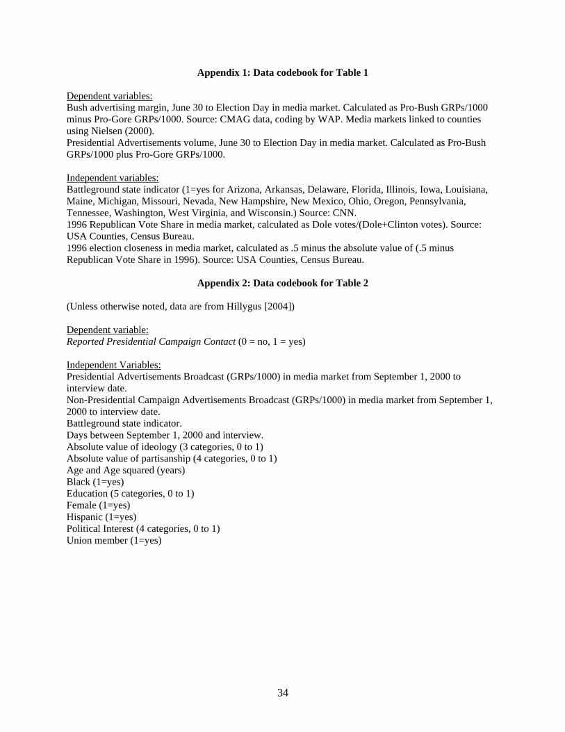
Appendix 1: Data codebook for Table 1 Dependent variables: Bush advertising margin, June 30 to Election Day in media market. Calculated as Pro-Bush GRPs/1000 minus Pro-Gore GRPs/1000. Source: CMAG data, coding by WAP. Media markets linked to counties using Nielsen (2000). Presidential Advertisements volume, June 30 to Election Day in media market. Calculated as Pro-Bush GRPs/1000 plus Pro-Gore GRPs/1000. Independent variables: Battleground state indicator (1=yes for Arizona, Arkansas, Delaware, Florida, Illinois, Iowa, Louisiana, Maine, Michigan, Missouri, Nevada, New Hampshire, New Mexico, Ohio, Oregon, Pennsylvania, Tennessee, Washington, West Virginia, and Wisconsin.) Source: CNN. 1996 Republican Vote Share in media market, calculated as Dole votes/(Dole+Clinton votes). Source: USA Counties, Census Bureau. 1996 election closeness in media market, calculated as .5 minus the absolute value of (.5 minus Republican Vote Share in 1996). Source: USA Counties, Census Bureau.

Appendix 2: Data codebook for Table 2

(Unless otherwise noted, data are from Hillygus [2004]) Dependent variable: Reported Presidential Campaign Contact (0 = no, 1 = yes) Independent Variables: Presidential Advertisements Broadcast (GRPs/1000) in media market from September 1, 2000 to interview date. Non-Presidential Campaign Advertisements Broadcast (GRPs/1000) in media market from September 1, 2000 to interview date. Battleground state indicator. Days between September 1, 2000 and interview. Absolute value of ideology (3 categories, 0 to 1) Absolute value of partisanship (4 categories, 0 to 1) Age and Age squared (years) Black (1=yes) Education (5 categories, 0 to 1) Female (1=yes) Hispanic (1=yes) Political Interest (4 categories, 0 to 1) Union member (1=yes)

34

Appendix 3: Data codebook for Tables 3-6 (Unless otherwise noted, data are from NAES.) Political Engagement Models Dependent Variables Interested in Presidential Campaign: (0 = not much, 1 = somewhat, 2 = very much) Intention to Vote: (0 = no, 1 = yes) Knowledge models Dependent Variables Respondents were asked to place candidates on following issues: Privatize Social Security (1 = Bush supports, Gore opposes, 0 = otherwise) Support School Vouchers (1 = Bush supports, Gore opposes, 0 = otherwise) Support Universal Health Care for Children (1 = Bush opposes, Gore supports, 0 = otherwise) Support Suing HMOs (1 = Bush opposes, Gore supports, 0 = otherwise) Favor Restricting Abortion (1 = Bush supports, Gore opposes, 0 = otherwise) Favor Death Penalty (1 = Bush and Gore supports, 0 = otherwise) Favor Handgun Licenses (1 = Bush opposes, Gore supports, 0 = otherwise) Placement of Bush and Gore on Ideology Scale (1 = Bush to right of Gore, 0 = otherwise) Bush or Gore Favors Biggest Tax Cut (1 = Bush favors, 0 = otherwise) Opionionation Models Dependent VariablesRespondents were asked to place candidates on following issues. If asked separately for two candidates, summed: Privatize Social Security (0 = don’t know, 1 = expressed belief) Support School Vouchers (0 = don’t know, 1 = expressed belief) Support Universal Health Care for Children (0 = don’t know, 1 = expressed belief) Support Suing HMOs (0 = don’t know, 1 = expressed belief) Favor Restricting Abortion (0 = don’t know, 1 = expressed belief) Favor Death Penalty (0 = don’t know, 1 = expressed belief) Favor Handgun Licenses (0 = don’t know, 1 = expressed belief) Placement of Bush and Gore on Ideology Scale (0 = don’t know, 1 = expressed belief) Bush or Gore Favors Biggest Tax Cut (0 = don’t know, 1 = expressed belief) Reinforcement Models Dependent VariablesRespondents were asked to express their positions on the following issues: Privatize Social Security (1 = Republicans support, Democrats oppose, 0 = otherwise) Support School Vouchers (1 = Republicans support, Democrats oppose, 0 = otherwise) Support Universal Health Care for Children (1 = Republicans oppose, Democrats support, 0 = otherwise) Support Suing HMOs (1 = Republicans oppose, Democrats support, 0 = otherwise) Favor Restricting Abortion (1 = Republicans support, Democrats oppose, 0 = otherwise) Favor Death Penalty (1 = Republicans support, Democrats oppose, 0 = otherwise) Favor Handgun Licenses (1 = Republicans oppose, Democrats support, 0 = otherwise) Vote Choice (1=Republicans support Bush, Democrats support Gore, 0 = otherwise)

35

Persuasion Models Dependent VariablesBush Favorability margin: Bush favorability (0 to 100 thermometer scale) minus Gore Favorability. Bush Likability margin: Bush Likes (Cumulative scale of four items asking respondents how well the following traits characterized Bush: caring, honest, inspiring, and knowledgeable. Scaled 0 to 1) minus Gore Likes Bush Vote Preference: (1= would vote for Bush if election held today, 0 = undecided, -1 = would vote for Gore if election held today) Independent VariablesFirst interview response to dependent variable Presidential Advertisement broadcast (GRPs/1000) in media market between interview dates. Non-Presidential Advertisements broadcast (GRPs/1000) in media market between interview dates. Absolute value of ideology (3 categories, 0 to 1) Ideology (-2 = very liberal, -1 = somewhat liberal, 0 = moderate, 1 = somewhat conservative, 2 = very conservative) Absolute value of party identification (4 categories, 0 to 1) Party identification (-3 = strong Democrat, -2 = weak Democrat, -1 = Independent leans Democrat, 0 = Pure Independent, 1 = Independent leans Republican, 2 = weak Republican, 3 = strong Republican) Attend Church (1 = yes) Union Member (1 = yes) Income (1 = less than 10K, 2 = 10K-15K, 3 = 15K-25K, 4 = 25K-35K, 5 = 35K-50K, 6 = 50-75K, 7 = 75K-100K, 8 = 100K-150K, 9 = 150K+) Employed (1 = yes) Education (1 = 8th grade or less, 2 = some high school, 3 = high school degree, 4 = vocational school, 5 = some college, 6 = associates degree, 7 = college degree, 8 = some graduate school, 9 = graduate degree) Hispanic (1 = yes) White (1 = yes) Female (1 = yes) Age and Age squared (in years) Competitive House Race (see Freedman, Franz, and Goldstein 2004) State fixed effects Week fixed effects Fixed effects for party conventions and debates

36

1A) Bush Advertising Margin (GRPs/1000) June 30 to November 7, 2000 by Media Market and State

Fixed Effects for State?-0.88

(0.590)4.66 * 5.33 ** 6.11 13.25 * 12.13 1.72 0.56

(2.546) (2.509) (4.244) (7.530) (7.376) (2.059) (4.847)-1.17 -1.86 -2.21 -6.09 * -5.55 0.30 0.94

(1.227) (1.228) (2.113) (3.615) (3.533) (0.958) (2.476)Observations 138 138 130 57 53 81 77R-squared 0.04 0.03 0.02 0.07 0.07 0.00 0.00

1B) Presidential Advertising Volume (GRPs/1000) June 30 to November 7, 2000 by Media Market and State

Fixed Effects for State?16.77 ***

(1.987)16.28 31.87 ** 29.47 25.05 70.79 13.93 10.61

(10.707) (14.510) (23.312) (37.925) (50.163) (9.068) (23.292)-0.76 -0.41 0.36 12.24 -7.93 0.22 1.74

(4.529) (6.021) (9.981) (16.234) (21.749) (3.858) (9.886)Observations 138 138 130 57 53 81 77R-squared 0.38 0.02 0.02 0.01 0.05 0.01 0.00

N/A N/A N/A N/A

(2)

No

(4)(3)

Republican Vote Share in 1996

Constant

Table 1: The 1996 Vote and Advertising in the 2000 Election

No Yes No Yes No Yes

Battleground State 2000

OLS coefficients with robust standard errors in parentheses in columns (1), (2), (4), and (6). See Appendix 1 for data sources and data coding. Fixed effects models include only states with multiple media markets. * denotes p<.10, ** denotes p<.05, *** denotes p<.01.

(6) (7)(1)All States Battleground States Non-Battleground States

(5)

N/A N/A

(5) (6) (7)All States Battleground States Non-Battleground States

(1) (2) (3) (4)

N/A N/A N/A

No No Yes No

Election Closeness 1996

Constant

OLS coefficients with robust standard errors in parentheses in columns (1), (2), (4), and (6). See Appendix 1 for data sources and data coding. Fixed effects models include only states with multiple media markets. * denotes p<.10, ** denotes p<.05, *** denotes p<.01.

Yes No Yes

Battleground State 2000 N/A N/A N/A

Fixed Effects for State?0.013 * 0.017 * 0.052 * -0.005

(0.0080) (0.0100) (0.0270) (0.0130)0.238 *

(0.1340)ObservationsLog-likelihood

Non-Battleground States


AllStates

(1) (2) (3)

Battleground States

Table 2: Reported Campaign Contact and Advertising Volume

Yes

N/A N/A

Presidential Advertising Volume (GRPs/1000) September 1 to November 7, 2000

No Yes

N/A

(4)

Yes

Probit coefficients with robust standard errors in parentheses, clustered by media zone. Coefficients for control variables and fixed effects (columns 2-4) not reported. See Appendix 2 for data sources, data coding, and full model specification. * denotes p<.10, ** denotes p<.05, *** denotes p<.01.

515-279.19

749-352.51-642.93-778.06

12641544

0.007 -0.028 **(0.010) (0.011)

N 1868 2051Log-likelihood -1444.49 -131.27Model Specification

Advertising Exposure (GRPs/1000)

Table 3: Advertising Exposure Effects on Campaign Interest and Vote Intention

Robust standard errors in parentheses, clustered by media zone. Advertising exposure is between first and second interview date. See Appendix 3 for data sources, data coding, and full model specification. * denotes p<.10, ** denotes p<.05, *** denotes p<.01.

Interest in Campaign Intention to Vote(1) (2)

Ordered Probit Probit

4A) Knowledge

0.039 ** 0.007 -0.028 * -0.008 0.018 0.017 ** -0.007 -0.011 0.019 * 0.000(0.017) (0.014) (0.014) (0.018) (0.030) (0.008) (0.014) (0.011) (0.010) (0.003)

N 1494 1559 1494 1494 1494 1559 1494 2817 2254 3701Log-likelihood -760.07 -801.40 -882.81 -840.65 -828.47 -825.33 -798.94 -1130.94 -1003.90 -5903.73Model Specification

4B) Opinionation

0.021 -0.019 -0.005 -0.007 -0.004 -0.002 0.001 0.009 -0.001 -0.002(0.019) (0.014) (0.024) (0.013) (0.051) (0.012) (0.018) (0.014) (0.012) (0.001)

N 1490 1551 1492 1492 856 1548 1493 2808 2252 3701Log-likelihood -725.66 -767.99 -874.73 -1065.54 -70.59 -789.40 -689.56 -473.01 -584.68 -8097.57Model Specification

4C) Reinforcement

0.025 *** 0.010 0.023 * -0.002 0.000 0.012 0.014 0.002 -0.031 **(0.007) (0.009) (0.012) (0.010) (0.008) (0.010) (0.010) (0.002) (0.013)

N 2375 3349 2375 2375 3349 2391 2375 3349 1964Log-likelihood -1161.58 -1460.55 -781.71 -918.72 -1280.10 -822.82 -931.08 -5958.91 -607.54Model Specification

(1) (2)

Probit Probit

Probit


Privatize Social Security

Support School Vouchers

Probit Probit Probit PoissonProbit Probit Probit Probit

Total ScaleFavor Restricting Abortion

Favor Death Penalty

Favor Gun Control Vote Choice


(8) (9)



Support Universal Health Care for Children

Support Suing HMOs

Probit Poisson


(1) (2) (3) (4) (5) (6) (7)

Bush or Gore Favors

Bigger Tax cutTotal Scale

Ordered Probit Ordered Probit Ordered Probit Ordered Probit Ordered Probit Ordered Probit Ordered Probit Ordered Probit

Favor Restricting Abortion

Favor Death Penalty

Favor Gun Control

Placement of Bush and Gore

on Ideology




Support Suing HMOs

(9) (10)


Support Suing HMOs

Favor Restricting Abortion

Favor Death Penalty

(8)

Probit

Placement of Bush and Gore

on Ideology

Bush or Gore Favors

Bigger Tax cutTotal Scale

Probit Probit Probit Probit

Favor Gun Control


(10)(3) (4) (5) (6) (7) (8) (9)

Probit

Table 4: Advertising Effects on Knowledge, Opinion Formation, and Reinforcement

(1) (2) (3) (4) (5) (6) (7)

Probit Poisson

4A) Knowledge

0.064 -0.082 -0.098 -0.069 -0.468 ***(0.102) (0.123) (0.203) (0.111) (0.122)

N 1494 1559 1494 1494 2254Log-likelihood -758.86 -801.15 -882.71 -840.19 -999.83Model Specification

4B) Opinionation

0.018 -0.141 -0.205 -0.260 * -0.206(0.167) (0.140) (0.145) (0.154) (0.128)

N 1490 1551 1492 1492 2252Log-likelihood -725.66 -767.64 -874.02 -1064.21 -584.17Model Specification

4C) Reinforcement

0.094 0.003 -0.125 0.133(0.190) (0.085) (0.101) (0.102)

N 2375 3349 2375 2375Log-likelihood -1161.50 -1460.54 -781.05 -918.14Model Specification

Table 5: Advertising Effects on Knowledge, Opinion Formation, and Reinforcement by Advertising Topic

(1) (2) (3) (4) (5)

Probit



(1)

Bush or Gore Favors

Bigger Tax cut


(3) (4) (5)

Probit

Bush or Gore Favors

Bigger Tax cut

Probit


Support Suing HMOs

Probit

Advertising Exposure on Topic (GRPs/1000)

(1) (2) (3) (4)

Ordered Probit Ordered Probit Ordered Probit Ordered Probit




Support Suing HMOs

Probit Probit


Probit




Support Suing HMOs


(2)

Probit Probit

Probit

0.499 0.002 0.157 ***(0.378) (0.011) (0.042)

0.157 0.002 0.184 ***(0.381) (0.011) (0.048)-0.816 * -0.002 -0.132 ***

(0.425) (0.011) (0.040)N 3541 3541 3232 3232 2142 2142Log-likelihood 0.75 0.75 0.76 0.76 -896.13 -896.11Model Specification

Table 6: The Persuasive Effects of Advertising

Bush Advertising(GRPs/1000)

Bush Advertising Margin (GRPs/1000)

(4) (5) (6)(2)

Bush Vote Preference(Bush, undecided, Gore)

(3)(1)


Ordered Probit Ordered ProbitOLSOLS OLS

Bush Favorability Margin(Bush minus Gore Favorability)

Bush Likability Margin(Bush minus Gore Likability)

OLS

Gore Advertising(GRPs/1000)

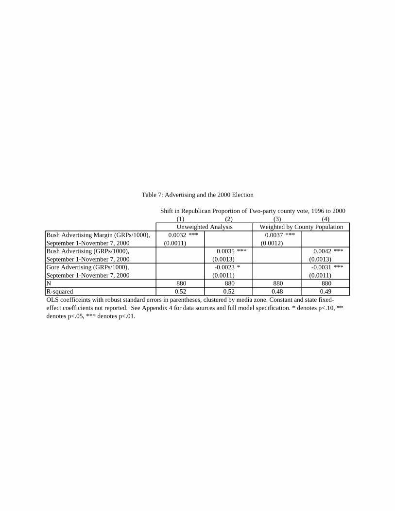
0.0032 *** 0.0037 ***(0.0011) (0.0012)

0.0035 *** 0.0042 ***(0.0013) (0.0013)-0.0023 * -0.0031 ***

(0.0011) (0.0011)N 880 880 880 880R-squared 0.52 0.52 0.48 0.49

(3)(1)

OLS coefficeints with robust standard errors in parentheses, clustered by media zone. Constant and state fixed-effect coefficients not reported. See Appendix 4 for data sources and full model specification. * denotes p<.10, ** denotes p<.05, *** denotes p<.01.

Table 7: Advertising and the 2000 Election

Bush Advertising (GRPs/1000), September 1-November 7, 2000

Bush Advertising Margin (GRPs/1000), September 1-November 7, 2000

(4)(2)Shift in Republican Proportion of Two-party county vote, 1996 to 2000

Unweighted Analysis Weighted by County Population

Gore Advertising (GRPs/1000), September 1-November 7, 2000

State Winner

Winner's Percentage,2-party vote

Winner'smargin,votes

Bush GRPs/1000 in State

Bush spending in state

Gore GRPs/1000 in State

Gore spending in state

Votesin largest

media market

GRPs/1000 Necessary to Induce Tie

Estimated CostPer

GRPs/1000

Total Cost Necessary to Induce Tie

Florida Bush 50.00% 537 70.5 $11,300,000 43.5 $7,343,064 1,505,471 0.0 $170,840 $8,235New Mexico Gore 50.03% 366 9.9 $1,158,680 9.2 $1,081,477 514,477 0.1 $117,059 $11,254Wisconsin Gore 50.12% 5,708 30.3 $3,568,025 33.0 $3,510,116 1,068,467 0.7 $126,510 $91,330Iowa Gore 50.16% 4,144 14.0 $719,120 14.3 $716,661 467,204 1.2 $48,995 $58,727Oregon Gore 50.24% 6,765 22.4 $2,513,376 21.5 $2,518,812 1,002,851 0.9 $150,092 $136,823New Hampshire Bush 50.67% 7,211 11.9 $1,887,351 6.8 $960,284 473,201 2.1 $632,294 $1,302,078Minnesota Gore 51.29% 58,607 4.2 $1,202,573 3.2 $916,477 1,930,306 4.1 $286,897 $1,177,112Missouri Bush 51.71% 78,786 34.4 $3,742,470 42.4 $4,759,145 826,637 12.9 $154,767 $1,993,340Ohio Bush 51.82% 165,019 51.5 $5,977,748 53.0 $6,445,223 1,617,435 13.8 $206,524 $2,847,380Nevada Bush 51.86% 21,597 8.6 $1,607,559 7.0 $1,268,924 396,335 7.4 $184,170 $1,356,185Tennessee Bush 51.96% 80,229 15.8 $1,233,890 11.6 $933,488 751,472 14.4 $96,351 $1,390,096Pennsylvania Gore 52.15% 204,840 44.3 $9,206,702 49.6 $10,200,000 1,948,796 14.2 $448,662 $6,372,881Maine Gore 52.75% 33,335 10.2 $797,250 5.9 $416,159 446,841 10.1 $75,268 $758,797Michigan Gore 52.63% 217,279 58.3 $7,309,387 64.6 $7,856,574 2,090,977 14.0 $282,589 $3,968,189Arkansas Bush 52.80% 50,172 17.8 $1,149,427 15.7 $991,017 476,177 14.2 $61,342 $873,418Washington Gore 52.94% 138,788 32.2 $5,513,252 31.8 $5,524,718 1,850,598 10.1 $299,555 $3,035,882

Table 8: Campaign Spending Necessary to Swing the 16 Closest States in 2000

Notes: Votes in media market calculated from 2000 election returns. Advertising data and expenditures from CMAG, coded by WAP. GRPs necessary to induce tie calculated from assumption that each GRPs/1000 in advertising increases candidate's proportion of vote by .0037 and decreases opponents proportion by .0037 (See Table 7). Estimated cost calculated from observed cost per GRP for presidential advertising, September 1, 2000 to Election Day. See Appendix 4 for data sources.

Full Model Results Appendix for Tables 2, 3, and 6 In order to save space, this manuscript includes several tables where we report only coefficients for the effects of advertising on our dependent variables of interest. Here we include the full results for the models shown in Tables 2, 3, and 6.

Fixed Effects for State?0.013 * 0.017 * 0.052 * -0.005

(0.0080) (0.0100) (0.0270) (0.0130)0.238 *

(0.1340)0.121 ** 0.084 0.069 0.127

(0.0590) (0.0680) (0.1120) (0.0820)-0.135 -0.071 -0.275 0.079

(0.1370) (0.1320) (0.2540) (0.1650)-0.316 -0.315 -1.329 ** -0.088

(0.2090) (0.2210) (0.5810) (0.1850)0.490 *** 0.462 *** 0.839 *** 0.250

(0.1440) (0.1600) (0.2790) (0.1860)0.016 0.017 0.036 * 0.001

(0.0120) (0.0130) (0.0210) (0.0150)0.000 0.000 0.000 0.000

0.0000 0.0000 0.0000 0.00000.158 0.186 * -0.091 0.324 ***

(0.1110) (0.1070) (0.1630) (0.1230)0.366 *** 0.360 *** 0.552 *** 0.227 **

(0.1020) (0.1080) (0.1960) (0.1150)0.203 ** 0.255 ** 0.438 ** 0.161

(0.0890) (0.1050) (0.2050) (0.1140)

-2.137 *** -2.028 *** -3.572 *** -1.440 ***(0.3310) (0.3550) (0.9470) (0.3640)

ObservationsLog-likelihoodProbit coefficients with robust standard errors in parentheses, clustered by media zone. Coefficients for control variables and fixed effects (columns 2-4) not reported. See Appendix 2 for data sources, data coding, and full model specification. * denotes p<.10, ** denotes p<.05, *** denotes p<.01.

515-279.19

749-352.51-642.93-778.06

12641544

Full model results for Table 2: Reported Campaign Contact and Advertising Volume

Yes

N/A N/A

Presidential Advertising Volume (GRPs/1000) September 1 to November 7, 2000

No Yes

N/A

(4)

Yes

Non-Battleground States


AllStates

(1) (2) (3)

Battleground States

N/A Not Reportedto save space

Not Reportedto save space


Female (1=yes)

Black (1=yes)

Hispanic (1=yes)

Education

Union member (1=yes)

State indicator variables

Constant

Age

Age squared

Absolute value of ideology score

Absolute value of partisanship score

0.007 -0.028 **(0.010) (0.011)-2.265 ***

(0.127)-1.259 ***

(0.079)3.432 ***

(0.224)0.000 0.000

(0.004) (0.017)0.002 0.212

(0.034) (0.170)0.086 ** 0.128 *

(0.037) (0.070)0.188 0.154

(0.130) (0.253)-0.032 -0.338

(0.088) (0.228)0.044 ** 0.116 **

(0.021) (0.048)-0.082 -0.038

(0.078) (0.285)0.051 *** 0.020

(0.014) (0.042)0.073 -0.782

(0.141) (0.557)-0.009 0.165

(0.063) (0.182)-0.109 * 0.136

(0.061) (0.173)0.000 0.054 **

(0.013) (0.022)0.000 -0.001 **

0.000 0.000-0.183 * 0.731

(0.095) (0.497)

N 1868 2051Log-likelihood -1444.49 -131.27Model Specification


Full model results for Table 3: Advertising Exposure Effects on Campaign Interest and Vote Intention


Interest in Campaign Intention to Vote(1) (2)

Ordered Probit Probit

Lagged campaign Interest=0

Absolute value of partisanship score

Attend Church (1=yes)


Lagged campaign Interest=.5

Lagged vote intention

Other advertising (GRPs/1000)

Absolute value of ideology score

Week of reinterview indicator variables

Significant campaign event indicators

Female (1=yes)

Age

Age squared

Income

Competitive House District Indicator


Not Reportedto save spaceState indicator variables

Employed (1=yes)

Education

Hispanic (1=yes)

White (1=yes)

Not Reportedto save spaceNot Reportedto save space

Not Reportedto save spaceNot Reportedto save space

0.499 0.002 0.157 ***(0.378) (0.011) (0.042)

0.157 0.002 0.184 ***(0.381) (0.011) (0.048)-0.816 * -0.002 -0.132 ***

(0.425) (0.011) (0.040)0.660 *** 0.660 ***

(0.021) (0.021)-0.723 *** -0.723 ***

(0.027) (0.027)0.772 *** 0.772 ***

(0.026) (0.026)-0.756 *** -0.756 ***

(0.032) (0.032)1.221 *** 1.221 ***

(0.102) (0.102)-1.146 *** -1.146 ***

(0.093) (0.093)-0.323 ** 0.000 0.025 *

(0.149) (0.003) (0.014)0.101 0.100 0.000 0.000 -0.004 -0.005

(0.062) (0.062) (0.002) (0.002) (0.006) (0.006)3.408 *** 3.408 *** 0.076 *** 0.076 *** 0.127 ** 0.127 **

(0.946) (0.946) (0.027) (0.027) (0.063) (0.063)4.304 *** 4.304 *** 0.143 *** 0.143 *** 0.243 *** 0.243 ***

(0.544) (0.544) (0.013) (0.013) (0.027) (0.027)2.986 * 2.984 * 0.029 0.029 0.366 *** 0.366 ***

(1.562) (1.562) (0.048) (0.048) (0.125) (0.125)0.245 0.243 0.059 0.059 -0.051 -0.051

(1.653) (1.653) (0.050) (0.050) (0.134) (0.134)-0.322 -0.321 -0.001 -0.001 0.014 0.014

(0.313) (0.313) (0.010) (0.010) (0.024) (0.024)0.702 0.701 -0.021 -0.021 0.100 0.100

(1.567) (1.567) (0.052) (0.052) (0.114) (0.114)0.087 0.087 0.012 0.012 -0.031 ** -0.031 **

(0.264) (0.264) (0.007) (0.007) (0.016) (0.016)-0.056 -0.055 0.004 0.004 0.074 0.074

(1.690) (1.690) (0.061) (0.061) (0.164) (0.164)4.813 ** 4.815 ** 0.184 *** 0.184 *** 0.401 *** 0.401 ***

(1.984) (1.984) (0.042) (0.042) (0.128) (0.128)-2.609 ** -2.608 ** -0.057 ** -0.057 ** -0.262 *** -0.262 ***

(1.184) (1.184) (0.028) (0.028) (0.070) (0.070)0.113 0.113 0.004 0.004 0.011 0.011

(0.147) (0.147) (0.005) (0.005) (0.010) (0.010)-0.001 -0.001 0.000 0.000 0.000 0.000

(0.002) (0.002) 0.000 0.000 0.000 0.000-0.865 -0.867 0.062 0.062 -0.135 -0.135

(2.251) (2.250) (0.091) (0.091) (0.168) (0.168)

N 3541 3541 3232 3232 2142 2142Log-likelihood 0.75 0.75 0.76 0.76 -896.13 -896.11Model Specification

Bush Favorability Margin(Bush minus Gore Favorability)

Bush Likability Margin(Bush minus Gore Likability)

OLS

Gore Advertising(GRPs/1000)








Ordered Probit Ordered ProbitOLSOLS OLS

Full model results for Table 6: The Persuasive Effects of Advertising

Bush Advertising(GRPs/1000)

Bush Advertising Margin (GRPs/1000)

(4) (5) (6)(2)

Bush Vote Preference(Bush, undecided, Gore)

(3)(1)













Lagged Bush Favorability

Lagged Gore Favorability

Lagged Bush Likes

Lagged Gore Likes

Lagged Bush Vote (1=yes)

Lagged Gore Vote (1=yes)

Total Presidential Advertising (GRPs/1000)

Other advertising (GRPs/1000)

Ideology score

Partisanship score

Attend Church (1=yes)


Income

Employed (1=yes)

Education

Hispanic (1=yes)

White (1=yes)

Female (1=yes)

Age

Age squared

Competitive House District Indicator

State indicator variables

Week of reinterview indicator variablesSignificant campaign event indicators

uncovering the persuasive effects of presidential advertising · yet the finding that campaign...

Documents