uncovering the distribution of motoristsâ€™ preferences for travel

UNCOVERING THE DISTRIBUTION OF MOTORISTS’ PREFERENCES FOR

TRAVEL TIME AND RELIABILITY

by Kenneth A. Small, Clifford Winston, and Jia Yan

January 19, 2005

forthcoming, Econometrica

Abstract

We apply recent econometric advances to study the distribution of commuters’ preferences for speedy and reliable highway travel. Our analysis applies mixed logit to combined revealed and stated preference data on commuter choices of whether to pay a toll for congestion-free express travel. We find that motorists exhibit high values of travel time and reliability and substantial heterogeneity in those values. We suggest that road pricing policies designed to cater to such varying preferences can improve efficiency and reduce the disparity of welfare impacts compared with recent pricing experiments. Keywords: mixed logit, stated preference, congestion pricing, product differentiation, value of time Kenneth A. Small* Department of Economics University of California Irvine, CA 92697-5100 USA [email protected]

Clifford Winston Brookings Institution 1775 Mass. Ave., N.W. Washington, DC 20036 USA [email protected]

Jia Yan Department of Logistics Hong Kong Polytechnic University Hung Hom, Kowloon Hong Kong [email protected]

*Corresponding author

Acknowledgment

The authors are grateful to the Brookings Center on Urban and Metropolitan Policy and the

University of California Transportation Center for financial support. We thank Edward Sullivan for

access to data collected by California Polytechnic State University at San Luis Obispo, with

financial support from the California Department of Transportation and the U.S. Federal Highway

Administration’s Value Pricing Demonstration Program. We also are grateful for comments from

David Brownstone, Jerry Hausman, Charles Lave, Steven Morrison, and Randy Pozdena; from

participants in seminars at UC Irvine, Northwestern University, the American Economic

Association, and the University of Maryland at College Park; and from the referees and a co-editor

of this journal.

Small, Winston, & Yan Preferences for Travel Time & Reliability

1

1. Introduction

Efficient pricing is rarely used to ameliorate highway congestion, probably because of its

immediate adverse impact on a representative traveler. Recent experiments in the United States

have therefore tried to make pricing more appealing by giving motorists the option to travel free

on regular lanes or to pay for congestion-free travel on express lanes—a policy sometimes called

“value pricing.”

Theory suggests that the benefits of differentiated road pricing depend critically on the

cross-sectional variation in motorists’ preferences for speedy and reliable travel (Small and Yan

(2001) and Verhoef and Small (2004)). However, econometric evidence on travelers’ preference

variation is quite limited. Value-of-time studies often capture observed heterogeneity by

allowing estimated values to depend on the wage rate, income, and other factors (Small and

Winston (1999), Wardman (2001)). But the previous studies have limitations. Those based solely

on data describing actual choices, i.e., revealed preference (RP) data, have been hampered by

collinearity among cost and travel-time variables; consequently they rarely have accounted for

reliability (i.e., the predictability of travel time) and they have not accounted for heterogeneity in

cost or travel-time elasticities arising from unobserved sources. Calfee, Winston, and Stempski

(2001) and Hensher (2001) measure the extent of unobserved heterogeneity using stated

preference (SP) data describing hypothetical responses; but SP data are tainted by doubt whether

behavior exhibited in hypothetical situations applies to actual choices.

In this paper, we estimate the distribution of values of travel time savings and reliability,

allowing for both observed and unobserved heterogeneity. We do so by analyzing a sample of

motorists who can participate in a value-pricing experiment in the Los Angeles area. These

motorists face considerable variation in tolls and other factors. We enrich that variation by


2

combining RP data from actual choices with SP data from hypothetical situations that are aligned

with the pricing experiment. Combining the two types of data enables us to obtain statistically

precise estimates while still allowing for possible differences between actual and hypothetical

behavior.

We find that commuters differ substantially in how they value travel time and reliability.

We find also that the average valuation of both is quite high, and is considerably higher when

measured in real as opposed to hypothetical scenarios. We suggest that these findings offer

possibilities of designing differentiated pricing schemes that are more efficient and that create

smaller disparities among users than do current value-pricing experiments.

2. Empirical Setting and Data Overview1

The route of interest is California State Route 91 (SR91) in greater Los Angeles. A ten-mile

portion of the route in Orange County, used heavily by long-distance commuters, includes four

regular freeway lanes (91F) and two express lanes (91X) in each direction. Motorists who wish to

use the express lanes must set up a financial account and carry an electronic transponder in order to

pay a toll, which varies hourly according to a preset schedule.

We combine three samples of people traveling on this corridor, based on surveys taken over

a ten-month period in 1999 and 2000. The first is a telephone RP survey conducted by researchers at

California Polytechnic State University at San Luis Obispo (Cal Poly) with our participation

(Sullivan et al. (2000)). It includes both commuting and other trips. The second and third samples

are from a two-stage mail survey collected by us through the Brookings Institution. It used the

database of a market research firm, along with a pre-screening survey, to obtain a random sample of

1 Additional details of our data collection and methodological procedures are contained in our appendix on the Econometrica web site.


3

potential rush-hour commuters on the corridor. The first stage of the Brookings survey collected RP

data on actual trips. The second stage presented eight SP scenarios where the respondent could

choose between two otherwise identical routes with specified hypothetical tolls, travel times, and

probabilities of delay. Our econometric design allows us to treat each RP observation and each of

the multiple SP observations for any given individual as separate observations with appropriate

error correlations. The final sample consisted of RP data on 522 distinct individuals and SP data

totaling 633 observations on 81 distinct individuals (55 of whom also answered the RP questions.)

Table 1 presents some summary statistics. The Cal Poly and Brookings RP samples have

nearly identical shares of people using the express lanes. The Brookings samples appear to

represent well the population characteristics of the SR91 catchment area, tracking Census

information for the two relevant counties except for household income — which, naturally, is higher

for our respondents because most of them are commuters. The Cal Poly sample has higher

household incomes and shorter trip distances than the Brookings samples, evidently being drawn

from a narrower and more affluent geographical area; we therefore condition our choice model

on these two variables.

3. Econometric Framework

Our basic model specifies the choice between express and regular lanes as conditional on

related choices including residential location, travel mode (car or public transport), time of day, and

car occupancy. The choice is also conditional on transponder acquisition for SP respondents, but is

unconditional on transponder acquisition for RP respondents.2 Integrating all these decisions with

2 SP respondents were instructed to assume they had a transponder, so if they followed this instruction their lane choice is conditional on having a transponder. If instead they took as given their actual transponder status, then we could have selection bias to the extent that their actual transponder status is correlated with unobserved preferences for the express lane. We assume that any selection bias arising in this way is controlled for by specifying a random constant for lane choice by SP respondents, as we describe in this section. We found that results were not affected by adding a control variable describing the transponder status of the SP respondent’s actual commute.


4

lane choice would enrich the analysis, but would unlikely affect the results of interest here. For

instance, mode choice is unimportant because public transportation has a very small share of

travelers in this corridor. Location choice is typically a long-run decision and the express lanes had

been open only a few years. We discuss later the effects of endogenous choices of car occupancy,

transponder acquisition, and time of day; the latter is the most critical because our ability to identify

the effects of cost, time, and reliability depends on their variation throughout the rush-hour period.

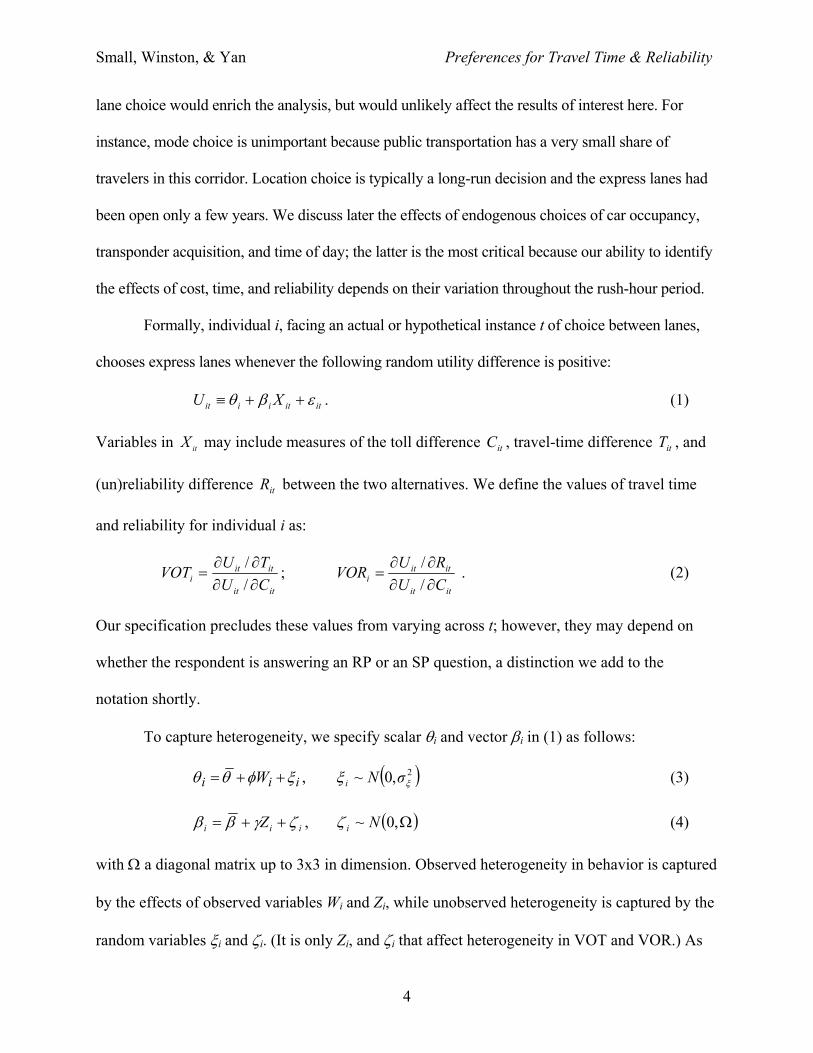
Formally, individual i, facing an actual or hypothetical instance t of choice between lanes,

chooses express lanes whenever the following random utility difference is positive:

ititiiit XU εβθ ++≡ . (1)

Variables in itX may include measures of the toll difference itC , travel-time difference itT , and

(un)reliability difference itR between the two alternatives. We define the values of travel time

and reliability for individual i as:

itit

ititi CU

TUVOT∂∂∂∂

=// ;

itit

ititi CU

RUVOR∂∂∂∂

=// . (2)

Our specification precludes these values from varying across t; however, they may depend on

whether the respondent is answering an RP or an SP question, a distinction we add to the

notation shortly.

To capture heterogeneity, we specify scalar θi and vector βi in (1) as follows:

iii W ξφθθ ++= , ( )2,0~ ξξ σNi (3)

iii Z ζγββ ++= , ( )Ω,0~ Niζ (4)

with Ω a diagonal matrix up to 3x3 in dimension. Observed heterogeneity in behavior is captured

by the effects of observed variables Wi and Zi, while unobserved heterogeneity is captured by the

random variables ξi and ζi. (It is only Zi, and ζi that affect heterogeneity in VOT and VOR.) As


5

indicated, we specified the components of ζi as normally distributed; we also tried log-normal

and truncated normal distributions but similar to others (Train (2001)) we were unable to obtain

convergence.

We denote our three data subsets by superscripts BR (Brookings RP), BS (Brookings SP),

and C (Cal Poly). All the RP observations have a single choice instance t, so we can write

BRi

BRit εε = and C

iCit ηε = .3 We further split BR

iε and BSitε into components (denoted by ν and η),

with one part in common, to allow for correlation between RP and SP observations of the same

individual (determined by a multiplier ρ) and among multiple SP observations from one

individual (determined by the relative variances of BSiν and BS

itη ). These assumptions transform

(1) into the following system after substituting (3) for θi:

BRi

BRi

BRi

BRi

BRi

BRBRBRi XWU ηνβφθ ++++≡ (5a)

BSit

BSi

BRi

BSit

BSi

BSi

BSBSBSit XWU ηξρνβφθ +++++≡ (5b)

Ci

Ci

Ci

Ci

CCCi XWU ηβφθ +++≡ (5c)

where random parameters βi are as in (4) and ( )1,0~ NBRiν . We have set BR

iξ = Ciξ =0 in (3)

because, with only one observation per individual, these two random variables are redundant

with BRiη and C

iη . We assume that BRiη , BS

itη , and Ciη have independent logistic distributions,

yielding the familiar logit formula for the choice probability conditional on other random

parameters; our treatment of unobserved heterogeneity is therefore an example of the mixed logit

model described by McFadden and Train (2000) and Train (2003).

3 The Brookings RP sample actually contains information for all commuting trips made within the survey week, which could be treated as separate observations. However, 87 percent of the respondents made the same choice every day and nearly all of the others varied on only one day. So we simplify, with little information loss, by creating a binary response variable equal to one if the respondent chose the express lanes for half or more of the days reported. We tried variants of this response variable with virtually no changes in results.


6

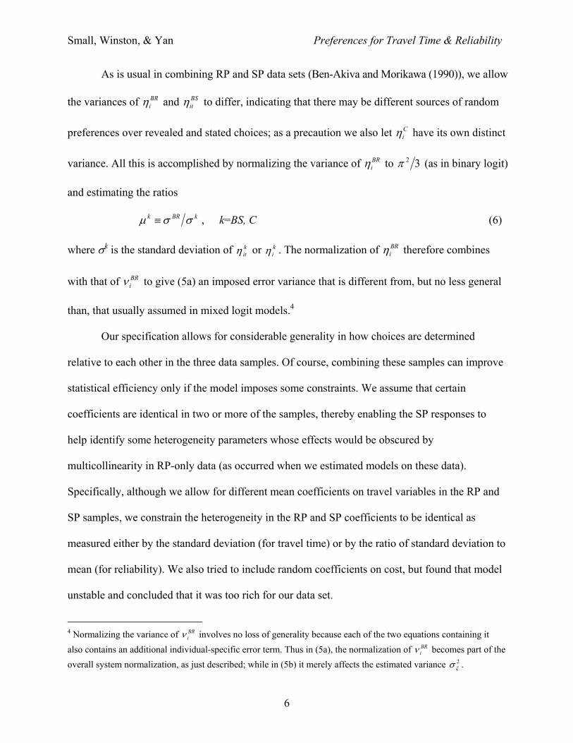
As is usual in combining RP and SP data sets (Ben-Akiva and Morikawa (1990)), we allow

the variances of BRiη and BS

itη to differ, indicating that there may be different sources of random

preferences over revealed and stated choices; as a precaution we also let Ciη have its own distinct

variance. All this is accomplished by normalizing the variance of BRiη to 32π (as in binary logit)

and estimating the ratios

kBRk σσµ ≡ , k=BS, C (6)

where σk is the standard deviation of kitη or k

iη . The normalization of BRiη therefore combines

with that of BRiν to give (5a) an imposed error variance that is different from, but no less general

than, that usually assumed in mixed logit models.4

Our specification allows for considerable generality in how choices are determined

relative to each other in the three data samples. Of course, combining these samples can improve

statistical efficiency only if the model imposes some constraints. We assume that certain

coefficients are identical in two or more of the samples, thereby enabling the SP responses to

help identify some heterogeneity parameters whose effects would be obscured by

multicollinearity in RP-only data (as occurred when we estimated models on these data).

Specifically, although we allow for different mean coefficients on travel variables in the RP and

SP samples, we constrain the heterogeneity in the RP and SP coefficients to be identical as

measured either by the standard deviation (for travel time) or by the ratio of standard deviation to

mean (for reliability). We also tried to include random coefficients on cost, but found that model

unstable and concluded that it was too rich for our data set.

4 Normalizing the variance of BR

iν involves no loss of generality because each of the two equations containing it also contains an additional individual-specific error term. Thus in (5a), the normalization of BR

iν becomes part of the overall system normalization, as just described; while in (5b) it merely affects the estimated variance 2

ξσ .


7

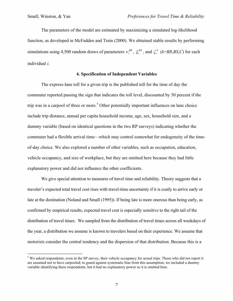
The parameters of the model are estimated by maximizing a simulated log-likelihood

function, as developed in McFadden and Train (2000). We obtained stable results by performing

simulations using 4,500 random draws of parameters BRiν , BS

iξ , and kiζ (k=BR,BS,C) for each

individual i.

4. Specification of Independent Variables

The express-lane toll for a given trip is the published toll for the time of day the

commuter reported passing the sign that indicates the toll level, discounted by 50 percent if the

trip was in a carpool of three or more.5 Other potentially important influences on lane choice

include trip distance, annual per capita household income, age, sex, household size, and a

dummy variable (based on identical questions in the two RP surveys) indicating whether the

commuter had a flexible arrival time—which may control somewhat for endogeneity of the time-

of-day choice. We also explored a number of other variables, such as occupation, education,

vehicle occupancy, and size of workplace, but they are omitted here because they had little

explanatory power and did not influence the other coefficients.

We give special attention to measures of travel time and reliability. Theory suggests that a

traveler’s expected total travel cost rises with travel-time uncertainty if it is costly to arrive early or

late at the destination (Noland and Small (1995)). If being late is more onerous than being early, as

confirmed by empirical results, expected travel cost is especially sensitive to the right tail of the

distribution of travel times. We sampled from the distribution of travel times across all weekdays of

the year, a distribution we assume is known to travelers based on their experience. We assume that

motorists consider the central tendency and the dispersion of that distribution. Because this is a

5 We asked respondents, even in the SP survey, their vehicle occupancy for actual trips. Those who did not report it are assumed not to have carpooled; to guard against systematic bias from this assumption, we included a dummy variable identifying these respondents, but it had no explanatory power so it is omitted here.


8

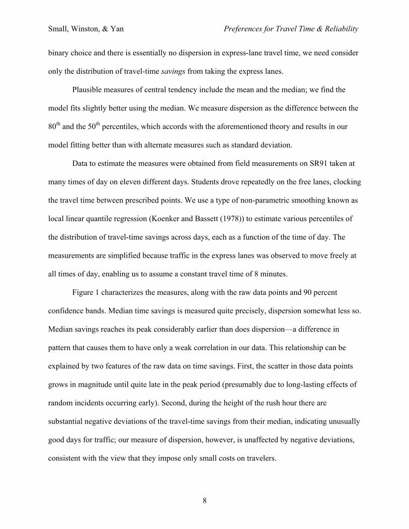
binary choice and there is essentially no dispersion in express-lane travel time, we need consider

only the distribution of travel-time savings from taking the express lanes.

Plausible measures of central tendency include the mean and the median; we find the

model fits slightly better using the median. We measure dispersion as the difference between the

80th and the 50th percentiles, which accords with the aforementioned theory and results in our

model fitting better than with alternate measures such as standard deviation.

Data to estimate the measures were obtained from field measurements on SR91 taken at

many times of day on eleven different days. Students drove repeatedly on the free lanes, clocking

the travel time between prescribed points. We use a type of non-parametric smoothing known as

local linear quantile regression (Koenker and Bassett (1978)) to estimate various percentiles of

the distribution of travel-time savings across days, each as a function of the time of day. The

measurements are simplified because traffic in the express lanes was observed to move freely at

all times of day, enabling us to assume a constant travel time of 8 minutes.

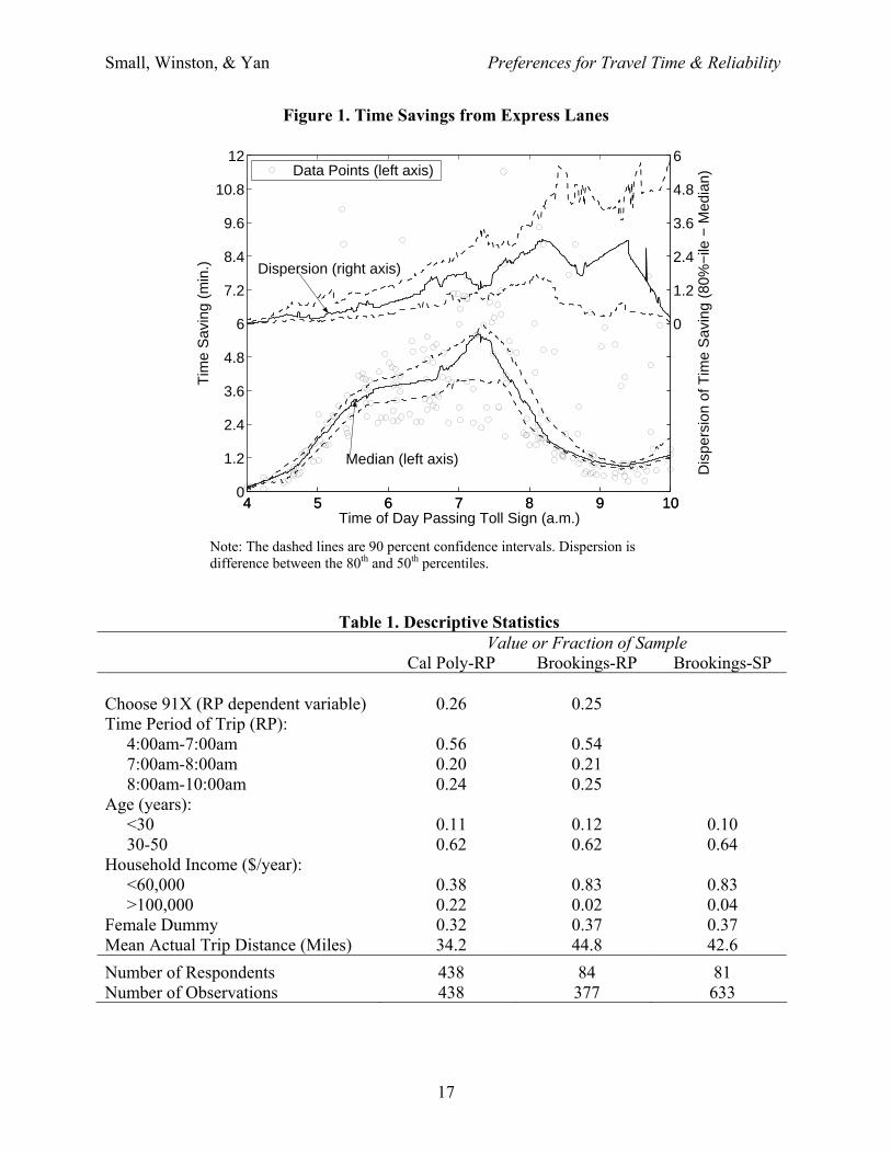
Figure 1 characterizes the measures, along with the raw data points and 90 percent

confidence bands. Median time savings is measured quite precisely, dispersion somewhat less so.

Median savings reaches its peak considerably earlier than does dispersion—a difference in

pattern that causes them to have only a weak correlation in our data. This relationship can be

explained by two features of the raw data on time savings. First, the scatter in those data points

grows in magnitude until quite late in the peak period (presumably due to long-lasting effects of

random incidents occurring early). Second, during the height of the rush hour there are

substantial negative deviations of the travel-time savings from their median, indicating unusually

good days for traffic; our measure of dispersion, however, is unaffected by negative deviations,

consistent with the view that they impose only small costs on travelers.


9

Most SP variables correspond in definition to the RP variables. An exception is the

measure of unreliability. We did not think survey respondents would understand statements

about percentiles of a probability distribution, so in our SP scenarios we specified the frequency

of being delayed 10 minutes or more, which we convert into a probability for analysis.

5. Estimation Results

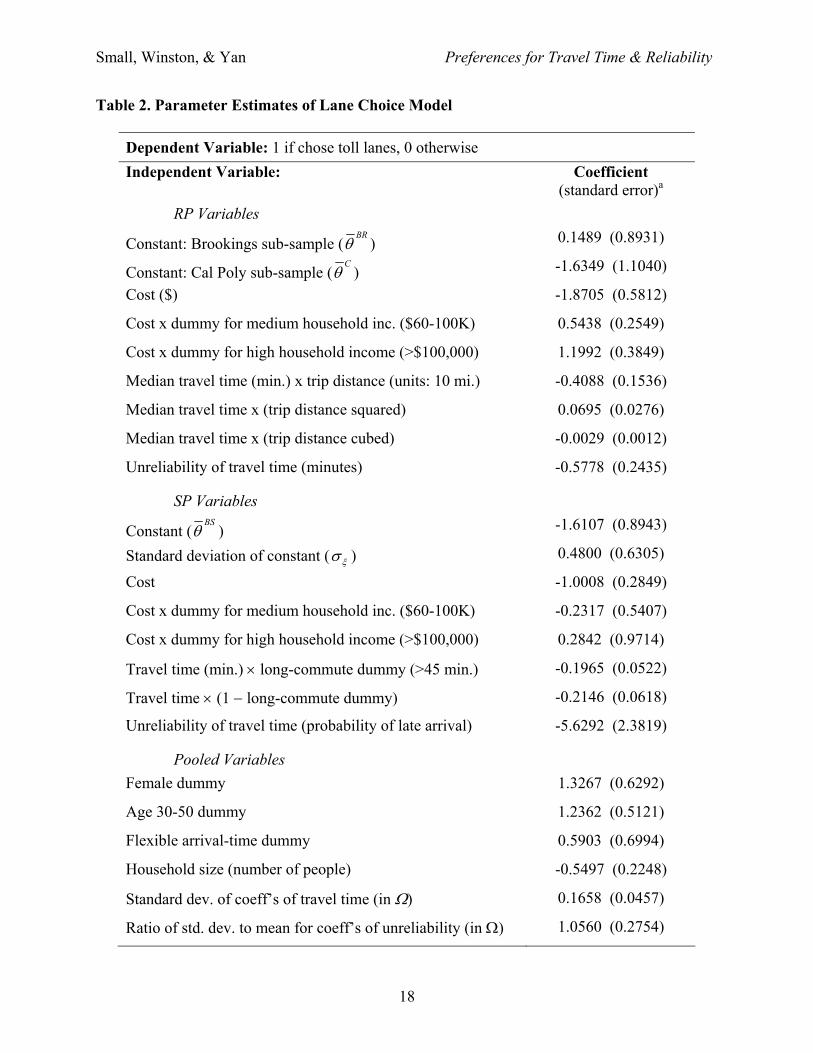
Estimation results are presented in table 2. Most influences are statistically significant

and have the expected sign. Both the RP and SP coefficients indicate that commuters are deterred

from the express lanes by a higher toll and are deterred from the free lanes by longer median

travel times and greater unreliability—findings that hold throughout the range of the interaction

variables.

The implied elasticities of express-lane usage with respect to toll, travel-time savings,

and unreliability are shown at the bottom of the table. All three variables have a substantial

impact on the decision to use the express lanes. To better understand the price elasticity of -1.59,

consider that the private operator of the express lanes maximizes profit by setting a price so that

marginal revenue equals short-run marginal cost, which on the express lanes is near zero. But the

marginal revenue is less than that given by the usual formula involving the demand elasticity,

because each additional car using the express lanes reduces the attraction of those lanes to others

by relieving congestion on the regular lanes. If that congestion is severe, the elasticity of demand

must be substantially greater than one in magnitude in order to produce marginal revenue near

zero as required for a profit-maximizing equilibrium.

Observed heterogeneity is captured by interactions between cost and income, and

between time and three powers of trip distance—these are the variables Z in equation (4).

Consistent with expectations, motorists with higher incomes are less responsive to the toll. The


10

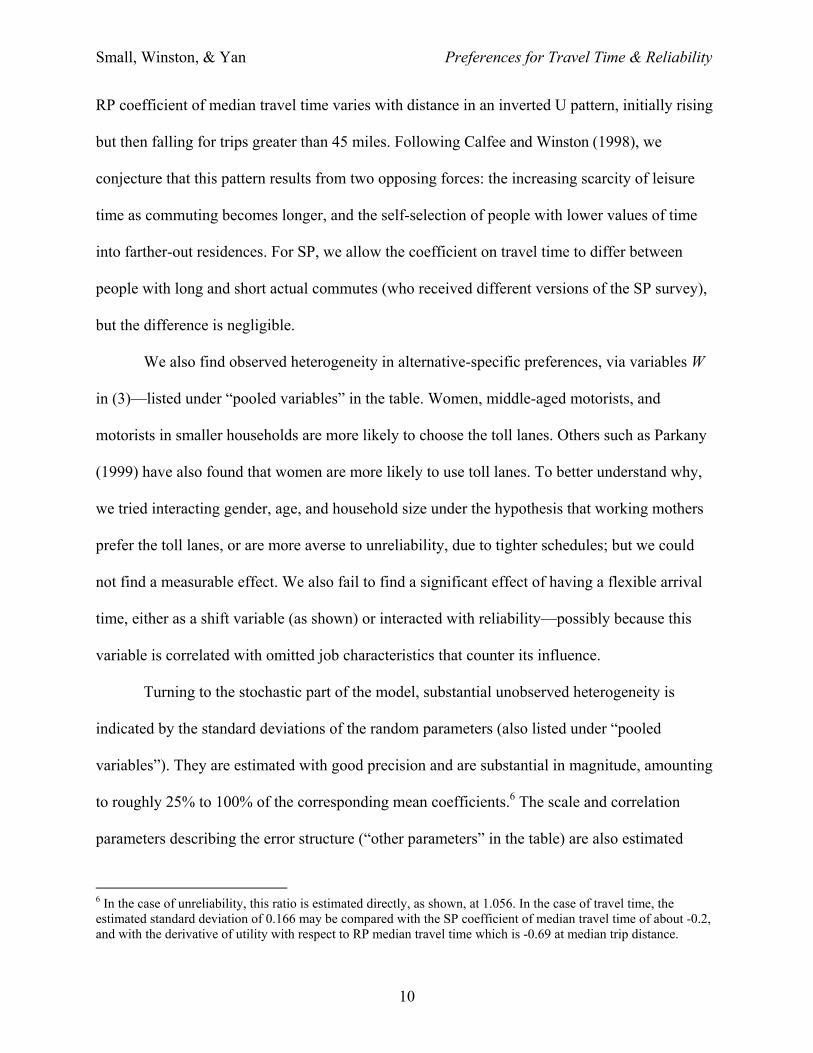
RP coefficient of median travel time varies with distance in an inverted U pattern, initially rising

but then falling for trips greater than 45 miles. Following Calfee and Winston (1998), we

conjecture that this pattern results from two opposing forces: the increasing scarcity of leisure

time as commuting becomes longer, and the self-selection of people with lower values of time

into farther-out residences. For SP, we allow the coefficient on travel time to differ between

people with long and short actual commutes (who received different versions of the SP survey),

but the difference is negligible.

We also find observed heterogeneity in alternative-specific preferences, via variables W

in (3)—listed under “pooled variables” in the table. Women, middle-aged motorists, and

motorists in smaller households are more likely to choose the toll lanes. Others such as Parkany

(1999) have also found that women are more likely to use toll lanes. To better understand why,

we tried interacting gender, age, and household size under the hypothesis that working mothers

prefer the toll lanes, or are more averse to unreliability, due to tighter schedules; but we could

not find a measurable effect. We also fail to find a significant effect of having a flexible arrival

time, either as a shift variable (as shown) or interacted with reliability—possibly because this

variable is correlated with omitted job characteristics that counter its influence.

Turning to the stochastic part of the model, substantial unobserved heterogeneity is

indicated by the standard deviations of the random parameters (also listed under “pooled

variables”). They are estimated with good precision and are substantial in magnitude, amounting

to roughly 25% to 100% of the corresponding mean coefficients.6 The scale and correlation

parameters describing the error structure (“other parameters” in the table) are also estimated

6 In the case of unreliability, this ratio is estimated directly, as shown, at 1.056. In the case of travel time, the estimated standard deviation of 0.166 may be compared with the SP coefficient of median travel time of about -0.2, and with the derivative of utility with respect to RP median travel time which is -0.69 at median trip distance.


11

quite precisely and show that the RP and SP responses from a single individual are strongly

correlated.

The value of combining RP and SP data became apparent when we tried to estimate the

RP portion of the model using just the RP data: we were unable to obtain convergence when the

model included unobserved heterogeneity. If we excluded unobserved heterogeneity, we

obtained nearly identical RP results using either RP data alone or combined RP and SP data. We

conclude that the combination of RP and SP data provides additional power to identify

heterogeneity, while not biasing results for the rest of the model.

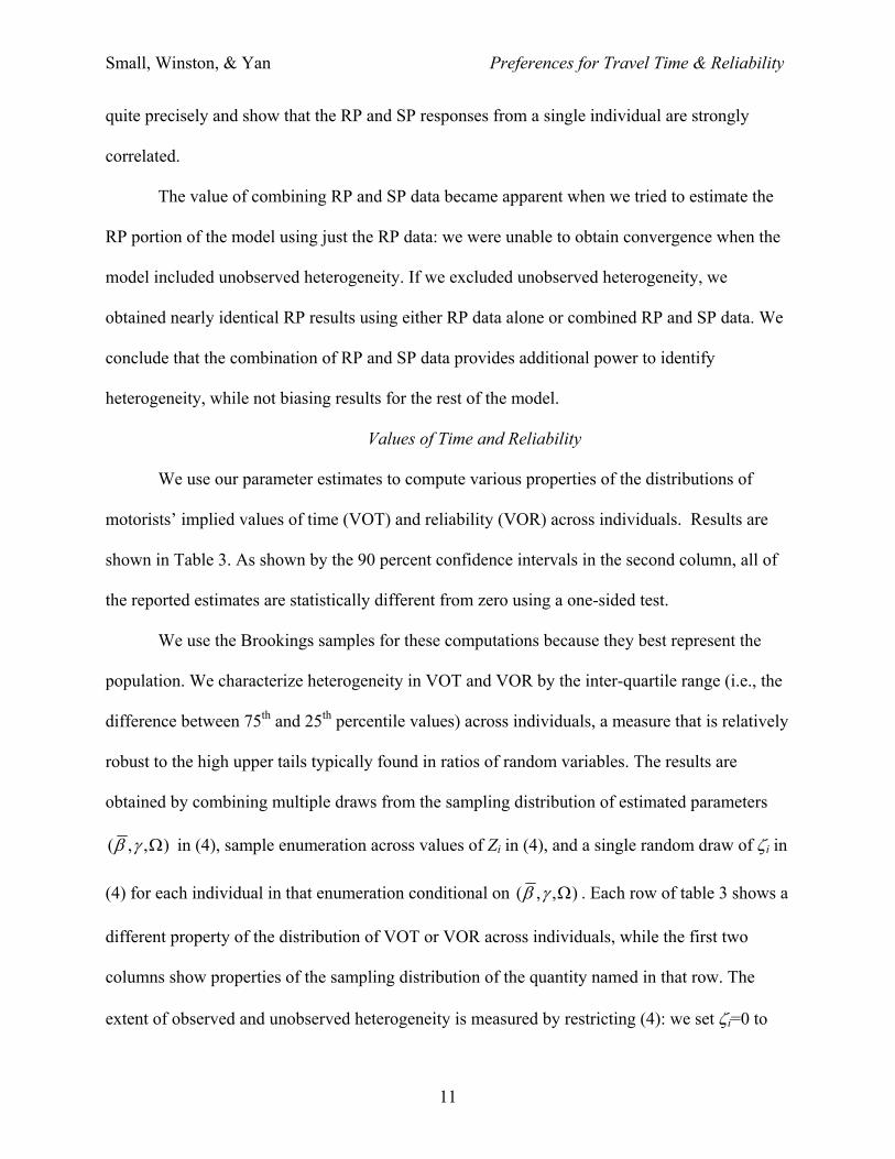
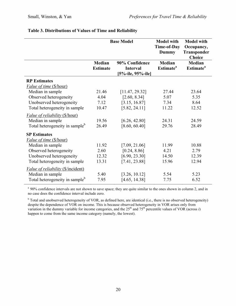
Values of Time and Reliability

We use our parameter estimates to compute various properties of the distributions of

motorists’ implied values of time (VOT) and reliability (VOR) across individuals. Results are

shown in Table 3. As shown by the 90 percent confidence intervals in the second column, all of

the reported estimates are statistically different from zero using a one-sided test.

We use the Brookings samples for these computations because they best represent the

population. We characterize heterogeneity in VOT and VOR by the inter-quartile range (i.e., the

difference between 75th and 25th percentile values) across individuals, a measure that is relatively

robust to the high upper tails typically found in ratios of random variables. The results are

obtained by combining multiple draws from the sampling distribution of estimated parameters

),,( Ωγβ in (4), sample enumeration across values of Zi in (4), and a single random draw of ζi in

(4) for each individual in that enumeration conditional on ),,( Ωγβ . Each row of table 3 shows a

different property of the distribution of VOT or VOR across individuals, while the first two

columns show properties of the sampling distribution of the quantity named in that row. The

extent of observed and unobserved heterogeneity is measured by restricting (4): we set ζi=0 to


12

account for only observed heterogeneity, and we replace Zi by its sample mean to account for

only unobserved heterogeneity.

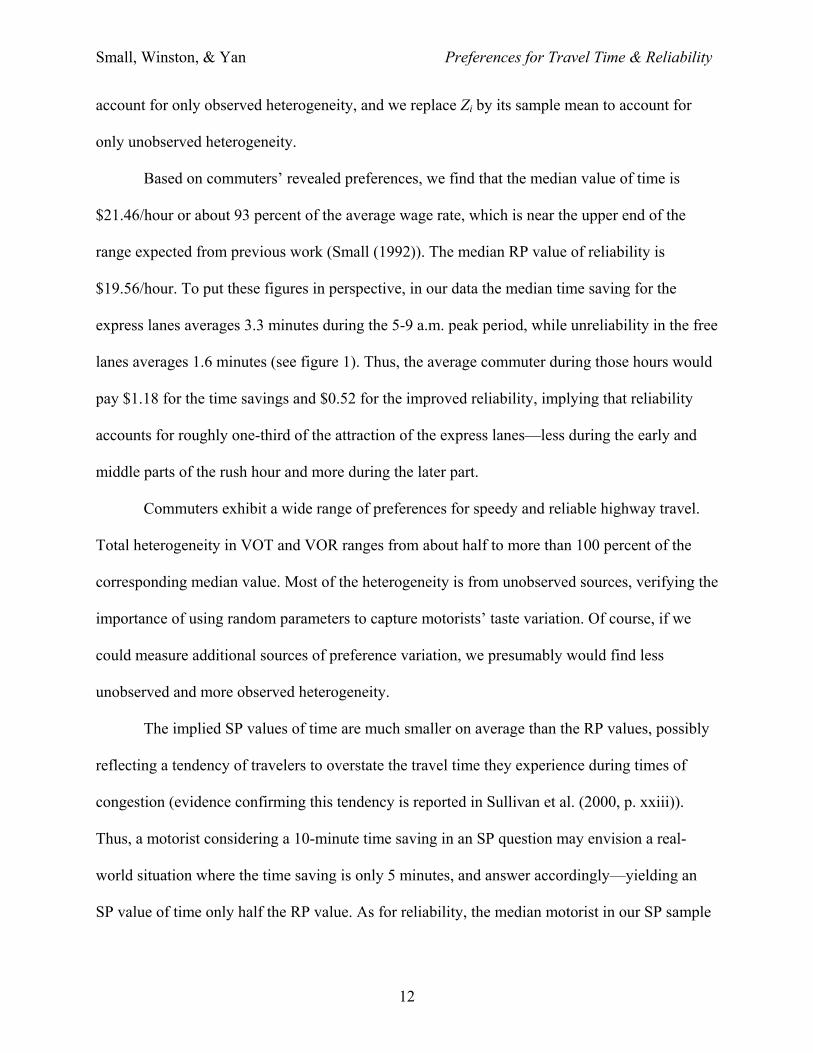
Based on commuters’ revealed preferences, we find that the median value of time is

$21.46/hour or about 93 percent of the average wage rate, which is near the upper end of the

range expected from previous work (Small (1992)). The median RP value of reliability is

$19.56/hour. To put these figures in perspective, in our data the median time saving for the

express lanes averages 3.3 minutes during the 5-9 a.m. peak period, while unreliability in the free

lanes averages 1.6 minutes (see figure 1). Thus, the average commuter during those hours would

pay $1.18 for the time savings and $0.52 for the improved reliability, implying that reliability

accounts for roughly one-third of the attraction of the express lanes—less during the early and

middle parts of the rush hour and more during the later part.

Commuters exhibit a wide range of preferences for speedy and reliable highway travel.

Total heterogeneity in VOT and VOR ranges from about half to more than 100 percent of the

corresponding median value. Most of the heterogeneity is from unobserved sources, verifying the

importance of using random parameters to capture motorists’ taste variation. Of course, if we

could measure additional sources of preference variation, we presumably would find less

unobserved and more observed heterogeneity.

The implied SP values of time are much smaller on average than the RP values, possibly

reflecting a tendency of travelers to overstate the travel time they experience during times of

congestion (evidence confirming this tendency is reported in Sullivan et al. (2000, p. xxiii)).

Thus, a motorist considering a 10-minute time saving in an SP question may envision a real-

world situation where the time saving is only 5 minutes, and answer accordingly—yielding an

SP value of time only half the RP value. As for reliability, the median motorist in our SP sample


13

exhibits a willingness to pay of $0.54 per trip to reduce the frequency of 10-minute delays from

0.2 to 0.1.

Sensitivity to Identifying Assumption and Alternative Specifications

We have implicitly assumed that any unobserved influences on lane choice do not vary

systematically by time of day; if they did, they would be correlated with cost, time, and

reliability and therefore bias those coefficients. The validity of this assumption depends partly on

how well our observed variables capture taste variation across times of day. Fortunately, we have

many variables that play this role including income, trip distance, trip purpose, flexibility of

arrival time, sex, age, household size, occupation, marital status, and education. For example, a

motorist’s sex is likely to be an important source of taste variation; we know it is correlated with

time of day because females constitute only 15% of those commuters traveling during the

interval 4-5 a.m., but 39% of the 7-8 a.m. group. Similarly with trip purpose: the proportion of

respondents whose trips are work trips varies from 100% at the earliest time to 58% at the latest

time.

A more formal test takes advantage of the fact that 55 members of the SP sample,

providing 433 observations, told us the time of day at which their actual trip normally took place.

In the SP sample, travel time and reliability are uncorrelated with the time of day as part of the

survey design, so we can include time-of-day dummies in an SP-only model restricted to these

observations while still measuring other parameters with precision. We can then compare the

results with and without these dummies to see whether VOT and VOR are affected. We used five

time-of-day dummies, one for each hour of the morning period other than a base hour defined as

7-8 a.m. Their estimated coefficients were not jointly significantly different from zero.

Moreover, including the dummies decreased the median SP values of time and reliability less


14

than 10 percent and increased the amount of unobserved heterogeneity (as measured by the inter-

quartile range) less than 8 percent. Hence, based on the SP data our results are robust to omitted

time-of-day-related influences.

We performed a further check by re-estimating the joint RP/SP model, using all the data

and including a dummy variable for travel at 7-8 a.m., the one period that appeared different

from all the others in the SP-only experiment just described. (We set this dummy variable to zero

for those 26 people not answering the time-of-day question and treated them like a separate

sample, with their own alternative-specific constant and error variance.) The estimated

coefficient for the time-of-day dummy is –1.64 with standard error 1.29. The third column of

table 3 shows the resulting VOT and VOR estimates; the 90 percent confidence intervals, not

shown, still exclude zero in all cases. Including the time-of-day dummy increases modestly the

estimated median RP values of time and reliability, and also increases slightly the amount of

unobserved heterogeneity in those values. Therefore, our main conclusions—that values of time

and reliability are high and contain considerable unobserved heterogeneity—are if anything

strengthened. We do lose precision by incorporating the time dummy, so we offer the base model

as containing our best estimates.

It is also possible that the demand elasticity for the toll road varies by time of day, in a way

that is not captured by our observables. Thus, if the toll-lane operator systematically sets prices

higher than they otherwise would be whenever the elasticity is small in magnitude, and if

unobservable factors are correlated with both the level and the elasticity of demand, then price

would not be exogenous and its coefficient would be over- or underestimated depending on the

signs of the correlations. Any resulting bias to the estimated VOT and VOR would be smaller,

because the time savings and unreliability variables are causally related to price through congestion


15

in the regular lanes, so their coefficients would be biased in the same direction as that of price.

We examined the robustness to assumed cross-equation constraints by estimating models

both with fewer and with more constraints relating the RP and SP coefficients. We computed the

resulting distributions of the values of time and reliability, obtaining results virtually

indistinguishable from those of the base model. Furthermore, we found using likelihood-ratio

tests that we could not reject our preferred specification against less constrained models. Indeed,

we found that we could have imposed an additional constraint equating the cost coefficients, but

we preferred not to do so because this coefficient is critical to our VOT and VOR calculations.

Finally, we explored potential simultaneity bias by estimating a model explaining the

simultaneous choice of vehicle occupancy, transponder acquisition, and lane by RP respondents,

as well as lane only by SP respondents. We created nine alternatives from the permitted

combinations of these choices. Conditional on the random coefficients, including a random

constant for the transponder, choice among the nine alternatives is multinomial logit; but this is

less restrictive than it appears because our error structure mimics a nested logit, as described by

Brownstone and Train (1999). The resulting VOT and VOR distributions, summarized in the last

column of Table 3, are similar to those from the base model and support our earlier arguments

that other choices would have little impact on our findings. It is useful to note that the joint RP

model can be expressed as a selection model in which transponder choice determines whether

lane choice is observed. The random constant for transponder choice then allows the correlation

between the selection equation and the lane-choice equation to be estimated, rather than being

imposed by the logit functional form. (As it happens, we could not reject the hypothesis that the

random constant has zero variance.) But the selection model contains exclusion restrictions

based solely on statistical insignificance, so we are assuming that it is identified by the mixed-


16

logit functional form with the random constant.

6. Conclusion

By combining the power of RP and SP data, using a random-parameters model, and

constructing improved measures of reliability, we are able to measure properties of travel

preferences that have eluded other studies. We find that travel time and its predictability are

highly valued by motorists and that there is significant heterogeneity in these values.

Motorists’ varying preferences for travel time and reliability have important implications

for road pricing policy. As noted earlier, theoretical studies find that substantial heterogeneity is

necessary for value pricing as currently practiced to create significant benefits. The amount of

heterogeneity found here is likely to generate such benefits. For example, in Small and Yan

(2001), an inter-quartile difference of half the median value of time (roughly what we find in

revealed behavior) approximately quadruples the maximum benefit attainable from second-best

pricing when there is no heterogeneity.

Accounting for preference variation could also enhance the political viability of pricing.

We show in a companion paper (Small, Winston, and Yan (2005)) that differentiated road prices

can be designed, based on the distributions of values of time and reliability obtained here, to

produce greater efficiency gains than current experiments while retaining or even increasing their

distributional advantages over comprehensive road pricing. Thus there may be a politically

feasible compromise between value pricing as now practiced, which is not very efficient, and first-

best congestion pricing, which introduces severe disparities in direct welfare impact.

In a nutshell, our confirmation of significant preference heterogeneity among travelers

offers policymakers a long-awaited opportunity to address the stalemates that impede

transportation policy in congested cities.


17

Figure 1. Time Savings from Express Lanes

4 5 6 7 8 9 100

1.2

2.4

3.6

4.8

6

7.2

8.4

9.6

10.8

12

Time of Day Passing Toll Sign (a.m.)

Tim

e S

avin

g (m

in.)

Data Points (left axis)

4 5 6 7 8 9 10

0

1.2

2.4

3.6

4.8

6

Dis

pers

ion

of T

ime

Sav

ing

(80%

−ile

− M

edia

n)

Dispersion (right axis)

Median (left axis)

Note: The dashed lines are 90 percent confidence intervals. Dispersion is difference between the 80th and 50th percentiles.

Table 1. Descriptive Statistics Value or Fraction of Sample Cal Poly-RP Brookings-RP Brookings-SP Choose 91X (RP dependent variable) 0.26 0.25 Time Period of Trip (RP): 4:00am-7:00am 0.56 0.54 7:00am-8:00am 0.20 0.21 8:00am-10:00am 0.24 0.25 Age (years): <30 0.11 0.12 0.10 30-50 0.62 0.62 0.64 Household Income ($/year): <60,000 0.38 0.83 0.83 >100,000 0.22 0.02 0.04 Female Dummy 0.32 0.37 0.37 Mean Actual Trip Distance (Miles) 34.2 44.8 42.6 Number of Respondents 438 84 81 Number of Observations 438 377 633


18

Table 2. Parameter Estimates of Lane Choice Model

Dependent Variable: 1 if chose toll lanes, 0 otherwise Independent Variable:

Coefficient

(standard error)a RP Variables

Constant: Brookings sub-sample (BR

θ ) 0.1489 (0.8931)

Constant: Cal Poly sub-sample (C

θ ) -1.6349 (1.1040)

Cost ($) -1.8705 (0.5812)

Cost x dummy for medium household inc. ($60-100K) 0.5438 (0.2549)

Cost x dummy for high household income (>$100,000) 1.1992 (0.3849)

Median travel time (min.) x trip distance (units: 10 mi.) -0.4088 (0.1536)

Median travel time x (trip distance squared) 0.0695 (0.0276)

Median travel time x (trip distance cubed) -0.0029 (0.0012)

Unreliability of travel time (minutes) -0.5778 (0.2435)

SP Variables

Constant (BS

θ ) -1.6107 (0.8943)

Standard deviation of constant ( ξσ ) 0.4800 (0.6305)

Cost -1.0008 (0.2849)

Cost x dummy for medium household inc. ($60-100K) -0.2317 (0.5407)

Cost x dummy for high household income (>$100,000) 0.2842 (0.9714)

Travel time (min.) × long-commute dummy (>45 min.) -0.1965 (0.0522)

Travel time × (1 − long-commute dummy) -0.2146 (0.0618)

Unreliability of travel time (probability of late arrival) -5.6292 (2.3819)

Pooled Variables

Female dummy 1.3267 (0.6292)

Age 30-50 dummy 1.2362 (0.5121)

Flexible arrival-time dummy 0.5903 (0.6994)

Household size (number of people) -0.5497 (0.2248)

Standard dev. of coeff’s of travel time (in Ω) 0.1658 (0.0457)

Ratio of std. dev. to mean for coeff’s of unreliability (in Ω) 1.0560 (0.2754)


19

Other Parameters Scale parameter: Cal Poly sample ( Cµ ) 0.4118 (0.1688)

Scale parameter: SP sample ( BSµ ) 1.3368 (0.3741)

Correlation parameter, Brookings RP and SP ( )ρ 3.2882 (0.8320)

Summary Statistics Number of observations 1155 Number of persons 548 Number of replications (R) 4,500 Log-likelihood -501.57 Pseudo R2 0.3704

Implied Elasticities of Demand for Express Laneb Toll in express lanes -1.588 (0.504) Median travel time in free lanes 0.727 (0.331) Unreliability in free lanes 0.374 (0.166)

a Standard errors are the “sandwich” estimates of Lee (1995), obtained from ( ) ( ) 11ˆ −− −−= HPHV , where H is the Hessian of the simulated log-likelihood function and P is the outer product of its gradient vector (both calculated numerically). This estimate accounts for simulation error in the likelihood. b Express lane usage is computed by aggregating individual choice probabilities over the Brookings RP sample. Each probability is calculated by simulated integration over the distributions defined by (4), conditional on all estimated parameters of the model; the calculation is then repeated after a 10% increase in the toll, median travel-time saving, or unreliability facing each individual, and an elasticity calculated. This process is repeated for each of 1,000 random draws of the estimated parameters from their sampling distribution. The numbers reported are the empirical mean and standard deviation across the 1,000 resulting elasticities.


20

Table 3. Distributions of Values of Time and Reliability

Base Model Model with Time-of-Day

Dummy

Model with Occupancy,

Transponder Choice

Median Estimate

90% Confidence Interval

[5%-ile, 95%-ile]

Median Estimatea

Median Estimatea

RP Estimates Value of time ($/hour) Median in sample 21.46 [11.47, 29.32] 27.44 23.64 Observed heterogeneity 4.04 [2.60, 8.34] 5.07 5.35 Unobserved heterogeneity 7.12 [3.15, 16.87] 7.34 8.64 Total heterogeneity in sample 10.47 [5.82, 24.11] 11.22 12.52 Value of reliability ($/hour) Median in sample

19.56

[6.26, 42.80]

24.31

24.59

Total heterogeneity in sampleb 26.49 [8.60, 60.40] 29.76 28.49

SP Estimates Value of time ($/hour) Median in sample 11.92 [7.09, 21.06] 11.99 10.88 Observed heterogeneity 2.60 [0.24, 8.86] 4.21 2.79 Unobserved heterogeneity 12.32 [6.90, 23.30] 14.50 12.39 Total heterogeneity in sample 13.31 [7.41, 23.88] 15.96 12.94 Value of reliability ($/incident) Median in sample 5.40 [3.26, 10.12] 5.54 5.23 Total heterogeneity in sampleb 7.95 [4.65, 14.38] 7.75 6.52

a 90% confidence intervals are not shown to save space; they are quite similar to the ones shown in column 2, and in no case does the confidence interval include zero.

b Total and unobserved heterogeneity of VOR, as defined here, are identical (i.e., there is no observed heterogeneity) despite the dependence of VOR on income. This is because observed heterogeneity in VOR arises only from variation in the dummy variable for income categories, and the 25th and 75th percentile values of VOR (across i) happen to come from the same income category (namely, the lowest).


21

References Ben-Akiva, M., and T. Morikawa (1990), “Estimation of Travel Demand Models from Multiple Data Sources,” in Koshi, M., ed., Transportation and Traffic Theory. New York: Elsevier, pp. 461-478. Brownstone, D., and K. Train (1999), “Forecasting New Product Penetration with Flexible Substitution Patterns,” Journal of Econometrics, 89, pp. 109-129. Calfee, J., and C. Winston (1998), “The Value of Automobile Travel Time: Implications for Congestion Policy,” Journal of Public Economics, 69, pp. 83-102. Calfee, J., C.Winston, and R. Stempski (2001), “Econometric Issues in Estimating Consumer Preferences from Stated Preference Data: A Case Study of the Value of Automobile Travel Time,” Review of Economics and Statistics, 83, pp. 699-707. Hensher, D. A. (2001), “The Valuation of Commuter Travel Time Savings for Car Drivers: Evaluating Alternative Model Specifications,” Transportation, 28, pp. 101-118. Koenker, R., and G. S. Basset (1978), “Regression Quantiles,” Econometrica, 46, pp. 33-50. Lee, L. (1995), “Asymptotic Bias in Simulated Maximum Likelihood Estimation of Discrete Choice Models,” Econometric Theory, 11, pp. 437-483. McFadden, D., and K. Train (2000), “Mixed MNL Models for Discrete Response,” Journal of Applied Econometrics, 15, pp. 447-470. Noland, R. B., and K. A. Small (1995), "Travel-Time Uncertainty, Departure Time Choice, and the Cost of Morning Commutes," Transportation Research Record, 1493, pp. 150-158. Parkany, E. A. (1999), Traveler Responses to New Choices: Toll vs. Free Alternatives in a Congested Corridor, Ph.D. Dissertation, University of California at Irvine. Small, K. A. (1992), Urban Transportation Economics, Vol. 51 of Fundamentals of Pure and Applied Economics Series, Harwood Academic Publishers. Small. K. A. and C. Winston (1999), “The Demand for Transportation: Models and Applications,” in J. Gomez-Ibanez, W. Tye, and C. Winston, editors, Essays in Transportation Economics and Policy: A Handbook in Honor of John R. Meyer, Washington, DC: Brookings Institution Press. Small, K. A., C. Winston, and J. Yan (2005): “Differentiated Pricing, Express Lanes, and Carpools: Exploiting Heterogeneous Preferences in Policy Design,” Working Paper, Dept. of Economics, University of California at Irvine.


22

Small, K. A. and J. Yan (2001), “The Value of “Value Pricing” of Roads: Second-Best Pricing and Product Differentiation,” Journal of Urban Economics, 49, pp. 310-336. Sullivan, E., with K. Blakely, J. Daly, J. Gilpin, K. Mastako, K.A. Small, and J. Yan (2000), Continuation Study to Evaluate the Impacts of the SR 91 Value-Priced Express Lanes: Final Report. Dept. of Civil and Environmental Engineering, California Polytechnic State Univ. at San Luis Obispo, Dec. (http://ceenve.ceng.calpoly.edu/sullivan/SR91/, accessed Feb. 14, 2004). Train, K. (2001), “A Comparison of Hierarchical Bayes and Maximum Simulated Likelihood for Mixed Logit,” working paper, Dept. of Economics, Univ. of California at Berkeley, May (http://elsa.berkeley.edu/~train/papers.html, accessed Feb. 14, 2004). Train, K. (2003), Discrete Choice Methods with Simulation, Cambridge, UK: Cambridge University Press. Verhoef, E.T. and K.A. Small (2004), "Product Differentiation on Roads: Constrained Congestion Pricing with Heterogeneous Users," Journal of Transport Economics and Policy 38, pp. 127-156. Wardman, M. (2001), “A Review of British Evidence of Time and Service Quality Valuations,” Transportation Research E: Logistics and Transportation Review, 37, pp. 107-128.

uncovering the distribution of motoristsâ€™ preferences for travel

Documents