unclassified std/doc(2016)3 - oecd
TRANSCRIPT

Unclassified STD/DOC(2016)3 Organisation de Coopération et de Développement Économiques Organisation for Economic Co-operation and Development 10-May-2016
___________________________________________________________________________________________
_____________ English - Or. English STATISTICS DIRECTORATE
BIG DATA MEASURES OF WELL-BEING: EVIDENCE FROM A GOOGLE WELL-BEING INDEX
IN THE UNITED STATES
WORKING PAPER No.69
Contact: Fabrice Murtin, Statistics Directorate, +33 (0)1 45 24 76 08; [email protected]
JT03395559
Complete document available on OLIS in its original format
This document and any map included herein are without prejudice to the status of or sovereignty over any territory, to the delimitation of
international frontiers and boundaries and to the name of any territory, city or area.
ST
D/D
OC
(2016)3
Un
classified
En
glish
- Or. E
ng
lish
Cancels & replaces the same document of 29 April 2016

STD/DOC(2016)3
2
BIG DATA MEASURES OF WELL-BEING:
EVIDENCE FROM A GOOGLE WELL-BEING INDEX IN THE UNITED STATES
Yann Algan, Elizabeth Beasley, Florian Guyot, Kazuhito Higa, Fabrice Murtin and Claudia Senik1
1 Yann Algan, Sciences-Po: [email protected]; Elizabeth Beasley, CEPREMAP:
[email protected]; Florian Guyot, Sciences Po; Kazuhito Higa, Kyushu University,
formerly an intern at the OECD: [email protected]; Fabrice Murtin, Economist at the OECD
and Sciences-Po (Corresponding author): [email protected]; Claudia Senik, Université Paris-
Sorbonne and Paris School of Economics: [email protected]. Algan, Beasley and Senik are grateful to
CEPREMAP for financial support. Yann Algan has received the financial support of the ERC Advanced
Grant. This paper has received the technical support from the Medialab at Sciences Po and the authors are
especially grateful to Paul Girard, Guillaume Plique and Mathieu Jacomy. We also thank Melissa Leroux
for excellent research assistance. This document expresses the views of the authors and does not
necessarily reflect the official views of the OECD.

STD/DOC(2016)3
3
OECD STATISTICS WORKING PAPER SERIES
The OECD Statistics Working Paper Series - managed by the OECD Statistics Directorate - is
designed to make available in a timely fashion and to a wider readership selected studies prepared by
OECD staff or by outside consultants working on OECD projects. The papers included are of a technical,
methodological or statistical policy nature and relate to statistical work relevant to the Organisation. The
Working Papers are generally available only in their original language - English or French - with a
summary in the other.
OECD Working Papers should not be reported as representing the official views of the OECD or of its
member countries. The opinions expressed and arguments employed are those of the author
Working Papers describe preliminary results or research in progress by the author and are published to
stimulate discussion on a broad range of issues on which the OECD works. Comments on Working Papers
are welcomed, and may be sent to the Statistics Directorate, OECD, 2 rue André-Pascal, 75775 Paris
Cedex 16, France.
The release of this working paper has been authorised by Martine Durand, OECD Chief Statistician
and Director of the OECD Statistics Directorate.
www.oecd.org/std/publicationsdocuments/workingpapers/

STD/DOC(2016)3
4
ABSTRACT
We build an indicator of individual subjective well-being in the United States based on Google
Trends. The indicator is a combination of keyword groups that are endogenously identified to fit with the
weekly time-series of subjective well-being measures disseminated by Gallup Analytics. We find that
keywords associated with job search, financial security, family life and leisure are the strongest predictors
of the variations in subjective well-being. The model successfully predicts the out-of-sample evolution of
most subjective well-being measures at a one-year horizon.
RÉSUMÉ
Un indicateur de bien-être subjectif est construit pour les États-Unis sur la base des données de
Google Trends. L’indicateur est une combinaison de mots-clés qui sont identifiés pour reproduire les séries
hebdomadaires de bien-être subjectif de Gallup Analytics. Nous trouvons que les mots-clés associés à la
recherche d’emploi, à la sécurité financière, à la vie de famille et aux loisirs sont les plus forts prédicteurs
des variations du bien-être subjectif. Le modèle prévoit l’évolution hors échantillon de la plupart des
mesures de bien-être à l’horizon d’un an.

STD/DOC(2016)3
5
TABLE OF CONTENTS
BIG DATA MEASURES OF WELL-BEING: EVIDENCE FROM A GOOGLE WELL-BEING INDEX
IN THE UNITED STATES ............................................................................................................................. 2 ABSTRACT .................................................................................................................................................... 4 RÉSUMÉ ......................................................................................................................................................... 4
1. Introduction .......................................................................................................................................... 6 2. The Data ............................................................................................................................................... 7
2.1. Gallup Data .................................................................................................................................. 7 2.2. Google Trends Data ..................................................................................................................... 9
3. Empirical Framework ......................................................................................................................... 10 3.1. Big Data, Noisy Data and High Dimensionality ....................................................................... 10 3.2. Category Construction ............................................................................................................... 11 3.3. Bayesian Model Averaging ....................................................................................................... 17 3.4. Model Selection and Out-of-Sample Testing ............................................................................ 18
4. How to Google Subjective Well-Being in the United States? ............................................................ 19 4.1. A Model of SWB in the United States....................................................................................... 19 4.2. Variance Decomposition ........................................................................................................... 21 4.3. Predicting SWB in the United States and Reliability of the Model ........................................... 22
5. Conclusion .......................................................................................................................................... 25 REFERENCES .............................................................................................................................................. 26 APPENDIX A. BIG DATA ISSUES ............................................................................................................ 29 APPENDIX B. EXPLORATORY FACTOR ANALYSIS ........................................................................... 32 APPENDIX C. BAYESIAN AVERAGING MODEL RESULTS ............................................................... 36
Tables
Table 1. Category Components ........................................................................................................... 13 Table 2. Regression of Categories on Subjective Well-Being Data .................................................... 20 Table 3. Decomposition of the Explained Variance of SWB variables ............................................... 22 Table 4. Correlation Between Predicted and Observed SWB values (Smoothed) .............................. 23 Table B1. Factor Loading for Material Conditions Variables ................................................................ 32 Table B2. Factor Loading for Social Variables ...................................................................................... 33 Table B3. Factor Loading for Health and Wellness Variables ............................................................... 34
Figures
Figure 1. Subjective Well Being Variables over time............................................................................. 8 Figure 2. Category Variables over time ................................................................................................ 15 Figure 3. Comparison of selected category composites to administrative data series .......................... 17 Figure 4. Predictions and Observed SWB (Training Data inside the red lines, Test Data outside) ...... 24 Figure A1. “Spikes” and the Divorce of Kim Kardashian ....................................................................... 29 Figure A2. “Cliffs” and Mace Spray ........................................................................................................ 30 Figure A3. Adjustment for the January 2011 Discontinuity .................................................................... 31 Figure A4. Time trends in “Teeth hurt” ................................................................................................... 31

STD/DOC(2016)3
6
1. Introduction
1. There is a growing interest in social sciences in going beyond the income-based approach of
human development by using new measures of wellbeing (Stiglitz et al., 2009). In particular, GDP does not
measure non-market social interactions such as friendship, family happiness, moral values or the sense of
purpose in life. This motivates the recourse to subjective self-reported measures of well-being, such as Life
Satisfaction (i.e. answers to the question: “All things considered, how satisfied are you with your life as a
whole those days?”), which economists increasingly use as a direct measure of utility.2 Political leaders
have embraced this move by calling for representative surveys of well-being to guide their policy, as
illustrated by the Cameron’s commission of well-being in UK. In spite of these achievements, subjective
well-being measures still raise a number of challenges and concerns among economists. First, they are not
based on revealed behavior and choices, and are affected by the limits inherent to all self-reports (Deaton,
2013). Subjective well-being is also multidimensional (Kahneman and Deaton, 2010; Steptoe et al. 2014)
and some aspects, especially pain or chronic disability are difficult to capture. Second, survey questions on
subjective well-being are limited in coverage, time and space, which most of the time eliminates the
possibility of measuring it with the appropriate business-cycle frequency and local level for policy
decisions. Third, questions are sensitive to wording and ordering effects if the survey is changed (Deaton,
2013).
2. This paper contributes to this new research agenda by showing how Big Data can improve our
understanding of the foundations of well-being. A major consequence of the accelerated digitization of
social life is the traceability of social relations, embedded in large datascapes, such as Google, Facebook,
Twitters or the Blogosphere. The quantification of those social traces is of considerable interest for social
scientists. However, as stated by Lazer et al. (1999), while the capacity to collect and analyze massive
amount of data has transformed the fields of physics and biology, such attempts have been much slower in
social sciences. This paper illustrates the potential use of Big Data for both the measurement and the
analysis of subjective well-being.
3. The first advantage of these data is that they offer social scientists the possibility to observe
people’s behavior, such as Google queries, and not just opinions. Second, rather than relying on the
answers to pre-defined questions, social scientists can listen to what people say. This approach of revealed
preferences unveils a reflexive picture of society because it allows the main concerns of citizens (and the
priority ranking of those concerns) to emerge spontaneously, and it complements as such the information
captured by GDP. In a nutshell, these data are based on the actual behavior of people when they search for
information and they endogenously elicit the relative importance of people’s concerns.
4. The second advantage of these data is their timeliness as they offer an immediate source of
information for policy-makers, who are often confronted with short-term horizons and data scarcity in the
midst of the decision-making process. Moreover, they are available at a local level - as long as internet
penetration and use is sufficient to obtain statistical representativeness. Finally, Big Data are often made
available for free.
2 Subjective well-being measures have been used to test a variety of potential determinants of wellbeing such
as income, unemployment, inflation, health status, income inequality and income comparisons (see, for
example, Helliwell et al. 2015).
STD/DOC(2016)3
7
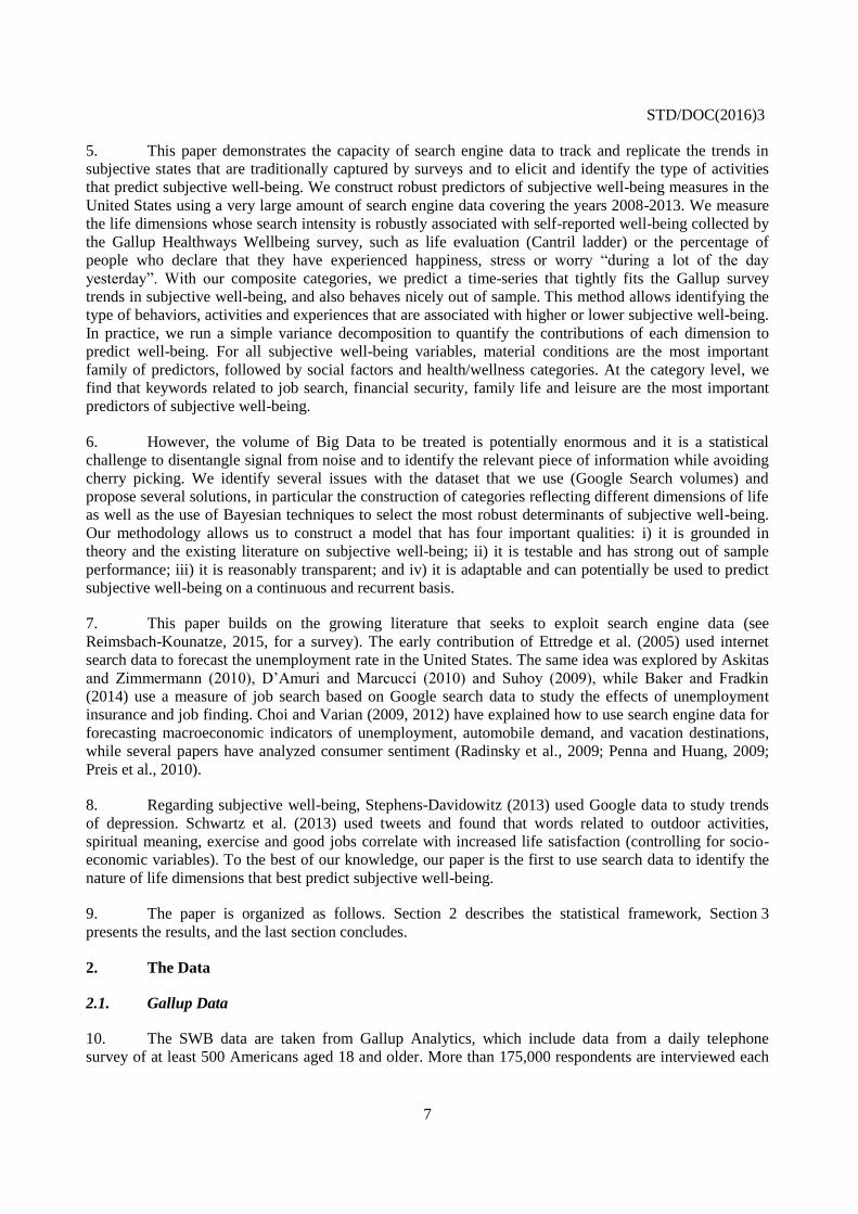
5. This paper demonstrates the capacity of search engine data to track and replicate the trends in
subjective states that are traditionally captured by surveys and to elicit and identify the type of activities
that predict subjective well-being. We construct robust predictors of subjective well-being measures in the
United States using a very large amount of search engine data covering the years 2008-2013. We measure
the life dimensions whose search intensity is robustly associated with self-reported well-being collected by
the Gallup Healthways Wellbeing survey, such as life evaluation (Cantril ladder) or the percentage of
people who declare that they have experienced happiness, stress or worry “during a lot of the day
yesterday”. With our composite categories, we predict a time-series that tightly fits the Gallup survey
trends in subjective well-being, and also behaves nicely out of sample. This method allows identifying the
type of behaviors, activities and experiences that are associated with higher or lower subjective well-being.
In practice, we run a simple variance decomposition to quantify the contributions of each dimension to
predict well-being. For all subjective well-being variables, material conditions are the most important
family of predictors, followed by social factors and health/wellness categories. At the category level, we
find that keywords related to job search, financial security, family life and leisure are the most important
predictors of subjective well-being.
6. However, the volume of Big Data to be treated is potentially enormous and it is a statistical
challenge to disentangle signal from noise and to identify the relevant piece of information while avoiding
cherry picking. We identify several issues with the dataset that we use (Google Search volumes) and
propose several solutions, in particular the construction of categories reflecting different dimensions of life
as well as the use of Bayesian techniques to select the most robust determinants of subjective well-being.
Our methodology allows us to construct a model that has four important qualities: i) it is grounded in
theory and the existing literature on subjective well-being; ii) it is testable and has strong out of sample
performance; iii) it is reasonably transparent; and iv) it is adaptable and can potentially be used to predict
subjective well-being on a continuous and recurrent basis.
7. This paper builds on the growing literature that seeks to exploit search engine data (see
Reimsbach-Kounatze, 2015, for a survey). The early contribution of Ettredge et al. (2005) used internet
search data to forecast the unemployment rate in the United States. The same idea was explored by Askitas
and Zimmermann (2010), D’Amuri and Marcucci (2010) and Suhoy (2009), while Baker and Fradkin
(2014) use a measure of job search based on Google search data to study the effects of unemployment
insurance and job finding. Choi and Varian (2009, 2012) have explained how to use search engine data for
forecasting macroeconomic indicators of unemployment, automobile demand, and vacation destinations,
while several papers have analyzed consumer sentiment (Radinsky et al., 2009; Penna and Huang, 2009;
Preis et al., 2010).
8. Regarding subjective well-being, Stephens-Davidowitz (2013) used Google data to study trends
of depression. Schwartz et al. (2013) used tweets and found that words related to outdoor activities,
spiritual meaning, exercise and good jobs correlate with increased life satisfaction (controlling for socio-
economic variables). To the best of our knowledge, our paper is the first to use search data to identify the
nature of life dimensions that best predict subjective well-being.
9. The paper is organized as follows. Section 2 describes the statistical framework, Section 3
presents the results, and the last section concludes.
2. The Data
2.1. Gallup Data
10. The SWB data are taken from Gallup Analytics, which include data from a daily telephone
survey of at least 500 Americans aged 18 and older. More than 175,000 respondents are interviewed each

STD/DOC(2016)3
8
year, and over 2 million interviews have been conducted to date since the start of the survey in 2008. The
survey includes 6 measures of self-reported positive emotions (happiness, learning, life evaluations today
and in 5 years, laugh, being respected) as well as 4 measures of negative emotions (anger, sadness, stress,
worry). The time span covers 300 weeks from January 6, 2008 to January 4, 2014.
Figure 1. Subjective Well Being Variables over time
6.6
6.7
6.8
6.9
77.1
life
_ev
al_
01jan2008 01jan2010 01jan2012 01jan2014time
Life Evaluation
7.4
7.5
7.6
7.7
7.8
7.9
life
_ev
al_5yr_
01jan2008 01jan2010 01jan2012 01jan2014time
Life Evaluation in 5 years
84
86
88
90
hap
pin
ess_
01jan2008 01jan2010 01jan2012 01jan2014time
Happiness
78
80
82
84
86
laugh_
01jan2008 01jan2010 01jan2012 01jan2014time
Laugh
50
55
60
65
70
lear
n_
01jan2008 01jan2010 01jan2012 01jan2014time
Learn
89
90
91
92
93
94
resp
ect_
01jan2008 01jan2010 01jan2012 01jan2014time
Respect
11
12
13
14
15
16
anger
_
01jan2008 01jan2010 01jan2012 01jan2014time
Anger
30
35
40
45
stre
ss_
01jan2008 01jan2010 01jan2012 01jan2014time
Stress

STD/DOC(2016)3
9
11. Figure 1 depicts these ten indicators over the period. The consequences of the Great Recession
are visible on most SWB indices: life evaluation today and in 5 years, happiness and laugh dropped
significantly in 2008-2009, while the percentages of people experiencing worry, anger, stress and sadness
increased at the same time. A second observation concerns the cyclicality of these variables, which all
display large seasonal swings.
2.2. Google Trends Data
12. Our ‘Big Data’ here consist of the search frequency of keywords on Google, which are available
from Google Trends. The initial list of keywords is selected as follows. We extract two long lists of
keywords potentially linked to SWB outcomes. The first one comes from the OECD Better Life Index
Online Database, which records answers from data users to the question “What does a Better Life mean to
you?” The second one is based on the American Time Use Survey, which records the daily activities
undertaken by US citizens as well as the positive or negative emotions that are associated with these
episodes. This selection method allows us to avoid cherry picking a limited set of search queries on
Google. On the other hand, survey-based keywords may be disconnected from the day-to-day life of
Americans if they do not include their usual internet queries or do not reflect their practical living
conditions. As a consequence, we have added a set of keywords that were likely to be relevant to different
life experiences related to subjective well-being: this ranges from job concerns (e.g. the website ‘getajob’),
poverty (‘coupons’) or family stress (‘women shelter’). In total, the initial database contains 845 keywords,
split into 144 for the BLI, 95 for the US time-use data and 606 from our own judgment.
13. The search volumes obtained from Google Trends pose several challenges for estimation.3 First,
there may be sharp spikes in the popularity of a word. While some of these spikes are surely related to the
degree to which the concept represented by this word is important in people’s lives, others are less directly
related. The example of the spike in “divorce” searches induced by Kim Kardashian’s precipitous divorce
from Kris Humphries in October 2010 is shown in Appendix A. This is a concern for estimation as it
3 The Google Trends data on search volume is not the raw search volume; rather it is the proportion of total
searches over a given period that included that keyword, normalized so that the highest volume over the
period is equal to 100. This has several consequences: first, the value of the series obtained directly from
Google Trends is difficult to interpret, as it depends not only on the volume of searches for a given word
but also on the volume of other searches. Second, the value of the series on any given day cannot be
compared between terms, since they are normalized to the maximum value by term. To deal with this issue,
we normalize all search volumes so that they have a mean of zero and a standard deviation of one, since we
are interested in how volume changes within a given term (rather than which terms have the highest search
volumes overall).
26
28
30
32
34
36
worr
y_
01jan2008 01jan2010 01jan2012 01jan2014time
Worry
16
18
20
22
sadnes
s_
01jan2008 01jan2010 01jan2012 01jan2014time
Sadness

STD/DOC(2016)3
10
creates a risk of over-fitting: if a sufficient number of search terms have a sufficient number of spikes, one
could predict almost any series perfectly (though with poor out of sample performance). We address this
by smoothing the data using a simple three period moving average and by creating composite category
indicators (discussed below) to dampen the importance of a shock in any individual keyword. We also
observed an unexplained discontinuity in many series from the last week of December 2010 to the first
week of January 2011. An example for the word “pregnancy” is provided in the Appendix. To adjust for
this discontinuity, we calculate the average index in December and January for the unaffected years, the
average change during the unaffected years, subtract this unaffected average change from the observed
change from December 2010 to January 2011, and adjust all data from 2011 onwards using this difference.
That is, we assume that the change from December 2010 to January 2011 should be the same as in the
other years, and we adjust accordingly. While we are undoubtedly losing some information with this
adjustment, there should not be any bias introduced.
14. Second, many of the search terms have a strong time trend. The example given in the Appendix
is “teeth hurt”, where the time trend from 2008 to 2014 explains 89% of the variance in frequency. The
consistent relative increase in the search volume of “pain” may be due to at least two possibilities: people
are feeling more pain, or people are feeling the same amount of pain but are turning towards the internet
for medical care as a general cultural shift. We would like to capture the first, but we have no way to
distinguish it from the second. In this case we chose to drop all words where the adjusted R2 (using training
data only, see below) from a regression of time on the keyword is greater than 0.6, and to visually
investigate words between 0.5 and 0.6. This process reduces the number of available keywords from 845 to
554. We may be losing some important information in this step, but we feel the danger posed by conflating
shifts in the way internet is used with how people are actually feeling is more severe.
15. Finally, many search terms exhibit extreme seasonality (particularly those that have to do with
leisure). Since some of the subjective well-being variables also exhibit seasonality, this is a major concern,
as search terms might be well-correlated with a given subjective well-being variable merely because they
follow the same seasonal pattern. We guard against this by using month dummies in all specification with
one small modification: the months of December and January exhibit consistent and dramatic intra-month
patterns, presumably due to the Christmas holidays and New Year’s Eve. We thus also construct additional
dummy controls for the each of the four weeks of those two months (and so the December and January
month dummies are dropped).
3. Empirical Framework
16. Our empirical goal is to build a model that accurately predicts the evolution subjective well-being
using a type of revealed information, that is, searches on Google. We seek to construct a model that is
grounded in theory and the existing literature on subjective well-being, is testable, has strong out of sample
performance, is reasonably transparent, is adaptable and can potentially be used to predict subjective well-
being on a continuous and current basis. Our overall approach is to use composite categories of keywords
tested using out of sample predictions, which meets these criteria.
3.1. Big Data, Noisy Data and High Dimensionality
17. A simple model would be a regression of subjective well-being variables on a large number of
keywords, controlling for months, and keeping those that are strong predictors. However, this strategy risks
overfitting of the dependent variable. For instance, using all of the available Google keywords and month
dummies would result in a model with extremely high explanatory power and a R-squared statistics near 1,
but a very low predictive power, as the model would essentially fit random variations in the sample rather
than actual relationships. Conversely, using too few Google keywords creates a risk of underfitting of the

STD/DOC(2016)3
11
dependent variable, which also would yield poor predictions, given that it is likely that all Google keyword
variables are noisy signals of an underlying latent good predictor of SWB.
18. This dual problem is pervasive in the world of ‘Big Data’, which is often characterized by the
availability of a lot of information (i.e., in our setting, a large number of potential explanatory variables)
and a lot of noise (each variable being a poor predictor of the dependent variable). To cope with the first
problem of high dimensionality, Bayesian Model Averaging (BMA) is commonly viewed as a powerful
means of selecting the most robust determinants (e.g. Sala-i-Martin et al., 1997; Fernandez et al., 2001).
However, BMA analysis can be distorted when there are many redundant or highly correlated covariates in
the sense that the detection of robust and distinct predictors gets diluted away from covariates that are not
highly correlated with other predictors. This well-known problem is related to the ‘independence of
irrelevant alternatives’ problem in discrete choice models (George, 1999; Brock and Durlauf, 2001; and
Durlauf, Kourtellos and Tan, 2012) and can be addressed by using a preliminary factor analysis in order to
reduce the number of potential explanatory variables.
19. Using exploratory factor analysis to create meaningful composite terms substantially reduces the
number of the potential explanatory variables, and also has the virtue of addressing several of the data
issues discussed above. We start from the assumption that individual Google keywords may be noisy
predictors of underlying life dimensions, which correspond to the latent variables in factor analysis.
Following this, we combine individual search terms into composite categories that are used as predictors of
SWB, which has the added advantage of limiting the noise due to any individual variable. This approach
opens up the possibility of continuous and ongoing prediction of subjective well-being, as it will allow us
to remove any search term that may become unusable in the future due to internet ‘cascades’ or cultural
change, without greatly altering the significance of its category as a predictor of SWB. In addition,
constructing categories offers more visibility on the nature of correlates of SWB variables, and allows
disentangling the aspects of life (e.g. housing, employment, health, leisure…) that correlate most with
different types of SWB variables, such as short-run emotional affects (e.g. feelings of happiness, stress and
worry) and cognitive variables such as life evaluation.
3.2. Category Construction
20. The grouping of words into categories must be coherent both logically and statistically. The
words grouped together must meet a common sense test (should “boy scouts” be grouped with
“diabetes”?), and they must also pass a statistical test, which implies first conducting factor analysis (using
only the training data) and then calculating the Cronbach alpha, which measures the cross-correlation of
the components and is an estimate of the internal consistency and reliability of the constructed category. As
many keywords exhibit seasonality (as discussed above), and different keywords may exhibit similar
patterns of seasonality without sharing the same meaning, we used the residuals of a regression over month
and week dummies (to remove seasonal effects) in order to test the coherence of the word grouping.
However, we used the raw data (without the removal of season variations) in order to construct the
categories. Search terms were excluded if the factor loading was negative or less than 0.3, and many search
terms were not used because they did not fit consistently with any category grouping. We use 215
keywords of the 554 words available after cleaning. We only used search terms with a positive factor
loading. Note that the fact that two words are grouped into the same category does not imply that they
mean the same thing, but only that the search pattern over time is similar for the two words. For example,
“racism” and “Buddhism” are grouped together (into “Education and Ideals”), due to the fact that the
timing of Google search for these words is similar. Detailed factor loadings are presented in Appendix B.
21. Search terms were grouped into twelve domains that can be organized into three aspects of life:
Material Conditions (Job Search, Job Market, Financial Security and Home Finance), Social Aspects
(Family Stress, Family Time, Civic Engagement and Personal Security), and Health and Wellness (Healthy

STD/DOC(2016)3
12
Habits, Health Conditions, Summer Activities and Education and Ideals)4. The composition of each
category is described in Table 1. Note that Job Market and Job Search do not group together, and the types
of words in each category give some intuition as to why: Job Search seems to be related to searching for a
job (any job) from unemployment, while Job Market seems to be related to job quality, which might reflect
searching in a looser job market. The lowest Cronbach’s alpha (for Healthy Habits) is 0.84, which is still
reassuringly high. A commonly accepted rule of thumb sets 0.7 as a threshold for an acceptable degree of
internal consistency (Nunnally, 1978; George and Mallery, 2003).
4 As explained below, Home Finance is excluded in the analysis that follows but we present the results on
the category.

STD/DOC(2016)3
13
Table 1. Category Components
Life Aspects Category
Cronbach's
Alpha Component Keywords
Material
Conditions Job Search 0.8720 part_time_job layoffs jobfair apprenticeships severance_pay
unemployment_rate careerfair jobs unemployment_benefits
Job Market 0.9315 jobbenefits employmentcontract careercenter coverletter
pension certification_program retirement work_experience
entrylevel qualifications discrimination employeebenefits
Financial
Security 0.9101
401k banking familybudget housingauthority section8
inflation studentloans school_loans interestrate fired
financial_crisis loans eitc socialsecurity coupons medicaid
fileforbankruptcy shelter eviction foodbank homeless
Home Finance 0.9618 mortgagerates mortgagecalculator mortgage refinancing
houseprice homeloan housing_crisis mortgagepayment
Social
Aspects Family Stress 0.8818
domesticabuse marriagehelp marriageprob custody
marriagecounseling familysupport womensshelter
Family Time 0.9140
snacksforkids weekends adhd daycare child_care_center
pta kidsparty volleyball play_football reading recipe
housework laundry toddler babyshower bullying kids_books
ideasforkids tuition
Civic
Engagement 0.9148
volunteering blood_donation homeownersassociation
boyscouts kiwanis citycouncil freemasons bingo
teaparty lionsclub club communitymeeting
civic_engagement rotaryclub towncouncil
Personal Security 0.8657 firearm victims gun gunsafety violent_crime crime_rate
assault securitycamera murder selfdefense aggression
risks homealarm mugging
Health and
Wellness
Health
Conditions 0.9051
stress hypertension diabetes obesity panicdisorder illness
tobacco_use lung_cancer heartdisease obsessivecompulsive
cancer relax_tech antidepressant health_status fracture
arthritis asthma relaxation self_care sleepprob mayoclinic
depression_symptoms symptomchecker suicide_rates
drug_use chronicfatigue
Healthy Habits 0.8441 exercise weights healthydiet dental_care fruits_and_veg
life_expectancy lose_weight health_care quitsmoking
Summer
Activities 0.9417
golf fishing motorcycle ponds hiking biking water_sports
boating tours beachcottage sightseeing bedandbreakfast
baseball softball playpool
Education and
Ideals 0.9862
middleschool juniorhigh economics homework
stateuniversity moral individualism billofrights
human_capital constitution politicalaction social_justice
dropout reading_books grammar tutor buddhist school
highschool ethics philosophy studies study mathematics
learning skills secondary_education writing worship
creativity psychologist therapy selfesteem morality
povertyonlinecourses literature degree language science
literacy feminist rights relations freedomofspeech civilrights
religion religious propertyrights racism governments
freespeech rituals infant_mortality spirituality
Note: Chronbach alpha calculated using seasonally adjusted search volumes.
STD/DOC(2016)3
14
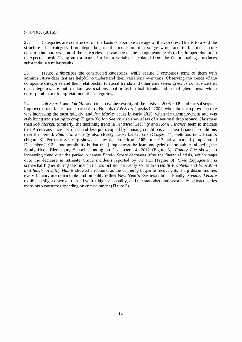
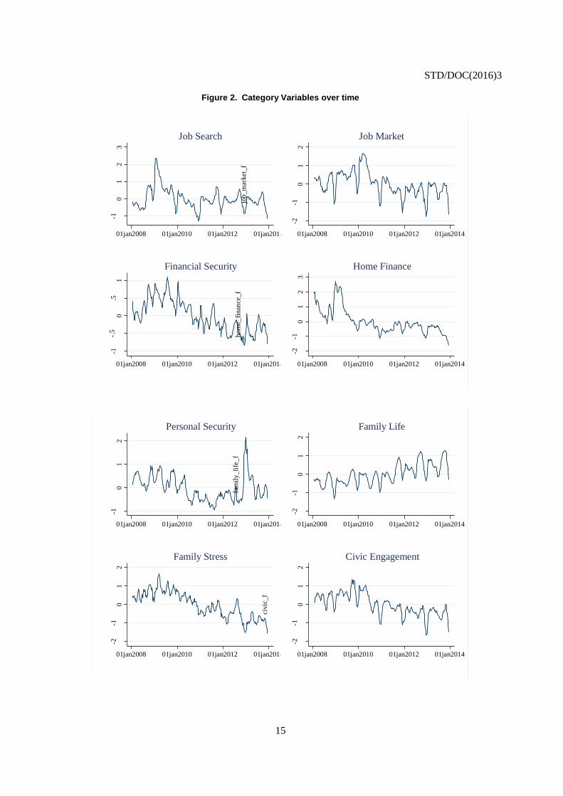
22. Categories are constructed on the basis of a simple average of the z-scores. This is to avoid the
structure of a category from depending on the inclusion of a single word, and to facilitate future
construction and revision of the categories, in case one of the components needs to be dropped due to an
unexpected peak. Using an estimate of a latent variable calculated from the factor loadings produces
substantially similar results.
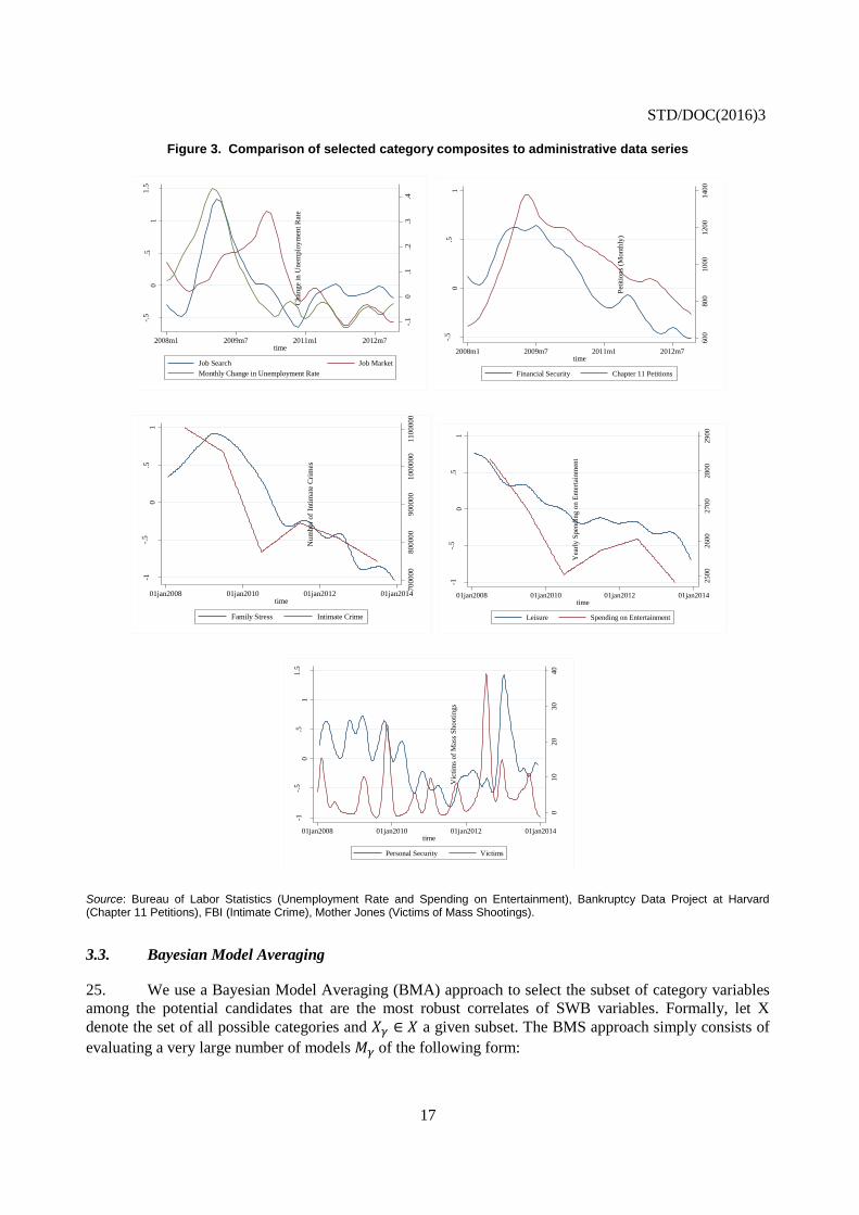
23. Figure 2 describes the constructed categories, while Figure 3 compares some of them with
administrative data that are helpful to understand their variations over time. Observing the trends of the
composite categories and their relationship to social trends and other data series gives us confidence that
our categories are not random associations, but reflect actual trends and social phenomena which
correspond to our interpretation of the categories.
24. Job Search and Job Market both show the severity of the crisis in 2008-2009 and the subsequent
improvement of labor market conditions. Note that Job Search peaks in 2009, when the unemployment rate
was increasing the most quickly, and Job Market peaks in early 2010, when the unemployment rate was
stabilizing and starting to drop (Figure 3); Job Search also shows less of a seasonal drop around Christmas
than Job Market. Similarly, the declining trend in Financial Security and Home Finance seem to indicate
that Americans have been less and less preoccupied by housing conditions and their financial conditions
over the period. Financial Security also closely tracks bankruptcy (Chapter 11) petitions in US courts
(Figure 3). Personal Security shows a slow decrease from 2009 to 2012 but a marked jump around
December 2012 – one possibility is that this jump shows the fears and grief of the public following the
Sandy Hook Elementary School shooting on December 14, 2012 (Figure 3). Family Life shows an
increasing trend over the period, whereas Family Stress decreases after the financial crisis, which maps
onto the decrease in Intimate Crime incidents reported by the FBI (Figure 3). Civic Engagement is
somewhat higher during the financial crisis but not markedly so, as are Health Problems and Education
and Ideals. Healthy Habits showed a rebound as the economy began to recover; its sharp discontinuities
every January are remarkable and probably reflect New Year’s Eve resolutions. Finally, Summer Leisure
exhibits a slight downward trend with a high seasonality, and the smoothed and seasonally adjusted series
maps onto consumer spending on entertainment (Figure 3).
STD/DOC(2016)3
15
Figure 2. Category Variables over time
-10
12
3
job
_se
arch
_f
01jan2008 01jan2010 01jan2012 01jan2014
Job Search
-2-1
01
2
job
_m
arket
_f
01jan2008 01jan2010 01jan2012 01jan2014
Job Market
-1-.
50
.51
fin
_se
curi
ty_f
01jan2008 01jan2010 01jan2012 01jan2014
Financial Security
-2-1
01
23
hom
e_fi
nan
ce_f
01jan2008 01jan2010 01jan2012 01jan2014
Home Finance
-10
12
per
sonal
_se
curi
ty_f
01jan2008 01jan2010 01jan2012 01jan2014
Personal Security
-2-1
01
2
fam
ily_
life
_f
01jan2008 01jan2010 01jan2012 01jan2014
Family Life
-2-1
01
2
fam
ily_
stre
ss_f
01jan2008 01jan2010 01jan2012 01jan2014
Family Stress
-2-1
01
2
civic
_f
01jan2008 01jan2010 01jan2012 01jan2014
Civic Engagement
STD/DOC(2016)3
16
-2-1
01
2
hea
lth_
con
dit
ion
s_f
01jan2008 01jan2010 01jan2012 01jan2014
Health Problems
-10
12
hea
lthy
_h
abit
s_f
01jan2008 01jan2010 01jan2012 01jan2014
Healthy Habits-2
-10
12
sum
mer
_le
isure
_f
01jan2008 01jan2010 01jan2012 01jan2014
Summer Leisure
-2-1
01
2
big
_p
ictu
re_f
01jan2008 01jan2010 01jan2012 01jan2014
Education and Ideals
STD/DOC(2016)3
17
Figure 3. Comparison of selected category composites to administrative data series
Source: Bureau of Labor Statistics (Unemployment Rate and Spending on Entertainment), Bankruptcy Data Project at Harvard (Chapter 11 Petitions), FBI (Intimate Crime), Mother Jones (Victims of Mass Shootings).
3.3. Bayesian Model Averaging
25. We use a Bayesian Model Averaging (BMA) approach to select the subset of category variables
among the potential candidates that are the most robust correlates of SWB variables. Formally, let X
denote the set of all possible categories and 𝑋𝛾 ∈ 𝑋 a given subset. The BMS approach simply consists of
evaluating a very large number of models 𝑀𝛾 of the following form:
-.1
0.1
.2.3
.4
Chan
ge
in U
nem
plo
ym
ent
Rat
e
-.5
0.5
11.5
2008m1 2009m7 2011m1 2012m7time
Job Search Job Market
Monthly Change in Unemployment Rate
60
08
00
10
00
12
00
14
00
Pet
itio
ns
(Mo
nth
ly)
-.5
0.5
1
Sta
nd
ard
ized
Cat
ego
ry S
earc
h F
req
uen
cy
2008m1 2009m7 2011m1 2012m7time
Financial Security Chapter 11 Petitions
70
00
00
80
00
00
90
00
00
10
00
00
01
10
00
00
Nu
mb
er o
f In
tim
ate
Cri
mes
-1-.
50
.51
01jan2008 01jan2010 01jan2012 01jan2014time
Family Stress Intimate Crime
25
00
26
00
27
00
28
00
29
00
Yea
rly
Sp
end
ing
on
En
tert
ain
men
t
-1-.
50
.51
Sta
nd
ard
ized
Cat
ego
ry S
earc
h F
req
uen
cy
01jan2008 01jan2010 01jan2012 01jan2014time
Leisure Spending on Entertainment
010
20
30
40
Vic
tim
s of
Mas
s S
hooti
ngs
-1-.
50
.51
1.5
Sta
ndar
diz
ed C
ateg
ory
Sea
rch F
requen
cy
01jan2008 01jan2010 01jan2012 01jan2014time
Personal Security Victims

STD/DOC(2016)3
18
𝑦 = 𝛼𝛾 + 𝛽𝛾𝑋𝛾 + 𝜀 𝜀 ~ 𝑁(0, 𝜎2𝐼)
with y being the SWB outcome, 𝛼𝛾 a constant, 𝛽𝛾 the coefficients and 𝜀 a normally distributed error
term of variance 𝜎2. As a matter of fact, most of SWB dependent variables surveyed by Gallup are
approximately normally distributed. Evaluating the model 𝑀𝛾 with regressors 𝑋𝛾 can be done through the
posterior model probability (PMP) which is from Bayes’ rule:
𝑃𝑀𝑃𝛾 = 𝑝(𝑀𝛾|𝑦, 𝑋) =𝑝(𝑦|𝑀𝛾 , 𝑋)𝑝(𝑀𝛾)
𝑝(𝑦|𝑋)
The quantity 𝑝(𝑦|𝑋) is independent of the model considered and can be viewed as a constant. As a
result, the PMP can be calculated as the model prior 𝑝(𝑀𝛾) times the conditional marginal likelihood
𝑝(𝑦|𝑀𝛾 , 𝑋). In a second step, these PMPs are used to infer the Posterior Inclusion Probability (PIP) of
each category variable, which is simply the sum of the PMPs of all models in which a given category
variable is included.5
3.4. Model Selection and Out-of-Sample Testing
26. Our methodology is designed to ensure that the weights on the categories used in the model do
not suffer from overfitting, spurious correlation, and constitute credible predictors of SWB variables. First,
we divide the sample into a “training” and “test” sample, and use the training sample to build the model,
and evaluate its performance on the test sample. Data from 2009 to 2013 are used for the training set, while
data from 2008 to 2009 are used for one test set and from 2013 to 2014 for the other. The reason for the
symmetrical test sets is that we would like to construct an index that predicts as well for periods of crises
(i.e. the 2008 economic crisis) as for periods of relative stability.
27. In practice, we first identify the most robust categories by applying BAM to the training data. All
categories with a PIP larger than 0.7 are pre-selected as a potential determinant of the SWB variable. The
PIPs of the various categories found in the exploratory analysis are reported in Annex C. On a second step,
we refine the model by simply regressing the dependent SWB variable on selected categories while using
the training dataset, and we remove any category with a non-significant coefficient. Finally, we use the
coefficients from the final model (estimated over the training period) to predict SWB over the whole
period, namely both training and test sub-periods. The next section evaluates how well the predictions fit
the actual data.
28. We intentionally exclude Home Finance from the model. While we recognize that financing a
home is an important life event for many Americans, the predominance of words related to home finance
(“mortgage”, for example) during this period is also critically linked to the financial crisis, and so the
importance of these words in predicting SWB is likely to be highly time-specific. As such, this category
5 We choose the model prior most commonly used in applied studies, namely the uniform distribution that assigns equal
prior probability 𝑝(𝑀𝛾) = 2−𝐾 to all 2𝐾 possible models. The use of the uniform model prior was first suggested by
Raftery (1988) while Hoeting et al. (1999) reviewed the evidence supporting the good performance of the uniform
model prior. It should be noted BMA does not compute the marginal likelihood and the posterior distribution for each
possible model. Instead, it identifies the subset of models where the mass of the model posterior probability is
concentrated. This is achieved with the help of a Metropolis-Hastings algorithm that walks randomly through the
model space but visits its most important part. In practice, we use the “birth-death” sampler that randomly chooses one
of the K variables at each step of the algorithm, and excludes it from the model if it is already included in it, or includes
it otherwise.

STD/DOC(2016)3
19
might dominate the prediction in the training data, and risk yielding poor results in the out of sample tests,
and having poor power to extrapolate to the future.
4. How to Google Subjective Well-Being in the United States?
4.1. A Model of SWB in the United States
29. Table 2 presents the results from the selected regression model for each SWB variable.6 The
coefficients are generally consistent for positive and negative affects. Categories that are consistently
associated with higher subjective well-being (excluding the Learn and Respect SWB variables, for which
our model does not perform well, as discussed below) are Job Market, Civic Engagement, Healthy Habits,
Summer Leisure, and Education and Ideals. Categories that are consistently associated with lower
subjective well-being are Job Search, Financial Security, Health Conditions, and Family Stress.
6 The dependent and explanatory variables have been standardized to allow for a comparison of the magnitude of the
effects at stake.

STD/DOC(2016)3
20
Table 2. Regression of Categories on Subjective Well-Being Data
30. Overall, these findings are in line with the literature on subjective well-being. The consistent
negative relationship of Job Search (which, as discussed above, seems to relate to searching for a job from
unemployment) confirms the importance of employment as a foundation of subjective well-being: having a
job is one of the strongest correlates of life satisfaction and happiness while, conversely, being unemployed
is highly detrimental to life satisfaction, beyond the loss of income that this entails (see, for example, Clark
and Oswald, 1994), and is most difficult to adapt to (Clark et al. 2008). There is evidence that objective
health shocks (such as heart attacks) are negatively correlated with SWB (Shields and Wheatley Price,
2005), though this relationship is more difficult to disentangle with confidence as reported health status
may be a proxy of subjective well-being and as such are highly correlated (Deaton, 2008). In addition,
there is evidence that higher levels of subjective well-being themselves lead to better health outcomes
(Howell et al, 2007).
31. Civic Engagement is related to the importance of social capital, which has been amply
demonstrated to be strongly associated with subjective well-being (Helliwell and Wang, 2011; Helliwell et
Life
Evaluation
Life
Evaluation
5 Years
Happiness Laugh Learn Respect Anger Stress Worry Sadness
(1) (2) (3) (4) (5) (6) (7) (8) (9) (10)
Material conditions
Job Search -0.772*** -0.293*** -0.466*** -0.452*** 0.571*** 0.387*** 0.751*** 0.619***
(0.075) (0.058) (0.061) (0.070) (0.067) (0.051) (0.042) (0.069)
Job Market 0.552*** 0.294** -0.297*** 1.261***
(0.121) (0.145) (0.101) (0.150)
Financial Security -0.327*** -0.712*** -0.596*** -0.481*** -0.415*** -0.657*** 1.234*** 0.402*** 0.438*** 0.440***
(0.112) (0.066) (0.114) (0.079) (0.088) (0.110) (0.180) (0.078) (0.057) (0.109)
Social
Family Life 0.251*** 0.266*** 0.403*** 0.416*** 0.478*** -0.367***
(0.080) (0.065) (0.057) (0.082) (0.049) (0.077)
Family Stress -0.381*** -0.269***
(0.091) (0.096)
Civic Engagement 0.477*** -0.182**
(0.115) (0.088)
Personal Security 0.199*** -0.410*** -0.266*** 0.282***
(0.049) (0.067) (0.055) (0.049)
Health and Wellness
Healthy Habits 0.203** 0.785*** 0.460*** 0.551*** 0.267*** -0.203* -0.373*** -0.402*** -0.280***
(0.079) (0.076) (0.103) (0.059) (0.066) (0.110) (0.057) (0.048) (0.078)
Summer Leisure -1.521*** -0.881*** -0.786*** -0.906***
(0.308) (0.143) (0.135) (0.212)
Health Conditions 0.478*** 0.262**
(0.113) (0.116)
Education and Ideals -1.092*** -0.393*** -0.654***
(0.182) (0.139) (0.150)
Month dummies Yes Yes Yes Yes Yes Yes Yes Yes Yes Yes
N 200 200 200 200 200 200 200 200 200 200
R2 0.798 0.652 0.688 0.828 0.861 0.662 0.606 0.904 0.868 0.816
Adj. R2 0.770 0.614 0.650 0.806 0.843 0.623 0.557 0.890 0.853 0.791
Positive Affects Negative Affects
note: Robust standard errors in parentheses, *** p<0.01, ** p<0.05, * p<0.1. Week dummies included for weeks in December and January,
month dummies included for all other months.
STD/DOC(2016)3
21
al., 2010). Healthy Habits, notably physical exercise, are associated with less depression and anxiety and
improved mood (Biddle and Ekkekakis, 2005). Education and Ideals is a grouping of words that includes
references to religion, political goals, philosophy, and education, and which is associated with higher
SWB, consistent with the literature that finds higher subjective well-being associated with religious
activity (Clark and Lelkes, 2005; Helliwell, 2003). Finally, family, health and security are identified,
through choices, as extremely important in terms of people’s happiness by Benjamin et al. (2014) and these
categories coincide with the “satisfaction domains” that have been explored by the Leyden school (van
Praag and Ferrer-i-Carbonell, 2008). Many of these patterns of subjective well-being are summarized in
The World Happiness Report (Helliwell et al., 2013, 2015).
32. Two categories have inconsistent signs. Family Life is associated with more Happiness and
Laughter, and less Sadness, but also with more Anger and Stress. (The finding of inconsistent associations
of Family Life may reflect the complicated nature of interactions with children, consistent with the finding
in Deaton and Stone (2014) that parents experience both more daily joy and more daily stress than non-
parents: see also Buddelmeyer et al., 2015.) Personal Security is positively associated with Life Evaluation
(today), but negatively associated with Life Evaluation in 5 years and Laughter, and positively associated
with Sadness. We cannot explain this difference. 7
33. These associations remain silent on causality since the different dimensions could be correlated
to each other or related to an omitted variable. Nevertheless, bearing this caveat in mind, we generally
observe that material condition aspects play an important role in our model, with job search and financial
security showing large, highly significant and consistent associations with almost all of the subjective well-
being categories. Job Search has the largest coefficient for all of the categories for Life Evaluation and
Worry; Financial Security has the largest coefficient for Life Evaluation in 5 years, Happiness, Laugh,
Learn and Anger, and is close to the largest for Respect and Sadness.
34. Social aspects play a large role in predicting Life Evaluation and other positive affects, though
the coefficients tend to be relatively smaller than the Material Conditions aspects. Health and Wellness
aspects are most significant with respect to predicting negative affects, with the exception of Healthy
Habits, which is consistently significant for every affect except Anger. Note also that Healthy Habits has a
relatively large coefficient with respect to Life Evaluation in 5 years. Summer Leisure is consistently
associated with lower negative affects but not with higher positive affects, and the largest coefficient is
associated with reduced Anger.
4.2. Variance Decomposition
35. Simple variance decomposition can help to quantify the contributions of each covariate to the R2.
It simply follows from the equality:
7 Note that, generally, living in a high crime area is associated with lower SWB as argued by Lelkes, 2006.
i
RtooncontributiX
j
jiji
j
jj
i
ii
i
ii
i
XXCovXXCovXVarR
2
),(,2
STD/DOC(2016)3
22
Note that some contributions can be negative if the covariance terms are larger than the individual
variance of variable Xi and are negative. This case typically occurs when a given variable is highly
correlated with others but has the opposite sign.
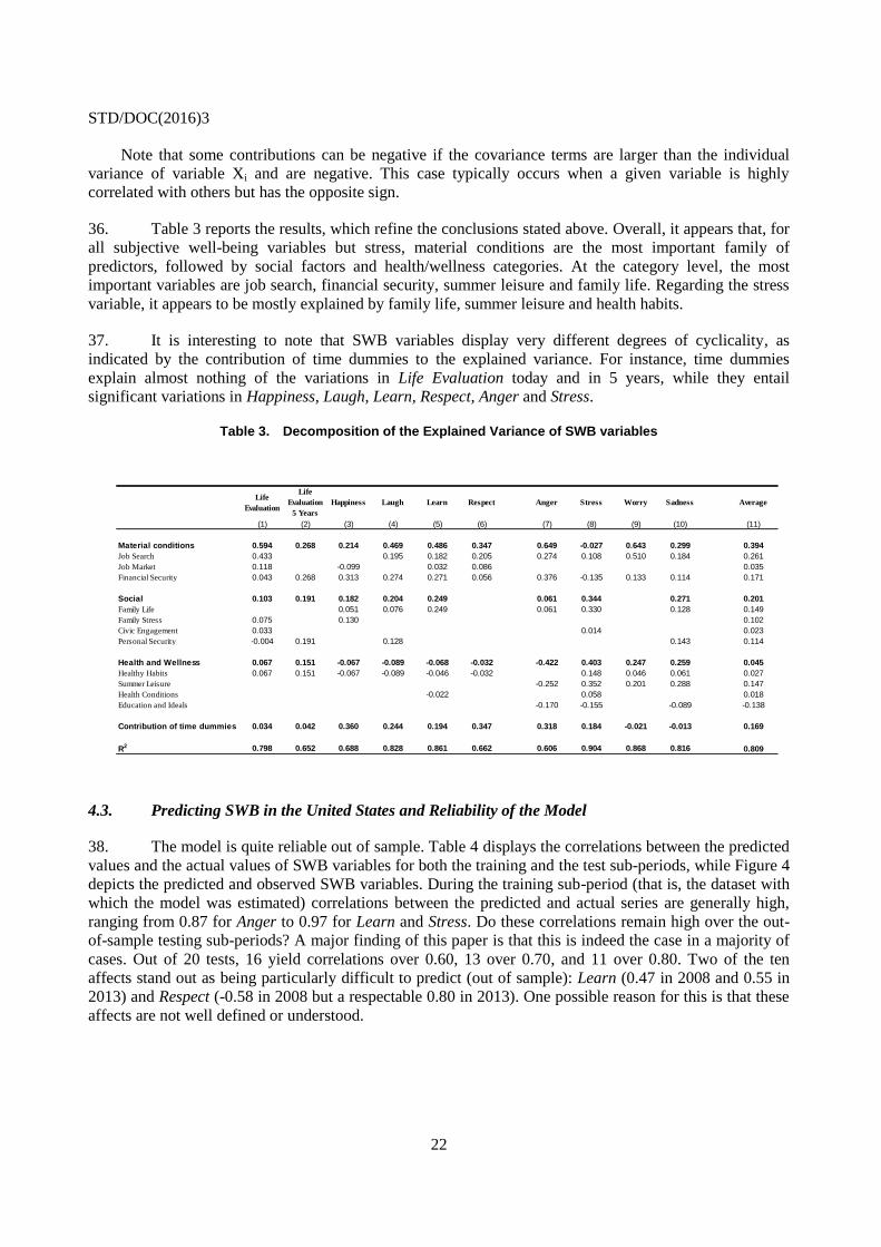
36. Table 3 reports the results, which refine the conclusions stated above. Overall, it appears that, for
all subjective well-being variables but stress, material conditions are the most important family of
predictors, followed by social factors and health/wellness categories. At the category level, the most
important variables are job search, financial security, summer leisure and family life. Regarding the stress
variable, it appears to be mostly explained by family life, summer leisure and health habits.
37. It is interesting to note that SWB variables display very different degrees of cyclicality, as
indicated by the contribution of time dummies to the explained variance. For instance, time dummies
explain almost nothing of the variations in Life Evaluation today and in 5 years, while they entail
significant variations in Happiness, Laugh, Learn, Respect, Anger and Stress.
Table 3. Decomposition of the Explained Variance of SWB variables
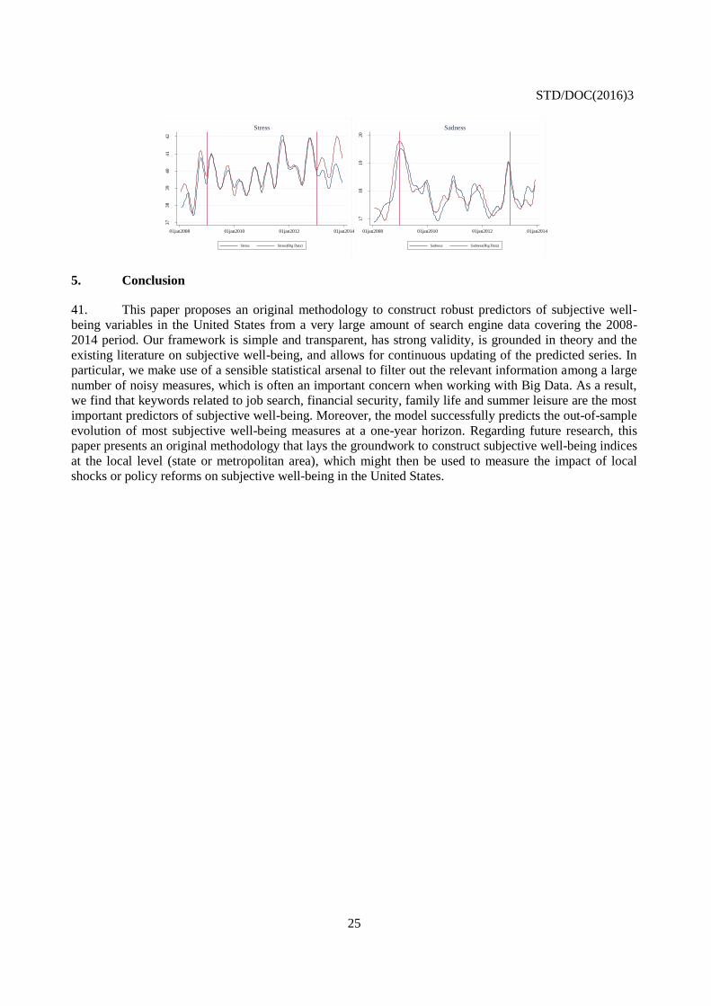
4.3. Predicting SWB in the United States and Reliability of the Model
38. The model is quite reliable out of sample. Table 4 displays the correlations between the predicted
values and the actual values of SWB variables for both the training and the test sub-periods, while Figure 4
depicts the predicted and observed SWB variables. During the training sub-period (that is, the dataset with
which the model was estimated) correlations between the predicted and actual series are generally high,
ranging from 0.87 for Anger to 0.97 for Learn and Stress. Do these correlations remain high over the out-
of-sample testing sub-periods? A major finding of this paper is that this is indeed the case in a majority of
cases. Out of 20 tests, 16 yield correlations over 0.60, 13 over 0.70, and 11 over 0.80. Two of the ten
affects stand out as being particularly difficult to predict (out of sample): Learn (0.47 in 2008 and 0.55 in
2013) and Respect (-0.58 in 2008 but a respectable 0.80 in 2013). One possible reason for this is that these
affects are not well defined or understood.
Life
Evaluation
Life
Evaluation
5 Years
Happiness Laugh Learn Respect Anger Stress Worry Sadness Average
(1) (2) (3) (4) (5) (6) (7) (8) (9) (10) (11)
Material conditions 0.594 0.268 0.214 0.469 0.486 0.347 0.649 -0.027 0.643 0.299 0.394
Job Search 0.433 0.195 0.182 0.205 0.274 0.108 0.510 0.184 0.261
Job Market 0.118 -0.099 0.032 0.086 0.035
Financial Security 0.043 0.268 0.313 0.274 0.271 0.056 0.376 -0.135 0.133 0.114 0.171
Social 0.103 0.191 0.182 0.204 0.249 0.061 0.344 0.271 0.201
Family Life 0.051 0.076 0.249 0.061 0.330 0.128 0.149
Family Stress 0.075 0.130 0.102
Civic Engagement 0.033 0.014 0.023
Personal Security -0.004 0.191 0.128 0.143 0.114
Health and Wellness 0.067 0.151 -0.067 -0.089 -0.068 -0.032 -0.422 0.403 0.247 0.259 0.045
Healthy Habits 0.067 0.151 -0.067 -0.089 -0.046 -0.032 0.148 0.046 0.061 0.027
Summer Leisure -0.252 0.352 0.201 0.288 0.147
Health Conditions -0.022 0.058 0.018
Education and Ideals -0.170 -0.155 -0.089 -0.138
Contribution of time dummies 0.034 0.042 0.360 0.244 0.194 0.347 0.318 0.184 -0.021 -0.013 0.169
R2 0.798 0.652 0.688 0.828 0.861 0.662 0.606 0.904 0.868 0.816 0.809

STD/DOC(2016)3
23
Table 4. Correlation between Predicted and Observed SWB values (Smoothed)
Life
Evaluation
Life
Evaluation
5 Years Happiness Laugh Learn Respect Anger Stress Worry Sadness
Training 0.93 0.87 0.90 0.96 0.96 0.92 0.91 0.97 0.96 0.94
Test 2008 0.85 0.76 0.63 0.85 0.47 -0.58 0.60 0.92 0.94 0.89
Test 2014 0.92 0.86 0.47 0.86 0.55 0.80 0.61 0.82 0.84 0.70
39. In the case of Life evaluation this may be due to the change in the ordering of questions in the
Gallup survey that took place at about this time, and is thought to depress the overall Life evaluation
measure, as reported by Deaton (2011).
40. However, the objective of this exercise is to obtain a combination of keywords that is able to
predict the evolution — rather than the level — of subjective well-being, both cognitive and emotional.
With respect to this objective, it seems that such an exercise is not out of reach, at least over a 12 month
period. Big Data creates a new avenue for constructing a high-frequency indicator of subjective well-being
beyond GDP

STD/DOC(2016)3
24
Figure 4. Predictions and Observed SWB (Training Data inside the red lines, Test Data outside)
6.6
6.7
6.8
6.9
7
01jan2008 01jan2010 01jan2012 01jan2014
Life Evaluation Life Evaluation (Big Data)
Life Evaluation
7.5
7.6
7.7
7.8
01jan2008 01jan2010 01jan2012 01jan2014
Life Evaluation 5 years Life Evaluation 5 years (Big Data)
Life Evaluation 5 years
87
87.5
88
88.5
89
01jan2008 01jan2010 01jan2012 01jan2014
Happiness Happiness(Big Data)
Happiness
80
81
82
83
01jan2008 01jan2010 01jan2012 01jan2014
Laugh Laugh(Big Data)
Laugh
91
91.5
92
92.5
01jan2008 01jan2010 01jan2012 01jan2014
Respect Respect(Big Data)
Respect
58
60
62
64
66
01jan2008 01jan2010 01jan2012 01jan2014
Learn Learn(Big Data)
Learn
30
32
34
36
01jan2008 01jan2010 01jan2012 01jan2014
Worry Worry(Big Data)
Worry
12.5
13
13.5
14
14.5
01jan2008 01jan2010 01jan2012 01jan2014
Anger Anger(Big Data)
Anger
STD/DOC(2016)3
25
5. Conclusion
41. This paper proposes an original methodology to construct robust predictors of subjective well-
being variables in the United States from a very large amount of search engine data covering the 2008-
2014 period. Our framework is simple and transparent, has strong validity, is grounded in theory and the
existing literature on subjective well-being, and allows for continuous updating of the predicted series. In
particular, we make use of a sensible statistical arsenal to filter out the relevant information among a large
number of noisy measures, which is often an important concern when working with Big Data. As a result,
we find that keywords related to job search, financial security, family life and summer leisure are the most
important predictors of subjective well-being. Moreover, the model successfully predicts the out-of-sample
evolution of most subjective well-being measures at a one-year horizon. Regarding future research, this
paper presents an original methodology that lays the groundwork to construct subjective well-being indices
at the local level (state or metropolitan area), which might then be used to measure the impact of local
shocks or policy reforms on subjective well-being in the United States.
37
38
39
40
41
42
01jan2008 01jan2010 01jan2012 01jan2014
Stress Stress(Big Data)
Stress
17
18
19
20
01jan2008 01jan2010 01jan2012 01jan2014
Sadness Sadness(Big Data)
Sadness
STD/DOC(2016)3
26
REFERENCES
Askitas, N. and K.F. Zimmermann (2010), “Google Econometrics and Unemployment Forecasting”,
Technical Report, SSRN 899, [Cited 1 April 2012], available from:
http://papers.ssrn.com/sol3/papers.cfm?abstract_id¼1465341
Baker, S. and A. Fradkin (2014), “The Impact of Unemployment Insurance on Job Search: Evidence from
Google Search Data”.
Benjamin D., O. Heffetz, M. Kimball and N. Szembrot (2014), “Beyond Happiness and Satisfaction:
Toward Well-Being Indices Based on Stated Preference”, American Economic Review, No. 104.9,
pp. 2698-2735.
Biddle, S.J., and P. Ekkekakis (2005), Physically active lifestyles and well-being, The science of well-
being, pp. 140-168.
Buddelmeyer H., D. Hamermesh and M. Wooden (2015), “The Stress Cost of Children”, IZA Discussion
Paper No. 8793.
Choi, H. and H. Varian (2009), “Predicting Initial Claims for Unemployment Insurance Using Google
Trends”, Technical report, Google, [Cited 1 April 2012], available from:
http://research.google.com/archive/papers/initialclaimsUS.pdf
Choi, H. and H. Varian (2012), “Predicting the Present with Google Trends”, The Economic Record,
Vol. 88, pp. 2-9.
Clark A. and A. Oswald (1994), “Unhappiness and Unemployment”, Economic Journal, No. 104, pp. 648-
659.
Clark A., E. Diener, Y. Georgellis and R. Lucas (2008), “Lags and Leads in Life Satisfaction: A Test of the
Baseline Hypothesis”, Economic Journal, Vol. 118, No. 529.
D’Amuri F. and J. Marcucci (2010), “Google it! Forecasting the US Unemployment Rate with a Google
Job Search Index”, Social Science Research Network, [Cited 1 April 2012], available from:
http://papers.ssrn.com/sol3/papers.cfm?abstract_id¼1594132
Deaton A. (2008), “Income, Health and Well-Being around the World: Evidence from the Gallup World
Poll”, Journal of Economic Perspectives, Vol. 22, No. 2, pp. 53-72.
Deaton A. (2011), “The Financial crisis and the well-being of Americans”, NBER WP No. 17128.
Deaton A. and A. Stone (2014), “Evaluative and hedonic wellbeing among those with and without children
at home”, Proceedings of the National Academy of Sciences, Vol. 111, No. 4, pp. 1328-1333.
Eicher T.S., C. Papageorgiou and A.E. Raftery (2011), “Default priors and predictive performance in
Bayesian model averaging, with application to growth determinants”, Journal of Applied
Econometrics, Vol. 26, No. 1, pp. 30-55.
STD/DOC(2016)3
27
Ettredge M., J. Gerdes and G. Karuga (2005), “Using Web-based Search Data to Predict Macroeconomic
Statistics”, Communications of the ACM, Vol. 48, No. 11, pp. 87-92, [Cited 1 April 2012], available
from: http://portal.acm.org/citation.cfm?id¼1096010
George D. and P. Mallery (2003), SPSS for Windows step by step: A simple guide and reference, 11.0
update (4th ed.), Boston: Allyn & Bacon.
Helliwell J. and S. Wang (2011), “Trust and Wellbeing”, International Journal of Wellbeing, Vol. 1,
pp. 42-78.
Helliwell J., C. Barrington-Leigh, A. Harris and H. Huang (2010), “International Evidence on the Social
Context of Well-Being”, in Diener E., Helliwell J. and Kahneman D. (eds.), International
Differences in Well-Being, Oxford University Press.
Helliwell J., R. Layard and J. Sachs (2015), World Happiness Report, United Nations.
Hoeting J.A., D. Madigan, A.E. Raftery and C.T. Volinsky (1999), “Bayesian Model Averaging: A
Tutorial”, Statistical Science 14, pp. 382-417.
Howell R.T., M.L. Kern and S. Lyubomirsky (2007), “Health benefits: Meta-analytically determining the
impact of well-being on objective health outcomes”, Health Psychology Review, Vol. 1, No. 1,
pp. 83-136.
Kahneman D. and A. Deaton (2010), High income improves evaluation of life but not emotional well-
being, Proceedings of the national academy of sciences, Vol. 107, No. 38, pp. 16489-16493.
Lelkes O. (2006), Knowing what is good for you: Empirical analysis of personal preferences and the
“objective good”, The Journal of Socio-Economics, 35 (2), pp. 285-307.
Mavridis D. (2015), “The unhappily unemployed return to work faster”, IZA Journal of Labor Economics,
Vol. 4, No. 1, pp. 1-22.
Nunnally J.C. (1978), “Assessment of Reliability”, in Psychometric Theory (2nd ed.), New York:
McGraw-Hill.
OECD (2013), OECD Guidelines on Measuring Subjective Well-being, OECD Publishing, Paris,
DOI: http://dx.doi.org/10.1787/9789264191655-en
Penna N.D. and H. Huang (2009), “Constructing Consumer Sentiment Index for U.S. Using Google
Searches”, Technical report, University of Alberta, [Cited 1 April 2012], available from:
http://econpapers.repec.org/paper/risalbaec/2009_5f026.htm
Preis T., D. Reith and H. Eugene Stanley (2010), “Complex Dynamics of Our Economic Life on Different
Scales: Insights from Search Engine Query Data”, Philosophical.
Radinsky K., S. Davidovich and S. Markovitch (2009), “Predicting the News of Tomorrow Using Patterns
in Web Search Queries”, Proceedings of the 2008 IEEE/WIC/ACM International Conference on
Web Intelligence (WI08), [Cited 1 April 2012], available from:
http://www.cs.technion.ac.il/~shaulm/papers/pdf/Radinsky-WI2008.pdf
Raftery A.E. (1988), “Approximate Bayes Factors for Generalized Linear Models”, Technical Report
No. 121, Department of Statistics, University of Washington.

STD/DOC(2016)3
28
Reimsbach-Kounatze, C. (2015), “The Proliferation of ‘Big Data’ and Implications for Official Statistics
and Statistical Agencies: A Preliminary Analysis”, OECD Digital Economy Papers, No. 245, OECD
Publishing.
Schwartz H.A., J.C. Eichstaedt, M.L. Kern, L. Dziurzynski, M. Agrawal, G.J. Park, S.K. LakshmikanthJha,
M.E.P. Seligman, L. Ungar and R.E. Lucas (2013), “Characterizing Geographic Variation in Well-
Being using Tweets”, Proceedings of the Association for the Advancement of Artificial Intelligence.
Scott S.L. and H.R. Varian (2012), “Bayesian Variable Selection for Nowcasting Economic Time Series”.
Scott S.L. and H.R. Varian (2014), “Predicting the present with Bayesian structural time series”,
International Journal of Mathematical Modelling and Numerical Optimisation, Vol. 5, No. 1/2,
pp. 4-23
Shields M.A. and S.W. Price (2005), “Exploring the economic and social determinants of psychological
well‐being and perceived social support in England”, Journal of the Royal Statistical Society: Series
A (Statistics in Society), Vol. 168, No. 3, pp. 513-537.
Stiglitz J., A. Sen and J.P. Fitoussi (2009), Rapport de la Commission sur la mesure des performances
économiques et du progrès social, France.
Steptoe, A., Deaton A. and A.A. Stone (2014), “Subjective Wellbeing, Health, and Ageing”, The Lancet,
Vol. 385, No. 9968, pp. 640-648.
Suhoy T. (2009), “Query Indices and a 2008 Downturn: Israeli Data”, Technical report, Bank of Israel,
[Cited 1 April 2012], available from:
http://www.bankisrael.gov.il/deptdata/mehkar/papers/dp0906e.pdf
Transactions of the Royal Society of London, pp. 5707-19, [Cited 1 April 2012], available from:
http://rsta.royalsocietypublishing.org/content/368/1933/5707
Van Praag B. and A. Ferrer-I-Carbonell eds. (2008), Happiness Quantified: A Satisfaction Calculus
Approach, Oxford University Press.

STD/DOC(2016)3
29
APPENDIX A. BIG DATA ISSUES
This Appendix gives additional detail on problems encountered with the data on search volume
downloaded from Google Trends. There are four main types of problems: spikes, cliffs, the January 2011
discontinuity, and time trends.
Spikes
Many search terms show large spikes. These spikes might either be related to the importance of
the underlying word, related to a tangential cultural event, or be unexplained. The spikes pose two different
problems. The first problem is that if they are unrelated to the underlying concept of interest (see, for
example, Figure A1, showing the divorce of Kim Kardashian, an American celebrity as the likely cause of
the spike in searches that include the term “divorce” during the last week of October, 2011), they will add a
large amount of statistical noise. The second is that even if they are related to the underlying concept, they
will lead to large outliers in the explanatory variables. If a sufficient number of explanatory variables have
such outliers, the risk of overfitting increases (in principal, if there are as many explanatory variables with
spikes as there are data points, one could fit the series perfectly). We address this problem in two ways.
First, we use a five-period moving average in the analysis, which dampens shocks within an individual
keyword. Second, the composite indicators dampen the shock present across keywords.
Figure A1. “Spikes” and the Divorce of Kim Kardashian
20
40
60
80
100
div
orc
e
01jan2008 01jan2010 01jan2012 01jan2014time
Divorce
October 31, 2011: Kim Kardashian files
for divorce from Kris Humphries after
72 days of marriage

STD/DOC(2016)3
30
Cliffs
Other search terms show “cliffs”, where volume is at or near zero for some substantial period
(see Figure A2 below), and it is difficult to know whether it is because volume was zero or because there is
an issue with the way the Google trends data is compiled. These cliffs pose an issue similar to that of the
spikes, especially since words have cliffs at different points (that is, it is into a uniform discontinuity).
However, we do not wish to exclude all zeros, because some zeros reflect zero volume. To address this
issue, we dropped any search term with more than five zeros during the period (changing the number of
allowable zeros does not substantially change the results). This results in a loss of information, as we have
to exclude many terms that are potentially salient and important (such as mace spray).
Figure A2. “Cliffs” and Mace Spray
The January 2011 Discontinuity
We observed an unexplained discontinuity in many search term volumes from the last week of
December, 2010, to the first week of January, 2011. An example for the word “pregnancy” is provided in
Figure A3. To adjust for this discontinuity, which we believe to be related to the localization used by
Google in treating the data, we calculate the average index in December and January for the unaffected
years, we take the average change during the unaffected years, subtract this unaffected average change
from the observed change from December 2010 to January 2011, and adjust all data from 2011 onwards
using this difference. That is, we assume that the change from December 2010 to January 2011 should be
the same as in the other years, and we adjust accordingly. While we may lose some information with this
adjustment, there should not be any bias introduced.
020
40
60
80
100
mac
e sp
ray
01jan2008 01jan2010 01jan2012 01jan2014time
Mace Spray

STD/DOC(2016)3
31
Figure A3. Adjustment for the January 2011 Discontinuity
Time Trends
Some search terms (see “teeth hurt” in Figure A4) exhibit strong time trends. There are several
possibilities for this. First, it may be that the importance of this term is increasing – that is, either people
have more tooth pain or it bothers them more, and that this trend continued fairly consistently for six years.
Second, it may be that people experience the same amount of discomfort from tooth pain, but they are
turning more and more to the internet for advice on this type of problem (either because of cultural shifts or
external factors such as increasing health care costs). There might also be a third reason related to the
compilation of the search data within Google that we do not know. The time trends are problematic for at
least two reasons. First, a positive coefficient on a term with a strong time trend might lead to large and
unrealistic predictions for subjective well-being in the future. Second, as our estimation strategy relies on
creating statistically coherent composite variables, we risk grouping together words that are unrelated but
share a common time trend. To avoid these issues we drop all words where the adjusted R2 (using training
data only) from a regression of time on the keyword is greater than 0.6, and we individually examine the
series for words between 0.5 and 0.6 and drop the word if the trend is consistent over the period.
Figure A4. Time trends in “Teeth hurt”
70
80
90
100
pre
gnan
cy
01jan2008 01jan2010 01jan2012 01jan2014time
Pregnancy -unadjusted
60
70
80
90
100
pre
gnan
cy
01jan2008 01jan2010 01jan2012 01jan2014time
Pregnancy -adjusted
20
40
60
80
100
teet
h h
urt
01jan2008 01jan2010 01jan2012 01jan2014time
Teeth Hurt

STD/DOC(2016)3
32
APPENDIX B. EXPLORATORY FACTOR ANALYSIS
To group the search terms into coherent categories, we took the following steps. First, we
removed seasonality by regressing month and, for January and December, week dummies on the search
volume, to avoid grouping terms together only because they shared seasonal patterns. Second, we roughly
grouped the words into a priori related categories (such as jobs or family). Third, we ran a factor analysis,
removing any terms which had a factor loading of less than 0.3. These removed terms might also form a
separate category (so jobs was divided into Job Search and Job Market). The factor loadings from the final
categories are given below. In order to preserve the option of future application of the categories, we use a
z-score average to compute the actual category rather than the factor loadings. Using the factors rather than
the z-score averages produces almost identical results.
Table B1. Factor Loading for Material Conditions Variables
Job Search Factor Loadings
Job Market Factor Loadings
Financial Security
Factor Loadings
Home Finance Factor Loadings
part time job 0,734 jobbenefits 0,528 401K 0,478 mortgage rates 0,962
layoffs 0,879 employment contract
0,864 banking 0,790 mortgage calculator
0,913
jobfair 0,874 careercenter 0,871 family budget 0,374 mortgage 0,995
apprenticeships 0,825 coverletter 0,888 housing authority
0,712 refinancing 0,934
severance pay 0,817 pension 0,557 section8 0,500 houseprice 0,780
unemployment rate
0,798 cert prog 0,482 inflation 0,770 homeloan 0,927
careerfair 0,626 retirement 0,901 studentloans 0,764 housing crisis 0,849
jobs 0,408 work experience 0,568 school loans 0,858 mortgage payments
0,764
unemployment benefits
0,473 entrylevel 0,755 interestrate 0,839
qualifications 0,905 fired 0,562
discrimination 0,806 financial crisis 0,782
employee benefits
0,903 loans 0,954
eitc 0,837
socialsecurity 0,692
coupons 0,492
medicaid 0,413
file for bankruptcy
0,622
shelter 0,726
eviction 0,623
foodbank 0,755
homelessshelters 0,716

STD/DOC(2016)3
33
Table B2. Factor Loading for Social Variables
Family Stress Factor Loadings
Family Time Factor Loadings
Civic Engagement
Factor Loadings
Personal Security Factor Loadings
domestic abuse
0,889 snacksforkids 0,821 volunteering 0,855 firearm 0,845
marriagehelp 0,763 weekends 0,380 blood donation 0,656 victims 0,771
marriage problems
0,776 adhd 0,558 homeowners association
0,817 gun 0,728
custody 0,690 daycare 0,543 boyscouts 0,645 gunsafety 0,754
marriage counseling
0,822 child care center 0,555 kiwanis 0,920 violent crimes 0,858
familysupport 0,870 pta 0,758 citycouncil 0,767 crime rate 0,870
womensshelter 0,432 kidsparty 0,402 freemasons 0,642 assault 0,647
volleyball 0,359 bingo 0,548 securitycamera 0,558
play football 0,792 teaparty 0,496 murder 0,481
reading 0,470 lionsclub 0,653 selfdefense 0,552
recipe 0,602 club 0,779 aggression 0,303
housework 0,397 community meeting
0,439 risks 0,245
laundry 0,820 civic engagement
0,364 homealarm 0,246
toddler 0,810 rotaryclub 0,889 mugging 0,314
babyshower 0,820 towncouncil 0,559
bullying 0,637
kids books 0,881
ideasforkids 0,919
tuition 0,782
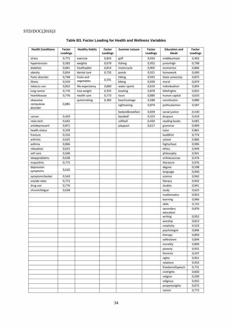
STD/DOC(2016)3
34
Table B3. Factor Loading for Health and Wellness Variables
Health Conditions Factor Loadings
Healthy Habits Factor Loadings
Summer Leisure Factor Loadings
Education and Ideals
Factor Loadings
stress 0,772 exercise 0,824 golf 0,934 middleschool 0,493
hypertension 0,583 weights 0,679 fishing 0,952 juniorhigh 0,798
diabetes 0,841 healthydiet 0,814 motorcycle 0,905 economics 0,866
obesity 0,834 dental care 0,735 ponds 0,921 homework 0,690
Panic disorder 0,748 fruits and vegetables 0,591
hiking 0,925 State university 0,872
illness 0,559 biking 0,939 moral 0,879
tobacco use 0,832 life expectancy 0,800 water sports 0,610 individualism 0,893
lung cancer 0,776 lose weight 0,355 boating 0,878 billofrights 0,825
heartdisease 0,776 health care 0,773 tours 0,880 human capital 0,633
obsessive compulsive disorder
0,885 quitsmoking 0,383 beachcottage 0,588 constitution 0,880
sightseeing 0,874 politicalaction 0,587
bedandbreakfast 0,839 social justice 0,530
cancer 0,429 baseball 0,323 dropout 0,419
relax tech 0,642 softball 0,420 reading books 0,681
antidepressant 0,871 playpool 0,617 grammar 0,909
health status 0,339 tutor 0,861
fracture 0,316 buddhist 0,774
arthritis 0,625 school 0,866
asthma 0,866 highschool 0,906
relaxation 0,615 ethics 0,944
self care 0,506 philosophy 0,941
sleepproblems 0,638 onlinecourses 0,476
mayoclinic 0,775 literature 0,976
depression symptoms 0,620
degree 0,598
language 0,940
symptomchecker 0,543 science 0,942
suicide rates 0,772 literacy 0,942
drug use 0,776 studies 0,941
chronicfatigue 0,638 study 0,625
mathematics 0,953
learning 0,966
skills 0,725
secondary education
0,876
writing 0,952
worship 0,812
creativity 0,523
psychologist 0,896
therapy 0,850
selfesteem 0,894
morality 0,809
poverty 0,931
feminist 0,547
rights 0,951
relations 0,933
freedomofspeech 0,731
civilrights 0,830
religion 0,509
religious 0,932
propertyrights 0,672
racism 0,772

STD/DOC(2016)3
35
governments 0,361
freespeech 0,775
rituals 0,850
infant mortality 0,837
spirituality 0,802

STD/DOC(2016)3
36
APPENDIX C. BAYESIAN AVERAGING MODEL RESULTS
Life Evaluation Life Evaluation in 5 Years Happiness Laugh Learn
Category PIP Category PIP Category PIP Category PIP Category PIP
Job Search 1 Family Stress .9999999 Family Life .9999308 Job Search 1 Job Search 1
Family Stress .9999345 Financial Security .9999994 Job Market .9988018 Family Life 1 Family Life .9999999
Job Market .9959486 Job Search .9987293 Financial Security .9612713 Personal Security .9987682 Health Conditions .9926389
Healthy Habits .9756049 Personal Security .9867251 Job Search .7824603 Summer Leisure .9339863 Financial Security .9868134
Civic Engagement .896345 Job Market .9126053 Summer Leisure .5180083 Health Conditions .9287642 Healthy Habits .8700904
Financial Security .4405012 Family Life .7997323 Education and Ideals .3740062 Financial Security .7978849 Job Market .7783921
Summer Leisure .0798991 Education and Ideals .1033073 Family Stress .2125029 Civic Engagement .5212126 Family Stress .2353987
Civic Engagement .0968726 Civic Engagement .1982485 Job Market .4633149 Summer Leisure .136816
Summer Leisure .0882474 Health Conditions .0954218 Family Stress .1317561 Education and Ideals .0983368
Health Conditions .0730709 Personal Security .0713978 Education and Ideals .1096197 Civic Engagement .0924329
Personal Security .0689583
Respect Anger Stress Worry Sadness
Category PIP Category PIP Category PIP Category PIP Category PIP
Job Market 1 Job Search 1 Family Life 1 Job Search 1 Job Search 1
Job Search .9999644 Financial Security .9999973 Job Search 1 Summer Leisure .9999992 Personal Security .9999999
Financial Security .9995359 Summer Leisure .9999353 Healthy Habits .9999991 Healthy Habits .9999803 Family Life .9998972
Healthy Habits .2881511 Education and Ideals .9795223 Summer Leisure .9999747 Financial Security .9998447 Summer Leisure .9981101
Personal Security .1305427 Civic Engagement .0981886 Financial Security .9726784 Family Stress .6311848 Education and Ideals .9921088
Family Stress .1250909 Health Conditions .0951104 Education and Ideals .7365542 Education and Ideals .5506082 Financial Security .9878952
Summer Leisure .0748373 Job Market .0887169 Civic Engagement .4862978 Health Conditions .5280867 Healthy Habits .9852301
Personal Security .0664031 Health Conditions .3005131 Personal Security .5102105 Health Conditions .1115238
Family Stress .0663557 Family Stress .2364499 Civic Engagement .0752305 Civic Engagement .0924093
Personal Security .1218278 Family Life .067823 Family Stress .0690964
Job Market .0749033
Output from Bayesian Model Selection routine carried out in R using BMS package, with 1M iterations. Fixed effects were included for weeks during the months of December and January, and months during the rest of the year. PIP indicates the posterior inclusion probability. To avoid overfitting, the categories used for each SWB variable were restricted to those that increased the adjusted R2 when included in
a regression with month and week controls.

STD/DOC(2016)3
37