unclassified delsa/elsa/wd/sem(2009)18
TRANSCRIPT

Unclassified DELSA/ELSA/WD/SEM(2009)18 Organisation de Coopération et de Développement Économiques Organisation for Economic Co-operation and Development 20-Aug-2009
___________________________________________________________________________________________
_____________ English - Or. English DIRECTORATE FOR EMPLOYMENT, LABOUR AND SOCIAL AFFAIRS
EMPLOYMENT, LABOUR AND SOCIAL AFFAIRS COMMITTEE
OECD SOCIAL, EMPLOYMENT AND MIGRATION WORKING PAPERS No. 90
GOING SEPARATE WAYS? SCHOOL-TO-WORK TRANSITIONS IN THE UNITED STATES AND
EUROPE
Glenda Quintini and Thomas Manfredi
JEL codes for classification: J21, J22, J64
JT03268726
Document complet disponible sur OLIS dans son format d'origine
Complete document available on OLIS in its original format
DE
LS
A/E
LS
A/W
D/S
EM
(2009)1
8
Un
classified
En
glish
- Or. E
ng
lish

DELSA/ELSA/WD/SEM(2009)18
2
DIRECTORATE FOR EMPLOYMENT, LABOUR AND SOCIAL AFFAIRS
http://www.oecd.org/els
OECD SOCIAL, EMPLOYMENT AND MIGRATION
WORKING PAPERS
http://www.oecd.org/els/workingpapers
This series is designed to make available to a wider readership selected labour market, social policy and
migration studies prepared for use within the OECD. Authorship is usually collective, but principal writers
are named. The papers are generally available only in their original language – English or French – with a
summary in the other.
Comment on the series is welcome, and should be sent to the Directorate for Employment, Labour and
Social Affairs, 2, rue André-Pascal, 75775 PARIS CEDEX 16, France.
The opinions expressed and arguments employed here are the responsibility
of the author(s) and do not necessarily reflect those of the OECD.
Applications for permission to reproduce or translate
all or part of this material should be made to:
Head of Publications Service
OECD
2, rue André-Pascal
75775 Paris, CEDEX 16
France
Copyright OECD 2009

DELSA/ELSA/WD/SEM(2009)18
3
ACKNOWLEDGEMENTS
Glenda Quintini is an economist in the Employment Analysis and Policies Division at the OECD
Directorate for Employment, Labour and Social Affairs and Thomas Manfredi is a statistician in the same
division. Comments, suggestions and advice from John P. Martin, Stefano Scarpetta and other OECD staff
are gratefully acknowledged. The views expressed in this paper are those of the authors and do not
necessarily reflect those of the OECD or of its member countries.

DELSA/ELSA/WD/SEM(2009)18
4
SUMMARY
This paper derives school-to-work transition pathways in the United States and Europe between the
late 1990s and the early 2000s. To do so, it uses Optimal Matching, a technique developed to sequence
DNA. The key advantage of using this technique is that, rather than focusing on a specific point in time or
a single destination, such as employment, inactivity or unemployment, they convey information on all
activities undertaken by youth over the transition period, their sequence and their persistence. Strong
similarities are found between the United States and Europe. However, pathways in the United States are
characterised by significantly more dynamism than in Europe: youth in employment tend to change jobs
more frequently while inactive or unemployed youth are more likely to experience several short spells
rather than a single long one. School-to-work transition pathways in the United States also involve less
time spent in unemployment than in Europe. The share of school-leavers involved in pathways dominated
by employment is larger in the United States than in Europe and non-employment traps are less frequent in
the United States. The most successful European countries in terms of school-to-work transitions are those
where apprenticeships are widespread. On the other hand, European countries with a high incidence of
temporary work among youth have a significantly smaller share of youth belonging to pathways dominated
by employment and a larger share of youth in pathways characterised by frequent job changes separated by
long unemployment spells. At the individual level, qualifications, gender, ethnicity and motherhood are
found to influence the probability of disconnecting from the labour market and education for a prolonged
period of time. Overall, the analysis shows the potential of Optimal Matching as a descriptive tool for the
study of school-to-work transitions. It also tentatively explores how pathways obtained through Optimal
Matching could be used for further analysis to draw policy-relevant conclusions. At present, data
availability appears to be the main barrier to fully exploiting this novel technique.

DELSA/ELSA/WD/SEM(2009)18
5
RÉSUMÉ
Cet article analyse les trajectoires de transition de l‟école à l‟emploi aux États-Unis et en Europe entre
la fin des années 90 et le début des années 2000. Pour ce faire, il utilise l‟Optimal Matching, une technique
développée pour l‟analyse des séquences d‟ADN. Le principal atout de cette technique est qu‟au lieu de se
concentrer sur un moment spécifique ou sur une seule activité, telle que l‟emploi, l‟inactivité ou le
chômage, elles véhiculent de l‟information sur toute les activités entreprises par les jeunes pendant la
période de transition, leur chronologie et leur persévérance. On constante de nombreuses similarités entre
les États-Unis et l‟Europe. Toutefois, les trajectoires aux États-Unis sont caractérisées par beaucoup plus
de dynamisme qu‟en Europe : les jeunes occupés ont tendance à changer d‟emploi plus fréquemment et les
épisodes de chômage sont plus souvent cours et répétés que de longue durée. Les trajectoires de transition
de l‟école à l‟emploi aux États-Unis sont aussi caractérisées par moins de temps passé au chômage qu‟en
Europe. La proportion de jeunes quittant l‟école qui entame des trajectoires dominées pas l‟emploi est plus
importante aux États-Unis qu‟en Europe et les pièges du non-emploi sont moins fréquents aux États-Unis.
Les pays Européens les plus performants en termes de transitions de l‟école à l‟emploi, sont ceux où
l‟apprentissage est le plus répandu. D‟autre part, les pays Européens à forte incidence de l‟emploi
temporaire parmi les jeunes, présentent une part plus faible de jeunes dans les trajectoires dominées par
l‟emploi et une part plus importante de jeunes dans les trajectoires marquées par plusieurs changements
d‟emploi séparés par de longs épisodes de chômage. Au niveau individuel, le niveau de qualification, le
sexe, l‟origine ethnique et la maternité influencent la probabilité de se déconnecter du marché du travail et
du système éducatif pour une période prolongée. Globalement, l‟analyse montre le potentiel de l‟Optimal
Matching comme outil descriptif dans l‟étude des transitions de l‟école à l‟emploi. Cet article tente
également d‟utiliser les trajectoires obtenues avec l‟application de l‟Optimal Matching pour en tirer des
conclusions politiques. La disponibilité de données est actuellement la principale barrière à l‟exploitation à
part entière de cette nouvelle technique.

DELSA/ELSA/WD/SEM(2009)18
6
TABLE OF CONTENTS
ACKNOWLEDGEMENTS ............................................................................................................................ 3
SUMMARY .................................................................................................................................................... 4
RÉSUMÉ ......................................................................................................................................................... 5
GOING SEPARATE WAYS? SCHOOL-TO-WORK TRANSITIONS IN THE UNITED STATES
AND EUROPE ................................................................................................................................................ 8
Introduction .................................................................................................................................................. 8 1. Key institutional factors affecting school-to-work transitions .............................................................. 9 2. Commonly-used school-to-work transition indicators ........................................................................ 11
A. Standard measures of youth labour market performance ............................................................... 11 B. Time needed to find a first job ....................................................................................................... 13
3. Classifying transitions through sequence analysis .............................................................................. 15 A. Defining individual trajectories...................................................................................................... 15 B. Measuring the distance between individual trajectories ................................................................ 17 C. Grouping trajectories into pathways .............................................................................................. 19 D. Graphical representation of the clusters ......................................................................................... 20 E. The pathways ................................................................................................................................. 21 F. Pathways and standard measures of school-to-work transitions compared ................................... 32
4. The size of the pathways in the United States and Europe ................................................................. 33 5. Understanding variation across Europe ............................................................................................... 36
A. The role of apprenticeship training in school-to-work pathways ................................................... 36 B. The role of temporary work in school-to-work pathways .............................................................. 39
6. Socio-demographic determinants of belonging to a transition pathway: the U.S. case ...................... 42 7. Conclusions ......................................................................................................................................... 45
ANNEX. Alternative Graphical Representation of Figures 5 to 15, 18 and 20 ............................................ 46
BIBLIOGRAPHY ......................................................................................................................................... 51
List of Boxes
Box 1. Calculating the distance between school-to-work trajectories: an example ...................... 18 Box 2. Interpreting Figures 5 to 15 ............................................................................................... 21
List of Figures
Figure 1. Youth unemployment and employment indicators, United States and EU19, 1984-2008 ...... 11 Figure 2. Youth unemployment and employment indicators, United States and EU19 countries,
2008 .................................................................................................................................. 12 Figure 3. Share of youth neither in employment nor in education or training (NEET),
United States and EU19, 2006 ......................................................................................... 13 Figure 4. Graphical representation of clusters: an example based on selected European countries ........ 20 Figure 5. The Express pathway ....................................................................................................... 22

DELSA/ELSA/WD/SEM(2009)18
7
Figure 6. The In-and-Out pathway .................................................................................................. 23 Figure 7. The Gap-Year pathway .................................................................................................... 24 Figure 8. The Slow-Leavers pathway .............................................................................................. 25 Figure 9. The Link pathway ............................................................................................................ 26 Figure 10. The Return pathway ......................................................................................................... 27 Figure 11. The Disconnected pathway .............................................................................................. 28 Figure 12. The Failure pathway ......................................................................................................... 29 Figure 13. The Discouraged pathway ................................................................................................ 29 Figure 14. The Recovery pathway ..................................................................................................... 30 Figure 15. The Withdrawal and Re-entry pathways .......................................................................... 31 Figure 16. Distribution of youth across transition pathways, Europe and the United States............. 34 Figure 17. Distribution of youth across key transition pathways, selected European countries,
1994-2001 ........................................................................................................................ 35 Figure 18. Short and Traditional Apprenticeship pathways .............................................................. 37 Figure 19. Distribution of youth across key transition pathways, apprenticeship countries,
1994-2001 ........................................................................................................................ 39 Figure 20. Disrupted and Recovery pathways ................................................................................... 40 Figure 21. Distribution of youth across key transition pathways, temporary-work countries,
1994-2001 ........................................................................................................................ 42 Figure A.1. The Express pathway ....................................................................................................... 46 Figure A.2. The In-and-Out pathway .................................................................................................. 46 Figure A.3. The Gap-Year pathway .................................................................................................... 46 Figure A.4. The Slow-Leavers pathway .............................................................................................. 47 Figure A.5. The Link pathway ............................................................................................................ 47 Figure A.6. The Return pathway ......................................................................................................... 47 Figure A.7. The Disconnected pathway .............................................................................................. 48 Figure A.8. The Failure pathway ......................................................................................................... 48 Figure A.9. The Discouraged pathway ................................................................................................ 48 Figure A.10. The Recovery pathway ..................................................................................................... 49 Figure A.11. The Withdrawal and Re-entry pathways .......................................................................... 49 Figure A.12. Short and Traditional Apprenticeship pathways in apprenticeship system countries ...... 49 Figure A.13. Disrupted and Recovery pathways in countries with high incidence of temporary work ....... 50
List of Tables
Table 1. Labour market and educational settings in the United States and EU19 countries .......... 10 Table 2. Months needed to find a first job after leaving school, United States and Europe,
late 1990s-early 2000s ...................................................................................................... 14 Table 3. Characteristics of transition sequences, United States (1997-2004 and 1979-1986)
and Europe (1994-2001) ................................................................................................... 32 Table 4. Time needed to find a first job and NEET experience, by pathway,
United States and Europe ................................................................................................. 33 Table 5. Distribution of youth across transition pathways, United States regions,
1997-2005 ........................................................................................................................ 36 Table 6. Characteristics of pathways specific to apprenticeship countries .................................... 38 Table 7. Characteristics of pathways specific to temporary-work countries .................................. 41 Table 8. Factors affecting the likelihood of belonging to a school-to-work transition pathway,
United States ................................................................................................................................. 43
DELSA/ELSA/WD/SEM(2009)18
8
GOING SEPARATE WAYS? SCHOOL-TO-WORK TRANSITIONS IN THE UNITED STATES
AND EUROPE
Introduction
1. Understanding transitions from school to work is central to any analysis of the performance of
youth in the labour market. Key issues concern the time needed to find a first job after completing
education, the smoothness of the transition – e.g. whether it involves repeated spells of unemployment and
inactivity – and the extent to which easy school-to-work transitions determine future labour market
success. Unfortunately, the lack of comparable data and indicators makes the analysis of this key linking
period between school and getting a firm foothold in the labour market rather difficult. This paper uses a
novel method borrowed from molecular biology – Optimal Matching – to identify and quantify the most
“representative” pathways followed by young people after leaving full-time initial education in the
United States and Europe.
2. School-to-work transitions are often described using standard labour market performance
indicators, such as the youth employment and unemployment rates, or estimates of the time needed to find
the first job after leaving school. However, the former only provide an instantaneous picture of the position
of youth in the labour market and the latter represent an over-simplification of the complex transition
process. In fact, as a rich literature on youth labour market dynamics suggests, only a small fraction of
school-leavers settles into career employment or persistent inactivity straight away. Many change jobs
multiple times, experience unemployment, and move in and out of the labour market, before finding a job
that offers career prospects and some stability or withdrawing from the labour market for a prolonged
period of time or returning to education.
3. The advantage of using the Optimal Matching method is that it allows one to compare individual
school-to-work trajectories and classify them into one of several transition pathways. By doing so, it
provides an interesting way of summarising the entire path followed by a young person after leaving
education – including the nature of spells and their order – and comparing different trajectories rather than
focusing on specific events and on average outcomes.
4. The main limitation of Optimal Matching emerged so far is the difficulty of using it in further
analysis to disentangle the determinants of pathways, at the individual or aggregate level. In this paper, we
attempt to address this concern by exploiting cross-country differences in pathways and their size to shed
light on the effect of some education and labour market settings on school-to-work transitions. We also add
to the small literature of regression applications of Optimal Matching results by looking at
socio-demographic characteristics that influence the likelihood of belonging to a specific pathway. Data
availability appears to be main barrier to exploiting Optimal Matching outcomes in a way that allows to
derive policy-relevant conclusions.
5. The paper is organised as follows. Section 1 summarises institutional differences between the
United States and Europe that are relevant to school-to-work transitions. Section 2 presents some widely
used indicators of school-to-work transition. Section 3 illustrates the Optimal Matching methodology used
to identify school-to-work transition pathways in this paper, and Section 4 analyses the outcomes for
Europe and the United States. Section 5 investigates variation across European countries and Section 6

DELSA/ELSA/WD/SEM(2009)18
9
attempts to uncover some of the factors that explain why youth end up in a specific pathway. Section 7
concludes.1
1. Key institutional factors affecting school-to-work transitions
6. Several factors have been shown to determine the performance of youth on the labour market
and, by doing so, the nature and quality of school-to-work transitions. Bassanini and Duval (2006) show
that, in addition to being affected by the business cycle and the shrinking size of youth cohorts, youth
employment is also negatively affected by a number of labour market institutional and policy features such
as: the strictness of employment protection legislation; the generosity of unemployment benefits; and the
tax wedge. On the other hand, the authors do not derive any strong conclusions on the role played by youth
minimum wages. Table 1 presents the values of some of the factors identified by Bassanini and Duval
(2006) as determinants of youth employment, as well as public spending on active labour market policies2
– i.e. interventions directed at helping the non-employed find work – and some variables summarising
educational settings in the United States and EU19 countries.
7. As far as labour market indicators are concerned, demand-side barriers to the hiring of youth are
low in the United States relative to the EU19 average and to several EU19 countries: the tax burden on
employers is the second lowest after Ireland; the minimum-to-median wage ratio is among the lowest;3 and
dismissals are significantly less regulated. In addition, the United States has a less generous unemployment
benefit system4 and this tends to increase job-search incentives ceteris paribus. On the other hand,
expenditure on active labour market policies is just one fifth of the EU19 average. Overall, this more
liberal approach to employment protection, lower tax burden and stronger work incentives from the benefit
system would predict smoother transitions from school-to-work in the United States than in Europe.
1. This paper does not discuss policies to improve school-to-work transitions because this will be done in the
context of the Jobs for Youth review currently being carried out at OECD. The review consists of
16 country-specific reports on school-to-work transitions, many of which are already published (see
www.oecd.org/employment/youth), focusing on good practices and recent reforms. The synthesis report –
due in 2010 – will draw the main policy conclusions emerging from the studies.
2. Unfortunately, expenditure on active labour market policies is not available by age group after 2002.
Instead, total public spending on active measures as a percentage of GDP in 2007 is reported as an
indication of the country‟s investment in programmes aimed at helping non-employed individuals to get
back to work.
3. Two qualifications are needed. First, the difference between the United States and the EU19 average in the
ratio of the minimum to median wage is even larger when the adult rate – mostly applicable to youth
aged 18 or older – is used. Indeed, the United States has a unique federal minimum wage rate across all age
groups while some European countries have sub-minimum rates for youth. For instance, an
18-year-old worker in the United States is entitled to the same minimum wage as a 17-year old (0.34 of the
median wage), while in Europe the applicable rate is higher (0.44 of the median wage on average). For
20-year olds, the difference rises further, with a ratio of 0.34 for the United States but a ratio of 0.45 for
EU19 countries on average. Second, Table 1 uses the federal minimum wage for the United States. When
state minimum wages which exceed the federal minimum are taken into account and divided by state-
specific median wages, the average minimum-to-median wage ratio turns out to be 0.38. Of the 50 states,
16 had a minimum-to-median wage ratio exceeding the European average of 0.39 while 7 states had a
minimum-to-media wage ratio lower than the federal level of 0.34.
4. It is also noteworthy that, with few exceptions, unemployment benefits in the United States are
contribution-based – thus youth rarely qualify – and last for a maximum of six months though in cyclical
downturns this is usually extended to 12 months, as is the case during the current downturn in most states.
On the other hand, 11 European countries grant access to unemployment benefits to youth without any
work experience although replacement rates tend to be small.

DELSA/ELSA/WD/SEM(2009)18
10
Table 1. Labour market and educational settings in the United States and EU19 countries
Tax wedge
on low-
wage
earnera
Tax wedge
on
average
earnerb
Minimum
wage at
17/Median
wagec
Sub-
minimum
for youth
Overall
strictness of
EPLd
Net
unemployment
replacement
ratese
ALMP
expendituresf
Age when
compulsory
schooling
endsg
Number of
years of
90%
school
enrolment
First year
of age of
90%
enrolment
Last year
of age of
90%
enrolment
Age when
vocational
education
can start
2007 2007 2007 2006 2008 2006 2007 2006 2006 2006 2006 2007
United States 27.8 30.0 0.34 no 0.65 59.01 0.10 16.6 11 6 16 --
EU19 averagec
38.6 43.0 0.39 -- 2.25 63.46 0.50 15.9 13.1 4.5 16.7 14.6
Austria 44.1 48.5 2.15 55.00 0.51 15 13 5 17 14
Belgium 49.6 55.5 0.40 yes 2.50 64.69 1.08 18 16 3 18 15
Czech Republic 40.5 42.9 0.31 yes 1.99 52.39 0.12 15 13 5 17 12
Denmark 39.3 41.3 1.77 74.02 1.02 16 13 3 16 16
Finland 38.2 43.7 2.03 60.84 0.70 16 13 6 18 16
France 44.4 49.2 0.56 yes 2.89 71.10 0.69 16 15 3 17 15
Germany 47.4 52.2 2.39 60.83 0.50 18 14 4 17 16
Greece 36.7 42.3 0.51 no 2.81 41.32 0.14 15 13 6 19 15
Hungary 45.9 54.4 0.46 no 1.85 66.43 0.21 16 14 4 17 14
Ireland 15.0 22.3 0.36 yes 1.32 40.00 0.50 16 12 5 16 12
Italy 42.0 45.9 2.38 63.47 0.37 15 13 3 15 14
Luxembourg 31.4 37.5 0.40 yes 3.35 85.57 0.44 15 12 4 15 12
Netherlands 40.2 44.0 0.17 yes 2.13 74.62 0.68 18 13 5 17 12
Poland 41.6 42.8 0.41 no 2.19 62.62 0.40 16 13 6 18 16
Portugal 32.6 37.4 0.36 yes 2.93 80.96 0.39 14 11 5 15 15
Slovak Republic 35.6 38.5 0.36 yes 1.82 62.59 0.12 16 12 6 17 15
Spain 35.6 38.9 0.39 no 3.01 68.82 0.68 16 14 3 16 16
Sweden 43.3 45.4 2.18 71.51 0.91 16 13 6 18 16
United Kingdom 30.8 34.1 0.30 yes 1.10 49.00 0.05 16 12 4 15 16
Labour Market indicators Education indicators
– Not applicable.
a) Tax wedge including employers’ mandatory social security contributions for a single worker with no children earning 67% of the average wage.
b) Tax wedge including employers’ mandatory social security contributions for a single worker with no children earning the average wage.
c) For countries where a statutory minimum wage exists, ratio of the minimum wage to which a 17-year old is entitled and the country-specific median wage. Where sub-minimum wages for youth aged 17 do not exist, the applicable adult minimum wage is used in the ratio.
d) EPL stands for employment protection legislation. e) Unemployment benefit replacement rate faced by a single person without children with pre-unemployment earnings of 67% and
100% of the average wage, adjusted for the effects of taxation. f) Active labour market policies’ expenditure as percentage of GDP. g) In the United States, compulsory schooling requirements vary across states. The average across states is reported in the table.
Source: OECD Taxing Wages database for the tax wedge; secretariat calculations based on the OECD database on minimum wage for the minimum-wage indicators; OECD Tax-Benefit Models for the net replacement rate; www.oecd.org/employment/protection for employment protection legislation indicators; and OECD (2008), Education at a Glance, for all education indicators except the age when vocational education can start which was constructed by the Secretariat using information collected in the context of the Jobs for Youth review.
8. On the other hand, as far as the characteristics of the education system are concerned, the picture
is more blurred in terms of U.S.-Europe comparisons. Education is compulsory until age 16½ on average
across states in the United States and only until age 16 in EU19 countries on average. However, other
indicators suggest that youth in Europe spend more time in education than in the United States: the number
of years during which the enrolment rate is at least 90% of the relevant cohort is 13 in the EU19 on average
and just 11 in the United States. Children in the United States tend to enter pre-school later than in Europe
and leave school slightly earlier.5 These differences, and the fact that there is no vocational education route
in mainstream upper-secondary education in the United States, would suggest that youth in the
United States may face more difficulties finding stable employment after leaving education.
5. The figures suggest that enforcement of the minimum school-leaving age is less strict in the United States
than in many European countries. Indeed, most U.S. state laws include exceptions that allow youth to leave
education as early as at age 14 for work or with parental consent.

DELSA/ELSA/WD/SEM(2009)18
11
2. Commonly-used school-to-work transition indicators
A. Standard measures of youth labour market performance
9. Standard indicators of youth labour market performance, such as the youth employment and
unemployment rates, do not measure transitions from school to work directly but can be seen as a
reflection at the aggregate level of individual transitions: at a given point in time, they assess the position
of all youth going through the transition process. In addition, because comparable time series are easily
available, these indicators are useful to study changes over time in the position of youth on the labour
market, hence, implicitly, to analyse changes in school-to-work transitions. They can also be used in
longitudinal studies that aim to identify the determinants of youth labour market performance – such as
Bassanini and Duval (2006).
10. As far as youth employment and unemployment are concerned, Figure 1 shows significant
differences between the United States and the EU19 average. The youth employment rate stood at 51% in
the United States in 2008, significantly above the EU19 average of 39% (Figure 1, Panel A). In both areas,
employment rates have fallen over time since their peak in the late 1980s. This is partly due to the fact that
youth tend to spend more time in education which is not necessarily a bad thing as it contributes positively
to future human capital.6 Also, the recession of the early 2000s has significantly affected youth labour
market performance, particularly in the United States, and their employment rate had not recovered yet
when the current global economic crisis started to unfold.
Figure 1. Youth unemployment and employment indicators, United States and EU19,a 1984-2008
30
35
40
45
50
55
60
65
70
United States EU-19
5
7
9
11
13
15
17
19
21
23
25
A. Employment ratec B. Unemployment rated
b
a) EU19 countries are: Austria, Belgium, the Czech Republic, Denmark, Finland, France, Germany, Greece, Hungary, Ireland, Italy, Luxembourg, the Netherlands, Poland, Portugal, Spain, Sweden, the Slovak Republic, and the United Kingdom. Youth aged 16-24 for Spain, Sweden, the United Kingdom and the United States; youth aged 15-24 for all other countries in the EU19 average.
b) Unweighted averages. c) Employed as a percentage of the population in the age group. d) Unemployed as a percentage of the labour force in the age group.
Source: National labour force surveys.
11. The youth unemployment rate in the United States remained four to eight percentage points
below the EU19 average over much of the past two decades (Figure 1, Panel B). The difference between
the two areas narrowed significantly in 2008 when youth unemployment in the United States rose more
6. This plays a particularly important role in Europe where fewer youth combine work and study than in the
United States.
DELSA/ELSA/WD/SEM(2009)18
12
rapidly than in Europe as a result of the current major economic downturn.7 This rise has been steeper than
during the preceding slowdown in the early 2000s, reflecting the depth of the current crisis.
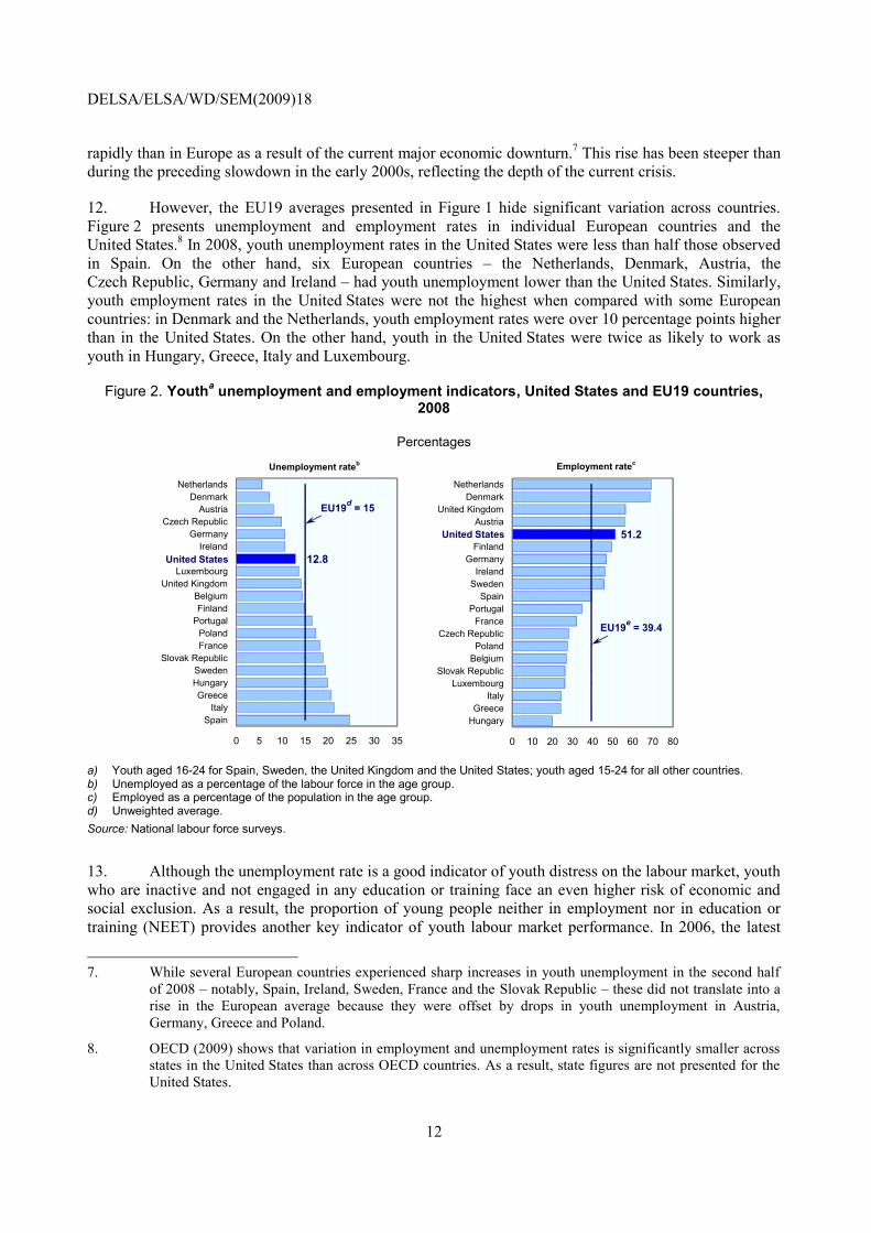
12. However, the EU19 averages presented in Figure 1 hide significant variation across countries.
Figure 2 presents unemployment and employment rates in individual European countries and the
United States.8 In 2008, youth unemployment rates in the United States were less than half those observed
in Spain. On the other hand, six European countries – the Netherlands, Denmark, Austria, the
Czech Republic, Germany and Ireland – had youth unemployment lower than the United States. Similarly,
youth employment rates in the United States were not the highest when compared with some European
countries: in Denmark and the Netherlands, youth employment rates were over 10 percentage points higher
than in the United States. On the other hand, youth in the United States were twice as likely to work as
youth in Hungary, Greece, Italy and Luxembourg.
Figure 2. Youtha unemployment and employment indicators, United States and EU19 countries,
2008
Percentages
Unemployment rateb Employment rate
c
12.8
0 5 10 15 20 25 30 35
Spain
Italy
Greece
Hungary
Sweden
Slovak Republic
France
Poland
Portugal
Finland
Belgium
United Kingdom
Luxembourg
Ireland
Germany
Czech Republic
Austria
Denmark
Netherlands
United States
EU19d
= 15
51.2
0 10 20 30 40 50 60 70 80
Hungary
Greece
Italy
Luxembourg
Slovak Republic
Belgium
Poland
Czech Republic
France
Portugal
Spain
Sweden
Ireland
Germany
Finland
Austria
United Kingdom
Denmark
Netherlands
United States
EU19e
= 39.4
a) Youth aged 16-24 for Spain, Sweden, the United Kingdom and the United States; youth aged 15-24 for all other countries. b) Unemployed as a percentage of the labour force in the age group. c) Employed as a percentage of the population in the age group. d) Unweighted average.
Source: National labour force surveys.
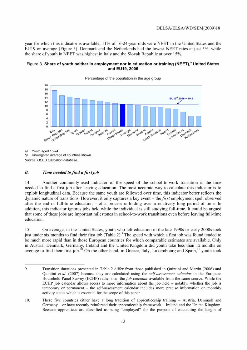
13. Although the unemployment rate is a good indicator of youth distress on the labour market, youth
who are inactive and not engaged in any education or training face an even higher risk of economic and
social exclusion. As a result, the proportion of young people neither in employment nor in education or
training (NEET) provides another key indicator of youth labour market performance. In 2006, the latest
7. While several European countries experienced sharp increases in youth unemployment in the second half
of 2008 – notably, Spain, Ireland, Sweden, France and the Slovak Republic – these did not translate into a
rise in the European average because they were offset by drops in youth unemployment in Austria,
Germany, Greece and Poland.
8. OECD (2009) shows that variation in employment and unemployment rates is significantly smaller across
states in the United States than across OECD countries. As a result, state figures are not presented for the
United States.
DELSA/ELSA/WD/SEM(2009)18
13
year for which this indicator is available, 11% of 16-24-year olds were NEET in the United States and the
EU19 on average (Figure 3). Denmark and the Netherlands had the lowest NEET rates at just 5%, while
the share of youth in NEET was highest in Italy and the Slovak Republic at over 15%.
Figure 3. Share of youth neither in employment nor in education or training (NEET),a United States
and EU19, 2006
Percentage of the population in the age group
0
2
4
6
8
10
12
14
16
18
20
EU19b
2006 = 10.9
a) Youth aged 15-24. b) Unweighted average of countries shown.
Source: OECD Education database.
B. Time needed to find a first job
14. Another commonly-used indicator of the speed of the school-to-work transition is the time
needed to find a first job after leaving education. The most accurate way to calculate this indicator is to
exploit longitudinal data. Because the same youth are followed over time, this indicator better reflects the
dynamic nature of transitions. However, it only captures a key event – the first employment spell observed
after the end of full-time education – of a process unfolding over a relatively long period of time. In
addition, this indicator ignores jobs held while the individual is still studying full-time. It could be argued
that some of these jobs are important milestones in school-to-work transitions even before leaving full-time
education.
15. On average, in the United States, youth who left education in the late 1990s or early 2000s took
just under six months to find their first job (Table 2).9 The speed with which a first job was found tended to
be much more rapid than in those European countries for which comparable estimates are available. Only
in Austria, Denmark, Germany, Ireland and the United Kingdom did youth take less than 12 months on
average to find their first job.10
On the other hand, in Greece, Italy, Luxembourg and Spain,11
youth took
9. Transition durations presented in Table 2 differ from those published in Quintini and Martin (2006) and
Quintini et al. (2007) because they are calculated using the self-assessment calendar in the European
Household Panel Survey (ECHP) rather than the job calendar available from the same source. While the
ECHP job calendar allows access to more information about the job held – notably, whether the job is
temporary or permanent – the self-assessment calendar includes more precise information on monthly
activity status which is essential for the scope of this paper.
10. These five countries either have a long tradition of apprenticeship training – Austria, Denmark and
Germany – or have recently reinforced their apprenticeship framework – Ireland and the United Kingdom.
Because apprentices are classified as being “employed” for the purpose of calculating the length of

DELSA/ELSA/WD/SEM(2009)18
14
about two years on average to find a job after leaving education. However, long average spells of
non-employment after leaving education before finding the first job were often the result of very wide
distributions. For instance, in France, it took 14 months to find a first job on average, but the 50% of youth
who found work the fastest did so within just two months of leaving education while the slowest 10% took
4½ years. It is noteworthy that in the United States as well as in several European countries, at least 50% of
youth already had a job when leaving education.12
Table 2. Months needed to find a first job after leaving school, United States and Europe,a
late 1990s-early 2000s
Mean Median 75th percentile 90th percentile
United States 5.6 0 4.4 18.8
North East 5.3 0 4.1 17.9
North Central 4.1 0 2.3 14.1
South 6.6 0 6.5 22.4
West 5.4 0 3.5 18.5
Europe 16.9 3 23.0 59.0
Austria 5.7 0 12.0 14.6
Belgium 17.5 3 23.0 67.4
Denmark 6.3 0 5.0 17.1
France 14.4 2 21.0 54.0
Germany 5.0 0 3.0 14.0
Greece 24.4 12 38.3 71.0
Ireland 8.3 0 6.0 25.8
Italy 33.1 24 53.0 95.0
Luxembourg 21.6 3 18.8 95.0
Portugal 15.6 3 17.0 61.8
Spain 22.1 12 31.0 73.4
United Kingdom 5.8 0 2.0 12.0
a) Finland is excluded from this table because the presence of missing values did not allow us to derive a reliable estimate for the time needed to find the first job after leaving education.
Source: Secretariat calculations based on the National Longitudinal Surveys of Youth 1997 and the European Community Household Survey (1994-2001).
transitions, this contributes to shorter transitions in countries where apprenticeship schemes are
widespread. The role of apprenticeships is analysed in more detail in Section 5.
11. It is noteworthy that these long transitions obtained using calendar data from a longitudinal survey are
sometimes at odds with those obtained when youth are asked directly about the time it took them to find
their first job. The difference from the two sources is striking in the case of Spain for which the survey data
used in this paper produces transition durations of close to two years while an alternative database –
Juventud en España – suggests estimates of just six months (OECD, 2007). The exact reasons behind this
large difference cannot be identified, but it is possible that youth take short-lived, part-time, informal jobs
into account when asked about the duration of their school-to-work transition while they tend to
under-report these less significant jobs in surveys where they have to give the exact timing and
characteristics of all their activity statuses.
12. Entry jobs that started before/upon finishing education are not necessarily of short duration. In the
United States, one in five youth leaves school holding a job that will last at least another 12 months.
DELSA/ELSA/WD/SEM(2009)18
15
3. Classifying transitions through sequence analysis
16. In a simplified theoretical model of school-to-work transitions, youth leave education, search
for work and find a job that allows them to get a firm foothold into the labour market. In this framework,
the measures presented in Table 2 are a good summary indicator of the length of school-to-work
transitions. However, when longitudinal data are explored, it becomes clear that such a simplified
theoretical framework only provides a partial description of school-to-work transitions as it disregards
the varying dynamics experienced by youth over the period between leaving school and entering stable
employment.13
17. To fully account for the dynamic nature of early labour market participation, this section uses a
technique that is entirely driven by data. Hence, much like other data-driven techniques – e.g. factor
analysis – it allows us to explore a dataset and discover (or confirm) some underlying patterns without any
priors based on economic theory. Three steps are required to conduct the analysis: i) individual sequences
of all the main activity statuses – i.e. individual trajectories – experienced over the five years after leaving
secondary education are constructed; ii) the distance between trajectories is measured; and iii) the most
similar trajectories are grouped together and, if the results look consistent, each group is interpreted as a
distinct school-to-work pathway.
A. Defining individual trajectories
What is a trajectory?
18. For the purpose of quantitative analysis, a trajectory is just a sequence of monthly activity
statuses. Selected statuses must be mutually exclusive to make sure that each sequence unambiguously
describes the young person‟s trajectory upon leaving high school. The set of statuses that can be used in the
sequences depends on the data available, on the group of youth included in the analysis and on the purpose
of the analysis.
What data are used?
19. For selected European countries, monthly activity statuses of school-leavers are extracted from
the European Community Household Panel (ECHP) survey (waves 1994-2001).14
For the United States,
they are taken from the two cohorts of the National Longitudinal Surveys of Youth: the 1997 cohort and
the 1979 cohort. The analysis is limited to youth who have left education at ISCED level three or lower –
i.e. holding at most an upper-secondary qualification – and who are observed in the panel for at least
60 months. Youth are coded as having left education when they are observed in employment, inactivity or
unemployment for the first time. Tertiary leavers are not included to ensure comparability between the
United States and European data. For the United States, the most recent data are based on a cohort of youth
aged 14 or 15 in 1997 and observed until 2005. As a result, hardly any follow-up data are available for
youth leaving tertiary education. In Europe, survey data would allow the inclusion of tertiary leavers but
this would distort comparisons with the United States.
13. The dynamic nature of youth labour market participation was first explored in the early 1980s by Freeman
and Wise (1982) and OECD (1984). Both studies highlighted the blurred distinction between
unemployment and labour force withdrawal for youth and concluded that changes in labour force status
between employment, unemployment and not-in-the-labour force were more frequent among youth than
adults. They also highlighted the existence of a hard-core of disadvantaged youth who bore most of the
brunt of long spells of unemployment or inactivity.
14. The countries are: Austria, Belgium, Denmark, France, Germany, Greece, Ireland, Italy, Luxembourg,
Portugal, Spain, and the United Kingdom.

DELSA/ELSA/WD/SEM(2009)18
16
What assumptions are needed?
20. For the purpose of comparing pathways in the United States and in Europe, only four statuses
are retained – employed, unemployed, inactive but not in education (from here onwards inactive), and in
education15
– and individuals are not allowed to be in more than one status at each point in time. As a
result some assumptions must be made: i) youth working during the school year or during school
holidays are coded as being in education; ii) apprentices are counted as employed; iii) no distinction is
made between temporary and permanent employment; iv) all jobs are treated equally, irrespective of the
number of hours worked; and v) youth complying with compulsory military service regulations are
counted as inactive.16
21. Although unavoidable, some of these assumptions are likely to affect the outcomes of the
analysis. First, the nature of the analysis implies that only one status can be retained for each month while
some individuals may combine two activities – notably, employment and education or job search and
education.17
The choice of a dominant status is not unusual when labour market data are concerned. For
instance, in labour force surveys, one hour of paid work in the reference period suffices to classify
someone as employed even if the individual was unemployed or inactive the rest of the time. In the context
of school-to-work transitions, education is retained as the dominant status. Hence, as mentioned above,
youth working during the school year or during school holidays are coded as being in education. This is a
strong assumption as some of the jobs held during education can have an impact on future career prospects,
hence affect the trajectory of an individual after he/she leaves full-time initial education. Section 6 of this
paper sheds some light on this issue.
22. Second, participation in an apprenticeship is not coded as a separate status because
apprenticeship spells can only be identified in the ECHP and not in the NLSY. Finally, individuals are
coded as employed with no regard to job quality – i.e. temporary jobs are treated the same way as
permanent jobs. Section 5 of this paper explores the role of apprenticeships and temporary work in
transitions from school to work in European countries.
15. While youth are observed starting from the month when they leave school, some return to education later
in the transition period.
16. In the EU19 sample retained for analysis, time spent in military service accounts for about 1.7% of the total
months observed.
17. In practice, this issue only arises for the United States. In fact, while the NLSY contains information about youth
combining work and study, the ECHP self-assessment calendar only reports one status per month – i.e. the status
that the interviewee regards as being his main activity during that month. However, other sources suggest that
youth in EU19 countries less frequently combine work and study than their U.S. counterparts. In the NLSY
sample of school-leavers used in the analysis, 36.7% had worked while in school. The European Labour Force
Survey suggests that only 14.8% of 15-19-year-old students worked in 2006.

DELSA/ELSA/WD/SEM(2009)18
17
B. Measuring the distance between individual trajectories
23. The second step in identifying school-to-work pathways consists in assessing the degree of
similarity between individual trajectories. Several methodologies exist to calculate the “distance” between
vectors of qualitative variables.18
The one used in this paper, Optimal Matching (OM), is an explorative
method of sequence analysis developed by molecular biologists in order to find similar patterns within
DNA.19
Abbot and Forest (1986) were the first to apply OM in a social science context. To the best of our
knowledge, only five studies have applied the technique to sequences of activity statuses in the phase of
transition from school to work20
(Halpin and Chan, 1998; Scherer, 1999; Schoon et al., 2001;
Anyadike-Danes and McVicar, 2003; and Brzinsky-Fay, 2007).
24. Box 1 provides an example of how OM works based on school-to-work individual trajectories. The
OM procedure consists in calculating the distance between each pairwise combination of sequences. The
distance between two sequences is, roughly speaking, the number of steps one must perform in order to make
both sequences equal. In this process, which is named „alignment‟, there are three possible operations
available: an item can be substituted by another item, an item can be inserted into a sequence, or an item can
be deleted from a sequence – the so-called indel (insert and delete) operations. The decision regarding the
quantification of these operations is left to the researcher and may need to be justified by theory. The values
used in the analysis are those used by Brzinsky-Fay (2007): indel costs are set as equal to one, whereas
substitution costs are set at two.21
Because there is more than one solution for the alignment of two
sequences, the OM algorithm always calculates the minimum distance between two sequences.
25. The OM procedure for European countries is carried out on the whole European sample as no
single country has enough observations to be analysed separately. As a result, not all pathways may be
present in all countries included in the sample.
18. Grelet (2002) provides an overview of alternative methodologies.
19. DNA can be translated into amino-acid sequences (proteins) through the use of the so-called genetic code.
Comparing the amino-acid sequences in a particular protein in different species allows one to understand
the evolutionary relationships between organisms. In this context, OM is used to calculate the minimum
number of mutations that must have occurred for the two organisms to diverge (note that evolution usually
takes the most economic course). Scientists can then derive the number of years needed for the mutation to
take place. The greater the difference in amino acid sequences the smaller the evolutionary closeness
between the two organisms. For example, amino-acid sequences of the insulin protein are identical in
humans, rabbits, dogs, pigs and macaques, have one amino-acid difference in rats, mice and hamsters, and
a few differences in elephants, horses, camels, sheep, etc.
20. A similar methodology using a simpler distance measure is employed by Céreq in France to identify
school-to-work pathways among cohorts of school-leavers (Cereq, 2005). Compared with OM, the
methodology used by Céreq tends to overestimate the distance between sequences as similarities between
sequences are less easily detected.
21. Brzinsky-Fay (2007), Schoon et al. (2001) and Anyadike-Danes and McVicar (2003) have experimented with
different variants of substitution and indel costs but results show only very slight differences.

DELSA/ELSA/WD/SEM(2009)18
18
Box 1. Calculating the distance between school-to-work trajectories: an example
Individual trajectories derived from ECHP and NLSY include 60 monthly activity statuses, i.e. they are sequences of 60 cells. As a result, it is impractical to use them as an example. Instead, the following two short sequences of five activity statuses provide enough variation to show how the distance between two sequences is calculated.
Month 1 Month 2 Month 3 Month 4 Month 5
Glenda Inactivity Unemployment Employment Employment Employment
Thomas Unemployment Employment Employment Employment Education
Glenda took a month off travelling after leaving education; she started looking for work upon her return in month two, found a job in month three and remained employed for three months. Thomas started looking for work straight away after leaving education; he found work in month two and remained employed for three months; in month five he decided to return to education to obtain a university degree.
What is the distance between the Glenda’s and Thomas’ trajectories?
The distance between two sequences depends on the number of steps one must perform in order to make both sequences equal. However, even for simple sequences such as those presented here, there may be more than one option to do so. One way of making Glenda’s and Thomas’ sequences equal is to operate the following three substitutions:
Transformation A
Month 1 Month 2 Month 3 Month 4 Month 5
Glenda Inactivity Unemployment Employment Employment Employment
Thomas Unemployment Employment Employment Employment Education
Inactivity Unemployment Employment
However, these substitutions ignore the fact that the two sequences include four components that are identical – i.e. the same activity statuses in the same order. As a result, another way of making the two sequences equal is to delete Education at the end of Thomas’ sequence and insert Inactivity at the beginning of his sequence:
Transformation B
Month 1 Month 2 Month 3 Month 4 Month 5
Glenda Inactivity Unemployment Employment Employment Employment
Thomas Unemployment Employment Employment Employment Education
Inactivity

DELSA/ELSA/WD/SEM(2009)18
19
Box 1. Calculating the distance between school-to-work trajectories: an example (cont.)
Each transformation shown above needs to be translated into a measure of the distance between Glenda’s and Thomas’ sequences based on the number of steps that are required to make the sequences equal. Transformation B involves just two steps: one deletion and one insertion. On the other hand, each of the three substitutions in Transformation A can be seen as involving two steps – one deletion and one insertion – so six steps are performed as a whole. If a value of one is attributed to each deletion and insertion, Transformation B would translate into a distance of two and transformation A into a distance of six. Hence, Optimal Matching would retain two as the distance between the two sequences – i.e. the shortest way to make the two sequences identical.*
How sensitive is the outcome to the values attributed to insert, delete and substitution operations?
The values attributed to insert, delete and substitution operations in order to translate transformations into measures of distance are, to some extent, arbitrary. Counting the number of steps involved in each transformation appears to be the least controversial choice and it results in the following two conventions: first, insert and delete operations are given a value of one; second, a substitution is worth twice as much as an insertion or deletion.
The first convention is fairly neutral: if a value of two rather than one was attributed to each step, assuming the second convention holds (i.e. substitutions are worth two steps), all distances would be scaled up but the outcome of the OM procedure would not change. The second convention is not neutral but, as it stands, it requires no a-priori economic assumptions: a substitution is simply seen as the combination of deleting one activity and inserting a new one so that both sequences have the same activity in the same cell. Other assumptions could be made but would need to be justified in some way. For instance, it could be argued that the timing of an activity is extremely important, so similar patterns experienced at different times (i.e. Thomas’ experiences the pattern Unemployment Employment Employment Employment one month earlier than Glenda) should not be counted as a similarity between two sequences. As a result, a substitution would be quantified as less than twice an insertion/deletion.
*. This illustrates well the advantage of OM over other measures of distance between sequences which do not allow for indel operations. For instance, the Céreq methodology, which only allows for substitution operations, would score the difference between these two sequences as 6.
C. Grouping trajectories into pathways
26. The final step to identify representative school-to-work pathways consists in grouping together
individual sequences that are similar to each other, i.e. that have the smallest distance between themselves.
To do so, the pairwise distances measured as described in Box 1 are used to construct a distance matrix on
which cluster analysis is carried out.
27. The distance matrix is a symmetric matrix where rows (i) and columns (j) represent the
individuals in the sample and each cell aij contains the distance between the sequence of individual i and
that of individual j. The cells on the diagonal of the matrix contain only zeros because they represent the
distance between an individual‟s sequence and itself. Once the matrix is ready, Ward‟s hierarchical
agglomerative algorithm is applied to group individuals into clusters. As all possible groupings of
individuals are explored, the algorithm chooses the ones that minimise the increase in the within-cluster
error sum-of-squares.22
22. Ward‟s rationale is to minimize the loss of information associated with each grouping, defined as the sum
of the squared distances of individuals from the centre of gravity (mean of distances) of the cluster –
i.e. the error sum-of-squares. Like for other hierarchical agglomerative methods, at the start of the process,
each cell in the distance matrix – each pair of individuals ij – represents a cluster and has distance aij
associated to it. These primitive clusters are then progressively merged and, at every round, the distance
between each two clusters is recalculated using the error sum-of-squares criterion and used in a new,
smaller, distance matrix.

DELSA/ELSA/WD/SEM(2009)18
20
28. Because conventional test statistics are not applicable with sequence data and there is no
economic a priori underlying the OM technique, other arguments must be used to define the appropriate
number of clusters, such as the number of observations in each cluster and their graphical representation.
The latter helps to understand what youth in each cluster have in common and whether the cluster is
analytically meaningful.
D. Graphical representation of the clusters
29. There are two ways of representing each cluster graphically. Using data from waves 1994-2001
of the ECHP survey, Panel A of Figure 4 shows, for each month (horizontal axis), the share of youth in
each of the four activity statuses retained in the analysis (vertical axis). This graphical representation is
easy to read but, because it does not follow individuals over time, it cannot be used by itself to determine
the characteristics of a cluster. For instance, while Panel A clearly shows that a significant share of youth is
still unemployed at the end of the observation period, it is unclear whether these are: the same youth who
were unemployed at month one and remained unemployed thereafter; an entirely different group of young
people who became unemployed later over the observation period; or a combination of the two.
30. Panel B of Figure 4 conveys more accurate information in this respect as each line represents an
individual trajectory with a different colour for each activity status – i.e. months are shown on the
horizontal axis and individual trajectories are shown on the vertical axis and should be read from left to
right. The individual trajectories have been sorted by activity status starting from the one at month 0. From
Panel B, it is clear that youth who are unemployed at month 60 are the combination of two groups: a small
share of youth who have been continuously unemployed over the entire observation period and some youth
who were not unemployed upon leaving school but entered unemployment later in their trajectory. Because
the graphical representation given in Panel B is more informative and less misleading than the one in
Panel A, it is retained in what follows. Unfortunately, it is also more difficult to read. For this reason, a
graphical representation of each pathway along the lines of Panel A is presented in the Annex.
Figure 4. Graphical representation of clusters: an example based on selected European countries
Sequences of labour market and activity spells
B. Individual representationA. Cohort representation
0
10
20
30
40
50
60
70
80
90
100
0 10 20 30 40 50 60
Inactive Unemployed Employed In education
0
200
400
600
800
1000
1200
0 20 40 60
Source: Secretariat calculations based on the European Community Household Panel survey, waves 1 to 8 (1994 to 2001).

DELSA/ELSA/WD/SEM(2009)18
21
E. The pathways
31. Cluster analysis reveals the existence of nine groups which can be each interpreted as a distinct
school-to-work pathway.23
Yet, the extent to which each cluster can be seen as a meaningful pathway varies. For a
number of groups – particularly those where individual trajectories are dominated by one or two activity statuses –
identifying what individual trajectories have in common is straightforward. For groups in which individuals
alternate several activity statuses, patterns emerge less clearly and are more subject to interpretation.
32. Figures 5 to 15 plot sequences of activity statuses over a 60-month period for individuals
belonging to each cluster and report the share of time they spent in education, employment,
unemployment, and inactivity. The figures help to identify what the trajectories of youth in each cluster
have in common and match pathways across areas (Europe and the United States) and time (the 1997 and
1979 cohorts in the United States). Table 3 contains additional useful statistics to understand differences
between the pathways and Box 2 provides guidance on how to read the Figures. In order to see the clusters
more clearly, colours are essential, hence the figures should be printed in colour or looked at on the screen.
Box 2. Interpreting Figures 5 to 15
Entire individual trajectories are plotted and must be read from left to right
In each Figure, entire individual trajectories are plotted horizontally: i.e. each line, from left to right, represents the 60 monthly activity statuses experienced by one individual in the cluster. The number on the vertical axis corresponds to the number of individuals in the cluster and months are reported on the horizontal axis. Four different colours are used for the four activity statuses youth can experience.
Statistics on the share of the 60 months spent in each activity status
Each Figure also reports the average share of time that youth belonging to that cluster spent in each of the four activity statuses: education, employment, unemployment, and inactivity. This is shown under each plot.
Dominant colours should be identified as well as their order, from left to right
In the first cluster, the so-called “Express” pathway, plotted in Figure 5, the dominant colour is lavender – the colour associated to employment. This suggests that most youth in this graph found work fairly quickly after leaving education and remained in employment thereafter – either in the same job or through a number of job-to-job moves. Indeed, the share of time spent in employment by youth in this cluster (reported under each plot) exceeds 90% across areas (United States and Europe) and cohorts (1997 and 1979 cohorts in the United States).
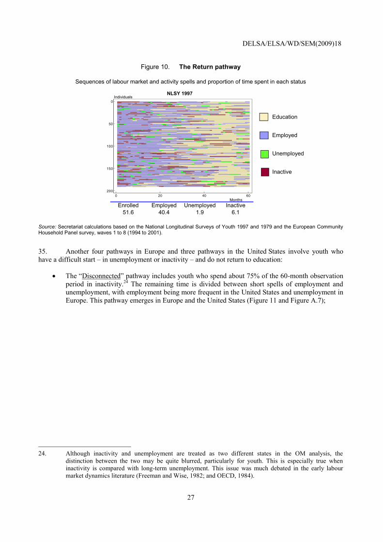
Figure 10 illustrates the case where both dominant colours and their order are needed to spot a meaningful pattern for youth in the cluster. Two colours are dominant: lavender (employment) and light khaki (education). Lavender is concentrated in the first half of the plot while light khaki dominates the second half. As a result, one can conclude the youth in this pathway, the so-called “Return” pathway, have in common the fact that they worked for 2-3 years before returning to education.
The visual interpretation of the sequences and the statistics presented under the plots are complementary
Although, from the plots in Figure 5, one may get the impression that individual trajectories include more inactivity at labour market entry in the United States – particularly in the 1979 cohort – than in Europe, the share of time spent in inactivity is very similar across areas and cohorts. In fact, because sample size (shown on the vertical axis) varies significantly across the three databases, this influences the visual appearance of the plots which may give false impressions on the share of time spent in education, employment, unemployment and inactivity in each pathway.
The inverse is also true and the time shares cannot be used alone to define a pathway as the plots add key information on the sequence of events. For instance, for the United States 1997 cohort, trajectories plotted in Figures 13 and 14 present a similar share of inactivity: 35% and 41%, respectively. However, the plots show that, while in Figure 13 inactivity is concentrated at the end of the individual trajectories, in Figure 14 it is concentrated in the months immediately following school-leaving. Hence, youth in Figures 13 and 14 are classified as belonging to two different pathways, the so-called “Discouraged” and “Recovery” pathways respectively.
23. The presence of more or fewer clusters has been investigated, but the identification of the pathways was
the clearest and most comparable across areas when nine clusters were created.

DELSA/ELSA/WD/SEM(2009)18
22
33. In both Europe and the United States, it is possible to identify two pathways dominated by
employment:
The “Express” pathway including youth who spend over 90% of their time on average in
employment (Figure 5 and Figure A.1);
Figure 5. The Express pathway
Sequences of labour market and activity spells and proportion of time spent in each status
Education
Employed
Unemployed
Inactive
Enrolled Employed Unemployed Inactive
2.73.092.81.5
Enrolled Employed Unemployed Inactive
3.9 91.0 2.2 2.90.6 93.3 3.5 2.6
InactiveEnrolled Employed Unemployed
0
200
400
600
800
0 20 40 60
0
500
1000
1500
2000
0 20 40 60
0
100
200
300
400
0 20 40 60
ECHP 1994 NLSY 1997
NLSY 1979
Months Months
Months
Individuals Individuals
Individuals
Source: Secretariat calculations based on the National Longitudinal Surveys of Youth 1997 and 1979 and the European Community Household Panel survey, waves 1 to 8 (1994 to 2001).
The “In-and-Out” pathway including youth who spend a significant time in employment over the
five years (65-70%), but who also experience multiple spells of unemployment (about 10% of the
time altogether) or inactivity (15-20% of the time) – i.e. they tend to experience more instability
than youth in the “express” pathway (Figure 6 and Figure A.2).

DELSA/ELSA/WD/SEM(2009)18
23
Figure 6. The In-and-Out pathway
Sequences of labour market and activity spells and proportion of time spent in each status
Education
Employed
Unemployed
Inactive
Enrolled Employed Unemployed Inactive
8.39.972.09.9
Enrolled Employed Unemployed Inactive
1.4 71.6 10.6 16.45.2 64.2 11.3 19.3
InactiveEnrolled Employed Unemployed
0
100
200
300
400
0 20 40 60
0
50
100
0 20 40 60
0
200
400
600
0 20 40 60
ECHP 1994 NLSY 1997
NLSY 1979
Months Months
Months
Individuals Individuals
Individuals
Source: Secretariat calculations based on the National Longitudinal Surveys of Youth 1997 and 1979 and the European Community Household Panel survey, waves 1 to 8 (1994 to 2001).
34. Three pathways in Europe and four pathways in the United States 1997 cohort involve one or
more spells of education during the five-year observation period:
The “Gap-Year” pathway includes youth who spend a short period of time – approximately one
year – either on the labour market or in inactivity, then return to education and stay in education
thereafter, presumably completing tertiary education. Youth in this group spend between 80%
and 90% of the 60 monthly observations in education. This pathway exists in Europe and in the
recent United States cohort (Figure 7 and Figure A.3);

DELSA/ELSA/WD/SEM(2009)18
24
Figure 7. The Gap-Year pathway
Sequences of labour market and activity spells and proportion of time spent in each status
Education Employed Unemployed Inactive
11.1 1.2 5.75.289.6 2.6 2.5 82.0
Enrolled InactiveUnemployedEmployedEnrolled Employed Unemployed Inactive
0
50
100
150
200
0 20 40 60
0
20
40
60
80
100
0 20 40 60Months
NLSY 1997
Individuals
Months
ECHP 1994
Individuals
Source: Secretariat calculations based on the National Longitudinal Surveys of Youth 1997 and 1979 and the European Community Household Panel survey, waves 1 to 8 (1994 to 2001).
The “Slow-Leavers” pathway includes youth who alternate education spells with inactivity and
labour market spells for the first three years after leaving education. After that, they enter the
labour market with various degrees of success. Youth in this pathway spend 85-90% of their time
in either employment or education. This pathway exists in both Europe and the United States
(Figure 8 and Figure A.4);

DELSA/ELSA/WD/SEM(2009)18
25
Figure 8. The Slow-Leavers pathway
Sequences of labour market and activity spells and proportion of time spent in each status
Education
Employed
Unemployed
Inactive
Enrolled Employed Unemployed Inactive
6.84.419.968.9
Enrolled Employed Unemployed Inactive
50.9 27.3 5.5 16.362.6 23.5 7.9 6.0
InactiveEnrolled Employed Unemployed
0
50
100
150
0 20 40 60
ECHP 1994
0
50
100
150
0 20 40 60
NLSY 1997
0
100
200
300
400
0 20 40 60
NLSY 1979
Months Months
Months
Individuals Individuals
Individuals
Source: Secretariat calculations based on the National Longitudinal Surveys of Youth 1997 and 1979 and the European Community Household Panel survey, waves 1 to 8 (1994 to 2001).
The “Link” pathway includes youth who work for a short period – approximately a year – then
return to education for a short spell before entering work and staying in work thereafter. Youth in
this pathway spend about 25% of their time in education and 50-60% of their time in
employment, mostly after the education spell. This pathway emerges in both Europe and the
United States (Figure 9 and Figure A.5);

DELSA/ELSA/WD/SEM(2009)18
26
Figure 9. The Link pathway
Sequences of labour market and activity spells and proportion of time spent in each status
Education
Employed
Unemployed
Inactive
Employed Unemployed Inactive
29.5 55.9 4.8 9.8
InactiveEnrolled Employed Unemployed Enrolled
34.4 50.8 6.1 8.7
30.4 60.5 6.0 3.1
Enrolled Employed Unemployed Inactive
0
100
200
300
400
0 20 40 60
NLSY 1997
0
50
100
150
200
0 20 40 60
ECHP 1994
NLSY 1979
0
20
40
60
80
100
0 20 40 60Months Months
Months
Individuals Individuals
Individuals
Source: Secretariat calculations based on the National Longitudinal Surveys of Youth 1997 and 1979 and the European Community Household Panel survey, waves 1 to 8 (1994 to 2001).
The “Return” pathway includes youth who successfully enter employment and towards the end of
the observation period decide to return to education. Youth in this pathway spend 40% of their
time in employment and 50% of the time in education after the employment spell. This pathway
only emerges in the United States 1997 cohort (Figure 10 and Figure A.6);
DELSA/ELSA/WD/SEM(2009)18
27
Figure 10. The Return pathway
Sequences of labour market and activity spells and proportion of time spent in each status
Education
Employed
Unemployed
Inactive
Enrolled
51.6
Employed Unemployed Inactive
40.4 1.9 6.1
NLSY 1997
0
50
100
150
200
0 20 40 60
Months
Individuals
Source: Secretariat calculations based on the National Longitudinal Surveys of Youth 1997 and 1979 and the European Community Household Panel survey, waves 1 to 8 (1994 to 2001).
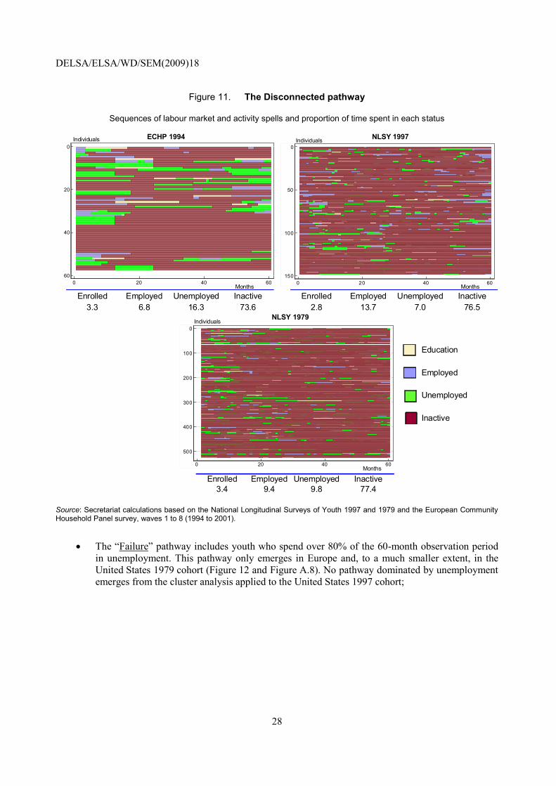
35. Another four pathways in Europe and three pathways in the United States involve youth who
have a difficult start – in unemployment or inactivity – and do not return to education:
The “Disconnected” pathway includes youth who spend about 75% of the 60-month observation
period in inactivity.24
The remaining time is divided between short spells of employment and
unemployment, with employment being more frequent in the United States and unemployment in
Europe. This pathway emerges in Europe and the United States (Figure 11 and Figure A.7);
24. Although inactivity and unemployment are treated as two different states in the OM analysis, the
distinction between the two may be quite blurred, particularly for youth. This is especially true when
inactivity is compared with long-term unemployment. This issue was much debated in the early labour
market dynamics literature (Freeman and Wise, 1982; and OECD, 1984).
DELSA/ELSA/WD/SEM(2009)18
28
Figure 11. The Disconnected pathway
Sequences of labour market and activity spells and proportion of time spent in each status
Education
Employed
Unemployed
Inactive
Employed Unemployed Inactive
2.8 13.7 7.0 76.5
InactiveEnrolled Employed Unemployed Enrolled
3.4 9.4 9.8 77.4
3.3 6.8 16.3 73.6
Enrolled Employed Unemployed Inactive
0
20
40
60
0 20 40 60
0
100
200
300
400
500
0 20 40 60
0
50
100
150
0 20 40 60
NLSY 1997ECHP 1994
NLSY 1979
Months Months
Months
IndividualsIndividuals
Individuals
Source: Secretariat calculations based on the National Longitudinal Surveys of Youth 1997 and 1979 and the European Community Household Panel survey, waves 1 to 8 (1994 to 2001).
The “Failure” pathway includes youth who spend over 80% of the 60-month observation period
in unemployment. This pathway only emerges in Europe and, to a much smaller extent, in the
United States 1979 cohort (Figure 12 and Figure A.8). No pathway dominated by unemployment
emerges from the cluster analysis applied to the United States 1997 cohort;

DELSA/ELSA/WD/SEM(2009)18
29
Figure 12. The Failure pathway
Sequences of labour market and activity spells and proportion of time spent in each status
Education Employed Unemployed Inactive
Enrolled InactiveUnemployedEmployedEnrolled Employed Unemployed Inactive
43.1 42.4 12.510.63.4 81.2 4.8 2.0
0
100
200
300
400
0 20 40 60
0
50
100
150
0 20 40 60Months
NLSY 1979
Individuals
Months
ECHP 1994
Individuals
Source: Secretariat calculations based on the National Longitudinal Surveys of Youth 1997 and 1979 and the European Community Household Panel survey, waves 1 to 8 (1994 to 2001).
The “Discouraged” pathway includes youth who start off by spending a significant time in
unemployment – notably, in Europe – or alternating employment and unemployment – in the
United States – and ultimately leave the labour market to become inactive. This pathway takes
slightly different forms in the recent United States cohort and Europe, but can be found in both
(Figure 13 and Figure A.9);
Figure 13. The Discouraged pathway
Sequences of labour market and activity spells and proportion of time spent in each status
Education Employed Unemployed Inactive
Enrolled InactiveUnemployedEmployedEnrolled Employed Unemployed Inactive
34.5 26.8 35.122.113.7 49.6 14.6 3.6
0
20
40
60
80
0 20 40 60
0
50
100
150
200
0 20 40 60Months
NLSY 1997
Individuals
Months
ECHP 1994
Individuals
Source: Secretariat calculations based on the National Longitudinal Surveys of Youth 1997 and 1979 and the European Community Household Panel survey, waves 1 to 8 (1994 to 2001).
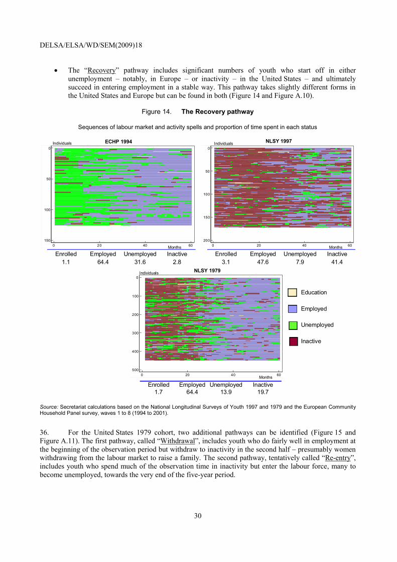
DELSA/ELSA/WD/SEM(2009)18
30
The “Recovery” pathway includes significant numbers of youth who start off in either
unemployment – notably, in Europe – or inactivity – in the United States – and ultimately
succeed in entering employment in a stable way. This pathway takes slightly different forms in
the United States and Europe but can be found in both (Figure 14 and Figure A.10).
Figure 14. The Recovery pathway
Sequences of labour market and activity spells and proportion of time spent in each status
Education
Employed
Unemployed
Inactive
1.7 64.4 13.9 19.7
1.1 64.4 31.6 2.8
Enrolled Employed Unemployed Inactive
InactiveEnrolled Employed Unemployed Enrolled Employed Unemployed Inactive
3.1 47.6 7.9 41.4
0
100
200
300
400
500
0 20 40 60
0
50
100
150
200
0 20 40 60
0
50
100
150
0 20 40 60
NLSY 1997ECHP 1994
NLSY 1979
Months Months
Months
Individuals
Individuals Individuals
Source: Secretariat calculations based on the National Longitudinal Surveys of Youth 1997 and 1979 and the European Community Household Panel survey, waves 1 to 8 (1994 to 2001).
36. For the United States 1979 cohort, two additional pathways can be identified (Figure 15 and
Figure A.11). The first pathway, called “Withdrawal”, includes youth who do fairly well in employment at
the beginning of the observation period but withdraw to inactivity in the second half – presumably women
withdrawing from the labour market to raise a family. The second pathway, tentatively called “Re-entry”,
includes youth who spend much of the observation time in inactivity but enter the labour force, many to
become unemployed, towards the very end of the five-year period.

DELSA/ELSA/WD/SEM(2009)18
31
Figure 15. The Withdrawal and Re-entry pathways
Sequences of labour market and activity spells and proportion of time spent in each status
Education Employed Unemployed Inactive
25.4 18.4 48.246.01.1 9.7 43.2 7.9
Enrolled InactiveUnemployedEmployedEnrolled Employed Unemployed Inactive
0
50
100
150
200
0 20 40 60
0
100
200
300
400
500
0 20 40 60Months
NLSY 1979, Re-entry
Individuals
Months
NLSY 1979, Withdrawal
Individuals
Source: Secretariat calculations based on the National Longitudinal Surveys of Youth 1997 and 1979 and the European Community Household Panel survey, waves 1 to 8 (1994 to 2001).
37. Although most pathways identified for the United States can be matched with similar ones in
Europe, some differences emerge. First, pathways in the United States are characterised by significantly
less time spent in unemployment than in European countries although, to some extent, unemployment was
more of an issue in the United States 1979 cohort (Table 3).
38. Second, all pathways are characterised by more dynamism in the United States than in Europe. In
the “Express” pathway, this translates into more employment spells of shorter duration than in Europe. On
the other hand, in the “Disconnected” pathway, youth in the United States go through more and
significantly shorter spells of inactivity separated by short employment spells while European youth spend
over 34 months in a single inactivity spell on average. Overall, spells of inactivity and unemployment are,
across all pathways, significantly longer in Europe than in the United States.

DELSA/ELSA/WD/SEM(2009)18
32
Table 3. Characteristics of transition sequences, United States (1997-2004 and 1979-1986) and Europea (1994-2001)
Number of spells and average spell duration (in months) in each status and on average
Mean
episodes
Mean
length
Mean
episodes
Mean
length
Mean
episodes
Mean
length
Mean
episodes
Mean
length
United States 1997
Express 0.3 7.1 2.2 24.7 0.7 2.0 0.8 2.1
In-and-Out 0.2 4.0 3.4 12.5 2.1 3.1 2.6 3.8
Gap-Year 1.3 39.0 1.5 4.6 0.3 2.6 0.9 3.8
Slow-Leavers 1.5 20.1 2.5 6.4 1.1 2.9 2.1 4.6
Link 1.4 12.5 3.1 10.8 1.1 2.7 1.8 3.2
Return 1.6 19.0 2.5 9.9 0.6 1.8 1.1 3.2
Disconnected 0.3 6.3 1.9 4.4 1.5 2.7 3.5 12.9
Discouraged 0.3 6.7 3.2 6.4 2.8 5.6 3.5 6.0
Recovery 0.3 7.0 3.2 8.9 1.8 2.6 3.6 6.9
United States 1979
Express 1.2 1.6 2.1 26.1 0.8 2.3 0.8 2.1
In-and-Out 1.7 3.9 3.3 12.7 1.7 3.4 1.6 3.0
Slow-Leavers 2.7 15.4 2.1 5.6 0.9 2.9 1.4 2.9
Link 2.6 8.3 3.1 9.6 1.2 2.9 1.6 3.2
Disconnected 1.3 2.3 1.6 3.5 1.9 3.1 3.3 13.7
Failure 1.2 1.7 3.9 6.6 4.0 6.3 2.4 3.0
Recovery 1.2 1.6 3.1 12.1 2.3 3.6 2.8 4.2
Withdrawal 1.2 1.4 3.1 8.9 1.8 3.2 3.2 7.9
Re-Entry 1.5 3.8 2.6 5.8 2.6 4.2 4.0 7.0
Europe 1994
Express 0.1 3.8 1.6 34.1 0.6 3.4 0.3 5.3
In-and-Out 0.3 9.2 2.4 16.1 1.4 4.8 1.1 10.5
Gap-Year 1.5 36.7 1.0 3.1 0.3 5.1 0.5 2.8
Slow-Leavers 2.3 16.2 2.6 5.4 0.7 6.4 0.6 6.0
Link 1.8 10.4 3.0 12.0 0.9 4.1 0.5 4.0
Disconnected 0.2 9.4 0.6 7.3 0.9 10.9 1.3 33.6
Failure 0.2 9.6 1.0 6.2 2.0 24.6 0.3 8.5
Discouraged 0.8 10.9 1.5 8.5 2.1 14.2 0.9 10.1
Recovery 0.2 4.4 2.3 17.1 2.1 8.9 0.3 4.9
Enrolled Employment Unemployment Inactivity
a) Europe includes the following countries: Austria, Belgium, Denmark, Finland, France, Germany, Greece, Ireland, Italy, Luxembourg, Spain, Portugal and the United Kingdom; United States 1997 refers to the 1997 cohort in the United States; United States 1979 refers to the 1979 cohort in the United States.
Source: Secretariat calculations based on the National Longitudinal Surveys of Youth 1997 and 1979 and the European Community Household Panel survey, waves 1 to 8 (1994 to 2001).
F. Pathways and standard measures of school-to-work transitions compared
39. Table 4 shows that the average time needed to find a first job and the average experience of
NEET vary significantly by pathway. While school-leavers in the United States take on average six months
to find a first job, this transition length varies between about 2.5 months on average for youth in the
“Express” pathway to almost 2.5 years for youth in the “Disconnected” pathway. The average number of
NEET spells and the average time spent in NEET over the 60 months after leaving school also vary
significantly. Youth in the “Express” pathway experience 1.5 spells of NEET for a total length of just three
months, possibly just transitory spells between jobs. At the other extreme, youth in the “Disconnected”
pathway experience as many as five NEET spells for a total duration of 50 months. Similar variation is
observed across European countries. Compared with the United States, youth in the “Express” pathway

DELSA/ELSA/WD/SEM(2009)18
33
take less time to find work – just two weeks on average – but youth in most other pathways take
significantly longer to find their first job than their counterparts in the United States.
40. Tables 3 and 4 underline how the pathways identified by applying OM to monthly activity
sequences incorporate much more information than standard measures of school-to-work transitions such
as the time needed to find a first job. They also summarise how youth attain their first job and whether it
represents an entry port to stable employment or just a short break within a transition dominated by NEET
spells. Indeed, while some pathways differ only marginally in terms of the time needed to find work –
notably the “Express” and “In-and-Out” pathways in the United States – they include very different
experiences of NEET. Also, in the United States, even youth who are the farthest away from the labour
market find work at some point although this does not stop them from spending most of their time over the
observation period in inactivity. This is the case for youth belonging to the “Disconnected” pathway in the
United States who do find work on average within 2.5 years of leaving education but spend 50 months out
of 60 in either unemployment or inactivity.
Table 4. Time needed to find a first job and NEET experience, by pathway, United States and Europe
Months and spell numbers
Time needed to
find first joba
NEET spells in
60 monthsNEET months
Time needed to
find first joba
NEET spells in
60 monthsNEET months
Express 2.7 1.5 3.1 0.5 0.9 3.6
In-and-Out 3.6 4.7 16.2 5.8 2.5 18.3
Gap-Year 3.3 1.2 4.1 10.3 0.8 3.1
Slow-Leavers 5.2 3.2 13.0 11.8 1.3 8.3
Link 4.8 2.9 8.7 1.4 1.4 5.5
Return 4.5 1.8 4.8 - - -
Disconnected 29.0 5.1 49.9 62.7 2.2 53.9
Failure - - - 53.8 2.3 51.3
Discouraged 8.7 6.4 37.0 26.3 2.9 38.2
Recovery 9.6 5.4 29.5 11.1 2.5 20.6
United States 1997 ECHP 1994
- Not applicable.
a) The time needed to find a first job is calculated using the entire follow-up period available (8 years) rather than just the 60 months used for the OM analysis to limit the number of youth for which a value is imputed. This explains why, for example, disconnected youth in Europe appear to take longer than 60 months on average to find their first job.
Source: Secretariat calculations based on the National Longitudinal Surveys of Youth 1997.
4. The size of the pathways in the United States and Europe
41. Figure 16 shows the share of youth in each of the pathways identified in the United States
1979 and 1997 cohorts and in Europe on average. The “Express” pathway includes approximately a third
of school-leavers in both the United States and Europe. If the share of “In-and-Out” youth – where
employment prevails although in a less stable manner than in the “Express” pathway – is added, about 48%
of school-leavers in the United States are mostly employed in their first five years on the labour market
compared with 40% in Europe.

DELSA/ELSA/WD/SEM(2009)18
34
42. The pathways that involve some attachment to education – “Gap-Year”, “Link”, “Return” and
“Slow-Leavers” – count about 31% of youth in the United States and 28% in Europe. While the overall
share is similar, the extent and nature of school attachment to education differs between the United States
and Europe. In Europe, a large share of school-leavers alternates spells of education with inactivity and
labour market spells – the 13% of “Slow-Leavers” – over the first two-thirds of the observation period. On
the other hand, in the United States, only 6% of youth belong to the “Slow-Leavers” pathway while about
8% successfully enter employment after leaving school but “Return” to education later on.
43. Europe has a larger share of youth failing to recover after a difficult start – “Failure”,
“Disconnected” and “Discouraged”– than the 1997 United States cohort. Youth who are trapped in
inactivity for the five years after leaving school are 5% in Europe and 6% in the United States. However,
adding youth who fail to exit unemployment permanently over the five-year period or exit to inactivity
brings the European total to 23% compared with 14% in the United States, mostly due to the fact that
unemployment traps – the “Failure” pathway – do not emerge from the OM analysis on the 1997
United States cohort. On the other hand, the share of European school-leavers recovering from initial
unemployment to enter a stable employment path is – at 10% – larger than the 7% who recovers from
initial inactivity in the United States.
Figure 16. Distribution of youth across transition pathways, Europe and the United States
Percentage of school-leavers in each pathway
0 5 10 15 20 25 30 35 40
Express
In-and-Out
Gap-Year
Slow-Leavers
Link
Return
Disconnected
Failure
Discouraged
RecoveryUnited States 1997
0 5 10 15 20 25 30 35 40
Express
In-and-Out
Gap-Year
Slow-Leavers
Link
Return
Disconnected
Failure
Discouraged
Recovery
Withdrawal
Re-EntryUnited States 1979
0 5 10 15 20 25 30 35 40
Express
In-and-Out
Gap-Year
Slow-Leavers
Link
Return
Disconnected
Failure
Discouraged
RecoveryEurope 1994
Source: Secretariat calculations based on the National Longitudinal Surveys of Youth 1997 and European Community Household Panel survey, waves 1 to 8 (1994 to 2001).
44. Figure 17 presents selected pathways for a number of European countries.25
Close to 80% of
school-leavers in Germany belong to the “express” pathway while a total of only 4.5% take one of the
25. The choice of countries is dictated by sample size.

DELSA/ELSA/WD/SEM(2009)18
35
three negative pathways (“Disconnected”, “Failure” and “Discouraged”).26
At the other end of the
spectrum, in Italy and Spain, very few youth move straight to stable employment and more than a third are
either trapped in unemployment, inactivity or both. The United Kingdom is unusual in that over 55% of
school-leavers enter employment smoothly but a relatively large share – 14% – enters the negative
pathways. Finally, Spain and Portugal have the largest share of school-leavers in the “Recovery” pathway
– i.e. over 15% of them experience prolonged unemployment but ultimately settle into work. It is
noteworthy that differences across the four large United States regions are much less marked (Table 5).
Figure 17. Distribution of youth across key transition pathways, selected European countries, 1994-2001
Percentage of school-leavers in each selected pathway
0
10
20
30
40
50
60
0
10
20
30
40
50
60Ireland
0
10
20
30
40
50
60
0
10
20
30
40
50
60
0
10
20
30
40
50
60
0
10
20
30
40
50
60
Italy Spain
Portugal United KingdomGermany77.4
Source: Secretariat calculations based on the European Community Household Panel survey, waves 1 to 8 (1994 to 2001).
26. This is likely to be due to the treatment of apprenticeships as employment spells in the individual
trajectories. In fact, most German school-leavers enter such a structured pathway. Section 5 of this paper
sheds some light on this issue.

DELSA/ELSA/WD/SEM(2009)18
36
Table 5. Distribution of youth across transition pathways, United States regions, 1997-2005
Percentages
North Central Northeast South West
Express 35.3 30.7 30.7 34.7
Disconnected 4.1 5.9 7.8 3.5
Discouraged 7.7 8.7 9.3 6.6
Recovery 5.1 5.6 8.3 7.2
Source: Secretariat calculations based on the National Longitudinal Surveys of Youth 1997.
5. Understanding variation across Europe
45. The pathways analysis reveals significant variation across European countries, as Figure 17
shows. Not only do countries differ by the distribution of youth in each pathway but it is also possible that,
if examined separately, different pathways would emerge. Indeed, in some European countries,
apprenticeships are a key component of school-to-work transitions. In others, temporary contracts have
expanded significantly over the past few years and have become an almost obligatory entry point for the
vast majority of youth after leaving education. While countries cannot be analysed individually, they can
be grouped together based on the importance of the apprenticeship route and on the incidence of temporary
contracts to identify school-to-work pathways where these two activity statuses play a key role.
46. The group of apprenticeship countries includes: three countries with a long tradition of
apprenticeship training, Austria, Denmark and Germany; and two countries where the apprenticeship
model has been recently reinforced, Ireland and the United Kingdom. In Germany, about 80% of youth in
the ECHP sample entered an apprenticeship lasting at least six months within a year of leaving high
school. One in two youth did so in Austria, one in five in Denmark and one in ten in Ireland and the
United Kingdom. Only in Denmark does the share of youth on involuntary temporary work one year after
school leaving exceed 10%.
47. The group of temporary-work countries includes: Belgium, France, Greece, Italy, Portugal and
Spain. These countries share a high incidence of involuntary temporary work27
at labour market entry,
ranging from over 50% in Spain to 20% in Greece.28
A. The role of apprenticeship training in school-to-work pathways
48. In some European countries included in the analysis, apprenticeships represent an important step
in school-to-work transitions, particularly for high-school graduates deciding not to enrol in tertiary
education.29
Notably, this is the case in the so-called “dual-system” countries where youths spend some
time in education institutions and the remainder at the workplace. Apprenticeships are then part of the
formal educational structure and are usually entered into after completion of compulsory education. They
27. Temporary work is defined as involuntary when the young person has accepted it because he/she could not
find a permanent job.
28. Secretariat calculations based on the European Union Labour Force Survey.
29. Note, however, that some youth may be pursuing tertiary-level apprenticeships.

DELSA/ELSA/WD/SEM(2009)18
37
involve an employment relationship plus formal schooling – normally one and a half to two days per week
– over a period of two to four years.
49. The ECHP survey contains monthly information on apprenticeship status,30
hence it can be
exploited to investigate pathways involving apprenticeships. Eight different pathways emerge when OM
and cluster analysis are applied to the five selected countries: Austria, Denmark, Germany, Ireland and the
United Kingdom. Six of these pathways are similar to those identified for the whole European sample:
“Express”, “In-and-Out”, “Gap-Year”, “Link”, “Disconnected”, and “Failure”. Two new pathways
involving apprenticeships are also found (Figure 18 and Figure A.12). The main difference between the
two appears to be the length of time that the young person spends on an apprenticeship. In the first
pathway, called “Short Apprenticeship”, youth spend on average 25% of their time in an apprenticeship
and then move to work where they spend 70% of their time. In the second pathway, called “Traditional
Apprenticeship”, youth spend close to 60% of their time in an apprenticeship and then move to work where
they spend 30% of their time.31
In both pathways, youth start an apprenticeship immediately after leaving
high school or after a short employment spell and transit to work directly upon completion. Whether
traditional or short apprenticeships dominate in a given country depends largely on the institutional
characteristics of work-based training in the country.
Figure 18. Short and Traditional Apprenticeship pathways
Sequences of labour market and activity spells and proportion of time spent in each status
Education Apprenticeship Employed Unemployed Inactive
3.1 3.369.6
EmployedEnrolled
0.5
Apprenticeship
23.5
Unemployed Employed Unemployed Inactive
30.2 5.1 3.6
Enrolled Apprenticeship
56.74.3
Inactive
0
20
40
60
80
100
120
0 20 40 60
ECHP 1994, Short Apprenticeship
Months
Individuals
Months
Individuals
ECHP 1994, Traditional Apprenticeship
0
10
20
30
0 20 40 60
Source: Secretariat calculations based on the European Community Household Panel survey, waves 1 to 8 (1994 to 2001). The analysis includes Austria, Denmark, Germany, Ireland and the United Kingdom.
30. In the ECHP, apprenticeship status is defined as being on: a paid apprenticeship or training under special
schemes related to employment. It is not possible to refine the definition further.
31. Although, in the ECHP, it is not possible to separate “paid apprenticeships” from “paid training under
special schemes related to employment”, the OM analysis suggests the existence of two pathways of
varying duration involving the apprenticeship status: called herewith “Short Apprenticeships” and
“Traditional Apprenticeships”. Because in most countries apprenticeships tend to take at least two years to
complete, it is possible that youth on “Short Apprenticeships” are, in fact, engaged in “paid training under
special schemes related to employment”.

DELSA/ELSA/WD/SEM(2009)18
38
50. “Short Apprenticeships” last on average 12 months while “Traditional Apprenticeships” are more
than twice as long at 29 months (Table 6). Youth in both pathways spend very little time in NEET over the
five-year observation period and find a job within less than a month.
51. In Germany, over 70% of youth leaving high school and not continuing to tertiary education
embark on a “Traditional Apprenticeship” pathway and another 10% take the shorter option (Figure 19).
Hence, for the group of youth concerned, apprenticeships represent the key school-to-work transition
pathway. On the other hand, in Ireland, the apprenticeship routes coexist with a significant share of youth
transiting directly from high school to stable employment – i.e. the “Express” pathway. On average, in the
five countries included, only 7% of youth remain trapped in inactivity or unemployment after leaving high
school – the “Disconnected” and “Failure” pathways together – and almost 60% embark on stable
employment directly or through apprenticeship training. Overall, apprenticeship training appears to play a
key role in those European countries that outperform the United States as far as transitions from school to
work of low/medium-qualified youth are concerned.
Table 6. Characteristics of pathways specific to apprenticeship countriesa
Number of spells, average spell duration and time needed to find a first job (in months)
Mean episodes
Mean length
Mean episodes
Mean length
Mean episodes
Mean length
Mean episodes
Mean length
Mean episodes
Mean length
Short Apprenticeships Traditional Apprenticeships
0.6
4.7
5.2
0.3
6.2
0.3
9.4
1.2
28.8
1.7
10.7
0.7
1.0
Enrolled
Apprenticeship
Employed
0.1
2.3
1.1
12.3
0.1
1.0
3.8
2.2
19.2
0.8
2.5
0.3
6.9
Unemployed
Inactive
Time needed to find
first job
NEET spells
NEET months
a) Austria, Denmark, Germany, Ireland and the United Kingdom.
Source: Secretariat calculations based on European Community Household Panel survey, waves 1 to 8 (1994 to 2001).
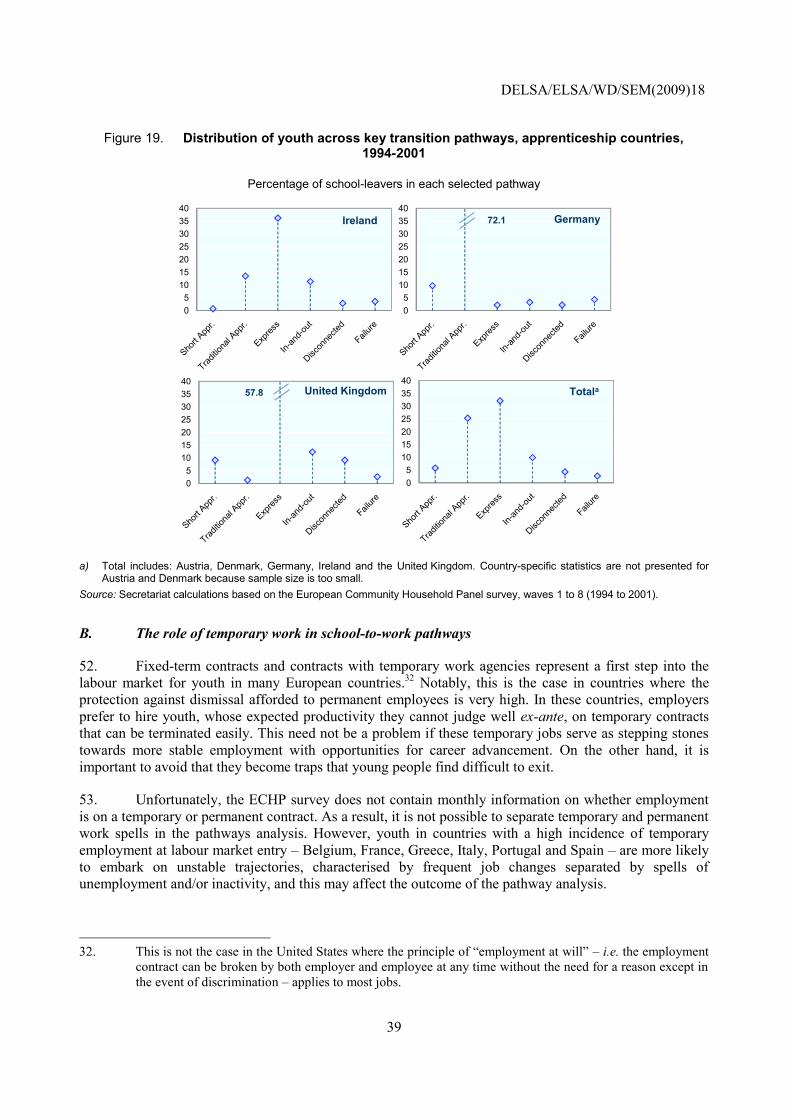
DELSA/ELSA/WD/SEM(2009)18
39
Figure 19. Distribution of youth across key transition pathways, apprenticeship countries, 1994-2001
Percentage of school-leavers in each selected pathway
0
5
10
15
20
25
30
35
40
Ireland
0
5
10
15
20
25
30
35
40
72.1
0
5
10
15
20
25
30
35
40
57.8
0
5
10
15
20
25
30
35
40
Germany
United Kingdom Totala
a) Total includes: Austria, Denmark, Germany, Ireland and the United Kingdom. Country-specific statistics are not presented for Austria and Denmark because sample size is too small.
Source: Secretariat calculations based on the European Community Household Panel survey, waves 1 to 8 (1994 to 2001).
B. The role of temporary work in school-to-work pathways
52. Fixed-term contracts and contracts with temporary work agencies represent a first step into the
labour market for youth in many European countries.32
Notably, this is the case in countries where the
protection against dismissal afforded to permanent employees is very high. In these countries, employers
prefer to hire youth, whose expected productivity they cannot judge well ex-ante, on temporary contracts
that can be terminated easily. This need not be a problem if these temporary jobs serve as stepping stones
towards more stable employment with opportunities for career advancement. On the other hand, it is
important to avoid that they become traps that young people find difficult to exit.
53. Unfortunately, the ECHP survey does not contain monthly information on whether employment
is on a temporary or permanent contract. As a result, it is not possible to separate temporary and permanent
work spells in the pathways analysis. However, youth in countries with a high incidence of temporary
employment at labour market entry – Belgium, France, Greece, Italy, Portugal and Spain – are more likely
to embark on unstable trajectories, characterised by frequent job changes separated by spells of
unemployment and/or inactivity, and this may affect the outcome of the pathway analysis.
32. This is not the case in the United States where the principle of “employment at will” – i.e. the employment
contract can be broken by both employer and employee at any time without the need for a reason except in
the event of discrimination – applies to most jobs.

DELSA/ELSA/WD/SEM(2009)18
40
54. When OM and cluster analysis are applied to the six selected countries, seven of the eight
emerging pathways are similar to those identified for the whole European sample: “Express”,
“In-and-Out”, “Gap-Year”, “Link”, “Disconnected”, “Failure” and “Recovery”. In addition, a pathway
where youth spend 50% of their time in unemployment and 30% in employment – called “Disrupted” – is
identified (Figure 20 and Figure A.13). Youth in the “Disrupted” pathway alternate unemployment, work
and inactivity spells and only during the last year of observation does employment become more dominant.
This pathway may include those youth who find it difficult to enter stable employment and rotate on
several temporary jobs before doing so. The “Recovery” pathway – not found in apprenticeship countries –
may also include some youth on temporary jobs. In fact, youth in this pathway alternate unemployment
and work for one to two years and then appear to move to stable employment. This pathway may include
youth who enter the labour market on temporary contracts which serve as stepping stones and give them
access to career jobs.
Figure 20. Disrupted and Recovery pathways
Sequences of labour market and activity spells and proportion of time spent in each status
Education Employed Unemployed Inactive
Enrolled InactiveUnemployedEmployedEnrolled Employed Unemployed Inactive
60.8 24.2 10.832.56.0 49.9 11.6 4.1
0
20
40
60
80
0 20 40 60
0
20
40
60
80
0 20 40 60Months
ECHP 1994, Recovery
Individuals
Months
ECHP 1994, Disrupted
Individuals
Source: Secretariat calculations based on the European Community Household Panel survey, waves 1 to 8 (1994 to 2001). The analysis includes Belgium, France, Greece, Italy, Portugal and Spain.
55. Youth in the “Recovery” pathway take half the time to find their first job and experience longer
employment spells and shorter unemployment spells than youth in the “Disrupted” pathway (Table 7).
Between 10 and 15% of high-school-leavers in countries with a high incidence of temporary work belong
to the “Recovery” pathway (Figure 21). Much more variation exists across these countries in the share of
youth belonging to the “disrupted” pathway which ranges from 6% in Portugal to 19% in Spain.33
56. Compared with countries where the apprenticeship model is widespread and with the
United States, countries where temporary work represents a key feature of school-to-work transitions also
33. It is noteworthy that in the mid-1990s, when youth included in the analysis left high school, Spain had a
higher incidence of temporary work among youth than the other five countries studied. However, over the
past decade, the incidence of temporary work among youth has risen in Belgium, Italy and Portugal, hence
it is possible that the size of the “disrupted” pathway has increased in these countries.

DELSA/ELSA/WD/SEM(2009)18
41
have a larger share of youth in the “Failure” and “Disconnected” pathways and, with the exception of
Portugal, a smaller share of youth in the “Express” and “In-and-Out” pathways. However, it is important to
keep in mind that, while the labour market duality created by the coexistence of highly protected
permanent jobs and temporary contracts may contribute to the poorer performance of youth in the labour
market, other factors may also be at play.
Table 7. Characteristics of pathways specific to temporary-work countriesa
Number of spells, average spell duration and time needed to find a first job (in months)
Mean episodes
Mean length
Mean episodes
Mean length
Mean episodes
Mean length
Mean episodes
Mean length
NEET spells 3.2
NEET
months36.8
Inactive0.8
9.2
Time needed
to find first 21.2
Employed2.1
9.3
Unemployed2.4
12.2
Disrupted
Enrolled0.4
8.0
2.5
21
10.7
0.8
8.4
1.7
8.5
2.5
11.7
Recovery
0.3
8.5
a) Belgium, France, Greece, Italy, Portugal and Spain.
Source: Secretariat calculations based on European Community Household Panel survey, waves 1 to 8 (1994 to 2001).

DELSA/ELSA/WD/SEM(2009)18
42
Figure 21. Distribution of youth across key transition pathways, temporary-work countries, 1994-2001
Percentage of school-leavers in each selected pathway
0
5
10
15
20
25
30
Italy
0
5
10
15
20
25
30
50.7
0
5
10
15
20
25
30
0
5
10
15
20
25
30
Portugal
Spain Totala
a) Total includes: Belgium, France, Greece, Italy, Portugal and Spain. Country-specific statistics are not presented for Belgium, France and Greece because sample size is too small.
Source: Secretariat calculations based on the European Community Household Panel survey, waves 1 to 8 (1994 to 2001).
6. Socio-demographic determinants of belonging to a transition pathway: the U.S. case
57. Along with labour market and education settings and the state of the cycle, socio-demographic
factors are likely to play a key role in determining individual trajectories. In this respect, understanding
what individual and family characteristics influence the probability of disconnecting from the labour
market and education rather than embarking on a stable employment pathway is important for policy
purposes as it can help to identify at-risk youth at an early stage and to design interventions that prevent
them from disconnecting. Surprisingly, Anyadike-Danes and McVicar (2003) are the only other authors to
have exploited Optimal Matching to address this issue.
58. Individual and family characteristics that affect the probability of belonging to a given pathway
can be identified using a multinomial logit model. The model assumes that individuals experience one of a
number of outcomes – i.e. one of a range of pathways – and that the possible outcomes are unordered,
i.e. they do not happen in any distinct order. The probability that an individual belongs to a particular
pathway can be modelled as a function of their personal characteristics and family situation. This analysis
is only carried out for the United States because only the NLSY database includes sufficiently rich
information on surveyed youth and their families.
59. The nine pathways included in the model are: express, in-and-out, gap year, slow leaver, link,
return, disconnected, discouraged and recovery. Because pathways summarise labour market behaviour

DELSA/ELSA/WD/SEM(2009)18
43
over a period of time, explanatory variables would ideally belong to two sets. The first set includes
unchanging individual characteristics that may impact on the probability of belonging to a given pathway:
race, gender, qualification held when leaving school, mother‟s and father‟s educational level, whether the
young person combined work and study at some point, and the household income when leaving education.
The second set defines events that are likely to affect the way the sequence of monthly observations starts
at school exit and/or the way the sequence progresses: being a mother or a father at school exit or
becoming one by the second observation year; and being married at school exit or getting married by the
second observation year.34
60. Because of the relatively large number of pathways, only the significant coefficients in a number
of comparisons of interest are shown in Table 8. The results are presented as relative risk ratios for each
explanatory variable and alternative. A relative risk ratio shows the relative probability of a young person
with a particular characteristic being in a given pathway compared with the base category. A relative risk
ratio greater than one indicates that the particular characteristic increases the probability that the young
person is in the pathway in question rather than in the baseline pathway. A relative risk ratio smaller than
one indicates that the particular characteristic reduces the probability that a young person is in the pathway
rather than in the baseline pathway. For example, a relative risk ratio of 0.18 for the variable “high-school
graduate at entry” for the “Disconnected” pathway outcome indicates that, compared with a young person
without a qualification, one with a high-school qualification has a much smaller probability of belonging to
the “Disconnected” pathway rather than the “Express” one. The Wald test for combining alternatives
rejects the null hypotheses that any two pathways can be combined given the specification used.
Table 8. Factors affecting the likelihood of belonging to a school-to-work transition pathway, United States
Relative risk ratiosa
Baseline pathway:
In and Out Gap Year Return Recovery Disconnected Slow Leavers Discouraged Return Return Slow Leavers
High school graduate at entry 0.43*** 0.25*** 0.18*** 0.28*** 0.61** 2.54*** 0.28***
Black 1.65** 1.55* 2.04*** 2.61*** 1.68*
Man 0.13*** 0.06*** 3.28** 0.04***
Youth's mother ISCED<3 0.40*** 0.43** 0.37***
Youth's mother ISCED=3 0.55* 0.42**
Married man by year 2 0.52** 0.40** 0.38* 0.10*** 0.35**
Married woman by year 2 0.19*** 0.49* 4.41*** 2.62**
Father by year 2 0.49** 10.51** 0.40** 21.27***
Mother by year 2 2.44*** 5.70*** 7.29*** 2.49** 0.40**
Worked and studied 0.64*** 0.53*** 0.38*** 0.64*
Household income at entry 1.72*** 0.81** 1.22* 0.82** 0.70** 0.71**
Unemployement rate at school
leaving 1.66*** 1.68***
Gap YearExpress In and Out
a) The relative risk ratios are derived from the significant coefficients of a multinomial logit regression of the probability of taking one of the nine pathways identified in this paper. Robust standard errors are calculated and ***, **, * stand for statistically significant at 1%, 5% and 10% levels, respectively. Other variables included but not significant are: Hispanic youth, alcohol and drug consumption, participation in crime, disability.
Source: Secretariat calculations based on the National Longitudinal Surveys of Youth 1997.
61. Table 8 shows that, in the United States, having a high-school qualification when approaching
the labour market reduces the likelihood of belonging to the “In-and-Out”, “Disconnected”, “Recovery”
and “Slow-Leaver” pathways relative to the “Express” pathway, compared with not having a qualification.
It also reduces the likelihood of being a “slow-leaver” relative to returning to attend post-secondary
34. Single parents – predominantly teenage mothers – are too few in the sample to obtain any meaningful
coefficient in the multinomial logit analysis. However, they are concentrated in the disconnected pathway.
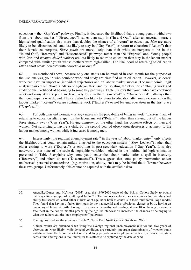
DELSA/ELSA/WD/SEM(2009)18
44
education – the “Gap-Year” pathway. Finally, it decreases the likelihood that a young person withdraws
from the labour market (“Discouraged”) rather than stay in (“In-and-Out”) after an uncertain start; a
high-school qualification also more than doubles the chance of a “return” to education. Men are more
likely to be “disconnected” and less likely to stay in (“Gap-Year”) or return to education (“Return”) than
their female counterparts. Black youth are more likely than their white counterparts to be in the
“In-and-Out”, “Recovery” and “Disconnected” pathways rather than the “Express” one. Young people
with low- and medium-skilled mothers are less likely to return to education than stay in the labour market
compared with similar youth whose mothers were high-skilled. The likelihood of returning to education
after a short break increases with household income.35
62. As mentioned above, because only one status can be retained in each month for the purpose of
the OM analysis, youth who combine work and study are classified as in education. However, students‟
work can have an impact on individual trajectories and on labour market success. The multinomial logit
analysis carried out above sheds some light on this issue by isolating the effect of combining work and
study on the likelihood of belonging to some key pathways. Table 8 shows that youth who have combined
work and study at some point are less likely to be in the “In-and-Out” or “Disconnected” pathways than
their counterparts who did not. They are also less likely to return to education after some experience on the
labour market (“Return”) versus continuing work (“Express”) or not leaving education in the first place
(“Gap-Year”).
63. For both men and women, marriage increases the probability of being in work (“Express”) and of
returning to education after a spell on the labour market (“Return”) rather than staying out of the labour
force straight away (“Gap Year”). Having children, on the other hand, has opposite effects on men and
women. Not surprisingly, having a child by the second year of observation decreases attachment to the
labour market among women while it increases it among men.
64. Interestingly, the regional unemployment rate36
in the year of labour market entry37
only affects
the likelihood that youth remain mildly attached to the education system (“Slow Leavers”) rather than
either exiting to work (“Express”) or enrolling in post-secondary education (“Gap Year”). It is also
noteworthy that none of the socio-demographic variables included in the multinomial logit estimation
presented in Table 8 explains why some youth enter the labour market after a spell in inactivity
(“Recovery”) and others do not (“Disconnected”). This suggests that some policy intervention and/or
unobserved personal characteristics (e.g. motivation, ability, etc.) may be behind the difference between
these two groups. Unfortunately, this cannot be captured with the available data.
35. Anyadike-Danes and McVicar (2003) used the 1999/2000 wave of the British Cohort Study to obtain
pathways for a sample of youth aged 16 to 29. The authors exploited socio-demographic variables and
ability-test scores collected either at birth or at age 10 or both as controls in their multinomial logit model.
They found that having a father from outside the managerial and professional classes at birth, having an
unemployed father at birth, having difficulties with maths and reading at age 10 or having received a
free-meal in the twelve months preceding the age-10 interview all increased the chances of belonging to
what the authors call the “non-employment” pathways.
36. The regions used are the same as in Table 2: North East, North Central, South and West.
37. Similar results are obtained when using the average regional unemployment rate for the five years of
observation. Most likely, while demand conditions are certainly important determinants of whether youth
withdraw from the labour market or spend long periods in unemployment rather than work, variation
across time and regions is too limited for this effect to be captured by the data at hand.

DELSA/ELSA/WD/SEM(2009)18
45
7. Conclusions
65. The main purpose of this paper is to show how a technique used to sequence DNA, Optimal
Matching, can be applied to the analysis of school-to-work transitions in the United States and Europe.
This methodology allows the identification of several pathways taken by youth after leaving education.
Pathways identified using Optimal Matching incorporate significantly more information than traditional
measures of transitions. Rather than focusing on a specific point in time or a single activity such as
employment, inactivity or unemployment, pathways convey information on activities undertaken by youth
over the transition period, their sequence and their persistence. As a result, in addition to showing how
easily youth find their first job, they provide information on how stable their employment history is
thereafter. Similarly, pathways allow judging the extent to which non-employment (unemployment and
inactivity) is just temporary or may constitute a trap.
66. The paper identifies nine representative pathways for both the United States and Europe, eight of
which are present in both areas. Despite strong similarities, pathways in the United States tend to be
characterised by significantly more dynamism than in Europe: youth in employment tend to change jobs
more frequently while inactive or unemployed youth are more likely to experience several short spells
rather than a single long one. Pathways identified for the United States are also characterised by
significantly less unemployment than European ones. The share of school-leavers belonging to pathways
dominated by employment is larger in the United States than in Europe and more youth in the
United States return to education after some labour market experience than in Europe. In addition,
non-employment traps are less frequent in the United States due to the lack of unemployment traps.
67. Because variation in the size of the pathways across Europe is significant, the analysis is repeated
separately for two groups of countries. The first group includes countries where apprenticeships represent a
key step in the transition from school to work of youth leaving education with at most an upper secondary
qualification. In these countries – notably Austria, Denmark, Germany, Ireland and the United Kingdom – a
larger share of youth than in the United States experiences successful school-to-work transitions. Traditional
apprenticeships, lasting at least two years, are the dominant school-to-work transition pathway in Austria,
Denmark and Germany. On the other hand, in Ireland and the United Kingdom, some youth pass through
work-based training to access the labour market while others move directly from school to work.
68. In the second group of European countries – notably, Belgium, France, Italy, Portugal and Spain
– school-to-work transitions are characterised by a high incidence of temporary work. Compared with
apprenticeship countries and with the United States, these countries have a significantly smaller share of
youth belonging to pathways dominated by employment while a larger share of youth appears to enter the
labour market on pathways characterised by significant instability.
69. Finally, several socio-economic characteristics are found to influence the probability that youth
in the United States take a given pathway. For instance, being a school drop-out, a Black youth, a young
man or a young mother in the United States increases the likelihood of being trapped in inactivity.
70. If the analysis could be repeated for more countries, some correlations between the size of the
pathways and structural variables describing the functioning of labour markets and the education system
could be tested. This would allow one to draw some policy conclusions on which institutional settings lead
to the smoothest transitions between school and work, beyond the role of apprenticeships and temporary-
work contracts examined in this paper.
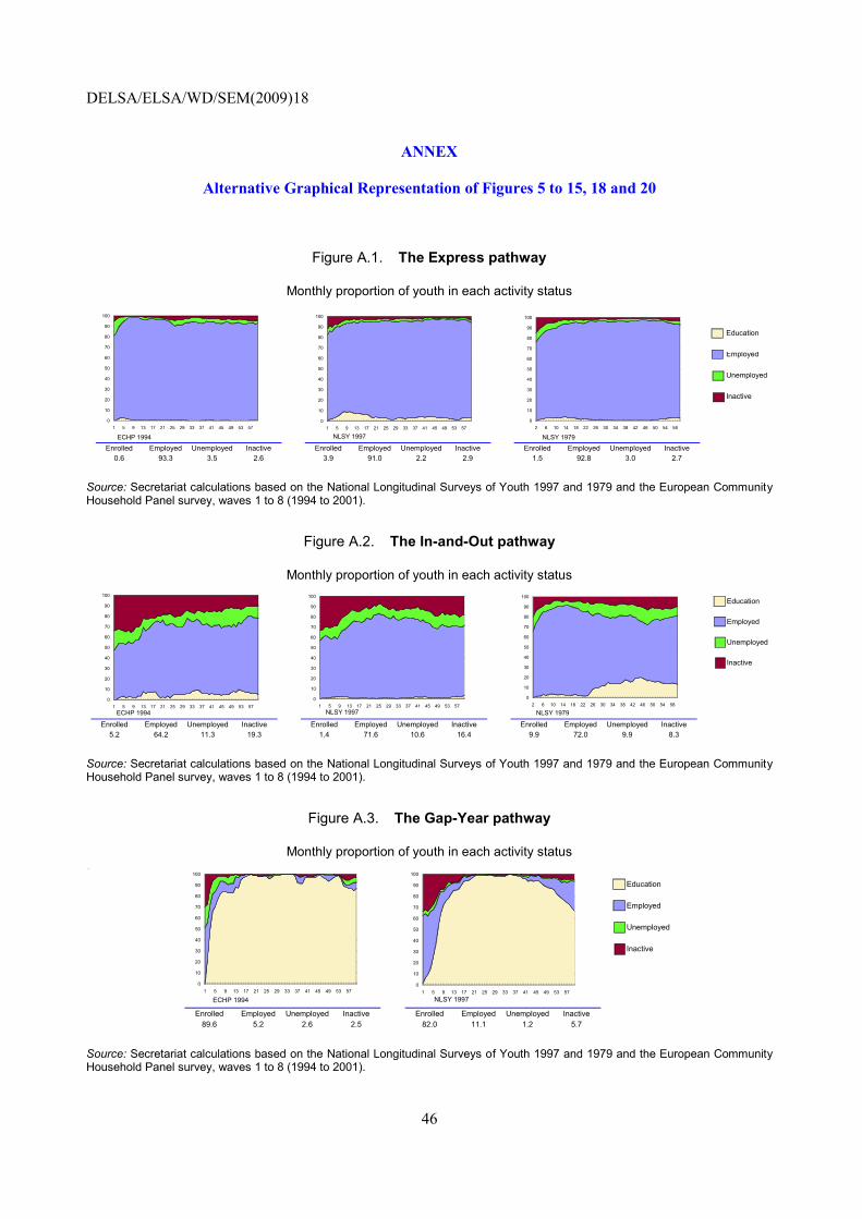
DELSA/ELSA/WD/SEM(2009)18
46
ANNEX
Alternative Graphical Representation of Figures 5 to 15, 18 and 20
Figure A.1. The Express pathway
Monthly proportion of youth in each activity status
Education
Employed
Unemployed
Inactive
Enrolled Employed Unemployed Inactive
2.73.092.81.5
Enrolled Employed Unemployed Inactive
3.9 91.0 2.2 2.90.6 93.3 3.5 2.6
InactiveEnrolled Employed Unemployed
NLSY 1997 NLSY 1979ECHP 1994
0
10
20
30
40
50
60
70
80
90
100
2 6 10 14 18 22 26 30 34 38 42 46 50 54 58
0
10
20
30
40
50
60
70
80
90
100
1 5 9 13 17 21 25 29 33 37 41 45 49 53 57
0
10
20
30
40
50
60
70
80
90
100
1 5 9 13 17 21 25 29 33 37 41 45 49 53 57
Source: Secretariat calculations based on the National Longitudinal Surveys of Youth 1997 and 1979 and the European Community Household Panel survey, waves 1 to 8 (1994 to 2001).
Figure A.2. The In-and-Out pathway
Monthly proportion of youth in each activity status
Education
Employed
Unemployed
Inactive
5.2 64.2 11.3 19.3
InactiveEnrolled Employed Unemployed Enrolled Employed Unemployed Inactive
1.4 71.6 10.6 16.4
Enrolled Employed Unemployed Inactive
8.39.972.09.9
NLSY 1997 NLSY 1979ECHP 1994
0
10
20
30
40
50
60
70
80
90
100
2 6 10 14 18 22 26 30 34 38 42 46 50 54 58
0
10
20
30
40
50
60
70
80
90
100
1 5 9 13 17 21 25 29 33 37 41 45 49 53 57
0
10
20
30
40
50
60
70
80
90
100
1 5 9 13 17 21 25 29 33 37 41 45 49 53 57
Source: Secretariat calculations based on the National Longitudinal Surveys of Youth 1997 and 1979 and the European Community Household Panel survey, waves 1 to 8 (1994 to 2001).
Figure A.3. The Gap-Year pathway
Monthly proportion of youth in each activity status
`
Education
Employed
Unemployed
Inactive
82.0 11.1 1.2 5.789.6 5.2 2.6 2.5
Enrolled Employed Unemployed InactiveInactiveEnrolled Employed Unemployed
ECHP 1994 NLSY 1997
0
10
20
30
40
50
60
70
80
90
100
1 5 9 13 17 21 25 29 33 37 41 45 49 53 57
0
10
20
30
40
50
60
70
80
90
100
1 5 9 13 17 21 25 29 33 37 41 45 49 53 57
Source: Secretariat calculations based on the National Longitudinal Surveys of Youth 1997 and 1979 and the European Community Household Panel survey, waves 1 to 8 (1994 to 2001).
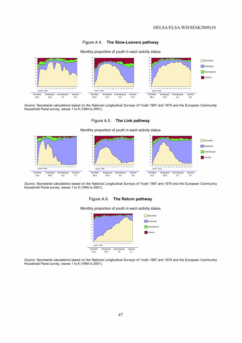
DELSA/ELSA/WD/SEM(2009)18
47
Figure A.4. The Slow-Leavers pathway
Monthly proportion of youth in each activity status
Education
Employed
Unemployed
Inactive
Enrolled Employed Unemployed Inactive
6.84.419.968.9
Enrolled Employed Unemployed Inactive
50.9 27.3 5.5 16.362.6 23.5 7.9 6.0
InactiveEnrolled Employed Unemployed
ECHP 1994 NLSY 1997 NLSY 1979
0
10
20
30
40
50
60
70
80
90
100
1 5 9 13 17 21 25 29 33 37 41 45 49 53 57
0
10
20
30
40
50
60
70
80
90
100
1 5 9 13 17 21 25 29 33 37 41 45 49 53 57
0
10
20
30
40
50
60
70
80
90
100
2 6 10 14 18 22 26 30 34 38 42 46 50 54 58
Source: Secretariat calculations based on the National Longitudinal Surveys of Youth 1997 and 1979 and the European Community Household Panel survey, waves 1 to 8 (1994 to 2001).
Figure A.5. The Link pathway
Monthly proportion of youth in each activity status
Education
Employed
Unemployed
Inactive
Enrolled Employed Unemployed Inactive
8.76.150.834.4
Enrolled Employed Unemployed Inactive
29.5 55.9 4.8 9.830.4 60.5 6.0 3.1
InactiveEnrolled Employed Unemployed
ECHP 1994 NLSY 1997 NLSY 1979
0
10
20
30
40
50
60
70
80
90
100
1 5 9 13 17 21 25 29 33 37 41 45 49 53 57
0
10
20
30
40
50
60
70
80
90
100
1 5 9 13 17 21 25 29 33 37 41 45 49 53 57
0
10
20
30
40
50
60
70
80
90
100
2 6 10 14 18 22 26 30 34 38 42 46 50 54 58
Source: Secretariat calculations based on the National Longitudinal Surveys of Youth 1997 and 1979 and the European Community Household Panel survey, waves 1 to 8 (1994 to 2001).
Figure A.6. The Return pathway
Monthly proportion of youth in each activity status
Education
Employed
Unemployed
Inactive
Enrolled Employed Unemployed Inactive
51.6 40.4 1.9 6.1
NLSY 1997
0
10
20
30
40
50
60
70
80
90
100
1 5 9 13 17 21 25 29 33 37 41 45 49 53 57
Source: Secretariat calculations based on the National Longitudinal Surveys of Youth 1997 and 1979 and the European Community Household Panel survey, waves 1 to 8 (1994 to 2001).
DELSA/ELSA/WD/SEM(2009)18
48
Figure A.7. The Disconnected pathway
Monthly proportion of youth in each activity status
Education
Employed
Unemployed
Inactive
3.3 6.8 16.3 73.6
InactiveEnrolled Employed Unemployed Enrolled Employed Unemployed Inactive
2.8 13.7 7.0 76.5
Enrolled Employed Unemployed Inactive
77.49.89.43.4
ECHP 1994 NLSY 1997 NLSY 1979
0
10
20
30
40
50
60
70
80
90
100
1 5 9 13 17 21 25 29 33 37 41 45 49 53 57
0
10
20
30
40
50
60
70
80
90
100
1 5 9 13 17 21 25 29 33 37 41 45 49 53 57
0
10
20
30
40
50
60
70
80
90
100
2 6 10 14 18 22 26 30 34 38 42 46 50 54 58
Source: Secretariat calculations based on the National Longitudinal Surveys of Youth 1997 and 1979 and the European Community Household Panel survey, waves 1 to 8 (1994 to 2001).
Figure A.8. The Failure pathway
Monthly proportion of youth in each activity status
Education
Employed
Unemployed
Inactive
3.4 10.6 81.2 4.8
InactiveEnrolled Employed Unemployed Enrolled Employed Unemployed Inactive
2.0 43.1 42.4 12.5
ECHP 1994 NLSY 1979
0
10
20
30
40
50
60
70
80
90
100
1 5 9 13 17 21 25 29 33 37 41 45 49 53 57
0
10
20
30
40
50
60
70
80
90
100
2 6 10 14 18 22 26 30 34 38 42 46 50 54 58
Source: Secretariat calculations based on the National Longitudinal Surveys of Youth 1997 and 1979 and the European Community Household Panel survey, waves 1 to 8 (1994 to 2001).
Figure A.9. The Discouraged pathway
Monthly proportion of youth in each activity status
Education
Employed
Unemployed
Inactive
13.7 22.1 49.6 14.6
InactiveEnrolled Employed Unemployed Enrolled Employed Unemployed Inactive
3.6 34.5 26.8 35.1
ECHP 1994 NLSY 1997
0
10
20
30
40
50
60
70
80
90
100
1 5 9 13 17 21 25 29 33 37 41 45 49 53 57
0
10
20
30
40
50
60
70
80
90
100
1 5 9 13 17 21 25 29 33 37 41 45 49 53 57
Source: Secretariat calculations based on the National Longitudinal Surveys of Youth 1997 and 1979 and the European Community Household Panel survey, waves 1 to 8 (1994 to 2001).
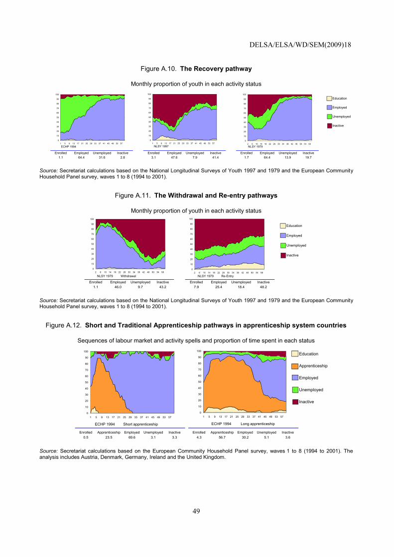
DELSA/ELSA/WD/SEM(2009)18
49
Figure A.10. The Recovery pathway
Monthly proportion of youth in each activity status
Education
Employed
Unemployed
Inactive
Enrolled Employed Unemployed Inactive
19.713.964.41.7
Enrolled Employed Unemployed Inactive
3.1 47.6 7.9 41.41.1 64.4 31.6 2.8
InactiveEnrolled Employed Unemployed
ECHP 1994 NLSY 1997 NLSY 1979
0
10
20
30
40
50
60
70
80
90
100
1 5 9 13 17 21 25 29 33 37 41 45 49 53 57
0
10
20
30
40
50
60
70
80
90
100
1 5 9 13 17 21 25 29 33 37 41 45 49 53 57
0
10
20
30
40
50
60
70
80
90
100
2 6 10 14 18 22 26 30 34 38 42 46 50 54 58
Source: Secretariat calculations based on the National Longitudinal Surveys of Youth 1997 and 1979 and the European Community Household Panel survey, waves 1 to 8 (1994 to 2001).
Figure A.11. The Withdrawal and Re-entry pathways
Monthly proportion of youth in each activity status
Education
Employed
Unemployed
Inactive
Enrolled Employed Unemployed Inactive
7.9 25.4 18.4 48.21.1 46.0 9.7 43.2
InactiveEnrolled Employed Unemployed
NLSY 1979 Withdrawal NLSY 1979 Re-Entry
0
10
20
30
40
50
60
70
80
90
100
2 6 10 14 18 22 26 30 34 38 42 46 50 54 58
0
10
20
30
40
50
60
70
80
90
100
2 6 10 14 18 22 26 30 34 38 42 46 50 54 58
Source: Secretariat calculations based on the National Longitudinal Surveys of Youth 1997 and 1979 and the European Community Household Panel survey, waves 1 to 8 (1994 to 2001).
Figure A.12. Short and Traditional Apprenticeship pathways in apprenticeship system countries
Sequences of labour market and activity spells and proportion of time spent in each status
Education
Apprenticeship
Employed
Unemployed
Inactive
3.1 3.369.6
EmployedEnrolled
0.5
Employed Unemployed Inactive
30.2 5.1 3.6
Apprenticeship
23.5
Enrolled Apprenticeship
56.74.3
InactiveUnemployed
ECHP 1994 Short apprenticeship ECHP 1994 Long apprenticeship
0
10
20
30
40
50
60
70
80
90
100
1 5 9 13 17 21 25 29 33 37 41 45 49 53 57
0
10
20
30
40
50
60
70
80
90
100
1 5 9 13 17 21 25 29 33 37 41 45 49 53 57
Source: Secretariat calculations based on the European Community Household Panel survey, waves 1 to 8 (1994 to 2001). The analysis includes Austria, Denmark, Germany, Ireland and the United Kingdom.

DELSA/ELSA/WD/SEM(2009)18
50
Figure A.13. Disrupted and Recovery pathways in countries with high incidence of temporary work
Sequences of labour market and activity spells and proportion of time spent in each status
Education
Employed
Unemployed
Inactive
Enrolled Employed
60.84.1
Inactive Unemployed Inactive
24.2 10.849.9 11.632.5
EmployedEnrolled
6.0
Unemployed
ECHP 1994 Disrupted ECHP 1994 Recovery
0
10
20
30
40
50
60
70
80
90
100
1 5 9 13 17 21 25 29 33 37 41 45 49 53 57
0
10
20
30
40
50
60
70
80
90
100
1 5 9 13 17 21 25 29 33 37 41 45 49 53 57
Source: Secretariat calculations based on the European Community Household Panel survey, waves 1 to 8 (1994 to 2001). The analysis includes Belgium, France, Greece, Italy, Portugal and Spain.

DELSA/ELSA/WD/SEM(2009)18
51
BIBLIOGRAPHY
Abbott, A. and J. Forrest (1986), “Optimal Matching Methods for Historical Data”, Journal of
Interdisciplinary History, Vol. 16, pp. 473-96.
Anyadike-Danes, M. and D. McVicar (2003), “Parallel Lives: Birth, Childhood and Adolescent Influences
on Career Paths”, Economic Research Institute of Northern Ireland, Working Paper No. 77.
Bassanini, A. and R. Duval (2006), “Employment Patterns in OECD Countries: Reassessing the Role of
Policies and Institutions”, DELSA Working Paper No. 35, OECD, Paris.
Brzinsky-Fay C. (2007), “Lost in Transition? Labour Market Sequences of School-leavers in Europe”,
European Sociological Review, Vol. 23, No. 4, pp. 409-422.
Céreq (2005), “Quand l‟École Est Finie: Premiers Pas dans la Vie Active de la Génération 2001”,
Interrogation du Printemps 2004, Centre d‟Études et de Recherches sur les Qualifications, Marseille.
Freeman, R. and D. Wise (1982), The Youth Labor Market Problem: Its Nature, Causes and consequences,
NBER, The University of Chicago Press, Chicago and London.
Grelet, Y. (2002), “Des Typologies de Parcours Méthodes et Usages”, Working Paper No. 20, Centre
d‟Études et de Recherches sur les Qualifications, Marseille.
Halpin, B. and T. Chan (1998), “Class Careers as Sequences: An Optimal Matching Analysis of Work-Life
Histories”, European Sociological Review, Vol. 14, pp. 111-130.
OECD (1984), The Nature of Youth Unemployment: An Analysis for Policy Makers, OECD, Paris.
OECD (2007), Jobs for Youth: Spain, OECD, Paris.
OECD (2009), Jobs for Youth: United States, OECD, Paris (forthcoming).
Quintini G. and S. Martin (2006), “Starting Well or Losing their way? The Position of Youth in the Labour
Market in OECD countries”, DELSA Working Paper No. 39, OECD, Paris.
Quintini G., J. P. Martin and S. Martin (2007), “The Changing Nature of the School-to-work Transition
Process in OECD Countries”, IZA Working Paper, No. 2582.
Scherer, S. (1999), “Early Career Patterns: A Comparison of Great Britain and Germany”, European
Sociological Review, Vol. 17, pp. 119-144.
Schoon, I., A. McCullough, H. Joshi, R. Wiggins, and J. Brynner (2001), “Transitions from School to
Work in a Changing Social Context”, Young, Vol. 9, pp. 4-22.

DELSA/ELSA/WD/SEM(2009)18
52
OECD SOCIAL, EMPLOYMENT AND MIGRATION WORKING PAPERS
Most recent releases are:
No. 89 LEGISLATION, COLLECTIVE BARGAINING AND ENFORCEMENT: UPDATING THE OECD
EMPLOYMENT PROTECTION INDICATORS
Danielle Venn (2009)
No. 88 TOWARDS A FRAMEWORK FOR ASSESSING FAMILY POLICIES IN THE EU
Henning Lohmann, Frauke H. Peter, Tine Rostgaard and C. Katharina Spiess (2009)
No. 87 INVESTMENT RISK: IMPACT ON RETIREMENT INCOMES AND GOVERNMENT BUDGETS
Edward Whitehouse, Anna Cristina D‟Addio and Andrew Reilly (2009)
No. 86 PENSION REFORM IN CHILE REVISITED: WHAT HAS BEEN LEARNED?
Augusto Iglesias Palau (2009)
No. 85 INEQUALITY, POVERTY AND SOCIAL POLICY: RECENT TRENDS IN CHILE
Osvaldo Larrañaga (2009)
No. 84 PENSION SCHEMES FOR THE SELF-EMPLOYED IN OECD COUNTRIES
Jongkyun Choi (2009)
No. 83 WORK, JOBS AND WELL-BEING ACROSS THE MILLENNIUM
Andrew Clark (2009)
No. 82 CHILD WELL-BEING AND SOLE PARENT FAMILY STRUCTURE IN THE OECD: AN ANALYSIS
Simon Chapple (2009)
No. 81 A GOOD TIME FOR MAKING WORK PAY? TAKING STOCK OF IN-WORK BENEFITS AND RELATED
MEASURES ACROSS THE OECD
Herwig Immervoll and Mark Pearson (2009)
No. 80 MAIN FEATURES OF THE PUBLIC EMPLOYMENT SERVICE IN POLAND
Daniela Kalužná (2009)
No. 79 MANAGING HIGHLY-SKILLED LABOUR MIGRATION: A COMPARATIVE ANALYSIS OF MIGRATION
POLICIES AND CHALLENGES IN OECD COUNTRIES
Jonathan Chaloff and Georges Lemaitre (2009)
No. 78 ACTIVATION POLICIES IN NORWAY
Nicola Duell, Shruti Singh and Peter Tergeist (2009)
No. 77 PENSION, PURCHASING-POWER RISK, INFLATION AND INDEXATION
Edward Whitehouse (2009)
No. 76 AN EVALUATION OF THE TAX-TRANSFER TREATMENT OF MARRIED COUPLES IN EUROPEAN
COUNTRIES
Herwig Immervoll, Henrik Jacobsen Kleven, Claus Thustrup Kreiner and Nicolaj Verdelin (2009)
No. 75 ACTIVATION POLICIES IN IRELAND
David Grubb, Shruti Singh and Peter Tergeist (2009)
No. 74 MAIN FEATURES OF THE PUBLIC EMPLOYMENT SERVICE IN THE CZECH REPUBLIC
Daniela Kalužná (2008)
No. 73 LONG TIME-SERIES FOR PUBLIC EXPENDITURE ON LABOUR MARKET PROGRAMMES
David Grubb and Agnès Puymoyen (2008)
No. 72 MAIN FEATURES OF THE PUBLIC EMPLOYMENT SERVICE IN THE SLOVAK REPUBLIC
Daniela Kalužná (2008)
Other series of working papers available from the OECD include: OECD HEALTH WORKING PAPERS.

DELSA/ELSA/WD/SEM(2009)18
53
RECENT RELATED OECD PUBLICATIONS:
INTERNATIONAL MIGRATION OUTLOOK (2009)
PENSIONS AT A GLANCE 2009: Retirement-Income Systems in OECD Countries (2009)
JOBS FOR YOUTH: FRANCE (2009)
SOCIETY AT A GLANCE 2009 – OECD Social Indicators (2009)
JOBS FOR YOUTH: AUSTRALIA (2009)
OECD REVIEWS OF LABOUR MARKET AND SOCIAL POLICIES: CHILE (2009)
PENSIONS AT A GLANCE – SPECIAL EDITION: ASIA/PACIFIC (2009)
GROWING UNEQUAL? Income Distribution and Poverty in OECD Countries (2008)
SICKNESS, DISABILITY AND WORK: BREAKING THE BARRIERS (VOL. 3) – DENMARK, FINLAND, IRELAND
AND THE NETHERLANDS (2008)
JOBS FOR YOUTH: JAPAN (2008)
JOBS FOR YOUTH: CANADA (2008)
JOBS FOR YOUTH: NETHERLANDS (2008)
JOBS FOR YOUTH: NEW ZEALAND (2008)
JOBS FOR YOUTH: NORWAY (2008)
JOBS FOR YOUTH: UNITED KINGDOM (2008)
A PROFILE OF IMMIGRANT POPULATIONS IN THE 21ST
CENTURY (2008)
OECD EMPLOYMENT OUTLOOK (2008)
OECD LABOUR FORCE STATISTICS: 1987-2007 (2008)
INTERNATIONAL MIGRATION OUTLOOK – 2008 Edition
IMMIGRATION HEALTH WORKERS IN OECD COUNTRIES IN THE BROADER CONTEXT OF HIGHLY
SKILLED MIGRATION (2008)
OECD REVIEWS OF LABOUR MARKET AND SOCIAL POLICIES IN SERBIA (2008)
JOBS FOR IMMIGRANTS (VOL. 2): Labour Market Integration in Belgium, France, The Netherlands and Portugal (2008)
MODERNISING SOCIAL POLICY FOR THE NEW LIFE COURSE (2007)
BABIES AND BOSSES – Reconciling Work and Family Life: A Synthesis of Findings for OECD Countries (2007)
BENEFITS AND WAGES – OECD Indicators (2007)
FACING THE FUTURE: KOREA’S FAMILY, PENSION AND HEALTH POLICY CHALLENGES (2007)
PENSIONS AT A GLANCE: Public Policies across OECD Countries (2007)
For a full list, consult the OECD On-Line Bookstore at www.oecd.org.