UNCLASSIFIED

A DI

ARMED) SERVICES TECHNICAL INFORMATON AGENCYARLINGTON HALL STATIONARLINGTON 12, VIRGINIA

UNCLASSI[FIED

NOTMCE: When government or other drawings, speci-fications or other data are used for any purposeother than in connection with a definitely relatedgovernment procurement operation, the U. S.Government thereby incurs no responsibility, nor anyobligation whatsoever; and the fact that the Govern-ment may have formulated, furnished, or in any waysupplied the said drawings, specifications, or otherdata is not to be regarded by implication or other-wise as in any manner licensing the holder or anyother person or corporation, or conveying any rightsor permission to manufacture, use or sell anypatented invention that may in any way be relatedthereto.

3-/

NMORTO CAR0LIMA"-STATE COLLEGE0 DEPARTMEANT OF MATIH VATICS

APPLIED MATHEMA'JGS RESEARCH GROUP RALEIGH

A S 1i 1

C= by"!aOmer Ism N. Sneddon

(~Contr~act No. Nonr 1486(06)

File No. PSR-6

June 259 1962

SCHOOL OF PHYSICAL SCIENCES AND APPLIED MATHEMATICSI

LI DWANMM Of K*!EA206 AM 50 0O •OUM

Li

Li

ii

l~ActUres an Fzwatiwiai Integrat±io andDulIntegral Equationsm

)J~e1@62

(/2-Ii ~ Prepared by

~~~1A. N. sheddm

r0

LI •

This project report Is based an six lectures given by Dr. I. N.

{ Sneddon at North Carolina State Collge in the spring of 1962. Tne

results of the research reported here have been successfully applied

to solution of certain crack problems in the mathematical theory of

elasticity; these applications are expected to appear either as a

subsequent project report or in published journals.

Copies of this report have been distributed as directed by the

ii sponsoring organizations. This project is sponsored by APOSI,, AMt,,and =n through the Joint Services Advisory Group; the contract is

II currently under ONR (Ncmr 1486(06)).

S•John V. CellProject Director

ii

II

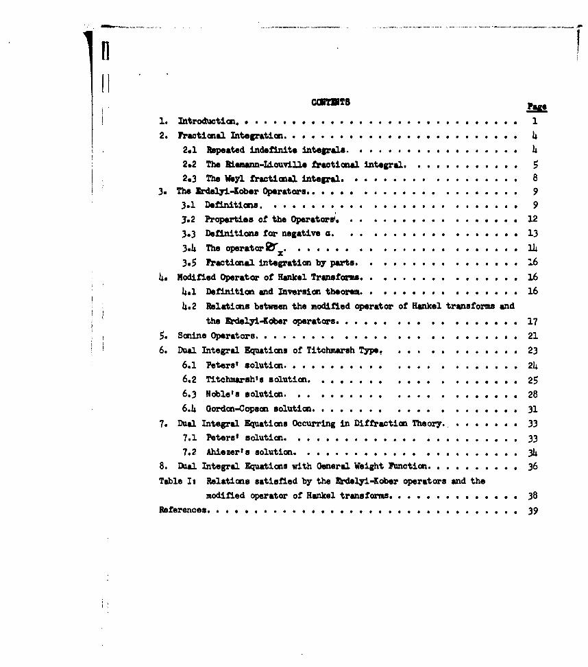
2. Fractional Integration.. . .... . . ................

2.1 Repeated indefinite integrals. ... ... ..... ...... 42@2 The R.ismmn-Liouville fractinl i.lnttegr .. roo......... . 5293 The Weyl fractional integral ... .. .. . ......... 8

3. The Erdelyi-Kober Operators... . .o o * . .#. . . . . . ..0. . ... 93.1 Definitions . . . . . ................ . . 9

3.2 Properties of the Operatorn. .. ........ ... . 12

3.3 Definitions for negative a . . ........... .*• • 133.4 The operator x ..y . . .o . . . . . .- . . . . . o .. . 14

3.5 Fractional integration by pazts ........ .......o 6

4. Modified Operator of Hankel Transfoms... ......... .. .. . 16

4.1 Definition and Inversion theorem . . . . . .0. . . . . . . . . 164.2 Relations between the modified operator of Hankel transforms and

the E'deyi-Kober operat ors ...... ........... 175. Sonine Operators. o . . ... ... . . . .. . . . . .. . 21

6. Dual Integral Equations of Titchmarsh Type. .9......... e23

6.1 Peters' solution. . o o . . . . .... . . . .. . ... .. . 24

6.2 Titchmarsh's solution. . . • . . o . .o. . . . ..0. .. ... 25

6.3 Noble's solution. . o ..0. . . . . . . ..0. . . . . . . . 28

6.4 Gordon-Copson solution ........ .... . .. .. .31

7. Dual Integral Equations Occurring in Diffraction Theory. . . . . . . . 33

7.1 Peters' solution. . . .0. 0 * . .. . .. . . . . * . .. .. 33

7.2 Ahiezer's solution . . . . . . . .. .. . * . .. ... 348. Dual Integral Equations with General Weight Function. . . . . . . . . . 36

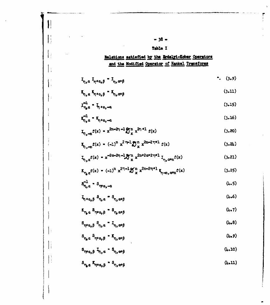
Table Is Relations satisfied by the Irdelyi-Kober operators and the

modified operator of Hankel transforms .. ............ 38

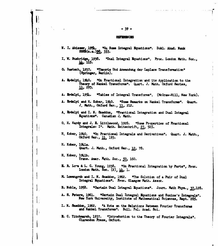
References. 9 e . e * e e * a e * * * * * & * 39

LUOTURS (YI JRACTIOMIA MU3TIrz

AND MJAL DMINUGL N~ATIONS8

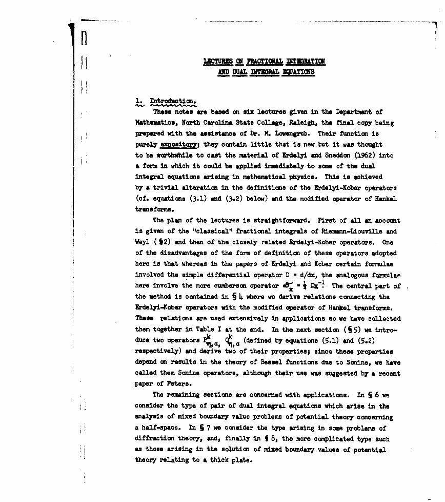
1. Introfdution.

Tb.se notes are based an six lectures given in the Department ofMathematics, North Carolina State College, Raleigh, the final copy being

prepared with the assistance of Dr. M. Lowengrub. Their function ispurely exmosait ;y they contain little that in new but it was thought

to be worthwhile to cast the material of Erdelyi and Sneddon (1962) intoa form in which it could be applied itmediately to some of the dualintegral equations arising in mathematical physics. This is achievedby a trivial alteration in the definitions of the Erdelyi-Kober operators(cf. equations (3.1) and (3.2) below) and the modified operator of Hankel

transforms.

The plan of the lectures is straightforward. First of all an accountis given of the "classical" fractional integrals of Riemann-Liouville and

Weyl (*2) and then of the closely related Erdelyi-Kober operators. Oneof the disadvantages of the form of definition of these operators adoptedhere is that whereas in the papers of Erdelyi and Kober certain formulaeinvolved the simple differential operator D - d/dx, the analogous formulaehere involve the more cumberson operator a 8 DI The central part of

the method is contained in S 4 where we derive relations connecting theErdelyi-Kober operators with the modified operator of Hankel transforms.These relations are used extensively in applications so we have collected

them together in Table I at the end. In the next section (S 5) we intro-duce two operators P.,k , (defined by equations (5.1) and (5.2)respectively) and derive two of their properties; since these propertiesdepend on results in the theory of Bessel functions due to Sonine, we have

called them Sonine operators, although their use was suggested by a recentpaper of Peters.

The remaining sections are concerned with applications. In § 6 weconsider the type of pair of dual integral equations which arise in theanalysis of mixed boundary value problems of potential theory concerning

a half-space. In 6 7 we consider the type arising in some problems ofdiffraction theory, and, finally in 1 8, the more complicated type suchas those arising in the solution of mixed boundary values of potentialtheory relating to a thick plate.

!f

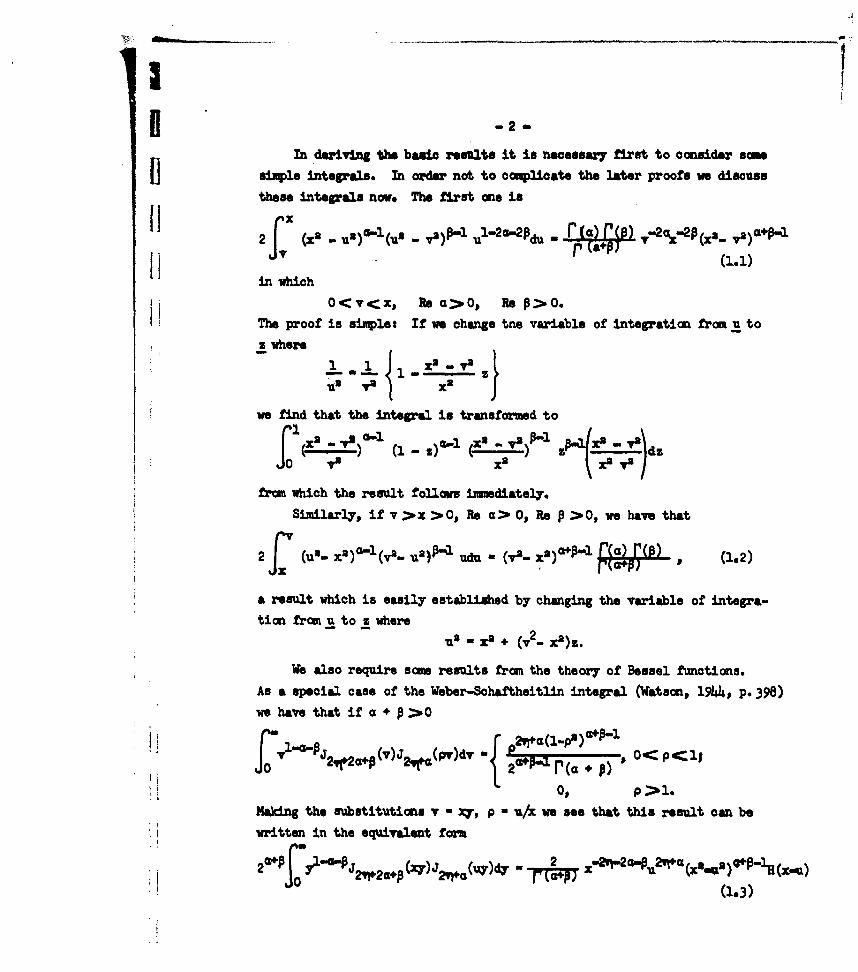
In deriving the basio results it is necessary first to consider sameshimle integrals. In order not to complicate the later proofs we discussthese integrals now. The first one is

IIx(xs . ua)a.,(u . ,)P-l ul.2a.i2. = ' () P) ,..2%(-2p(xa- .)a*KI (1.1)

in whichO<v<x, Re a>0, Re P>0.

The proof is simplet If we change tne variable of integration from u to

s where1 1 I .us V2 X2

we find that the integral in transformed to

f a V2a- 1 -) (S- a- £a _l m V2~) (l - • a~ dza Xa

from which the result follows imediately.

Similarly, if v >x >0, Re a> O, Re • >0, we have that

2f (un. xa)a-l(a-. ua)P-l udu (V2. x2)d+P-l • rfa) r , (1.2)

a result which is easily established by changing the variable of integra-tian from u to z where

us = xg + (v 2_- x)Z.

We also require some results from the theory of Bessel functions.

As a special case of the Weber-Sohaftheitlin integral (Watson, 1944, p. 398)we have that if a + P >0

r-1. J.20'" ,ft2c+P(v)j J (pv)dv Op1- - <P 1

0 , p >i.

Making the substitutions V - xy, p u/x we see that this result can be

written in the equivalent fora

'Pj vl"a'PJ 2 12 .+(xy)j 2 ,(.(Uy)d r (1.)(a-(7(1.3)

where H denotes Heavisaide'sa unit factione

A wenlmous result in the theory of Bessel fuwtions in Sltnt.ofirst integral

SmV*l )f v 0 2 +

"2" 2 J f A (a sin 0)sinIJ1 0 oo2v+1 o do.

(Watson, 1944, P.373). If we make the substitutions x - yx, sin 9 - u/xwe find that we can write this result in the form

o~ (x"- u2)v J,(uy)d - 2vxll÷v1 y"Olr(v + 1).ý,÷4l(xy) (1.4)

SonineIs second integral states that if Rev? Re I > -1,

No(+, 22).4, t÷i J (x)J, a, (t2+ s2)] dtf( 0)

- a VrzV(a% ii0 v ~ V (aS X2J H (a.4J,

(Watsons .1944, p. 415). The substitutions t V(t a- go), .I, --transform this equation to

aV. 2 )Jv -jr - - ÷iJI,• / (, 2 2) J (a,)dC

"ax• Y " z"'(am- xJ)jr Jr [ a 4 (A&" xs)j H(a - x), (1.6)

provided Rev > Re r*" -l. If we now divide both sides of this equationby x and let x tend to zero, we find that

( v- ) ,'1+"• J (av)d- - 2,"'f(v - r)a&'," Jr(a,), (1.7)

provided that Re sa 7O, Rev Re r>Rejv-..).

If we apply Hankel's inversion theorem to equation (LO.) we obtain

the equation

XO+ - ,2 X2i•(', - ilk - [ z (as- x,) J,((xt),dx

IaV 041t(ts+u3) 4 V Ja /(tX+ u')j , (Re v > Re -7 1). (1. 8)

m4m

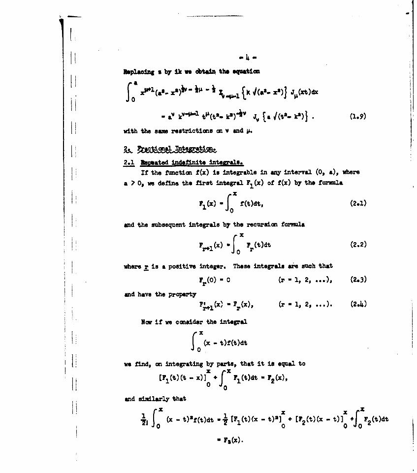
Replacing s by 1k we otai the epatien

0, tol(as si))v -il - p.i X2 .'.z)] J,,(xt)dxa .-" t.(ts- k2)+ J,, a., '( k). (1,9)

with the same restrictions on v and p.

~~? c Ia a nt o ýati p.

2.1 Rm•rated indefinite intearals.

If the function f(x) is Integrable in any interval (0, a), where

a ) 0, we define the first integral Fl(x) of f(x) by the formulaX

1', x) -of f(t)dt, (2.1)

and the subsequent integrals by the recurisi forwila

y.e(x) fX 7(t)dt (2.2)

where is a positive integer. These integrals are such that

Fr (0) - 0 (r - .,2, ...- ), (2.3)

and have the property

F ,.1(z). • •), (r 1 1, 2, ... ). (2.4)

Now if we oansider the integral

Xx - t)f(t)dtJo

we find, on integrating by parts, that it is equal tox ixp (7 1 (t)(t - X)]0 *f J F(t)dt -P,()

and si•ilarly that

I! 1 xx x

o (x - t)"f(t)dt - T1 .(t)(x -t)2J + [7 2 (t)(x " t)] OF 2(t)dt

M (x).00

[1

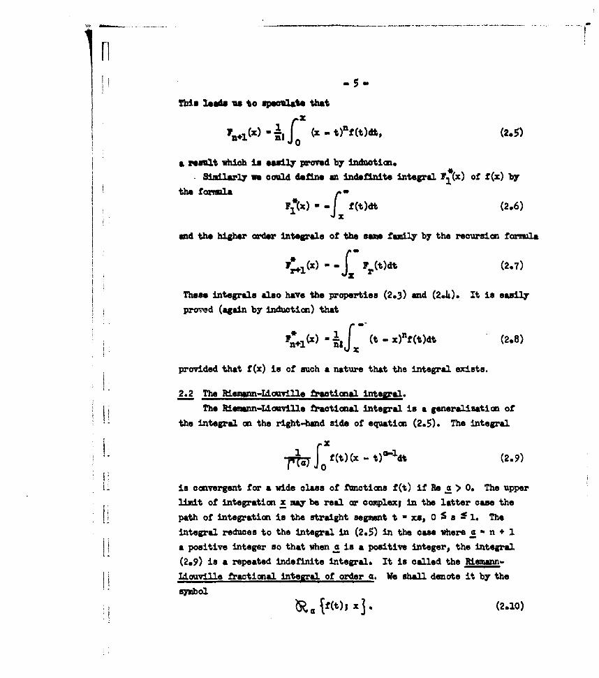
-5.Thin leads to b peclase that

ip,1 (X) (x - t)n,(t),,, (2.5)

a •e•ult which is easily proved by inductim.

Similarly we could define an indefinite integral Fj(x) of f (x) byeformla F•(x) - -f f(t)dt (2.6)

ix

and the higher order integrals of the same famil2y by the recursion formula

7r4,1 (X) f- F r(t)dt (2.7)

Thes integrals alo have the properties (2.3) and (2.4). It is easily

prove~d (again by induction) that

2.2 The Riemann-Liouoville fractional integral.The Riemann-Liouville fractional integral in a generalization of

the integral on the right-hand side of equation (2.5). The integral

S ff(t) (x - t)O1 dt (2.9)

is convergent for a wide class of functions f(t) if Re a > O. The upperlimit of integration x may be real or complexI in the latter case the

path of integration is the straight segment t - xe, 0 a•S sI. Theintegral reduces to the integral in (2.5) in the case where a - n + 1

I a positive integer so that when a is a positive integer, the integral(2.9) is a repeated indefinite integral. It is called the Riemann-

Idouville fractional integral of order C. We shall denote it by the

symbol.ýf Wf I x3 (2.10)

II- -I

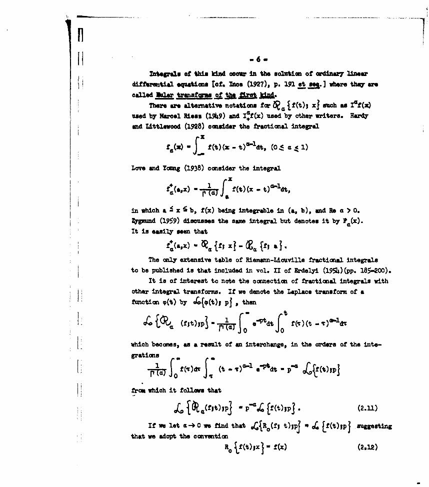
nt•grpoj of this kind oowm in the solution of ordinary linear

differential equations [of. Ince (1927), p. 191 at M.] where they are

called Valer tranufrms of Ai1There are alternative notatiouns for if j(t), I su xch as 16f (z)

used by Marcel Riess (1949) and I1f(x) used by other writers, Hardyand Littlewood (1928) omielder the fractional integral

nwhicha(zb - f(t) (z -b) "eldt, (0 ,, 1)

Lv and Yoang (1938) consider the integr.al

f a (so) M7 f(t) (x - t) aldt,

in which a < x 6 b, f (x) being in'tegrable in (a, b),, and Re cL > 0.

Zygmund (1959) dibcusses the ,anme Integral but denotes it by C(x).It is easily ueen that

L~~fand~ if¶,{:Z;::rz:2:ja4

The only extensive table of Riemann-Liouville fractianal integralsto be published is that included in vol. II of Erdelyi (1954)(pp. 18,.-200).

It is of interest to note the connectim of fractional Integrals with

other integral transforms. If we denote the Laplace transform of a

frnction p(PM by .r.{.(t), p] , then

which becomes, as a result of an interchange, in the orders of the inte-

grations

i f (IT) & (t-r a-Ptt-p4if(~p

from which it follows that

If we let a-+0 we find that &{Ro(fj t)ipJ " oC (f~t) ip suggesting

that we adopt the convention

R. z) (2.12)f~x

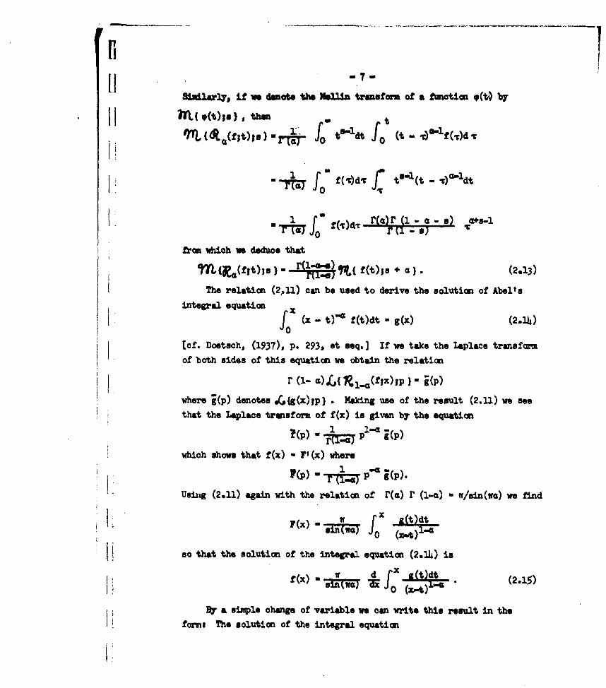
8liularlys if we denabe the Ne11in transform of a f~mot±im 4(t) by

Xthen

t J0 td f 0 (t, - rafdv

1 fC(l)dr f t"1 (t - r -d

1 4 f0 f(¶)d-rrar¶ ) c~-&as which we dedoce that

M7•l(•(flt);s " - f(t)r•. (•), (2.13)

The relation. (2.,n) can be used to derive the solution of Abel's

integral equatio. f x ( - t)"a f(t)dt - g(x) (2.114)

[cf. Doetach, (1937), p. 293, et seq.] If we take the Laplace transformof both sides of this equation we obtain the relation

r (1- a).G{ _.l(flx);p }- j(p)

where j(p) denotes oG•g(x)lp) . Making use of the result (2.n) we see

that the Laplace transform of f(x) is given by the equation

•(p) P, i(P)

which shoh that f(x) - F, (x) where

F(P) "7 P-a i(P)"

Using (2.11) again with the relation of r(a) r (i-m) - f/sin(wa) we find

I. F(x)- sfo•u( J0so that the soluticon of the integral equation (2.114) is

By a simple change of variable we can write this result in theforms The solution, of the integral equation

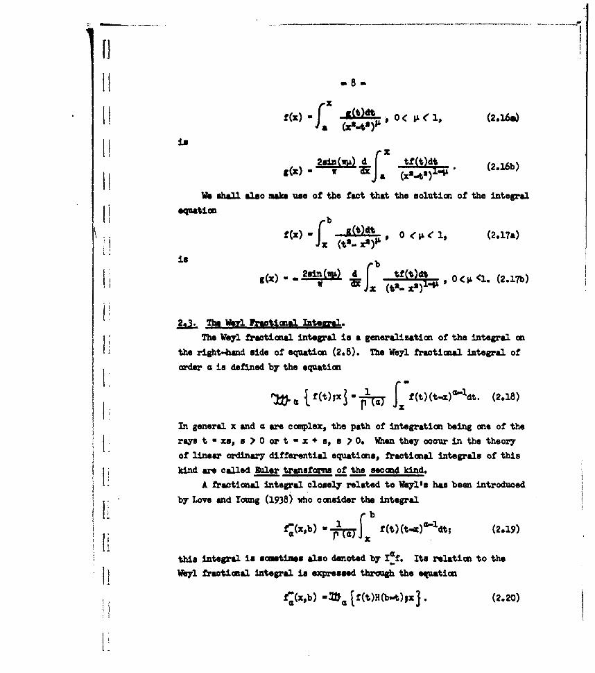
II -8-

IN (O,..) 0o < O l, '1 (2.16W

H fa 2i(uit)o

26in gWO d w Eja (2.16b)

We shall also make use of the fact that the solution of the integral

Ii ~equationbf!) l(t'. x')• ' 0 c •& ( I, (2.17a)

ii Cb

I: ~ ~ TheWy f~at nl f ntegal&i a generalisat•ion of the integral oni the right-hand side of equation (2.8). The Weyl fractional integral of

order G is defined by the equation

fi (f)_ ttdt.0-CA is dt (2.18a)

Ingeneral x and = are comple, the path of integation being oe of the

Iraystn- a, s 0 or t-x+s, s 0. Whetheycocurin thetheor

S~~~kind are called h~le...r transforms of the second kind.

in f

A fractional integal closely related to feyl's has been introduced

g (x b 1< pb f<)(u1.t (2.19b).li~2. The Lo e l andSA I~g(98 h osdr bh ntegral

This integral is mtiaen also denoted b lf I t. ezlation to the

! W~ey1 fractional integral is expressed ty the equation

if~xb in(t) H f (t) (tx ) s.t (2.20)

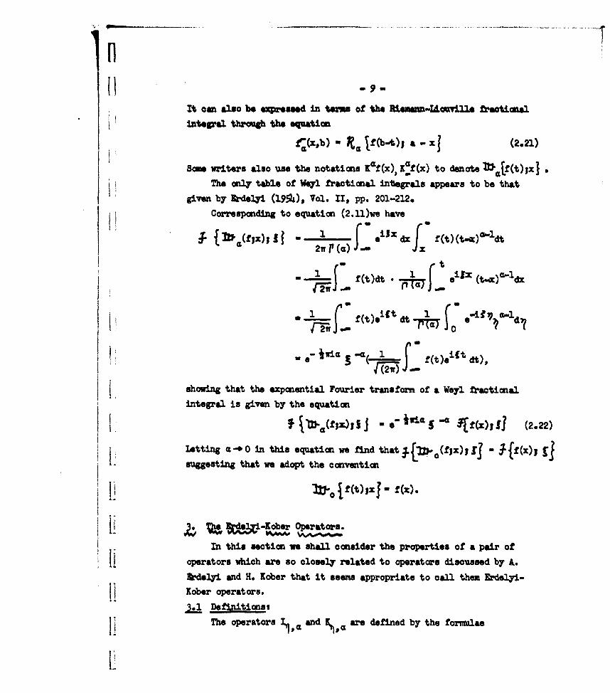
It can also be expresmd in t of the liseann-LiouriU. fraotionalintegral through th quation

f*(x,b) - f f(b-t)j a - x ~ (2.21)

Some writers also use the notatiouns I f Cx),x Kf(x) to denote Wcjf W)Ix1The on•y table of Weyl fractional integrals appears to be that

given by Irdelyi (1954), Vol. II, pp. 201-212.Corresponding to equation (2."1)we have

(f x I eisx ( )( . ) -Ia 2w___ P (a L dxJ f f(t) (t-Z),1 dIt

" f(t)dt e* (t-x)U'ldx

a e. .-. j f(t)e it dt),r!-t fj..M

Sjshowing that the exponential Fourier transform of a Weyl fractional

integral is given by the equation

I. ~j.~(~z)S a- 4 I* ff(z), (2.22)

Letting a -*0 in this equation we find that ~{.(fux)i I~ f- {X); Isuggesting that we adopt the convention

1'~ W0 f(t) Ixj f (Z).

[~ Ad-K ber Oprators.

In this section we shall consider the properties of a pair of

operators which are so closely related to operators discussed by A.

Zrdslyi and H. Kober that it seems appropriate to call them Lkdelyi-

Jt Kober operators.

3.1 DefinitionsIi The operators and , are defined by the formulae

101tWi

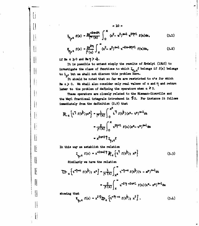
fLZ (X2 _ M2)0-1 U2l1*1 t(U), (3.1)

f Wj fx 2X21' f (u2- z2) 01 U-*~ f (u)du9, (3.2)

Iiif ReG.aj0 and Is >uIt is possible to extend simply the results of Erdelyi (1940) to

investigate the claus of ftmntions to which T.af belongs if f(x) belongs

to L, but we shall not discuss this problem here.

It should be noted that so far we are restricted to a's for which

Re a >0. We shall also consider only real values of a and 7 and return

laUtr to the problem of defining the operators when a 1 0.

These operators are closely related to the Riemann-Liouville and

the Weyl fractional integrals introduced in 9 2. For instance it follows

I immediately from the definition (2.9) that

I (4 I 21 f uX'11 f(ti) (X2_ t2) 1du-

0i -r z242 0

In this way we establish the relationx

I SLf (x) - :X-2w f 4 ; (3*3)

I Simi ly we have the relation

It I a1' f (ti)* 2 " af(), (tJ 3e)7 a- l

Ii 2 pua f -2 1 ..2a4~l f(M) (U2_ xl) a-du

{Is h o w i n g t h a t f x 2 q , a I -a f t ) x j( 3 4

[31Sam particular oae ae of intwest. If we let a.-0 and make

use of the eqpatci•s (2.12), (2.23) we see that the ocavmnt±ia

1bOf (X) - f (x), Kof(x) - f(x) 35)

is marely a restatement of the conventio

P- f()IX - f W), U00 {t (t); X) - f(x).

fwrther, if we put - 0 in eqiatime (3-.3) and (3.4) ie obtain the rela-t i m e 0 3,o a g ) _ - 2 a a, Mt i ) , x 2 ) . K o ., f X ) -: Gf ¢( 4 ) , 1 X

(3.6)Because of the relatiazs (3.3), (3.*) it is a simple matter to use

the tables in Nrdelyi (1954) to calculate I f (x) and K f (x) for any

presoribed ftnctian f(x). For exampleg ift

f(x) - x2P(x2 + o0)Y,

then

Nowq, from entry (9) on p. 186 of Vol. II of Erdelyi (1954), we know that

if a >0,, P+ q÷ > 1 0, then

.k+k~o)~ 02 yxa~p* T(8Ao,vl) a ,*gl 9*143--I r (,MP 1+ 1)

if Irg X/•2 1 < W. It follows immediately from equation (03) that for

II this f( m) 'x P r p 1o)P . l a + n 1 21 ! fx) 0 ~r(a + V),n 1) x2

if Iang x/cl ~I <w.;t is often a simple matter to calculate I.,, af directly. For example,

since

ii~it follows that

L - (a .. ,&lp .1F+*( "1,...,bq, a÷1÷l3 xb)

(3.7)

U .. 12wSie q denotes a g=umelsed kbnpegecntrio function.

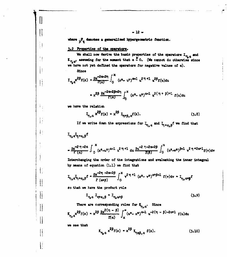
3@2 hrcerties of the 92e1O ..We shall now derive the basic preoptioes of the operators Ia and

IKn, assuming for the maent that a t 0. (We omnnot do otherwise since

we have not yet defined the operators for negative values of a).

since

I~~ x•p (Z 2o6- (xj- ujl)*- u211* _2f(u)du

, xp z 2u-2ta n (xa- uO)a".1 -a2 (T + P)+l f (u)du

we have the relation

, x02 pf (x) - x2 p %3ý,+*,f (x). (3o8)

If we write down the expressions for 3 a and ý+,f we find that

2j 71-a f 0 (x2_uS)"'-l u2 71 +1 du 2u-2 tj-2 0(ýNAP 2, 2*lrvdr (a AU

Interchanging the order of the intep'atiais and evaluating the inner integal

by mans of equation (1.1) we find that

* ~~~~~2xj2' -2a.-2p x v~ ~ ~ d

I Ii ~ - r (ct+p) (x-*)P0so that we have the product rule

There are corresponding rules for I Since

K2 f (X) a X x2 (i jf~ a -13 ) u2(yi - p)-2a'1 f (u)dux

we see that

II K • x f( x) " • ,p • fc x). (3. 1 0)

iiaf(X.(-0

I]

H -13

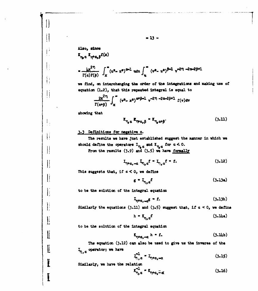
+ x~~,,, nKfeef•z)

, f (us. x2),. Wu (vs uO)K V'e4 Tj .-2.-2p*r(co r(p )f

we find, on intergc the ador of the integrations and making use of

K equation~ (1*2),0 that this repeated integral is equal to2, •2,q 4 (va- xa)0,p,.I vw.T .2a2P+1 f(v)dvr(cc+p) i

showeing thatSra nr,-K 0'row (3.11)

3.3 Definitions for negative a.

The results we have just established sugpst the manner in which we

should define the operatore I and K for a-O.

From the results (3.9) and (3.5) we have £asual.y

This suggests that, if a < 0, we define

9 w ýpf (3-13&)

ti to be the solution of the integral equation

* f. (3.13b)

Similarly the equations (3.11) and (395) suggest that, if a < 0, we define

h - K1omf (3.J24a)

to be the solutioi of the integral equation

The equatiton (3.12) can also be used to give us the inverse of the

I! L,,operator we have - (3.15)

Similarly, we have the relationfo , (3.16)

114

S1 now introduce the operator

x Vto obtain relations from which we derive formulae by means of which we

11may calculate ISa and 11Cwhen a 0O.By the definition of the • operator we have that

In.a It" -1" t2+ I f (t);x X

.( t2)'-1jl tr +v l (t)dt.V r(a) o t

Applying the formula for integrating by parts we find that the integralon the right-hand side of this equaticc becomes

"2 {1(xt2)aj-I t -l 2n+ v +1 f1

+ (a-l) f( X " t(X2_ t v1 f(t)dt)

r~ez) oCW%01,, t n÷ f(t)dtrf....i) 04

lI showing that

Lý it, t t2n4.v 4.1 f (t) Ix x- ( t- 2 y) -1 j7nlt+v f (t)Ix)

If we repeat the process n times we obtain the relation

E , t"2 'I'1 trn t2 n+ 1 f(t),• -2n 2--t2, t + f (t)Ix 1. (3.18)

Li Making the substitution a = n, replacing i by in- n, and making use of

equation (3.5) we find that this result can be written In the form

i I' (-n ' + 2n'Z n tn+ v+1 f(t)jx} - x n'2 271 + Vf(x)

j anduasing the relation (3.15) we have the relation

IvM~ x2n.-2- f(x) W x~n-2Ti -ZBnx x2n11v +1 (3.19)Iýn

LI - 15 .

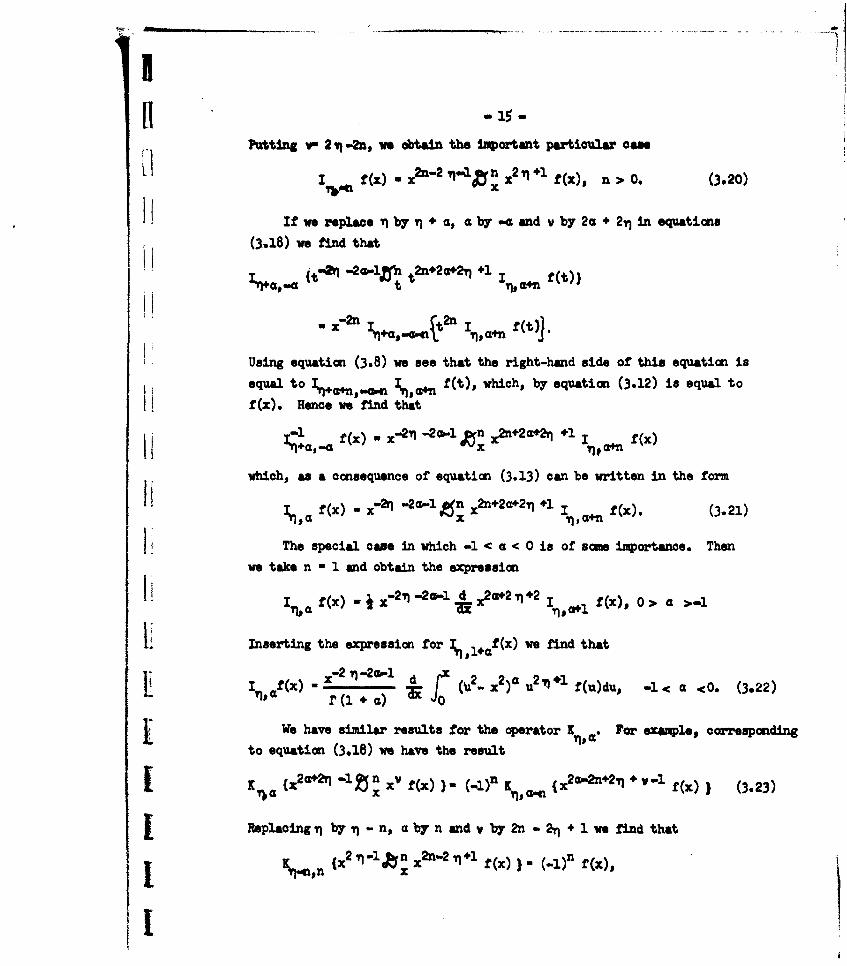
fttinag v- 2, v.-2n, we obtain the Important partioulazr ame

I f (z) - z- 2 Tj1j n x21 *1 f (x), n > 0. (3.20)

If we oeplaoe ",1 iby + a, a by -a and v by 2a + 2, in equaticon

(3.18) we find that

i',4 {t-cn -2a-ln t2n+2" +1 1 f(t)}

Using equation (3.8) we see that the right-hand side of this equation is

equal to •+a+n,,-on Ila+n f(t), which, by equation (3.12) is equal to

f(x). Hence we find that

-i (x) - X-' -2a-i In x2n+2a+2y 1 1 f(x)

which, as a consequence of equation (3.13) can be written in the form

, f(x) . e-n -2a-1 n x +2a42yI ,1 1 f(x). (3.21)

I The special case in which -1 < a < 0 is of scm importance. Thenwe take n - 1 and obtain the expression

L. I . f(x) "a e 1 ,1 f(x), 0> a >.l

LInserting the expressioni for ý '1+Q f(x) we find thatI•' ) "r-2I~-2a.-1 d (V2 _ x2 )a u2 , 1 f(u)du, -1< a <. (3.22)

We have similar results for the operator K X . For example, oomvespu ding

to equation (3.18) we have the result

I K {x2 4 2Y1 -1 p n xv f .(x)n x2a-÷2.n + ,v--1 fMx) (3.23)

j ReplacingiT by- - n, abyn andv by2n- + 1 we find that

K. n -1 & n (x) (_,)n f(x),mmn x

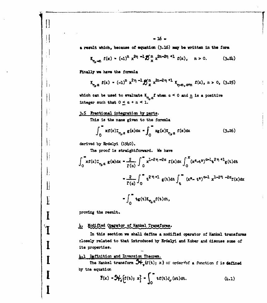
m 16-.

a result which, because of equation (3.16) mr be written in the form

f(x) - (-1)n x - n x'-q ÷. f(x), n > 0. (3.24)

Finally we have the formula

Kilo a f (x) - (-I)n x -1 Ze, x..2!- +1 , f(x), n > 0, (3.25)

which can be used to evaluate Kil f when a 0 and n ise a positiveinteger such that 0 < a + n -c .

395 Fracotional integration by parts.

This is the name given to the formula

f0 xf(x)Ia g(x)dx "fO* xg (x)K , f(x)dx (3.26)

t ~derived by" Erdely_ (1940o).

The proof is straightforward. We have

r(c) o t

uftg(t)r.. f (t)dt,

proving the result.

"J4. d Opsrator of Hankel Transforms.

In this section we shall define a modified operator of Hankel transforu

closely related to that introduced by Erdelyi and Kober and discuss some of

its properties.

4#1 Rgfinition and Inversion Theorem.

The Hankel transform .4v((t); x) or order-of a function f is definedby the equation

?(

I,!

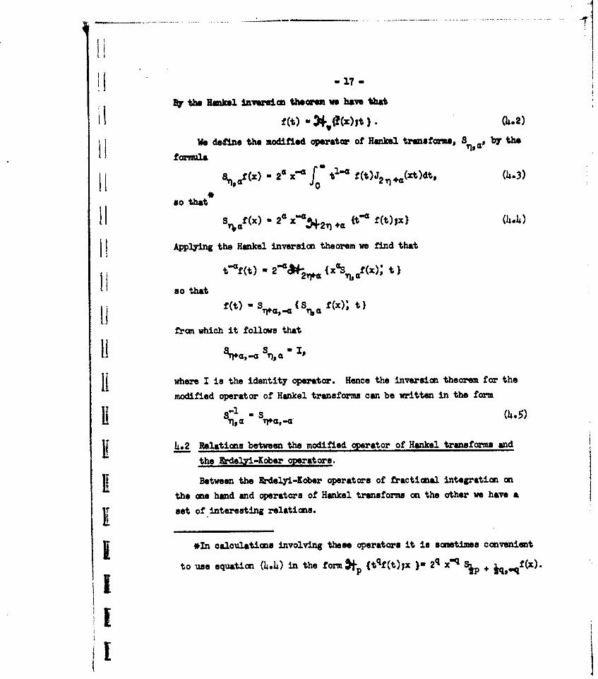
-17-Sthe Hnol Inversion theoreo we have that

St•he R ¢ik- (t) ON). ÷(it. (¢4.2)

ljWe deftne the modified operator of Hankel. trmnsformse, 8 T19 by the

formila,

87 G(x)-22x' t1a,(tdf43

ttf (t) - 2'tJ%", ,f t(x); t( )

so thattf (t) - 2'r~a&4- {xSa f (X) " t

from which it follows that

sI+a -a,-G S7", M"IV

11 where I is the identity operator. Hence the inversion theorem for the

modified operator of Hankel transforms can be written in the form

Iiq -. 71+a (14-5)I 4,_2 Relations between the modified operator of Hankel transforms and

the Prdesyi-Kober operators.

SBetween the Erdelyi-Kober operators of fractional integration on

the one hand and operators of Hankel transforms on the other we have a

set of interesting relations.

*In calculations involving these operators it is someties convenient

to use equation (4.4) in the form p (tqf(t)jx )- 2 q x• S~p + , •f(x).

Iiii

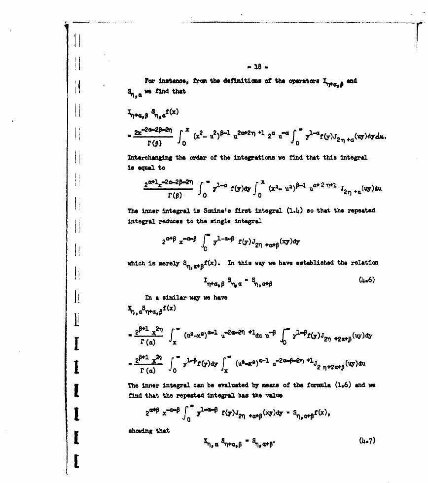
for instance,, fromi the defzinitionsa of the operators q4. P4S1 , 6 we find that

Interchanging the order of the integations we find that this integral

in equal to

20f 1-2OI2-2 ",y-a f(Y)dyJ (xa, n,)p-i ua*2,3

r(p) fo . o (2n ÷ji)du

The inner intera.l is Saiine's first integral (1.4) so that the repeatedintegral reduces to the single integral

2aM+ xs-O-P TL~ yl-".o f (y)J21++ (Cx7y)(0

which is merely STI f(x). In this way we have established the relation

'. I,.+Q,. Sr, a - 'T, o.p (4,.6)

h In a similar way we have

W - I "1"Pf (Y)c, (,,..),,-d ,, j- y-en,, ... 2,,, (vT,)du

r (a)

The inner integral can be evaluated by means of the formula (1,.6) and wefind that the repeated integral has the value

I20" x-- £o. yl"OP" fby)J21) ,4.,(x47)dy - S,.px,

showing that'%,r •rio,p % p"%• •

[

•00

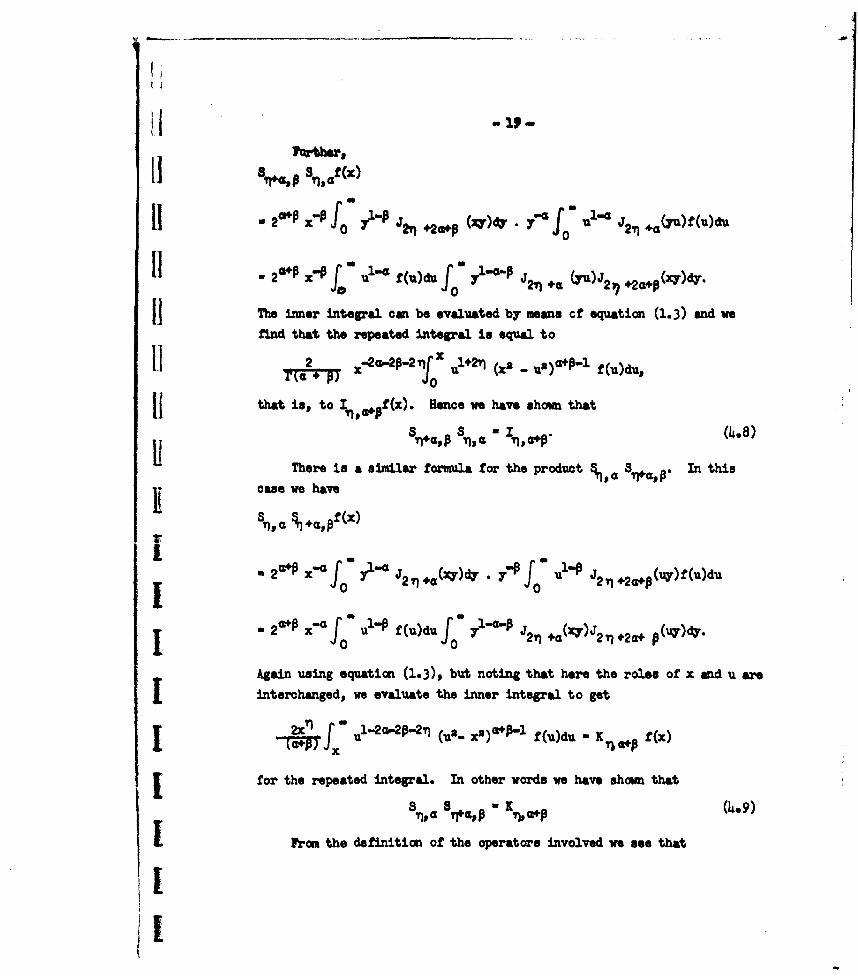
11 -

II 2G*P xi -P f Yl-P J2, ,,+ (xy)dy. yý' fo uls' u 2, 1 +a(yu)f (u)di1

. 2CP x-Pf - :' f(u)du yO - J (yu)J•-, ()dy.

jThe inner integral can be evaluated by means cf equatio u (1.3) and wefind that the repeated integral is equal to

Ii 2 X-2a-2P-2,fj, U*2n (x2 - U,)U+A-l f(U)du,

that is, to defniox). Hncee we have thosn that

I The. s a rn, C&P (4.8)Threisasimilar formulafo the poutý L'14.P In this

Ii %,OU %+CfLx)

u2xC fy J 2 -P (~4 f fu J2 ,1,2 ,+P(uy)f(u)du

a 2c" xl-aP"J f(u)du fo 71-a- J2,n +ax~2T+a p(uy)dy.

Again using equatioun (1.3)p but noting that here the roles of x and u are[ interchanged, we evaluate the inner integral to get

IxT f ul2mpT (u2- xa)+P-l f(u)du -K f W~x

[for the repeated integral. In other words we have showia that

S no a m#LPwKr + (14-9)

I From the definition of the operators involved we see that

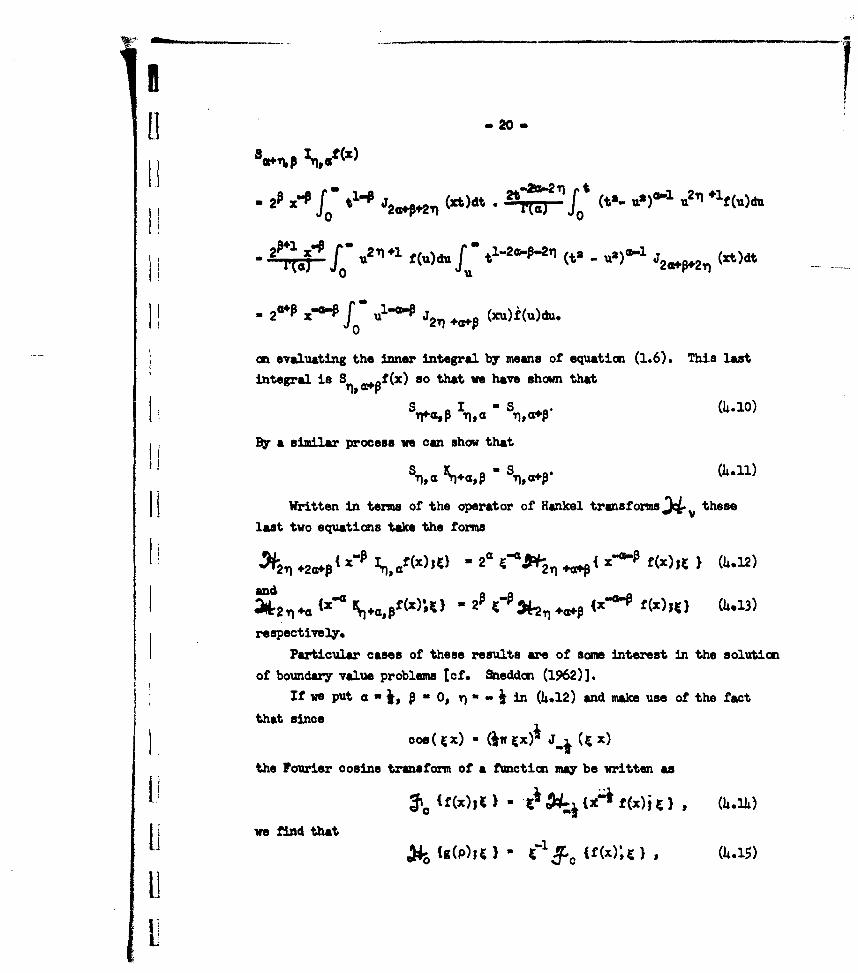
Ii -20-

S2P x"P •-20,,.P + (2c)dt. rM-j t (t'e- u")a-l U2Tj *lf(u)du

2P' " &I - .2 -n1 f (u)du (t2 _ u2)4-1 j2 (xt)dt

I on evaluating the inner integral by means of equation (1.6). This last

integral is S n,,+Pf(x) so that we have shown that

I tai By a similar process we can show that

iWritten in terms of the operator of Hankel transforms theselast two equations take the forma

I ~•21"1 ÷€ x••,and ~)• 2P3 C' 3ý2 ,+•,p (x-C-P f¢(x) It (4.13)

respectively.

Particular cases of these results are of some interest in the solution

of boundary value problems tof. Sheddan (1962)].

If we put a - -, * -o in (h.12) and make use of the fact

that since

the Fourier cosine transform of a function may be written as

[ we find that it~ (gP)~ I f {(X)) (4-15)

1IiIj

I ~1

I - 21-

I! hx)-2"xK , IT) ixf %/Pf(x)dP'x'"(.8

g~p) *21 f.~ (fP) A. fJ 3 f 3X (4-16)

I ilaf we put =o, P = i 0 in (4. 13) we findthat

W_ (. (f ((p).•" ,, ,.o h(x) •t ) (4.17)

¢' (p .. ,)dp

h(x) - x (p)p (4I.18)

If we Put a - irot n 0 in (oe .12)we find that~ (3(P; C) 1(l158 (fx), W (4-.19)

wher (p 2S1, f 1(P) - P xf V(x2-z (I&.20)

and we (hax); eriv f %1 (x);•e e ne . 21)

is the Fourier sine transform of s(x).

KFinallY Putting amp 'n, 0 in(4.13) we find that

5. Sonine operators

We Shall now introduce two operators Pk and whxose two main

properties we shall derive by using &imine's second integral. For that

reason we shall call them Scnine operators.

We define P 'k by the equations

[xQk f fx t1l- J.{ k V(t2- x2) ) (t2" xg)c f (t)dt. (a > -1) (5.2)

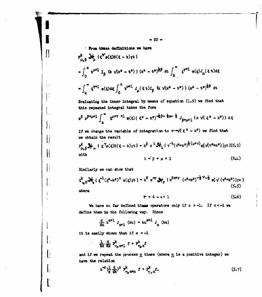
-22-

F rom tMses dtfiniticne we have

PX,, 4t V I/(x 2 ( - k)) It - ' 1 ~d

fk(

Evaluating the inner integral by means of equaticon (1.9) we find thatthis repeated integral takes the form

kP kf 4jp~~ ( 2)

If we change the variable of integration to % /"V( t2 - k2) we find that

we obtain the result

4XItY (JgH (,9- k); t) kP x rý(2k) '+)P (2k)Ij (-3

w x WP + 0 + 1 (5.4,)

Similarly we can show that

where (5.5)

e -8 mV + (5.6)

We have so far defined thwn operators only if a >-1. If a <-1 we

define them in the following way. Since

d ua+lj (ku) - kulc I J (ku)

it is easily shown that if a >-1

1~ d ,a pX f pk f

[ and if we repeat the process n times (where n is a positive integer) we

have the relation

IkLn 1 d,n

I

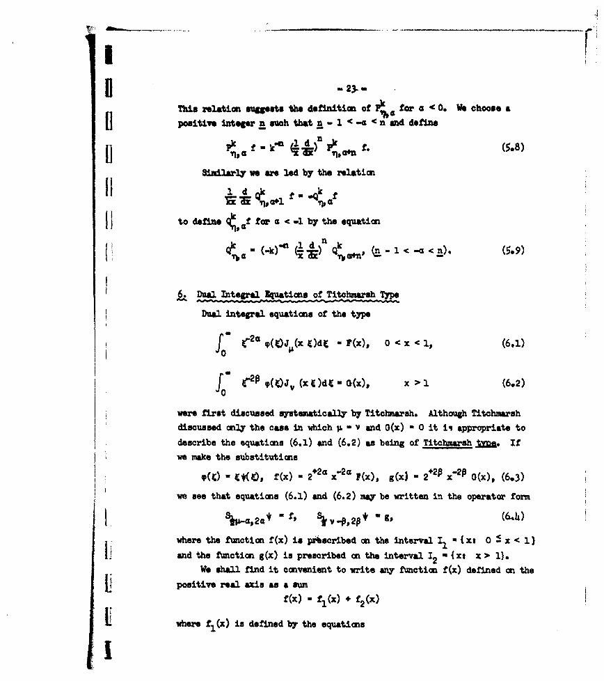
II -23.-

This relation suggests the definitiom off }- for a < 0. We choose a

Positive integer a such that n - I<-a <nand define

IIq dI~ plc f.

SMiila-ly we are led by the relatim

1 -dkQ • k =

to define f for a < -1 by•the equation

1d nk

Qu(1c) Q T Cý 1<-a n (5-9)

6. Dual Integral ,Uquaatins of Titchmarsh Type

Dual integral equations of the type

f W C2a c(C)JýL(x t:)dt - rP(x),, 0 <x < it (6.1)

f CIPowi (x C )dt - G(x), X> 1 (6.2)K o

0

were first discussed 8syteuatically by Titchmarsh. Although Titchmarsh

discussed only the case in which p - v and 0(x) - 0 it i'i appropriate to

describe the equations (6.1) and (6.2) as being of Titchmarsh _t. If

we make the substitutions

(C) -q F.v(, C f(x) - 2 2a "2 a ?(x), g(x) - 2 G2 x"2P 0(x), (6.3)

we see that equatioms (6.1) and (6.2) may be written in the operator form

I %lp-a,,2cz 1 - p '*v-P,2p* - g0(64

where the functicon f W) is prbscribed. on the interval Ii tx 0 :1 x '1

I and the function g(x) is prescribed on the interval 12 - {xt x > 1).

We shall find it convenient to write any function f(x) defined an the

positive real axis as a sumf(X) " fl(X) + f2 ¢(x)

L where fi(x) is defined by the equations

I

II °,

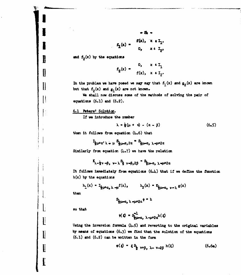
L(x). 9 x all,

0.9 x 0 12,

and 12(x) by the equat±ion

0, x I1II 2 " (x), x £ 120

In the problem we have posed we may say that fl(x) and g2 (x) ae known

but that f2(x) and gl(x) are not known.We shall now discuss some of the methods of solving the pair of

equatians (6.1) and (6.2).

6.1 Peters' Solution.

If we introduce the number

*-(P + V) - (a - •(6.5)

then it follows from equation (4.6) that

I ' - -2a " a, -p+2a

Similarly from equation (6-7) we have the relation

X-jv 4,, v- O v- ,.,2P " , .g÷2a

It follows immediately frma equations (6.4) that if we define the ftnoticn

h(x) by the equations

h.1(x) - j4+')ýf (x),t h 2 (x) - Ki 1-e v g (x)

then•lpG,)• .b42a* h

so that

1'(• - 8•, 1 I X•÷J*G(•)

Using the inversion formula (4.e) and reverting to the original variables

by means of equations (6.3) we find that the solution of the equations

(6.1) and (6.2) can be written in the fom

9(4) - % v,, ) (6.6a)vphC

Ii

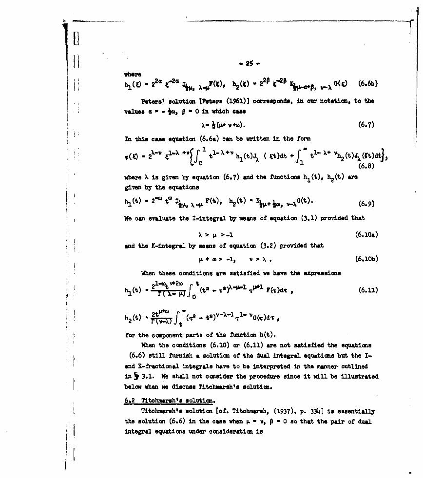
where 2a( t- 2 a '' ,7~(4), h2(4) 2 •2P e.p GQ•, .• ) (6.6b)

Peters, solution [Peters (1961)] coxrsponds, in our notation, to the

values a* - J o 0 In which 1ase

- V 4W). (6.7)

In this case equation (6.6a) can be written in the form

2"-v tl "- v'o tl'- h(t),, (. tt)dt + ltl '-+ h 2 (t)JptJdtj',(6.8)

where X is given by equation (6.7) and the functions h,(t), h2 (t) are

given by the equations

hl(t) - 2"0 F°-• , (t), h2(t) a K÷j .. ot).(69

We can evaluate the I-integral by means of equation (3.1) provided that

ad> th > -I (6 .10a)

and the K-int -al by means of equation (3.2) provided that

L + M > -I, V > X (6.10h)

When these conditions are satisfied we have the expressions

h_(t) - r2t f ) ¶-)X. b r(o)d, (6.11)

h2 (t) r"v ] ( 2 " tt) Xv-))tn vG(.r)d,

for the component parts of the function h(t).

When the conditions (6.10) or (6.11) are not satisfied the equations

(6.6) still furnish a solution of the dual integral equations but the I-

and K-fractional integrals have to be interpreted in the manner outlined

in 5 3.1. We shall not conuider the procedure since it will be illustrated

below when we discuss Titcbmarsh's solution.

6.2 Titohmarshts solution.Titohmarsh's solution [of. Titohmarsh, (1937), p. 334] is essentially

the solution (6.6) in the caue when I = v. 0 so that the pair of dual

j integral equations under consideration is

it

-2a -26 -efoffo •a ,€•., ¢(xOdC - ,¢x), x. S . ¢~6.13)

10fo 4p *(¢)J,, (•x)dt - G-•) x ( "2" (6.,14)

SIf we put lk - v,p O, 0 v-a into equations (6.6) we find that the

solution of these equations is

a(t)d t h+Ct)Jv.a(t)dt(6.15)

where h,(t) and h2 (t) are given by the equations

(t) " 22a t"2a Tiv ,-a (t) -%v .aaP(t) (6.16)

In the computation of h,(t) and h2(t) two cases must be distinguished

according as a is positive or negative.Case (i)s < t0 We suppose that n is the smallest positive integer for

which n ; -a. If a < 0, then by equations (3.1) and (6.16) we have

h(t) M 21+2at-v t . •a- D-I V+l F(•)ds (a < 0) v > -1)

and by equations (3.25) and (6.16)

h2 (t) .2-l~ tv20 -X tf (T - t2)2*n- Tlv(rdS"~~ r(a Z n) t ft )+- • vo••

Substituting these expressions into equation (6.15) we obtain the solution

2 1+a +a 1 l 1 +I

+ (-nlar - L V tVyGJ i t) dtj~n t ,2 )an 1 r-vG(rdr (in a + 1n) /t-

(6.17)valid for -n <a <0, v >-1.

In the special case in which O(') - 0 we obtain the expression

.(P) W (2 t)1-a f: F.tt 1- Yo . 2)-4-1 el0 tY.)dY0 0 (6.18)

valid for a < 01 this is Titohmarsh's solution.

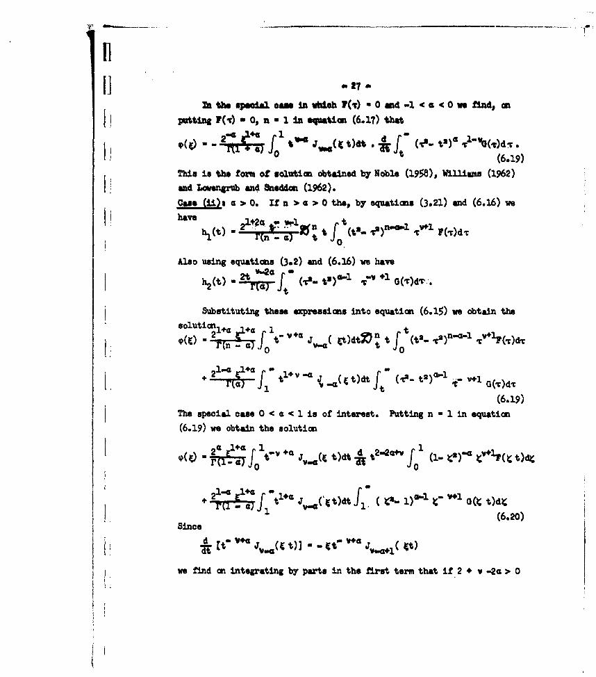
UI the speoial emwin idndh io (- v) 0 and '-1 - c 0 we find onu

Put~tinig N) - tn -1 Inhlqua~tzio(61)ta

2 1" ..._ , 1 t We J (C )dt . "gd ('tWO(r)d-T0 ft (6.19)

This is the form of solution obtained by Noble (3.958),, WilliaDW (1962)I ad W WL Ub and 8nedden (1962).

Cane (is i) a 0 0. If n > a > 0 thb, by equaticas (3.21) and (6.16) we

V ~ ~have t -I I f

Also uaing equations (3.2) and (6.16) re have

Substituting these expreusians into equation (6.15) we obtain the

solutionl+a ef a• (n) -- a o-t" v+d Jvi tt)dt:O n t t(t2_ T2)n-a-l Ty+'I(,)dr

- t/+ 21 1 $a ( td) " (,- t)C --1)

(6.19)

The special case 0 < a < 1 is of interest. Putting n 1 in equation

(6.19) we obtain the solution

I 24 1 (6.20)

Since

we find an integrating by parts in the first term that if 2 + v -2a > 0

[ - 28-

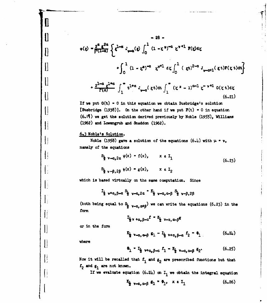
1 (1 - X•l)' •V4 dXf ( )2a Va ( )y(t) i

+ 2l ) 1+ Ct~t (.2 1a1CVlG t)dY.+ r~a) a

11 -1 -1(6.21)If we put 0(t) - 0 in this equation we obtain Busbridge's solution

tfluebridge (1938)]. On the other hand if we put F(t) - 0 in equation

(6.11) we get the solution derived previously by Noble (1955), Williams

(1962) and Lovengrub and &neddon (1962).

6.3 Noble's Solution.

Noble (1958) gave a solution of the equations (6.4) with IA v,

namely of the equations

Si v-a,2a (6.23)

1: ,2P *(x) - g(x), 2

which is based virtually on the same coMputation. Since

V~a"P--d Sk v-esa i -Qs- %~ v-P,2P

(both being equal to Pi vsaLP l we can write the equations (6.23) in the

form -

o r i n t h e f o r m % .Q , -p 1 1 j V % P a ' - * 1( 2 4IiK " g 1•, -I • -•, 12 (6.24)wh r Ii v + s% P -a fl ý Y V -a pa-p g2. (6 .2 5)

Now it will be recalled that fl and g2 are prescribed functions but thatf2 and gl are not known.

If we evaluate equation (6.24) on I we obtain the integral equation

K1 v,.a, a-. g1 "it x 9 I1 (6.26)

I]

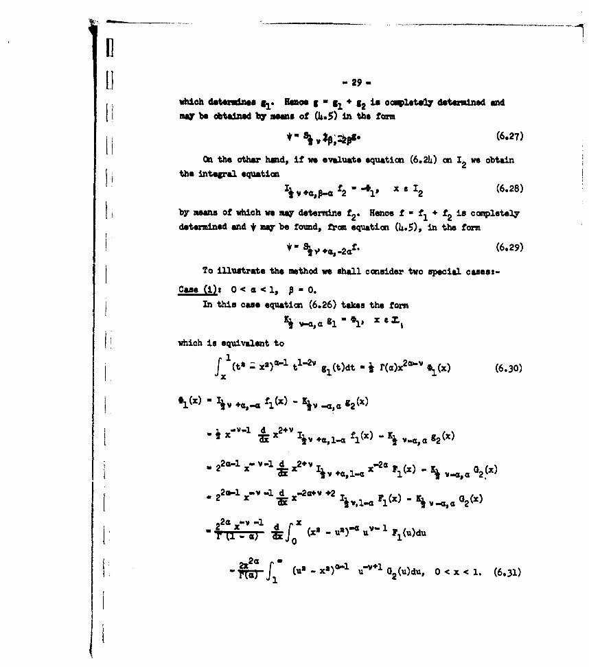
11 - -29whioh 4.ternines si. gowne g a , + g in cowqleteV. determined and11 ~may be obtained by means of (6&5) in the farm

¶4ru (6.27)On the other hand, if we evaluate equation (6.24) on I2 we obtain

the integral equation

Ii V.+t .Q f2 - V x 12 (6.28)

by eans of which we may determine f2. Hence f = fI + f2 is completely

determined and * may be foimd, from equation (45), in the form

(6.29)

To illustrate the method we shall consider two special cases:-

Case (.): o < a < 1, P - o.In this case equation (6.26) takes the farm

I* V-Qj a g•. = Oig x amS-

which is equivalent to1

fx(ta gl(t)dt - j r()x 0 (X) (6.30)

"9 3 4,-a fxl() -÷Iv -a,l a I(x)

x Kv-i d x2 +v-

I* V1 +a, 1-a flCK) -K1 , 92 (z)

2op-l v-1~ d x2+V K"2 - 0 (x

2.-1i -i d .20"E-2 K, *~* I-vi.a r(x) K v -,a02(x)

22a; K -1vdi df x(2-u)a UV ur 6) (x' - u'- ua) 'M(

2x2i-. f• j (uo - x2)"" u"÷1( G2(u)du, 0< x< 1. (6.31)

{1

w

-30

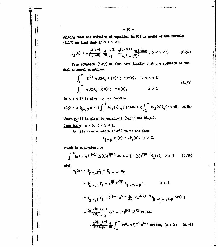
writing do= tew soutiam of equatim (6.30) by mean of the formula

(2.17)we find thxatifO0'<a5'1

£i(t) t..~ 0a <¶-) ,0' < 1 (6.32)

From equation (6.27) we then have finall3y that the solution of the

dual integral equations

fo es F(4)j ( x)dg -F(x), 0<x<l(6.33)1 . ()WJv (Cx)dt - G(x), x > 1

(0 c a < 1) is given by the formula

VW - C SiVOc g - I tg1(t)Jv( 4t)dt + f tG (tJ (4tOdt (6.34k)

where g1 (t) is given by equations (6.32) and (6.31).

Case (ii): a 0, O< b0< 1.

In this case equation (6.28) takes the form

IiV,p f 2 (x) - •41 (x), x I

which is equivalent to

X,(X2 t2)P-* fa(t)t 2 p+1 dt - - j r(p)x 2+% 1 (x), x> 1 (6.35)

with

!-2x) y1 (x - u) u"-p (2jx _1. _)hpuv (~ (I 1 (6.3)

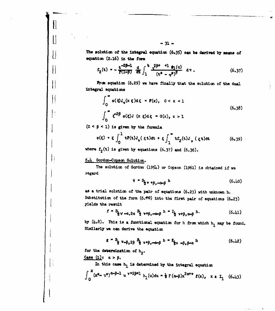
111[1 - 31-

The solution of the integral equatien (6.35) can be dewlved by means ofSequation (2.16) in the rtom

;r2 t) -2P1 d t 2P+ +1?(-)Wf, (t ? d¶. (6.37)

Fr'om equation (6,29) we have finally that the solution of the dualintegral equations

0 (6.38)

f c.p Q•)J (x C)dt - o~x), x >-,

0(0 < P < 1) is given by the fonimla

1 p.tj(ý~d f4

C~ f, V J't'tJ( td tf 2 (t)J, ( Pt)dt (6.39)where f 2 (t) is given by equations (6.37) and (6.36).

6.4 Gordon-Copson Solution.The solution of Gordon (1954) or Copson (1961) is obtained if we

regard

* " %V h (6.40)

as a trial solution of the pair of equations (6.23) with unknown h.Substitution of the form (6.+0) into the first pair of equations (6.23)yields the result

f. (6.%a)

by (4.8). This is a funotional equation for h from which hl may be found.Similarly we can derive the equation

g - S*, -,2% v+ ,÷•.• hu. a ""l _,P h (6.42)

for the determination of h2 .

case (il a > pIn this case hl is determined by the integral equation

, (xa u) u p h1 (u)du r (-p)x - f(x), xc a (6.43)

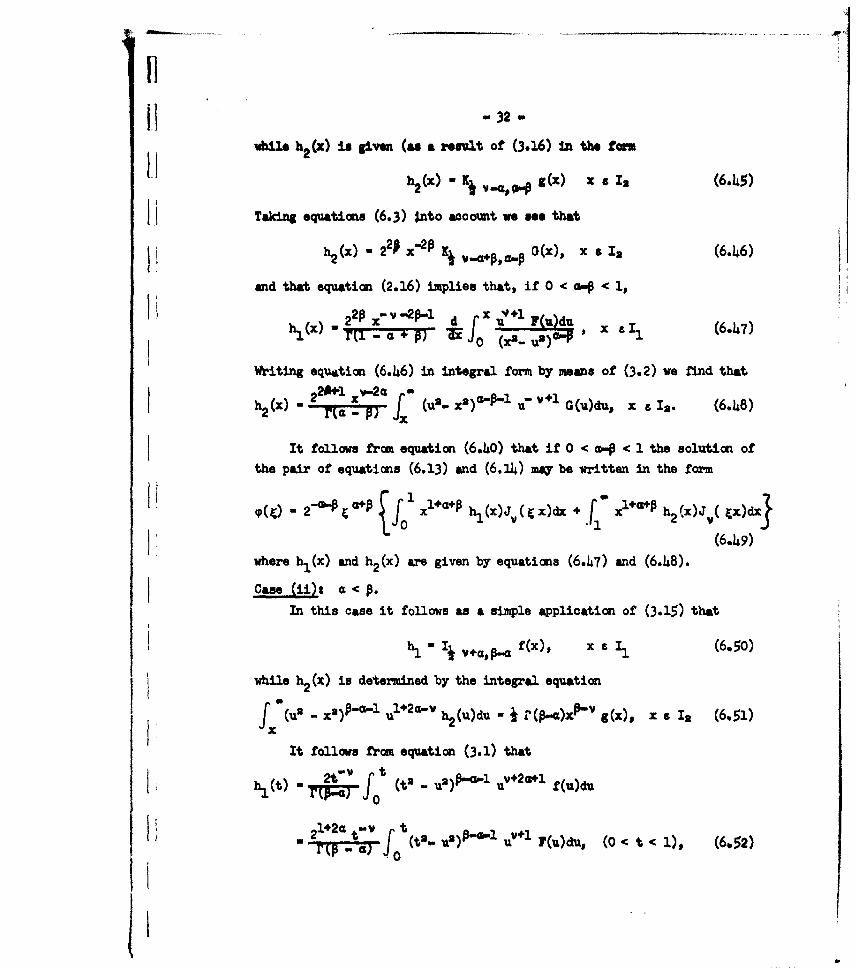
11 II -32.

vhIle h 2 (z) isa given (as a result of (3.16) in the torn

h 2 (x) - Kj , g4 -P9(x) x a( 6-4 5)

Taking equations (6.3) $nto account we see that

(h2 x) - 22P x" • v.-2p,. x), x a 1s (6.46)

and that equation (2.16) implies that, if 0 < ap < 1,

"r2 a÷p ... d ix .u =- P~ F( ' x e, 3 (6.47)

Writing equation (6.46) in integral form by means of (3.2) we find that-221Hl ,•v.2a /"~ v+

h _20x " - (u2- xS)a-P-1 u" v~l G ( u ) du, x . 1.. (6-48)

SIt follows from equation (6.40) that if 0 < *- < 1 the solutim of

the pair of equations (6.13) and (6.14) may be written in the farm

l (6.49)

where hl(x) and h2 (x) are given by equations (6.47) and (6.48).

Case (ii): I <.

In this case it follows as a simple application of (3.15) that

h1 - Ij V~a P f(x), x e I1 (6.50)

while h2 (x) is determined by the integral equation

x a(Us - x 2)P-a--I ul÷2c.' h2Cu)du -" i r'(P.)x•'v g(x), x a 12 (6-51)

It follows from equation (3.1) that

h -. (t)-uk")um. o _ 4yl uv+2,2+1 f(*)2d

142a -V t2__ _-_t" a) u()p'"4 u"+ F(u)dus, (0 < t < 1), (6*52)rI011

Ii -33

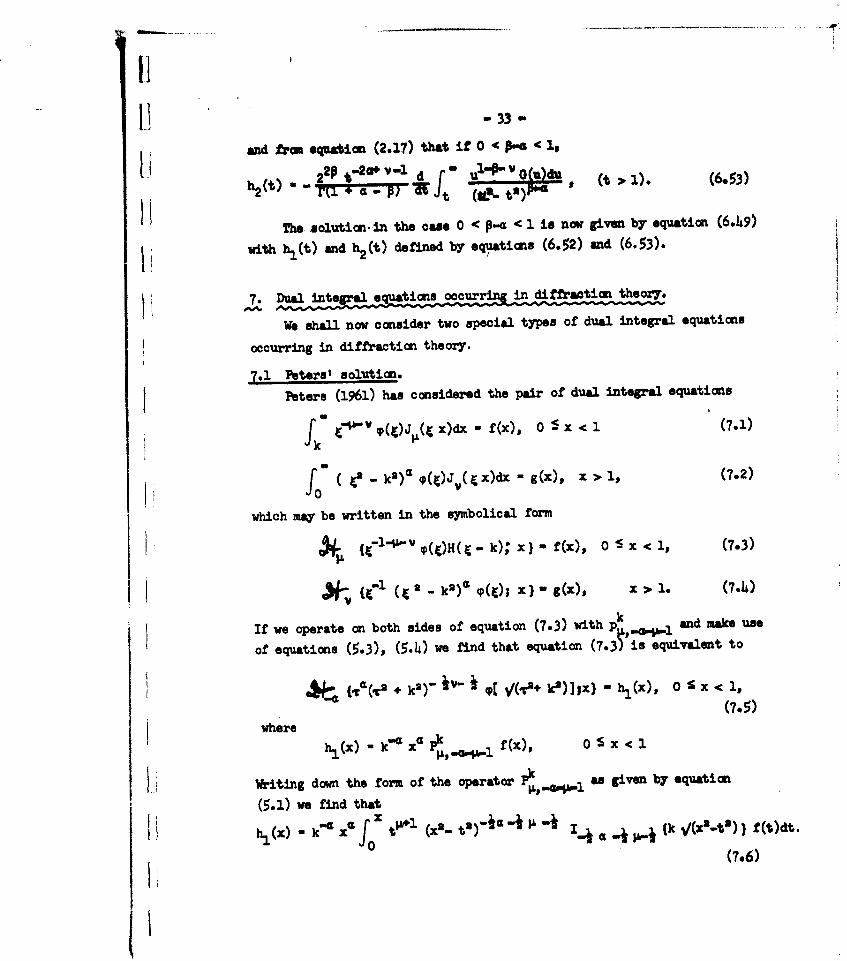
and frmi equation (2.17) that if 0 '-C "1,22P t-20 V-.1 d f a ul'p•'V owdu) ( 1. (6.53)h2(t) " t (IL _ t2•)•

The solution.in the case 0 < P-a < 1 is now given bY equation (6.*49)

with h.(t) and h2 (t) defined by equatims (6.52) ad (6.53).

7 Dul integral equations occurring in diffraction theor7.

We shall now consider two special types of dual integral equations

occurring in diffraction theory.

7.1 Peters' solutin.

Peters (1961) has considered the pair of dual integral equations

fk ei--v p(t)J,(t x)dx - f(x), 0 5 x < 1 (7.1)

0 (�.e- k2)' (pQ)JV(rx)dx - g(x), x ,1, (7.2)

which may be written in the symbolical form

*4 (Cl-11-v (t)H ( t - k); x) f fx), 0 S x -c 1, (7.3)

N-V (1 (pI - k)a (p(t); x) - g(x), x > 1. (7.4)

If we operate on both sides of equation (7.3) with p _ and make use

of equations (5.3), (5.-4) we find that equation (7.3) is equivalent to

( {.rG(gr2 + k2)- iv- i f' k')]Ix) - h.l(x), 0 S < 1,(7.5)

where h 1(x) k_"j- x a 4 p f(x), 0 S x < I

Writing down the form of the operator ,- las given by equation

(5. 1) we find that

)a fO x t')"• "' 4 " 4 (k V(x2-t') ) f(t)dt.hl (x) - k'• x= t (x,. a.•i -i .P •.

(7.6)

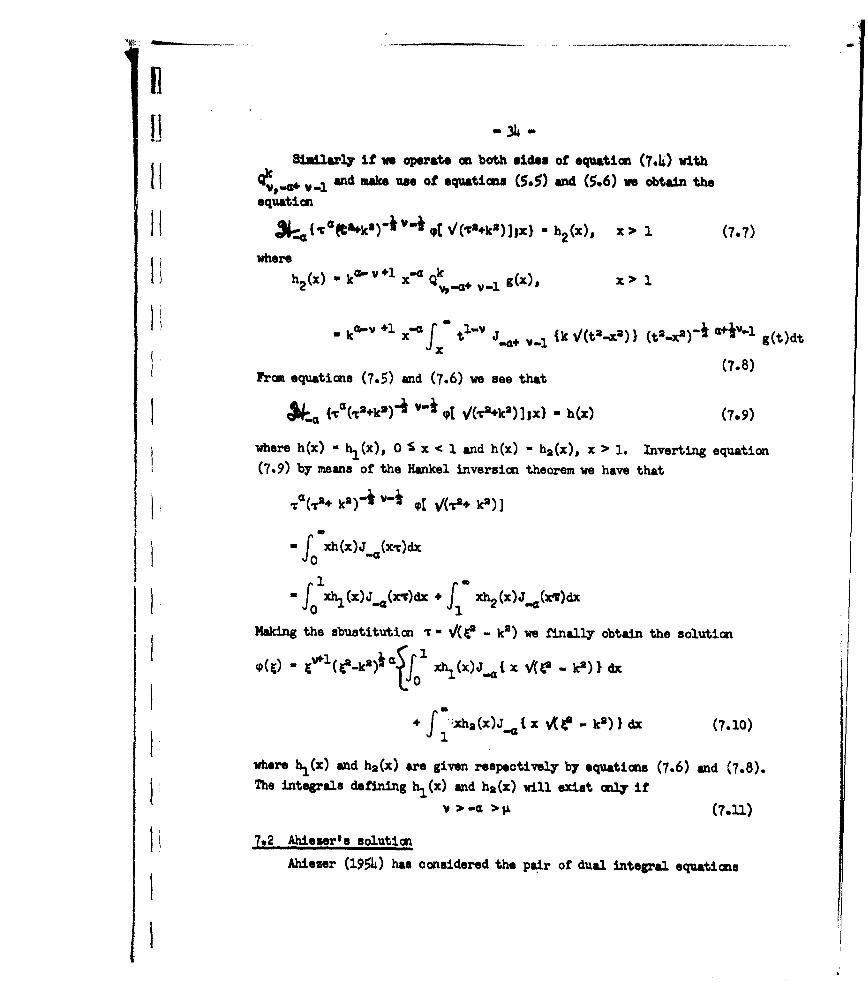
m314

Similarly if we operate an both sides of equation (7.4) with

[1 .,- -1 and make uwe of equatimon (5.5) and (5.6) we obtain theequation

31,.. {¶r a ftka) -*v 4 qPr1/ (104 ) ] x) .h 2(x), (7-7

wherea-v1 ak

h2(x) • k x- Qk VP.+ g(x)e x> 1

k Q-V+1X- f40t -VJ.0+ v-1 (k -v(t2--x2) (t2_2-l O)" ** g~t)dt

From equations (7.5) and (7.6) we see that

-a (•{(•+k') 4 V-1 #I V(,e+k2)],x) - h(x) 79)

where h(x) - hL(x), 0 S x < 1 and h(x) = h2 (x), x> 1. Inverting equation(7.9) by means of the Hankel inversion theorem we have that

.f xhcx)J(x)d

fI Yxi1()J,(*5)dx + xh2(x)J..(xl)dx

Making the sbustitution ¶r = /( -. kI) we finally obtain the solution

o(w-) - l(e-k2)' xh (x)J I x V(t - k2)} dx

+ f a'-xha(x)J a' x -k2) ) dx (7.10)

where h.(x) and h2 (x) are given respectively by equations (7.6) and (7.8).

The integrals defining h.(x) and ha(x) will exist only if

V >-a > $ (7.11)

S7*2 Ahieser's solution

Ahiezer (1954) has considered the pair of dual integral equations

II

1113 -3%

(o(1OJ.(x-)d uf(x), 0 < x < 1 (7.12)

fH (f " - k2)4 ,(C)j 0 (zC)dg - 0, x > 1, (7.13)

with -1 <a 1< . These equations can be writtemi in the symbolic forms

S(4 p(4)H(C - k) x) -f(x), 0<x < 1

If we act cn both sides of the first of these equations with the operator

_ ,and on both sides of the second ome with the operator -1 ando,.ao, -1-amake use of equations (5.3) and (5.5) we find that these equations are

equivalent to the relations

*,_a (Tl÷" ('r + k 2)-1 (pt¢(, + k2) ];x} 0 x- k Po. f(x),

0 < x 1, (7.14)

S¶a( 3 + k p)+p[ V/(t2 + k')];x )" 0, X > 1.

respectively.

Now, since we have the relation

d xl -a (1-a

we see that the second of theme equations is equivalent to the equation

d .xl• . (T8+ . k')' s/(%O + k-) • ] -0

which may be integrated to give• - 1-+11 (.T + ka)'4 f#1 V(.2 + k2)];X} -•XOWI, P .I 7I;

where c is an arbitrary constant. Applying the Henkel inversion theoremto equations (7.14) and (7.15) we obtain the solutio

S.-+( +k2)-* V(%/.2 + k' 2 -0 f, X1 j 1-,(x -w)dx

+ +fo 1 XJo('T)X),. f (x)dx.- (7.16)

Ii

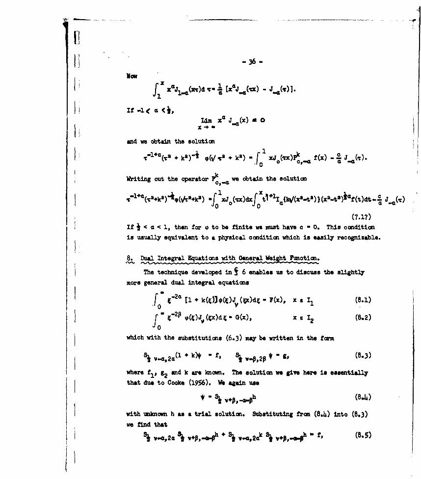
e-36

V If -1 Gif -x

Li xo J,•x W ao1x1

and we obtain the solution

+44- PV,+ 2 i(C~ f (X) j(I '°' k',- 4 ,(• r'. * 3)-. fe xoJCc),. G• -- G . ,

Writing out the operator P we obtain the solution1 x

•.ul÷G(•a~ka ) 4 '(•'+kx) 01 ()dx '•I{/(x'..t )}(x3.t2 )A4f(t)dt-• (

.(7.17)If ac < 1, then for to be finite we must have c - 0. This condition

is usually equivalent to a physical condition which is easily recognizable.

8. Dual Integral Equations with General Weight Functian.

The technique developed in S 6 enables us to discuss the slightly

more general dual integral equations

l El-. [+ k(4)3(P)J (Vc)dg - F(x), x¢ I1 (8.1)o1 V0" a-2p q(t)J, (4x)dh- 0(x), x 9 12 (8.2)

which with the substitutions (6.3) may be written in the flam

Si v-.,,2a(l k>4 - f# v.%.p,2p * - 9P (8.3)

where f1 , g2 and k are known. The solutiom we give here is essentially

that due to Cooke (1956). We again use

* ~ p _G p (8.4)

with unknown h as a trial solutiuon. ststituting from (8.4) into (8.3)

we find that

j v,2, 8* ,+p,.o.Q.Ph + Bj 6%.2 k I* , -,.. ai (8.5)

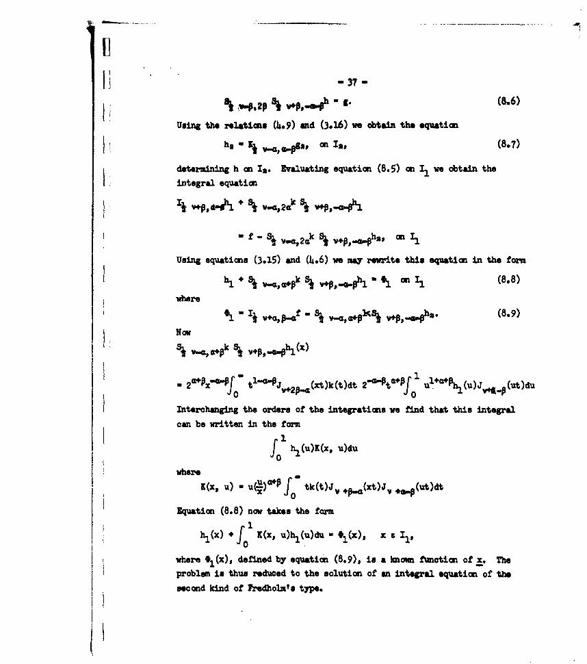
Using the relatlons (•,.9) and (3.16) ws obtain the . quatimt

V he- j 6 , 8 2P on12 (8.7)

deter•i•ing h on In. Evaluating equation (8.5) on 3i we obtain the

integral equation

vIP d~ + %* v-a,2ak %* v~p,w-&%Ol

Using equations (3.15) and (4.6) we may rewrite this equation in the form

hl + j *a,,m.pk *v~p,_phl -11 m 1, (8.8)

where

#1 4 8*p-d V-,+P!. V+"ý (8.9)

Now

SW V-d 8*p % VPP-4-4hl W)

2 , t v2- (xt)k(t)dt 2-0-t"Pfo ulaPluJvCput

Interchanging the orders of the integrations we find that this integral

can be written in the form

fo h1 (u)K(x, u)du

where Kx )-u. +where) U•o• tk(t)J ( +Pa(rt)Jx Te(ut)dt

Equation (8.8) now takes the form

e (x) o n(x,o u)i(n)du -r(x), x t,

where 11(x), defined by equation (8,9),, in a knom flotion of x. Theproblem in thus reduced to the solution of an integral equation of the

second kind of Fredholm's typee

-38-

Table Ipztr

adthe Modified 20ao of Hankel Transforms

i z z .. (3.9)

y~no 'no(3.11)

a - a- (3.16)

j 1 ~(x) - x rx2+a2nl fW(3.21)

K f(x)_ (,)nxl-lj'n x2n-2G42I* I f (x) (.5

S;Is *i(4-5)

s -a8r+~p0KTRO (4-9)

Sr p ýx n Gp(.0Sa(~,p'oGp(-1

I - 39-

-Cu

N. I. AhbeNp, 19 . "On Sam Integral Equations". Dokl. Akad. NaukSSa(n...-)2 333.

i. w. Bubrifto 1938 . "Dual e p qaions". Proc. London Math. Soc.,

G. Doetach, 1937. "Theorie Und Anwendung der Laplace Transformation"(Springer, Berlin).

A. Ardelyip 940O. "On Fractional Integration and its Application to theTheory of Henkel Transforms". Quart. J. Math. Oxford Series,n_2 293.

A. Nrdelyl, 1954. "Tables of Integral Transforms". (McGraw-Hill, New York).

A. Irdelyi and H. Kober, 1940. "Sam Remarks on Henkel Transform". Quart.J. Math., Oxford Ser., 11, 212.

A. Drdelyl and I. N. Sneddon, 0Fractional Integration and Dual IntegralEquations". Canadian ý.. Math.

0. H. Hard and J. E. Littlewood, 1928. "Sam Properties of FractionalIntegrals: I". Math. Zsitschrift, 2L 565.

H. Kober, 1940. "On Fractional Integrals and Derivatives". Quart. J. Math.,Oxford Ser., 0. 193.

H. Kobort 1941a.b Quart. J. Math., Oxford Ser., 1, 78.

H. Kober, t.4b.Trans* Amer. Math. Soc., s , 160.

L L Lore & L. C. Young, 1938. "On Fractional Integration by Parts", Proc.London Math. Soo. (2), ., 1.

N. Lowengrub and I. N. 9neddon, 1962. "The Solution of a Pair of Dual

Integral Squations". Proc. Glasgow Math. Assoc.

B. Noble, 1958. "Certain Dual Integral Equations". Journ. Math Phys., Z128.

A. S. Peters, 1961. "Certain Dual Integral Equations and Soine's Integrals".. N. New York University, Institute of Mathematical Sciences, Rept. 285.

I. N. Moedn, 1962. "A Note on the Relations Between Fourier Transformsand Henkel Transforms". Bull. Pol. Acad. Sci.

3. C. Titcbehrsh, 1937. "Introduction to the Theory of Fourier Integrals".Clarendon Press, Oxford.

0. 1. VWtem,. 1*9. *A Treatise m the Theory of Resel F]•timos. UniversityPreos, Cambridge.

H. eYl, 1917., m g sum Begriff des Differentialquotienten gebrochenerOwdnumg". Vierielu . Naturforech. Gen. Zurich, 62 296.

V. R. &lliam1 , 1962. "The Solution of Certain Dual Integral Equations'. Proc.Edinburgh Math. Soc.

A. Zypmnd, 1959. "Trigonometric Series'. 2nd edition, University Press,Camb~ridge.

II

t

I)

11