UNCLASSIFIED

AD NUMBER

AD823514

NEW LIMITATION CHANGE

TOApproved for public release, distributionunlimited

FROMDistribution authorized to U.S. Gov't.agencies and their contractors; CriticalTechnology; SEP 1967. Other requests shallbe referred to Air Force MaterialsLaboratory, Attn: Metals and CeramicsDivision, MAM, Wright-Patterson AFB, OH45433.

AUTHORITY

AFML ltr dtd 12 Jan 1972

THIS PAGE IS UNCLASSIFIED

AFML-TR-6-25

A BRE UVE FTANFRMTIX TCNO

OFAICATPNL

B. K. DONALDSON

- RBased on Lectures by

Y. K LIN )PROFESSOR, AERONAUTICAL AND ASTRONAUTICAL

ENGINEERING DEPT.

CL UNIVERSITY OF ILLINOISoF

TECHNICAL REPORT AFML-TR-7-285

SEPTEMBER 1967 0

This douetis subject to special export conatrols and each trauwulital 0to foreign oenet rfrinntoalaa emd nywt roaprwoval of the Metals and Ceran-cs Divsin, MAM, Air Forem Materi-C%

als Laboratory, Wright-Patterson Air Force Base, Ohio 45433.

AIR FORCE MATERIALS LABORATORYRESEARCH AND) TECHNOLOGY DIVISION

AIR SYSTEMS COMMAND"WRIGHT-PA" N AIR FORCE BASE, OHIO

NOTICE/

When Government drawings, specifications, or other data are used for any purposeother than in conneotion with a definitely related Government procurement operation,the United States Government thereby incurs no responsibility nor any obligationwhatsoever; and the fact that the Government may have formulated, furnished, or inany way supplied the said drawings, specifications, or other data, is not to be regardedby implication or otherwise as in any manner licensing the holder or any other personor corporation, or conveying any rights or permission to manufacture, use, or sell anypatented invention that may In any way be related thereto.

Copies of this report should not be returned unless return Is required by security

considerations, contractual obligations, or notice on a specific document.

400 - October 1967 - C0455 - 12-248

A BRIEF SURVEY OF TRANSFER MATRIX TECHNIQUESWITH SPECIAL REFERENCE TO THE ANALYSIS

OF AIRCRAFT PANELS

B. K. DONALDSON

Based on Lectures by

Y. K. LIN

This document is subject to special export controls and each transmittalto foreign governments or foreign nationals may be made only with priorapproval of the Metals and Ceramics Division, MAM, Air Force Materi-als Laboratory, Wright-Patterson Air Force Base, Ohio 45433.

FOREORD

This report was prepared by the Strength and Dynamics Branch,

Metals and Ceramics Division, under Project No. 7351, "Metallic

Materials", Task No. 735106, "Behavior of Metals". This research

work was conducted in the Air Force Materials Laboratory, Directorate

of Laboratories, Wright-Patterson Air Force Base, Ohio by

B. K. Donaldson based on lectures by Y. K. Lin.

This work began in June 1966 and was completed in September

1966. Manuscript released by the author in February 1967 for

publication as an AF?'L Technical Report.

This technical report has been reviewed and is approved.

W. J. TRAChief, Strength and Dynamics BranchMetals and Ceramics DivisionAir Force Materials Laboratory

ii

ABSTRACT

This report offers an introduction to the transfer matrixmethod of analyzing the dynamic behavior of common engineeringstructures, followed by an explanation of the application ofthe transfer matrix method to an array of aircraft panelswhich are continuous over supporting stringers. The skin-stringer problem, important to the prediction of fatigue fail-ures, is discussed for rather general conditions. The rect-angular panels may vary in thickness and length while thestringers may vary in cross-sectional shape and size. Thepanels may be flat or curved, and the curved panels may varyin radius of curvature.

This abstract is subject to special export controls and eachtransmittal to foreign governments and foreign nationals may be madeonly with prior approval of the Metals and Ceramics Division, MAM,Air Force Materials Laboratory, Wright-Patterson Air Force Base,Ohio 45433.

iii

TABLE OF CONTENTS

I. Introduction ........................ 1

II. The Myklestad Beam Problem .......... 3

III. The Continuous Beam Problem ......... 15

IV. Response to Forced Vibration ........ 20

V. Flat Stringer-Panel Systems ......... 25

VI. Curved Stringer-Panel Systems ....... 40

VII. Numerical Computations .............. 60

References ........................... 62

iv

ILLUSTRATIONS

Figure Page

1. Myklestad model beam. 4

2. Massless beam segment. 5

3. Forces and moments acting as a discrete mass. 10

4. Example Myklestad beam. 11

5. Bent beam. 13

6. Continuous mass beam. 15

7. Beam of general configuration. 20

8. Segmented beam of general configuration. 22

9. Flat stringer-panel model. 25

10. A typical stiffening stringer of open thin-walledtype (a) cross section; (b) displacement; (c) for-ces and moment transferred to stringer from skin. 33

11. A typical curved panel. 41

12. Force and moment components of the state vectorshown in their positive directions. 46

v

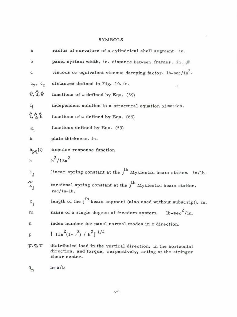
SYMBOLS

a radius of curvature of a cylindrical shell segment. in.

b panel system width, ie. distance between frames. in. .

c viscous or equivalent viscous damping factor. lb-sec/in2

Cy, cz distances defined in Fig. 10. in.

^C, d, 'e functions of w defined by Eqs. (39)

f, independent solution to a structural equation of motion.

^functions of o defined by Eqs. (69)

gh functions defined by Eqs. (59)

h plate thickness, in.

hpq(t) impulse response function

k hg/12a2

k linear spring constant at the jth Myklestad beam station. in/lb.

I-%- thk. torsional spring constant at the j Myklestad beam station.

rad/in-lb.

2. length of the jth beam segment (also used without subscript), in.

m mass of a single degree of freedom system. lb-sec /in.

n index number for panel normal modes in x direction.

p [ 12a2(1-v2) / ha] 1/4

'P, qs • distributed load in the vertical direction, in the horizontaldirection, and torque, respectively, acting at the stringershear center.

q nir a/b

vi

sz distance defined in Fig. 10. in.

t time, an independent variable. sec.

tjk (j,k) element of a transfer matrix.

u deflection of a panel segment parallel to the stringers;positive with the x-axis. in.

v deflection of a panel (segment) or a stringer at the point of

attachment, parallel to the frames; positive, with the corres-ponding coordinate axis. in.

v cV0 deflections parallel to the frames of a stringer cross-sectionat the centroid and shear center, respectively; positive withthe corresponding coordinate axis. in.

w vertical deflection of a panel (segment), or of a stringer at

the point of attachment ; positive down. in.

wc, w vertical deflection of a stringer cross-section at the cen-troid and shear center respectively; positive down. in.

wj vertical deflection of the jth beam segment, positive down.in.

x panel cartesian coordinate parallel to stringers.

x independent cartesian space coordinate for the jth beam segment,

positive to the right. (also used without subscript), in.

y panel cartesian coordinate parallel to frames.

A beam or stringer cross-sectional area. in. 2

[B] conversion matrix defined by Eq. (32) for the flat panel andEq. (66) for curved panels.

C Saint- Venant constant of uniform torsion. in. 4

Cw warping constant of stringer cross-section. in. 6

vii

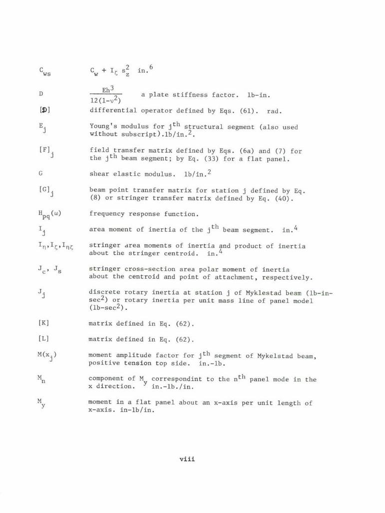
C C+ I( s2 in. 6Cws Cw z

D Eh3 a plate stiffness factor, lb-in.12(l-v 2 )

[1] differential operator defined by Eqs. (61). rad.

E. Young's modulus for jth structural segment (also used3 without subscript).lb/in. 2 .

[F]. field transfer matrix defined by Eqs. (6a) and (7) forthe jth beam segment; by Eq. (33) for a flat panel.

G shear elastic modulus, lb/in. 2

[G]. beam point transfer matrix for station j defined by Eq.(8) or stringer transfer matrix defined by Eq. (40).

H pq(W) frequency response function.

I. area moment of inertia of the jth beam segment. in. 4

IiI•,In stringer area moments of inertia and product of inertiaabout the stringer centroid. in. 4

Jc' is stringer cross-section area polar moment of inertiaabout the centroid and point of attachment, respectively.

J. discrete rotary inertia at station j of Myklestad beam (lb-in-sec 2 ) or rotary inertia per unit mass line of panel model(lb-sec 2 ).

[K] matrix defined in Eq. (62).

[L] matrix defined in Eq. (62).

M(xj) moment amplitude factor for jth segment of Mykelstad beam,positive tension top side. in.-lb.

Mn component of M correspondint to the nth panel mode in they.-x direction. in.-lb./in.

M moment in a flat panel about an x-axis per unit length ofY x-axis. in-lb/in.

viii

M• moment in a curved panel about an x-axis per unit length ofx-axis. in. -lb. /in.

N number of Myklestad massless beam segments (or one lessthan the total number of beam stations.

N tensile force in a curved panel parallel to the frames per unitlength in the x direction. lb/in.

N~x shear force in the x-plane parallel to the frames, per unit

length in the a4 direction. lb/in.

p q an arbitrary force or moment at station q.

[R] . field tramsfer matrix defined by equation (29).

[T] transfer matrix from position indicated by subscript and super-script on right side, to position indicated on left side.

.thV(xj) shear amplitude factor for j segment of Myklestad beam,

positive up on right hand end. lb.

thVn component of V corresponding to the n panel mode in the

x direction. 1. /in.

V Y shear in a flat panel in the z direction on a unit length in thex direction, positive down. lb. /in.

VO shear in a curved panel in the z direction on a unit length inthe x direction, positive down. lb/in.

th

X xj vertical deflection amplitude factor for j segment of a beam,positive down. in.

thy panel normal modal amplitude function of y for n mode. in.

n

{z} beam state vector defined by Eqs. (6) and (7); or a panel statevector defined by Eq. (32) or before Eq. (54).

'ij coefficients to be determined for the functions f.. See Eqs. (60).1

lx

8 ij coefficients to be determined for the functions gi. See Eqs. (60).

Y,6,C structural damping factors. non-dimensional.

Yi' 6 i real and imaginary parts respectively of the characteristicroots of the shell segment equation. See Eqs. (50), i=1,2.rad.

6(t) Dirac delta function - See footnote, page 20.

C damping factor for single degree of freedom system = c/2-r,. rad.

rni quantities defined in Eq. (56). (i=1,2,3).

e. angular width of curved panel segment (See Fig. 11). rad.J

X. panel span width between stringers.J

Pi discrete mass at station j of Mykelstad beam. lb-sec 2 /in.

V Poisson's ratio. rad.

{0} column matrix of biharmonic functions defined by Eqs. (60). rad.

P mass density lb-sec2 /in. 4

a a root of the characteristic equation of the equation of motion --defined by Eq. (19a) for the distributed mass beam, by Eqs. (26)for the flat panel system. rad./in.

angular coordinate of curved panel segment whose correspondingarc is parallel to the frames. rad.

W circular frequency of vibration. A subscript n indicates anatural frequency.

A(M) frequency determinant value as a function of w.O(xj) bending slope amplitude factor for jth segment of Mykelstad

beam = X'(x) rad.

x

Ai constant of integration of a structural equation ofmotion.

{E} state vector defined by Eq. (65).

Tn"'n,"n amplitude functions of p for the deflections u, w, andv respectively. See Eqs. (48).

Q a deflection or bending slope response.P

xi

I. INTRODUCTION

The following presentation is an attempt to clearly outline thetransfer matrix method of analyzing the dynamic behavior of an elasticsystem and, at the same time, to explain a recent extension of thistheory to aircraft type panel-stringer construction[ 1] . For additionalintroductory information the reader is referred to Reference [I] .

The technique of transfer matrices is related to the methods ofdynamic analysis developed by Holzer[ 3] and Myklestad[4l. Likethese previous methods, the transfer matrix method is a calculationof the deflections and internal forces at successive values of a singlespace coordinate (stations) by utilizing a knowledge of the systemintertia, damping, and stiffness properties between stations. Thus,the similarity of these procedures extends to the computation of sys-tem natural frequencies by iterative procedures, to the determinationof normal modes, and to the calculation of deflection and force andmoment type responses in the case of forced vibrations. In other words,the transfer matrix method accomplishes the same types of objectivesin much the same manner as the Holzer and Myklestad methods. Thedifference between these older techniques and the transfer matrixtechnique lies in the advantage of conciseness that results from theuse of matrix algebra by the latter method. This advantage has madepracticable the analysis in detail of complex structures such as singlerows of curved panels supported at varying intervals by not necessarilysymmetrical stringers. The use of matrix algebra does not compro-mise the original advantages of the Holzer-Myklestad style of analysis.For example, the transfer matrix method allows the introduction ofappropriate and separate damping descriptions at each component ofthe structure. Considering the advances that are currently beingmade in damping technology[ 5] , this is no small advantage. On theother hand, the transfer matrix method leads to certain difficulties innumerical computation. These problems and their remedies that haveproven to be effective will be briefly discussed.

To explain the principles of the transfer matrix method a seriesof examples of increasing complexity will be employed. These examplesalso illustrate the scope of this procedure which is presently limited to"a structure undergoing sinusoidal motion(or being in static equilibrium--"a special case), and to a structure being one dimensional in space orwhose mathematical description is reducible to that where the unknownamplitude factor is a function of just one variable. An example of thelatter alternative is a thin plate of rectangular shape which is simplysupported at two opposite edges. In the case of a single frequencyvibration, we could write for the vertical deflection

1

w(x,y,t) = eidt Yn (Y) sin nfx

where y is the space coordinate parallel to the simply supported edges,and Yn(y) describes the variation of w in the y direction. In otherwords, we have reduced a plate problem to a one dimensional problemsusceptible of solution by transfer matrix methods by (justifiably)assuming the form of the deflection with respect to one of the spacecoordinates.

The examples in the order of their discussion are (1) an undampedbeam with discrete masses, (2) an undamped and damped beam with distrib-uted mass properties, (3) the calculation of frequency response functionsfor a beam, (4) a flat panel-stringer row, and (5) a curved panel-stringerrow. The first three examples are for explanatory purposes. The last twoare summaries of recent extensions of transfer matrix methods.

2

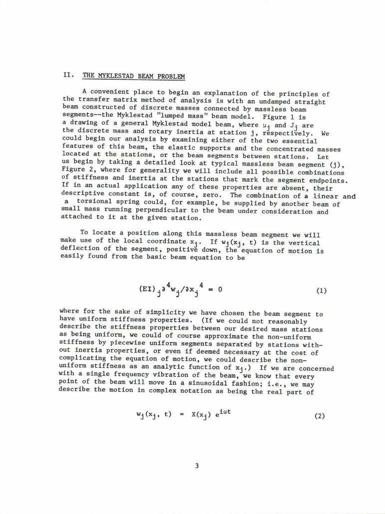
II. THE MYKLESTAD BEAM PROBLEM

A convenient place to begin an explanation of the principles ofthe transfer matrix method of analysis is with an undamped straightbeam constructed of discrete masses connected by massless beamsegments--the Myklestad "lumped mass" beam model. Figure 1 isa drawing of a general Myklestad model beam, where pj and Jj arethe discrete mass and rotary inertia at station J, respectively. Wecould begin our analysis by examining either of the two essentialfeatures of this beam, the elastic supports and the concentrated masseslocated at the stations, or the beam segments between stations. Letus begin by taking a detailed look at typical massless beam segment (j),Figure 2, where for generality we will include all possible combinationsof stiffness and inertia at the stations that mark the segment endpoints.If in an actual application any of these properties are absent, theirdescriptive constant is, of course, zero. The combination of a linear anda torsional spring could, for example, be supplied by another beam ofsmall mass running perpendicular to the beam under consideration andattached to it at the given station.

To locate a position along this massless beam segment we willmake use of the local coordinate xj. If wj(xj, t) is the verticaldeflection of the segment, positive down, the equation of motion iseasily found from the basic beam equation to be

(EI) a4Wj = 0 (1)

where for the sake of simplicity we have chosen the beam segment tohave uniform stiffness properties. (If we could not reasonablydescribe the stiffness properties between our desired mass stationsas being uniform, we could of course approximate the non-uniformstiffness by piecewise uniform segments separated by stations with-out inertia properties, or even if deemed necessary at the cost ofcomplicating the equation of motion, we could describe the non-uniform stiffness as an analytic function of xj.) If we are concernedwith a single frequency vibration of the beam, we know that everypoint of the beam will move in a sinusoidal fashion; i.e., we maydescribe the motion in complex notation as being the real part of

wj(xj, t) = X(xj) eiwt (2)

3

0

-0 -r-

a4i -H-

0

4 -J

U)U)a)

C))U))

41 i

-riq

0))

C'4 0

- - - 4-J C - - C

-~ i') 4-)

04W

r44

00

4-) 4-

0 0)

'H

0 ~~4-/H --

4-

,.I

En

ca

a)

"t-'to-i)

,--tIU

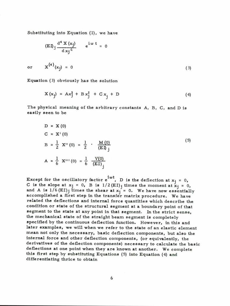
Substituting into Equation (1), we have

(EI)j d 4 X (xj) e t=

or X(4)(xj) = 0 (3)

Equation (3) obviously has the solution

X(xj) = Ax] + Bx 2 + Cxj + D (4)xj j

The physical meaning of the arbitrary constants A, B, C, and D iseasily seen to be

D = X(0)

C X '(0)

1 _1 1 M(00 (5)B 1 ~ X"(O) - 2 "E~2 (EA j

1 X"1(0) V(O)A 6 X( - (EI)j

- iwtExcept for the oscillatory factor e , D is the deflection at xj = 0,C is the slope at xj = 0, B is 1/2(EI)j times the moment atxj = 0,and A is 1/6 (EI)j times the shear at xj = 0. We have now essentiallyaccomplished a first step in the transfer matrix procedure. We haverelated the deflections and internal force quantities which describe thecondition or state of the structural segment at a boundary point of thatsegment to the state at any point in that segment. In the strict sense,the mechanical state of the straight beam segment is completelyspecified by the continuous deflection function. However, in this andlater examples, we will when we refer to the state of an elastic elementmean not only the necessary, basic deflection components, but also theinternal force and other deflection components, (or equivalently, thederivatives of the deflection components) necessary to calculate the basicdeflections at one point when they are known at another. We completethis first step by substituting Equations (5) into Equation (4) anddifferentiating thrice to obtain

6

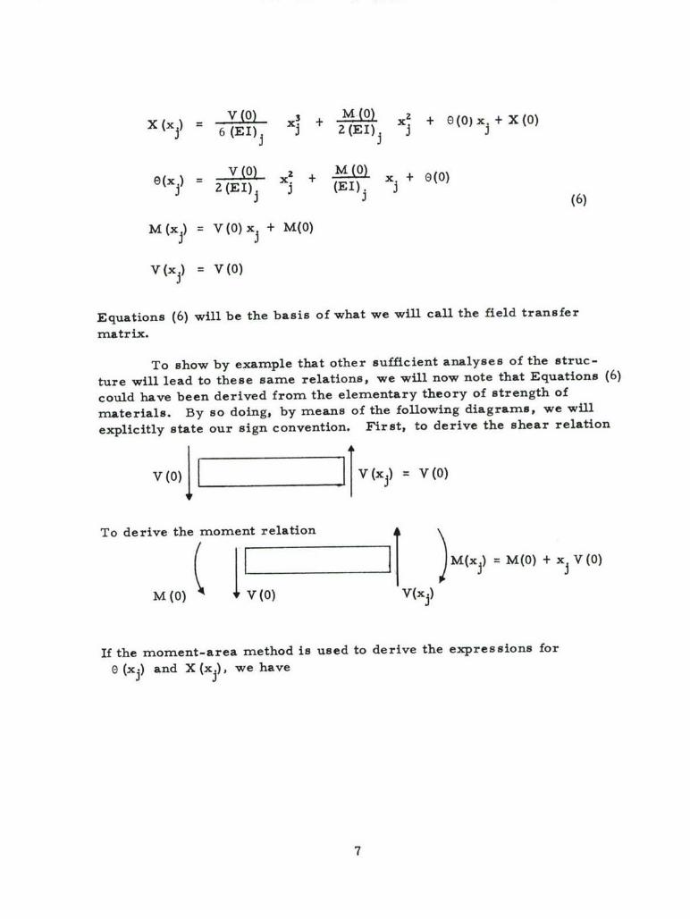
X(x) = V(o) x 3 + M(O) X2 + o(Ox +X(O)

e(xj) = V() 2 + (0)+)(O(EI) j (EI) x + ()(6)

M (x l) = V (o) xj + M(O)

V(x ) = V(o)

Equations (6) will be the basis of what we will call the field transfer

matrix.

To show by example that other sufficient analyses of the struc-

ture will lead to these same relations, we will now note that Equations (6)

could have been derived from the elementary theory of strength of

materials. By so doing, by means of the following diagrams, we will

explicitly state our sign convention. First, to derive the shear relation

V (0) jI IV (xi) = V(0)

To derive the moment relation

M(0) ( IV(O) V(xj) M(xj) = M(O) + x v (o)

If the moment-area method is used to derive the expressions for

0 (xj) and X (xj), we have

7

_______~X V__ _ _ _ j (0)/(EI)

El

Once again

E)(X) E) (0) + M(O)U Xj + v (0) Xi (E I) i (EI) i

X (X) X X(O) + 0 (0) x + M (0)- + v () .

If we now specialize Eqs. (6) by letting Xj = Iiwe may view theresult as a means of carrying over or transferring the mechanicalstate of the beam at the right hand side of station J-1 to the left handside of station j. We may easily arrange this series of transferequations in matrix form as follows

X-%I -1 1 P P -rX rZEI 6EI

00 1El ZEI (6a)M 0 0 1 1 M

V 3 0 0 0 1 V j-1

8

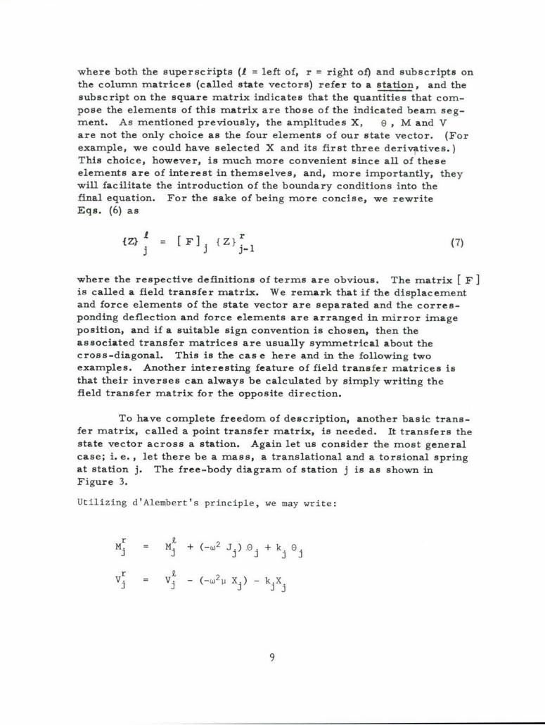
where both the superscripts (I = left of, r = right of) and subscripts onthe column matrices (called state vectors) refer to a station, and thesubscript on the square matrix indicates that the quantities that com-pose the elements of this matrix are those of the indicated beam seg-ment. As mentioned previously, the amplitudes X, 0, M and Vare not the only choice as the four elements of our state vector. (Forexample, we could have selected X and its first three derivatives.)This choice, however, is much more convenient since all of theseelements are of interest in themselves, and, more importantly, theywill facilitate the introduction of the boundary conditions into thefinal equation. For the sake of being more concise, we rewriteEqs. (6) as

z [F] {Z}r (7)zJ j j-1

where the respective definitions of terms are obvious. The matrix [ F]is called a field transfer matrix. We remark that if the displacementand force elements of the state vector are separated and the corres-ponding deflection and force elements are arranged in mirror imageposition, and if a suitable sign convention is chosen, then theassociated transfer matrices are usually symmetrical about thecross-diagonal. This is the cas e here and in the following twoexamples. Another interesting feature of field transfer matrices isthat their inverses can always be calculated by simply writing thefield transfer matrix for the opposite direction.

To have complete freedom of description, another basic trans-fer matrix, called a point transfer matrix, is needed. It transfers thestate vector across a station. Again let us consider the most generalcase; i. e. , let there be a mass, a translational and a torsional springat station j. The free-body diagram of station j is as shown inFigure 3.

Utilizing d'Alembert's principle, we may write:

r kM. = Mj + (_W2 j.) .0 + k* 0.

r

Vj = V. _ (- 2 p X) -k X

9

k .X

_• 2 j. e.

J ]

3 J

_•• xjI'~ X I

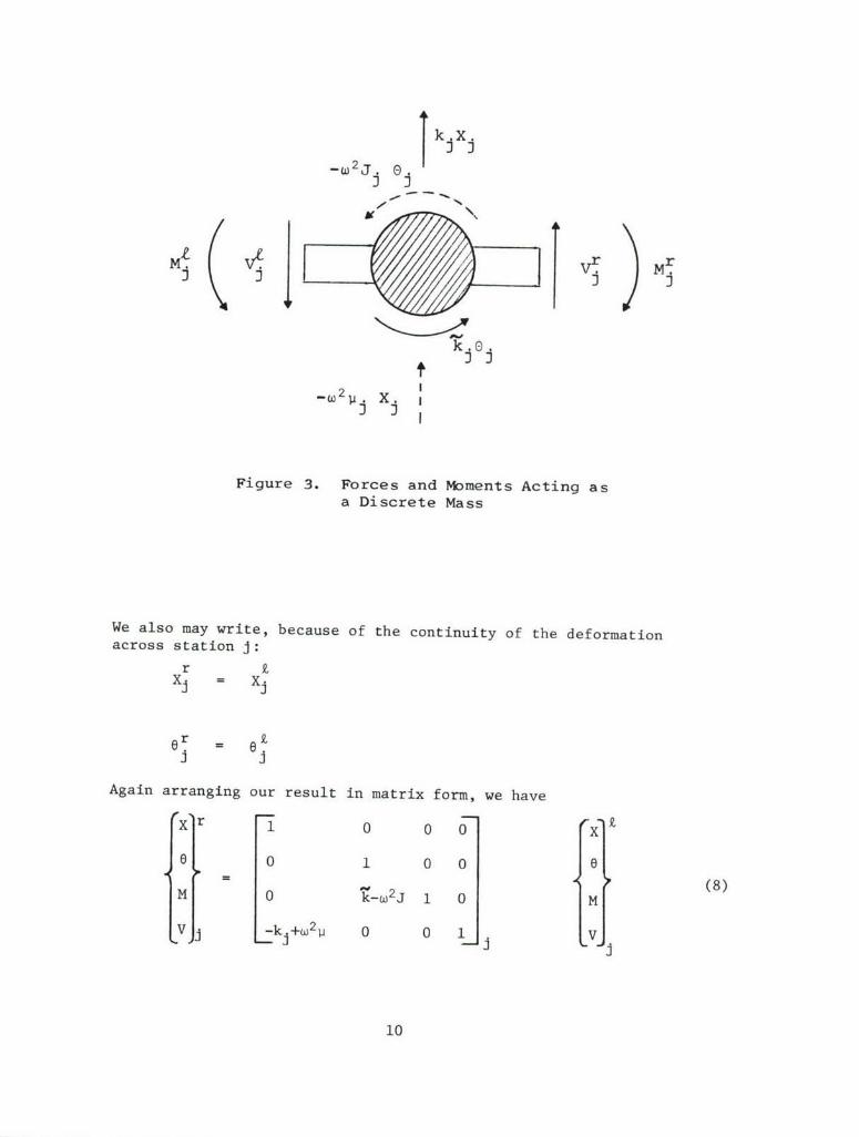
Figure 3. Forces and Moments Acting asa Discrete Mass

We also may write, because of the continuity of the deformationacross station J:

r £x. = x.

r = 2.J J

Again arranging our result in matrix form, we have

Xr 1 0 0 0

0 0 1 0 0 0

(8)M 0 "-o2J 1 0 M

V --k +w2j 0 0 1 j Vfj

10

or

Z}r = [G] {Z}1 (8a)j j J

We are now ready to undertake the analysis of any undampedMyklestad beam possessing any end conditions. To make clear the gen-eral case, we choose the specific beam shown in Figure 4 where anycombination of elastic restraints may be present at the three inter-mediate stations.

0 1 2 3 4

Figure 4. Example Myklestad Beam

Proceeding from left to right, we may by successively applying Eqs. (7)and (8) write

! r{Z 1 = [F] 1 {Z} r

1z 0

{Z}r= [G]l [F] 1 {Z},1 r

{Z1 = [F] [G] "'" [GI [F] {Z} r4 4 3 1 1 0

or more concisely

{Z} I = I r {}r(9:4 4 0 0

We call [ T ] a transfer matrix; i.e., no adjective. Its superscriptsand subscripts indicate the extent of the transfer of the state vector.The boundary conditions of our example are:

at (1, 4) X = E = 0

at (r, 0) X = M = 0

11

(A similar result would ensue for other boundary conditions.) Insert-ing these boundary conditions in the matrix equation (9) we have

,,%It Pt--0 tll t12 t13 t140

o t 2 1 t 2 2 t 2 3 t 2 4 0

M t 3 1 t 3 2 t 3 3 t 3 4 0

V t 4 1 t 4 2 t 4 3 t 4 4 V4 4_ 0 • 0

from which we note that we may extract two linear homogeneous equa-tions, i. e., the submatrix equation

:I tj: t14 I r (10)04 tZ z t2 4 o0 0

The existence of a nontrivial solution to Eq. (10) requires that thedeterminant of the coefficients be equal to zero, Since these coef-ficients are all functions of the free vibration frequency, our equationfor the natural frequencies of the system is then

tl 2 t14 r

= A(w) 0 (11)4 t 2 2 t 0 0

Since A(w) will for this model, be a polynomial in w z of order equalto the number of intertia parameters, both rotary and translational, anumerical rather than an exact solution for w is to be obtained inalmost all cases. Of course, all the roots for w2 are real and positive.Once the natural frequencies are known from equation (11), it is a simplematter to compute the force and deflection mode shapes for this beam.We start with Eq. (10) which tells us

L = - V -- V (12)tl2 tzz

12

If, for example, we normalize (i. e. assign a unit value to) V, we knowall four components of the modal state vector at (r, 0). It is now onlynecessary to use the transfer matrices [G(w n) I and [ F(xj]) to com-pute the modal state vector at any point of continuity on the beam.

The above steps are the basic elements of the transfer matrixapproach. In review, we start at one point of the structure andproceed to an adjacent point using whatever state vector is necessaryto describe plus transfer the mechanical state of the structure. Thetransfer matrices that carry the state vector from one point to anothercan be calculated by solving the overall equation(s) of motion of eachstructural segment. When the proper field and point transfer matricesare determined, a transfer matrix from one boundary to another canbe constructed, and then partitioned to solve for the natural frequencies andmode shapes.

The present analysis could be expanded, for instance, to con-sideration of the vertical vibrations of a cantilevered beam with ahorizontal bend. We could further slightly complicate the matter byplacing the concentrated masses and rotary inertias on rigid extensionsfrom the beam axis. This model might be a suitable model for acantilevered high aspect ratio wing. See Figure 5.

Elastic Axis/

Concentrated

BeamI I

Figure 5. Bent Beam

13

We won't stop to analyze this model, but only comment on those

of its features that are not found in the previous example. First,

simply because of the horizontal bend, a vertical force or bending

moment on the outboard section of the beam will produce a torsional

moment (and deflection) as well as a bending moment on the inboard

section. Therefore we would have to include the local beam twist and

torsional moment in an analysis of this structure. Secondly, even

without the horizontal bend, we would be compelled to consider tor-

sional twist and torsional moment because the vertical accelerationsof the offset concentrated masses would produce inertial torques

about the beam axis. Therefore, our model would properly include

not only the rotary inertias associated with bending slope deflec-

tions, but also the rotary inertias corresponding to torsional de-

flections, and cross products of inertia.

We could start our analysis at the beam tip and work our way

toward the bend just as in the previous example. (The additional equa-

tion of motion for a massless beam segment is: the effective torsional

stiffness times the second derivative of the twisting angle equals zero.

The equations of motion of beam stations can again be derived using

D'Alembert's principle.) At the bend we simply connect the locally

oriented state vectors on each side of the bend by a matrix that resolves

the outboard set of deflections and internal forces into components

referenced to the inboard coordinate system. (Matrices are a rather

efficient way of handling coordinate rotations.)

We are not limited to models where the inertia properties aremade discrete. Let us now investigate how we may apply the transfer

matrix method to a beam with distributed inertia properties.

14

MI. THE CONTINUOUS BEAM PROBLEM

Consider the case of a uniform beam segment of symmetric cross-section and of uniform density between two stations, say j-i and J.

See Figure 6.

X.I JI

S(EI)j, Pj, A.j

j-1j

Figure 6. Continuous Mass Beam

The equation of motion of this segment can be derived from the basic

beam bending equation, It is, for vibrating motion

a4wEI - = - pA i& (13)

where p is the mass density, A the cross-sectional area, and each

dot above a symbol indicates one partial differentiation with respect

to time. We have dropped the subscript j from our various quan-

tities for the sake of simplifying the writing of our equations. If wewish to examine a single frequency sinusoidally varying motion, we

may again describe the vertical deflection as

w(x, t) = X (x) e ibt

Thus our equation of motion reduces to

Eld4X pAwzX

This equation may be rewritten as

d4 X X = o (14)

15

where a = PAW2 (14a)EI

Four independent solutions to the differential equation (14) are exp(ox),exp(-ax), exp(iax), and exp(-icx). Note that these solutions areindependent regardless of which of the four roots of a4 is used, and infact, the same four functions are obtained regardless of which of thefour roots is used. For later convenience we will specify the use ofthe positive real root. Now any four independent linear combinations ofthe above four solutions are also a complete set of solutions. The mostadvantageous set of combinations is

f~x) 1f (x) = 1 (cosh ox + cos o-x)02

f1 (x) = - (cosh Tx - cos ox)1 (15)

f1 (x) = I (sinhox + sin crx)1

f 3 (x) = - (sinhox - sinox)

The advantages of this set of combinations, the reasons for theirselection, are

(1) f 0 and f 2 are real even functions of x

f, and f 3 are real odd functions of x

(2) The index order rotates under differentiation or integration; e. g.

f' (x) = of 3 (x)

f1 '(x) = T fo (x)

f, (x) = rf1 (x)

f3' (x) = afz (x)

-and (3) f 0 (0) = 1; f (0) = 0 for j 4 0.

Then, when we write our solution in the standard form

X(x) = Ao fo (x) + Al f, (x) + A2 f2 (x) + A3 f3 (x) (16)

we can see by virtue of items (2) and (3) above that we obtain the happy

re suit

16

Ao = X(Q)A (0)

SA 1 =X' (0) or A

T2A 7 X"(0) or A (17)

T A3 X"'(0) or A3 3 --0r El

Thereforeo (0)

X(x) = x(o)fo (x) + f- (x)0.

+ ( fz (x) + V f0 (x) (1 6 a)74 )fE I 3EI

So, once again by obtaining a suitable solution to the equation of motionof an elastic element, we have obtained the basic relation for the fieldtransfer matrix of that element. The remaining relations are, ofcourse, obtained by differentiating Eq. (1 6 a)

X' (x) = rX(o) f 3 (x) + E (0) f0 (x)

SM(0) f, (x) + V-0EfI+ 0El (lf 2 (x)

X,'(x) = T. X(0) f2 (x) + cr 0 (0) f3 (x)

+ M (0) f0 (x) + V(0) f (x)E1 (r EI

X"'(x) = a-3 X(0) f1 (x) + (2 E (0) f2 (x)

+ - (0) f 3 (x) + V() fOWx)E1 E1

17

Combining these results for xj = Ij in matrix form, we have

xI fo (1) xf2 (I f 3 rr (TZ E I 1 E0

0 -f3 (1)) f f (M) a-ED 0

T (rEI

(18)

M a-Z EIfz (1) a-EIf 3 (1) f 0 (1) Li M

V T 3 EIf1 (1) a-2 EIf2 (1) a-f3 (1) f 0 (1) V

Note that this field transfer matrix is also cross-symmetrical.

At this point, let us include damping effects as part of ouranalysis. We do so in the realization that for a damped systemsinusoidal motion exists only when the system is subjected to asinusoidal excitation. Structural damping at joints and in elasticsegments can easily be included in the conventional manner in our

equations of motion. At joints, that is at the location of elasticsprings, we introduce structural damping by simply replacingkby k(1 + 16) and k by k (1 + ic) where 6 and E are structuraldamping factors. Similarly, structural damping in an elasticelement is described by replacing EI by EI(1 + iy), where y isanother structural damping factor. Of course, these changes in theequations of motion are carried through in identical form to the pointand field transfer matrices. We may also take into account anequivalent viscous damping by adding another term to our equationsof motion. For example, the equation for an elastic segment becomes

EI(1i+ iy) - + c& + p A;h = 0

with no external excitation on this particular segment. To solve thisequation we again let w = X (x) exp (i w t), and substitute to obtain

d4 X pwz A - icw = 0 (19)77 - EI(l+Iy)

18

We can return to the form of equation (14) by simply redefining a as

4 = pW2 A - icw (19a)EI(l+iy)

Thus, again, the field transfer matrix, Eq. (18) retains the same form.In this case all the quartic roots are complex. As before it is permis-sible to use any one of the four roots as a in the computation since weonly requirethat sinhux, coshox, sinax, and cosax be independent of eachother.

Thus, since the form of the transfer matrices remains unalteredby the presence of damping effects, in our subsequent examples we willtake for granted the presence of the various damping parameters intheir appropriate locations.

As a final comment, before we pass to the topics of forcedvibration and skin-stringer construction, the method of transfer matricescan also be applied to beam grids and frames[ 2 ]. Very briefly, a singlepath through the structure is chosen and by means of the continuity andequilibrium equations of the Joints and the boundary conditions at beamends other than the two that mark the beginning and end of the chosenpath, the structure that lies off the chosen path is represented bypoint transfer matrices on the chosen path.

19

IV. RESPONSE TO FORCED VIBRATION

Before we see how to use transfer matrices to calculate the

response of a structure to forced vibration, let us pause to review

a bit of the basic theory of mechanical vibrations.

The response to a structure under forced vibration, either

deterministic or random, can be described by either of the following

two basic functions [6] :

the impulse response function h (t)pq

the frequency response function Hpq ()

The respective meanings of these two functions are as follows. Let the

structure be at rest at t = 0, and let the excitation be a unit impulse*

applied at station q at time t = 0. Then hpq (t) is the response at

station p. See Figure 7 below. Let the structure be stable (say

positivply damped), and let the excitation be a unit sinusoidally varying

load (e co) applied at station q. Then the stead, state response at

station p is Hpq (M) eiwt.

h(t) or H(w)e i~t I (0) e •i~t

0 01

P qI

Figure 7. Beam of General Configuration

* A unit impulse at time T=t is described mathematically by the

Dirac delta function, 6(t-T). Its definition is, for an arbitraryfunction r(t)

Co t+E

r(t) = 6(). 5(t - T)dT = I F(T). 6(t - T)dT

where e is arbitrarily small. It is sometimes described as a func-tional because it is not a function in the ordinary sense, i.e. while6(t) = 0 for almost all t, it is not specifically defined for t withinthe interval (t- E, t +e), 6 arbitrarily small.

20

An arbitrary forcing function can be considered as a continuoussequence of impulses, i. e. we may write

P (t) = f+° P (")6(t- r)di-q -to q

A response at station p to the forcing function can be described withthe aid of the appropriate impulse response function for the two stations,i.e.

+oo0

(t) =f - P (T) h (t- T)dTp -CXD q pq

On the other hand, if a spectral analysis of the forcing function is per-formed so that

Pq Wt = + 0T; (w) e iWt dw

q -OD q

where 1 • -• +a, -iwtPq() = -f + P (t) e dt-0 q

then the response to the forcing function Pq (t) can be written

(t) f "0 Pq (w)H (w) e dw

p ODpq

Using a few simple steps we can show that

00- icot

H (w) foo h(t) e dtpq -00

h (t) 1 DH (w) eit dwpq pq

That is,outside of the adjustment of a constant factor, these functions areFourier transform pairs.

A simple example of these functions is to be found in the case ofa single degree of freedom system. Here p = q = 1 (omitted), and

21

mwex ( ý nt + iw n _•2 for t>O0n n

h (t) =t

0, for t < 0

and

1m(ciz -Wz + Zirwwn)

n

The technique of transfer matrices can be used to computefrequency response functions. For illustration, consider the non-uniform beam with end conditions sketched below.

SII -

STA STA STA STA0 j , k N

Figure 8. Segmented Beam of General Configuration.

The beam is approximated by a finite sequence of uniform sectionsbetween stations. Any arrangement of interior elastic supports maybe included in the problem. We are interested in obtaining the responseat station k due to a unit sinusoidal force at station J. We may needto be more specific about the response, that is, decide whether theresponse on the left hand side or the right hand side of station k is theresponse to be calculated. For the sake of definiteness, let us decidewe want to know the response on the right hand side.

22

To develop the equations in a natural way, let us again start at

the left end of the beam and proceed to the right. By our previous

work, we can immediately work our way to the left hand side of the

impressed force.

I r r{z} - [T {Z}3 j 0 0

The impressed force is simply introduced by writing

r0{Z} r = r {Z} +

(Recall the factor e is common to all terms of these equations.)

Proceeding from this point, we have

r r r r{Z } = [ T] {Z}k k

so that

{Z} r [ T ]r {Z} + [ T , (20)k k 0o k J

This is our first of two basic equations. In expanded form it is

X r(20ra)(= r[ T ( + [T 0 ( (a)Mk 0 0 k 0V~k (jo 1

where we have inserted the boundary conditions at station 0. In

addition to the elements of the state vector at (r, k), the slope and

shear at (r, o) are unknown. These elemnreits can be eliminated by use

of the boundary conditions at station N in our second basic equation,

which is merely a continuation of the first equation. It is

0 1 [ T ] r 0 +IT] 0 (21)

= N 0 ( 2 0

S( JT(323

Now, from the above two (4 x 1) matrix equations, (20a) and (21), we canextract the following two equations, respectively.

Xrr -t 1 4 r r r r

(tZ 2 tZ 4 + tZ 4

[ t3 2 t34 k t34Vjk J 42 t 4 4 j 0 t44 +

14] r Jr + uf

Then solving the second of these for Jr If

= I_ t l 2 t 4 r tl 4 I 4N t22 t24 o NLt24

and substituting this quantity into the first, we obtain

r r r r rtX t 2 t 1 4 t 2 2t 4

:: : (iI4 iz t]J 1 + (22)

V t4 2 t3 4 4 44Sk k 0 k_0

The left hand side is the set of amplitudes of the response as functionsof the frequency w due to a unit sinusoidal force excitation, which bydefinition are the frequency response functions for these circum-stances. Of course, the frequency response functions for a unitsinusoidal moment can be obtained in an exactly analogous way. Theresult is

"r r r r rx t 2 t1 4 t1111

M0 = t22 tZ 4 TL 2 tj] r)N[ 3 j + t3 (22a)

M t3 2 t3 4 II t~ 2 4 t2 4)t 3vI t4 Z t4 4 k t43. k k k_

Of course, other boundary conditions lead to the selection of otherelements of the transfer matrices.

24

V. FLAT STRINGER-PANEL SYSTEMS

We will discuss two types of stringer-panel systems. We willbegin with flat stringer-panel systems, and when we have determined themethod of solution for these, we will proceed to discuss the moreocmplex case of curved panel systems. A sketch of a typical flat panelarray is shown in Figure 9.

Frame (Simple Support)

Str-nger !_

Frame (Simple Support)

Panel No.

12 j

rFI tL L1 2 j-1 j N

Stringer No.

Figure 9. Flat stringer-panel model

To simplify the presentation of both the flat and curved panelanalyses, we will limit our attention to free, undamped vibrations.The treatment of the cases of damped and forced vibrations, as hasbeen explained, is little different. A simple forced vibration examplewill be given in Section XII.

25

Note that, while in the case of beams we made no restric-tions concerning the boundary conditions, in our flat panel mathe-matical model we specify simple support boundary conditions at theframes. As will be seen, this particular arrangement allows us toreduce this essentially two dimensional problem to a one dimensionalproblem. As pointed out before, once we have a one dimensionalproblem, we may employ the method of transfer matrices. Mostactual construction is not such that the conditions of simple sup-port exist at the frames. However, because the distance betweenstringers is usually one half or less than one half the distancebetween frames, and since fatigue failure can be expected to beginin the panel skin adjacent to the center of a stringer, this modelis quite practical for the study of the important problem of fatiguestresses in actual panel construction. More generally, this sameargument can be extended to claim validity for applying the resultsof this model to construction with different boundary conditions atthe frames if the response of interest is located near the mid-distance line between frames.

The standard plate bending equation of motion for the panelskin is

a4w + 4w 34w h

Dx 4 + 2 ax2 a + -p w (23)

For a discussion of the underlying assumptions and derivation ofEq. (23) see Reference [7], pages 39-1 through 39-3. In this problem,with simple support at the frames, we may obtain a solution in theform

w(x, y, t) = eiwt Yn (Y) sin _ (24)b

where we take advantage of the known modal form in the x-direction.For each n, the function Yn is the amplitude function in the y-directionIt corresponds to X(x) in the beam problem, and this unknown is, ofcourse, only a function of one space coordinate.

Substituting Eq. (24) into Eq. (23), after cancelling exp(iwt)and sin(mrix/b), we obtain for each stringerwise modal number n

26

(4) - +•--\ Y + Yn (n h Yn (.25)Z~~(B'r Yfl+n) ~

We have two unknowns in the one equation, w and Yn" We need

to determine those special values of w (in mathematical terms the

eigenvalues, or in dynamical terms the natural frequencies) for

which we can also determine solutions for Yn up to an arbitrary multi-

plicative constant, (the eigenfunctions, or normal modes of an undamped

system.)

We can write the characteristic roots of Eq. (25) as +o , -ai,

+icz, and -iT 2 where

= _12 (26)

(D/4 1h/4 1/4 2

Since for each n, (D 1nr /h P b) is the smallest natural

frequency of an infinitely long panel row without stringers[ 8] , and

because the addition of stringers and boundary conditions at a finite

distance would increase the stiffness and hence the natural frequen-

cies of such a built-up, finite system, we can conclude that U2 is areal quantity.

Let us now turn to our transfer matrix techniques. We are

here interested in determining the deflection, slope, moment, and

shear in the panel skin along any plane perpendicular to the x-axis.

The deflection and slope, of course, depend upon Yn and Y'n

respectively. Since[71

My +D -- 2-w +

Sa Yw aw

V =+ D a- a-- + a 2

27

we see that we can describe these quantities of interest by employingYn and its first three derivatives. Therefore, as a stepping-stone toour final state vector Lyn Yn' Mn VJ, let us consider the state vectorLYn YA Y" Y'J and discover how it may be transferred across a field,i.e. across a panel.

We already have the first part of the solution to the panel prob-lem in terms of the solutions for the chatacteristic roots of our reducedequation of motion, Eq. (26). These roots, of course, allow us towrite a solution for Yn in terms of (e.g. expodential functions of) wfor each panel. Then, analogous to the continuous beam problem, ournext step is to express the panel solution in a form appropriate to ourstate vector Ln Y' Yn n' . Again we start by expressing our solutionin the form of the sum of four independent functions, i.e.

Yn(y) = Ao fo(y) + Al fl(y) + A2 f 2 (y) + A3 f 3 (y) (27)

so that among other conveniences, Ao = Yn(0)' A1 = Yn'(0), A2 = Yn''(0),and A3 = Yn (0). As in the case of the beam, we by-pass solutions inthe form of exponential functions, and concentrate on combinations ofthe hyperbolic and circular functions. Specifically, these independentsolutions are sinh oly, cosh oly, sin 02y, and cos o2y. The combinationof these that we seek is

fo(y) (22 cosh + 2 cos 2 Y)012 + 022 (2o o2y

1 (yy)1 2 012fl(y) 2 2 (-a sinh oy+ - sn 2y012 + 022 0 sinh 0 2y sin o2 y)

S1 2

(28)f 2 (y) 2 1 (cosh oly - cos o2 y)

01 + 022

f 3 (y) a0 2+1 2 sinhoay sin_2y)1 2 2

(A general procedure by which we can calculate the desired functionalforms of our solution will be illustrated for the more complex case ofa curved panel segment.) The functions fo and f 2 are even while fland f 3 are odd, fs(r)(0) = 0 when r # s, and fs(r) = 1 when r = s,for r, s = 0, , 2, 3. However, because 01 # 02, f'(y) 0 fs+l (y);i.e. the nice index rotating property that was present in the case ofthe beam problem does not exist here. As a result of this, we willrequire more than four functions to construct the transfer matrix for

Y1 Y11 Y2

28

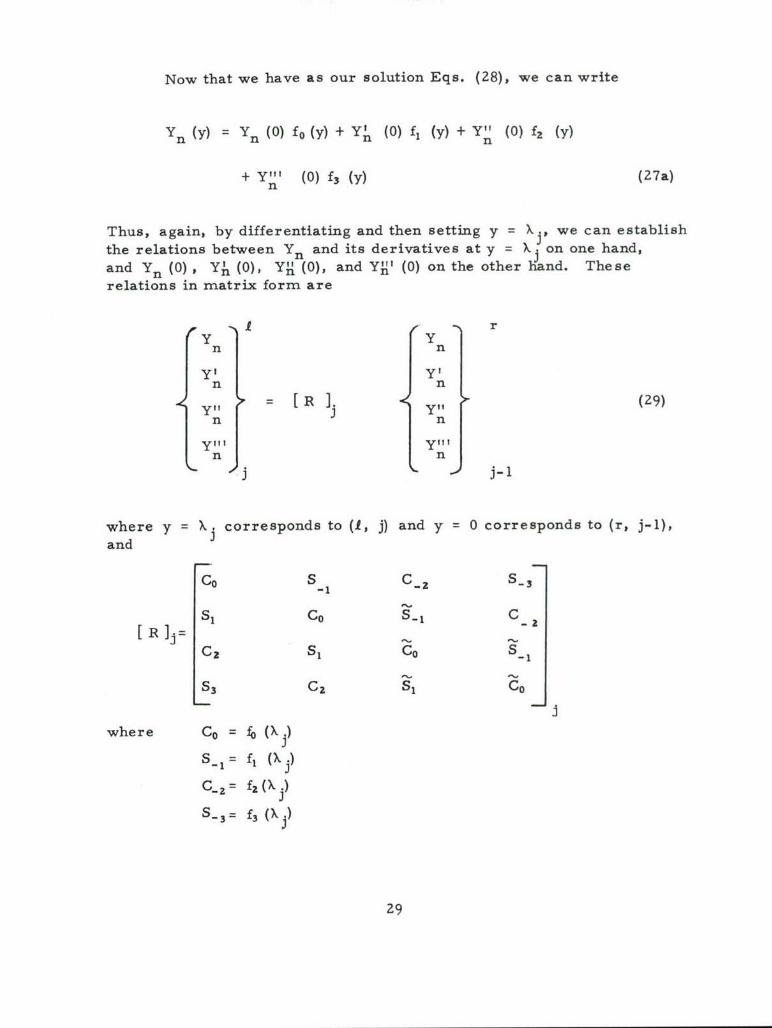
Now that we have as our solution Eqs. (28), we can write

Yn (Y) = Yn (0) fo (Y) + Yn (0) fl (Y) + Yn" (0) f2 (Y)

+ Y"' (0) f 3 (Y) (27a)n

Thus, again, by differentiating and then setting y =k, we can establishthe relations between Yn and its derivatives at y X j on one hand,and Yn (0) , YI (0), Y 4. (0), and YII1 (0) on the other Hand. Theserelations in matrix form are

A ry y

n n

n n

=h e R y =e (29)n n

n n

where y =X. corresponds to (1, j) and y =0 corresponds to (r. j-1),and

CO S C-2 S_3-1 -

S, CO S_1 C[RIj=- ,2-

C2 Si Co S-1

S3 C2 S1 CO

where CO = fo (Xi)

S_1 f, (X%)

Q- 7= f2 (X)

S_3= f3 (Xi)

29

1 2Go + z (0.2 cosh a-, % + 0.T cos (0rz )

0.1i .2 + Cz

Cz = TIz 2 ( (cosh (i r - Cos •02Cr + -( i

S-1= TI, + Cz ((r, sinh cri X. + 0.r sin a- 2)3 3

SI z z (0.2 sinh 01 X- T2 sin vz X.)S, I 3

U1 +3.rSi = + . (0.1~ sinh 0.i X. - 0.3 sin 0.2 Xj)

S3= 3. +.0zZXj

S2 (0.2 sinh 0. , X + 0.z sin Xr )S 3 = 0 i Z+0. G 0i1z .2

At this point we will convert the state vector yn Yn' Yni YI'Jto one which will represent the variations in moment and shear in they direction. We do this by expressing the moment and smax in thesame form as the vertical deflection, i.e.

i (•tM = e Mn (Y) sin nl__x

y b

(30)i6)t

V = e Vn (y) sin n.Txy -b

From Eqs. (27) and (30), by means of the orthogonality properties of thesine function, we can obtain

M (y) = D [Y" -v Y ]n n bn

(31)

V (y) = D [Y"' - (2-- v)(-rJ Y]n n b n

This immediately leads to the matrix form

30

y Yn n

y, Y(n n

{Z} = M =[ B]jy, (32)

V Y "'t

n n

where the conversion matrix and its inverse in detail are

1 0 0 0

O 1 0 0[B]. =

J -Dv(r) 0 D 0

o(Z-V)(RI) D 0 Do10 0 b

1 0 0 0

[B] 0 2 1 0 0=w 0. 1 0

7)• z D

o (z-v)In~F) o0b Dj

Now we are in a position to write

SI rYn Yn

n n

n n

Mn - F] Mn (33)

V Vn n J-n

31

where [F]. = [B]j[R]j [B]: is, of course, the field matrixwhich trans/ers the state vector LYn Yn Mn VnJ across a panel.The matrix [ F I is symmetrical about its cross-diagonal, and[F(bn) 1 = [ F (-bn)].

Now that we can leap panels as we wish, we turn to our lasthurdle, the crossing of stringers. To find the point transfer matrixwhich transfers a state vector across a stringer, we must take acloser look at the stringer. The stringer does not interfere withthe continuity of the deflections and slopes in the skin on either sideof the line of attachment between the stringer and skin. Thus, verysimply,

Yn (r, j) = Yn (1, J)

Y' (r, j) = Yn (A, j)n

However, the stringer, because of its elastic and inertial properties,does produce what we will consider to be an abrupt change in themoment and shear in the skin at the line of attachment. To determinethe form of the change in the shear and moment components of thestate vector we will make use of an existing theory which deals with thebending and torsion of a general thin-walled member of open cross-section. This theory is the result of a number of distinguishedengineers, a few of which are: Timoshenko (in 1908); Wagner (in 1929);Goodier (in 1941); and Argyris (in the early 1950's).

The basic deflection equations of the stringer are

EIw (4) + EI v (4) =-

S(4) (4)EIy Vo + El71 wo = (x) (34)

EC 4( 4) - GC 1" = (x)w

where I , I , and I are the centroidal moments of inertia and pro-duct moment of inertia; G is the shear modulus of elasticity; the sub-script o refers the deflections w and v to the shear center ; C is thewarping constant of the stringer cross section with respect to thew shearcenter ; C is the Saint-Venant constant of uniform torsion; F and [

32

z

z

•> -•

4J

) N0

•I-I -w

Wuo

Q4~

1 0

r r4E-4

-0 0

4.4

0 0) N-,--I

o to p

U 0u4 rO

4-) NU) ý (L)

o~0 r)~~.5-0- N4

44 -'-4-1 4J 0.-r- U. 4-)

a)r-4WN $

>1 00WD

%20U)>1 r.

U) NN

E 0)

33

are the distributed loads at the shear center along the stringer in thez and y directions respectively; F is the distributed torque about theshear center; and primes indicate differentiation with respect to x.The first two of equations (34) can be derived by simply (a) super-imposing the strains of a stringer cross-section due to curvaturesin the two perpendicular planes (plane sections assumed to remainplane); (b) integrating the corresponding stresses to obtain the valuesof the moments in terms of the deflections; and (c) differentiating toobtain the distributed loads. The derivation of the third of Eqs. (34)can be found in Reference [7] , section 36. 8.

The distributed forces and the distributed torque about the shearcenter are a result of the acceleration of the stringer, and (reversingour original point of view) the differences between the forces andmoments in the skin on opposite sides of the point of attachment S.Specific ally

T (W V r + V ) -p A

S(x) = (N - N ) -PA (35(x)= (Mr-M 1 ) - (r NI )s - p cz

4ýz cz

+ pAiw c - J Wc y c

where N• is the amplitude of circumferential tension per unit length;p is the stringer mass density; A is the stringer cross sectionalarea; Jc is the stringer area polar moment of inertia about the cen-troid C; c C ., and s are distances illustrated in Figure 10, andthe subscript c on the deflections refers them to the centroid C.

Our basic equations are expressed in terms of the deflectionsat the stringer shear center 0 and the stringer centroid C. Ourpurpose is, however, to express ourselves in terms of the y-coordinatecontinuous deflections of the panel skin. This can be accomplished bynoting that the deflections of the stringer and those of the skin are thesame at the point of attachment S. As can be seen from Figure 10,the deflections of the stringer at point S (no subscript) are geometricallyrelated to those at the centroid and shear center as follows

34

w = w - s (1-cos wo

V = VO - sz ký( 6V=VO ~z 4 ' (36)

wc =wo + c y

V = V - C LC 0 Z

Substituting these relations into our equations of motion (34) and (35), and

combining and rearranging them, we obtain

Mr _ MI = ECws 4( 4 ) _ GC 4" + EI sz v(4)+ EI 8zW(4)

+ P 3" - pA(c s ) V + pAc y

Vr V- = _EI w 4 ) - EI v(4) EIs z (4))

-pAW - pAc 4"y

N~r - N~ = El•v4 + EI w~ + EI• sz(4

z z+ pA*V + pA (c z- sZ)

where C = C + I s 2 is the warping constant of the stringercross-secwion wAh respect to S as the center of twist, and Js = Jc +

A c 2 + A (cz - sz) 2 is the area polar moment of inertia of the

stringer cross-section with respect to S.

We now recognize that the flat panel system undergoes negligible

lateral motion, i. e. mathematically v = 0. This is in keeping with the

underlying assumptions of our equation of skin motion, Eq. (23). That

is, Eq. (23) is a bending theory equation in which bending of the plateproduces no horizontal motion of points in the plate middle plane. (On

the other hand a bending theory of curved panels will obviously have to

include lateral deflections.) So, substituting v = 0 and 3w = 4 into

Eqs. (37) we obtain

35

Mr - Mk = ECws a5w - GC ý3w

ax 4y ax2ay

+ EI s + PI 3w + PA c aw

x4 z 4 s ayat 2 Y 3t 2

(38)aW• El S 5wVr _ V =-EIn 4"- EIn s 5

a x4 z ax2

a y

PA 22w - PA Cy a3wat2 8y 32t

We conclude the derivation of the point transfer matrix by substitutingthe expressions for w, M, and V, Eqs. (24) and (31), into Eqs. (38) toarrive at

(Mn)r _ (Mn)£ = [ECws (n-)4 + GC(") 2 _w2 pi ]Y'n

+ [EITJ Sz(n)4 -w 2 pAcy]Y

= Yn + c Y'n (39)

(Vn)r - (Vn)' = -[EI (nL) 4 - w2pA]y

- [EI Sz - W2 pA c y]Yn

36

-y - dy'n n

AWe note that the quantities , d, and e are functions of the naturalfrequency. Thus, in conclusion, we can write

{z}' = [G]Iz {z.40

where

[G] : 1 0 0 0

0 1 0 0

a 0

-e -d 0 1S• j

and the subscript j associated with [GI indicates that the elements of thepoint transfer matrix are computed fvom the physical data of the jth

stringer.

The only exceptions to the cross-symmetry of the stringer transfermatrix are the elements d and -d. These exceptions are a result of thestringer cross-section being unsymmetrical; ie. d=O if the section issymmetrical, and when the direction of transfer of the state vector isreversed causing a far-side eccentricity to become a near-side eccen-tricity, d becomes -d.

We now can proceed to calculate the natural frequencies and modesof the entire panel array. Let [TI, with proper subscripts and super-scripts, denote the general transfer matrix relating the state vectors atany two stations on a panel system. For example

z[T]. = [F]k [G]k_ [F]k_ [G] [F]

k jk -1 -1J+1 J5+1

and

rk[T] = [G]k [F]k [G]k-1 ... [F]j+1 [G]j

37

For the purposes of discussion, let us assume that the two extremeends of the panel system are supported by stringers. In this case we

write

{Z}r r [TI P { (41)N N 0 0

where the state vectors are for the free edges just outside the lines of

attachment of the end stringers. Hence in both state vectors the

moment and shear are zero; ie.

{ j ,r {Z£Y 9r

N n 0n

"0 0

o 0N 0

Thus the following two by one matrix equation can be extracted from

equation (41).

(:3• KE::1 :t]• fYn (42)

For this equation to have a non-trivial solution, we must have the fre-

quency determinant equation

r£

t31 t32

= A(w) = 0 (43)

t-41 t42 j

N 30

Fo tiseqatontohae nn-riia sluio, e us hveth38e

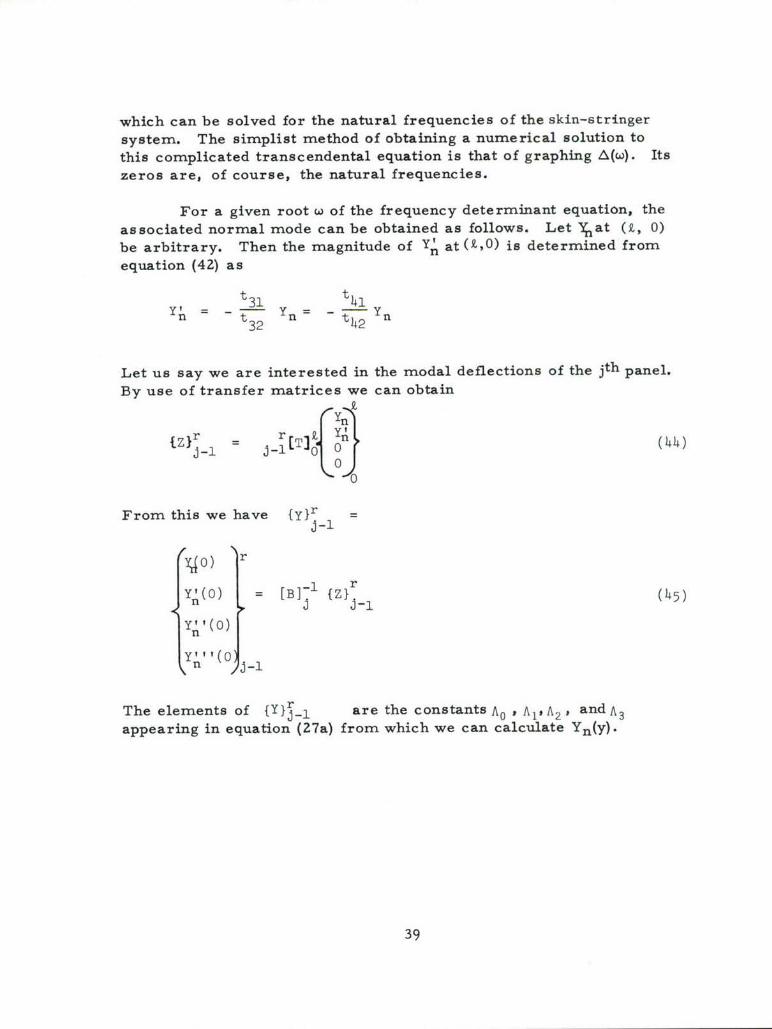
which can be solved for the natural frequencies of the skin-stringer

system. The simplist method of obtaining a numerical solution tothis complicated transcendental equation is that of graphing A(W). Its

zeros are, of course, the natural frequencies.

For a given root w of the frequency determinant equation, theassociated normal mode can be obtained as follows. Let Ynat (X, 0)be arbitrary. Then the magnitude of Y' at (Z,O) is determined fromequation (42) as

t 3 1 t41Yn _Yn - -- YnYn t732t2

Let us say we are interested in the modal deflections of the jth panel.

By use of transfer matrices we can obtain

tZrr r[Z•.I= _[T]' onl (44)

i-ig)(0

From this we have {y}r =

J-1

Y O) r

Y [B-{z}Z (45)

n* C

Yn' (0)

The elements of {y r}J are the constants A0 ,A A2 , andA3

appearing in equation (27a) from which we can calculate Yn(Y)"

39

VI. CURVED STRINGER-PANEL SYSTEMS

The analysis for curved panels is more involved that that forflat panels. It is possible to approach the problem by means of adistributed mass mathematical model, but to reduce the complexity ofthe problem we will lump the distributed panel mass along discrete"mass lines" running parallel to the supporting stringers. The mass

lines will be numbered ... , j-l, j, j+l, .... .The corresponding masses

per unit length of mass line are designated ... , o *j-l'5 , lj j+l"'and the rotationalmoments of inertia per unit length of mass line are• '' Jj-1, J j, Jj+l, ... . The line masses are connected by massless

segments of thin cylindrical shells. This discrete approximation of acurved panel is depicted in Figure 11.

The usefulness of this model is as before dependent upon beingable to consider the panels as simply supported at the frames, i.e. alongthe curved edges. When this ability exists the problem is reducible toone of one dimension, and the same general procedure as carried out inour previous problems will yield a solution.

We will first concern ourselves with developing the field transfermatrix, the matrix which will carry us across the massless shell seg-ments between mass lines. We will base our development of the fieldtransfer matrix on Donnell's shell theory, an approximate theory whichis obtained by eliminating those terms of the more exact theory which areof minor importance to the case at hand. For ar 1 .unloaded and masslesscylindrical shell element, the Donnell equations L 7 J are

2 a2u 9Wa~a - + 1 (1-,) 22u + I a(l+-v) -2v - 03X2 2 Wq2 2 aXa4 DX

1 32u 32 i a)_2 v - w-a(i+v) 2-- + -- + -- a 2 (1l_ ) = w 0 (146)

2 axaý 42 2 3X2 3e

3u 3v I'_t 3'w ___ _4w

va 'u + 'v - w - k a4 +2a 2 a4w + = 0aX4 aX 2 yý 2 Del

where

40

IU

I oI V

Figure 11. A Typical Curved Panel

41

a = the radius of curvature of the segment (note that

this quantity may change from segment to segment)

k = h 2 /12a 2

v = Poisson's ratio

4 = angular coordinate of the shell segment(a4 corresponds to y of the flat panel)

These are two second order and one fourth order partial differentialequations in three unknowns, the displacements u, v, and w. They canbe combined into the following single equation of the eighth order inone unknown.

a 8 kV 8 w + a4(l-V2 ) 94w 0 (47)3x4

where V2 = a2 + 32 and V8 =+ - _V8 = (V )

SX 2 a 2 42

With simple support conditions at the frames, the solutions for the caseof a single frequency oscillation can be written as

u = eiwt Tn(O)cos' n'x

b

v = eiWt Tn(4)sin nx(48

b

42

Substituting the above expression for w into equation (47), we find that

Cn(€) must satisfy the following ordinary differential equation.

(8) - 4q 2 (6) + 6q (4 ) 4_ 6 nn n n % n u n

q+ (qn p4)n 0 (49)

= n•___a = 4 12a2(1-where =Ln b and p - h 2_(I-v 2)

The eight characteristic roots of this equation can be written as

Pcn +

or, to better suit our purposes, in real and imaginary component form

as

+ (Y1 - 61) and

* (Y2 ±6 it 2 )

The values of these components work out to be

Y, = /jý(qn2 + 12 qnp + p2 )1/4 cos(i arc tan PY/7 qn + P

2 + /2 qp + p2) sin(! arc tan ) (50)6,~~~ =%qnqý2r + P

Y2 - q 1 cos[ arc tan pl(vr%- p)]

/h 162 = VO(q.2 - qnp + p 2 )1/4 sin[- arc tan p/(/2 qn -p)]2 n2 nP)

and, in all cases the principal value of the arctangents are to be used.

When the characteristic roots are expressed in terms of their real and

imaginary components, we can say that Eq. (49) is satisfied by any of

the following eight beharmonic functions

43

coshy 1 "* cos6 16, sinhy " sin 61,

coshY24) cos6 24, sinhy 24) sin 62ý,

sinhy 1 • cos61 , coshy 14 sin 6 1,

sinhy24) cos6 2 ¢, coshY24) sin 62Y.

The eight solutions we will use will be linear combinations of the above

solutions so as to facilitate the construction of the field transfer matrix.

We will write our desired solution in the form

7S(4) = X Ai f( (51)

i=O

and, so as to have even subscripts of f imply even functions of €, we

further write for i=O, 2, 4, and 6

f. = a"c.shyl± c0s6 1 ) + a i 2 sinhy1 ) sin 61

+ a i3coshY24 CS624 + ai4 sinh¥2ý sin 62(52)

and to have odd subscripts of f imply odd functions of t, for i=l, 3, 5 and7

fi = aiisinh YI cos 614 + ai2 cosh y1 ) sin 61€ +

(53)ai3 sinhY24 cos 624) + ai4 cosh Y24 sin 624

Before we can construct a field transfer matrix, we must agree on

a suitable state vector. The eight quantities necessary to specify the state

of the cylindrical shell segment are

n , n' ai , (M )n (V )n9 (N n' and (N4)x)nnTn n)n'n4-n' 4n'

These eight quantities in the order given will constitute our statevector. The meaning of the last four quantities is to be seen fromthe following relations[ 7 ]. The second part of these relations arepart of Donnell's theory of cylindrical shells.

M4 = eiwt (M 4)nsin nx£ = D( . 2W +• V x2)

44

S eit(V sin n =x . D [ 1 a 3 w ___ a ____a 0cx2

N = ewt (N )nsin n! x = Eh 1 av wa + -n i-V2 (a a + x

and

N = eiwt (Nx)n sin nx (54)

= Eh a! . _u_ + 3_vv

2(1+v) (a 0 ax

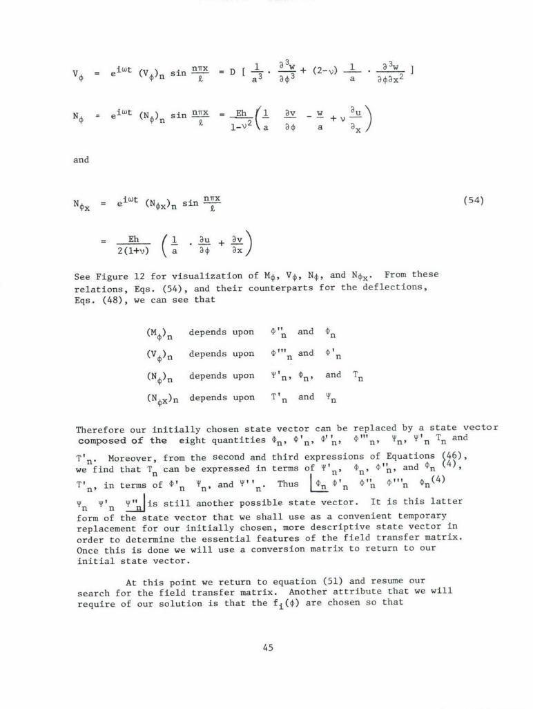
See Figure 12 for visualization of Mý, Vý, Ný, and N~x. From these

relations, Eqs. (54), and their counterparts for the deflections,

Eqs. (48), we can see that

(M ) depends upon 4'" and (D

c n nfn

(V p)n depends upon D'i"ln and 'n

(N ,)n depends upon 'ni, Pn, and Tn

(N~x)n depends upon T'n and Tn

Therefore our initially chosen state vector can be replaced by a state vector

composed of the eight quantities (n, ('Dn' cr', n '"n, nPn Tin Tn and

T'n. Moreover, from the second and third expressions of Equations (46),

we find that Tn can be expressed in terms of T'n, 'n' 'D'n' and Dn (4),

T' in terms of Ofn Tn, and Ti Thus L DIn ("n (Dil (ngnn, n'JP n n n D

n •' 2Jis still another possible state vector. It is this latter

form of the state vector that we shall use as a convenient temporary

replacement for our initially chosen, more descriptive state vector in

order to determine the essential features of the field transfer matrix.

Once this is done we will use a conversion matrix to return to our

initial state vector.

At this point we return to equation (51) and resume our

search for the field transfer matrix. Another attribute that we will

require of our solution is that the fi(ý) are chosen so that

45

'-4

r-I

r-4

c E

.o

H 0

ý4-

,I \ o

4-1

Z/ \ 4-o

4-4

41 0

-0-

19

co -0-Ha3)

ý4-

Z r44

C4J

1-4

Q)-f-4

N

416

A0 = IDn(O) AI = V'n(O)

A2 = ("(O) A3 = 'Pn(O)

A4 = n(4)(0) A5 = n(O)

A6 = T'n(0) AT7 = 'n(0)

One further consideration before we fully develop our solution: the

solution for 'n is not independent of O. From the second and third

equations of (46) we may obtain

T" n + vqn 2 tyn = 711lp In + 1n2 (Dfitn + r'3 n(5)

(56)

where v 11 = 1 + I+2 k qnn4

i-V

n2 = -2 ( 142 ) k qn21-V

1+2 kT3= 1-v

Now let us define7

n(O)= I Ai gi(¢) (57)

i=0

Then

Ai(g"i + vn 2 gi) =i Ai(n f'i + n2 f'i + n3 fi

Since this is true for any set of A., Eq. (56) becomes a relation be-

tween the functions gi(O) and fi(€4 for any particular i; i.e.

g" i + -qn 2gi = nl f'i + n2fi + n3 fi(58)

We note that gi(O) is an odd function if fi(f) is an even function, and

vice versa. A property of the f i functions, which we will use again

later, is their essential permanence of form under differentiation ex-

47

cept that the odd functions become even, and vice versa. Thus a solutionfor gi(*) may be written in the form

gi (¢) = ýil sinh y14 cos 61ý + 4i2 cosh Y1¢ sin 61ý

(59a)+ ýi3 sinh Y2ý cos 62ý + Bi4 cosh Y24 sin 621

for i=O, 2, 4, 6;and

gi(9 ) = BiI cosh Yl4 cos 61ý + ýi2 sinh y1¢ sin 61ý

+ ýi3 cosh Y24 cos 62ý + 3i4 sinh Y2P sin 62ý

for i=1, 3, 5, and 7.It will be convenient to collect these various definitions of f and giinto matrix form as:for i=O, 2, 4, or 6.

fi() a il i2 Ui 3 ai4j {

(60a)

S= L'i i2 6i3 B41 IE0

for i=l, 3,5, or 7

f iiý = Lai i2 ti 3 i4] I fE.

(60b)

gi() = Lk1 ki2 ýi3 ýi4j {Ce}

where

{Ee} = cosh y1i cos 61ý

sinh yl¢ sin 61ý

cosh "2ý cos 624

sinh -Y2ý sin 62ý

4S

0 = sinh ylý cos 61ý

cosh y1¢ sin 61i

sinh Y2ý cos 624I

cosh Y2' sin 62ý

To obtain our desired solutions for In and Yn we have to evaluate four

constants for each of eight fi functions and each of eight gi functions

or a total of sixty-four constants. We begin by returning to our differ-

ential relation between Pn and Tn in order to relate the a coefficients

to the a coefficients, and thereby reduce immediately the problem to that

of evaluating thirty-two coefficients.

As a step preliminary to shaping the relation between the a and B

coefficients, we want an economical means of describing differentiation

When properly organized, straight forward differentiation yields

d

for i=even, and

d fi(o) = Lail ai2 ai3 aiJ4 ] [D] {fe} (61b)

for i= odd, where

[D) = -61 0 061 ¥i 0 0

0 0 Y2 -6 2

10 0 6 2 Y2

Of course, the similar situation that exists for gi(ý) can easily be deduced

from the above. Therefore differentiation of either fi(ý) or giko) is

equivalent to the application of the matrix of transformation [D] to the

opposite column matrix of biharmonic functions; that is, for example,

differentiation of f i with i even, means replacing {ce} with[D] {&0}.

Now we are ready to relate the 6 coefficients to the a coefficients

by means of Eq. (58). Direct application of the differential operator

y~elds

22

L i_] ( [D) + vn2 []

t~J (nl [D] + n2 [D] n3L )

49

or

Lai] iK] = Laj.J[L]

Lail = ai[L][K]-l (62)

where [I] is the identity matrix, and the definitions of [K] and [L]are clear. Let the coefficients for g'(O) be Kil, K12 , K13 , and K14 ,and those for (9) be Til, Ti2, Ti 3 , and Ti 4 . Then

LKiJ = LaiJ [D] [L] [KI-

LTJ = [ij (D] CLI [K]-1

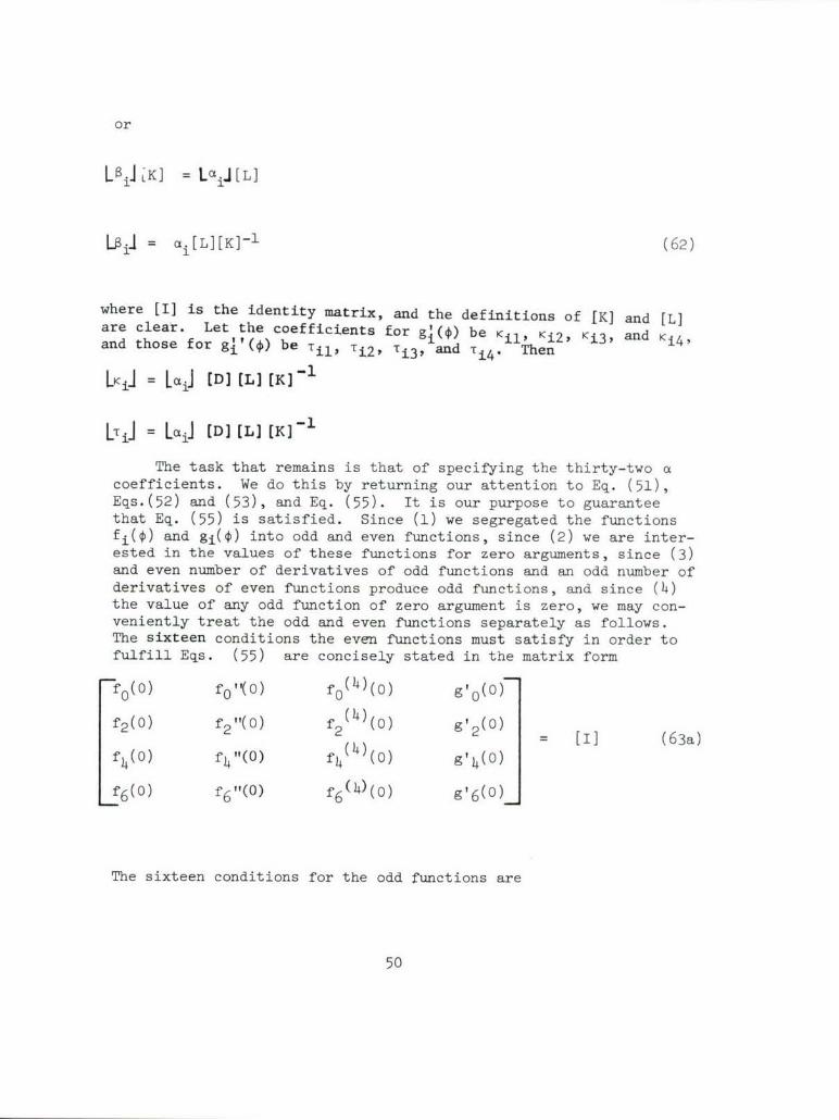
The task that remains is that of specifying the thirty-two acoefficients. We do this by returning our attention to Eq. (51),Eqs.(52) and (53), and Eq. (55). It is our purpose to guaranteethat Eq. (55) is satisfied. Since (1) we segregated the functionsfi(ý) and gi(O) into odd and even functions, since (2) we are inter-ested in the values of these functions for zero arguments, since (3)and even number of derivatives of odd functions and an odd number ofderivatives of even functions produce odd functions, and since (4)the value of any odd function of zero argument is zero, we may con-veniently treat the odd and even functions separately as follows.The sixteen conditions the even functions must satisfy in order tofulfill Eqs. (55) are concisely stated in the matrix form

f0(°) fo '(o) fo(4)(0) g10 (o)

f 2 (0) f 2 "(O) f2( ( 0 ) g' 2 (0) (63a)

f 4 (0) f4"(0) f 4 (4)(0) g' 4 (0)

f6(0) f 6"(0) f6 (4)(o) g'6(0)_

The sixteen conditions for the odd functions are

50

- 1 l(O) f.,11(o) gl(o) g 11l(O

f33(0) f'" 3(0) g33(0) = [I] (63b)

f,5(0) ff' 5(0) g5 (O) g"5 (0)

_fl7(0) fi '7(0) g7 (0) g" 7 (0)

One advantage of treating the even and odd functions separately is that

it reduces the size of the above matrix statements. This is a total of

thirty-two conditions for the thirty-two a coefficients. Let us look at

how these statements in terms of the f 1 (4) and g1 (4) functions may be

conveniently rephrased in terms of the a coefficients. Again considering

the even functions as examples, fo0 (0) = 1 means

Ol 02 03 {o} 1

fo"(O)= 0 means

Lao] [J2 = 0

f0(4)(O) = 0 means

L ot j 1

g'0 (0) = 0 means

LaoJ [j)][LJ(K]_ 0

If we repeat this analysis for the remaining twelve expressions, and

combine our results, they are

a01 a 0 2 aO0 3 a0h1

a2 1 a2 2 a 2 3 a24[IQ] : [II] (64)

a41 a 4 2 a 4 3

a4 4

a 6 1 a6 2 a 6 3 a 6 4

51

where [Q] has as its columns

[)] 2 , [Z]4f and [3)] [L] [KK-111 111

O o 0 0

Hence, for the even functions

[A] = [Q]-' (64a)

and for the odd functions

[A] = [U]-l (64b)

where [U] has as its columns

11 1 1 1

0 0 0 01] , [D]3 [L][K]I , and [0] 2 [L][K]-l

o 0 0 0

At this point we have determined all the functions f.(p) and gi(4) in

7Pn = y Ai f (4 ) (51)

i=0

7Tn(ý) y Ai gi (M) (57)

i=0

and we did this so that Eqs. (55) are satisfied. Hence the state vector

5n n n 2n

52

can be determined at any value of the argument 4 from its value at

€ = 0. That is, in particular we now have the transfer matrix by

which to obtain {E} at 6 = 0..J

[= R] {,}rj j-1

where the elements of [R]j are given by

rkZ = L °i 1 i2 ci 3 3i4j [D] k-l{(j)}

for Z = i+1, k = 1, 2, 3, 4, and 5

and

rk = Lail ai 2 1i3 ei4J [Dl k-6 [L] [K]-1 {(ej)}

for £ = i+1, k = 6, 7, and 8

and where

{Me(e)} = {(e()} for £+k = even

{M(oj)} = {o (0 )} for £+k = odd

The {E} vector is not suitable for the incorporation of boundry con-

ditions, nor does it conveniently mesh with our analysis of stringers.Therefore we will now convert LEJto LZ - n n nl' (M)n(V )n(N~x)

t.~ a n 4 (MW ON4,In\4,The first component of our mixed displacement and force type

state vector can be expressed in terms of the components of V J by

referring to the thkrd of Eqs. (46). From this we find that

Tn(4,) = [1 ' - (1+kq4) (p + 2kq 2 v"n - k(n()]vq n nn n nn

The second, third, and fourth elements of LZJ present no difficulty.

Referring to Eqs. (54), we have

Me = D ( 1 32w + 'V 32wa2 D--2 -X5

53

So,

a 2

Similarly

VO = a 2W [a -- + (2-v)- 32~ ~* cf~ 2 ~ax 2

and

(vC)n=D [¢,,, _ (2-v)q ,n 2 4]a3

Similarly

No Eh 3v - w+ vau

1Nv•2 a 3ý a 3x

so

(N¢) = E (TI -( - vqh T)n a(l_•2) n n nn

- D (q4,D 2- ¢,,n + P(4))

Similarly a 3

= Eh 1 au + av2(---l+9 a - x

so

(N~x) Eh (Tv +q Tn 2a(l+v) n n n

It follows from the second of Donnell's equations, Eqs. (46) that

Tv' = 2 l T-v 2n (14v)q n n l+v n (1+v)q

Therefore

(Ncx) a Eh (q T-n +vqn n qa(1+V) q q

n n

54

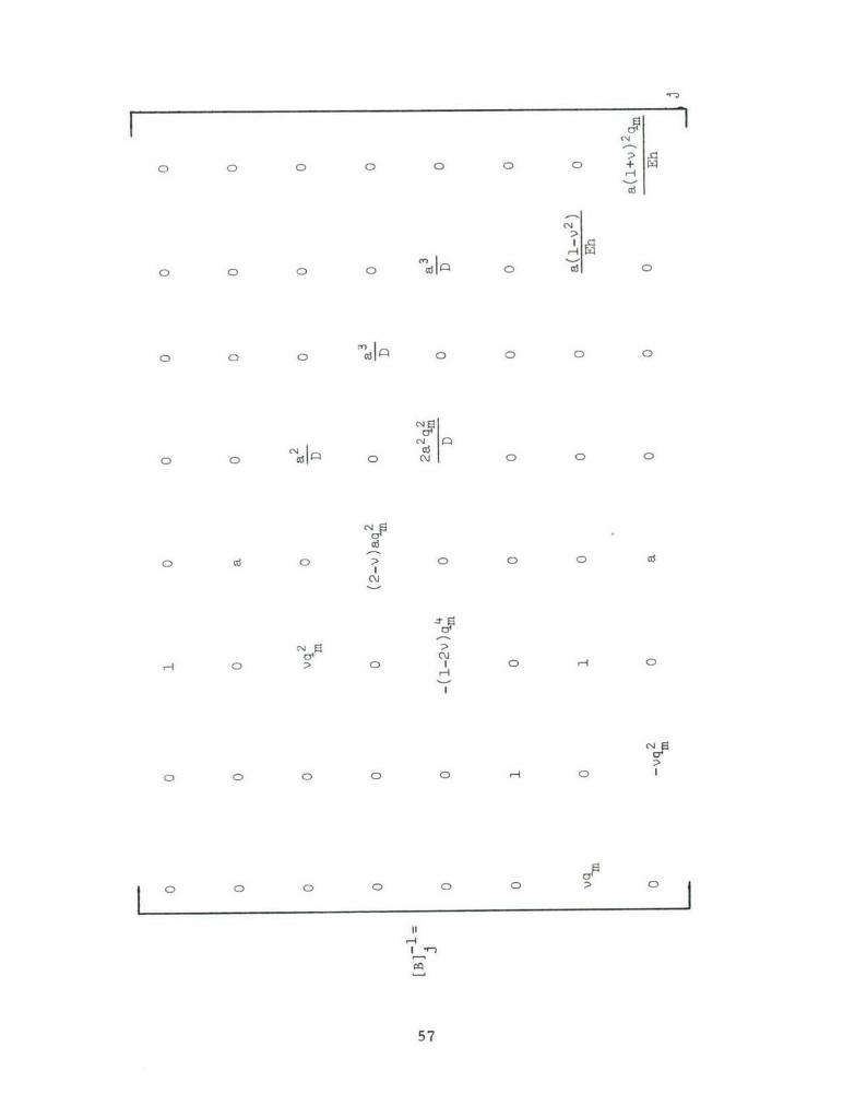
Now we can set up our conversion matrix so that

{Z} = [B]j {I} (66)

where the subscript j is associated with [B] indicates that this matrix

is to be computed from the physical constants of the jth shell segment.

The details of the matrix [ BI j can be found on the following two pages.

The {Z} vectors at the two opposite edges of the jth shell segment can

now be related by writing

[B R [B];1 jZ}j_£ -1i J-{Zlj = [h1j [R]j 1 {~r

S[F] {z}r (67)

This completes our development of the necessary field transfer

matrix, and we now turn our attention to the point transfer matrix

mecessary to account for the effects produced by a stringer and a

mass line. Eqs. (37) are our starting point for the case of a stringer.

If we insert the series expansions for the deflections, monent, shear,

and tensile force into these equations, we can write the result for a

stringer as

(M)r(Me)£'n ^ -- dn~~f

r £-

(M _( = c 1V€ + d 4) + f Yn

nfn a n n n

(Vý)rn -(V )£n = en - d al n -g T n(8

(N )r (N )' Y + 1 0' + 0Sn v n a n n

where the quantities S , d, and e are detailed in Eqs. (39), and

55

0 H0 0 0 0 Q ~

0 0 0 0 0 0 0

oH0 0 0D 0 0 H

Cýlj0 0 0 0: 0CjD)

++

CD CD 0D A 0 0 0D

C~Cd

J -1C'4 ('4r

CM0 0D 01' 0 I6 0

56'

o 0 0 0 0 0 0C

0 0 0 0 0 0

S 0 0 0 0 0 0

Nr-i

I

0 0 0 0 0 -i 0 0

o ciio 0 2 0 0 0•c

H 0 CD C0 CD 0 H0

I5

57

S= sz (nT)4 1 pA(cz - sz)W2

= El r(n, ) (69)

EI (--)- pAW2

The corresponding contributions of a panel skin mass line located atthe same station are-Jw2 ,+pw 2 , and _-w 2 respectively. Thus we maycompose a general point transfer matrix as

1 0 0 0 0 0 0 0

0 1 0 0 0 0 0 0

0 0 1 0 0 0 0 0

0 0 0 1 0 0 0 0

[G] J= 0 f a e-JW2 1 0 0 0

o _-+pW2 - 0 o 1 0 0

o 1_p2 g' 0 0 1 0

0 0 0 0 0 0 0 1

Of course• if no stringer exists at station J, we merely setc= d = e = f = g = h = 0. On the other hand, if there is no panelmass line, Pj = J= 0.

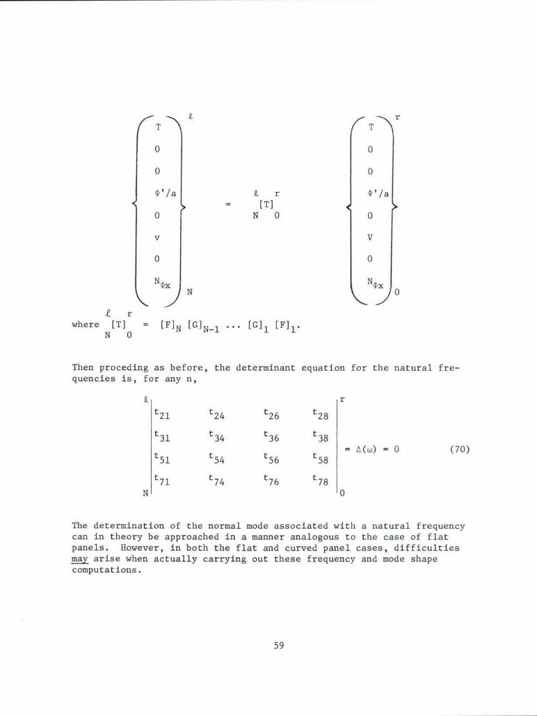
Now that we have described the basic transfer matrices [F] and [G],we can relate the state vectors at any two locations in the panelsystem. We determine the natural frequencies as before by relatingthe state vectors at the two ends of the panel row. For example, ifboth ends of the panel row are simply supported (i.e. T n= n = (M)= (NO)n = 0), these two vectors and the connection between them are,for any value of n

58

T T r

0 0

0 0

'la r/a r= [T]

o N 0 0

v V

o 0

N 0N

L rwhere [T] = [FIN [G]N-1 ... [G] 1 [F] 1 .

N 0

Then proceding as before, the determinant equation for the natural fre-

quencies is, for any n,

rt 21 t 24 t 26 t 28

t 3 1 t34 t36 t38

54= A(w) 58o (70)t 51 t 54 t 56 t 58 AM =0()

t 7 1 t74 t76 t78

N 0

The determination of the normal mode associated with a natural frequencycan in theory be approached in a manner analogous to the case of flatpanels. However, in both the flat and curved panel cases, difficultiesmay arise when actually carrying out these frequency and mode shapecomputations.

59

VII. NUMERICAL COMPUTATIONS

Two types of difficulties can arise when carrying out the numericalsolution of any of the frequency determinant equations. Reference [2],section 7.1 is a good and sufficient explanation of these difficulties.The first of these difficulties is the loss of significant figures when thefrequency determinant is reduced in an ordinary manner. This case isexemplified by Eq. 7-3 of Reference [2]. The second difficulty ariseswhen the elastic supports are very stiff in comparison with the remainderof the structure. The error introduced is explained by Eq. 7-h. In sec-tions 7-2 and 7-3 there are presented two methods of avoiding theseobstacles. The first method, the Delta Matrix method, is limited in thesize of the frequency determinant to which it can be applied. It is notdifficult to apply successfully to a four by four frequency determinant,such as that of a flat panel system, and by dint of much programming,it can also be applied to an eight by eight frequency determinant. Alarger determinant would probably be beyond the capabilities of mostpresent day digital computors. In section 7-h a trial and errorscheme is explained. A short summary of this method is available inReference [1], section IV.

Even when a direct graphical solution of the frequency determi-nant equation is no problem, there is a possibility that the values ofA(w) may pass through zero very abruptlyf9J. Thus, while it is easy tomake a very good estimate of w per se, it is very difficult to obtainnear zero values of A(w) for tRe purpose of computing the mode shapes.As a result, if many transfer matrices are necessary to describe thestructure, the error in the initial state vector will grow to the pointwhere the final state vector is not even approximately representative ofthe given boundry condition at that end. A means of circumventing thiserror accumulation is that of adopting a forced vibration point of view.To begin, sinusoidal shear forces (or moments) of frequencies just oneither side of the natural frequency of interest are applied in turnto the structure, and the respective states of the structure are calcu-lated. If it is found, as would be expected, that the computed statescorresponding to the two such frequencies are very nearly the same, then itmay be concluded that both states are dominated by the same mode--the modecorresponding to the bracketed natural frequency. Therefore it is reason-able to call the averages of the deflection components of these states themode shapes of that nearby natural frequency.

The following example will illustrate the features of the forcedvibration procedure of calculating modal states. Let us apply a sinusoidalshear loading of a unit amplitude at station s of a curved panel withsimple support end conditions. By combining our successive transfermatrix equations we arrive at

6o

0

0

0

IZ}k = k[T ]r Z}r + '[T ]r 0N N 0 0 N s 4 0

10

0 .0

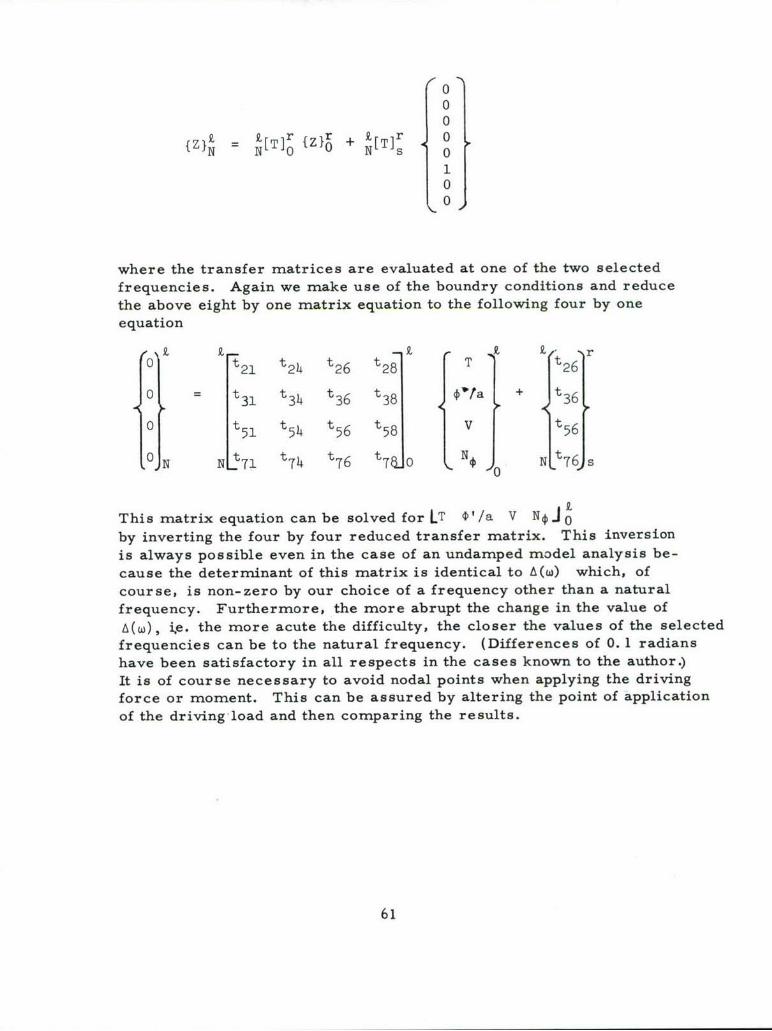
where the transfer matrices are evaluated at one of the two selectedfrequencies. Again we make use of the boundry conditions and reducethe above eight by one matrix equation to the following four by oneequation

0 t2l t24 t26 t28 T t 26

I Z k -- k I I Z - r

0 t 31 t 34 t36 t38 ipta + t 36

0 t 51 t54 t 56 t 58 V t 56

0 JIN Ntt7ý t74 t76 t7UO N N. t 76, s

This matrix equation can be solved for LT 4ý Va V Ný 0

by inverting the four by four reduced transfer matrix. This inversion

is always possible even in the case of an undamped model analysis be-cause the determinant of this matrix is identical to AM which, of

course, is non-zero by our choice of a frequency other than a natural

frequency. Furthermore, the more abrupt the change in the value of

A(w), te. the more acute the difficulty, the closer the values of the selected

frequencies can be to the natural frequency. (Differences of 0. 1 radians

have been satisfactory in all respects in the cases known to the author.)

It is of course necessary to avoid nodal points when applying the driving

force or moment. This can be assured by altering the point of application

of the driving-load and then comparing the results.

61

References

1. Y. K. Lin, et al,"Free Vibration of Continuous Skin-Stringer Panels with Non-Uniform Stringer Spacing and Panel Thickness", AFML-TR-64-347,Part I, February 1965.

2. E. C. Pestel and F. A. Leckie,"Matrix Methods in Elastomechanics", McGraw-Hill, 1963.

3. H. Holzer,"Die Berechnung Der Drehschwingungen", Springer-Verlag,

Berlin, 1921.4. N. 0. Mykelstad,

"A New Method of Calculating Natural Modes of Uncoupled BendingVibration of Airplane Wings and Other Types of Beams," J. Aero.Sci., April, 1944, p. 153.

5. D. I. G. Jones, J. P. Henderson and G. H. Bruns,"Use of Tuned Viscoelastic Dampers for Reduction of Vibrationin Aerospace Structures" Proceedings of the Thirteenth Air ForceScience and Engineering Symposium, 1967.

6. Y. K. Lin,"Probabalistic Theory of Structural Dynamics", McGraw-Hill, 1967.

7. W. Flugge,"Handbook of Engineering Mechanics", McGraw-Hill, 1962.

8. Y. K. Lin,"Free Vibration of Continuous Skin-Stringer Panels", Journal ofApplied Mechanics, Dec. 1960.

9. T. J. McDaniel and B. K. Donaldson,"Free Vibration of Continuous Skin-Stringer Panels with Non-Uniform Stringer Spacing and Panel Thickness". AFML-TR-64-347,Part II.

62

T A ! -,C-T FTRlnSecurity Classification

DOCUMENT CONTROL DATA - R&D(Security classlfication of title, body of abstract and indexing annotation atuat be entered when the overall report is claasstied)

1. ORIGINATING ACTIVITY (Corporate author) 12a. REPORT SECURITY C LASSIFICATION

Air Force Materials Laboratory,I UnclassifiedResearch and Technology Division, 2 GROUPWright-Patterson Air Force Base, Ohio

3. REPORT TITLE

A BRIEF SURVEY OF TRANSFER MALTRIX TECHNIQUES WITH SPECIALREFERENCE TO THE ANALYSIS OF AIRCRAFT PANELS

4. DESCRIPTIVE NOTES (Type of report and inclusive dates)

Technical Report - June 1966 to September 1966S. AUTHOR(S) (Lost name, first name, initial)

Donaldson B.K.

G. REPORT DATE 7a. TOTAL NO. OF PAGES 7b. NO. OF REFS

September 1967 74 9S.. CONTRACT OR GRANT NO. 90. ORIGINATOR'S REPORT NUMBER(S)

b, PROJECT NO.

7351 AFML-TR-67- 285

C. 9b. OTHER REPORT NO(S) (Any otherntumbers that may be atsigned

Task No. 735106thsrpVd.

10. AVAIL ABILITY/LIMITATION NOTICESThis document is subject to special export controlsand each transmittal to foreign governments and foreign nationals may be madeonly with prior approval of the Metals and Ceramics Division, M&M, Air ForceMaterials Laboratory, Wright-Patterson Air Force Base, Ohio 45433.fi. SUPPLEMENTARY NOTES 12. SPONSORING MILITARY ACTIVITY

Strength and Dynamics Branch,Metals and Ceramics Division, MAM,Air Force Materials Laboratory

13. ABSTRACT

This report offers an introduction to the transfer matrix methodof analyzing the dynamic behavior of common engineering structures,followed by an explanation of the application of the transfer matrixmethod to an array of aircraft panels which are continuous oversupporting stringers. The skin-stringer problem, important to theprediction of fatigue failures, is discussed for rather generalconditions. The rectangular panels may vary in thickness andlength while the stringers may vary in cross-sectional shape andsize. The panels may be flat or curved, and the curved panelsmay vary in radius of curvature.

This abstract is subject to special export controls and each trans-mittal to foreign governments and foreign nationals may be made onlywith prior approval of the Metals and Ceramics Division, MAM, Air ForceMaterials Laboratory, Wright-Patterson Air Force Base, Ohio 45433.

DD JAN64 1473 UNCLASSIFIEDSecurity Classification

Security Classification .....

14. LINK A LINK 6 LINK CKEY WORDS ROLE WT ROLE WT ROLE WT

INSTRUCTIONS

I. ORIGINATING ACTIVITY: Enter the name and address imposed by security classification, using standard statementsof the contractor, subcontractor, grantee, Department of De- such as:fense activity or other organization (corporate author) issuing (1) "Qualified requesters may obtain copies of thisthe report. report from DDC."2a. REPORT SECURITY CLASSIFICATION: Enter the over- (2) "Foteign announcement and dissemination of thisall security classification of the report. Indicate whetherreotb Disntahrzd,"Restricted Data" is included. Marking is to be in accord-reotbDCisntahrid"ance with appropriate security regulations. (3) "U. S. Government agencies may obtain copies of

this report directly from DDC. Other qualified DDC2h. GROUP: Automatic downgrading is specified in DoD Di- users shall request throughrective 5200. 10 and Armed Forces Industrial Manual. Enterthe group number. Also, when applicable, show that optionalmarkings have been used for Group 3 and Group 4 as author- (4) "U. S. military agencies may obtain copies of thisized. report direc-ly from DPC. Other qualified users

3. REPORT TITLE: Enter the complete report title in all shall request throughcapital letters, Titles in all cases should be unclassified. PIf a meaningful title cannot be selected without classifica-tion, show title cla-3siflcation in all capitals in parenthesis (5) "All distribution of this report is controlled. Qual-immediately following the title. ified DDC users shall request through

4. DESCRIPTIVE NOTE& If appropriate, enter the type of ________________

report, e.g., interim, progress, summary, annual, or final. If the report has been furnished to the Office of TechnicalGive the inclusive dates when a specific reporting period is Services, Department of Commerce, for sale to the public, indi-covered. cate this fact and enter the price, if known.5. AUTHOR(S): Enter the name(s) of author(s) as shown on 11.' SUPPLEMENTARY NOTES: Use for additional explana-.or in the report. Entei last name, first name, middle initial, tory notes.If military, show rank and branch of service. The name ofthe principal .. tdhor is an absolute minimum requirement. 12. SPONSORING MILITARY ACTIVITY: Enter the name of

the departmental project office or laboratory sponsoring (pay-6. REPORT DATE;. Enter the data of the report as day, ing for) the research and development. Include address.month, year; or month, year. If more than one date appearson the report' use date of publication. 13.- ABSTRACT: Enter an abstract giving a brief and factual

summary of the document indicative of the report, even though7a. TOTAL NUMBER OF PAGES: The total page count it may also appear elsewhere in the body of the technical re-should follow normal pagination procedures, iLe., enter the port. If additional space is required, a continuation sheet shallnumber of pages containing information. be attached.

7b. NUMBER OF REFERENCES. Enter the total number of It is highly desirable that the abstract of classified reportsreferences cited in the report. be unclassified. Each paragraph of the abstract shall end withBa. CONTRACT OR GRANT NUMBER: If appropriate, eater an indication of the military security classification of the in-th~e applicable number of the contract or grant under which formation in the paragraph, represented as (TS), (S), (C), or (U).the report was written. There is no limitation on the length of the abstract. How-Sb, 8c, & 8d. PROJECT NUMBER: Enter the appropriate ever, the suggested length is from 150 to 225 words.tnilitary department identification, such as project number, 14KE WOD: eywrsaetcnalymnigutrssubproject number, system numbers, task number, etc. 4 E OD:Kywrsaetcnclymaigu em

or short phrases that characterize a report and may be used as9a. ORIGINATOR'S REPORT NUMBER(S): Enter the offi- index entries for cataloging the report. Key words must becial report number by whkich the document will be identified selected so that no security classification is required. Identi-and controlled by the originating activity. This number must fiers, such as equipment model designation, trade name, militarybe unique to this report. project code name, geographic location, may be used as key

9b. OTHER REPORT NUMBER(S): If the report has been words but will be followed by an indication of technical con-assigned any other repcrt numbers (either by the originator text. The assignment of links, rules, and weights is optional.or by the sponsor), also enter this number(s).

10. AVAIL ABILIT Y/LIMITATION NOTICES:, Enter any lim-I

itations on further dissemination of the report, other than thosel

Security Classification