uncertainty and information - uspsites.poli.usp.br/d/pmr5406/download/aula10/uncertainty.pdf · 1 -...
TRANSCRIPT

Uncertainty and information
1

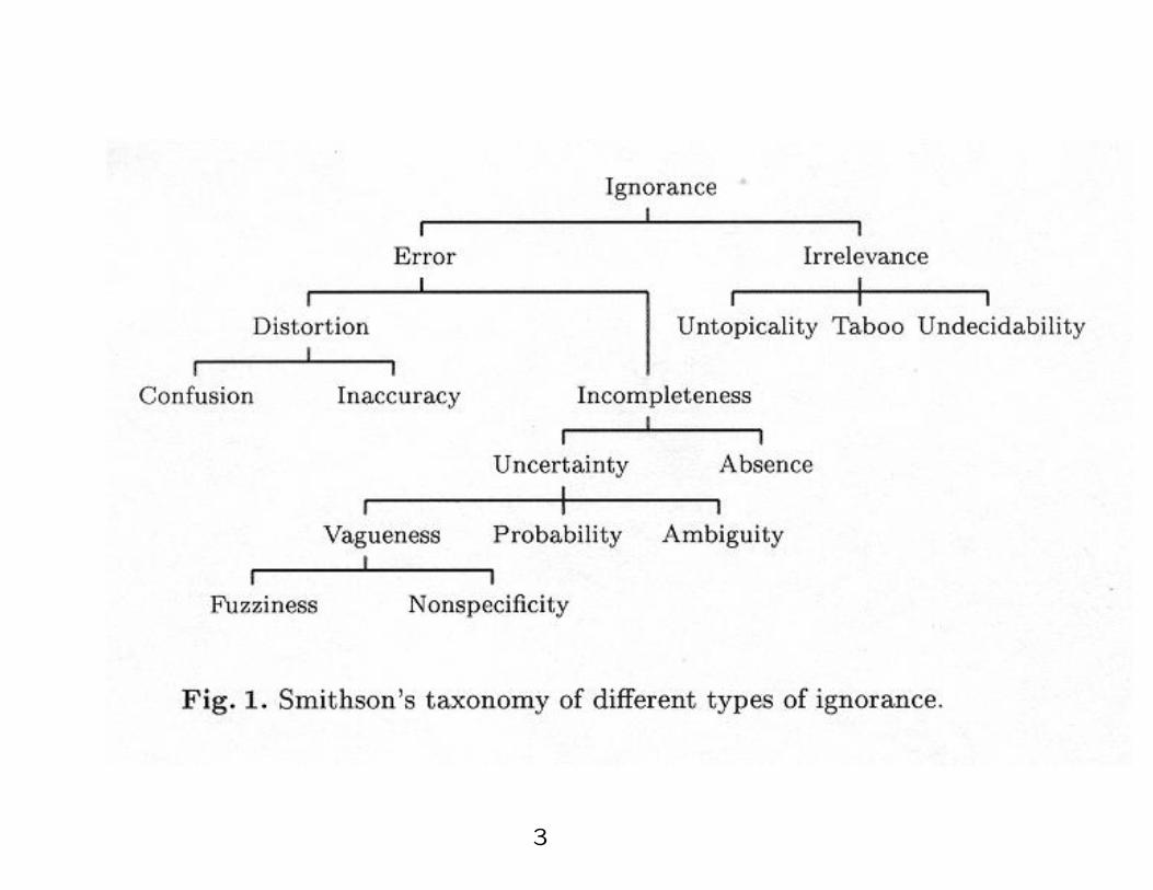
1 - Ignorance, uncertainty, distortion, inaccuracy,
vagueness, etc.
• Practical AI systems are constrained to deal with imperfect
knowledge and are thus said to reason approximately under
conditions of ingnorance
• The concept of uncertainty can be understood in the context
of ignorance.
• A taxonomy of ignorance was created by Smithson a.
aM. Smithson, Ignorance and uncertainty: Emerging Paradigms. Springer-
Verlag. New York 1989.
2
3

2 - The taxonomy are not well established
• According to Philippe Smets imprecision, inconsistency and
uncertainty are imperfect information types.
• Imprecision and inconsistency are properties related to the
content of of the statement, i.e., they are properties of the
information.
• Uncertainty is a property that results from a lack of
information about the world for deciding if the statement is
true or false, i.e., it is a property between the information and
our knowledge about the world.
4

3 - Imprecision x Uncertainty
• John has at least two children am I am sure about it. Number
of children is imprecise but certain.
• John has three children but I am not sure about it. Number of
children is precise but uncertain.
5

4 - Uncertainty x Information
According to George Klir:
• Uncertainty: result of some information deficiency
• Information: uncertainty reduction.
6
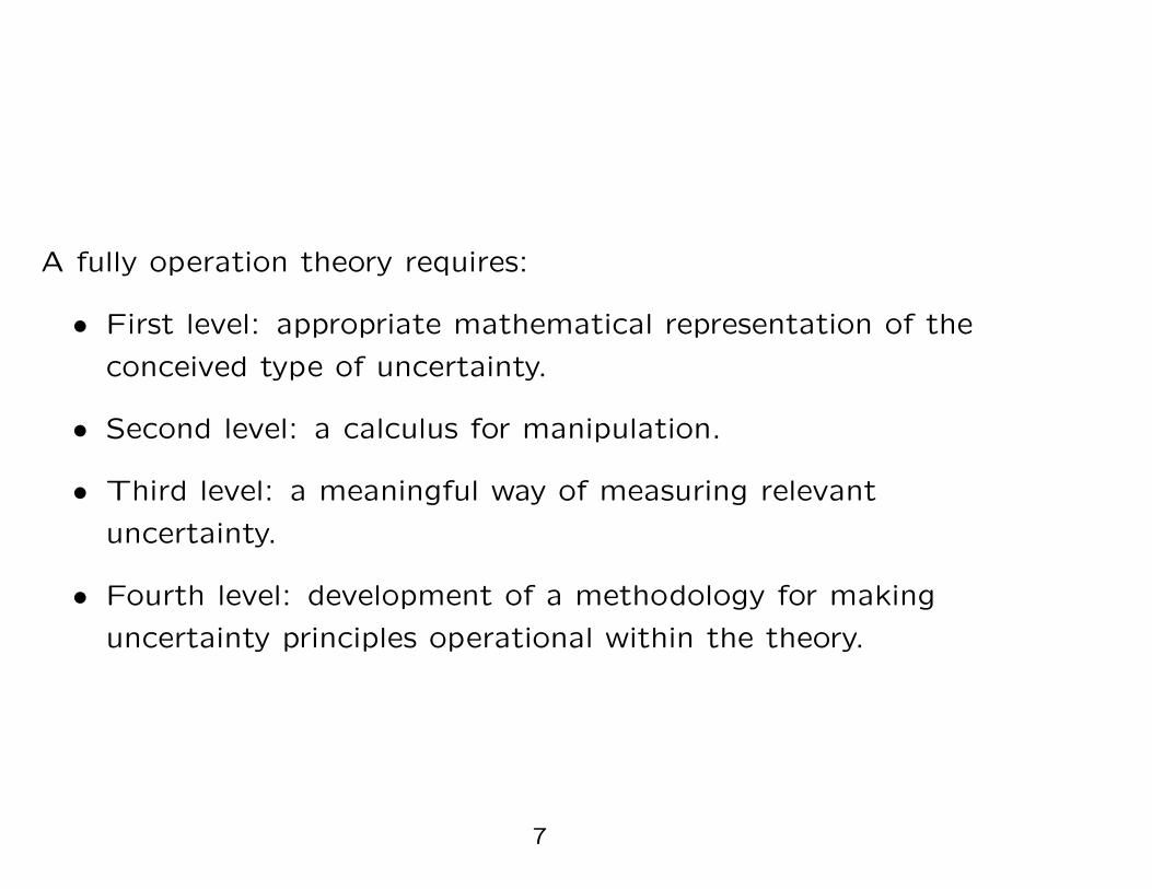
A fully operation theory requires:
• First level: appropriate mathematical representation of the
conceived type of uncertainty.
• Second level: a calculus for manipulation.
• Third level: a meaningful way of measuring relevant
uncertainty.
• Fourth level: development of a methodology for making
uncertainty principles operational within the theory.
7
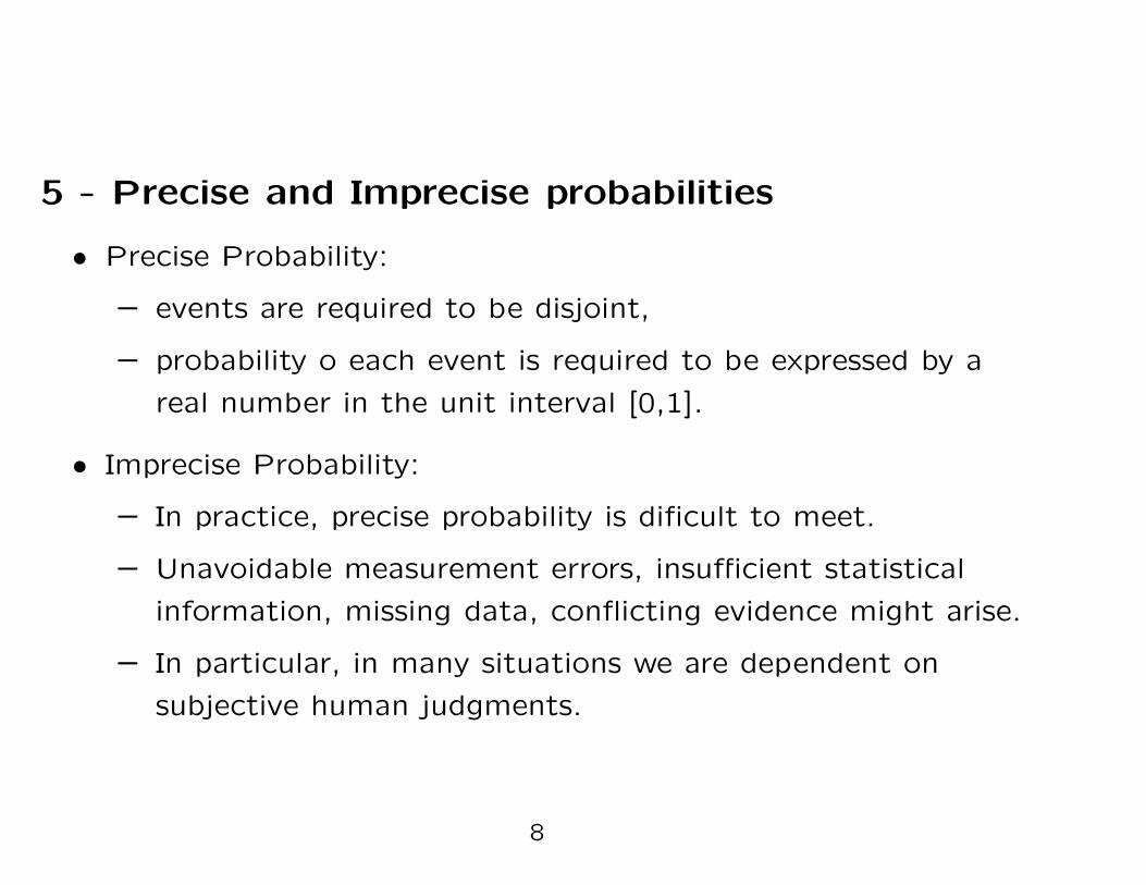
5 - Precise and Imprecise probabilities
• Precise Probability:
– events are required to be disjoint,
– probability o each event is required to be expressed by a
real number in the unit interval [0,1].
• Imprecise Probability:
– In practice, precise probability is dificult to meet.
– Unavoidable measurement errors, insufficient statistical
information, missing data, conflicting evidence might arise.
– In particular, in many situations we are dependent on
subjective human judgments.
8

6 - Imprecise probabilities: are they real ?
• The first throughout study of imprecise probability was taken
by Peter Walley a (1991).
• The main result: reasoning and decision making based on
imprecise probabilities satisfy the principle of coherence and
avoidance of sure loss, which are generally viewed as principles
of rationality.
• Hence, the requirement of precision (or equivalently, the
additivity axiom) cannot be justified as inevitable for
rationality.
aPeter Walley, Statistical reasoning with imprecise probabilities, Chapman-Hall,
1991.
9
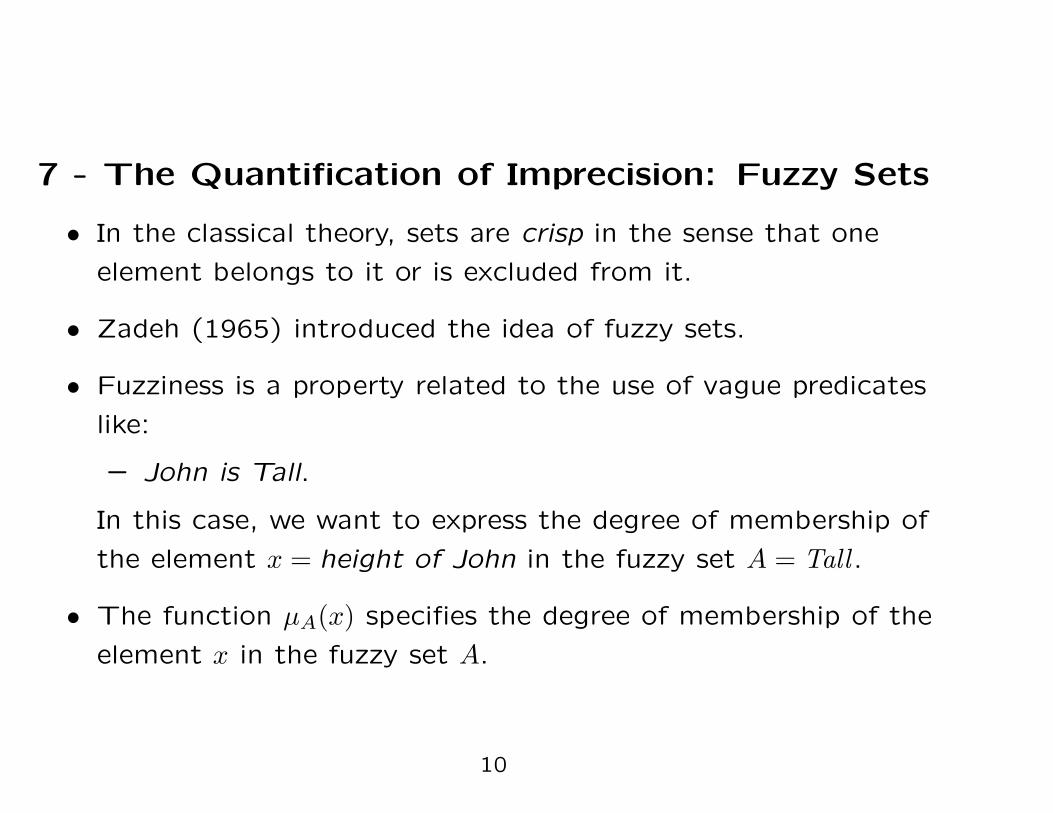
7 - The Quantification of Imprecision: Fuzzy Sets
• In the classical theory, sets are crisp in the sense that one
element belongs to it or is excluded from it.
• Zadeh (1965) introduced the idea of fuzzy sets.
• Fuzziness is a property related to the use of vague predicates
like:
– John is Tall.
In this case, we want to express the degree of membership of
the element x = height of John in the fuzzy set A = Tall.
• The function µA(x) specifies the degree of membership of the
element x in the fuzzy set A.
10
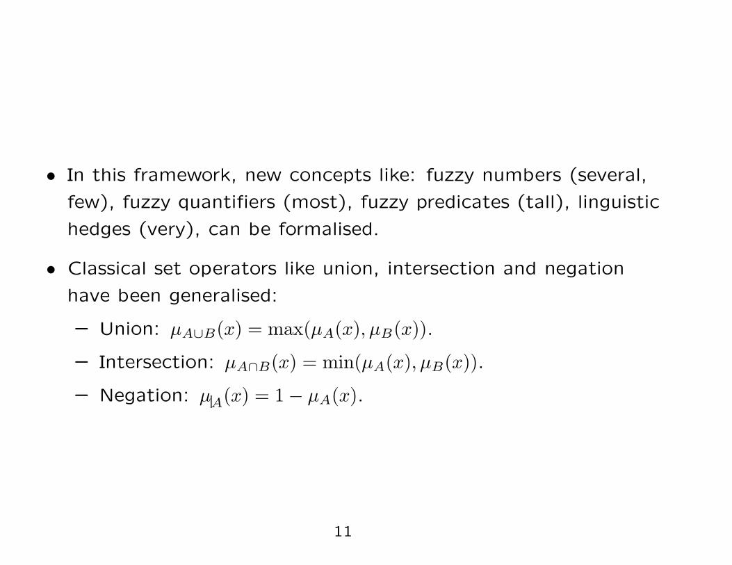
• In this framework, new concepts like: fuzzy numbers (several,
few), fuzzy quantifiers (most), fuzzy predicates (tall), linguistic
hedges (very), can be formalised.
• Classical set operators like union, intersection and negation
have been generalised:
– Union: µA∪B(x) = max(µA(x), µB(x)).
– Intersection: µA∩B(x) = min(µA(x), µB(x)).
– Negation: µA(x) = 1 − µA(x).
11

8 - The Quantification of Uncertainty: Sugeno’s
Fuzzy Measures
• Another concept developed by Sugeno (1977) received the
label fuzzy.
• Sugeno studied functions that express uncertainty with a
statement
x belongs to S,
where S is a crisp set and x is a particular arbitrary element of
the universe Ω.
• The fuzzy measure is a function
g : 2Ω → [0, 1]. (1)
Where 2Ω is the power set of crisp subsets of the universe Ω.
12
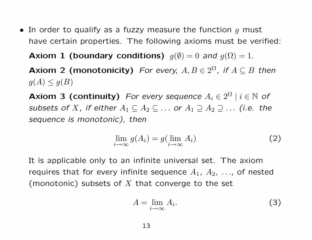
• In order to qualify as a fuzzy measure the function g must
have certain properties. The following axioms must be verified:
Axiom 1 (boundary conditions) g(∅) = 0 and g(Ω) = 1.
Axiom 2 (monotonicity) For every, A, B ∈ 2Ω, if A ⊆ B then
g(A) ≤ g(B)
Axiom 3 (continuity) For every sequence Ai ∈ 2Ω | i ∈ N of
subsets of X, if either A1 ⊆ A2 ⊆ . . . or A1 ⊇ A2 ⊇ . . . (i.e. the
sequence is monotonic), then
limi→∞
g(Ai) = g( limi→∞
Ai) (2)
It is applicable only to an infinite universal set. The axiom
requires that for every infinite sequence A1, A2, . . ., of nested
(monotonic) subsets of X that converge to the set
A = limi→∞
Ai. (3)
13

• The concept of fuzzy measure fits probability measures,
necessity measures, belief functions, etc.
• It has been called fuzzy measure but should not be confused
with fuzzy sets.
14
9 - Belief and Plausibility Measures
• The theory of Belief functions provides one way to use
mathematical probability in subjective judgement.
• It was pioneered by Dempster a (1967) and Shafer b (1976).
• It is a generalisation of the Bayesian theory of subjective
probability.
• When we use Bayesian theory to quantify judgements about a
question, we must assign probabilities to the possible answers
to that question.
• The theory of Belief is more flexible, it allows us to derive
degrees of belief for a question from probabilities for a related
question.
aA.P. Dempster, Upper and lower probabilities induced by a multivalued map-
ping, Annals of mathematical Statistics, 38, 325–339, 1967.bG. Shafer, A mathematical theory of evidence, Princeton University Press,
1976.
15
10 - Basic Probability Assignment
• Let q be a variable and Ω be the set of all possible values of q.
• The propositions can be represented as:
– The value of q is in A, where A ⊆ Ω.
• In the Dempster-Shafer theory, Ω is the frame of discernment.
• In Probability theory, it is necessary to designate the degree of
belief for each one of the elements of Ω.
• In Belief theory, the probability assignment is not made over Ω,
but on the space of all subsets of Ω, which is denoted by 2Ω.
• Let m : 2Ω → [0, 1], be a basic assignment of probability function
such that:
1. m(∅) = 0,
16

2.∑
A⊆2Ω
m(A) = 1. (4)
• m is the degree of evidence that X belongs to the set A.
• (Ω, m) is defined as the body of evidence.
• The following figure illustrates these concepts.
17

• A hydraulic analogy is used illustrate the basic probability
assignment.
• m(J, S) 6= 0 means that there is a belief that can be assigned
to J, S, but there is no further evidence for a finer
distribution.18

11 - Where is John’s wallet ?
• John has had a very hectic morning visiting three different
places; L1, L2 and L3. In the afternoon, while driving him to
the train station, he has realised that he lost his wallet, but he
is sure that he let the wallet in one of the three places where
he has been, but does not know where exactly. He has left for
his destiny but asked me to help him find his wallet.
• Knowing that the wallet is on one the three places, our frame
of discernment is Ω = L1, L2, L3.
• As John has not informed any other information, like the order
which he visited the places, we are in a complete ignorance
state.
• In this context, the basic probability assignment must be
m(L1, L2, L3) = 1 and for any other subset A ⊂ Ω we must
have m(A) = 0.
19
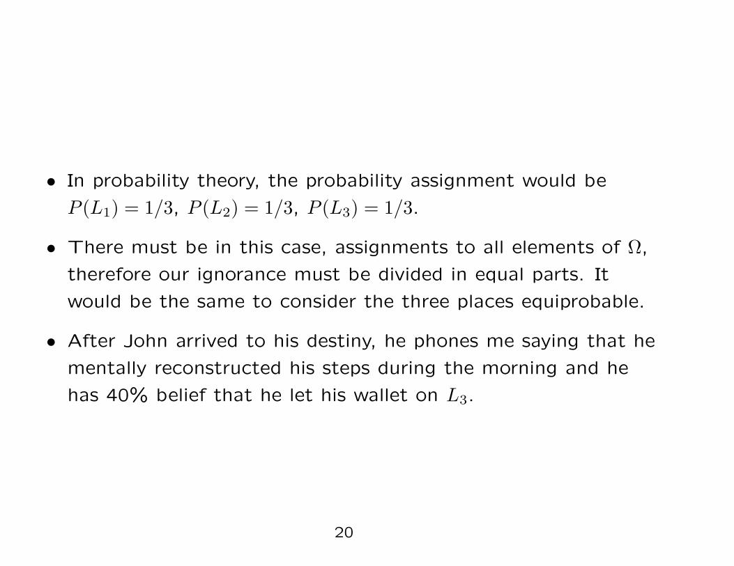
• In probability theory, the probability assignment would be
P (L1) = 1/3, P (L2) = 1/3, P (L3) = 1/3.
• There must be in this case, assignments to all elements of Ω,
therefore our ignorance must be divided in equal parts. It
would be the same to consider the three places equiprobable.
• After John arrived to his destiny, he phones me saying that he
mentally reconstructed his steps during the morning and he
has 40% belief that he let his wallet on L3.
20
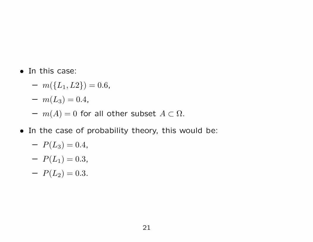
• In this case:
– m(L1, L2) = 0.6,
– m(L3) = 0.4,
– m(A) = 0 for all other subset A ⊂ Ω.
• In the case of probability theory, this would be:
– P (L3) = 0.4,
– P (L1) = 0.3,
– P (L2) = 0.3.
21

• A belief measure is a function:
Bel : 2Ω → [0, 1], (5)
which can be defined as:
Bel(A) =∑
B⊆A
m(B). (6)
• It satisfies axioms 1-3 of fuzzy measures and the following
axiom:
Bel(A1 ∪ A2 ∪ . . . ∪ An) ≥∑
i
Bel(Ai) −∑
i<j
Bel(Ai ∩ Aj)
+ . . . + (−1)n+1Bel(A1 ∩ A2 ∩ . . . ∩ An)
(7)
for every n ∈ N and every collection of subsets of X.
• m(A) gives the direct evidence support of A, Bel(A) is total
support, direct and indirect, of A.
22

• A plausibility measure is a function
Pl : 2Ω → [0, 1], (8)
which can be defined as:
Pl(A) =∑
B∩A6=∅
m(B). (9)
• It satisfies the axioms 1-3 and the following axiom:
Pl(A1 ∩ A2 ∩ . . . ∩ An) ≥∑
i
Pl(Ai) −∑
i<j
Pl(Ai ∪ Aj)
+ . . . + (−1)n+1Pl(A1 ∪ A2 ∪ . . . ∪ An)
(10)
for every n ∈ N and every collection of subsets of X.
• The plausibility measure is the sum of all basic probability
assignment of all subsets with non null intersection with A.
• Therefore, it measures the maximum belief that can be
credited to A.23

12 - Some properties
• It is easy to note that Pl(A) ≥ Bel(A).
• Similarly, Bel(¬A) indicates the total support to ¬A and Pl(¬A)
measures the plasubility of ¬A.
• As Belief and Plausibility functions are dual measures then:
– Pl(A) = 1 − Bel(¬A),
– Bel(A) = 1 − Pl(¬A).
• This can be represented by the following figure.
24

25

13 - Combining Evidences
• Evidences from two different independent sources inside the
same frame of discernment Ω can be combined
• Dempster’s Rule of Combination:
m1,2(A) =
∑
B∩C=A m1(B)m2(C)
1 − K(11)
for A 6= ∅, where
K =∑
B∩C=∅
m1(B)m2(C). (12)
• This can be illustrated by the following figure.
26

27

14 - Who murdered Karen ?
• Four persons are locked in a room: Bob, Jim, Sally and Karen.
Suddenly, there is a electricity shortage supply and the room
become dark. When the electricity supply is normalised Bob,
Jim and Sally realises that Karen is dead. A police inspector
arrives and concludes that Karen was murdered, and the
murder is one of the three persons.
• After detailed investigation and based on evidences found in
the room, the inspector produces a basic probability
assignment which reflects his beliefs and doubts.
28
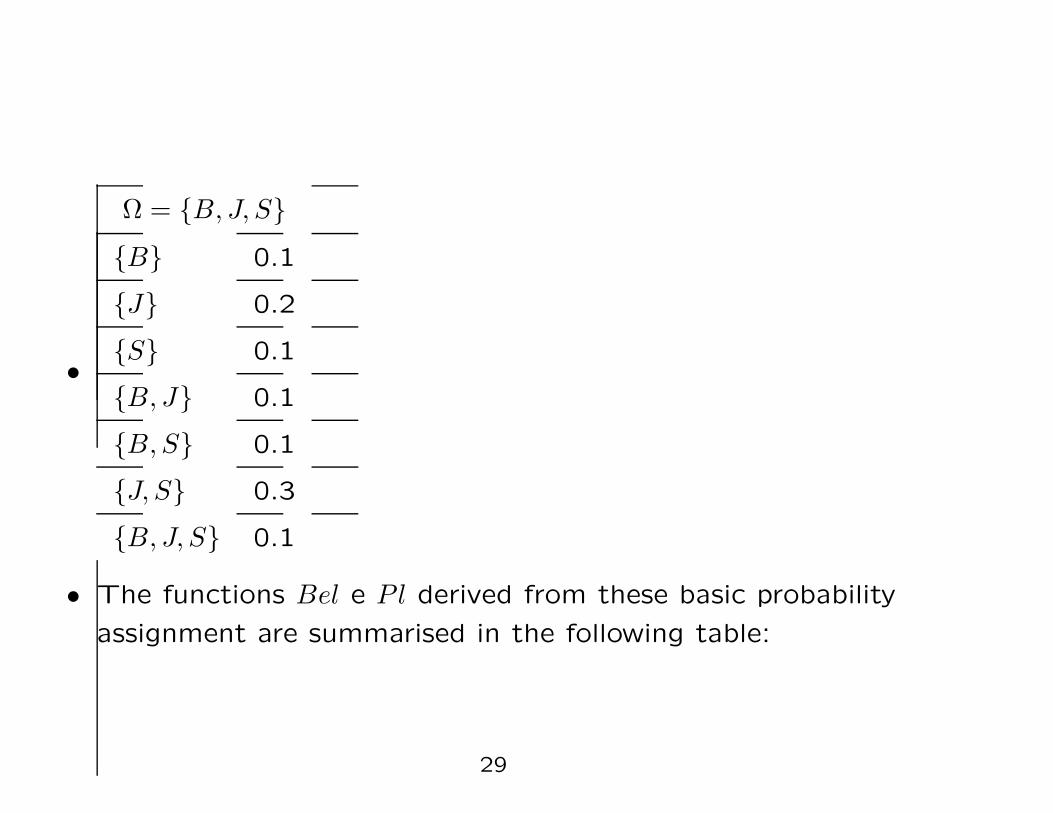
•
Ω = B, J, S
B 0.1
J 0.2
S 0.1
B, J 0.1
B, S 0.1
J, S 0.3
B, J, S 0.1
• The functions Bel e Pl derived from these basic probability
assignment are summarised in the following table:
29

m1 Bel1 Pl1
B 0.1 0.1 0.4
J 0.2 0.2 0.7
S 0.1 0.1 0.6
B, J 0.1 0.4 0.9
B, S 0.1 0.3 0.8
J, S 0.3 0.6 0.9
B, J, S 0.1 1.0 1.0
• It is easy to verify that Jim is the main suspect, but the
hypothesis of Sally being the murderer is very plausible
Pl(S) = 0.6.
• Later, based on further evidence, information about the dead
and her personal relationships with the suspects, the inspector
builds up another basic probability assignment m2.
30

•
m1 : 2Ω → [0, 1]
Ω = B, J, S
B 0.1
J 0.2
S 0.1
B, J 0.1
B, S 0.1
J, S 0.3
B, J, S 0.1
m2 : 2Ω → [0, 1]
Ω = B, J, S
B 0.2
J 0.1
S 0.05
B, J 0.05
B, S 0.3
J, S 0.1
B, J, S 0.2
• Now, using the Dempster’s rule the beliefs of both evidences
can be combined in a new basic probability assignment m12.
• The
following figure illustrates the combination of the two evidences.
31

32

• The results for m12, Bel12, Pl12 are summarised in the following
table.
m12 Bel12 Pl12
B 0.225 0.225 0.4
J 0.219 0.219 0.485
S 0.25 0.25 0.451
B, J 0.04 0.515 0.781
B, S 0.105 0.549 0.751
J, S 0.131 0.6 0.775
B, J, S 0.03 1.0 1.0
33

15 - The Classical Probability Measure
• When the axiom for belief measures is replaced with a stronger
axiom:
Bel(A ∪ B) = Bel(A) + Bel(B), (13)
whenever A ∩ B = ∅ we obtain a special type of belief measures
the classical probability measures.
34
16 - There are many possible interpretations for
probabilities
• The classical theory: as defended by Laplace, assumes the
existence of a fundamental set of equipossible events.
• The relative frequency theory: in this case, probability is
essentially the convergence limit of relative frequencies under
repeated independent trials.
• The subjective (or Bayesian) probability: in this case the
probability measure quantifies the credibility that an event will
occur. It is a subjective, personal measure.
35

17 - The Kolmogorov’s axioms
Definition 1 Let Ω be a set of mutually exclusive events.
Definition 2 let F be a set of subsets of Ω such that:
1. Ω ∈ F ,
2. E1,E2 ∈ F ⇒ E1 ∪ E2 ∈ F ,
3. E ∈ F ⇒ ¬E ∈ F .
then F is defined by event algebra related Ω.
36

Definition 3 Let Ω, F and a function P which associates a real
number to each E ∈ F If P satisfies the following axioms:
1. P (E) ≥ 0 ∀E ∈ F ,
2. P (Ω) = 1,
3. If E1 e E2 are two subsets with E1 ∩ E2 = ∅ then
P (E1 ∪ E2) = P (E1) + P (E2). The triple (Ω, F, P ) are defined as
probability space, and P is the probability measure of F .
37

18 - Some consequences
• According to the third axiom, the probability associated to any
set of events its the sum of probabilities of its disjoint
components.
• Any event event A can be written as (A ∪ B) ∪ (A ∩ ¬B)),
therefore we have:
P (A) = P (A ∪ B) + P (A ∩ ¬B) (14)
.
• This can be extended to n mutually exclusive events
B1, B2, . . . , Bn,
P (A) =n
∑
i=1
P (A ∪ Bi). (15)
• A direct consequence of this argument is:
P (A) + P (¬A) = 1. (16)
38
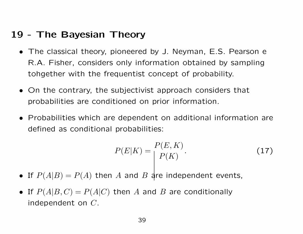
19 - The Bayesian Theory
• The classical theory, pioneered by J. Neyman, E.S. Pearson e
R.A. Fisher, considers only information obtained by sampling
tohgether with the frequentist concept of probability.
• On the contrary, the subjectivist approach considers that
probabilities are conditioned on prior information.
• Probabilities which are dependent on additional information are
defined as conditional probabilities:
P (E|K) =P (E, K)
P (K). (17)
• If P (A|B) = P (A) then A and B are independent events,
• If P (A|B, C) = P (A|C) then A and B are conditionally
independent on C.
39
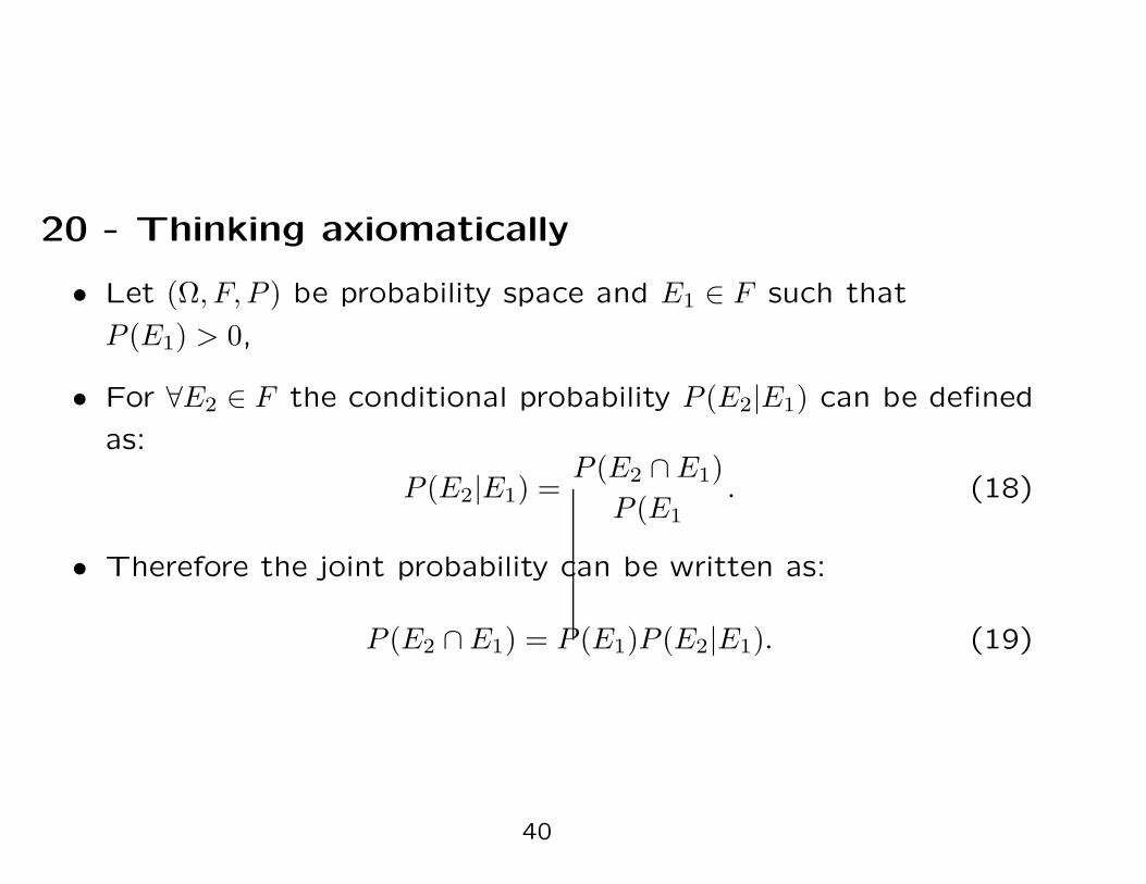
20 - Thinking axiomatically
• Let (Ω, F, P ) be probability space and E1 ∈ F such that
P (E1) > 0,
• For ∀E2 ∈ F the conditional probability P (E2|E1) can be defined
as:
P (E2|E1) =P (E2 ∩ E1)
P (E1
. (18)
• Therefore the joint probability can be written as:
P (E2 ∩ E1) = P (E1)P (E2|E1). (19)
40

• The probability of an event A can be calculated conditioned on
a mutually exclusive set of events B1, B2, . . . , Bn:
P (A) =n
∑
i=1
P (A|Bi)P (Bi). (20)
• It is possible to write the a posteriori probability as:
P (E2|E1) =P (E1|E2)P (E2)
P (E1). (21)
41

21 - Understanding the Bayesian concept in
probabilistic diagrams
• Starting from:
– P (H) = h, P (¬H) = 1 − h,
– P (E|H) = e1/h, P (E|¬H) = e2/(1 − h).
• What does it mean the shadowed area in the figure ?
42
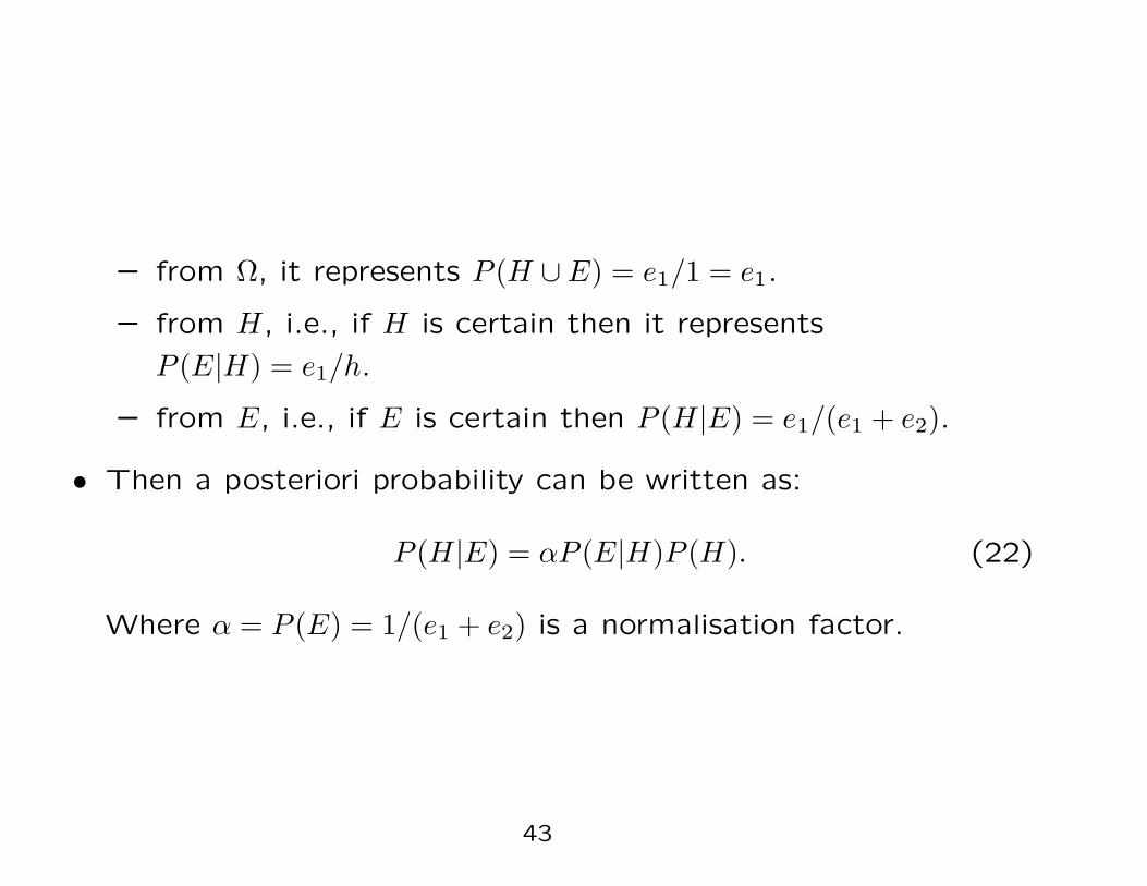
– from Ω, it represents P (H ∪ E) = e1/1 = e1.
– from H, i.e., if H is certain then it represents
P (E|H) = e1/h.
– from E, i.e., if E is certain then P (H|E) = e1/(e1 + e2).
• Then a posteriori probability can be written as:
P (H|E) = αP (E|H)P (H). (22)
Where α = P (E) = 1/(e1 + e2) is a normalisation factor.
43

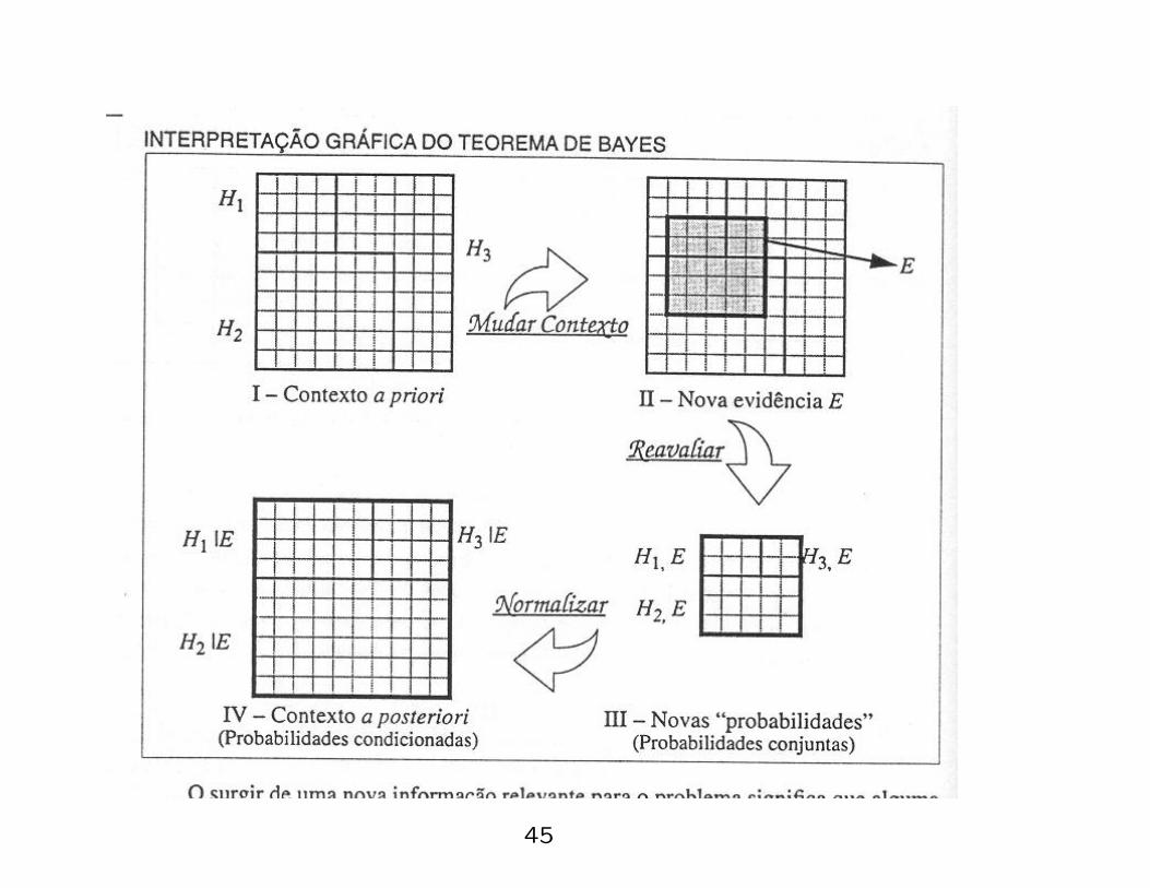
22 - The Bayes theorem
• Given the probabilistic space (Ω, F, P ) and a set F of mutually
exclusive events H1, H2, . . . , Hn with non null probabilities,
then:
P (Hj |E) =P (E|Hj)P (Hj)
∑ni=1
P (E|Hi)P (Hi)(23)
• This can be summarised in the following figure:
44
45

23 - Bayesian networks
• A Bayesian network is a graphical representation of a
probability distribution.
• Each Bayesian network is comprised of two distinct parts:
1. A directed acyclic graph,
2. a set of probability tables.
• Edges represent direct causal influences between variables, i.e.,
conditional independence.
• it is a parsimonious representation.
• It is possible to infer things like: given that D is true What
state is the most probable state for B or C ?
• This is illustrated in the following example:
46

47

48
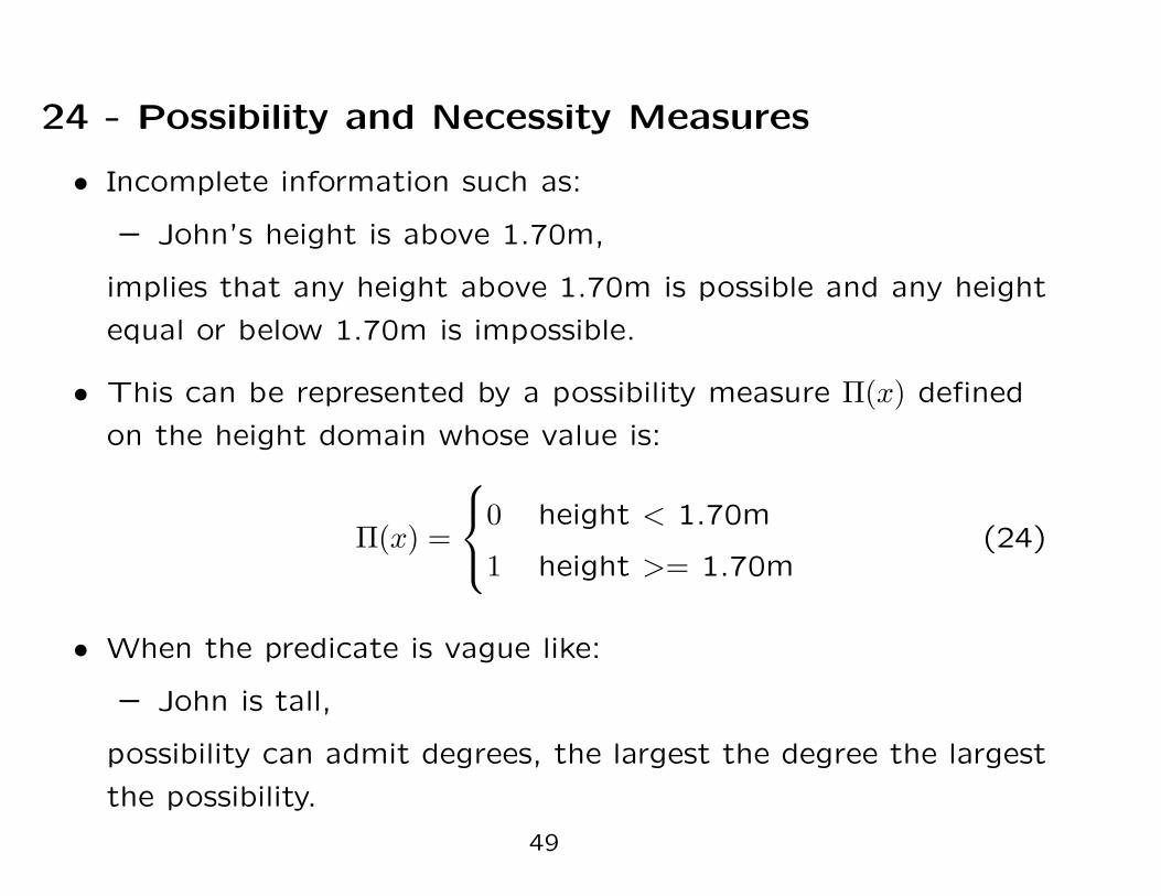
24 - Possibility and Necessity Measures
• Incomplete information such as:
– John’s height is above 1.70m,
implies that any height above 1.70m is possible and any height
equal or below 1.70m is impossible.
• This can be represented by a possibility measure Π(x) defined
on the height domain whose value is:
Π(x) =
0 height < 1.70m
1 height >= 1.70m(24)
• When the predicate is vague like:
– John is tall,
possibility can admit degrees, the largest the degree the largest
the possibility.
49

• Possibility is usually associated with fuzziness, however,
non-fuzzy (crisp) events can admit different degrees of
possibility. Suppose that there is a box where you try to
squeeze soft balls. You can say:
– It is possible to put 20 balls in it, impossible to put 30 balls in
it, quite possible to put 24 balls, but not so possible to put 26
balls, . . .
These degrees of possibility are degrees of realizability and
totally unrelated to any underlying random process.
50

A salesman could also forecast about next year sales. He could
say:
– It is possible to sell about 50K, impossible to sell more than
100K, quite possible to sell 70K, hardly possible to sell more
than 90K, . . .
This might express the possible values of sales based on the
sale capacity. On the contrary, he could express what he will
actually sell next year, but this concerns another problem for
which the theories of probability and belief functions are more
adequate.
51

25 - Possibility and Necessity Measures: the
definition
• Let Π and N denote a possibility and a necessity measure on
2Ω, respectively. Then,
Π(A ∪ B) = max[Π(A), Π(B)] (25)
and
N(A ∩ B) = min[N(A), N(B)] (26)
for all A, B ∈ 2Ω.
• The necessity and possibility measures are dual measures.
• Let E ⊆ X a certain event, then we can define:
ΠE(A) =
1 A ∩ E 6= ∅
0 A ∪ E = ∅(27)
ΠE(A) = 1 means that A is a possible event.
52

• If A and ¬A are two complementary events then,
max(Π(A), Π(¬A)) = 1. (28)
If two events are complementary at least one of them is
possible.
• Let E ⊆ X a certain event, then we can define:
NE(A) =
1 A ⊆ E
0 A ⊃ E(29)
NE(A) = 1 means that A is a certain event, i.e., necessarily
true.
• They are related to each other by the equation
N(A) = 1 − Π(¬A), (30)
for all A ∈ 2Ω.
53

• Π(A) is the degree of possibility that A is true.
• The necessity of a proposition is the negation of the possibility
of its negation.
• An event is necessary when the occurrence of its negation is
impossible.
• An equivalent argument could be:
min(N(A), N(¬A)) = 0. (31)
Which means that an event and its negation cannot be
necessary simultaneously.
• Using intuition an event must be possible before being
necessary, threfore:
Π(A) ≥ N(A) (32)
• It is easy to note that:
1. N(A) > 0 → Π(A) = 1
54
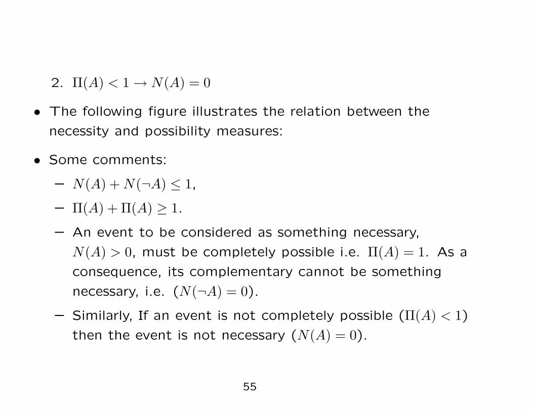
2. Π(A) < 1 → N(A) = 0
• The following figure illustrates the relation between the
necessity and possibility measures:
• Some comments:
– N(A) + N(¬A) ≤ 1,
– Π(A) + Π(A) ≥ 1.
– An event to be considered as something necessary,
N(A) > 0, must be completely possible i.e. Π(A) = 1. As a
consequence, its complementary cannot be something
necessary, i.e. (N(¬A) = 0).
– Similarly, If an event is not completely possible (Π(A) < 1)
then the event is not necessary (N(A) = 0).
55

56
• Every possibility measure Π on P(X) can be uniquely
determined by a possibilistic distribution function:
π : X → [0, 1] (33)
via the formula:
Π(A) = maxx∈A
π(x). (34)
57

26 - Possibility x Probability
• Consider the following statement:
– Hans ate X eggs for breakfast, with X ∈ 1, . . . , 8
• We can associate both a possibility distribution (based on our
view o ease which Hans can eat eggs) and a probability
distribution (based on our observations of Hans at breakfast).
• We could have:
u 1 2 3 4 5 6 7 8
ΠX(u) 1 1 1 1 0.8 0.6 04 0.2
PrX(u) 0.1 0.8 0.1 0 0 0 0 0
• So, while is perfectly possible that Hans can eat three eggs for
breakfast, he is unlikely to do so.
58

• There is a heuristic connection between possibility and
probability, since if something is impossible it is likely to be
improbable.
• A high degree of possibility does not imply a high degree of
probability, nor a low degree of probability reflect a low degree
of possibility.
59
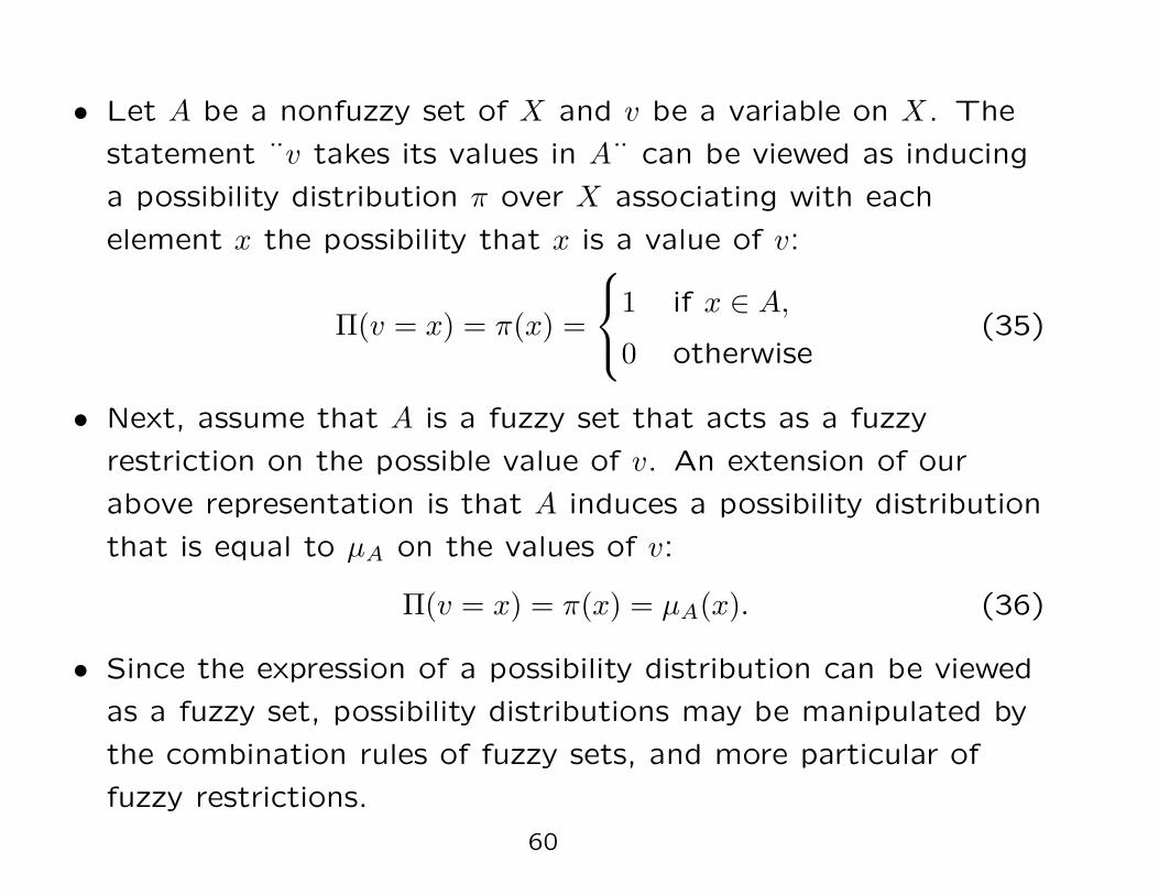
• Let A be a nonfuzzy set of X and v be a variable on X. The
statement ¨v takes its values in A¨ can be viewed as inducing
a possibility distribution π over X associating with each
element x the possibility that x is a value of v:
Π(v = x) = π(x) =
1 if x ∈ A,
0 otherwise(35)
• Next, assume that A is a fuzzy set that acts as a fuzzy
restriction on the possible value of v. An extension of our
above representation is that A induces a possibility distribution
that is equal to µA on the values of v:
Π(v = x) = π(x) = µA(x). (36)
• Since the expression of a possibility distribution can be viewed
as a fuzzy set, possibility distributions may be manipulated by
the combination rules of fuzzy sets, and more particular of
fuzzy restrictions.
60
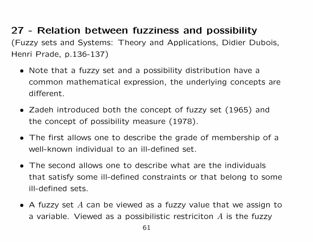
27 - Relation between fuzziness and possibility
(Fuzzy sets and Systems: Theory and Applications, Didier Dubois,
Henri Prade, p.136-137)
• Note that a fuzzy set and a possibility distribution have a
common mathematical expression, the underlying concepts are
different.
• Zadeh introduced both the concept of fuzzy set (1965) and
the concept of possibility measure (1978).
• The first allows one to describe the grade of membership of a
well-known individual to an ill-defined set.
• The second allows one to describe what are the individuals
that satisfy some ill-defined constraints or that belong to some
ill-defined sets.
• A fuzzy set A can be viewed as a fuzzy value that we assign to
a variable. Viewed as a possibilistic restriciton A is the fuzzy
61

set of nonfuzzy values that can be possibly assigned to v.
• For instance, µTall (x) quantifies the membership of a person
with height h to the set of Tall men and πTall(h) quantifies the
possibility that the height of a person is h given the person
belongs to the set of Tall men.
62

• Zadeh’s possibilistic principle postulates the following equality:
πTall (h) = µTall (h), ∀h ∈ H, (37)
where H is the set of height.
• The writing is often confusing and would have been better
written as:
π(h|Tall) = µ(Tall |h), ∀h ∈ H, (38)
or still better: If µ(Tall |h) = x then π(h|Tall) = x
• The difference is analogous to the difference between a
probability distribution p(x|θ) (the probability of the observation
x given the hypothesis θ) and a likelihood function l(θ|x (the
likelihood of the hypothesis θ given the observation x).
63

28 - The following figure illustrates the states of
knowledge and uncertainty of typical propositions
64
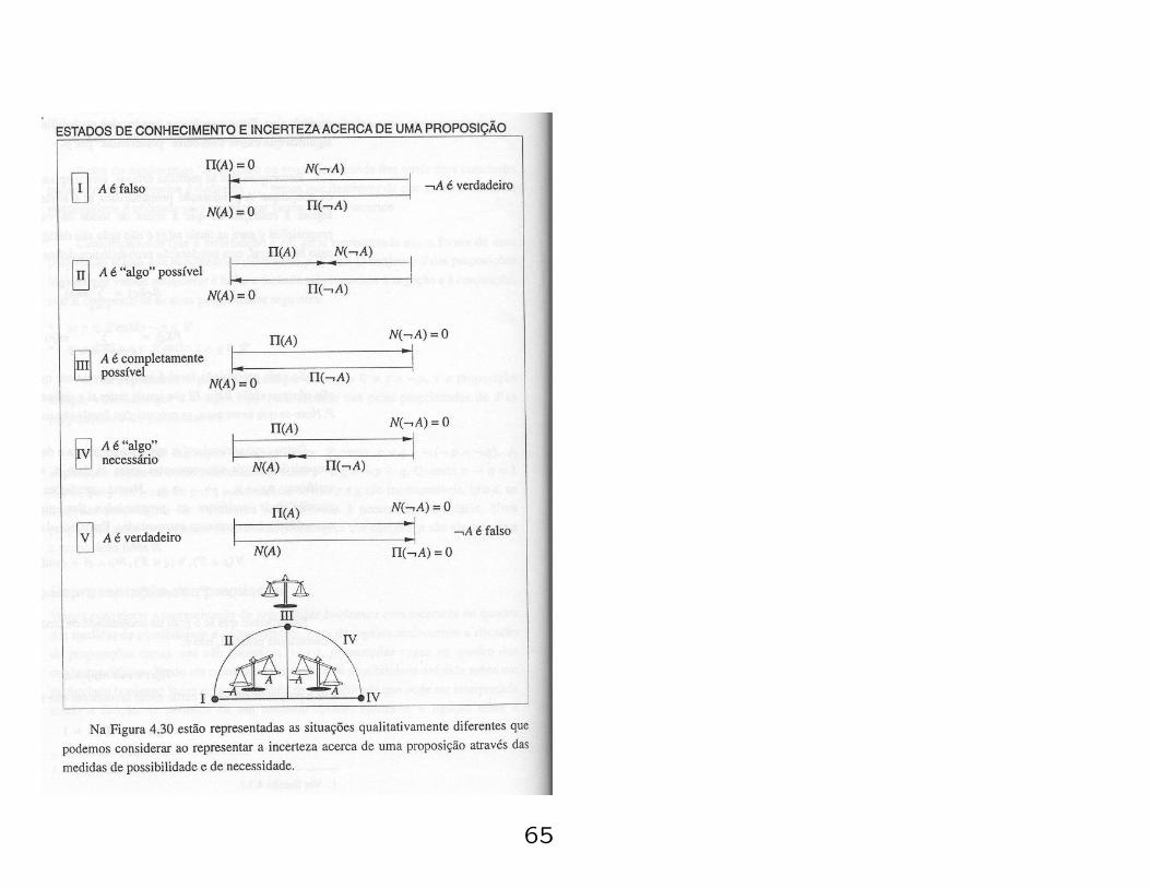
65