lable at ScienceDirect

Renewable Energy 68 (2014) 570e580

Contents lists avai

Renewable Energy

journal homepage: www.elsevier .com/locate/renene

Uncertainty analysis of wave energy farms financial indicators

R. Guanche*, A.D. de Andrés, P.D. Simal, C. Vidal, I.J. LosadaInstituto de Hidráulica Ambiental e IH Cantabria, Universidad de Cantabria, C/Isabel Torres 15, Parque Científico y Tecnológico de Cantabria,39011 Santander, Spain

a r t i c l e i n f o

Article history:Received 29 July 2013Accepted 25 February 2014Available online

Keywords:Wave interactionWave energy converterInternal rate of returnNet present valueUncertainty

* Corresponding author. Tel.: þ34 942 201 616; faxE-mail addresses: rguanche@gmail.com, guancher

http://dx.doi.org/10.1016/j.renene.2014.02.0460960-1481/� 2014 Elsevier Ltd. All rights reserved.

a b s t r a c t

In this work, an analysis of the uncertainty that influences wave energy farm financial returns is carriedout. Firstly, a methodology to analyze the financial uncertainty through cash flow analysis is developed. Areconstruction of a set of power production life-cycles is made based on the methodology proposed inRef. [1] using a selection and an interpolation technique. This set of lifecycles allowed to obtain thestatistical distributions of the main financial indicators (IRR, NPV and PBP). The high variability of theseparameters is explained by the climate variability. Therefore, for the economic study of a wave energyproject the influence of the climate conditions is demonstrated and for this purpose a long climate dataseries is needed. Finally, a second uncertainty source related with the political and legislation environ-ment is studied, focusing on the effect of feed in tariff. This sensitivity analysis of the feed in tariffs ismade based on cash-flow algorithm. Current feed in tariffs seemed insufficient in order to get profitablewave energy projects and also an increase in feed in tariff resulted in an increase of variability of financialindicators. Therefore an increase in feed in tariff is not recommended for early stage technologies. Finally,learning curve was also included in this investigation and it appeared as a key parameter in order to getcost effective financial returns.

� 2014 Elsevier Ltd. All rights reserved.

1. Introduction

Nowadays wave energy is still in the prototype testing stage.However, the ocean wave energy sector has significant potential tocontribute substantially to the global electricity generation if suf-ficient investment is provided (see Ref. [2]). Furthermore, waveenergy represents a good alternative as a renewable source due tothe low environmental impacts (see Ref. [3]) and the extensive sitesavailable for the placement of wave farms. Current wave energytargets for 2020 are quite ambitious (e.g. 1000 MW for 2020 in theUK or 500 MW for Ireland) making economic assessment of waveenergy farms a key issue in the search of financial resources (seeRef. [4]).

A methodology for economic analysis of wave energy projects istherefore required and it is an essential tool for assessing the po-tential profitability of wave energy projects from the perspective ofdevelopers, local administration and investors. Beside costs, de-velopers, investors and public administration’s major concern is theassessment of project uncertainties. According to Ref. [5] there are

: þ34 942 266 361.@unican.es (R. Guanche).

three major sources of uncertainty that can affect the profitabilityof an investment projects.

The first one is related to the high internal variability of the data:met-ocean historical records show a highly variable behavior (seeRef. [6]) which origins uncertainty about how seasonal, interannualand long termvariability of wave energy fluxmay affect productionover the farm’s expected life.

The second source of uncertainty has to do with the fact thatmost technologies have rarely been tested under real conditions;consequently only simulations of future response and efficiency arepossible. Future estimates should consider the reduction in un-certainties thanks to the experience acquired through the learningprocesses associated with the deployment of WECs.

The last source of uncertainty considered is linked to socioeco-nomic issues including, among others: institutional support,availability of subsidies for emerging green technologies, futuresocial acceptance or commercial conditions under which energywill be supplied to users. Therefore, a study of the uncertaintiesthat affect wave energy development is required in order to provideinvestors a guide to the potential risks assumed on wave energydevelopment.

Several authors have carried out studies regarding the economicperformance of wave energy projects ([4,7,8]), almost all of them

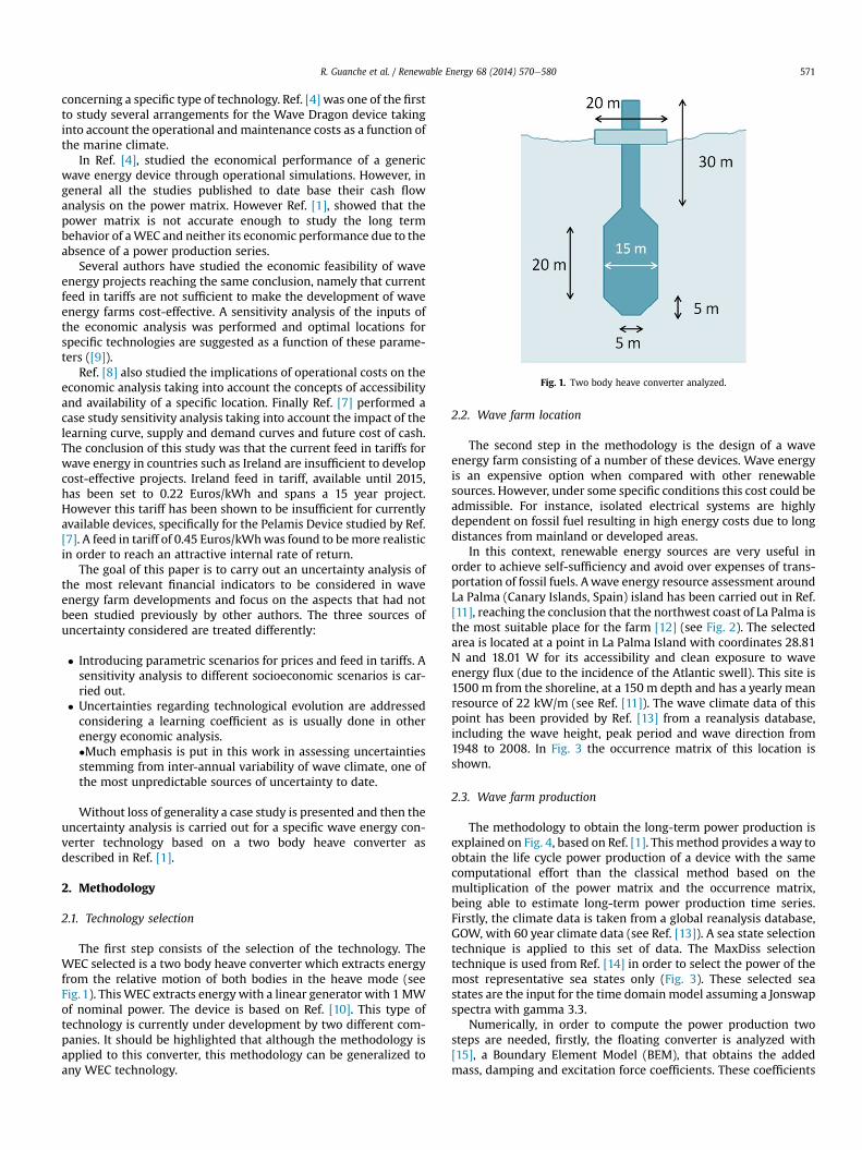
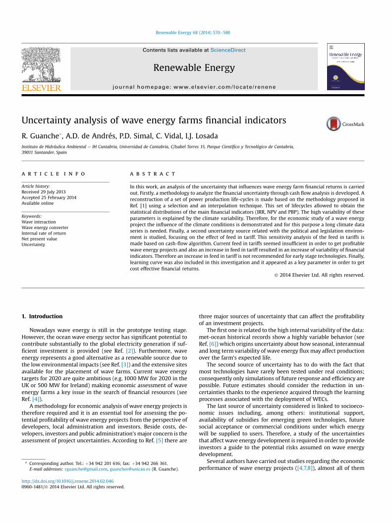
Fig. 1. Two body heave converter analyzed.

R. Guanche et al. / Renewable Energy 68 (2014) 570e580 571

concerning a specific type of technology. Ref. [4] was one of the firstto study several arrangements for the Wave Dragon device takinginto account the operational andmaintenance costs as a function ofthe marine climate.

In Ref. [4], studied the economical performance of a genericwave energy device through operational simulations. However, ingeneral all the studies published to date base their cash flowanalysis on the power matrix. However Ref. [1], showed that thepower matrix is not accurate enough to study the long termbehavior of aWEC and neither its economic performance due to theabsence of a power production series.

Several authors have studied the economic feasibility of waveenergy projects reaching the same conclusion, namely that currentfeed in tariffs are not sufficient to make the development of waveenergy farms cost-effective. A sensitivity analysis of the inputs ofthe economic analysis was performed and optimal locations forspecific technologies are suggested as a function of these parame-ters ([9]).

Ref. [8] also studied the implications of operational costs on theeconomic analysis taking into account the concepts of accessibilityand availability of a specific location. Finally Ref. [7] performed acase study sensitivity analysis taking into account the impact of thelearning curve, supply and demand curves and future cost of cash.The conclusion of this study was that the current feed in tariffs forwave energy in countries such as Ireland are insufficient to developcost-effective projects. Ireland feed in tariff, available until 2015,has been set to 0.22 Euros/kWh and spans a 15 year project.However this tariff has been shown to be insufficient for currentlyavailable devices, specifically for the Pelamis Device studied by Ref.[7]. A feed in tariff of 0.45 Euros/kWhwas found to bemore realisticin order to reach an attractive internal rate of return.

The goal of this paper is to carry out an uncertainty analysis ofthe most relevant financial indicators to be considered in waveenergy farm developments and focus on the aspects that had notbeen studied previously by other authors. The three sources ofuncertainty considered are treated differently:

� Introducing parametric scenarios for prices and feed in tariffs. Asensitivity analysis to different socioeconomic scenarios is car-ried out.

� Uncertainties regarding technological evolution are addressedconsidering a learning coefficient as is usually done in otherenergy economic analysis.�Much emphasis is put in this work in assessing uncertaintiesstemming from inter-annual variability of wave climate, one ofthe most unpredictable sources of uncertainty to date.

Without loss of generality a case study is presented and then theuncertainty analysis is carried out for a specific wave energy con-verter technology based on a two body heave converter asdescribed in Ref. [1].

2. Methodology

2.1. Technology selection

The first step consists of the selection of the technology. TheWEC selected is a two body heave converter which extracts energyfrom the relative motion of both bodies in the heave mode (seeFig. 1). ThisWEC extracts energy with a linear generator with 1MWof nominal power. The device is based on Ref. [10]. This type oftechnology is currently under development by two different com-panies. It should be highlighted that although the methodology isapplied to this converter, this methodology can be generalized toany WEC technology.

2.2. Wave farm location

The second step in the methodology is the design of a waveenergy farm consisting of a number of these devices. Wave energyis an expensive option when compared with other renewablesources. However, under some specific conditions this cost could beadmissible. For instance, isolated electrical systems are highlydependent on fossil fuel resulting in high energy costs due to longdistances from mainland or developed areas.

In this context, renewable energy sources are very useful inorder to achieve self-sufficiency and avoid over expenses of trans-portation of fossil fuels. Awave energy resource assessment aroundLa Palma (Canary Islands, Spain) island has been carried out in Ref.[11], reaching the conclusion that the northwest coast of La Palma isthe most suitable place for the farm [12] (see Fig. 2). The selectedarea is located at a point in La Palma Island with coordinates 28.81N and 18.01 W for its accessibility and clean exposure to waveenergy flux (due to the incidence of the Atlantic swell). This site is1500 m from the shoreline, at a 150 m depth and has a yearly meanresource of 22 kW/m (see Ref. [11]). The wave climate data of thispoint has been provided by Ref. [13] from a reanalysis database,including the wave height, peak period and wave direction from1948 to 2008. In Fig. 3 the occurrence matrix of this location isshown.

2.3. Wave farm production

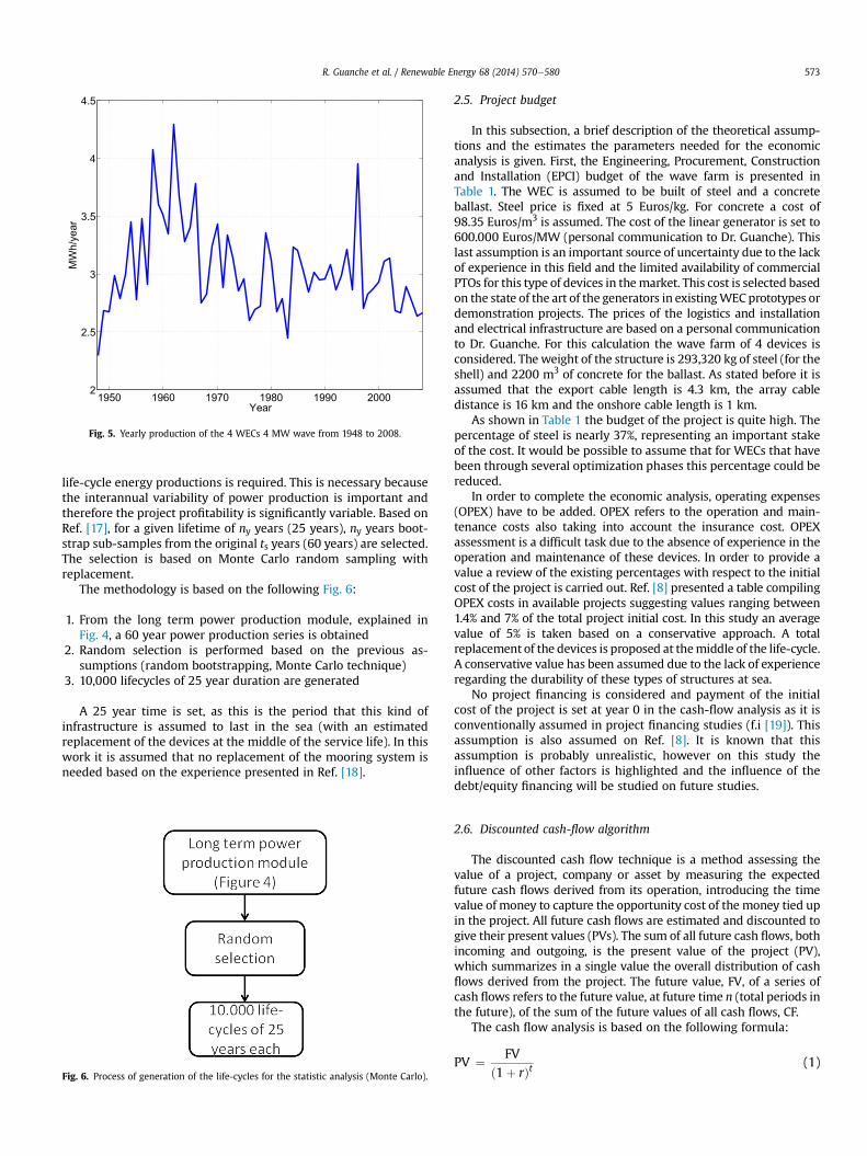
The methodology to obtain the long-term power production isexplained on Fig. 4, based on Ref. [1]. This method provides away toobtain the life cycle power production of a device with the samecomputational effort than the classical method based on themultiplication of the power matrix and the occurrence matrix,being able to estimate long-term power production time series.Firstly, the climate data is taken from a global reanalysis database,GOW, with 60 year climate data (see Ref. [13]). A sea state selectiontechnique is applied to this set of data. The MaxDiss selectiontechnique is used from Ref. [14] in order to select the power of themost representative sea states only (Fig. 3). These selected seastates are the input for the time domain model assuming a Jonswapspectra with gamma 3.3.

Numerically, in order to compute the power production twosteps are needed, firstly, the floating converter is analyzed with[15], a Boundary Element Model (BEM), that obtains the addedmass, damping and excitation force coefficients. These coefficients

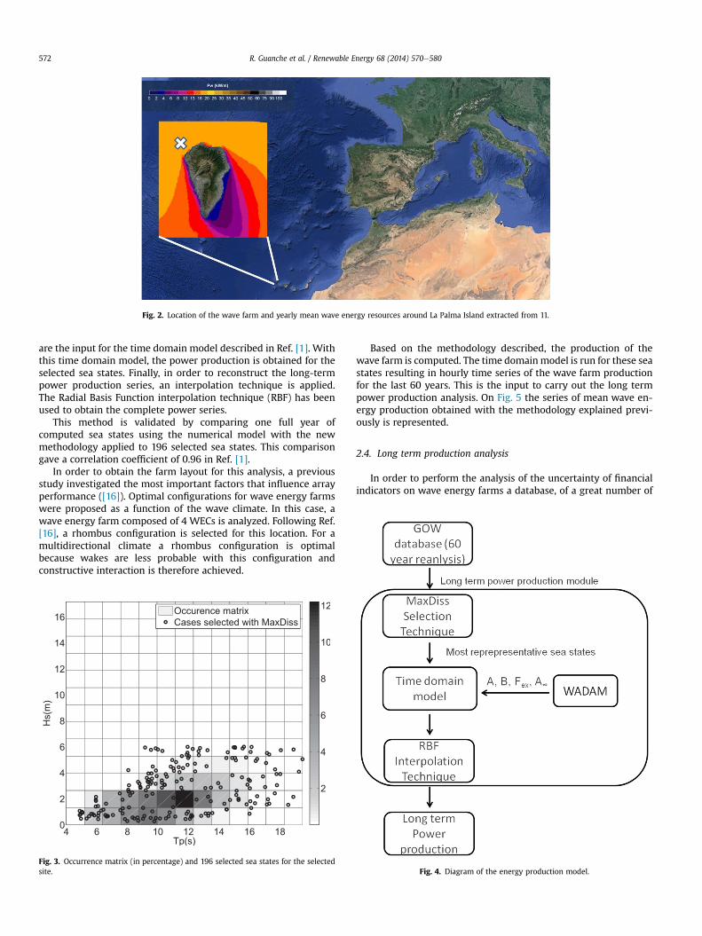
Fig. 2. Location of the wave farm and yearly mean wave energy resources around La Palma Island extracted from 11.

R. Guanche et al. / Renewable Energy 68 (2014) 570e580572

are the input for the time domain model described in Ref. [1]. Withthis time domain model, the power production is obtained for theselected sea states. Finally, in order to reconstruct the long-termpower production series, an interpolation technique is applied.The Radial Basis Function interpolation technique (RBF) has beenused to obtain the complete power series.

This method is validated by comparing one full year ofcomputed sea states using the numerical model with the newmethodology applied to 196 selected sea states. This comparisongave a correlation coefficient of 0.96 in Ref. [1].

In order to obtain the farm layout for this analysis, a previousstudy investigated the most important factors that influence arrayperformance ([16]). Optimal configurations for wave energy farmswere proposed as a function of the wave climate. In this case, awave energy farm composed of 4 WECs is analyzed. Following Ref.[16], a rhombus configuration is selected for this location. For amultidirectional climate a rhombus configuration is optimalbecause wakes are less probable with this configuration andconstructive interaction is therefore achieved.

Fig. 3. Occurrence matrix (in percentage) and 196 selected sea states for the selectedsite.

Based on the methodology described, the production of thewave farm is computed. The time domainmodel is run for these seastates resulting in hourly time series of the wave farm productionfor the last 60 years. This is the input to carry out the long termpower production analysis. On Fig. 5 the series of mean wave en-ergy production obtained with the methodology explained previ-ously is represented.

2.4. Long term production analysis

In order to perform the analysis of the uncertainty of financialindicators on wave energy farms a database, of a great number of

Fig. 4. Diagram of the energy production model.

1950 1960 1970 1980 1990 20002

2.5

3

3.5

4

4.5

Year

MW

h/ye

ar

Fig. 5. Yearly production of the 4 WECs 4 MW wave from 1948 to 2008.

R. Guanche et al. / Renewable Energy 68 (2014) 570e580 573

life-cycle energy productions is required. This is necessary becausethe interannual variability of power production is important andtherefore the project profitability is significantly variable. Based onRef. [17], for a given lifetime of ny years (25 years), ny years boot-strap sub-samples from the original ts years (60 years) are selected.The selection is based on Monte Carlo random sampling withreplacement.

The methodology is based on the following Fig. 6:

1. From the long term power production module, explained inFig. 4, a 60 year power production series is obtained

2. Random selection is performed based on the previous as-sumptions (random bootstrapping, Monte Carlo technique)

3. 10,000 lifecycles of 25 year duration are generated

A 25 year time is set, as this is the period that this kind ofinfrastructure is assumed to last in the sea (with an estimatedreplacement of the devices at the middle of the service life). In thiswork it is assumed that no replacement of the mooring system isneeded based on the experience presented in Ref. [18].

Fig. 6. Process of generation of the life-cycles for the statistic analysis (Monte Carlo).

2.5. Project budget

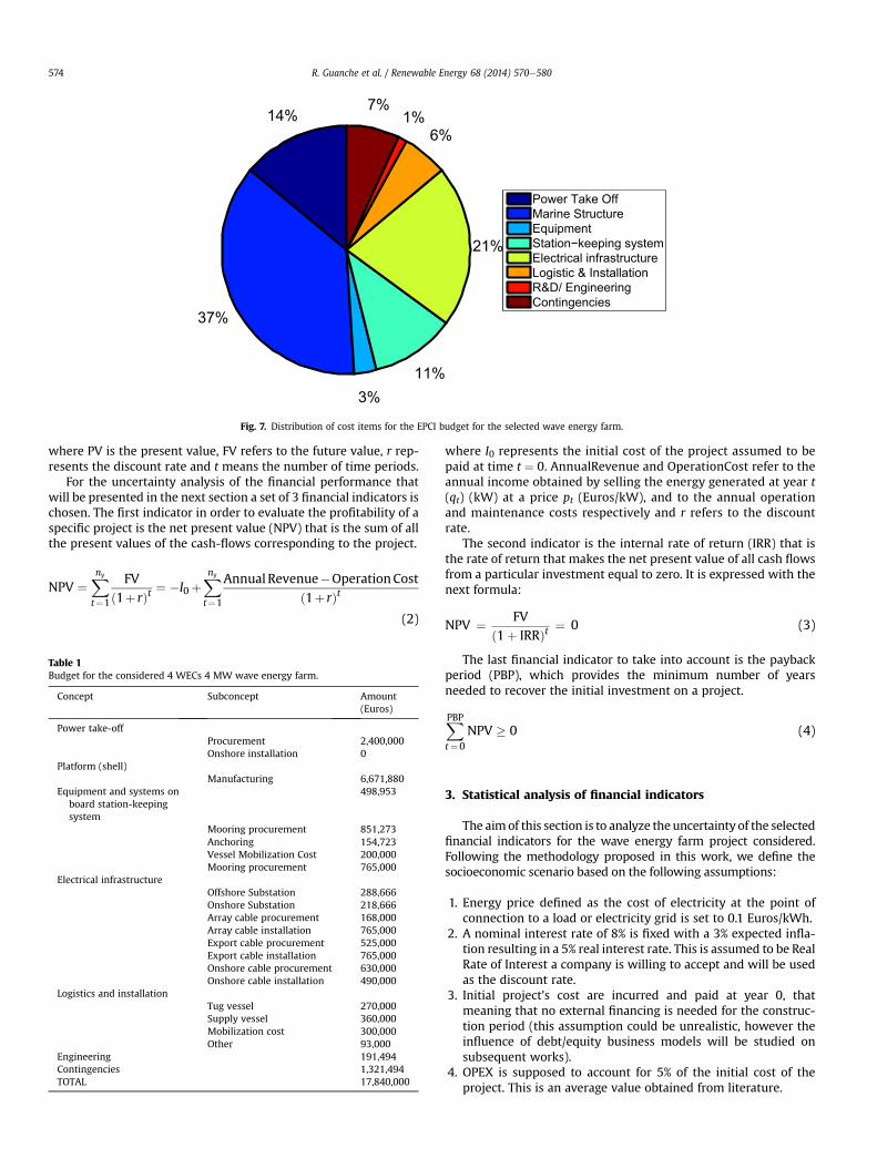
In this subsection, a brief description of the theoretical assump-tions and the estimates the parameters needed for the economicanalysis is given. First, the Engineering, Procurement, Constructionand Installation (EPCI) budget of the wave farm is presented inTable 1. The WEC is assumed to be built of steel and a concreteballast. Steel price is fixed at 5 Euros/kg. For concrete a cost of98.35 Euros/m3 is assumed. The cost of the linear generator is set to600.000 Euros/MW (personal communication to Dr. Guanche). Thislast assumption is an important source of uncertainty due to the lackof experience in this field and the limited availability of commercialPTOs for this type of devices in themarket. This cost is selected basedon the state of the art of the generators in existingWEC prototypes ordemonstration projects. The prices of the logistics and installationand electrical infrastructure are based on a personal communicationto Dr. Guanche. For this calculation the wave farm of 4 devices isconsidered. The weight of the structure is 293,320 kg of steel (for theshell) and 2200 m3 of concrete for the ballast. As stated before it isassumed that the export cable length is 4.3 km, the array cabledistance is 16 km and the onshore cable length is 1 km.

As shown in Table 1 the budget of the project is quite high. Thepercentage of steel is nearly 37%, representing an important stakeof the cost. It would be possible to assume that for WECs that havebeen through several optimization phases this percentage could bereduced.

In order to complete the economic analysis, operating expenses(OPEX) have to be added. OPEX refers to the operation and main-tenance costs also taking into account the insurance cost. OPEXassessment is a difficult task due to the absence of experience in theoperation and maintenance of these devices. In order to provide avalue a review of the existing percentages with respect to the initialcost of the project is carried out. Ref. [8] presented a table compilingOPEX costs in available projects suggesting values ranging between1.4% and 7% of the total project initial cost. In this study an averagevalue of 5% is taken based on a conservative approach. A totalreplacement of the devices is proposed at themiddle of the life-cycle.A conservative value has been assumed due to the lack of experienceregarding the durability of these types of structures at sea.

No project financing is considered and payment of the initialcost of the project is set at year 0 in the cash-flow analysis as it isconventionally assumed in project financing studies (f.i [19]). Thisassumption is also assumed on Ref. [8]. It is known that thisassumption is probably unrealistic, however on this study theinfluence of other factors is highlighted and the influence of thedebt/equity financing will be studied on future studies.

2.6. Discounted cash-flow algorithm

The discounted cash flow technique is a method assessing thevalue of a project, company or asset by measuring the expectedfuture cash flows derived from its operation, introducing the timevalue of money to capture the opportunity cost of the money tied upin the project. All future cash flows are estimated and discounted togive their present values (PVs). The sum of all future cash flows, bothincoming and outgoing, is the present value of the project (PV),which summarizes in a single value the overall distribution of cashflows derived from the project. The future value, FV, of a series ofcash flows refers to the future value, at future time n (total periods inthe future), of the sum of the future values of all cash flows, CF.

The cash flow analysis is based on the following formula:

PV ¼ FVð1þ rÞt (1)

14%

37%

3%11%

21%

6%1%

7%

Power Take OffMarine StructureEquipmentStation−keeping systemElectrical infrastructureLogistic & InstallationR&D/ EngineeringContingencies

Fig. 7. Distribution of cost items for the EPCI budget for the selected wave energy farm.

R. Guanche et al. / Renewable Energy 68 (2014) 570e580574

where PV is the present value, FV refers to the future value, r rep-resents the discount rate and t means the number of time periods.

For the uncertainty analysis of the financial performance thatwill be presented in the next section a set of 3 financial indicators ischosen. The first indicator in order to evaluate the profitability of aspecific project is the net present value (NPV) that is the sum of allthe present values of the cash-flows corresponding to the project.

NPV ¼Xny

t¼1

FVð1þ rÞt ¼ �I0þ

Xny

t¼1

Annual Revenue�OperationCostð1þ rÞt

(2)

Table 1Budget for the considered 4 WECs 4 MW wave energy farm.

Concept Subconcept Amount(Euros)

Power take-offProcurement 2,400,000Onshore installation 0

Platform (shell)Manufacturing 6,671,880

Equipment and systems onboard station-keepingsystem

498,953

Mooring procurement 851,273Anchoring 154,723Vessel Mobilization Cost 200,000Mooring procurement 765,000

Electrical infrastructureOffshore Substation 288,666Onshore Substation 218,666Array cable procurement 168,000Array cable installation 765,000Export cable procurement 525,000Export cable installation 765,000Onshore cable procurement 630,000Onshore cable installation 490,000

Logistics and installationTug vessel 270,000Supply vessel 360,000Mobilization cost 300,000Other 93,000

Engineering 191,494Contingencies 1,321,494TOTAL 17,840,000

where I0 represents the initial cost of the project assumed to bepaid at time t ¼ 0. AnnualRevenue and OperationCost refer to theannual income obtained by selling the energy generated at year t(qt) (kW) at a price pt (Euros/kW), and to the annual operationand maintenance costs respectively and r refers to the discountrate.

The second indicator is the internal rate of return (IRR) that isthe rate of return that makes the net present value of all cash flowsfrom a particular investment equal to zero. It is expressed with thenext formula:

NPV ¼ FVð1þ IRRÞt ¼ 0 (3)

The last financial indicator to take into account is the paybackperiod (PBP), which provides the minimum number of yearsneeded to recover the initial investment on a project.

XPBP

t¼0

NPV � 0 (4)

3. Statistical analysis of financial indicators

The aimof this section is to analyze the uncertainty of the selectedfinancial indicators for the wave energy farm project considered.Following the methodology proposed in this work, we define thesocioeconomic scenario based on the following assumptions:

1. Energy price defined as the cost of electricity at the point ofconnection to a load or electricity grid is set to 0.1 Euros/kWh.

2. A nominal interest rate of 8% is fixed with a 3% expected infla-tion resulting in a 5% real interest rate. This is assumed to be RealRate of Interest a company is willing to accept and will be usedas the discount rate.

3. Initial project’s cost are incurred and paid at year 0, thatmeaning that no external financing is needed for the construc-tion period (this assumption could be unrealistic, however theinfluence of debt/equity business models will be studied onsubsequent works).

4. OPEX is supposed to account for 5% of the initial cost of theproject. This is an average value obtained from literature.

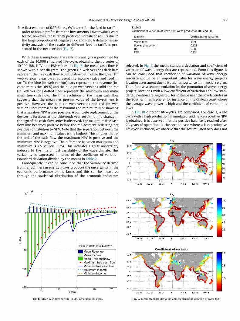
Table 2Coefficient of variation of wave flux, wave production IRR and PBP.

Element Coefficient of variation

Wave flux 1.39Power production 0.128IRR 0.08PBP 0.12

R. Guanche et al. / Renewable Energy 68 (2014) 570e580 575

5. A first estimate of 0.55 Euros/kWh is set for the feed in tariff inorder to obtain profits from the investments. Lower values weretested, however, these tariffs produced unrealistic results due tothe large proportion of negative IRR and PBP. A detailed sensi-tivity analysis of the results to different feed in tariffs is pre-sented in the next section (Fig. 7).

With these assumptions, the cash flow analysis is performed foreach of the 10.000 simulated life-cycle, obtaining then a series of10.000 IRR, NPV and PBP values. In Fig. 8 the mean cash flow isshown with a bar diagram. The green (in web version) dark barsrepresent the free cash flow accumulative path while the green (inweb version) clear bars represent the income (sales and feed intariff); the blue (in web version) bars represents the revenue (In-come minus the OPEX) and the blue (in web version) solid and red(in web version) dotted lines represent the maximum and mini-mum free cash flow. The time evolution of the mean cash flowsuggests that the mean net present value of the investment ispositive. However, the blue (in web version) and red (in webversion) lines represent the maximum and minimum NPV showingthat a negative NPV is also possible. A complete replacement of thedevices is foreseen at the thirteenth year resulting in a change inthe sign of the cash-flow series is observed. Themaximum free cashflow line becomes positive before the replacement reflecting netpositive contribution to NPV. Note that the separation between theminimum and maximum values is the highest. This implies that atthe end of the cash flow the maximum NPV is positive and theminimum NPV is negative. The difference between maximum andminimum is 2.5 Million Euros. This indicates a great uncertaintyinduced by the interannual variability of the wave climate. Thisvariability is expressed in terms of the coefficient of variation(standard deviation divided by the mean) in Table 2.

Consequently, it can be concluded that the variability derivedfrom randomness in energy fluxes produces the uncertainty in theeconomic performance of the farms and this can be measuredthrough the statistical distribution of the economic indicators

5 10 15 20 25−20

−15

−10

−5

0

5 x 106

Years

Eur

os

Feed in tariff= 0.55 Eur/kWh

Mean RevenueMean IncomeMean Free cashflowMaximum free cash flowMinimum free cashflowMaximum incomeMinimum income

Fig. 8. Mean cash-flow for the 10,000 generated life-cycle.

selected. In Fig. 9 the mean, standard deviation and coefficient ofvariation of wave energy flux are represented. From this figure, itcan be concluded that coefficient of variation of wave energyresource should be an important value for wave energy projectslocation assessment due to its high importance in financial returns.Therefore, as a recommendation for the promotion of wave energyproject, locations with a low coefficient of variation and low stan-dard deviation are suggested, for instance near the low latitudes inthe Southern hemisphere (for instance on the Chilean coast wherethe average wave power is high and the coefficient of variation islow).

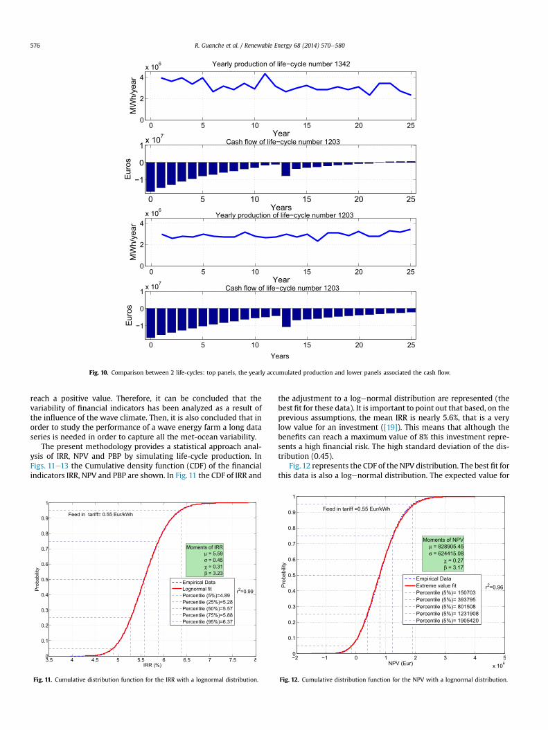
In Fig. 10 different life-cycles are compared. For case 1, a lifecycle with a high production is simulated, and hence a positive NPVis obtained. It is observed that the positive balance is reached after22 years of operation. In the second case where a less productivelife-cycle is chosen, we observe that the accumulated NPV does not

Fig. 9. Mean, standard deviation and coefficient of variation of wave flux.

0 5 10 15 20 250

2

4x 106 Yearly production of life−cycle number 1342

YearM

Wh/

year

0 5 10 15 20 25

−1

0

1x 107

Cash flow of life−cycle number 1203

Years

Eur

os

0 5 10 15 20 250

2

4x 106

Yearly production of life−cycle number 1203

Year

MW

h/ye

ar

0 5 10 15 20 25

−1

0

1x 107

Cash flow of life−cycle number 1203

Years

Eur

os

Fig. 10. Comparison between 2 life-cycles: top panels, the yearly accumulated production and lower panels associated the cash flow.

R. Guanche et al. / Renewable Energy 68 (2014) 570e580576

reach a positive value. Therefore, it can be concluded that thevariability of financial indicators has been analyzed as a result ofthe influence of the wave climate. Then, it is also concluded that inorder to study the performance of a wave energy farm a long dataseries is needed in order to capture all the met-ocean variability.

The present methodology provides a statistical approach anal-ysis of IRR, NPV and PBP by simulating life-cycle production. InFigs. 11e13 the Cumulative density function (CDF) of the financialindicators IRR, NPV and PBP are shown. In Fig. 11 the CDF of IRR and

Fig. 11. Cumulative distribution function for the IRR with a lognormal distribution.

the adjustment to a logenormal distribution are represented (thebest fit for these data). It is important to point out that based, on theprevious assumptions, the mean IRR is nearly 5.6%, that is a verylow value for an investment ([19]). This means that although thebenefits can reach a maximum value of 8% this investment repre-sents a high financial risk. The high standard deviation of the dis-tribution (0.45).

Fig.12 represents the CDF of the NPV distribution. The best fit forthis data is also a logenormal distribution. The expected value for

Fig. 12. Cumulative distribution function for the NPV with a lognormal distribution.

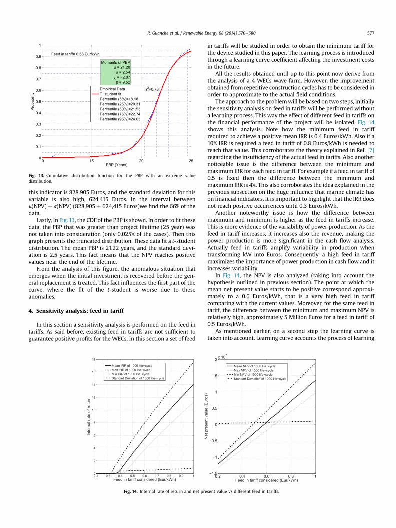
Fig. 13. Cumulative distribution function for the PBP with an extreme valuedistribution.

R. Guanche et al. / Renewable Energy 68 (2014) 570e580 577

this indicator is 828.905 Euros, and the standard deviation for thisvariable is also high, 624.415 Euros. In the interval betweenm(NPV) � s(NPV) (828,905 � 624,415 Euros)we find the 66% of thedata.

Lastly, In Fig. 13, the CDF of the PBP is shown. In order to fit thesedata, the PBP that was greater than project lifetime (25 year) wasnot taken into consideration (only 0.025% of the cases). Then thisgraph presents the truncated distribution. These data fit a t-studentdistribution. The mean PBP is 21.22 years, and the standard devi-ation is 2.5 years. This fact means that the NPV reaches positivevalues near the end of the lifetime.

From the analysis of this figure, the anomalous situation thatemerges when the initial investment is recovered before the gen-eral replacement is treated. This fact influences the first part of thecurve, where the fit of the t-student is worse due to theseanomalies.

4. Sensitivity analysis: feed in tariff

In this section a sensitivity analysis is performed on the feed intariffs. As said before, existing feed in tariffs are not sufficient toguarantee positive profits for the WECs. In this section a set of feed

0.2 0.3 0.4 0.5 0.6 0.7 0.8 0.9 10

2

4

6

8

10

12

14

16

18

Feed in tariff considered (Eur/kWh)

Inte

rnal

rate

of r

etur

n

Mean IRR of 1000 life−cycleMax IRR of 1000 life−cycleMin IRR of 1000 life−cycleStandart Deviation of 1000 life−cycle

Fig. 14. Internal rate of return and net pre

in tariffs will be studied in order to obtain the minimum tariff forthe device studied in this paper. The learning process is introducedthrough a learning curve coefficient affecting the investment costsin the future.

All the results obtained until up to this point now derive fromthe analysis of a 4 WECs wave farm. However, the improvementobtained from repetitive construction cycles has to be considered inorder to approximate to the actual field conditions.

The approach to the problemwill be based on two steps, initiallythe sensitivity analysis on feed in tariffs will be performed withouta learning process. This way the effect of different feed in tariffs onthe financial performance of the project will be isolated. Fig. 14shows this analysis. Note how the minimum feed in tariffrequired to achieve a positive mean IRR is 0.4 Euros/kWh. Also if a10% IRR is required a feed in tariff of 0.8 Euros/kWh is needed toreach that value. This corroborates the theory explained in Ref. [7]regarding the insufficiency of the actual feed in tariffs. Also anothernoticeable issue is the difference between the minimum andmaximum IRR for each feed in tariff. For example if a feed in tariff of0.5 is fixed then the difference between the minimum andmaximum IRR is 4%. This also corroborates the idea explained in theprevious subsection on the huge influence that marine climate hason financial indicators. It is important to highlight that the IRR doesnot reach positive occurrences until 0.3 Euros/kWh.

Another noteworthy issue is how the difference betweenmaximum and minimum is higher as the feed in tariffs increase.This is more evidence of the variability of power production. As thefeed in tariff increases, it increases also the revenue, making thepower production is more significant in the cash flow analysis.Actually feed in tariffs amplify variability in production whentransforming kW into Euros. Consequently, a high feed in tariffmaximizes the importance of power production in cash flow and itincreases variability.

In Fig. 14, the NPV is also analyzed (taking into account thehypothesis outlined in previous section). The point at which themean net present value starts to be positive correspond approxi-mately to a 0.6 Euros/kWh, that is a very high feed in tariffcomparing with the current values. Moreover, for the same feed intariff, the difference between the minimum and maximum NPV isrelatively high, approximately 5 Million Euros for a feed in tariff of0.5 Euros/kWh.

As mentioned earlier, on a second step the learning curve istaken into account. Learning curve accounts the process of learning

0.2 0.4 0.6 0.8 1−1.5

−1

−0.5

0

0.5

1

1.5

2 x 107

Feed in tariff considered (Eur/kWh)

Net

pre

sent

val

ue (E

uros

)

Mean NPV of 1000 life−cycleMax NPV of 1000 life−cycleMin NPV of 1000 life−cycleStandart Deviation of 1000 life−cycle

sent value vs different feed in tariffs.

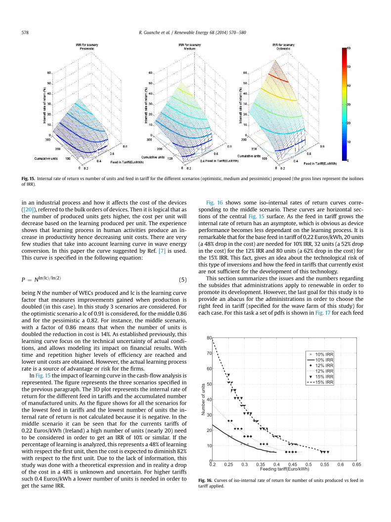
Fig. 15. Internal rate of return vs number of units and feed in tariff for the different scenarios (optimistic, medium and pessimistic) proposed (the gross lines represent the isolinesof IRR).

0.2 0.25 0.3 0.35 0.4 0.45 0.5 0.55 0.6 0.650

10

20

30

40

50

60

70

80

Num

ber o

f uni

ts

Feeding tariff(Euro/kWh)

10% IRR10% IRR12% IRR12% IRR15% IRR15% IRR

Fig. 16. Curves of iso-internal rate of return for number of units produced vs feed intariff applied.

R. Guanche et al. / Renewable Energy 68 (2014) 570e580578

in an industrial process and how it affects the cost of the devices([20]), referred to the bulk orders of devices. Then it is logical that asthe number of produced units gets higher, the cost per unit willdecrease based on the learning produced per unit. The experienceshows that learning process in human activities produce an in-crease in productivity hence decreasing unit costs. There are veryfew studies that take into account learning curve in wave energyconversion. In this paper the curve suggested by Ref. [7] is used.This curve is specified in the following equation:

P ¼ NlnðlcÞ=lnð2Þ (5)

being N the number of WECs produced and lc is the learning curvefactor that measures improvements gained when production isdoubled (in this case). In this study 3 scenarios are considered. Forthe optimistic scenario a lc of 0.91 is considered, for themiddle 0.86and for the pessimistic a 0.82. For instance, the middle scenario,with a factor of 0.86 means that when the number of units isdoubled the reduction in cost is 14%. As established previously, thislearning curve focus on the technical uncertainty of actual condi-tions, and allows modeling its impact on financial results. Withtime and repetition higher levels of efficiency are reached andlower unit costs are obtained. However, the actual learning processrate is a source of advantage or risk for the firms.

In Fig.15 the impact of learning curve in the cash-flowanalysis isrepresented. The figure represents the three scenarios specified inthe previous paragraph. The 3D plot represents the internal rate ofreturn for the different feed in tariffs and the accumulated numberof manufactured units. As the figure shows for all the scenarios forthe lowest feed in tariffs and the lowest number of units the in-ternal rate of return is not calculated because it is negative. In themiddle scenario it can be seen that for the currents tariffs of0.22 Euros/kWh (Ireland) a high number of units (nearly 20) needto be considered in order to get an IRR of 10% or similar. If thepercentage of learning is analyzed, this represents a 48% of learningwith respect the first unit, then the cost is expected to diminish 82%with respect to the first unit. Due to the lack of information, thisstudy was done with a theoretical expression and in reality a dropof the cost in a 48% is unknown and uncertain. For higher tariffssuch 0.4 Euros/kWh a lower number of units is needed in order toget the same IRR.

Fig. 16 shows some iso-internal rates of return curves corre-sponding to the middle scenario. These curves are horizontal sec-tions of the central Fig. 15 surface. As the feed in tariff grows theinternal rate of return has an asymptote, which is obvious as deviceperformance becomes less dependant on the learning process. It isremarkable that for the base feed in tariff of 0,22 Euros/kWh, 20 units(a 48% drop in the cost) are needed for 10% IRR, 32 units (a 52% dropin the cost) for the 12% IRR and 80 units (a 62% drop in the cost) forthe 15% IRR. This fact, gives an idea about the technological risk ofthis type of inversions and how the feed in tariffs that currently existare not sufficient for the development of this technology.

This section summarizes the issues and the numbers regardingthe subsides that administrations apply to renewable in order topromote its development. However, the last goal for this study is toprovide an abacus for the administrations in order to choose theright feed in tariff (specified for the wave farm of this study) foreach case. For this task a set of pdfs is shown in Fig. 17 for each feed

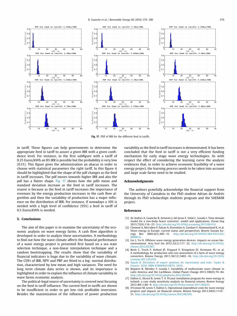
Fig. 17. PDF of IRR for the different feed in tariffs.

R. Guanche et al. / Renewable Energy 68 (2014) 570e580 579

in tariff. These figures can help governments to determine theappropriate feed in tariff to assure a given IRR with a given confi-dence level. For instance, in the first subfigure with a tariff of0.25 Euros/kWh an 8% IRR is possible but the probability is very low(0.1%). This figure gives the administration an abacus in order tochoose with statistical parameters the right tariff. In this figure itshould be highlighted that the shape of the pdf changes as the feedin tariff increases. The pdf moves towards higher IRR and also thepdf has a flatter shape. Fig. 17 shows how the pdfs mean andstandard deviation increase as the feed in tariff increases. Thereason is because as the feed in tariff increases the importance ofrevenues by the energy production increases in the cash flow al-gorithm and then the variability of production has a major influ-ence on the distribution of IRR. For instance, if nowadays a 10% isneeded with a high level of confidence (95%) a feed in tariff of0.5 Euros/kWh is needed.

5. Conclusions

The aim of this paper is to examine the uncertainty of the eco-nomic analysis on wave energy farms. A cash flow algorithm isdeveloped in order to analyze these uncertainties. A methodologyto find out how the wave climate affects the financial performanceof a wave energy project is presented first based on a sea stateselection technique, a non-linear interpolation technique and arandom bootstrapping. The results show that the variability offinancial indicators is huge due to the variability of wave climate.The CDFs of IRR, NPV and PBP are fitted to a logenormal distribu-tion, characterized by low mean and high variances. The need forlong term climate data series is shown, and its importance ishighlighted in order to explain the influence of climate variability inwave farms economic analysis.

The political-legal source of uncertainty is covered next focusingon the feed in tariff influence. The current feed in tariffs are shownto be insufficient in order to get low risk profitable inversions.Besides the maximization of the influence of power production

variability as the feed in tariff increases is demonstrated. It has beenconcluded that the feed in tariff is not a very efficient fundingmechanism for early stage wave energy technologies. As withrespect the effect of considering the learning curve the analysisevidences that, in order to achieve economic feasibility of a waveenergy project, the learning process needs to be taken into accountand large scale farms need to be studied.

Acknowledgments

The authors gratefully acknowledge the financial support fromthe University of Cantabria to the PhD student Adrian de Andrésthrough its PhD scholarships students program and the SAEMARproject.

References

[1] de Andres A, Guanche R, Armesto J, del Jesus F, Vidal C, Losada I. Time domainmodel for a two-body heave converter: model and applications. Ocean Eng2013;72(0):116e23. http://dx.doi.org/10.1016/j.oceaneng.2013.06.019.

[2] Clement A, McCullen P, Falcao A, Fiorentino A, Gardner F, Hammarlund K, et al.Wave energy in Europe: current status and perspectives. Renew Sustain En-ergy Rev 2002;6(5):405e31. http://dx.doi.org/10.1016/S1364-0321(02)00009-6.

[3] Lin L, Yu H. Offshore wave energy generation devices: impacts on ocean bio-environment. Acta Ecol Sin 2012;32(3):117e22. http://dx.doi.org/10.1016/j.chnaes.2012.02.007.

[4] Beels C, Troch P, Kofoed JP, Frigaard P, Kringelum JV, Kromann PC, et al.A methodology for production and cost assessment of a farm of wave energyconverters. Renew Energy 2011;36(12):3402e16. http://dx.doi.org/10.1016/j.renene.2011.05.019.

[5] Ayyub B. Elicitation of expert opinions for uncertainty and risks. Taylor &Francis; 2010, ISBN 9780849310874; 2010.

[6] Reguero B, Mendez F, Losada I. Variability of multivariate wave climate inLatin America and the Caribbean. Global Planet Change 2013;100(0):70e84.http://dx.doi.org/10.1016/j.gloplacha.2012.09.005.

[7] Dalton G, Alcorn R, Lewis T. A 10 year installation program for wave energy inIreland: a case study sensitivity analysis on financial returns. Renew Energy2012;40(1):80e9. http://dx.doi.org/10.1016/j.renene.2011.09.025.

[8] O’Connor M, Lewis T, Dalton G. Operational expenditure costs for wave energyprojects and impacts on financial returns. Renew Energy 2013;50(0):1119e31. http://dx.doi.org/10.1016/j.renene.2012.08.059.

R. Guanche et al. / Renewable Energy 68 (2014) 570e580580

[9] O’Connor M, Lewis T, Dalton G. Techno-economic performance of the Pelamisp1 and wavestar at different ratings and various locations in Europe. RenewEnergy 2013;50(0):889e900. http://dx.doi.org/10.1016/j.renene.2012.08.009.

[10] Babarit A, Hals J, Muliawan M, Kurniawan A, Moan T, Krokstad J. Numericalbenchmarking study of a selection of wave energy converters. Renew Energy2012;41(0):44e63. http://dx.doi.org/10.1016/j.renene.2011.10.002.

[11] IHCantabria. ENOLA project. URL, http://www.enola.ihcantabria.com/; 2011.[12] Hernndez-Brito J, Monagas V, Gonzlez J, Schallenberg J, Llins O. Vision for

marine renewables in the canary islands. In: 4th International Conference onOcean Energy, 17 October, Dublin; 2012.

[13] Reguero B, Menndez M, Mndez F, Mnguez R, Losada I. A global ocean wave(GOW) calibrated reanalysis from 1948 onwards. Coast Eng 2012;65(0):38e55. http://dx.doi.org/10.1016/j.coastaleng.2012.03.003.

[14] Camus P, Mendez FJ, Medina R. A hybrid efficient method to downscale waveclimate to coastal areas. Coast Eng 2011;58(9):851e62. http://dx.doi.org/10.1016/j.coastaleng.2011.05.007.

[15] DNV. SESAM users manual. WADAM; 2008. URL, http://www.dnv.cl/services/software/products/sesam/sesamhydrod/wadam.asp.

[16] de Andres A, Guanche R, Meneses L, Vidal C, Losada IJ. Factors that influencearray layout on wave energy farms [submitted for publication] Ocean Eng;2013.

[17] Espejo A, Minguez R, Tomas A, Menendez M, Mendez F, Losada I. Directionalcalibrated wind and wave reanalysis databases using instrumental data foroptimal design of off-shore wind farms. In: OCEANS, 2011 IEEE e Spain; 2011.pp. 1e9. http://dx.doi.org/10.1109/Oceans-Spain.2011.6003592.

[18] Harris RE, Johanning L, Wolfram J. Mooring systems for wave energy con-verters: a review of design issues and choices. In: 3rd International Confer-ence on Marine Renewable Energy, Blyth, UK; 2004.

[19] Donald G, Newnan P, Lavelle J. Essentials of engineering economic analysis.Engineering Press; 1998, ISBN 9781576450284; 1998.

[20] Wright TP. Factors affecting the cost of airplanes. J Aeronaut Sci 1936;3:122e8.