unbalanced government budgets, private asset holdings, and the traditional comparative static...

HARLAND WM. WHITMORE, JR. University of Cincinnati

Unbalanced Government Budgets, Private Asset Holdings, and the Traditional Comparative Static Multipliers *

During the past quarter century, the traditional macro model of effective demand has been criticized repeatedly for ignoring certain asset market effects associated with government policy. The customary approach in using an underlying framework for this model has been to assume that government faces a budget constraint whereas the private sector confronts a wealth constraint. In this paper, we demonstrate that if every sector faces a budget constraint, many of the aforementioned criticisms disappear. One particularly interesting result is that a balanced government budget is not necessary to achieve a stationary equilibrium for national income.

1. Introduction Depending upon which interpretation of “timelessness” we

adopt, a given intersection of IS and LM in the simple static textbook model of aggregate demand can refer to general equilibrium levels of national income and the interest rate either for a particular moment in time with ties neither to the past nor future, or to a “stationary state” in which these variables remain constant over time. Analo- gously, the standard comparative static policy multipliers attached to this model can conceivably represent either initial impacts only, or total changes in the stationary state levels of these variables. Of course, under the latter interpretation, unless net investment equals zero at such a solution, an IS-LM stationary state necessarily ignores the effects of changes in physical capital upon factor products and their subsequent impacts upon the economy. In this sense, the so-called stationary state merely represents “short-period equilibrium” [see Allen (1967), p. 761.

During the last twenty-five years, however, a growing number of authors have criticized the second interpretation of an IS-LM

*The author wishes to thank Professors Carl Christ and Jerome Stein for helpful comments on an earlier draft of this paper.

Journal of Macroeconomics, Spring 1980, Vol. 2, No. 2, pp. 129-157 129 @ Wayne State University Press, 1980.

Harland Wm. Whitmore, 3~.

equilibrium and the standard policy multipliers on the grounds that they also ignore changes in private sector asset holdings generated by monetary and fiscal actions. Ritter (1956) and Pesek and Saving (1968), for instance, argue that a combined once-for-all shift to the right in IS and LM commonly associated with a “money financed” rise in government spending is incomplete because it ignores all increments to the money supply except the initial one. Christ (1968 and 1978) claims that the standard comparative static multipliers are incorrect in general because (a) they necessarily abstract from the government’s budget constraint-which he regards as an inherently dynamic concept;’ and (b) they ignore changes in private asset holdings associated with government deficits and surpluses. Disallowing government bonds, Christ (1968) finds a balanced budget is necessary to achieve a stationary solution for national income once the budget constraint is introduced. Hence a positive marginal tax rate is necessary to reach a new stationary state, following an unbalanced rise in government spending financed initially by printing money. Allowing for government borrowing, Christ (1978) finds a balanced budget is no longer necessary to achieve a stationary solution for real national income if commodity prices are variable. However, he claims real money balances and real government bonds outstanding must remain fixed at a stationary solution for real national income. Consequently, if the (exogenously determined) inflation rate is set equal to zero, nominal money and government bonds outstanding must also remain unchanged. Once again, a balanced budget is required to achieve constant real income.

Silber (1970) and Meyer (1975) assert that even after appending the government’s budget constraint to the conventional IS-LM equations, the standard model continues to disregard the effects of changes in bond supply generated by debt financed increases in government spending unless wealth effects appear in the consumption and demand for money functions.’ With these wealth effects present, they argue, an entirely bond-financed permanent rise in government spending may cause national income to fall

‘In his 1978 paper Christ argues that this constraint is static or dynamic depending upon which policy variables we select as exogenous. We will return to this matter at a later point.

*Like all the others, Silber argues that the simple IS-LM model also “ignores the impact of net investment upon the stock of capital” [(1970), p. 4631. As we will show however, it is possible to view the standard model as incorporating the effects of net private investment upon the stock of capial, at least insofar as the asset holdings of the private sector are concerned.

130

Unbalanced Government Budgets

below its original level after n periods. According to Blinder and Solow (1973 and 1976b), if government interest payments are also explicitly introduced into the analysis, the situation is reversed. Not only ‘does a permanent bond-financed increase in government spending raise national income, but, contrary to the conventional result, this type of financing becomes even more expansionary than the “money financed” case. Also under their assumptions, an open market purchase contracts national income. Now it is the standard comparative static multiplier attached to a pure monetary action which appears to exhibit the wrong sign.

The balanced portfolio hypothesis developed by Metzler (1951) and extended by Tobin (1969) plays an implicit role in the papers by Christ (1968 and 1978) and Silber (1970). A wealth constraint imposed upon the private sector provides a basis for this hypothesis by imposing the restriction that the level of net wealth attached to the desired balance sheet must be identically equal to existing private net wealth. Under the wealth constraint, the various demands for assets and ex ante supplies of liabilities represent a desired arrangement of existing net wealth.

Following Patinkin (1965) and May (1970), Turnovsky (1977a and 1977b) advocates subjecting not only the government but also the household and business sectors to a budget constraint.3 It stipulates that a sector’s plans for net accumulations of specific assets and/or net retirements of specific liabilities during the period must be consistent with ex ante net saving during the period on the income account. Given net wealth at the beginning of the period, the asset demands and ex ante supplies appearing in this constraint represent planned amounts for the end of the period. Since no distinction is made between the existing amounts of specific assets and liabilities on the one hand and their desired beginning of period levels on the other, the budget constraint clearly abstracts from “current portfolio imbalance” and concentrates instead upon the asset market decisions associated with the decision to save.

My purpose in this paper is to show that if we view every sector in the simple IS-LM framework as subject to a budget constraint, then, except for the aforementioned exclusion of the impact of net investment upon factor products, the standard comparative static multipliers are indeed complete under the second

‘Turnovsky (1977a), May (1970), and Turnovsky and Burmeister (1977) agree that in the limit the latter constraints (but not the government’s) reduce to wealth constraints. Later we will return to this point.

131

Harland Wm. Whitmore, Jr.

interpretation outlined earlier. In particular, the combined once- for-all shift in IS and LM commonly associated with a money financed rise in government spending is complete in that it depicts the total changes in the stationary levels of national income and the interest rate induced by a permanent increase in government spending which is bond financed in every period except the first-when the printing press is used. Also, the three standard comparative static policy multipliers which Christ labels as “ignoring the government’s budget constraint” represent changes in stationary levels of national income that result from government actions involving alterations in the level of outstanding government debt-a possibility not considered in his 1968 paper. Also, under the budget constraint approach, the standard comparative static policy multipliers do indeed incorporate the effects of changes in bond supply even without wealth effects appearing in the consumption and demand for money functions. Furthermore, if the system is stable, the introduction of wealth effects into these functions alters the magnitudes of the policy multipliers but not their signs; Silber’s (1970) assertion to the contrary notwithstanding, a bond-financed increase in government spending continues to expand national income.

Following Turnovsky, we assume firms neither hold money balances at the beginning of any period nor plan to hold money at the end of any period. Because households therefore represent the only sector demanding money, personal income becomes the relevant variable in the demand for money function. Under these assumptions, the explicit introduction of government interest payments and the reformulation of the analysis in continuous time to conform to Blinder and Solow’s approach fail to undermine conventional results. Contrary to their findings, a rise in government spending financed initially by printing more money but financed continuously thereafter through the bond market is more expansionary than a purely bond-financed increase. Moreover, an open market purchase expands national income.

These conclusions rest heavily upon the fact that under the budget constraint approach advocated by Turnovsky and others, a balanced government budget is not necessary to achieve a stationary solution for national income and the interest rate if the price level is constant. As Hansen (1970) has shown, without wealth effects in the consumption or demand for money functions the wealth coefficient in the households’ demand for bonds is unity.

132


Consequently, if government expenditures, taxes, money supply, and the first difference of the government’s supply of real bonds remain fixed, a stationary state is possible in which households are just willing to apply their personal saving each period to acquire new bonds issued both by firms to finance net investment and by government to finance its deficit. The bond market demand and supply functions will both shift in the same direction by the same amount each period, thereby maintaining a constant equilibrium interest rate.

If wealth effects appear in the consumption and demand for money functions, net personal saving must equal zero at a stationary solution. If net private investment is to remain positive in a closed economy with zero net business saving, the government must continue to run a surplus every period. Assuming a fixed number of nontransferable equity shares outstanding which, following Turnovsky [(1977b), p. 371, the households value as equal to the difference in value between corporate assets (consisting only of physical capital) and corporate bonds outstanding, firms must finance net investment by additional borrowing. Under these conditions and given constant capital and bond prices, private net investment has no net effect upon the value of the outstanding equity shares. Households recognize that corporate assets and liabilities both increase every period by an amount equal to the fixed rate of net investment. Therefore, at a stationary solution, household money balances and equity share values remain unchanged. If the government uses its surplus to retire its own debt, households merely trade government bonds for an equivalent amount of corporate bonds, which they presumably regard as perfect substitutes. If, instead, the government buys corporate bonds, then even the composition of the household sector’s bond holdings remains unchanged.

Of course, the restriction that household wealth-consisting of money, bonds, and equity shares-remains constant at a stationary solution for national income does not preclude household wealth accumulation or contraction with changes in equilibrium income. As will be shown later, even though it eventually crowds out an equivalent amount of net private investment in the simple textbook IS-LM model, a permanent increase in government spending financed each period by a reduction in the rate of debt retirement raises the stationary-state levels of national income, personal consumption, and household wealth.

133


2. The Discrete Version of.lS-LM Including Budget Constraints According to each sector’s budget constraint, the net value

of the particular assets it plans to purchase during the period minus the net value of the particular liabilities it plans to sell must be identically equal to the amount it plans to save (net) out of income received during the period. Admittedly-though this is not the case in the equations typifying the simple IS-LM model-expected future prices may influence the quantities of various assets and liabilities which the decision maker plans to hold or have outstanding by the end of the period. Also, by the time the end of the period actually arrives, prices may have indeed changed. Neverthe- less, the prices which are appropriate for valuing the quantities of assets and liabilities planned for the beginning and end of any period within a budget constraint are the prices which are expected to prevail during the period delimited by that constraint. Therefore, regardless of which factors influence the demands and ex ante supplies contained in it, the current period’s budget constraint should value all beginning- and end-of-period assets and liabilities in current prices since they are the ones which the sector must plan to pay (or receive) in the asset markets as it decides how to allocate current saving.

This specification differs from Turnovsky’s [(1977a), p. 41. For all intents and purposes, he values all assets and liabilities in terms of expected end-of-period prices. On the surface, our approach also differs from Foley’s (1975) since both current and expected end-of-period prices enter his budget constraint explicitly. However, substituting his identity (A)4

w(t) = fim(t)Md(t) + &(t)Kd(t) (A)

into his budget constraint (6) for @(At) and W(O)5

*(At) - W(0) = (Yd - Cd)At + [&(At) - pk(0)] Kd (At)

+ I&, (4 - P, F-VI Md (At) (6)

yields an alternative expression for his budget constraint as given by his equation (7):

“w(t) is expected nonhuman wealth at time t; M”(t) and Kd (t) represent the demands for money and capital at time t; and 6, (t) and 5, (t) represent the expected prices of money and capital at time t.

‘Yd = [Qc + P,Q, + P, . D] and Cd = the demand for consumption.

134


(Yd- Cd)At = p,(O) [K”(At) - Kd(0)J

+ P, (0) Wd (At) - MdKVl.

This last identity conforms exactly to our specification outlined earlier in that the assets in both the beginning- and end-of-period balance sheets are valued in terms of current market prices.’

Except for the budget constraints facing the household and business sectors and a provision for income taxes, the equations presented next essentially reproduce Silber’s model. The incorpora- tion of the household sector’s budget constraint into the analysis demonstrates the point, made by Turnovsky (1975), that beginning- of-period wealth is the relevant wealth variable to include in the consumption and asset demand functions for the end of the period. Consequently, we deviate from Silber’s specification also by lagging wealth one period in these functions.

Household Sector Since we view the households as holding a fixed number

of non-transferable equity shares, they may save only by accumulat- ing money or bonds. Identity (1) defines their budget constraint:

y, - T, = cf + (M,d - M:‘_,) + (B:’ - B:‘_,) ,

where Y, - T, represents disposable income; Cd represents ex ante personal consumption; Mf represents the demand for money for

‘Although we adopt Foley’s budget constraint concept as given by his identity (7), we cannot subscribe to the remainder of his end-of-period model. The reason is that his end-of-period asset demands, Md(At) and Kd(At), depend solely upon expected rates of return and expected future wealth, @(At), as defined by his identity A. Substituting his demand functions for these assets into identity A yields an expression for expected future wealth that depends only upon expected future asset prices and rates of return. Consequently, Kd (At) and M d (At), when written exclusively in terms of variables which the decision maker takes as exogenous, also depend only upon expected future asset prices and rates of return. Rewriting the demand functions solely in terms of the exogenous variables and substituting the new expressions into Foley:s equation (7) produces the following unacceptable consumption function:

cd=cx+++ W(O),

where Q and the unitary wealth coefficient represent dimensionally different constants than the unitary marginal propensity to consume.

135


end-of-period t; and B t represents the households’ demand for bonds for end-of-period t.

Using Silber’s notation, the consumption and demand for money functions appear as equations (2) and (3):

Cf = a + b (Y, - T,) + IL (MI’_, + B,d_,) ;

M:’ = h(M;i_, + B,d_,) + fY, - vt , (3)

where a, b, p, h, f, and 4 are positive constants. The demand for bonds function implied by equations (1) through (3) is presented as equation (4):

Bf = - a + (1 - b - f) Y, + (b - 1) T, + qr,

+ (1 - h - P) CM:‘_, + B:-J . , (4)

Assuming bonds (i.e., future goods) are normal goods, (1 - b - f) and (1 - h - p) are both positive.

Non-bank Business Sector Given that disposable income is defined as Y, - T,, where

Y, = national income and T, = personal taxes less government transfers and interest, net business saving must be identically equal to zero; all business receipts other than depreciation expenses are distributed to the households as personal income. The business sector’s budget constraint appears as identity (5):

Z:’ = B;, - BJt-, , (5)

where Z,” = ex ante net private investment and B;t = the firms’ ex ante supply of bonds. Identity (5) reflects our earlier assumptions that (a) the number of equity shares outstanding is fixed; and (b) firms do not plan to hold money balances at the end of any period (although intraperiod transactions involving money presumably are not precluded).

Letting E, represent the value of the fixed number of equity shares, we have E, = K, - B,, where K, = the (value of the) physical capital held by firms at time t, and B, = outstanding corporate debt at time t. Household wealth at any moment, W,, is therefore defined as W, = B, + M, + E,, where B, = the (value of the) bonds held by the households at time t. Letting Bgt represent

136


outstanding government debt at time t, we have B, = B, + BeI. Consequently, W, is identical to Silber’s definition of household wealth: M, + Bgl + K,. Unlike Silber, however, we view the household sector as recognizing that net investment by firms alters K. Therefore, we view the standard IS-LM framework as incorporating the effects of the changes in K upon household wealth even though-as a model of aggregate demand only-it does abstract from the effects of change in K upon factor products.

Again employing Silber’s notation, the standard investment function is given by

z:’ = d - e rt , (6)

where rt = the interest rate and d and e represent positive constants. Together, equations (5) and (6) imply the following corporate bond supply function:

B;t = d - e rr + B>*-, .

Government Sector Identity (8) depicts the government’s budget constraint:

T, = G:’ - (Bzt - B;,-,) - (M,” - M:-,) , 03)

where

T,=v++Y,, (9)

and where Gf = ex ante government expenditures; B:, = the government’s ex ante supply of bonds for end-of-period t; MS = its ex ante supply of money for end-of-period t; and where v and i4 are policy parameters for lump sum taxes (net of government transfers and interest) and pers.onal income tax rates, respectively. Of course, at most four of the variables among G’, MS, B “, , u, and v may be exogenously determined.

Market Equilibrium Conditions The equilibrium conditions for the commodity, money, and

bond markets are defined by equations (10) through (12) respectively:

Y, = Cf + I:‘+ G:‘; (10)

137


M;= M;; (11)

B:‘= B; + Bt ; (12)

Given identities (l), (S), and (8) and given the initial conditions Bt = B, + B, and Mz = M t, it follows that if any two of equations (10) through (12) are satisfied for all t, so is the third.

The central issues surrounding the discrete version of the standard IS-LM model are (a) whether the multipliers, which Christ claims ignore the government’s budget constraint, actually reflect policies involving changes in real government debt outstanding; (b) whether the standard comparative static multipliers ignore changes in real bonds (and capital) held by the private sector if wealth effects are excluded from the consumption and demand for money functions; and (c) whether an entirely bond-financed permanent rise in government spending may cause national income to fall below its original level after n periods. Since each of these issues concerns activity in the bond market, we will focus attention squarely upon that market. In particular, we will use money and bond market equilibrium conditions implied by the aforementioned specification to solve for stationary levels of national income and the interest rate. The multipliers we derive for changes between stationary levels will therefore depend directly upon activity in the bond market. Because the government’s budget constraint forms a part of the underlying structure, these multipliers will also incorporate the restrictions imposed by this constraint.

Zssue a In accordance with Christ (1968), we set h = i.r, = 0. Treating

equations (2), (6), and (10) as redundant, first substitute (9) for T, in (8), (4), and (1). Second, substitute (11) for Md into equation (3) and the new equation (4) obtained in the first step. Third, substitute the new equation (3), obtained in the second step, for rt in the new equation (4) obtained in that step and in equation (7). Fourth, substitute the new equations (4) and (7) obtained in step three and equation (8) for Bd, B;, and B:, respectively, in equation (12). Since (12) holds for all t, the final forms for Y and r become

(9 [l - b(1 - u)] + ef}Yt = 9(a + d) - qbu + eMT + 9G, ;(14)

138


{9[1-b(l-u)] +ef}r,=f(a+d)-bfv+fGl

- [l-b(l-u)] Mr. (15)

Importantly, it is sufficient that u, v, M”, and G remain fixed to achieve constant levels of Y and r over time. From (8), this implies only that the first difference of the government’s supply of real bonds must remain constant. Contrary to Christ’s (1968 and 1978) results, a balanced budget is not necessary to achieve a stationary- state solution for real income and the interest rate in the simple IS-LM framework even if commodity prices remain constant.

A permanent rise in G which, except for induced changes in income taxes, is entirely bond financed produces the following multiplier effect upon the stationary level of Y:

dY/dG = l/[l - b(1 - u) + (ef/q)] . (16)

This multiplier, which Christ claims ignores the government’s budget constraint, is the same as the standard comparative static multiplier attached to a once-for-all shift in IS along a fixed LM due to a rise in G.

An increase in lump-sum taxes which, except for an induced reduction in income taxes, is accompanied by governmental debt retirement yields the following multiplier:

dY/dv = -bl[l-b(l-u)+(efl9)1. (17)

This multiplier is the same as the standard comparative static multiplier attached to a once-for-all shift in IS along a fixed LM due to a rise in v.

An open market purchase by the government creates the multiplier effect

dY/dM”= (e/q)/[l - b(1 - u) + (ef/q)] . 08)

As induced income taxes increase, additional government debt is retired. This multiplier is the same as the standard comparative static multiplier attached to a once-for-all shift in LM along a fixed IS arising from an increase in M”. Christ’s assertion to the contrary notwithstanding, this multiplier also clearly incorporates the restrictions imposed by the government’s budget constraint.

139


The fact that these three comparative static multipliers do in fact incorporate the restrictions imposed by the government’s budget constraint calls into question Christ’s assertion that the latter is an inherently dynamic concept. Actually it is a simple matter to specify a purely static version of the government’s budget constraint (no matter which policy variables we select as exogenous) once we recognize that it is entirely appropriate to view an exogenously determined variable as simultaneously representing an ex ante variable. Consider (19), the static equation

G=T+(M”-M,)+(B”,-Bgo), (1%

where G represents ex ante government expenditure (and hence forms a part of aggregate demand); T represents the planned (and announced) level of lump-sum personal taxes less transfers; and M ”and B “, represent, respectively, the government’s ex ante supplies of fiat money and bonds; and M, and B, represent the existing amounts of these items held by the private sector.

To stipulate that G is exogenous is to state merely that the amount the government plans to spend is invariant with respect to all other variables in the model. Analogously, an exogenous money supply, M”, signifies merely that the amount of money the government plans to have outstanding is invariant with respect to all other variables under consideration. But whether exogenously determined or not, the ex ante variable, M”, represents something quite different from the ex post magnitude, M,, which depicts the initial existing stock of money outstanding. Introduction of the time element is not necessary to distinguish between these two money concepts.

Specifying the other structural equations in a purely static setting yields:

z = B; - B, ;

Z = d - er ;

B;= BfO+d-er;

2’ - 2’ = C + (Md- M,) + (Bd - B,) ;

(20)

(21)

(22)

(23)

(24) C=a+b(Y-T);

140


Md=fY-qr; (25)

Bd = (1 - b -f) Y + (b - 1) T + qr + (M, + B,) - a ; (26)

Md= MS; (27)

Y=C+Z+G; (28)

Bd=B;+B;. (29)

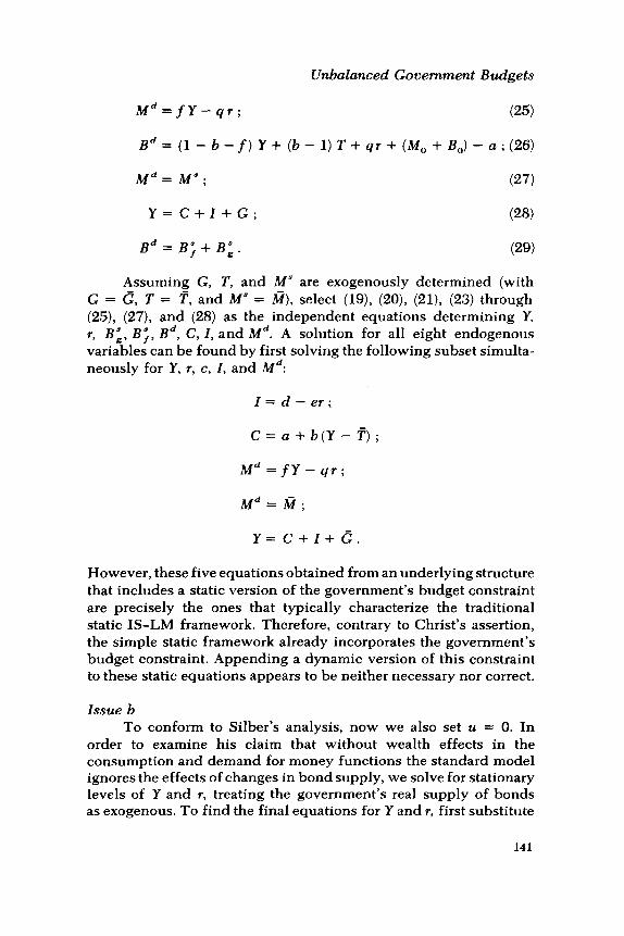
Assuming G, T, and M” are exogenously determined (with G = G, T = F, and MS = ri?), select (19), (20), (21), (23) through (25), (27), and (28) as the independent equations determining Y, r, Bi, B ;, Bd, C, I, and Md. A solution for all eight endogenous variables can be found by first solving the following subset simultaneously for Y, r, c, I, and Md:

Z = d - er ;

C=a+b(Y-7);

Md=fY-qr;

y=c+z+c.

However, these five equations obtained from an underlying structure that includes a static version of the government’s budget constraint are precisely the ones that typically characterize the traditional static IS-LM framework. Therefore, contrary to Christ’s assertion, the simple static framework already incorporates the government’s budget constraint. Appending a dynamic version of this constraint to these static equations appears to be neither necessary nor correct.

Issue b To conform to Silber’s analysis, now we also set u = 0. In

order to examine his claim that without wealth effects in the consumption and demand for money functions the standard model ignores the effects of changes in bond supply, we solve for stationary levels of Y and r, treating the government’s real supply of bonds as exogenous. To find the final equations for Y and r, first substitute

141


(9), with u = 0, for T, into equations (4) and (8). Second, substitute (8) for 0 in the new equation (4). Third, substitute (11) for Md in (3) and then substitute the new equation (3) for r into (7) and the new equation (4) obtained in step two. Fourth, recognizing that equation (12) implies that

substitute the new equations (4) and (7) obtained in step three for the first differences on the right-hand side of this respecification of (12):

[q (1 - b) + ef] Yt = 9 (a + d) + @9 + 4 MT - b9 MG1

+ WB”,, - B;,J + (1 - b) 9 G, ; (30)

‘[9 (1 - b) + efl r, = f(a + d) + (b + f b - 1) M: - bf Mr-,

+ bf (BL1 - B”,+,) + f (1 - b) G, . (31)

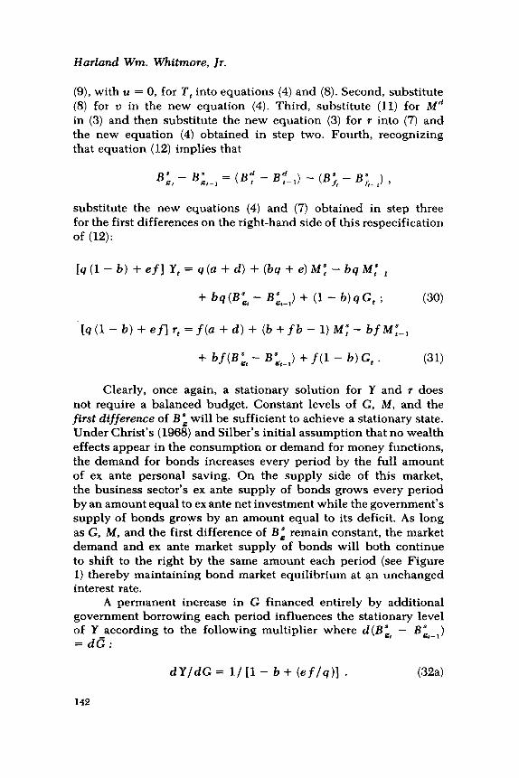
Clearly, once again, a stationary solution for Y and r does not require a balanced budget. Constant levels of G, M, and the first difference of B “, will be sufficient to achieve a stationary state. Under Christ’s (1968) and Silber’s initial assumption that no wealth effects appear in the consumption or demand for money functions, the demand for bonds increases every period by the full amount of ex ante personal saving. On the supply side of this market, the business sector’s ex ante supply of bonds grows every period by an amount equal to ex ante net investment while the government’s supply of bonds grows by an amount equal to its deficit. As long as G, M, and the first difference of Bi remain constant, the market demand and ex ante market supply of bonds will both continue to shift to the right by the same amount each period (see Figure 1) thereby maintaining bond market equilibrium at an unchanged interest rate.

A permanent increase in G financed entirely by additional government borrowing each period influences the stationary level of Y according to the following multiplier where d (B :, - B:,- ,) =dc:

dY/dG = l/ [l - b + (ef/q)] . (324

142


r

Figure 1.

Bonds

Since the coefficient of the first difference of the government’s real supply of bonds in (30) forms part of this multiplier, the latter definitely incorporates the effects of changes in bond supply attached to this pure fiscal policy. However, this is precisely the standard comparative static result associated with a permanent shift in IS along a fixed LM for a change in G.

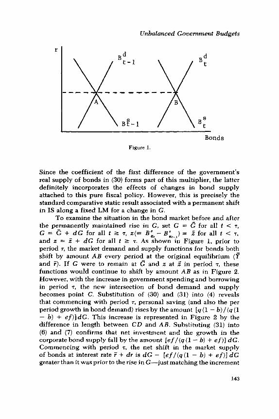
To examine the situation in the bond market before and after the permanently maintained rise in G, set G = G for all t < 7, G = 5: + dG for all t 2 T, z(= B”g, - Bi,-,) = 5 for all t < 7, and z = Z + dG for all t 2 T. As shown in Figure 1, prior to period T, the market demand and supply functions for bonds both shift by amount A B every period at the original equilibrium (f and Y). If G were to remain at G and 2; at Z in period T, these functions would continue to shift by amount AB as in Figure 2. However, with the increase in government spending and borrowing in period 7, the new intersection of bond demand and supply becomes point C. Substitution of (30) and (31) into (4) reveals that commencing with period T, personal saving (and also the per period growth in bond demand) rises by the amount [q (1 - b) / (q (1 - b) + ef)] dG. This increase is represented in Figure 2 by the difference in length between CD and AB. Substituting (31) into (6) and (7) confirms that net investment and the growth in the corporate bond supply fall by the amount [ef/(q (1 - b) + ef)] dG. Commencing with period 7, the net shift in the market supply of bonds at interest rate ? + dr is dG - [ef/(q (1 - b) + ef)] dG greater than it was prior to the rise in G-just matching the increment

143

Harland Wm. Whitmore, JT.

r

r+dr

r

Bd r+ 1 (?+dY)

BS r+ 1 (G+dG)

Figure 2.

in the per period growth of the market demand for bonds7 In response to another of Silber’s criticisms of the traditional

static macro model, we see that a temporary increase in G will result in only a temporary increase in r. With the subsequent return of G to its original level, the growth in the market supply of bonds slows down, creating an excess demand for bonds at the higher interest rate. At the new stationary state, Y and r have returned to their original levels, making the total net effect zero, just as the static model indicates.

Consider now the effect on the stationary level of Y in (30), resulting from a permanent increase in G financed in the first period by the printing press and in every period thereafter by additional borrowing; i.e., letting

dc = dn? = d(Bit - B;,J > 0,

we find

‘Silber [(1970), p. 4621 claims the rise in I is due not to the change in G (and a) but rather to the fact that the speculative demand for money must fall by the amount of the rise in transactions demand in order to keep the total demand for money equal to the unchanged stock of money. However, substituting (30) and (31) into (3) yields dMd/dC = 0 (where dz = dG). The activity Silber describes in the money market accompantes the activity we have just described in the bond market.

144


dY/dG = (9 + e)/ [q(l - b) + ef] .

We have therefore found an alternative interpretation of the combined shift in IS and LM commonly associated with a “money-financed” increase in G such that this familiar comparative static multiplier depicts the total influence upon the stationary level of national income. Interestingly, equation (31) demonstrates that if bonds are normal goods, the new IS and LM curves should be drawn so that they intersect at a lower interest rate than the original one for a rise in government spending:

dr/dG=(f+b- U/l90 - b) + efl ~0.

Issue c In order to examine Silber’s (1970) contention that the intro-

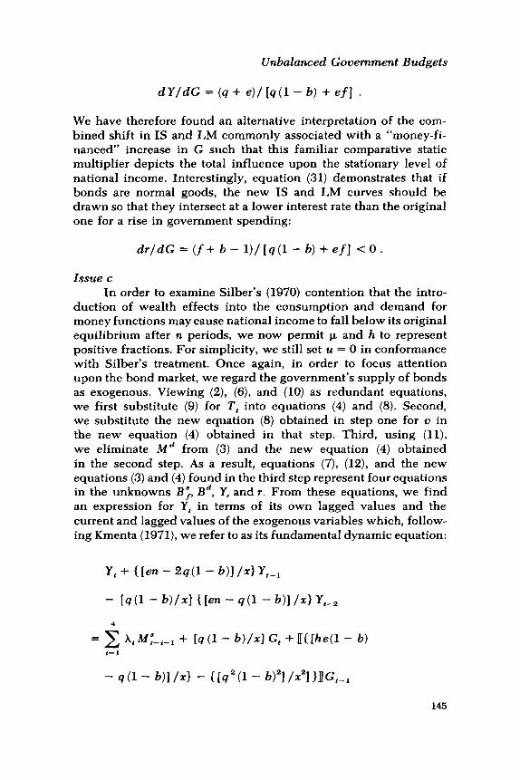
duction of wealth effects into the consumption and demand for money functions may cause national income to fall below its original equilibrium after n periods, we now permit p and h to represent positive fractions. For simplicity, we still set u = 0 in conformance with Silber’s treatment. Once again, in order to focus attention upon the bond market, we regard the government’s supply of bonds as exogenous. Viewing (2), (6), and (10) as redundant equations, we first substitute (9) for T, into equations (4) and (8). Second, we substitute the new equation (8) obtained in step one for u in the new equation (4) obtained in that step. Third, using (ll), we eliminate Md from (3) and the new equation (4) obtained in the second step. As a result, equations (7), (12), and the new equations (3) and (4) found in the third step represent four equations in the unknowns B;, Bd, Y, and r. From these equations, we find an expression for Y, in terms of its own lagged values and the current and lagged values of the exogenous variables which, following Kmenta (1971), we refer to as its fundamental dynamic equation:

Y, + {[en - 29U - b)l /xl Y,-,

- 190 - b)lxl {Ien - 90 - b)l lx) Y,-, 4 = c A, Mu+, + [9 (1 - b)/xl G, + !I{ Pet1 - b) ‘=I

- 90 - b)l lx> - {[9’(1 - @‘I lx”1 IllG,-,

145


+ [9(1 - bj2(9 - eh)/2’1 G,-, + (9blx)(B”,t - Bit-,)

- U{[9(b - 1.4 + Wl - b)l /xl

+ { [g2b(l - b)l l~=lll (B:,-, - q-J

+ [9U - b)lxl{[cl(b - 14 + he(l - b)llx> (B&-z - B&-J

+ constant , (32)

where

n = h(1 - b) -f(l - t.L) )

x= 9(1 -b)+ef,

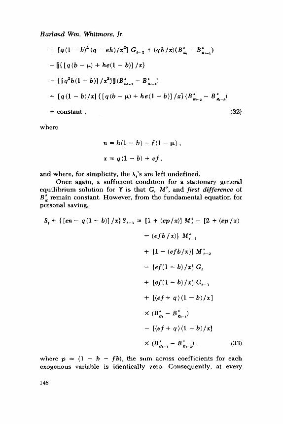
and where, for simplicity, the h,‘s are left undefined. Once again, a sufficient condition for a stationary general

equilibrium solution for Y is that G, M”, and first difference of B: remain constant. However, from the fundamental equation for personal saving,

S, + {[en - ~(1 - b)l /d St-, = 11 + (w/41 MT - P + @p/x)

- (efbl41 Mr-,

+ [1 - (efblx)l MS-*

- [ef (1 - b) lx1 G,

+ [ef(l - b)lrl G,-,

+ tbf + 9)U - b)lxl

x (Bit - B9g,J - [(ef + 9)O - b)lrl

x K,-, - q-J ’ (33)

where p = (1 - b - fb), the sum across coefficients for each exogenous variable is identically zero. Consequently, at every

146


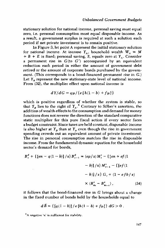
stationary solution for national income, personal saving must equal zero, i.e. personal consumption must equal disposable income. As a result, a government surplus is required at such a solution each period if net private investment is to remain positive.

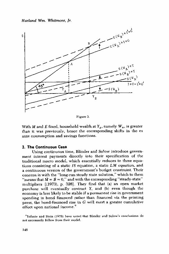
In Figure 3, let point A represent the initial stationary solution for national income. At income Y,, household wealth W, = M + B + E is fixed; personal saving, S, equals zero at Y,. Consider a permanent rise in G (to G ‘) accompanied by an equivalent reduction each period in either the amount of government debt retired or the amount of corporate bonds purchased by the government. (This corresponds to a bond-financed permanent rise in G.) Let Y, represent the new stationary-state level of national income. From (32), the multiplier effect upon national income is

dY/dG = qp/{e [h(l - b) +f~])

which is positive regardless of whether the system is stable, so that Y, lies to the right of Y,.” Contrary to Silber’s assertion, the addition of wealth effects to the consumption and demand for money functions does not reverse the direction of the standard comparative static multiplier for this pure fiscal action if every sector faces a budget constraint. Since taxes are held constant, disposable income is also higher at Y, than at Y, even though the rise in government spending crowds out an equivalent amount of private investment. The rise in personal consumption matches the rise in disposable income. From the fundamental dynamic equation for the household sector’s demand for bonds,

Bf + ([en - o(1 - b)] /xl Bf-‘_, = (ep/r) MT - {[en + ef(1

- WI lx> MI-, - {[ef(l

- b)l /x> G, + (I- efblr)

x (Bit - Bit-,) 7 (34)

it follows that the bond-financed rise in G brings about a change in the fixed number of bonds held by the households equal to

dB = { [q(l - b)] /e [h(l - b) + fp.]} dG > 0 .

“A negative ‘n* is sufficient for stability.

147


Figure 3.

With M and E fixed, household wealth at Y,, namely W,, is greater than it was previously, hence the corresponding shifts in the ex ante consumption and savings functions.

3. The Continuous Case Using continuous time, Blinder and Solow introduce govern-

ment interest payments directly into their specification of the traditional macro model, which essentially reduces to three equations consisting of a static IS equation, a static LM equation, and a continuous version of the government’s budget constraint. Their concern is with the “long-run steady state solution,” which to them “means that ti = & = 0,” and with the corresponding “steady-state” multipliers [(1973), p. 3261. They find that (a) an open market purchase will eventually contract Y, and (b) even though the economy is less likely to be stable if a permanent rise in government spending is bond financed rather than financed via the printing press, the bond-financed rise in G will exert a greater cumulative effect upon national income.’

‘Infante and Stein (1976) have noted that Blinder and Solow’s conclusions do not necessarily follow from their model.

148


The purpose of this section is to examine Blinder and Solow’s (1973) conclusions within the framework presented in Section 2, which we modify to explicitly incorporate government interest payments. Just as in the discrete case, we find that a stationary solution for income and the interest rate is possible without a balanced government budget. Part of the reason is that our continuous model preserves the ex ante relation between the decision to save on the one hand and the decision to accumulate specific assets and/or to retire specific liabilities on the other not only for the government sector but also for the household and business sectors.

According to May (1970), Turnovsky (1977b), and Burmeister and Turnovsky (1977), as the length of the unit time interval approaches zero, the household and business sectors’ (c.f., difference equations (1) and (5), respectively, in Section 2) budget constraints -but not the government sector’s constraint-undergo a peculiar metamorphosis. What previously served as constraints linking ex ante net saving on the income account to planned net purchases of specific assets and to planned net retirements of specific liabilities on the capital account reduce to wealth constraints. In the limit, they argue, the link is broken between asset market decisions and the decision to save.

However, contrary to statements by these authors, the “limit as the length of the unit time interval approaches zero” does not refer to a length of time equal to zero, as a discussion of limits in a standard calculus textbook will attest. Because the continuous analogy of the first difference is the derivative [Goldberg (1958)], the continuous analogy of the budget constraint expressed as a difference equation is the budget constraint expressed as a differential equation-it is not the wealth constraint.”

Using Turnovsky’s notation, let C(T, t) represent the planned consumption rate for time 7, chosen at time t, with y (T, t) and t’(T, t) defined analogously for national income and net taxes. Then the planned amount of consumption, C, over a given time interval, At, is defined as

t+At

C= c (T, t) d7 t

“As mentioned earlier, the budget constraints employed in Section 2 abstract from current portfolio imbalance.

149


and analagously for Y and T. Therefore, equation (1) becomes t+At t+At [y(~, t) - t*(T, t)] d7 = c(T,t)dT + Mf,,, - M:’

* t

+ B:‘,,, - B:‘. (35)

Dividing both sides by At and taking limits as At approaches zero yields

t+At t+At

lim (l/At) [y(T,t) - t”(T,t)] d7 =Al!~O (l/At) c(T, t)dT At-0 t t

+ lim (M:‘,,, - Mf)/At At+0

+ lim (I?:+,,- B,d)/At. At-0

It is true as Turnovsky states [(1977a), p. 531 that lim C At-0

= 0 which does not imply that lim (C/At) = 0. According to At-0

1’Hopital’s rule, this limit is c(t).” Consequently, the continuous version of equation (1) may be written as

y-t*=c++d+I;d, (36)

where y, t*, and c are the instantaneous rates of national income, net taxes, and personal consumption, respectively, while tid and 6” represent the derivatives with respect to time of the household sector’s demands for money~and bonds. Taking government interest payments into account, this constraint becomes

y + rb; - t* z c + ritd + 2;” ) (37)

where r is the rate of interest and bi the supply of government bonds at time t. Unlike a wealth constraint, equation (37) preserves the link between ex ante personal saving (y + rbi - t * - c) and

“Turnovsky makes this point himself in reference to personal saving (1977a, p. 53). Parenthetically, his (and May’s) flow constraint merely defines personal saving.

150


planned accumulations of money, tid, and bonds, 2;“. Assuming ex ante personal consumption depends upon dis-

posable income whereas the demand for money depends upon personal income, equations (2) and (3), respectively, become

c=a+b(y+rb”, - t”) + p(md + bd) ; (38)

7ild =hbd+(h-l)md+f(y+rbi)-qr, (39)

where (39) is obtained by subtracting the demand for money lagged one period from both sides of (3) dividing all terms by At, and taking limits as At + 0.12 Equations (37) through (39) imply the following continuous version of the household sector’s demand for bonds:

6” = -a + (1 - b - f)( y + rb:) + (b - 1) t’

+ 9r + (1 - h - rJ.)m” - (h + p,)bd. (40)

The remainder of the structural equations in the continuous version [corresponding to equations (5) through (12)], respectively, are/given by equations 41 through 48:

i s &; ;

i=d-er;

(41)

(42)

.S b = d - er ; (43)

it* = g + rb: - 6; - ti” ; (44)

t* =u+u(y+rbi); (45)

Y =c+i+g; (46)

md = ms ; (47)

bd=b;+ b;. (48)

“Of course, some of the coefficients in (38) and (39) represent different dimensional constants than they did in equations (2) and (3).

151


Before proceeding further, it is important to point out that because the simple IS-LM model of aggregate demand ignores the impact of public services upon the well-being of the private sector, government expenditures, g, and government interest payments, rbz, merely represent alternative means of providing income to the households.13 Within the confines of the simple macro model, the private sector does not care whether it receives an additional dollar of income in the form of government interest or as the result of government spending on goods and services. The only difference that may arise is that one may choose to count one, but not the other, as earned income. Under these circumstances, a dollar increase in one area accompanied by a dollar reduction in the other will affect national income but leave personal income unchanged.

Letting y ’ = y + rbi denote personal income (less transfers) and treating the money supply and the government’s supply of bonds as exogenous, equations (37) through (48) reduce to the following set of four equations in four unknowns: y *, 7, bd, and b;:

hS=fyQ- qr + hbd + (h - 1)m” ; (49)

6” = [(l - b)(l - u)-f] y’+qr+(l-h-k)m”

- (k + h)bd + (b - 1)~ - a ; (50)

z;” = z;; + 6: ; (51)

&;=d-eer. (52)

From these equations, we obtain differential equation (53) for bd expressed in terms of the exogenous variables:

hd + [e@/A] bd = [(A - ef)lAl(d + 6:) - tef(l - W/Al 0

- [e+ /A]ti” - {e [O + 4~ - fl /A> ms , (53)

where A = q(l - b)(l - u) + ef; 8 = fp + h(1 - b)(l - u); and+=f-(l- b)(l - u). Since (e@/A) > 0, the solution for bd is stable.

l3In a recent paper, Baltensperger (1977) incorporates government expenditures directly into the household sector’s utility function.

152


Substituting (49) into (50) yields an expression for y* in terms of bd and the exogenous variables:

Y * = [l/(1 - b)(l - u)] [6” + riz”

+k(m”+bd)+(l-b)v+a]. (54)

It is clear from (53) and (54) that constant levels of u, v, m”, and 6: are sufficient to achieve stationary levels of both b” and y*; once again, a balanced budget is not required to achieve a stationary-state equilibrium for (personal) income. The real supply of government bonds may change. Also, since the solution for bd is stable, the solution for y* is stable.

Substitution of (54) into the government’s budget constraint yields expression (55) for government expenditures:

+ [l/(1 - u)] v + [ua/(l - b)(l - u)]

+ {[l - b(1 - u)] / [(l - b)(l - u)]}r;l”

+ [u~J(l - b)(l - u)] ms . (55)

With u, v, m* and 6: fixed, g changes in the opposite direction dollar for dollar with a change in government interest payments.

Since at a stationary solution a government surplus is necessary for positive net investment to take place, at such a solution, government interest payments will be falling over time as the government continues to retire its outstanding debt. Consequently g will rise over time. Depending upon whether we choose to include government interest payments as part of earned income, national income may be viewed as steadily rising at a stationary solution for personal income.

If the government holds corporate bonds, national income will tend to exceed personal income by the amount of corporate interest received by the government. If the government applies its fixed surplus to acquiring new corporate bonds, its interest income from corporate bonds will continue to grow over time. In order to maintain the constant surplus, government expenditures must grow dollar for dollar with this interest income. Once again, although national income continues to grow with the increase in

153


government spending, a stationary level of personal income is maintained.

Let m” = 0 (i.e., mS = rii) and let &“, = - k, where fi and k are positive constants. If the government permanently raises the au- tonomous component of government spending [which we define as the sum of the last five terms on the right-hand side of (55)] by reducing the rate k at which it either retires its own outstanding debt or purchases corporate bonds, it will, according to (53) and (54) respectively, affect the stationary-state levels of bd and y” as follows:

dgd/ddi = [q(l - b) (1 - u)]/ [efk + eh(1 - b) (1 - u)] > 0 ;

d$’ /d&z = ~9/ [efp, + eh(1 - b) (1 - u)] > 0. (56)

Consequently, a permanent reduction in government surplus financed by a curtailed rate of debt retirement expands personal (and national) income, just as Blinder and Solow maintain.14 However, contrary to their results, an open-market purchase of bonds, dfi > 0 (which leaves A” = 0 and 6: = - k), also expands personal (and national) income. In particular we see that

dii”ldfi = {P/ [(l - b) (1 - u)]) [(dbd/dCi) + l] ,

=P/[fp+h(l-b)(l-u)] >O. (57)

Furthermore, a permanent reduction in the government surplus financed initially by an increase in m but always thereafter by reduced government lending produces the following multiplier effect upon the stationary level of personal income (dh”, = dill > 0) :

dij”/dhz = [p.(9+ e)]/{e[fk++(l - b) (1 - u]} > 0. (58)

A partly money-financed increase in government spending is more expansionary than the pure fiscal result displayed in (56).15 This is entirely consistent with the relative magnitudes of the comparative

14This appears to contradict Christ’s [(1978), p. 661 result presented in row 4 column 3 of his Table 2.

“Of course, a rise in g financed exclusively by additional money will not yield a new stationary solution. Therefore, the multiplier attached to this policy will not even be defined.

154


static multipliers attached to a shift to the right in IS alone, and to a combined shift to the right in IS and LM in the simple-static framework for a bond-financed and a (partly) money-financed rise in government spending, respectively.

4. Conclusion In summary, when each sector in the simple IS-LM framework

is viewed as subject to a budget constraint, as Turnovsky and others suggest, then recent statements to the contrary notwithstanding, the standard comparative static multipliers do indeed incorporate not only the government’s budget constraint but also changes in private asset holdings. Interestingly, a stationary solution for national income under the dynamic specification of this model permits the real supply of government bonds to change at a constant rate. A given static intersection of IS and LM can represent stationary levels of income and the rate of interest over time even though commodity prices are fixed and the government’s budget is unbalanced. The budget constraint approach also permits an interpretation of a combined once-for-all shift in IS and LM (commonly associated with a “money-financed” rise in government spending) such that the corresponding familiar comparative static multiplier represents a change in national income between stationary states.

Introducing wealth effects into the consumption and demand for money functions to correspond to Silber’s specification of the traditional macro model, we find that with budget constraints facing every sector, an entirely bond-financed permanent increase in government spending definitely expands the stationary-state level of national income. Parenthetically, the positive influence of this policy action upon national income holds no matter whether the system is stable or not.

Proceeding to a continuous version of the traditional model which also takes government interest payments explicitly into account, we find that the budget constraints facing the household and business sectors do not-contrary to the result of Turnovsky, May, and others-reduce to wealth constraints as the length of the planning interval approaches zero. Also, contrary to Blinder and Solow’s findings, an open market purchase continues to be expansionary. A rise in government spending accompanied by a reduction in the rate of government debt retirement or (corporate debt absorption) also expands the stationary level of personal income just as Blinder and Solow suggest. However, a finite increase in

155


the money supply to pay for the initial rise in government spending is, contrary to their results, even more expansionary.

In short, we find the simple comparative static multipliers can be viewed as containing more effects than previously have been attributed to them, and that neither the signs nor the relative magnitudes of the standard monetary and fiscal policy multipliers are affected by the addition of wealth effects in the consumption and demand for money functions, the explicit introduction of government interest payments, or the choice of a continuous or discrete time setting for the dynamic versions of this model,

Received: January, 1979 Revised version received: June, 1979

References Allen, R.G.D. Macroeconomic Theory. New York, St. Martin’s Press,

Inc., 1967. Baltensperger, E. “Government Expenditure Policies in Equilibri-

um and Disequilibrium.” Kyklos 30 (3/ 1977): 421-42. Blinder, A.S. and R.M. Solow. “Does Fiscal Policy Matter?” Journal

of Public Economics 2 (November 1973): 319-37. -. and -. “Does Fiscal Policy Matter? A Correction.”

Journal of Public Economics 5 (February 1976a): 183-84. -. and -. “Does Fiscal Policy Still Matter? A Reply.”

Journal of Monetary Economics 2 (November 1976b): 501-10. Christ, C. “A Simple Macroeconomic Model with a Government

Budget Restraint.” Journal of Political Economy 76 (January- February 1968): 53-67.

-. “Some Dynamic Theory of Macroeconomic Policy Effects on Income and Prices under the Government Budget Restraint.” ]ournal of Monetary Economics 4 (January 1978): 45-70.

Foley, D.K. “On Two Specifications of Asset Equilibrium in Macroeconomic Models.” Journal of Political Economy 83 (April 1975): 303-24.

Goldberg, S. Introduction to Difference Equations. New York: John Wiley & Sons, Inc., 1958.

Hansen, B. A Survey of General Equilibrium Systems. New York: McGraw-Hill Book Co., 1970.

Infante, E.F. and J.L. Stein. “Does Fiscal Policy Matter?” Journal of Monetary Economics 2 (November 1976): 473-500.

Kmenta, J. Elements of Econometrics. New York: The Macmillan co., 1971.

156


May, J. “Period Analysis and Continuous Analysis in Patinkin’s Macroeconomic Model.” Iournal of Economic Theory 2 (March 1970): l-9.

Metzler, L. “Wealth, Saving, and the Rate of Interest.” JournaZ of Political Economy 59 (April 1951): 93-116.

Meyer, L.H. “The Balance Sheet Identity, the Government Financ- ing Constraint, and the Crowding-Out Effect.” Journal of Mone- tary Economics 1 (January 1975): 65-78.

Ott, D.J. and A. Ott. “Budget Balance and Equilibrium Income.” Journal of Finance 20 (March 1965): 71-77.

Patinkin, D. Money, Interest and Prices. Evanston, Illinois: Row, Peterson & Co., 1956.

Pesek, B. and T.R. Saving. The Foundations of Money and Banking. New York: The Macmillan Co., 1968.

Ritter, L.S. “Some Monetary Aspects of Multiplier Theory and Fiscal Policy.” Review of Economic Studies 23 (2/1956): 126-31.

Silber, W.L. “Fiscal Policy in IS-LM Analysis: A Correction.” Journal of Money, Credit, and Banking 2 (November 1970): 461-72.

Tobin, J. “A General Equilibrium Approach to Monetary Theory.” Journal of Money, Credit, and Banking 1 (February 1969): 15-29.

Turnovsky, S. J. “Monetary Policy, Fiscal Policy and the Government Budget Constraint.” Australian Economic Papers 14 (December 1975): 197-215.

-. “On the Formulation of Continuous Time Macroeconomic Models with Asset Accumulation.” Znternational Economic Re- view 18 (February 1977a): 1-28.

-. Macroeconomic Analysis and Stabilization Policy. New York: Cambridge University Press, 1977b.

-. and E. Burmeister. “Perfect Foresight, Expectational Con- sistency and Macroeconomic Equilibrium.” Journal of Political Economy 85 (April 1977): 379-93.

157

unbalanced government budgets, private asset holdings, and the traditional comparative static...

Documents