(un-)predictability in bond returns
TRANSCRIPT

COPENHAGEN BUSINESS SCHOOL
MASTER’S THESIS
(Un-)Predictability in Bond Returns
Benchmarking deep learning architectures out of sample
Abstract
We conduct an out of sample study of predictors of excess returns on US Treasuries. We add tothe group of considered predictors by including Artificial Neural Networks (ANN). We find that the bestpredictor of excess returns is the historical mean and thus fail to reject the Expectations Hypothesis out ofsample. ANNs converge on the same signal recovered by a linear combination of forward rates, and non-linear combinations of yields do not have predictive power in excess of this linear combination. Laggedforward rates and real time macroeconomic data do not either, and so we do not find a hidden factor inthe yield curve.
MSC IN ADVANCED ECONOMICS AND FINANCEMads Bibow Busborg Nielsen, Kai Rovenich
supervised by
Paul WHELAN
Characters: 243.647 (107.1 normal pages)
15.05.2017

Contents
1 Introduction 1
2 Terminology 4
3 Literature Review 53.1 Literary Overview . . . . . . . . . . . . . . . . . . . . . . . . . . . . . . . . . . . . . . . . 5
3.2 Theoretical Bond Pricing Literature . . . . . . . . . . . . . . . . . . . . . . . . . . . . . . 8
3.2.1 Expectation Hypothesis . . . . . . . . . . . . . . . . . . . . . . . . . . . . . . . . 8
3.2.2 Affine term structure models . . . . . . . . . . . . . . . . . . . . . . . . . . . . . . 10
3.2.3 Market price of risk . . . . . . . . . . . . . . . . . . . . . . . . . . . . . . . . . . . 11
3.2.4 Specifications of the market price of risk process . . . . . . . . . . . . . . . . . . . 17
3.2.5 Affine models with a hidden factor . . . . . . . . . . . . . . . . . . . . . . . . . . . 20
3.3 Empirical bond pricing literature . . . . . . . . . . . . . . . . . . . . . . . . . . . . . . . . 23
3.3.1 Explicit test of time varying risk premia . . . . . . . . . . . . . . . . . . . . . . . . 25
3.3.2 Decomposing the yield curve . . . . . . . . . . . . . . . . . . . . . . . . . . . . . . 26
3.3.3 Predictors outside the yield curve . . . . . . . . . . . . . . . . . . . . . . . . . . . 27
4 Analytical Tools and Concepts 294.1 Artificial Neural Networks (ANN) . . . . . . . . . . . . . . . . . . . . . . . . . . . . . . . 29
4.1.1 Training vs. Validation vs. Testing . . . . . . . . . . . . . . . . . . . . . . . . . . . 30
4.1.2 Architecture . . . . . . . . . . . . . . . . . . . . . . . . . . . . . . . . . . . . . . . 30
4.1.3 Forward propagation . . . . . . . . . . . . . . . . . . . . . . . . . . . . . . . . . . 31
4.1.4 Gradient Descent . . . . . . . . . . . . . . . . . . . . . . . . . . . . . . . . . . . . 32
4.1.5 Backpropagation . . . . . . . . . . . . . . . . . . . . . . . . . . . . . . . . . . . . 33
4.1.6 Learning . . . . . . . . . . . . . . . . . . . . . . . . . . . . . . . . . . . . . . . . 35
4.1.7 Ensembles of ANNs . . . . . . . . . . . . . . . . . . . . . . . . . . . . . . . . . . 38
4.2 Principal Component analysis . . . . . . . . . . . . . . . . . . . . . . . . . . . . . . . . . 39
4.3 Finite differences method: basis and extension for ANNs . . . . . . . . . . . . . . . . . . . 40
4.3.1 Forward, backward, and central differences . . . . . . . . . . . . . . . . . . . . . . 40
4.3.2 Extension: The non-linearity score RMSDL . . . . . . . . . . . . . . . . . . . . . . 42
4.4 Generalized degrees of freedom (GDF) . . . . . . . . . . . . . . . . . . . . . . . . . . . . 44
4.5 Generalized method of moments (GMM) for regression . . . . . . . . . . . . . . . . . . . . 45
5 Data Description and Reproduction of Established Results 485.1 Descriptive statistics . . . . . . . . . . . . . . . . . . . . . . . . . . . . . . . . . . . . . . 48
5.2 Reproduction of Cochrane Piazzesi in sample results and combination with macroeconomic
data . . . . . . . . . . . . . . . . . . . . . . . . . . . . . . . . . . . . . . . . . . . . . . . 51
i

6 Methodology 536.1 Statistical measures to rate out of sample performance . . . . . . . . . . . . . . . . . . . . . 54
6.2 Economic measures to rate out of sample performance . . . . . . . . . . . . . . . . . . . . 55
6.3 Description of forecasting approaches . . . . . . . . . . . . . . . . . . . . . . . . . . . . . 56
6.3.1 Unconditional expectation . . . . . . . . . . . . . . . . . . . . . . . . . . . . . . . 56
6.3.2 Cochrane-Piazzesi approach . . . . . . . . . . . . . . . . . . . . . . . . . . . . . . 56
6.3.3 Cochrane-Piazzesi approach using real time macroeconomic data . . . . . . . . . . 57
6.3.4 ANN architectures . . . . . . . . . . . . . . . . . . . . . . . . . . . . . . . . . . . 58
6.3.5 Sample periods and training time . . . . . . . . . . . . . . . . . . . . . . . . . . . 62
7 Analysis and Discussion of results 627.1 Results of statistical tests . . . . . . . . . . . . . . . . . . . . . . . . . . . . . . . . . . . . 62
7.1.1 Benchmark performance . . . . . . . . . . . . . . . . . . . . . . . . . . . . . . . . 62
7.1.2 ANN prediction results . . . . . . . . . . . . . . . . . . . . . . . . . . . . . . . . . 65
7.2 Absolute performance . . . . . . . . . . . . . . . . . . . . . . . . . . . . . . . . . . . . . . 68
7.3 Performance over time . . . . . . . . . . . . . . . . . . . . . . . . . . . . . . . . . . . . . 73
7.4 Results of economic tests . . . . . . . . . . . . . . . . . . . . . . . . . . . . . . . . . . . . 75
7.4.1 Benchmark performance . . . . . . . . . . . . . . . . . . . . . . . . . . . . . . . . 75
7.4.2 ANN predictions . . . . . . . . . . . . . . . . . . . . . . . . . . . . . . . . . . . . 77
7.4.3 Performance over time . . . . . . . . . . . . . . . . . . . . . . . . . . . . . . . . . 79
7.5 (Generalized) degrees of freedom . . . . . . . . . . . . . . . . . . . . . . . . . . . . . . . 82
7.6 Deep dive into model predictions . . . . . . . . . . . . . . . . . . . . . . . . . . . . . . . . 84
7.7 ANN Decomposition . . . . . . . . . . . . . . . . . . . . . . . . . . . . . . . . . . . . . . 91
8 Conclusion 95
A APPENDIX RMDSL example 98
B APPENDIX macro dataset 99
C APPENDIX ANN decomposition 101
D APPENDIX Technical details 103
References 104
ii

1 Introduction
In this paper, we explore the predictability of excess returns of longer maturity US government bonds.
According to the Expectations Hypothesis (EH), the return of holding a longer maturity bond while borrow-
ing at the one year yield should be constant over time. Fama and Bliss (1987), Campbell and Shiller (1991)
and Cochrane and Piazzesi (2005) show convincing evidence against this. Furthermore, they show that
rather than predicting short rates, forward rates predict excess returns. While the cross-section of yields is
summarized well by a three factor decomposition (Litterman and Scheinkman (1991)), Cochrane and Pi-
azzesi (2005) show that factors beyond these three matter for the in sample predictability of excess returns.
Ludvigson and Ng (2009) show that outside factors, not summarized in the cross-section of yields, improve
predictability over a linear combination of forward rates used in Cochrane and Piazzesi (2005) - also in sam-
ple. This is a puzzling result since information available at one point in time should be reflected in prices
at that same time. Duffee (2011) suggests a hidden factor model in which one or more factors might not be
reflected in yields today and should still be able to forecast excess returns in the future. Besides macroeco-
nomic data and lagged forward rates, which are candidates for this hidden factor found in earlier research
(Cochrane and Piazzesi (2005), Ludvigson and Ng (2009)), we investigate whether non-linear combinations
of yields could play a role.
There have been significant advances in data analysis and -science in recent years. The availability of pow-
erful computers, coupled with larger amounts of data, have brought forward a class of models that are much
more powerful, and much less restricted than traditional models. The area of deep learning relies on many
data points and sufficient computing power and requires the researcher to make very little assumptions about
the underlying model beforehand. These models are able to fit any underlying function, given enough time
and degrees of freedom (Winkler and Le (2017)), including non-linear relationships.
We investigate out of sample predictability of bond returns using aforementioned models. Our approach
is the following: We first confirm or reject earlier in sample results in an out of sample set-up, similar to
the analysis Campbell and Thompson (2008) conducted for established predictive relationships in the stock
market. We then compare the performance of predictors using linear combinations of forward rates to the
performance of models using non-linear combinations. If we can beat the performance of the linear com-
bination out of sample, we can conclude that non-linear relationships in the data have predictive power in
excess of the linear combination. If we can beat the performance of a model including macroeconomic data
(in the spirit of Ludvigson and Ng (2009)) or lags of forward rates, we can hypothesize that non-linear com-
binations of forward rates reflect what has been suspected to be a ”hidden” factor in the yield curve. That is
the data-analysis part of the thesis.
Because of their complex structure, deep neural networks are considered a black box when it comes to
interpretability. We incorporate that objective into our approach from the outset. Before fitting our models
1

we choose a number of base architectures that we impose different restrictions on. After fitting we combine
classical statistical analysis of our models as predictors with the application, and in one case extension of,
numerical methods. We use these tools in a sensitivity analysis to decompose and better understand our
results. We also use our predictions in a trading strategy in order to test our results economically.
We find that the unconditional mean, on average, is the best predictor regardless of maturity of bond in
question, the sample period and training window. The unconditional mean does, however, not capture the
dynamics of excess returns, and even after a correction for out of sample noise the mean is not significantly
correlated with excess returns. In contrast, predictions based on the regression of excess returns on five
forwards as proposed by Cochrane and Piazzesi (2005) are. We conjecture that the five forward rates find a
more meaningful relation than the mean, but noise obscures the signal to a degree where it is not helpful out
of sample. The results of our economic test, the trading strategy, corroborates this idea: returns to trading on
the prediction of the mean beat the returns to predictions conditioning on the forward rates. We observe that
long term average realized excess returns are negatively correlated with long term trends in yields. Further-
more, any other predictor than the rolling unconditional mean exhibits long term average positive correlation
with yields, leading to the former loosing out to the latter in root mean squared error (RMSE) terms. In
consistently failing to get the level right out of sample, we do not find significant predictability in excess
returns conditioning on forward rates. As such we cannot reject the Expectation Hypothesis.
For the relative performance of the group of predictors that excludes the mean, we find remarkably simi-
lar performance out of sample. For previously described predictors conditioning on information in excess of
current yields we find improvement of in sample results. This is in accordance with earlier studies. However,
the improvements either do not materialize out of sample, or have directly detrimental effects. Based on these
results we pick the the Cochrane and Piazzesi (2005) regression predictions as the benchmark for a more in
depth analysis of the performance of the Artificial Neural Networks (ANNs) which are our contribution to
the group of predictors. A minor finding is that the ANNs can achieve on par in sample performance as the
models including information outside the yield curve, without sacrificing out of sample performance. This
finding, however, relates to the broader field of more flexible predictors. We see this as an indication that
these in sample gains may be driven by model flexibility as opposed to conditioning on a fuller (relevant)
information set. The outcome is over-fitting: in an application of the method of generalized degrees of free-
dom we find support for this line of thinking in the correspondence between the ranking of the estimated
degrees of freedom for our ANNs and their in sample performance; the picture out of sample is less clear,
but the tendency to trade off more freedom for worse performance is more pronounced.
Our takeaway from both the temporal and cross-sectional analysis is that the ANNs seem to recover the
same signal as the benchmark. For the training periods that we base predictions on, we consider two rolling
windows of respectively 10 and 20 years. Both statistical and economic indicators points to the latter being
more meaningful than the former, with all models achieving lower RMSE, higher correlation with realized
2

returns, and positive cumulative returns. While the relative results of our generalized degrees of freedom
estimation show a clear pattern, the estimated degrees of freedoms for the ANNs are in absolute terms only
about 30% higher than the ones for the Cochrane and Piazzesi (2005) regression model. We find this effect
due to the early stopping we apply in the training of the ANNs to avoid over-fitting. We find a stronger trade-
off between freedom and out of sample performance for the ANNs than for the linear models. To explain
it, we explicitly investigate the effect of the non-linear features of the ANNs on the predictions. We find
that our measure of non-linearity, root mean squared distance to linear (RMSDL) in regressions controlling
for the squared errors made by the Cochrane and Piazzesi (2005) predictor is significant in predicting the
squared error made by our architectures1 .
We first define some of the vocabulary used throughout the thesis. Next, we give a brief general overview
of the literature related to our study. After the general overview, we dig deeper into theoretical material
providing our analysis with context, before moving on to an overview of empirical results that have been
produced in the area so far. After setting the scene, we go through the main analytical tools used in the study.
The largest section is on Artificial Neural Networks, reflecting the relative novelty of this methodology in
the area of asset pricing. We then describe the data and reproduce established results, before describing the
specific methodological set up for analysis. We finish the thesis with an analysis and discussion of our results
and a brief conclusion on our findings.
1All regressions has coefficients on RMSDL that are significant at the 5% level, except for one with a p-value of 11%. Standarderrors are corrected for serial correlation and heteroskedasticity; we find coefficients to be significant both in a statistical sense andin terms of the impact of a one standard deviation change in RMDSL.
3

2 Terminology
In this section, we introduce some general terminology about bonds, the subject of our study. When we talk
about bonds, we are referring to U.S. Treasury bonds. These bonds are claims to a certain future cash flow
that are subject to a very small (and therefore negligible) default risk. Bonds usually have coupons, i.e. cash
flows that are paid semi-annually every year until the maturity of the bond. These coupon-bearing bonds can
be decomposed into series of zero coupon bonds, which have only two cash flows: One in the beginning,
when the buyer pays for the bond, and one in the end when they are paid the nominal amount. For simplicity
we limit our discussion to zero-coupon bonds.
We distinguish between discrete and continuous time with slightly different notation. Overall, we consider
discrete time; the use of continuous time is limited to the section on theoretical literature. Below, we define
the main variables of interest in discrete time and where relevant we include the continuous time equivalent
in square brackets [].
We denote the price of a zero-coupon bond with a maturity n at time t as P (n)t in the discrete case and
as P (t, T ) where T is the time of maturity in the continuous. The nominal amount is normalized to one:
P(0)t = 1 [P (T, T ) = 1]
Lower case letters indicates logs for prices, yields, and returns:
p(n)t = log(P
(n)t ) [p(t, T ) = log(P (t, T ))]
We define the yield to maturity (YTM) of a bond as the annualized return the bond pays during its maturity.
The log-YTM can simply be written as:
y(n)t = − 1
np
(n)t
[y
(T−t)t = − 1
T − tp
(T−t)t
]The yields for zero-coupon bonds that can be observed today contain information about the price of borrow-
ing without default risk not only from today to different points in the future, but also about the price at which
transferring funds between different points in the future can be locked in today. We call the price of such a
transaction (e.g., lending money at time t + 3 and getting it back at time t + 4) today a forward rate ft(4)
and calculate it as:
ft(n) = p(n−1)t − p(n)
t
This calculation reflects that the forward rate is the price that has to be paid today for a portfolio that has a
positive cash flow of one at time t + n and a negative cash flow at time t + n − 1. In practice, we would
buy one zero coupon bond of maturity n and short exactly as many maturity n− 1 bonds as it takes to make
4

the cash flow 0 at time t. We furthermore define holding period returns as the return of holding a bond of
maturity n for y years:
hpr(n)t+y = p
(n−y)t+y − p(n)
t
Since we are interested in risk compensation and expected changes in interest rates, we also need a measure
for the difference between longer term and shorter term interest rates. We define holding period excess
returns as follows:
hprx(n)t+y = hpr
(n)t+y − y
(1)t
Finally, we adopt the use of the terms P and Q measure that are widely spread in the financial literature to
describe respectively real world physical processes, and risk-neutral equivalents. Where it is relevant we
expand on the meaning of this relationship, but the general coverage is rather a subject for a good textbook;
our reference is Bjork (2009).
3 Literature Review
In this section, we motivate our study by giving an overview of past and recent problems that have been
considered in the area of bond predictability. We first provide a high-level overview of relevant papers
and thereafter cover the implications of a number of central papers more in depth. This in-depth coverage
introduce both the theoretical background and the established empirical context for our thesis and is split
into two parts accordingly.
3.1 Literary Overview
The Expectations Hypothesis of the term structure (EH), which roughly speaking considers long rates to be
expectations of short rates, has been around for a long time in a verbal rather than mathematical form (Sangv-
inatsos (2010)). The general idea that expectations of short rates influences long rates even pre-dates the first
theoretical work (Cox, Ingersoll, and Ross (1981)), to which early attributions where made by Lutz (1940),
Hicks (1946), and Macaulay (1938). In the theoretical part below we will give a more in depth coverage
of the later reformulation in continuous time by Cox, Ingersoll, and Ross (1981), in which they consider
different formulations of EH and rule out most of them by requiring consistency with a rational expectations
equilibrium.
One of the great advantages of the EH is its simplicity, which makes it easily testable. Fama and Bliss (1987)
and Campbell and Shiller (1991) both find evidence against the EH. Fama and Bliss (1987) finds that forward
rates predict excess returns on bonds of the same maturity, and not future yields. Campbell and Shiller (1991)
finds that the yield spread between two different maturity bonds predicts the longer maturity bond yield to
decrease over time if the spread is large, which also contradicts the EH. There exist arguments against the
validity of some of the tests due to finite sample properties (e.g. Bekaert and Hodrick (2001)), who test the
5

small sample properties of several vector autoregressive tests of the EH. They find that a Lagrange multiplier
test has good small sample properties and that the evidence against the EH is considerably weakened. Sarno,
Thornton, and Valente (2007) use the same test, while conditioning on macroeconomic information and in-
cluding more yields and get results suggesting a rejection of the EH.
While EH can be considered an early model for explaining the term structure of interest rates, this term
is in modern times associated with a more complex class of models. An early example of such a model was
introduced in Vasicek (1977). The model describes a stochastic process in continuous time, an approach to
modelling in financial economics popularized by Merton in the early 1970s (Fan and Sundaresan (2000)).
The stochastic process in Vasicek (1977) is, as opposed to papers modelling stock-prices (Black and Sc-
holes (1973), Merton (1973)), an OrnsteinUhlenbeck process which has the property of mean-reversion. The
one factor in the model is the short rate. Cox, Ingersoll, and Ross (1985) (CIR) refined this interest rate
model by making volatility depend on the level of the interest rate, which prevents the model from produc-
ing negative interest rates. The models make different assumptions about the market price of risk, which
for certain modelling approaches has implications for option pricing as described in Bollen (1997). The
implications of these assumptions for the investigations of the EH in the context of building models of the
yield-curve will be covered in the theoretical section below. Cox, Ingersoll, and Ross (1985) include an ex-
tension to models with more factors, which may be more reasonable than the one-factor set-up as indicated
by the findings of Litterman and Scheinkman (1991). The authors introduce a principal component analysis
of the yield curve, finding that the cross section of yields is well summarized statistically by three factors.
Nelson and Siegel (1987) introduced a three factor model for the yield curve, depending on level, slope and
curvature of the yield curve. While the model is still relatively simple, it fits the yield curve well and is
widely used in practice. A major difference between this model and the Vasicek or CIR model, is that the
latter defined cross-sectional restrictions to ensure no-arbitrage, whereas the former is a (purely) statistical
model. Vasicek or CIR both belong to the affine class of term structure models, described in the seminal
coverage of a multi-factor set up by Duffie and Kan (1996) as models in which the yield at any time for any
maturity can be expressed as an affine transformation of the factors in the model. Piazzesi (2010) summarize
a large body of work from previous years and includes the condition that the stochastic processes of the
factors are affine under the risk-neutral measure.
The key feature of the term structure for our work is excess return predictability. The early literature on
tests of the EH (Fama and Bliss (1987), Campbell and Shiller (1991)) has led to a new branch of literature
exploring the predictability of excess bond returns. The EH predicts that excess returns should be constant
over time. In a regression of something on these excess returns all predictability should thus be captured in
the intercept. Several studies find extensive evidence for the time-variability of excess returns. Cochrane and
Piazzesi (2005) find large predictability in a tent-shaped linear combination of forward rates with R2 up to
44% in sample. These results apply across markets: The evidence is in fact stable across different countries
(Campbell and Hamao (1992), Ilmanen (1995)) and extends to other asset classes (Campbell (1987)). Relat-
6

ing this result back to term structure models, Cochrane and Piazzesi (2005) point out that factors beyond the
first three matter for predictability, although they do not contribute much in describing the cross section. This
predictability arising from the inclusion of fringe factors is stable over different countries as well (Dahlquist
and Hasseltoft (2013), Hellerstein (2011)). Campbell and Thompson (2008) reproduce predictive relation-
ships in the stock market out of sample and find that ”beating” the historical mean is inherently difficult due
to noise in the data.
The importance of fringe factors for predictability has shown that a three factor model might be a too sim-
plified version of the world. Dai and Singleton (2000) argue that although three-factor affine term structure
models are potentially very rich, many impose strong and potentially over-identifying assumptions on the
term structure and fail to describe important features of interest rates. Duffee (2002) observes that existing
affine term structure models can generate time-varying excess returns, but only with variation in the variance
of risk. Because of the non-negativity of variances the expected excess returns with low means and high
volatilities that are implied by the slope of the yield curve generally observed in data on Treasury bonds re-
quires some underlying factor to be highly skewed; a proposition rejected by the data. He introduces a class
of models that circumvents this problem by allowing risk compensation to vary independently of interest
rate volatility. In a similar set-up Dai and Singleton (2002a) show that a Gaussian three-factor model can
generate time-varying risk-premia that, when used as an adjustment, can establish the relation between yield
spreads and future changes in short rates rejected in raw data by Campbell and Shiller (1991). Cochrane
and Piazzesi (2008) set up an affine term structure model that displays the same predictability they have
found in their 2005 paper by including a fourth forecasting factor. Duffee (2011) points out that affine term
structure models allow for state variables that are orthogonal to (or unspanned by) the yield curve, and as
such ’hidden’ with respect to current yields. He argues that the assumption of invertibility, which is implicit
in much literature on affine models, is not necessary and finds empirical support for his hypothesis of a hid-
den factor: Only half of the variation in bond risk premia can be detected using the cross section of yields.
One suspect for that hidden factor are macroeconomic indicators: Earlier studies (Lo and Mackinlay (1997))
show that macroeconomic data can predict yields. Ang and Piazzesi (2003) are able to predict up to 85% of
the variation in yields using vector autoregression of macroeconomic data. Wu and Zhang (2008) show that
inflation and real output shocks have strong positive effects on treasury yields. Ludvigson and Ng (2009)
explicitly relate predictive power in macroeconomic data to the predictive power in the yield curve, namely
by including the Cochrane and Piazzesi (2005) forecasting factor. They find substantial forecasting power
in excess of the tent-shaped factor. Ghysels, Horan, and Moench (2014) point out flaws in the methodology
used by Ludvigson and Ng (2009), namely the fact that historical macroeconomic data is corrected later in
time and therefore includes future information. When including only real time data, they find the predic-
tive power in the macroeconomic data is drastically reduced. Coroneo, Giannone, and Modugno (2016) find
macroeconomic factors to be the primary source of risk unspanned by the yield curve. Feldhutter, Heyerdahl-
Larsen, and Illeditsch (2013) explore the possibility that yields and market prices of risk could be non-linear
functions of Gaussian factors: These non-linear functions might not have been captured by regression and
7
other studies that focussed on fitting linear relationships in the data.
3.2 Theoretical Bond Pricing Literature
3.2.1 Expectation Hypothesis
As described in the above overview, the Expectations Hypothesis emerged as a number of economic preposi-
tions about the term structure of interest rates formulated in prose rather than mathematical equations. Cox,
Ingersoll, and Ross (1981) formalize these ideas in a continuous time set-up. A red string that runs through
their treatment is a word of warning on developing theory under certainty and adapt to introduce uncertainty.
In an instructive use of Jensen’s inequality they rule out the strongest form of the Expectations Hypothesis:
Expected returns of any series of investments for a given holding period must be equal.
E[P (t1, T1)
P (t0, T1)× P (t2, T2)
P (t1, T2)× · · · × P (tT , TT )
P (tT−1, TT )
]=
1
P (t0, TT )= µ
Focusing on two periods, a one-period bond with a certain pay-off of 1 should have the same return as the
expected one period return on a 2 period bond. Meanwhile the certain return to a two period bond should
equal the expected return of rolling over a shorter bond
1
P (t0, T1)=
E[P (t1, T2)]
P (t0, T2)
1
P (t0, T2)=
1
P (t0, T1)E[
1
P (t1, T2)
]Rearranging both equalities
1
E[P (t1, T2)]=P (t0, T1)
P (t0, T2)=P (t0, T1)
P (t0, T2)= E
[1
P (t1, T2)
]If P (t1, T2) is a random variable Jensen’s inequality implies that
1
E[P (t1, T2)]> E
[1
P (t1, T2)
]which implies that this version of the EH only works under certainty.
Yield to maturity Expectations Hypothesis Cox, Ingersoll, and Ross (1981) discuss other possible for-
mulations of the Expectations Hypothesis of which two are of interest here. The yield to maturity Expecta-
tions Hypothesis, which states that the yield to maturity is the expected short rate over the period.
− ln(P (t, T ))
T − t= y
(T−t)t =
Et[∫ Tt r(u)du]
T − t=
∫ Tt Et[r(u)]du
T − t(1)
Piazzesi (2010) identifies this particular version as simply: the Expectations Hypothesis. Because of the
linearity of the expectations operator and the integral, the expectation of the integral over rates and the
8

integral over expected rates are equal.
Local Expectations Hypothesis For the local Expectations Hypothesis Cox, Ingersoll, Ross and Piazzesi
agrees on the name which is inspired by the fact that the expectation of instantaneous return over a given
infinitesimal period is equal across maturities and that this rate is the instantaneous short rate. In what
Piazzesi (2010) warns is a misuse of notation (but a useful one) this can be expressed as
E[dP (t, T )
P (t, T )
]= r(t)dt
In integral form, the hypothesis has the interpretation that the price of a zero coupon bond is the pay-off of 1
discounted at the (stochastic) instantaneous short rate
P (t, T ) = Et[e−∫ Tt r(u)du] (2)
and Piazzesi (2010) shows that the local Expectations Hypothesis can be formulated as the physical measure
P coinciding with the risk-neutral measure Q. As we will show below this corresponds to the market price
of risk being zero in affine term structure models.
Yields under the local Expectations Hypothesis are given by
y(T−t)t = − ln(P (t, T ))
T − t=− ln
(Et[e−
∫ Tt r(u)du]
)(T − t)
which will differ from (1) by a Jensen’s inequality term that will depend on the distribution of the random
variable∫ Tt r(u)du.
Link to empirical work A discretized version of the yield to maturity Expectations Hypothesis (1) applied
in empirical work (e.g. Campbell and Shiller (1991)) adds a term that varies with time to maturity, but is
constant over time to allow for a constant risk-premium, which maintains the central idea that the dynamics of
the yield curve are driven by expectations about short rates, but accommodates the stylized fact that the yield
curve on average is upward sloping (Piazzesi (2010)). To distinguish between the version with a premium
and one without the latter can be referred to as the pure Expectations Hypothesis (Sangvinatsos (2010)).
y(n)t =
1
T
T−1∑s=t
(E[y(1)s
])+ c(n)
The discrepancy between yield to maturity Expectations Hypothesis and local Expectations Hypothesis is a
potential source of concern: financial models imply a certain form of the hypothesis, and empirical work tests
another. Campbell (1986) addresses this concern ”under plausible circumstances”, and show empirically that
9

the Jensen’s inequality tend to be small in the data. However, a point to take into account with regards to
this discrepancy is the nature of the failure of the EH in empirical test, which we will cover in depth in the
empirical part; the hypothesis do not fail by decimals, but appears to be fundamentally wrong.
3.2.2 Affine term structure models
In this section we motivate the empirical studies of the Expectations Hypothesis by linking the risk premium
of EH to the market price of risk; a central variable in modelling the term structure of interest rates that
drops out of the exercise of pricing a bond by hedging it with another bond. The models we consider
are from the affine class, defined by Piazzesi (2010) as arbitrage-free models where log yields are affine
in a state vector Y (t), and Y (t) is an affine diffusion under the risk-neutral measure. A short discussion
of cross-sectionally restricted models versus unrestricted models opens the section whereafter we get into
the linkage with EH. First we illustrate the origin of the market price of risk and its role in pricing zero
coupon bonds in a flexible univariate setup. Next we consider different functional form specifications in
a framework by Dai and Singleton (2002a), which nests the classical models of Vasicek (1977) and Cox,
Ingersoll, and Ross (1985), but also allows for extensions to the multi-factor case and a market price of risk
process devised to match the empirical findings of predictability in excess returns on bond (Duffee (2002),
Dai and Singleton (2002a)). Finally, we cover the hidden factor model by Duffee (2011), which provides a
theoretical basis for the existence of unspanned risk factors that do not affect yields today, but predict excess
returns tomorrow.
Cross-sectional restrictions The main promise of a term structure model is to produce a yield curve or
equivalently a pricing function for default free zero coupon bonds that depends on the state of the world and
the maturity of the bond we are pricing. The state of the world, which may simply be the level of the short
rate today, is captured by a state vector Y (t). What we, for later reference, will label as the first condition of
affinity for an affine term structure models is that Y (t) has an affine relation with log prices (and as such log
yields). Conventionally the sign on the ’slope’ is negative
p(t, T ) = A(t, T )−B(t, T )>Y (t) (3)
The term structure in these models arises as the coefficients depend on the time to maturity T − t of the bond
being priced. If we define our state vector in terms of observable variables we could add an error term and
have an equation that is suitable for regression analysis
p(t, T ) = A(t, T ) +B(t, T )>Y (t) + ε(t, T ) (4)
As will be evident from empirical section below tests of the EH are generally done by running regressions
of some transformation of future and current prices (e.g. excess return) on a transformation of current
prices (e.g. forward rates). By running regressions for each available maturity and interpolating between
10

the estimated coefficients we could produce a yield curve. A major drawback to this approach is that it
does not ensure no-arbitrage. To economists this is not acceptable in liquid markets (Piazzesi (2010)), and
for market makers using liquid markets to price illiquid products this may open them to arbitrage; an effect
only exacerbated when other interest rate derivatives than bonds are part of the picture. We shall see that if
models that impose the required cross-sectional restrictions are any indication of what the functions A(t, T )
and B(t, T ) should look like, an interpolation scheme, and even more so any extrapolation scheme, would
be tricky to get right. This is why the contribution of these investigations from a term structure model
perspective have been to produce stylized facts for models to match rather than produce models as such. Our
work falls into this category as well, and the theoretical implications of our research question of whether
non-linearity matters for bond predictability requires as a minimum a cursory treatment of term structure
modelling.
3.2.3 Market price of risk
Short-rate process The second condition of affinity in the definition of affine models we consider, is that
the state vector follows an affine diffusion process under the risk neutral measure (Piazzesi (2010)). One
type of model that full-fills this criterion is the traditional one-factor model as described in Bjork (2009). In
this model, the state vector has only one factor, the current short rate, and it follows an affine diffusion under
the physical measure which is the classical starting point for defining the model:
dr(t) = µ(t, r(t))dt+ σ(t, r(t))dW (t) (5)
Where dW (t) is a brownian motion2 and dt is an infinitissemally small time-step. Through the functions
µ(t, r(t)) and σ(t, r(t)), there is a lot of flexibility in this set-up. An expansion to a multi-factor set-up by
allowing µ(t, r(t)) and dW (t) to be vectors ofN elements and σ(t, r(t)) to be a matrix ofN byN elements
is considered in the next section, but for tractability we focus on the univariate case first.
To keep things conceptually clear, it is convenient to define a specific asset which is locally risk-free and
on which the return is the instantaneous short-rate. Conventionally, this asset is called the money-market
account or bank account. Picking the latter name we give it the letter B and the dynamics:
dB = r(t)B(t)dt
2The definition of a brownian motion (Bjork (2009)):1. W (0) = 0.2. Independent increments: For r < s ≤ t < u W (u)−W (t) and W (s)−W (r) are independent random variables.3. For s < t the random variable W (t)−W (s) ∼ N(0,
√t− s)
4. W has continues trajectories.
11

which can be rewritten to emphasize the return over an infinitesimally short period
dB
B(t)= r(t)dt
With no brownian motion in the dynamics the return is locally risk free.
Zero coupon bonds and risk-neutral expectations A natural first question to ask is how to price default
free zero coupon bonds of different maturities in this economy. Pricing zero coupon bonds is especially
meaningful because any coupon bearing bond can be decomposed into a series of zero coupon bonds by
treating the cash-flow at any time t as an individual zero coupon bond.
The price of any financial asset is its appropriately discounted pay-off (Cochrane and Culp (2003)). In
the case of default free zero coupon bonds with maturity T , the pay-off and as such value at time T is 1
with certainty. As it turns out, it is the ’appropriate discounting’ that possess a challenge. Some good news
first: Due to two theorems from the field of stochastic calculus (Girsanov’s theorem and the Feynman-Kac
formula) and the Black and Scholes (1973) hedging argument for pricing derivatives, we can focus on the
simplest discounting environment: a risk-neutral one. However, even the expression we arrive at in this
context contains an integral over the random values r(u) ∀ u ∈ [t, T ] in the exponential, which does not
immediately simplify to something friendly:
P (t, T ) = EQt [e−∫ Tt r(u)du × 1] (6)
The Q here represent the risk-neutrality of the environment. Application of Girsanov’s theorem makes it
possible to impose this risk-neutrality as an alternative probability measure, rather than an assumptions on
the economy. The implication of the theorem which is relevant to this change of measure can be summarized
as (Bjork (2009)):
dWP (t) = ϕdt+ dWQ(t)
which implies that the change of measure consist in finding the appropriate adjustment of the drift ϕ. If
ϕ = 0 the physical measure coincide with the risk-neutral measure and the pure Expectations Hypothesis
holds; only the expectation of the future short rates matter for the price of a zero coupon bond.
Even under the risk-neutral measure we need a way to take the expectation over the short-rate develop-
ment. The Feynman-Kac formula provides a way to do this, by providing a link between an expectation
under the risk neutral measure on an Ito process and the family of parabolic partial differential equations
(Piazzesi (2010)). Even though Black and Scholes (1973) does not make this link explicitly, they transform
the PDE they derive by hedging into the heat equation, which is itself part of the parabolic family (Mierse-
mann (2012)). This transformation is, however, not necessary, as the original PDE belongs to the same
family (Bjork 2002).
12

Pricing function In order to make a hedging argument in the spirit of Black and Scholes (1973), we first
define a pricing function. By (6), the price is implicitly a function of r(t) as well as t and T , and so in
defining a pricing function, we base it on these three observable variables:
P (t, T ) = F (t, r(t), T )
In the market of risk free zero coupon bonds we consider, the time to maturity T can be considered an
indexation of the assets. It can thus be treated as a parameter, which we following Bjork (2002) write
F T (t, r(t)) or simply F T (t, r). In this way, our pricing function has the form of f(t,X(t)) where X(t) is
an Ito diffusion process, which is suitable for applying univariate Ito’s lemma to. Assuming that F T (t, r) is
differentiable twice with respect to t and r, we have by Ito’s lemma (Bjork (2009)), that for F T (t, r) where
r follows the dynamics given in (5):
dF T =
(∂f
∂t+ µ(t, r(t))
∂f
∂t+
1
2σ2(t, r(t))
∂2f
∂2x2
)dt+ σ(t, r(t))
∂f
∂xdW (t) (7)
At this point, we would like to make a locally risk-less portfolio, by hedging such that the brownian motion
dW (t) disappears. In the Black-Scholes set-up, this hedging is carried out through a self-financing trading
strategy based on the underlying- and the risk-free asset. However, r is not an asset that can be traded. We
have many derivatives on the short rate (all the zero coupon bonds) and a risk-free asset, but we cannot trade
in the underlying. With one source of risk the market is incomplete, but it takes just one bond price (e.g. set
by interactions in the market) to complete the (Bjork (2009) covers the underpinnings of this conjecture).
This immediately raises the question of what the choice of bond to price means for the prices in the market.
We will however, showing the classical result of how the market price of risk affects our pricing function,
illustrate why this does not matter.
Hedging exercise In the lack of better guidance, we will decide on two arbitrary bonds of different matu-
rities to attempt to hedge out the risk of the price process. First, however, we rewrite (7) a bit. To facilitate
this exercise, we let subscripts of letters r and t denote derivatives, and suppress the dependencies of µ and
σ (i.e. we write µ(t, r(t)) as simply µ):
dF T = F TαTdt+ F TβTdW (t) (8)
where
αT =F Tt + µF Tr + 1
2σ2F Trr
F T
βT =σF TrF T
Forming a portfolio To make matters as concrete as possible, we form a portfolio of bonds with respec-
tively five and ten years to maturity. To make the portfolio self-financing, the return on the portfolio must be
13

a combination of the returns on the assets in the portfolio. We divide by F T and V to get the return over an
infinitesimally small period. We denote the value of the portfolio as V and form the portfolio:
dV
V= w10
dF 10
F 10+ w5
dF 5
F 5
where wy is a relative weight. For relative weights to be meaningful they must sum to one, which introduces
the following constraint
w5 + w10 = 1 (9)
Substituting in (8) and rearranging
dV
V= w10
(F 10α10dt+ F 10β10dW (t)
F 10
)+ w5
(F 5α5dt+ F 5β5dW (t)
F 5
)dV
V= w10α10dt+ w10β10dW (t) + w5α5dt+ w5β5dW (t)
dV
V= {w10α10 + w5α5} dt+ {w10β10 + w5β5} dW (t) (10)
It is immediately clear that in order to make the portfolio locally risk free we must impose the constraint
w10β10 + w5β5 = 0 (11)
With two equations and two unknowns we can solve the system of equations of the two constraints (9) and
(11) for the relative weights
w5 = 1− w10
w10β10 = −(1− w10)β5 =⇒ w10β10 − w10β5 = −β5
w10 =−β5
β10 − β5
w5 = 1− −β5
β10 − β5=β10 − β5 + β5
β10 − β5=
β10
β10 − β5
A Sharpe ratio for bonds As (11) is satisfied by these weights we know that the second term of (10)
is zero. Furthermore, the common denominator of w10 and w5 makes it straightforward to substitute the
weights in the remaining term of (10). The portfolio is now locally risk-less and to avoid an arbitrage with
the bank account, the return must be exactly equal on the two assets. Since the return on the bank-account
by definition is r(t)dt we have
dV
V=
{α5β10 − α10β5
β10 − β5
}dt =
dB
B= r(t)dt
14

=⇒ α5β10 − α10β5
β10 − β5= r(t)
Re-arranging a bit we arrive at the first of the main results stated above, linking term structure models and
the Expectations Hypothesis
α5β10 − α10β5 = r(t)β10 − r(t)β5 =⇒ α5β10 − r(t)β10 + r(t)β5 − α10β5
β10β5=
0
β10β5
α5β10 − r(t)β10
β10β5=− (r(t)β5 − α10β5)
β10β5
α5 − r(t)β5
=α10 − r(t)
β10(12)
The fundamental result here is that, apart from the short rate, the left hand side depends entirely on the drift
and diffusion term of the 5y bond price process. The same thing is true for the right hand side with respect to
the 10y bond, and since the choice of these bonds were arbitrary and their specific maturities did not enter the
calculations anywhere, this must hold for any choice of maturity. This implies that the ratio must be constant
across maturities for any time t, however, nothing suggests that it should be constant over time, which we
emphasize by writing it as a processαT − r(t)
βT= λ(t) (13)
The nominator of this ratio is the drift minus the short rate over the volatility, and is analogous to the sharpe
ratio (SR) (Sharpe (1994)), conventionally applied as a measure of risk adjusted returns. This makes the
market price of risk as a name for this process a natural choice (Vasicek (1977))3.
Instantaneous expected excess return From the market price of risk, we can obtain the instantaneous
expected excess return. We solve for the rate of expected excess return
αT − r(t) = βTλ(t)
Substitute βT for its definition in regards to (8) and multiply both sides by F T
F T (αT − r(t)) = F Tσ(t, r(t))F Tr
F Tλ(t) = σ(t, r(t))F Tr λ(t)
Since αT − r(t) is the rate of return, F T (αT − r(t)) is the excess return in dollar terms (say µe). Assuming
(3) is a correct pricing equation, in the univariate case the only state variable is the short rate Y (t) = r(t)
and the derivative of the pricing equation wrt. to this state variable is −B(t, T )
µe = σ(t, r(t))(−B(t, T ))λ(t) = −B(t, T ))σ(t, r(t))λ(t) (14)3Vasicek uses the equivalent formulation ”[...] can be called the market price of risk, as it specifies the increase in expected
instantaneous rate of return on a bond per an additional unit of risk.”
15

Term structure equation Suppressing dependencies and substituting αT and βT for their definition in
relation to (8) we have
FTt +µFT
r + 12σ2FT
rr
FT − rσFT
r
FT
= λ =⇒ F Tt + µF Tr +1
2σ2F Trr − rF T = λσF Tr
Subtracting λσF Tr and collecting like terms we arrive at the second result of this section: the term structure
partial differential equation for zero coupon bonds in the general univariate set-up. We supplement it with
what we already knew about the pay-off, which gives us the boundary condition that at maturity (time T ),
the bond is worth 1: FTt + (µ− λσ)F Tr + 1
2σ2F Trr − rF T = 0,
F T (T, r) = 1(15)
This equation belongs to the parabolic family that satisfy the Feynman-Kac formula (Bjork (2009)), still
two additional steps remain before we are ready to solve this equation analytically or numerically. We must
specify risk-neutral dynamics of the underlying process and as it turns out, the requirement that λ is the same
for all T ’s is not enough to pin it down: λ(·) must be specified exogenously as well (Bollen (1997)). By
Girsanov’s theorem, the change of measure requires an adjustment to the drift, and in the hedging exercise
we found that the risk-adjusted drift is µ− σλ, which implies a short rate process under Q
dr(t) = {µ[t, r(t)]− λ[t, r(t)]σ[t, r(t)]} dt+ σ[t, r(t)]dWQ(t)
We look at possible specifications of µ(t, r(t)), σ(t, r(t)), λ(t, r(t)) in the next section. Solving the partial
differential equation after these functions have been specified is often not possible analytically, but can be
done numerically (Piazzesi (2010)). Picking a case that is analytical solve-able does not tell us any more
about the link between the EH and term structure models, and so we won’t go through this exercise here.
However, in relation to our discussion of affine term structure models as cross-sectionally restricted models
of the form (3), it is instructive to consider what B(t, T ) and A(t, T ) look like in a simple case. For the
Vasicek (1977) model where λ and σ are constants and µ(t, r(t)) = κ(θ − r(t)), the coefficients are
B(t, T ) =1
κ
(1− eκ(T−t)
)A(t, T ) =
(θ − λσ
κ− σ2
2κ2
)[B(t, T )− (T − t)]− σ2(B(t, T ))2
4κ
The central result here is that while the relationship between log-prices and the state vector Y (t) is affine,
the relationship between largely anything else and the log-price is non-linear. Most notably, from the per-
spective of the potential statistical approach discussed in the opening section, the relation between log prices
and time to maturity T − t. The consequence is that the the inter-extrapolation problem described in the
opening section is non-linear. The Nelson and Siegel (1987) approach introduced in the overview section
16

may be considered such an interpolation scheme, which because of its statistical nature is not bounded by no
arbitrage assumptions. Findings on the EH are not relevant for modelling approaches that are not based on
economics and as such they are outside the scope of our work.
3.2.4 Specifications of the market price of risk process
As mentioned in the overview, Dai and Singleton (2002a) investigates the ability of affine term structure
models to incorporate the finding of Campbell and Shiller (1991). To this end, they use the set-up first used
in their seminal 2000 paper with a framework defined in terms of latent factors, which nests fundamental
families of affine models. The two main families are respectively Gaussian models (Vasicek is the univariate
case) and CIR-style models of which the univariate case incorporates the characteristic square root of the
short-rate, ensuring that volatility decreases as r approaches zero and ultimately rules out negative values
(Cox, Ingersoll, and Ross (1985)). We borrow this framework for our investigation of what the implications
of two different specifications of the market price of risk are. The first is the standard specification and
the second is an extension by Duffee (2002), motivated by the lack of forecasting power of standard affine
models.
Dai and Singleton set-up The instantaneous short rate is an affine transformation of the state vector
r(t) = a0 + b>0 Y (t)
and the dynamics are defined for the latent factors as
dY (t) = κ(θ − Y (t))dt+ Σ√S(t)dW (t) (16)
So we can recover the drift term of the univariate case by making the state vector a vector with only one
element that is the current short rate Y (t) = r(t) while setting a0 = 0 and b0 = 1.
S(t) is a diagonal matrix (i.e. off-diagonals are zero) with entries defined as linear combinations of the
state vector
[S(t)]ii = αi + β>i Y (t)
This is entirely analogous to the short rate, and setting αi = a0 and βi = b0 will produce the short rate. Lim-
iting S(t) to the short rate (setting additional coefficients to 0) we obtain the diffusion term of the univariate
CIR model. To obtain the diffusion term of the Vasicek model, we set all βi’s to zero, removing the link
between the variance and the state vector. For the Gaussian family in general, volatility can be expressed
wholly through the free parameters in Σ and S is merely the identity matrix (Piazzesi (2010)).
The equivalent of the univariate risk-adjustment to the mean λσ relating the risk-neutral measure Q and
the physical measure P is Σ√S(t)Λ(t). This means that µ under P is µ − λσ under Q, so in the Dai and
17

Singleton set-up, the latter corresponds to κ(θ − Y (t)) − Σ√S(t)Λ(t). Matching the pattern of (14), the
instantaneous expected excess return on a zero coupon bond maturing at T is
µe(t, T ) = −B(t, T )>Σ√S(t)Λ(t)
As mentioned in the previous section the market price of risk is itself a process which must be defined
exogenously. The standard formulation (Dai and Singleton (2002b)) is
Λ(t) =√S(t)λ (17)
where λ is a vector of constants. This leads to an instantaneous expected return of
µe(t, T ) = −B(t, T )>Σ√S(t)
√S(t)λ = −B(t, T )>ΣS(t)λ
where√S(t)
√S(t) = S(t) because S(t) is a diagonal matrix.
The extension from Duffee (2002) is
Λ(t) =√S(t)λ0 +
√S−(t)λY Y (t) (18)
where
[S(t)]ii =
0 ∀ii ≤ m
1αi+β>i Y (t)
∀ii > m and inf(αi + β>i Y (t)) > 0
m is by the terminology of Dai and Singleton (2000) the number of factors that enters the diffusion term in
(16) the state vector process - in other words CIR-factors. λ0 is a vector of constants and λY is a matrix of
constants. This adds and additional term to the instantaneous expected return
µe(t, T ) = −B(t, T )>ΣS(t)λ−B>(t, T )ΣI−λY Y (t) (19)
where I− is a modified identity matrix with the first m diagonal entries set to zero.
The standard specification As S(t) is the identity matrix for the Gaussian family, the standard specifica-
tion collapses to a vector of constants. Under this specification, time-variability in the market price of risk is
not possible, and we would expect the EH, potentially with a risk premium term, to hold.
For the CIR-style family the standard specification allows variability generated by changes in S(t). Consid-
ering the expected return directly, the source of variation in S(t) is the state vector Y (T ). In the univariate
18

CIR-model with S(t) = r(t) the expected excess return is perfectly correlated with the short rate as it is the
only source of variability. Excess returns may differ across maturities due to B(t, T ), but will be perfectly
correlated. In the more general multivariate case, the correlation matrix Σ and the affine transformations of
Y (t) in S(t) makes it possible to break this dependency. However, rewriting S(t) as
S(t) = α+M>Y (t)
where α is a vector and M is matrix of the βi vectors stacked we can compare the variance of log prices
(which are equivalent to yields) to the variance of excess returns
V ar[p(t, T )] = V ar[A(t, T )−B(t, T )>Y (t)
]= B(t, T )>SY YB(t, T )
V ar[µe(t, T )] = V ar[−B(t, T )>ΣS(t)λ
]= B(t, T )>ΣM>SY YMΣ>B(t, T )
by the rule for the variance of a linear combination V ar(Xb) = b>V ar(X)b where SY Y is the variance-
covariance matrix of Y (t) .
As the difference between the two variances comes down to matrices of constants (M and Σ) the corre-
lation between the variances is perfect. In effect we arrive at a conclusion similar to Duffee (2002), when
he remarks that ”variations in expected excess returns are driven exclusively by the volatility of yields”,
although we phrase it in terms of sharing the same source of variability. Secondly, we are also reminded
of the Sharpe ratio interpretation of the market price of risk as expected excess returns for a specific time
to maturity will only be more volatile than the expected excess return for another time to maturity if the
volatility of the log price (or equivalently yield) is higher for the former, i.e.
V ar[µe(t, T )] > V ar[µe(t, S)] ⇐= B(t, T )>B(t, T ) > B(t, S)>B(t, S)
Duffee’s extension With the extended added term with direct dependency on the state vector to the market
price of risk, the roles of the Gaussian family and the CIR-style family have reversed in terms of who is the
more restricted. Considering the instantaneous expected return the second term in a model with only CIR-
factors, collapses to zero as I− has only zero entries, and the standard specification is back. For the Gaussian
family, I− is the regular identity matrix with no zero entries on the diagonal and so the second term makes
expected returns fully state dependent. Mixture models can trade off state dependency for characteristics of
the CIR-factors, e.g. the property that the volatility of the state vector process depend on the level of (some)
of the state variables. With the reliance on Gaussian factors, the non-negativity that a CIR-style model can
guarantee is lost, which historically may have been considered unrealistic, however, recent developments
have shown that this is possible.
19

Non-linear factors in bond predictability Throughout this section, a few connections have been made
between specifications of the market price of risk and predictions about the time-variability of expected
excess returns. What remains is to answer the question of what a finding of improved predictability of ex-
cess returns from using non-linear combination of yields would mean for the set-up presented above. The
short-comings of the standard specification can be captured by regressions, as we brought up in the overview
section above and cover in depth in the empirical section below. Dai and Singleton (2002b) finds that Duffe’s
extension works well for a fully Gaussian three-factor model with respect to the puzzles of Campbell and
Shiller (1991), but a finding of non-linear relations require further adaptation even even to the more flexible
set-up.
Duffe’s extension implies an affine relationship between the latent factors and the instantaneous excess re-
turns (19). As S(t) is itself an affine transformation the latent factors, this relationship is a property of the
general case, but it is most straightforward in a pure Gaussian model where (19) simplifies to
µe(t, T ) = −B(t, T )>Σλ−B>(t, T )ΣλY Y (t)
It follows that a non-linear relationship between yields and excess returns requires that one of the latent
factors has a non-linear relationship with the yield-curve. By the definition of an affine model the relation
between log-prices (and as such yields) are given by (3). In order to not violate the affinity of this relation,
B(t, T ) would have to ’turn off’ the non-linear factor in determining yields today - in the next section we
will consider such a model. Another possible conclusion could be that non-affine models may be required to
capture the dynamics of yields over time.
3.2.5 Affine models with a hidden factor
Duffee (2011) is inspired by the finding that information outside today’s term structure - be it lagged forward
rates (Cochrane and Piazzesi (2005)) or macroeconomic data (Ludvigson and Ng (2009)) - is relevant for
predicting the term-structure of tomorrow in building his affine model with a hidden factor. However, his pro-
posal is not to create an extension that allows to fit a model to more data, (this approach is explored in Joslin,
Singleton, and Zhu (2011)) but rather to investigate the idea put forward by Cochrane and Piazzesi (2005)
that measurement error in Treasury yields makes it possible to observe this phenomenon, although the true
process is Markovian, i.e. only depends on the yield curve of today. Therefore, his example implementation
of such a model is estimated using only monthly Treasury yields. The size of the errors in question are
however likely not more than a few basis points (Duffee (2011)), and so the effect, e.g. improving R2 from
35% to 44% for lags (Cochrane and Piazzesi (2005)), seems dramatic unless further supported. The support
Duffee provides is the existence of one or more hidden factors, which have opposite effects on expected
future short rates and risk premia. Mathematically, modelling such factors are straightforward, but without
an economic argument for why this balancing out should be exact it is also easy to dismiss such a factor
as merely a mathematical construct, because the hidden factor is either completely hidden or not. In the
20

following section we show why.
We can rewrite the state vector process of the previous section slightly
dY (t) = (θ − κY (t))dt+ ΣdW (t)
since Duffe’s model is Gaussian√S(t) is redundant. The market price of risk is based on the extension in
Duffee (2002), which in the Gaussian case simplifies to
Λ(t) = λ0 + λY Y (t)
To focus on the specific idea of the hidden factor we follow Duffee (2011) and let the left hand side be not
only the market price of risk, but the full adjustment to the drift required to change the measure from the
physical to the risk-neutral according to Girsanov’s theorem
ΣΛ(t) = λ0 + λY Y (t) (20)
As showed above bonds are priced under the Q-measure which with this adjustment exhibits the following
state-vector dynamics
dY (t) =[θ − λ0 + (κ− λY )Y (t)
]dt+ ΣdWQ(t)
A two-factor example To keep things simple we can consider the case of a two entry state-vector where
the first factor is the short rate r(t) and the second is a hidden factor h(t)
Y (t) =
[r(t)
h(t)
]
κ and λY are both 2 by 2 matrices and in order to ’hide’ h(t) underQwe must set λY12 = κ12 so the dynamics
become [dr(t)
dh(t)
]=
(θ − λ0 +
[κ11 − λY11 0
κ11 − λY21 κ21 − λY22
][r(t)
h(t)
])dt+ ΣdWQ(t) (21)
The short rate under Q is now not affected by h(t) which by the fundamental pricing relation of (6) that
the price is the discounted pay off under the risk-neutral measure(P (t, T ) = EQt [e−
∫ Tt r(u)du]
)implies that
h(t) cannot affect the price of a bond today. Duffee (2011) illustrates this point equivalently by solving for
the factor loadings B(t, T ) and showing that the second loading is zero4. Rather than solving for B(t, T )
this condition can be deduced from the results at hand by taking the log of (6) to equate it to (3) and taking4Duffee (2011) uses a discrete set-up which explicitly defines a stochastic discount factor process, so citing his results directly
here is not meaningful.
21

the variance of both
ln(P (t, T )) = ln(EQt [e−∫ Tt r(u)du]) = A(t, T )−B(t, T )>Y (t)
V ar[ln(EQt [e−
∫ Tt r(u)du])
]= V ar
[B(t, T )>Y (t)
]= B(t, T )>SY YB(t, T )
where SY Y is the variance-covariance matrix of Y (t).
For the expression on the left hand side, we note that the expectation is a conditional expectation and as such
a random variable. In general for a variable Z conditional on X
V ar(E[Z|X]) = V ar(Z)− E[V ar(Z|X)]
Without explicitly calculating the variance of ln(EQt [e−∫ Tt r(u)du]), we know from (21) that its source of
variability (under Q) is r(t). It follows that the hidden factor cannot drive the variability of the conditional
expectation, and the same thing must be true for the right hand side. This is only true if the second element
of B(t, T ) is zero, unless V ar(h(t)) = 0, which is not reasonable as h(t) is a stochastic process.
The consequence of a zero entry in B(t, T ) is that it is not invertible and the latent factors cannot be backed
out from prices (or equivalently yields) by solving for Y (t) in (3).
Y (t) = [A(t, T )− p(t, T )]B−1(t, T ) is undefined
and h(t) is truly hidden.
This is an all or nothing at all condition, if κ12 − λY12 6= 0 the factor becomes visible. This is where Duffee
sees a role for measurement error or other kinds of small transitory noise in the data, as small values of
κ12 − λY12 can be covered in the noise.
Finally, updating the expression for the instantaneous expected excess return (19) - which looks even simpler
than the previous Gaussian case because of the trick used in (20) - we see the full mechanics of the model in
action
µe(t, T ) = −B(t, T )>λ0 −B>(t, T )λY Y (t)
Writing out the vectors
µe(t, T ) = −[b1 0
] [λ01
λ02
]−[b1 0
] [λY11 κ12
λY21 λY22
][r(t)
h(t)
]
µe(t, T ) = −b1λ01 − b1
[λY11r(t) + κ12h(t)
]The expected excess returns are driven by the full state vector even though prices (yields) today are unaffected
by its hidden element. Furthermore the short rate process under the physical measure is affected by the hidden
22

factor, so for statistical tests on realized rates information in linear combinations of yields may go beyond
the information in the state vector.
Non-linear factors and hidden factors As discussed in the previous section on the Dai and Singleton
set-up and Duffe’s extension, a latent factor with a non-linear impact on the yield-curve makes the affine
mapping indicated by (3) tricky if B(t, T ) is invertible. The hidden factor model describes an affine model
that has exactly this property and while the finding of non-linearity in risk-premia predictability can in no
way validate the model, the hidden factor model would at least be compatible with such a result.
3.3 Empirical bond pricing literature
The empirical bond pricing literature we would like to zoom in on closer in this part of the thesis tests predic-
tions made by theory in different ways. EH is a natural starting point. Its appeal lies in its simplicity, which
is probably the reason for its great prominence in bond literature through the years. Following Campbell and
Shiller (1991), it can be summarized in a simple equation:
y(n)t =
1
k
k−1∑i=0
Ety(m)t+mi + c(n) (22)
This equation states that the yield of a n-period bond should be a constant plus a simple average of the m-
period bonds in between, where n is a integer multiple of m. For example, the yield of a 9-year bond should
be an average of the three 3-year bonds in between. The constant c can be interpreted as a risk premium that
is constant over time. A main prediction made by the above statement are a time-constant risk premium, or a
constant expected holding period excess return. The fact that they don’t vary over time implies that the β in
a regression of excess returns on anything time varying should not be significantly different from zero. This
is a testable prediction, and we will get back to it later. The yield spread between zero coupon bonds of two
different maturities can be rewritten as follows:
S(n,m)t = y
(n)t − y(m)
t
S(n,m)t = y
(n)t − y(m)
t +n−mm
Et[y(n−m)t+m ]− n−m
mEt[y
(n−m)t+m ]
(23)
According to the EH and similar to equation (22), y(m)t can be expressed as:
y(n)t =
m
ny
(m)t +
n−mn
Et[y(n−m)t+m ]
−mny
(m)t =
n−mn
Et[y(n−m)t+m ]− y(n)
t
y(m)t =
n
my
(n)t − n−m
mEt[y
(n−m)t+m ]
(24)
23

where for simplicity, we are suppressing constant terms. Substituting equation 24 into 23 yields the follow-
ing:
S(n,m)t = y
(n)t +
n−mm
Et[y(n−m)t+m ]− n
my
(n)t
S(n,m)t =
n−mm
Et[y(n−m)t+m ]− n−m
my
(n)t
m
n−mS
(n,m)t = Et[y
(n−m)t+m ]− y(n)
t
s(n,m)t = Et[y
(n−m)t+m ]− y(n)
t
where s(n,m)t = m
n−mS(n,m)t is the yield spread per year of difference in between the two maturities n and
m. In other words, if a longer term bond has a higher yield than a shorter term bond, that should predict
high yields in between the two maturities of the two bonds and vice versa. That follows from the fact that
according to the EH, the yield for the longer bond is a weighted average of the two yields in between. A
simple numerical example illustrates this: Assume we have three zero coupon bonds. The first bond, b(6)0 ,
starts at time t = 0 with a maturity of six years and is assumed to have a yield to maturity of y(6)0 = 7%.
Assume now that there is another zero coupon bond b(3)0 , starting at time t = 0, with a maturity of three
years, that has a yield to maturity of y(3)0 = 10%. We also have a third bond, b(3)
3 , starting at time t = 3
with a three year maturity. What would be the expectation of the yield E0[y(3)3 ] under EH? Well, ignoring
the constant c, EH would predict
y(6)0 =
1
2
[y
(3)0 + E0[y
(3)3 ]]
7% =1
2
[10% + E0[y
(3)3 ]]
7% = 5% +1
2E0[y
(3)3 ]
2% =1
2E0[y
(3)3 ]
4% = E0[y(3)3 ]
We can in fact ignore the constant c if we run a regression that includes an intercept. Thus, suppressing
constant terms does not imply loss of generality. The regression we can run to test this prediction looks as
follows:
y(n−m)t+m − y(n)
t = α+ βs(n,m)t + εt
Campbell and Shiller (1991) find that the coefficient β is actually negative, indicating that if the longer term
bond has a higher yield to maturity than the shorter term bond, the bond connecting the two is expected
to be lower than the longer term bond. According to Campbell and Shiller (1991), there are two possible
explanations for this behaviour. One is the failure of rational expectations, and the other explanation is a
time-varying risk premium that offsets the effect of the expected movement of the yield over time. In other
24

words, in times where longer term bonds have a higher yield than shorter term bonds, the yield of the long
term bond is expected to fall over time, which implies that the high yield spread is not due to an expected
rise in the yield, but due to the fact that the buyer has to be compensated for risk. The other option, a failure
of rational expectations, will not be explored further here. Under the assumption of rational expectations,
the results in Campbell and Shiller (1991) imply a time-varying risk premium, as any time constant risk
premium would be captured by the intercept α in the regression.
3.3.1 Explicit test of time varying risk premia
Fama and Bliss (1987) test the EH in a different manner, testing for time varying risk premia explicitly. The
return on an n-year discount bond bought at time t and sold at time t+ y is:
r(n)t+y = pn−yt+y − p
(n)t
where p(n)t is the log-price of a n-maturity bond at time t. The log-yield to maturity of a n-year bond is:
y(n)t = − 1
np
(n)t
Furthermore, the log forward rate at time t for loans between time t+ n− 1 and t+ n is:
f(n)t = p
(n−1)t − p(n)
t
But then we can write the time t price of a zero-coupon bond with maturity n as:
p(n)t = p
(n)t
p(n)t = −Et[r(n)
t+1]− Et[(n− 1)y(n−1)t+1 ]
we can then substitute it into the definition of the forward rate and subtract y(1)t :
f(n)t − y(1)
t =[Et[r
(n)t+1]− y(1)
t
]+ (n− 1)
[Et[y
(n−1)t+1 ]− y(n−1)
t
]which suggests that forward spot spreads are made up of expected changes in the n − 1 year yield and the
expected excess return of a n year bond for one year over the spot rate. EH predicts that forward spot spreads
predict changes in the spot rate, and do not predict excess returns, as they are constant over time. Running
the following regression tests this prediction of the EH:
r(n)t+1 − y
(1)t = α+ β
[f
(n)t − y(1)
t
]+ u
In line with above statements, a coefficient other than zero would contradict the EH, since a time-constant
expected excess return should be best predicted by the α in the regression. In Fama and Bliss (1987), these
25

Figure 1: PCA decomposition of bond yields between 1959 and 2009
regressions are run on forward spot spreads between January 1964 and December 1984 to forecast excess
return between January 1965 and December 1985. The authors find coefficients β significantly different
from zero, which implies that forward spot spreads predict excess returns and goes against EH. They also
find that while the change in yields over the next year is not predicted by forward spot spreads, longer term
changes are predicted by it. For the excess return regressions they furthermore find R2 between 14% and
5%, decreasing with maturity.
3.3.2 Decomposing the yield curve
As pointed out above, there are convincing empirical results that contradict the EH. We will take a small
detour from bond predictability and turn to the cross section of yields. Litterman and Scheinkman (1991)
show that simple duration hedging (hedging only against parallel changes in the yield curve) leaves signifi-
cant risk that is not hedged away. The authors show that in the period they consider, three common factors
can explain about 98% of the variance, whereas the first factor (parallel changes in the yield curve, i.e. what
duration hedging eliminates), can only explain about 90%. The two remaining factors roughly correspond
to changes in the slope and curvature of the yield curve and can be hedged away. The three factors are in
practice estimated by principal component analysis (which we will explain in the methodology section) of
the Covariance matrix of the yields. Figure 1 shows the factor loading of the different maturity yields for
our bond dataset. The level factor has about the same loadings across all maturities. The slope factor has
negative loadings for short maturities and positive loadings for long ones: The factor raises the curve on the
long end end lowers it one the short end. The third factor increases the curvature, it lowers the short and the
long end and raises the middle.
To put the results into perspective for this thesis, Litterman and Scheinkman (1991) show that most of the
variance in the yield curve can be explained by just three common factors. We will now see that in fact
the factors beyond the third one should not be disregarded, especially if one is interested in exploiting pre-
dictability in the yield curve.
26

Cochrane and Piazzesi (2005) run similar regressions to the ones run in Fama and Bliss (1987). Other than
Fama and Bliss, they include forward spreads for five maturities and manage to raise the R2 as high as 44%
(including three lags). The authors argue thus that they strengthen the evidence against EH substantially:
Excess returns being predicted by a linear combination of forward rates, which change over time, rules out
the EH assumption of time-constant expected excess returns. The models look as follows:
rx(n)t+1 = β
(n)0 + β
(n)1 y
(1)t + β
(n)2 f
(2)t + · · ·+ β
(n)5 f
(5)t + ε
(n)t+1, for n = 1, .., 4
They find that the slope coefficients for any maturity holding period excess return follow a tent-shaped
pattern, yielding the hypothesis that a single factor might predict returns at any maturity. In order to test this
hypothesis, the authors summarize the tent shaped function in one factor. They do this by first regressing
forward rates at any maturity on the average excess return across maturities:
rxt+1 = β(n)0 + β
(n)1 y
(1)t + β
(n)2 f
(2)t + · · ·+ β
(n)5 f
(5)t + ε
(n)t+1
and then use the predicted values of that regression as a common factor for the regressions on excess returns
for each maturity:
rx(n)t+1 = γ ˆrxt+1 + εt+1 (25)
This common factor is a linear combination of forward rates across all maturities. These restricted regres-
sions yield R2s between 31% and 37%. As was shown in Litterman and Scheinkman (1991), three common
factors are usually used to describe yields. And in fact, they do describe most of the variance in yields.
Cochrane and Piazzesi find, however, that the three commonly used principal components level, slope and
curvature, only capture 75.4% of the variance in the return forecasting factor (the tent-shaped linear combi-
nation of forward rates). This indicates that by focussing on what explains yields and only in a second step
looking at what predicts excess returns, as has been done before, had lead to significant forecasting power in
the two last principal components being overlooked.
Furthermore, the results in Cochrane and Piazzesi (2005) strengthen the notion that EH does not hold in
practice and suggest that three factor models such as the Nelson-Siegel model Nelson and Siegel (1987)
cannot explain the predictability that is present in the yield curve. Cochrane and Piazzesi (2005) suggests
that there are five state variables and that e.g. the five year forward rate helps to predict excess returns on
two-year bonds.
3.3.3 Predictors outside the yield curve
More recently, a branch of literature on bond predictability has suggested that there might be other factors
than the ones summarized in the cross-section of the yield curve that can predict excess bond returns. Lud-
vigson and Ng (2009) research candidate predictor. The authors investigate whether macroeconomic activity
indicators can forecast excess bond returns. This would contradict unrestricted no-arbitrage common factor
27

affine term structure models Ludvigson and Ng (2009), as it implies that there exists information that is
not priced into the yield curve. The authors use the same bond return data as is used in Cochrane and Pi-
azzesi (2005) in order to ensure comparability. They then construct the Cochrane Piazzesi (CP) factor from
forward rates of maturities from 1-year to 5 years. For the macroeconomic data, the authors use a time series
provided Stock and Watson and used in Stock and Watson (2002b). Since the panel includes 132 time series
and the authors only consider 468 periods, the dimensionality of the data series is reduced by PCA, similar
to the approach in Stock and Watson (2002a). The authors use the BIC criterion in order to choose the best
components, and also consider polynomials of these factors. After picking the optimal factors, they perform
regression analysis estimating the unconditional forecasting power and also the forecasting power condi-
tional on the CP factor already being included in the data. The authors find that the unconditional in sample
forecasting power of the macroeconomic factor is bigger than that of the Fama-Bliss Fama and Bliss (1987)
regressions, and lower than that of the CP-factor Cochrane and Piazzesi (2005). Including both the CP factor
as well as the macroeconomic factor, it is able to raise the R2 by about 10% compared to including only
the CP-factor. It has to be mentioned here, that Cochrane and Piazzesi also manage to achieve 44% R2 by
including lags of the CP factor.
For our purposes, there is one main takeaways from the study: macroeconomic indicators add forecast-
ing power beyond what is contained in the yield curve. We intend to challenge or strengthen this result by
allowing a less restricted model to fit information contained in the yield curve and testing whether it can
”beat” the macroeconomic factor out of sample using only yields as an input. If we manage to do so, that
would indicate that non-linear combinations of forward rates can partly explain the added performance of
the macroeconomic factor, leading to the conclusion that the information can be extracted from the yield
curve after all. Should we not manage to beat the authors results out of sample, we can add to the debate that
at least with our modelling approach, we cannot find evidence that the information in the macroeconomic
factors is included in the yield curve.
There are a few limitations that have to be mentioned here. According to Ghysels, Horan, and Moench (2014),
the authors in Ludvigson and Ng (2009) use revised data to measure the predictive power. This implies in
fact that the authors are using information that was not yet available when the forecast was made. We will
later reproduce the results of Ludvigson and Ng (2009) using real-time data, to make sure that we are using
the correct benchmark. Furthermore, the authors take principal components of the whole dataset and do a
grid search of which principal components and polynomials of these principal components to use in order to
maximize predictive power. As a benchmark to our predictions, we will use an approach that takes principal
components only of past data available at the point at which the forecast is made, and we will make the
decision on which principal components to include based on past data as well.
28

4 Analytical Tools and Concepts
4.1 Artificial Neural Networks (ANN)
General idea ANNs are a class of biologically inspired data models. They have recently received a lot
of attention in the media. That is due to the fact that this very flexible class of models also includes deep
neural networks, which are applied in various fields of technology, including self-driving vehicles, image
recognition, and what is commonly referred to as ”Artificial Intelligence”. The great flexibility of these
models makes them able to fit any function, given a big enough size and enough time/computing power (e.g.
Winkler and Le (2017)). Even setting aside problems of fitting noise rather than an underlying data generat-
ing process, this flexibility creates a dilemma of its own: the model will be able to fit structures ’hidden’ in
the data, but the fact that a the model can fit a specific dataset does not say anything about what these struc-
tures may be. Greater complexity goes hand in hand with greater difficulty in interpretation and ANNs have
been considered somewhat of a ”black box” in terms of interpretability (e.g. Towell and Shavlik (1993)). In
our thesis we actively work with a goal of interpretability from the outset, which is reflected in the architec-
tures we choose, train and a number of descriptive methods we apply to these architectures after training.
However, before we get to the specifics we explain the general learning set-up for basic ANNs.
Figure 2: Example architecture of feed forward ANN
29

4.1.1 Training vs. Validation vs. Testing
As mentioned above, complex ANNs can often fit data very well in sample. In sample fit however does nec-
essarily imply that the data generating process is reflected by the model. The standard way to test how well
the model reflects the data generating process is by using a testing dataset (Abu-Mostafa, Magdon-Ismail,
and Lin (2012)). This testing dataset is not touched during model building or training.
When building a model a practitioner has to optimize both parameters and hyperparameters. In a simple
regression model, parameters are the weights that each feature is assigned in the model. A hyperparameter
would be the number of features that are included in the model. In the case of ANNs, there are many more
hyperparameters than in regression models. They include the model architecture, the number of runs of the
optimization algorithm and other factors. The number of combinations that can be tried out can make it
difficult to settle on a concrete set up.
Due to the great complexity of the model building process, a further segmentation of the data that is not
used in testing is common practice. It is usually split into a validation set and a training set. The training
set is used to optimize parameters of the model, while the validation set is used for hyperparameter tuning.
A typical example is early stopping, which is motivated in the section on learning. The model is trained on
training data and then tested on validation data until the performance on the validation data ceases to im-
prove. The parameters are optimized using training data while training time, a hyperparameter, is optimized
using the validation data.
4.1.2 Architecture
Figure 2 shows a relatively simple feed-forward ANN. Reading from left to right the columns in the graph
is referred to as layers consisting of nodes. The left layer is the input layer, which consist of the input nodes.
The second and third layer from the left are both hidden layers, while the last layer consisting of only one
node is the output layer. Here we consider 2-dimensional input data, such as height and weight of hospital
patients. The uppermost node in the left layer is a bias term, just like the intercept in a regression. Except
for the bias term, each of the nodes in the left layer are connected to each of the nodes in the second layer.
This fact gives rise to the name feed forward ANN as each layer feeds forward into subsequent layers. The
data flows thus from left to right: We have two-dimensional input data going into the left node, and one-
dimensional output data coming out of the right node. Staying with the example of information on hospital
patients, an output example could be life-expectancy, although we would expect that we would have to feed
the ANN something else than height and weight to get good predictions.
The number of layers and the number of nodes in each layer clearly have an influence on the complexity
of the model. If the data-generating function is very complicated, only a larger ANN can fit that function.
The greater complexity, however, comes at a price: The more closely the data is fitted, the more likely it
30

becomes that the model fits some noisy element that is not representative of what the researcher is trying to
find. A less intuitive result from the computational learning literature is that the size of the weights matter
more for complexity than the specific number of nodes and layers (Bartlett 1998). This finding provides
support for some established heuristics in the field, in particular early stopping and regularization, which we
cover below. With regards to interpretability of the fitted model, however, recovering information about what
has been fitted becomes harder and harder the more complicated the network becomes. As such, for larger
networks the researcher must to a larger extend rely on indirect approaches.
4.1.3 Forward propagation
The box below the neural ANN in Figure 2 dives deeper into what happens within a single node. We will
look at the node containing x14, so the fourth node in the first (hidden) layer. As illustrated in the box, the
node is fed as inputs the outputs of the layer before: s14 = w04 +w1
14 ∗x01 +w1
24. s14 is then transformed by an
activation function θ(·). The classic choice of activation function is the family of sigmoid functions: a family
of functions that takes a real-valued number as an input and returns a value between 0 and 1 or−1 and 1 and
are characterised by a smooth S-shape. The archetypal example is the logistic function (f(x) = 11+e−x ), but
also the hyperbolic tangent function tanh (f(x) = ex2−e−
x2
ex2 +e−
x2
) is popular. This activation function introduces
non-linearity into the model and is thus central to the power of neural ANNs . At the same time, it is a
nicely behaved differentiable function, which as we will see below is important for the training of ANNs.
The output of the node is x14 = θ(s1
4) = θ(w04 + w114 ∗ x0
1 + w124), which is fed to the next layer. The same
essentially happens in every one of the nodes.
The general procedure by which the input signal travels through the ANN and eventually becomes the output
signal, is referred to as forward propagation. First, an input signal is fed into the first layer, combined with
a bias term, and then fed to the second layer. At every single node, every inputs from the previous layer are
weighted and summed, transformed by an activation function and passed on to the next layer. At each layer,
a bias term can be added. At the output layer, the hypothesis is formed by either just weighing the inputs
from the previous layer and summing them, such that we have a real-valued hypothesis, or the weighted sum
of inputs is transformed by an activation function (e.g. a sigmoid) and then interpreted as a probability and
transformed to a binary output (0 or 1). Whether we have one or the other depends on the nature of the
learning problem: For regressions, we need real valued output, and for classification, we need the sigmoidal
activation and an indicator function.
The output of the neural ANN is called the hypothesis. The training process is the adjustment of the weights
between the layers, such that the hypothesis gets closer to the real target value. There are several types of
loss functions, one prominent example in the regression case is the mean-squared error (MSE), which is also
minimized in an ordinary least squares (OLS) regression algorithm.
31

Figure 3: Illustration of Gradient descent algorithm for a convex error surface. The algorithm is initialized and thentakes steps into the direction of the greatest negative gradient (in the w1, w2 plane), until the optimum is reached.
4.1.4 Gradient Descent
The optimal weights assigned to each one of the connecting nodes are the weights minimizing the loss be-
tween the hypothesis and the observed target variable in the training data. For OLS, finding these weights is
straightforward, since the problem can easily be solved analytically. For ANNs, finding the optimum is a bit
more complicated. Due to the non-linear activation functions, the optimization problem cannot be solved an-
alytically (Abu-Mostafa, Magdon-Ismail, and Lin (2012)), which is why we have to use a different approach.
Assuming we can calculate the gradient, what is commonly used to find the optimal weights is an algorithm
referred to as gradient descent. The principle is quite simple: First, the weights are initialized randomly.
Then, the gradient of the loss function with respect to the weights is calculated. We then take a step of a
size η in the direction of the largest negative change of the gradient(in the (w1, w2) plane). This process is
repeated until the gradient is 0 (or ’close enough’).
The most important parameter that has to be chosen in this algorithm is the step size η. The reason for
this parameter being really important is, that an optimal step size will make the algorithm converge swiftly,
while a too large step size might make it diverge. An example for a too large step size is the green line in
Figure 3. A too small step size will result in a very long run time, as illustrated with the purple line in Figure
3.
32

4.1.5 Backpropagation
In the last subsubsection, we assumed that calculating the gradient was trivial. We will now introduce the
methodology that is used to calculate the gradients of even very large ANNs and forms the basis of simple
and complex optimization algorithms alike: backpropagation. We follow the exposition by Abu-Mostafa,
Magdon-Ismail, and Lin (2012).
Definitions We consider a multi-layer neural network, with sigmoidal activations θ(x) = tanh(x). Let us
furthermore define a weight vector w that contains all the weight matricesW (1),W (2), ..,W (L). Each one of
these weight matrices defines which scalar each of the nodes of the previous layer are multiplied with when
feeding into the current layer (as described in Figure 2). We furthermore assume that we are minimizing the
mean-squared error (MSE), without loss of generality:e(h, y) = (h− y)2, where h is the hypothesis that the
ANN comes up with, y is the observed value, and e(h, y) is the error on one specific observation. The in
sample loss is then:
Ein(w) =1
N
N∑n=1
e(h(xn), yn) =1
N
N∑n=1
(h(xn)− yn)2 (26)
Motivation Since we want to optimize each weight matrix, we need to find the derivative of the in sample
error with respect to each of the weight matrices. Because of the sum-rule we have:
∂Ein(w)
∂W (l)=
1
N
N∑n=1
∂en
∂W (l)
So the ”only” thing we need in order to compute the partial derivative of the in sample error with respect to a
weight matrix, is the error on an individual data point. There are numerical ways to compute this derivative,
but with a large ANN we run into computational difficulties really quickly (Abu-Mostafa, Magdon-Ismail,
and Lin (2012)). An intuitive reason for that is, that in order to calculate a numerical derivative for one
data point with respect to one weight, we would have to forward propagate this data point through two
networks, that only differ in one weight. With many data points, and many layers and nodes, this becomes
computationally prohibitive quite fast. Thus there is a need for an elegant and efficient solution.
Algorithm We will first show the algorithm for the last layer of the ANN, and then for the second last, and
by that, for every other layer. For the last layer (L):
∂e
∂W (L)=
∂e
∂s(L)
∂s(L)
∂W (L)
=δ(L)(x(L−1))T
=x(L−1)(δ(L))T
33

where x(L−1) is computed by forward-propagation and the vector δ(l) is defined as follows:
δl =∂e
∂s(l)
For the last layer, assuming we have a regression problem (no sigmoidal activation in the output layer), this
vector can be explicitly computed as:
δL =∂e
∂s(L)
=∂e
∂x(L)
∂x(L)
∂s(L)
=∂(x(L) − y)2
∂x(L)1
= 2(x(L) − y)
Now, we only have to show something similar for every other layer l 6= L:
∂e
∂W (l)=
∂e
∂s(l)
∂s(l)
∂W (l)
=δ(l)(x(l−1))T
=x(l−1)(δ(l))T
The vector δ(l) can furthermore be computed as:
δl =∂e
∂s(l)
=∂e
∂x(l)
∂x(l)
∂s(l)
=∂e
∂s(l+1)
∂s(l+1)
∂x(l)
∂θ(s(l))
∂s(l)
= δ(l−1)∂s(l+1)
∂x(l)θ′(s(l))
= θ′(s(l))× [W (l+1)δ(l−1)]d(l)
1
Since every δ(l) can be computed from δ(l+1), and δ(L) can explicitly be computed, the partial derivatives for
each one of the data points can be averaged to get the gradient for the whole sample. That gradient is then
subtracted from the weight matrix, premultiplied by the step size η. In terms of computational complexity,
this approach offers a great reduction, since we only need to forward propagate and back propagate the ANN
once in each repetition, as opposed to having to forward propagate it twice for each weight.
34

4.1.6 Learning
Finding the optimum In Figure 3, the gradient descent algorithm has no trouble finding the optimum be-
cause of the convex surface of the error function. Without that property, finding the optimal weights can be
less trivial, because the optimization algorithm might get stuck in local minima (Hamey (1998)). One way
of dealing with this problem is to standardize the input data (LeCun et al. (2012)).
Furthermore, there are different options when it comes to optimization algorithms. The first choice that has
to be made is that between stochastic gradient descent and batch gradient descent. The difference is the
number of data points that are used to compute the gradient. Batch gradient descent uses all data-points for
every iteration, whereas stochastic gradient descent randomly chooses a subset of the data for each update
of the weights. One of the advantages of stochastic gradient descent is that it is computationally more effi-
cient (Abu-Mostafa, Magdon-Ismail, and Lin (2012)), which means that more runs can be done in a given
time span, which ultimately may lead to better results. An advantage of batch gradient descent is that the
conditions of convergence are well understood, as well as theoretical analysis of weight dynamics and con-
vergence rates being simpler LeCun et al. (2012).
Another choice that has to be made is that of the actual algorithm calculating the change in the weights.
In case of a simple gradient descent algorithm, the negative gradient of each weight matrix is simply added
to that weight matrix. But this simple approach comes with certain drawbacks. First, in the case of stochastic
gradient descent, since the selection of data points is random, the gradient can be much larger or smaller than
the one that would have been found with batch gradient descent. In that case, a momentum term is often used,
that makes sure that the term added to the weights has some characteristics of a moving average of gradi-
ents computed from the samples. The momentum term also mitigates the effect of zig-zagging that un-even
error-surfaces tends to induce in the descent, which means it can be meaningful for batch gradient descent as
well. Secondly, an established finding from the more general field of optimization is that while the direction
of the gradient is the central piece of searching for the minimum the step-size may not be equally meaningful
throughout the descent (Hiller, and Liebermann 2001). As an example we may want to take bigger steps first
when we are far from the minimum to speed up the procedure and smaller steps once we get closer to avoid
divergence. In our section on our concrete learning set-up below we describe our choice of optimizer.
Optimization algorithm We will use the Adagrad algorithm (Duchi, Hazan, and Singer (2011)) to train
our ANNs. While it works similar to sgd, there are a few minor changes to it that can have a big impact
depending on the nature of the learning problem. In our case, we found it to be a great improvement to a
plain-vanilla stochastic gradient descent. A usual stochastic gradient descent optimizer would update the
weight vector as follows:
wt+1 = (xt − ηgt)
where η is the learning rate that is fixed beforehand and the same for all features being optimized (i.e. all
weights), and gt denotes the gradient of the error function with respect to the weights. In the case of Adagrad,
35
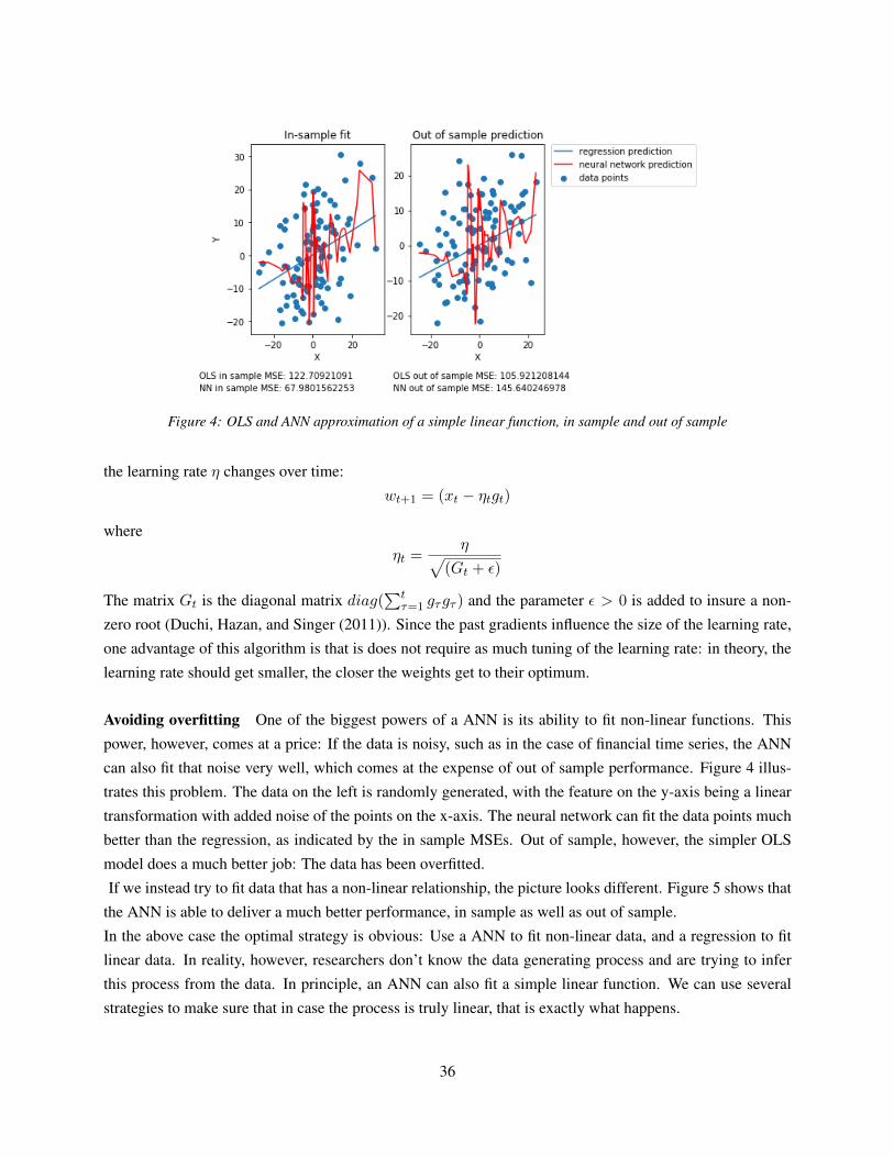
Figure 4: OLS and ANN approximation of a simple linear function, in sample and out of sample
the learning rate η changes over time:
wt+1 = (xt − ηtgt)
where
ηt =η√
(Gt + ε)
The matrix Gt is the diagonal matrix diag(∑t
τ=1 gτgτ ) and the parameter ε > 0 is added to insure a non-
zero root (Duchi, Hazan, and Singer (2011)). Since the past gradients influence the size of the learning rate,
one advantage of this algorithm is that is does not require as much tuning of the learning rate: in theory, the
learning rate should get smaller, the closer the weights get to their optimum.
Avoiding overfitting One of the biggest powers of a ANN is its ability to fit non-linear functions. This
power, however, comes at a price: If the data is noisy, such as in the case of financial time series, the ANN
can also fit that noise very well, which comes at the expense of out of sample performance. Figure 4 illus-
trates this problem. The data on the left is randomly generated, with the feature on the y-axis being a linear
transformation with added noise of the points on the x-axis. The neural network can fit the data points much
better than the regression, as indicated by the in sample MSEs. Out of sample, however, the simpler OLS
model does a much better job: The data has been overfitted.
If we instead try to fit data that has a non-linear relationship, the picture looks different. Figure 5 shows that
the ANN is able to deliver a much better performance, in sample as well as out of sample.
In the above case the optimal strategy is obvious: Use a ANN to fit non-linear data, and a regression to fit
linear data. In reality, however, researchers don’t know the data generating process and are trying to infer
this process from the data. In principle, an ANN can also fit a simple linear function. We can use several
strategies to make sure that in case the process is truly linear, that is exactly what happens.
36

Figure 5: OLS and ANN approximation of a non-linear function, in sample and out of sample
Early stopping The first strategy we introduce is early stopping. What we usually care about in train-
ing a model is its out of sample performance. Since we know that we can fit the data perfectly if we make the
model big enough and train it long enough Winkler and Le (2017), we want to make sure we stop fitting the
data at the right point in time. What we need in order to do that is to evaluate its out of sample performance
during the training process in order to stop at the right point in time.
When training a model, the data is usually split into two parts: A training dataset and a test dataset. The
training set is used to optimize the model and fit it to the data, whereas the test dataset is used to evaluate the
predictive performance of the model. In order to ensure the reliability of that test, it is imperative that the
test data cannot be used in the training process.
In order to have a ”mock” out of sample test during the training process, the training set is split into two
datasets. The third dataset is called the validation set and is used to determine when to stop the model train-
ing process. Usually, the when the model’s performance on the validation set stops improving, the training
process is stopped.
Regularization Technically, early stopping can be considered a strategy in the broader category of
regularization. As mentioned in the opening section, the size of the weights is a relatively bigger determinant
of model complexity than the number of nodes and layers. A thought example can help to informally give
an idea of why this is the case for an ANN with sigmoidal activation. Consider the logistic curve in Figure
6. The curve is described by the following equation
zi =1
1 + e−w>i xi
37
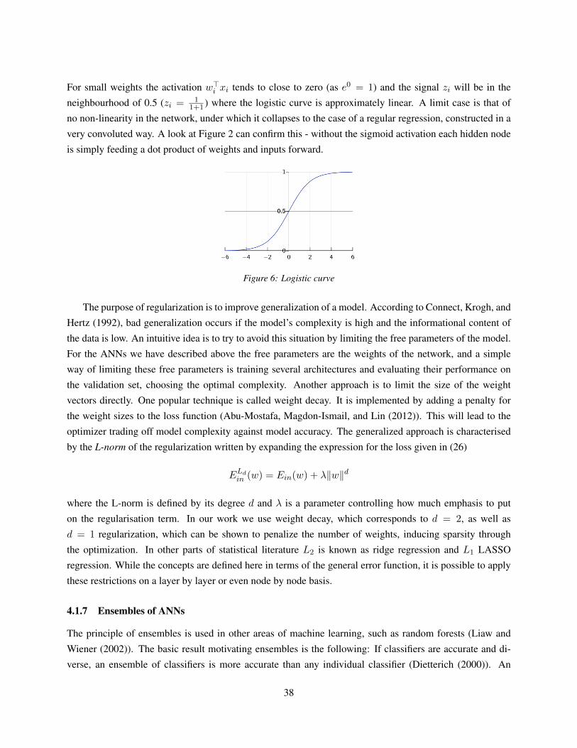
For small weights the activation w>i xi tends to close to zero (as e0 = 1) and the signal zi will be in the
neighbourhood of 0.5 (zi = 11+1 ) where the logistic curve is approximately linear. A limit case is that of
no non-linearity in the network, under which it collapses to the case of a regular regression, constructed in a
very convoluted way. A look at Figure 2 can confirm this - without the sigmoid activation each hidden node
is simply feeding a dot product of weights and inputs forward.
Figure 6: Logistic curve
The purpose of regularization is to improve generalization of a model. According to Connect, Krogh, and
Hertz (1992), bad generalization occurs if the model’s complexity is high and the informational content of
the data is low. An intuitive idea is to try to avoid this situation by limiting the free parameters of the model.
For the ANNs we have described above the free parameters are the weights of the network, and a simple
way of limiting these free parameters is training several architectures and evaluating their performance on
the validation set, choosing the optimal complexity. Another approach is to limit the size of the weight
vectors directly. One popular technique is called weight decay. It is implemented by adding a penalty for
the weight sizes to the loss function (Abu-Mostafa, Magdon-Ismail, and Lin (2012)). This will lead to the
optimizer trading off model complexity against model accuracy. The generalized approach is characterised
by the L-norm of the regularization written by expanding the expression for the loss given in (26)
ELdin (w) = Ein(w) + λ‖w‖d
where the L-norm is defined by its degree d and λ is a parameter controlling how much emphasis to put
on the regularisation term. In our work we use weight decay, which corresponds to d = 2, as well as
d = 1 regularization, which can be shown to penalize the number of weights, inducing sparsity through
the optimization. In other parts of statistical literature L2 is known as ridge regression and L1 LASSO
regression. While the concepts are defined here in terms of the general error function, it is possible to apply
these restrictions on a layer by layer or even node by node basis.
4.1.7 Ensembles of ANNs
The principle of ensembles is used in other areas of machine learning, such as random forests (Liaw and
Wiener (2002)). The basic result motivating ensembles is the following: If classifiers are accurate and di-
verse, an ensemble of classifiers is more accurate than any individual classifier (Dietterich (2000)). An
38

accurate classifier is one that is better than a random guess. Diverse classifiers make errors that are not corre-
lated. Even though errors are likely not completely uncorrelated in our case, local minima in the error surface
and elements of randomness introduced in the training procedure can make ensembles of ANNs generalize
better than individual ANNs (Hansen and Salamon (1990)).
Our learning problem is a regression problem, which is characterized by a real-valued rather than discrete
target. Motivated by above results and for the simple purpose of summarizing model predictions we adopt
the ensemble idea by letting different ANNs vote about a prediction. In practice, this vote is a simple average
of the predictions.
4.2 Principal Component analysis
In Vidal, Ma, and Sastry (2016), Principal component analysis (PCA) is defined as ”the problem of fitting
a low-dimensional affine subspace S of dimension D � d to a set of points {x1, x2, ..., xN} in a high-
dimensional space RD.” It is a commonly used dimensionality reduction technique that relies on projecting
data into the dimensions preserving the maximal variance.
The idea behind principal component analysis is that observed data with D features can be transformed
into a dataset with d � D features while preserving most of the information in the data. The reason why
this is possible is linear correlation between different features: (parts of) some features are ”unnecessary”
from an informational perspective due to linear correlation between features.
As it turns out, the principal components of a random variable can be computed using the Eigenvalues
and Eigenvectors of that random variable’s covariance matrix. We will proof this result in the following and
follow the proof described in Vidal, Ma, and Sastry (2016).
The d principal components of a random variable z (in a special case with zero mean, but the same result
applies with a non-zero mean) are defined as
xi = uTi z ∈ R, ui ∈ RD, i = 1, 2, 3, ..., d
the vectors ui are picked in such a way that the variance of xi is maximized subject to uTi ui = 1, and the
d principal components are ordered by descending variance. The maximization problem to find the first
principal component is:
maxu1∈RDuT1 Σzu1s.t.uT1 u1 = 1
because V ar(uT z) = E[(uTx)2] = E[uTxxTu] = uTΣzu. We can form a Lagrangian to get the following:
LuT1 Σzu1 + λ1(1− uT1 u1)
39

with the optimality condition:
Σzu1 = λ1u1 and uT1 u1 = 1
To find the second principal component, we start by noting that the two principal components need to be
uncorrelated. That also implies, as described in Vidal, Ma, and Sastry (2016), that u2 and u1 have to be
orthogonal. Including this as a constraint into the optimization problem, and solving the Lagrangian, we get
the following optimality condition:
Σzu2 +γ
2u1 = λ2u2 , uT2 u2 = 1 and uT1 u2 = 0
here, γ is the Lagrange multiplier for the second constraint, that principal components need to be uncorre-
lated. Taking the first optimality condition and premultiplying uT1 yields that the Lagrange multiplier γ will
be 0 and the extremum value of that optimization will be:
u2Σ2u2 = λ2 = V ar(y2)
The result implies that every additional Eigenvector will be associated with the largest Eigenvalue, such
that the Eigenvector is orthogonal to all previous Eigenvectors. The nth principal component of a random
variable is thus the product of the variable with the Eigenvector associated with the nth largest Eigenvalue
of that random variable’s Covariance matrix.
4.3 Finite differences method: basis and extension for ANNs
4.3.1 Forward, backward, and central differences
As can be confirmed by any calculus textbook (see Strang (1991) chapter 2) the definition of a derivative of
a function f(t) is the limit of the difference quotient when the increment goes to zero
f ′(t) = lim∆t→0
f(t+ ∆t)− f(t)
∆t(27)
One way to think of the finite difference quotient is as an approximation for this expression where ∆t is a
’small’ number (as opposed to an infinitesimally small number). While this informal interpretation of the
finite quotient has intuitive appeal, a more rigorous definition can be derived from a Taylor series expansion
around a point t:
f(t+ ∆t) =∞∑n=0
f (n)(t)
n!(t− (t+ ∆t))n =
∞∑n=0
f (n)(t)
n!(∆t)n
= f(t) + f ′(t)∆t+f ′′(t)
2!(∆t)2 + . . . (28)
where n indicates the order of the derivative as in f (2) = f ′′ and f (0) = f .
40

Dividing through by ∆t and solving for f ′(t)
f ′(t) =f(t+ ∆t)
∆t− f(t)
∆t− f ′′(t)
2!∆t− . . .
Introducing big O notation on the right hand side with the limiting behaviour being ∆t→ 0, the largest term
is ∆t as
∆t� 1 =⇒ ∆t > (∆t)i ∀i > 1
and so we have
f ′(t) ≈ f(t+ ∆t)− f(t)
∆t+O(∆t) (29)
where the big O represents the error which is at most of magnitude: some constant times |∆t|.
Approximation (29) is the forward difference, a naming convention which is quite natural if we let t de-
note time and consider ∆t a positive time step. Another possible approximation of the first derivative is the
backwards difference:
f ′(t) ≈ f(t)− f(t−∆t)
∆t+O(∆t) (30)
Because the increment is now negative the Taylor series, which can be truncated to approximation (30),
includes a (−∆t)n factor which leads to a sequence of consecutive positive and negative terms
∞∑n=0
f (n)(t)
n!(−∆t)n = f(t)− f ′(t)∆t+
f ′′(t)
2!(∆t)2 − f ′′′(t)
3!(∆t)3 + . . . (31)
This is where the effort of arriving at (29) by (28) rather than conjecturing it from (27) pays off; by subtracting
(31) from (28) we can form a new series where the f ′′(t)2! (∆t)2 cancels out, which after rearranging similar
to the steps above leads to the what is known as the central difference approximation:
f ′(t) ≈ f(t+ ∆t)− f(t−∆t)
2∆t+O
((∆t)2
)(32)
Recalling that the big O we consider is for ∆t → 0 the square in big O of (32) guarantees a more tightly
bound error than the forward and backward differences. For this reason we choose the finite central differ-
ence is our candidate for calculating numerical derivatives in our analysis of the neural ANNs we train.
Furthermore, by adding (29) and (30) we can obtain the second central difference approximation of f
f(t+ ∆t) + f(t−∆t) = f(t) + f(t) + f ′(t)∆t− f ′(t)∆t+f ′′(t)
2(∆t)2 +
f ′′(t)
2(∆t)2 + . . .
f(t+ ∆t) + f(t−∆t)
(∆t)2=
2f(t)
(∆t)2+ 2
f ′′(t)
2+ . . .
41

f ′′(t) =f(t+ ∆t) + f(t−∆t)− 2f(t)
(∆t)2+O
((∆t)2
)(33)
For non-linear systems high-order derivatives are naturally of interest for interpretation. Through similar
derivations it is also possible to obtain the central difference approximation to the cross-derivative.
∂2f(x1, x2)
∂x1∂x2=f(x1 + ∆, x2 + ∆)− f(x1 + ∆, x2 −∆)− f(x1 −∆, x2 + ∆) + f(x1 −∆, x2 −∆)
4(∆)2+O
((∆)2
)Exchanging x for t as the symbol for an independent variable, and dropping the t in ∆t to emphasis the
generality of the increment.
4.3.2 Extension: The non-linearity score RMSDL
The applications of these numerical derivatives to ANNs is theoretically justified by the heavy dependence
on the chain-rule in the training of these models. To train by gradient descent it is imperative to choose acti-
vation functions that are differentiable, which justifies the Taylor expansion in e.g. (28). In our study, a main
interest is quantifying non-linearities to understand how important such features are for making predictions.
Both the second order and cross difference approximation contains information about such non-linearities,
as they are zero for linear relations, which can easily be seen from (33)5. In practice, these higher order
approximations unfortunately turn out numerically unstable when applied to the our ANNs. Some errors are
expected for numerical methods, but in testing our implementation on toy-models (linear and non-linear) in
comparison to our ANNs, we find a particularly worrying error. In toy-models this error clearly discerning
from expected results because it is very small (for ∆ = 1e− 3, which is a stable choice, the error is around
1e − 10), however, for ANNs these errors can be large6. Since these higher-order approximations are im-
portant to our analysis, and we do not find the level of discrete judgement required to employ them in the
context we would like acceptable, we device an extension specialised to our needs.
The essential principal of the finite difference method that we build on is the expansion around a point
of interest. In our case this point is a vector of forward rates, which are the input for predicting the excess
return one year into the future (as described in Description of forecasting approaches in our Analysis sec-
tion). Our usual notation for this vector is f t, but to not confuse this vector with the function f discussed
here, we will use xt in this context. Instead of extending the Taylor expansion to higher orders we increase
the range of the expansion by turning ∆ into a vector ∆, representing a range [−i, i]. Analogous to the first
central difference approximation we vary each element of xt individually, while holding additional values
fixed. Predictions of excess returns are calculated by adding an element form ∆ to the selected x (say xj)
and running the inputs through the ANN. To make matters slightly more concrete the i’th prediction hprx5Consider t = 1, ∆t = 0.1, and f(t) = α+ βt, it follows that f(t) = α+ β, f(t+ ∆t) = α+ β1.1, f(t−∆t) = α+ β0.9
and so the numerator of (33) becomes α+ β1.1 + α+ β0.9− 2(α+ β) = 06In one ANN model that we by construction make linear, we find errors on the magnitude of 1e− 1
42
from varying xj where j = 3 is
f(xt,∆i, j) = hprxt,j,i = hprxt,3,i = f([x1 x2 x3 x4 x5] + [0 0 ∆i 0 0]) (34)
where the function of interest f in our case is the ANN, but could be any function. As a shorthand we
write f(xj) for the predictions obtained by varying xj as described in (34) over [−i, i], which in practise is
discretized by choosing equally spaced values in the interval. To calculate the sensitivity to the de/increments
in ∆ we regress f(xj) on ∆ and estimate
f(xj)i = yi = β0 + β1∆i (35)
where β0 is the intercept and β1 is the sensitivity to the de/increments i. In the case of a linear f the
coefficients is simply
β0 = xj β1 = βxj
This is exactly the result we would get from applying the first order central difference approximation. For
a truly linear relation the estimated coefficients are the coefficients of the population model, which corre-
sponds to a big O term in (32) of O((∆t)2
)= 0. An equivalent characteristic of the truly linear case is that
all residuals are zero. The length of ∆ does not matter and we are equally well of considering just a single
de/increment, i.e. applying one of the difference approximations described above.
In general, we do not expect ANNs to produce linear predictive functions; the point of applying them is
to allow for non-linearities. However, paraphrasing a point from our section on the general ANN learning
set-up, allowing for non-linearity does not mean disallowing linearity. As we will cover below in our section
on architectures, we do try different ways of adding strictly linear components to our ANNs , but the opti-
mum may still be to let the designated non-linear parts act mainly linear in which case training will lead to
the ANN converging on such a set-up. The characteristics of the linear case in the approach outlined above
suggests a straightforward test of linearity of any function: estimate (35), calculate the residuals, and if any
residuals are non-zero strict linearity is rejected. One thing to notice here is that f is a predictive function of
a fitted model, so for regular OLS, f would describe the relationship between y and xj ; a relationship where
residuals by construction are zero. The test is, however, still very restrictive which implies that it is unlikely
to be informative on the temporal dynamics of an estimated relationship. As our analysis is essentially time-
series analysis this is a major drawback, so we turn the test into a simple distance measure, calculating the
root mean squared error from the residuals of estimating f(xj) of all the xj’s i.e.
RMSDL =1
J
∑j∈J
√1
I
∑i∈I
(f(xj)i − f(xj)i)2
43

where the abbreviation is for Root Mean Squared Distance to Linear7.
Defined this way RMSDL captures non-linearity in relationships between the dependent variable and in-
dividual independent variables, analogous to the second order difference approximation. To extend the
measure to also capture relationships akin to the cross difference approximation we extend the variations
we do of xt to include interactions. In assigning an absolute meaning to RMSDL we worry about ”double
counting” some non-linear relations this way, as varying x1 and x2 includes varying x1, which may on it’s
own have a non-linear relationship with yi. However, the main focus of our analysis is relative, considering
the dynamic behaviour of the same model over time, we are more concerned about missing information. For
this reason we include all the possible combinations of elements of xt in the RMSDL we employ in our
analysis. To clarify this point we give another concrete example like (34) this time for the interaction 1, 3, 5
f(xt,∆i, j) = hprxt,j,i = hprxt,(1,3,5),i = f([x1 x2 x3 x4 x5] + [∆i 0 ∆i 0 ∆i])
Based on the above example, it is reasonable to ask why we would bother with varying individual inputs or
combinations thereof instead of just varying all inputs at the same time. The reason is that changes in inputs
also could also cancel each other out. Coupled with the more practical consideration that these variations
are computationally inexpensive we opt for the more comprehensive definition of the measure that includes
variation of all combinations.
So far we have kept the hyper-parameter i conveniently unspecified. In practice the range to expand the
predictive function over will be a matter of the data that the model is fitting. Different visions based on
ranges of or variation in the data could be envisioned, but with the purpose of relative interpretation in mind,
we choose a pragmatic approach and test different sizes of the window. We find that for the models we
consider, the effect of changing the size of the window matters for the overall scale, but not the dynamics of
RMSDL.
4.4 Generalized degrees of freedom (GDF)
The term ”degrees of freedom” (DF) of a regression model is defined in Ye (1998) as ”the number of vari-
ables in the model”. The interpretation of this number is, in our case, straightforward. The greater the DF
of a model, the easier it can fit the distribution observed in the data. At the same time, a greater number of
DF indicate a greater degree of model flexibility, which brings about a danger of overfitting. The motivation
to use a methodology that enables us to compare DF across models is therefore to enable us to compare the
degree of possible overfitting we have in each of the models. Following Ye (1998), we will first show that
the degrees of freedom in a linear model are in fact equal to the GDF. In a second step, we will outline the
algorithm used to calculate GDF in the paper, which will also be employed in our study.
7A practical example can be found in the appendix on RMDSL.
44

We assume a standard OLS model:
Y = Xβ + ε with ε ∼ N(0, σ2I) (36)
The estimate for β is then
β = (X ′X)−1X ′X (37)
and the fitted values of Y are:
Y = X(X ′X)−1X ′Y (38)
the term in front of Y projects it onto the vector of fitted values Y and is therefore often called projection
matrix. Assuming the number of observations n is smaller than the number of features p andX has full rank,
we know that (X ′X)−1 exists. But then we also know that:
tr(X(X ′X)−1X ′) = tr(X ′X(X ′X)−1) = tr(Ip) = p (39)
This follows from the fact that the trace operator is commutative. We thus know that the trace of the projec-
tion matrix is equal to the degrees of freedom of the regression model. Since the hat matrix transforms the
observed values into fitted values, we can reexpress its trace as:
p = tr(H) =∑i
hii =∑i
∂yi∂yi
(40)
The above is the definition of generalized degrees of freedom for linear regression models. Intuitively, it
measures the flexibility of the modelling procedure. The more flexible the model, the more the fitted values
will change when the observed target changes. For simple models like the one above, calculating the partial
derivatives is analytically straightforward. For more complex models such as ANNs, however, we have to
numerically approximate the values. In practice, the GDF are calculated as follows. First, we fix a number
of permutations T . For each permutation, a vector of small changes ∆t is generated from a distribution. The
vector is added to the vector of actual observations and the model is refitted. Then, the sensitivity of that
specific fitted value to a small change in the observations is estimated with the regression model:
yi(Y + ∆t) = α+ hiδti, for t = 1, ..., T (41)
When this has been done T times, the average of the sum of the sensitivities hi equals the GDF.
4.5 Generalized method of moments (GMM) for regression
The framework of generalized method of moments (GMM) developed by Hansen (1982) is in its generality
much richer than standard error correction in linear regressions, however, it is nonetheless useful for this
purpose. Since this is the way we use GMM to replicate the results of Cochrane and Piazzesi (2005) we
45

focus exclusively on using GMM for OLS with serially correlated errors.
Moment restriction
GMM requires the econometrician to impose identifying orthogonality conditions. In more involved mod-
elling, choices amounts to economical assumptions such as expected returns discounted by marginal utility
growth (Cochrane (2009)). For OLS the regressors must be uncorrelated with the error term, which works
out to be the an exact identification in the the GMM framework (Cochrane (2009))
E[xt(yt − β>xt)] = 0
where bold font indicates (column) vectors, xt is the values of the independent variables at time t pre-
appended a 1 to include an intercept. Technically t is an indexes the rows of the X matrix in the population
equation of the familiar form
y = Xβ + ε =⇒ εt = yt − β>xt
The ’method of moment’ part of GMM is to replace moments of the population by sample counterparts
1
T
T∑t=1
[xt(yt − x>t β)] = 0 =⇒ 1
T
T∑t=1
[xtyt] =1
T
T∑t=1
[xtx>t β)]
where 1T cancels out. Now since the dimension of xt and β is [(1 + p) × 1] the dimension of xtxτt is
[(1 +p)× (1 +p)] and β does not depend on t we can post-multiply β to the sum rather than each individual
observation. If we rewrite∑T
t=1 xtxτt = X>X and
∑Tt=1[xtyt] = X>y we pre-multiply both sides by the
inverse of X>X and recognise the OLS estimator
(X>X)−1X>y = (X>X)−1X>Xβ =⇒ β = (X>X)−1X>y
In this way GMM can actually be considered a justification of OLS.
Standard errors
As indicated in the introduction, the trick of using GMM in the context of simple OLS regression is to
correct standard errors. Without going to deep into the framework the variance of the estimator is expressed
as (following Cochrane (2009)):
V ar(β) =1
Td−1Sd−1
where
d =∂{
1T
∑Tt=1[xt(yt − x>t β)]
}∂β
= X>X S =
∞∑i=−∞
E(εtxtx>t−iεt−i)
46

Where varying the assumptions on S is suggests different estimation strategies for the variance (and as such
the standard errors) of the estimator. With the assumptions of serial uncorrelated and homoscedastic mean
zero errors we have regular OLS errors as only i = 0 in S will be non-zero with the value
E(ε2t )E(xtx>t−i) = V ar(ε2t )X
>X =⇒ V ar(β) = (X>X)−1V ar(ε2t )
as X>X cancels out (X>X)−1. The framework also nests the robust White errors for heteroskedastic, but
serially uncorrelated errors. However, as the the regressions of holding period excess returns of Cochrane
and Piazzesi (2005) is done on a rolling basis (just as the original Fama and Bliss (1987) regressions) the
more appropriate form is serially correlated errors, which means that the formula for S does not simplify.
Clearly, the estimation of infinite lags is not feasible, and long-dated lags tends to be poorly estimated
(Cochrane (2009)), so in choosing the number of lags we follow the method outlined in the appendix to
Cochrane and Piazzesi (2005) and set number of lags to 12 estimating S by
S =
12∑i=−12
(1
T
T∑t=1
(εtxtx>t−iεt−i)
)
47

5 Data Description and Reproduction of Established Results
In this section, we describe and introduce the data we use. First we provide descriptive statistics then we
reproduce some earlier results in order to show if and how our data differs from datasets of earlier studies. We
cover in sample relationships as part of our descriptive section as our main focus is on out of sample results.
Our rationale for including in sample regression results is to set the scene and give the reader confidence in
our results: showing that our data behaves as expected during the periods covered in earlier papers.
5.1 Descriptive statistics
In this section, we will describe the dataset we are using and summarize the manipulations that have been
done to it. We use a bond dataset that includes log zero yields for different maturities for the period between
June 1952 and December 2015. In our analysis, we use data starting from 1962, following Cochrane and
Piazzesi (2005). The zero yields have been bootstrapped from observed bond prices. From the log-yields,
we calculate forward rates, prices and excess holding period returns. Please refer to the terminology section
for more information on how these are connected. Descriptive statistics on yields, forward rates and holding
period excess returns can be found in Table 1, Table 2 and Table 3.
The mean of the log yields increases with maturity showing the pattern of an on average upward sloping
yield curve that can be considered suggestive of a term-premia. Standard deviation decreases with maturity,
indicating that yields on the longer end of the yield curve fluctuate less then at the short end. As described
in our section on affine models there is a link between volatility and risk-premia in CIR-style models. With
decreasing volatility such a model would, however, also require term-premia to produce an upward sloping
yield curve. The minimum yield increases with maturity. The maximum does not show a similar tendency.
Plotting the yields (Figure 7) reveals another pattern. There is a strong upward trend between the start of the
period and about 1982. Afterwards, the yields trended downwards until the end of the dataset.
48
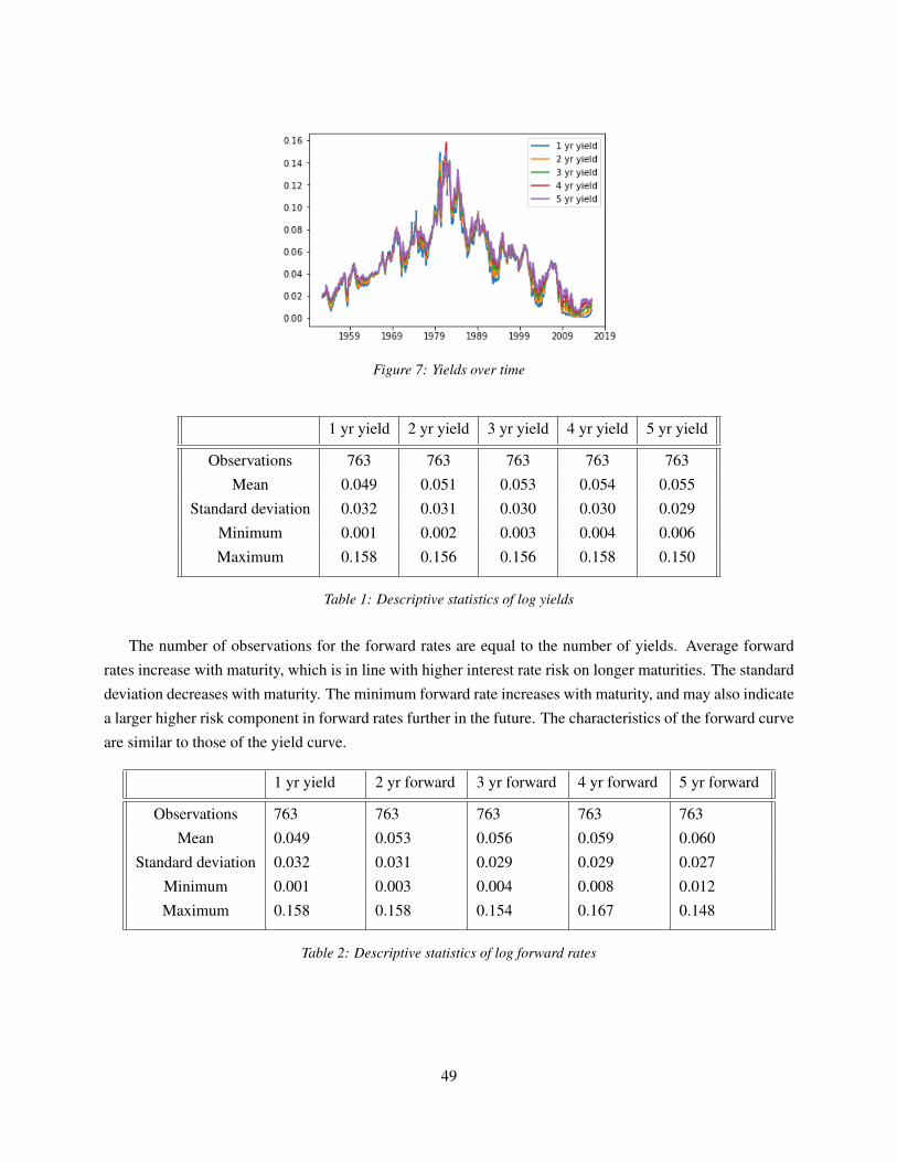
Figure 7: Yields over time
1 yr yield 2 yr yield 3 yr yield 4 yr yield 5 yr yield
Observations 763 763 763 763 763
Mean 0.049 0.051 0.053 0.054 0.055
Standard deviation 0.032 0.031 0.030 0.030 0.029
Minimum 0.001 0.002 0.003 0.004 0.006
Maximum 0.158 0.156 0.156 0.158 0.150
Table 1: Descriptive statistics of log yields
The number of observations for the forward rates are equal to the number of yields. Average forward
rates increase with maturity, which is in line with higher interest rate risk on longer maturities. The standard
deviation decreases with maturity. The minimum forward rate increases with maturity, and may also indicate
a larger higher risk component in forward rates further in the future. The characteristics of the forward curve
are similar to those of the yield curve.
1 yr yield 2 yr forward 3 yr forward 4 yr forward 5 yr forward
Observations 763 763 763 763 763
Mean 0.049 0.053 0.056 0.059 0.060
Standard deviation 0.032 0.031 0.029 0.029 0.027
Minimum 0.001 0.003 0.004 0.008 0.012
Maximum 0.158 0.158 0.154 0.167 0.148
Table 2: Descriptive statistics of log forward rates
49

2 yr→ 1 yr 3 yr→ 2 yr 4 yr→ 3 yr 5 yr→ 4 yr
Observations 751 751 751 751
Mean 0.004 0.008 0.010 0.011
Standard deviation 0.016 0.030 0.042 0.051
Minimum -0.056 -0.104 -0.135 -0.175
Maximum 0.059 0.102 0.144 0.169
Table 3: Descriptive statistics of holding period excess return data. For the holding period returns, the captions denotewhat happens to the longer maturity bond in the portfolio: ”2 yr → 1 yr” thus describes the holding period excessreturn of a 2 year bond that turns into a one year bond during the holding period.
The number of observations for the holding period return is lower than the number of forward rates,
due to the fact that the first holding period return can only be calculated for the period one year after the
time series begins. The holding period excess returns we use in our analysis are described in Table 3. The
mean holding period excess return increases with maturity. Here, the standard deviation varies a lot more
than in the previous two cases and is upward sloping. To the extend that excess returns represent realized
risk premia, this inverted relation between as compared to yields and forwards are at odds with the volatility
link in a CIR-style model explaining the dynamic behaviour risk-premia. If variations in risk-premia are
caused by variation we would expect that the most volatile excess returns are found . In contrast to yields
and forward rates minimum excess returns are all negative. This is in line with a risk-premium explanation
of excess returns requiring that loses are possible. From the extremes of minimum and maximum, upsided
and downside seems symmetrical, however, the small, but positive average excess returns for all maturities
are reasonable for risk premia that are at least on average positive.
Furthermore, we use a time series of 68 macroeconomic indicators. This dataset differs from the one used
in Ludvigson and Ng (2009) mainly due to the fact that the variables are observable in real time. Ghysels,
Horan, and Moench (2014) point out that Ludvigson and Ng (2009) do not use real time data, which is prob-
lematic for what we intend to do in this thesis. We therefore use a dataset that contains only information that
would have been available to an investor in real time. Reporting summary statistics of 68 variables is not
very convenient. We therefore take the first ten principal components of the macroeconomic dataset before
showing summary statistics. The Eigenspectrum, showing which principal components contain how much
of the total variance in the data, are depicted in Figure 8. We have 407 observations for the macroeconomic
data. The data is available for the period between February 1982 and December 2015. To illustrate the
ordering of principal components, Figure 9 shows the first five principal components over time. The plot
shows the effect of PCA: The first principal component has the largest variance, the second one the second
largest etc. It also shows that the variance seems to increase over time.
50

Figure 8: Eigenspectrum of real time macroeconomic dataset
Figure 9: Plot of macroeconomic dataset
5.2 Reproduction of Cochrane Piazzesi in sample results and combination with macroeco-nomic data
We run some of the regressions similar to the ones ran in Cochrane and Piazzesi (2005) and inspired by
Ludvigson and Ng (2009) in order to compare our data to what they used. First, we ran the regression of
five forward rates on the average excess return. We find a tent shaped pattern with similar coefficients and
standard errors (GMM corrected) and an R2 of 0.346, which corresponds closely to the results for the same
regression in Cochrane and Piazzesi (2005). Figure 10 shows the typical tent shape found in Cochrane and
Piazzesi (2005). The coefficients, GMM corrected standard errors and t-statistics are shown in Table 4.
T-statistics drop for almost all forward rates in moving from the CP period to the the full sample.
51

Intercept 1-year
yield
2-year
forward
rate
3-year
forward
rate
4-year
forward
rate
5-year
forward
rate
CP
sample
Coefficients -0.032 -2.056 0.702 2.96 0.813 -2.017
Standard er-
ror
0.014 0.367 0.720 0.552 0.479 0.43
t-stat -2.34 -5.61 0.97 5.36 1.7 -4.69
Full
sample
Coefficients -0.015 -1.279 -0.575 1.723 1.364 -1.023
Standard er-
ror
0.010 0.428 0.594 0.786 0.434 0.494
t-stat -1.558 -2.986 -0.967 2.191 3.146 -2.070
Table 4: Coefficients, standard errors and t-statistics for Cochrane-Piazzesi sample period and our full sample. Stan-dard errors are corrected using GMM with 12 lags, as described in the Methodology section
Figure 10: Tent for same period as in Cochrane and Piazzesi (2005) and for our sample period
Next, we run the same regression on our full sample. We find a less pronounced tent shape and a much
lower R2 of 0.2285, indicating that there might be changes from one period to another. Figure 11 confirms
that suspicion and shows that especially from the 30 year period starting from about 1980, the tent shaped
pattern breaks down. For a 20 year sample period, we see the tent break down already from 2000.
52

Figure 11: 20 and 30 year rolling CP regression coefficients
Concluding on our comparison with the Cochrane and Piazzesi (2005) data, we believe that we have a
comparable dataset which reproduces the results of the original paper for the corresponding sample. We find
that including more periods changes the predictability using forward rates for the worse and results in the
pattern of coefficients changing slightly. The plot of CP regression coefficients on a 30 year basis in Figure
11 shows how stable the relationship discovered in the original paper was at that time and how it has changed
since. We include the plot of a 20 year rolling window as well, as it corresponds to the window we focus on
for larger parts of our analysis. The coefficients are slightly more volatility on this basis, but overall exhibits
the same pattern of a stable ranking that breaks down in recent years.
We rerun the in sample regression first for the forwards and excess returns exclusively, and then include
the real time macroeconomic data. We find that the explanatory power of the forward rates on excess returns
is much lower during the period for which we have macroeconomic data. We find an R2 of 0.154 for that
regression. Once including the macroeconomic data, we find an R2 of 0.198. The adjusted R2 increases
by 0.033 when including the real time macroeconomic data. When including more principal components
we can get a higher R2, at the expense of adjusted R2. We conclude from this that the real time macroeco-
nomic data adds some predictability in sample, but not as much as was found in Ludvigson and Ng (2009).
The t-statistics for most of the principal components are furthermore very low, indicating that they are not
significant. The drop in added predictive performance compared to Ludvigson and Ng (2009) when using
real-time macroeconomic data rather that revised data is in line with the findings in Ghysels, Horan, and
Moench (2014).
6 Methodology
This part of the thesis focusses on the analytical approach we take in investigating bond predictability. In
previous sections we have introduced a number of papers from the empirical bond pricing literature and
summarized methods and results from these papers. We want to update the findings of these papers and use
their predictive performance as a benchmark for our ANN models. We first introduce the methods we use to
rate performance statistically and economically, and provide justification for our choices.
53

6.1 Statistical measures to rate out of sample performance
Testing how well a model does out of sample has some major advantages. If we train a model on past data
and manage to predict future realizations of the variables, the model we have trained reflects the true data
generating process. When using models as involved and powerful as deep ANNs, out of sample performance
is the only measure that can truly evaluate the model. That is due to the fact that ANNs with enough
degrees of freedom can essentially fit any dataset as mentioned before (Winkler and Le (2017)), which of
course includes noise in the training data. Our choice of out of sample performance as the criterion for
model evaluation is thus without alternative. The models we use as benchmarks, namely Cochrane and
Piazzesi (2005) and a model inspired by Ludvigson and Ng (2009), use the in sample R2 as a measure of
performance. The in sample R2 over a period from t = 0 to T is calculated as follows:
R2IS = 1−
∑t(yt − yt)2∑t(yt − y)2
y =1
T
∑t
yt (42)
The intuitive interpretation of this measure is essentially the percentage of the variation in the target variable
that is explained by the prediction. In the case of out of sample performance, however, using the same
measure could be considered an unfair comparison. The reason for this is that the value y is not known when
the prediction is made. We thus follow Campbell and Thompson (2008) in their approach and use an R2 that
can be compared to its in sample counterpart:
R2OS = 1−
∑t(yt − yt)2∑t(yt − y∗)
y∗ =1
S
∑s
y0−s (43)
The average y∗ is the average value over the training period which ends at t = 0. A negative R2OS indicates
that a simple unconditional expectation (i.e. the mean over the training period) is a better prediction of the
test data. This could be due to several reasons. Over-fitting is a main concern, as well as spurious relations
in the data as both conclusions would invalidate the relationship discovered in sample. A less damning
explanation may be a noisy data-generating process. Campbell and Thompson (2008) argue that if the true
data generating process is
yt+1 = α+ βxt + εt+1 (44)
with β 6= 0, the historical average is a biased estimator. Given a small sample size and a small value for β,
the historical average may still perform better out of sample as it is more robust to noise. As we shall see this
concern comes up in relation to the out of sample performance of both our benchmarks and the algorithms
we introduce.
To separate the discussion of absolute performance from the discussion of relative performance, we gen-
erally use the root mean squared error to rank out of sample results. The root mean squared error has an
interpretation similar to a standard deviation with the conditional expectation replacing the unconditional
54

expectation
RMSE =
√√√√ 1
T
T∑t=0
(yt − yt)2 std(Y ) =
√√√√ 1
T − d
T∑t=0
(yt − y)2
where d are the degrees of freedom of a model, which for the mean (a very parsimonious model) is 1 and for
the RMSE could be taken into account by adjusting the 1T by 1
−d . In practice this is not a usual approach,
and rather than adjusting the measure directly, we consider the impact of the degrees of freedom of the
different models explicitly in our analysis.
6.2 Economic measures to rate out of sample performance
The problem of predicting excess bond returns is a regression, meaning that the target is real-valued and not
a discrete class. The statistical measures we introduced above essentially punish any deviation of the predic-
tion from the target value based on how far away it is from that value. Scoring the predictive performance
based on this measure is certainly informative, as it can tell us how well the model can produce predictions
close to the realized values of the data generating process (RMSE) and whether an unconditional expectation
can beat our model (R2OS).
From an economic point of view though, both RMSE and R2OS miss an important point. We consider an
investor that wants to know whether to go long or short the strategy of buying a longer maturity bond while
shorting a one year bond. That investor is much more interested in getting the sign of the excess return right
than predicting the value very accurately. The prediction could essentially overshoot the true value every
time, but could still deliver a much higher economic value than a prediction that is closer to the true value
but gets the sign wrong most of the time.
We thus put ourselves into the shoes of an investor that uses our different predictors as a trading signal.
We will use the signal in two different ways. First, we have a strategy in which a positive predicted excess
return triggers a long position, and a negative predicted excess return triggers a short position. We use the
Sharpe ratio (SR) introduced in Sharpe (1994) to measure the performance of the trading strategies resulting
from the different signals. We compute the annualized SR as follows:
SRann =rannt
σannt
(45)
We use annualized values, which implies that the numerator is calculated as follows:
rannt =1
T
T∑t=1
rmt (46)
55

The values in the brackets are the monthly returns of our strategy. Since the investment period of the strategy
is one year, the returns are already annualized. Also, we use the returns of the strategy as excess returns
since we assume that we finance the investment in the longer maturity bond at the one-year yield, which we
decided to treat as a risk-free rate in the context of calculating the SR. The volatility is then calculated as:
σannt =
√√√√ 1
T
T∑t=1
[rmt − rannt ]2 (47)
The SR thus measures how well an investor is compensated for the risk they take and gives a good indication
of the value of the signal. Notice that we calculate the ex-post SR, and not the ex-ante version. This difference
is important, since the backward looking version of the ratio downplays some of the risk an investor faces in
real-time.
6.3 Description of forecasting approaches
In this section we explain our learning set up closer. We do this for each of the benchmarks individually and
as a last step explain how we train different ANNs and use them to predict excess returns.
6.3.1 Unconditional expectation
In order to check the value of our results, we compare our predictions to the unconditional expectation of
excess returns. That unconditional expectation is a simple moving average of past excess returns:
E[rx
(n)t+1
]=
t∑k=t−s
rx(n)k
The purpose of including the unconditional expectation is to sanity check the value of the more complicated
models we are using. If we do not manage to do better than the unconditional forecast out of sample, that
raises questions regarding the data generating process that we introduced in our discussions of performance
measures.
6.3.2 Cochrane-Piazzesi approach
Our first benchmark is the approach used in Cochrane and Piazzesi (2005) (CP). The authors run restricted
and unrestricted regressions of holding period excess returns on forward rates. We use the unrestricted re-
gressions because they have a higher R2IS and we want to compare our set up against the best benchmark
possible. This is also why we include lags, in order to test whether it is the additional information or the
model that explains a possible difference in predictive power.
56

We train the model on a training dataset. For linear regression, minimizing squared error has an analytical
solution so the term training may seem peculiar, but conceptually the process of choosing model parameters
is the same step in the process regardless of the optimization method applied. Since the model selection
is done beforehand, we do not need a validation dataset. The time index t indicates the year that data is
observed at. Excess returns are observed one year after the forward rates are observed. For sample length S
at time t, we regress the expected excess return across four maturities n from the period of t− s to t (today),
on the vector of forward rates f from the period one year before, i.e. form t − s − 1 to t − 1. From this
regression we get αt and vector βt, which fulfils the following Sn equations minimizing the squared error
ε2:
rx(n)t−s = α
(n)t + β
(n)t f t−s−1 + ε
(n)t−s ∀ s ∈ [0, S), n ∈ [1, 4]
where
E[ε|f ] = 0
which corresponds to the unrestricted model in Cochrane and Piazzesi (2005). Making the prediction of the
excess returns one year from now (at time t+ 1) leads to the following:
E[rx
(n)t+1|f
]= α
(n)t + β
(n)t f t
Following this approach yields a time series of predictions that we subsequently compare to the observed
values and score using the metrics described above.
6.3.3 Cochrane-Piazzesi approach using real time macroeconomic data
Similar to Cochrane and Piazzesi (2005), Ludvigson and Ng (2009) use a linear regression model to fit ob-
served values one year before to excess holding period returns one year later. The authors use forward rates
and a number of macroeconomic indicators, that they reduce in dimensionality using PCA. The in sample
approach used in Ludvigson and Ng (2009) has a few drawbacks when transferred to out of sample analysis
that we address in our implementation. First, doing PCA of the whole dataset does not work in out of sample
analysis. An investor doing a regression at time t can only transform the data using a Covariance matrix that
is known at that time. Furthermore, the authors do a grid search of which principal components and their
polynomials to include in the regression. We assume an investor chooses a share of the macro data’s variance
that they want to explain. We set this number to 95%. They will then include all these principal components
in the regression. The dataset used in Ludvigson and Ng (2009) furthermore differs from the dataset we
consider in the fact that our data was available to investors in real time while Ludvigson and Ng (2009) use
revised data. Thus the approach we use is only inspired by Ludvigson and Ng (2009) and does not exactly
reproduce their approach.
57

In practice, we start with taking realizations of K macroeconomic variables over a period t − s − 1 to
period t, which is the present year. We then take the first k principal components of that dataset. After
reducing the dimensionality to k, we run the following regression: For sample length S at time t, we regress
the expected excess return across 4 maturities n from the period of t−s to t (today), on the vector of forward
rates f from the period one year before, i.e. form t− s− 1 to t− 1 and a vector of macroeconomic variables
m for the same period. From this regression we get αt and the vectors βt and γt, which fulfils the following
Sn equations minimizing the squared error ε2:
rx(n)t−s = α
(n)t + β
(n)t f t−s−1 + γ
(n)t mt−s−1 + ε
(n)t−s ∀ s ∈ [0, S), n ∈ [1, 4]
where
E[ε|f ,m] = 0
which corresponds loosely to the model used in Ludvigson and Ng (2009). We decided to include both
macroeconomic data and
forward rates, as we are interested in the explanatory power the macroeconomic data has conditional on the
forward rates. The prediction at time t is:
E[rx
(n)t+1|f ,m
]= α
(n)t + β
(n)t f t + γ
(n)t mt
The vector of predictions is then compared to the other predictions using the same metrics as explained
before.
6.3.4 ANN architectures
According to Neuneier and Zimmermann (2012), the often repeated statement that a three-layer feed for-
ward ANN can fit any structure in the data leads to the common misconception that the characteristics of the
underlying data alone determine the quality of the resulting model. Neuneier and Zimmermann (2012) argue
that, especially for data with a low signal to noise ratio, the model building process and training process are
of high importance and play a big role in determining success or failure of the modelling process. As men-
tioned in our section on performance measures, Campbell and Thompson (2008) raise a similar concern. The
context they discuss is that of estimating the equity premium: beating the historical mean in terms of predic-
tive power is inherently difficult because of noise in the data. We operate under the assumption that our data
suffers from the same issue. We recognize furthermore that training a more advanced model on noisy data
amplifies the problem. Even if we manage to eliminate some more bias compared to the linear model noise
in the estimate might more than offset the gain from reducing the bias (Campbell and Thompson (2008)).
58

On the other hand, we want to build meaningful models. Using a model that has no interpretability and fails
to reveal anything new about the data generating process even if it is successful, is not very valuable in the
context of asset pricing. We therefore work to satisfy different constraints in model building: we want to
build intuitive models that are not too prone to overfitting, yet are able to capture non-linear relationships
and reveal something about their nature.
In order to respect these constraints, we test several models with increasingly more freedom in fitting the
data. We start from the assumption that a linear combination of five forward rates determines excess holding
period returns to a certain degree (Cochrane and Piazzesi (2005)). The CP model is thus our base-case, and
the most restricted model we try out. The other extreme is an unrestricted feed forward ANN. The last, and
most extreme case is of course the most powerful when it comes to fitting the in sample data, but on the other
hand prone to overfitting.
Figure 12: General setup of four architectures used in analysis
59

Base architecture The general structure of our models is depicted in Figure 12. The input vectors f t depict
forward rates for maturities one to five and their respective lags. The output vector hprxt+1 is a vector of
one year excess holding period returns for 2-year to 5-year bonds. Each of the models can generally be
separated into a strictly linear part and a part that allows non-linear relations. The linear part is characterized
by a linear activation function. In the non-linear enabled parts, we have three different activation functions.
First we have tanh:
f(s) = tanh(s) =es − e−s
es + e−s(48)
which has the typical s-shaped pattern of a smooth activation function and produces outputs between zero
and one. The second activation function we use is the standard sigmoidal activation:
f(s) =1
1 + e−s(49)
The sigmoidal activation is also smooth and between zero and one. The function is not as steep as the tanh
activation, which we find in individual tests produces more restricted outputs. The third activation we use is
the ReLu activation:
f(s) = max(0, s) (50)
The descriptions of the activations are taken from Heaton, Polson, and Witte (2016). The result for recurrent
neural networks described in Hochreiter (1998) about vanishing gradients - the problem that gradients die
out in deep ANNs - extends to feed forward ANNs and can be mitigated by using a ReLu activation function,
which on its linear part above zero does not die out.
We use this architecture for reasons related to the theory on bond predictability: as explained in more detail
in the theoretical part of the literature review, there might exist a ”hidden” factor, which we hypothesize to
be a non-linear combination of forward rates. Therefore most of our models are set up to facilitate training
into such a separate linear and a non-linear part.
To illustrate the relationship between the simple CP model and our setup, imagine all weights connect-
ing the non-linear part and the input to be set to zero in Figure 12. Then, the model simplifies to the CP
model, which is a weighted sum of forward rates plus a bias term that predict holding period excess returns.
The architectures we introduce in the following are summarized in Table 5.
Fixed model The first one of our models we would like to introduce, we call the ”fixed model”. The fixed
model is characterized by the weights of the linear part not being trained, but instead they are set to the
weights of the CP model. The weights on the output of the linear part (in the prediction layer) are part of the
optimization process. This implies that the ANN will be able to make each holding period excess return a
weighted sum of CP predictions and the transformations of the forward rates from the non-linearly enabled
part of the model.
60

Linear restricted model Our second model is ”linear restricted”. In this model, the weights of the linear
part of the model are part of the optimization, but they are restricted to produce only one output that must
be used in the process of predicting the different maturities of excess returns. They could end up reflecting
the tent-shaped CP factor, but could also look entirely different. The connection to the CP model is here that
Cochrane and Piazzesi (2005) describe a single factor to predict excess returns for bonds of all maturities.
By placing this linear restriction, we force the ANN to summarize the strictly linear combinations of forward
rates into a single factor.
Non-linear restricted model We call our third model ”non-linear restricted”. As the name suggests, we
place a restriction on the non-linear part of the model. Similar to the linear restriction, each of the outputs of
the three different non-linear activations are forced into a single output. In this way, the model is restricted
to make the final output a weighted sum of a strictly linear part and the individual non-linearly enabled parts.
This is instead of mixing a wider range of outputs from the latter. What we wish to achieve is a situation
where the tanh, sigmoid, and relu parts act as embedded sub-ANNs. Thus a more clean cut choice, treating
each part as an individual factor, is enforced. The interest is then to interpret the characteristics and relative
importance of each of the three.
Unrestricted model The last version, as mentioned earlier, has no restrictions placed upon it. We call it
”unrestricted model”. The general architecture is similar, but we make versions both with and without the
strictly linear part; the non-linearly enabled parts with the three different activation functions are the same.
The term we use for a strictly linear part in an ANN architecture is skip-layer. If this option is implemented,
the ANN can ”skip” the non-linear parts of the ANN by using the linear part of the architecture. In Figure
12, no ”skip-layer” option would thus imply that all weights connecting the input nodes and the linear part
of the ANN would be set to zero. Overall, it only makes sense to consider this an option in the unrestricted
models; both the fixed model and the linear restricted model would not be fixed models or linear restricted
models without the strictly linear part, and preliminary experiments suggests that the non-linear restricted
model without skip-layer is too restricted. With skip-layer, the unrestricted model is the most flexible model
and may as such be considered in the biggest danger of over-fitting.
Finally we differentiate the ANNs by size of the non-linear part. When we talk about a ”wide” model,
the non-linear parts of the the model have two hidden layers with 20 neurons each. When we say ”deep”
model, we refer to the linear part having four hidden layers with five neurons each. By ”small” model, we
mean that the non-linear parts of the architecture have two hidden layers with three nodes each.
61

CP model Fixed Linear
restricted
Non-linear
restricted
Unrestricted
Weights into linear
part
CP weights CP weights Optimized
with ANN
Optimized
with ANN
Optimized
with ANN
Output units of lin-
ear part
4 4 1 4 4
Output units of
non-linear parts
0 5(×3) for
deep
5(×3) for
deep
5(×3) for
deep
5(×3) for
deep
0 20(×3) for
wide
20(×3) for
wide
20(×3) for
wide
20(×3) for
wide
3(×3) for
small
Table 5: Overview of different architectures
6.3.5 Sample periods and training time
We consider two distinct sample periods. The first one starts in 1982 and extends to 2015, reflecting the
time for which we have macroeconomic data. We discuss performance of the predictors using a 10 year
training period extensively and only touch upon the results of a 20 year training period. The reason is that
training on 20 years of data reduces the window on which we can measure performance to only 10 years.
The second sample period we consider starts with the beginning of the dataset considered in Cochrane and
Piazzesi (2005) and extends to the end of 2015. We cannot consider predictors using macroeconomic data
for that period since our macroeconomic dataset starts in 1983. We consider both 10 year training periods
and 20 year training periods extensively due to the longer sample length. With regards to training time, we
save two versions of the ANNs during training. We did this due to the fact that early experiments indicated
only 15-25 training epochs to be optimal. We saved an additional version with 50% higher training time
in case our earlier experiments were not representative. Performance measures, however, indicated shorter
training time to be optimal.
7 Analysis and Discussion of results
7.1 Results of statistical tests
7.1.1 Benchmark performance
As mentioned before, we consider several different time windows and the performance of a rolling predic-
tion. Since the macroeconomic data we use is not available for the whole period but only starts in 1983,
we compare the unconditional mean, the CP predictor by itself, the CP predictor with lags and the same
62

combinations for the macroeconomic data for that period. For the full sample, we only use the unconditional
mean, CP and CP with lags.
Period for which we have macroeconomic data We restrict ourselves to reporting in sample R2 and out
of sample RMSE, since we are comparing ANN performance to ordinary least squares regression perfor-
mance. A rolling regression is reported in Table 6. The R2 for all predictors rises with the maturity of the
bonds for which we are trying to predict holding period excess returns. Looking at R2 as a mathematical
relationship rather than a concept, that can only mean one of two things. Either the sum of squared residuals
decreases, which would imply a smaller error made by the model, or the total sum of squares rises. We know
from Table 3 that the volatility of holding period excess returns rises with maturity. We thus know that the
total sum of squares rises as well, which implies that the sum of squared residuals rises less. There are two
possible explanations for this: Either the signal explains more of the movement for longer maturity bonds or
the model can simply fit more volatility than a simple mean which translates into a higher R2 if the target is
noisier8. We see the same tendency in a vertical direction as well: As the number of features in the model
increases, R2 rises. Again, this could be a mechanical relationship due to the models having larger degrees
of freedom or the lags being a meaningful part of the signal explaining excess returns.
The RMSE displays the same tendency. We find that it increases both with maturity, as well as with model
size. We know from the data description that volatility in holding period returns increases with maturity.
The RMSE increasing in horizontal direction could be a natural consequence of a target that is moving more.
The alternative explanation is that the model we are using to predict the excess returns is worse, while one
explanation does not rule out the other. RMSE increasing in vertical direction on the other hand strongly
indicates overfitting. This applies both for including lags, as well as for including macroeconomic data. We
cannot say with certainty which one of the two is responsible.
The last observation that is worth mentioning here is that the unconditional mean beats all other predic-
tors out of sample. It does so not by a small margin, but very convincingly. One explanation is that the
simple CP model is itself overfitting. An alternative explanation is noise in the data. We touched upon this
in the section on statistical performance measures and elaborate on why we think CP is still a meaningful
predictor in the section on absolute performance.
For a 10 year sample period, including real-time macroeconomic data leads to worse performance out of
sample, indicating that the additional data does not help in explaining excess returns. When extending the
sample period to 20 years, including macroeconomic data does not improve out of sample performance sig-
nificantly, although it does not decrease it either. Considering this and the fact that we could only measure8Conceptually, R2 can be viewed as a comparison between the error made by an unconditional mean to the error made by a
conditional mean, i.e. the regression model. With more volatility in the data, the relative advantage of higher degrees of freedom ina regression model compared to the simple mean becomes more pronounced in R2.
63
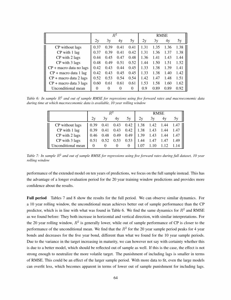
R2 RMSE2y 3y 4y 5y 2y 3y 4y 5y
CP without lags 0.37 0.39 0.41 0.41 1.31 1.35 1.36 1.38CP with 1 lag 0.37 0.39 0.41 0.42 1.31 1.36 1.37 1.38CP with 2 lags 0.44 0.45 0.47 0.48 1.36 1.41 1.43 1.44CP with 3 lags 0.48 0.49 0.51 0.52 1.44 1.50 1.51 1.52
CP + macro data no lags 0.42 0.43 0.44 0.45 1.33 1.38 1.39 1.41CP + macro data 1 lag 0.42 0.43 0.45 0.45 1.33 1.38 1.40 1.42CP + macro data 2 lags 0.52 0.53 0.54 0.54 1.42 1.47 1.48 1.51CP + macro data 3 lags 0.60 0.61 0.61 0.61 1.53 1.58 1.60 1.62
Unconditional mean 0 0 0 0 0.9 0.89 0.89 0.92
Table 6: In sample R2 and out of sample RMSE for regressions using five forward rates and macroeconomic dataduring time at which macroeconomic data is available, 10 year rolling window
R2 RMSE2y 3y 4y 5y 2y 3y 4y 5y
CP without lags 0.39 0.41 0.43 0.42 1.38 1.42 1.44 1.47CP with 1 lag 0.39 0.41 0.43 0.42 1.38 1.43 1.44 1.47CP with 2 lags 0.46 0.48 0.49 0.49 1.39 1.43 1.44 1.47CP with 3 lags 0.51 0.52 0.53 0.53 1.44 1.47 1.47 1.49
Unconditional mean 0 0 0 0 1.07 1.10 1.12 1.14
Table 7: In sample R2 and out of sample RMSE for regressions using five forward rates during full dataset, 10 yearrolling window
performance of the extended model on ten years of predictions, we focus on the full sample instead. This has
the advantage of a longer evaluation period for the 20 year training window predictions and provides more
confidence about the results.
Full period Tables 7 and 8 show the results for the full period. We can observe similar dynamics. For
a 10 year rolling window, the unconditional mean achieves better out of sample performance than the CP
predictor, which is in line with what was found in Table 6. We find the same dynamics for R2 and RMSE
as we found before: They both increase in horizontal and vertical direction, with similar interpretations. For
the 20 year rolling window, R2 is generally lower, while out of sample performance of CP is closer to the
performance of the unconditional mean. We find that the R2 for the 20 year sample period peaks for 4 year
bonds and decreases for the five year bond, different than what we found for the 10 year sample periods.
Due to the variance in the target increasing in maturity, we can however not say with certainty whether this
is due to a better model, which should be reflected out of sample as well. If this is the case, the effect is not
strong enough to neutralize the more volatile target. The punishment of including lags is smaller in terms
of RMSE. This could be an effect of the larger sample period. With more data to fit, even the large models
can overfit less, which becomes apparent in terms of lower out of sample punishment for including lags.
64

R2 RMSE2y 3y 4y 5y 2y 3y 4y 5y
CP without lags 0.30 0.31 0.32 0.30 0.85 0.87 0.88 0.90CP with 1 lag 0.30 0.31 0.32 0.30 0.85 0.87 0.87 0.89CP with 2 lags 0.36 0.37 0.38 0.36 0.85 0.87 0.88 0.89CP with 3 lags 0.39 0.39 0.41 0.39 0.84 0.87 0.88 0.90
Unconditional mean 0 0 0 0 0.76 0.78 0.82 0.83
Table 8: In sample R2 and out of sample RMSE for regressions using five forward rates during full dataset, 20 yearrolling window
The additional features do however not seem to help predict holding period excess returns: RMSE does not
decrease significantly when lags are included. Another finding that is consistent across sample periods is the
unconditional mean delivering out of sample predictions closer to actuals than the ones produced by the tent
proposed in Cochrane and Piazzesi (2005).
7.1.2 ANN prediction results
Period for which we have macroeconomic data Table 9, 10 and 11 depict the results for different ANNs
that we ran on the datasets available. We comment on performance for each of the three time periods indi-
vidually, and afterwards point out more general tendencies. As shown in Table 9, the overall performance in
terms of R2 is in between the performance of a simple CP regression and the regression including macroe-
conomic data with three lags (Table 6). The top performing ANN in sample is a linear restricted wide ANN.
Notably, it beats all of the benchmarks except the CP regression using macroeconomic data and three lags of
everything in terms of R2, while beating all benchmarks except the unconditional mean in terms of RMSE.
The model with the lowest RMSE is an unrestricted small model. It performs better than all benchmarks
except the unconditional mean out of sample and beats the simple CP model in terms of R2.
We find a general tendency for the ANNs that we also found for the benchmarks: Better in sample per-
formance is usually traded off against out of sample performance. In a horizontal direction, this is a natural
consequence of the target being more volatile. Across models it could be a sign of some models being more
flexible than others and fitting more noise. We analyse model flexibility further in the section on GDF in
order to make a definite judgement.
Overall, the ANNs perform slightly better than the regressions. They can achieve better in sample fit while
improving out of sample performance. It has to be noted, however, that the general level of RMSE is high.
Since these tests are performed on normalized data, the RMSE is about 50% higher than the standard
deviation of the training data, which can be assumed to be in the same general area as the standard deviation
of the test data. We thus still conclude that the ANNs do not predict excess returns well out of sample.
65
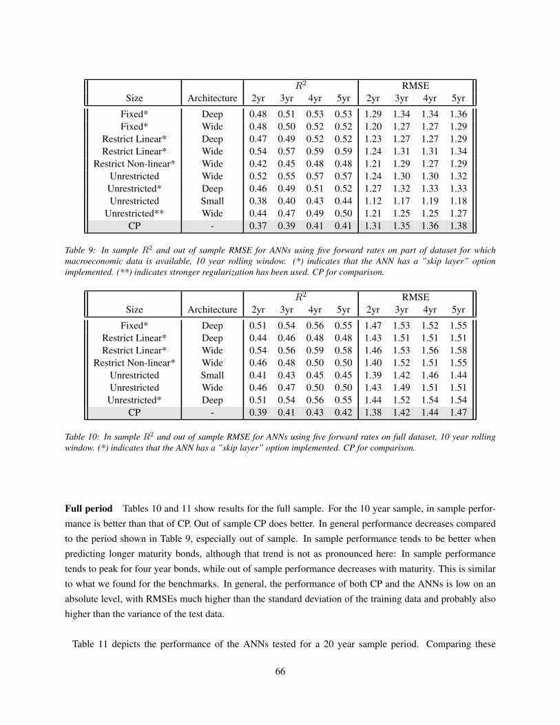
R2 RMSESize Architecture 2yr 3yr 4yr 5yr 2yr 3yr 4yr 5yr
Fixed* Deep 0.48 0.51 0.53 0.53 1.29 1.34 1.34 1.36Fixed* Wide 0.48 0.50 0.52 0.52 1.20 1.27 1.27 1.29
Restrict Linear* Deep 0.47 0.49 0.52 0.52 1.23 1.27 1.27 1.29Restrict Linear* Wide 0.54 0.57 0.59 0.59 1.24 1.31 1.31 1.34
Restrict Non-linear* Wide 0.42 0.45 0.48 0.48 1.21 1.29 1.27 1.29Unrestricted Wide 0.52 0.55 0.57 0.57 1.24 1.30 1.30 1.32Unrestricted* Deep 0.46 0.49 0.51 0.52 1.27 1.32 1.33 1.33Unrestricted Small 0.38 0.40 0.43 0.44 1.12 1.17 1.19 1.18
Unrestricted** Wide 0.44 0.47 0.49 0.50 1.21 1.25 1.25 1.27CP - 0.37 0.39 0.41 0.41 1.31 1.35 1.36 1.38
Table 9: In sample R2 and out of sample RMSE for ANNs using five forward rates on part of dataset for whichmacroeconomic data is available, 10 year rolling window. (*) indicates that the ANN has a ”skip layer” optionimplemented. (**) indicates stronger regularization has been used. CP for comparison.
R2 RMSESize Architecture 2yr 3yr 4yr 5yr 2yr 3yr 4yr 5yr
Fixed* Deep 0.51 0.54 0.56 0.55 1.47 1.53 1.52 1.55Restrict Linear* Deep 0.44 0.46 0.48 0.48 1.43 1.51 1.51 1.51Restrict Linear* Wide 0.54 0.56 0.59 0.58 1.46 1.53 1.56 1.58
Restrict Non-linear* Wide 0.46 0.48 0.50 0.50 1.40 1.52 1.51 1.55Unrestricted Small 0.41 0.43 0.45 0.45 1.39 1.42 1.46 1.44Unrestricted Wide 0.46 0.47 0.50 0.50 1.43 1.49 1.51 1.51Unrestricted* Deep 0.51 0.54 0.56 0.55 1.44 1.52 1.54 1.54
CP - 0.39 0.41 0.43 0.42 1.38 1.42 1.44 1.47
Table 10: In sample R2 and out of sample RMSE for ANNs using five forward rates on full dataset, 10 year rollingwindow. (*) indicates that the ANN has a ”skip layer” option implemented. CP for comparison.
Full period Tables 10 and 11 show results for the full sample. For the 10 year sample, in sample perfor-
mance is better than that of CP. Out of sample CP does better. In general performance decreases compared
to the period shown in Table 9, especially out of sample. In sample performance tends to be better when
predicting longer maturity bonds, although that trend is not as pronounced here: In sample performance
tends to peak for four year bonds, while out of sample performance decreases with maturity. This is similar
to what we found for the benchmarks. In general, the performance of both CP and the ANNs is low on an
absolute level, with RMSEs much higher than the standard deviation of the training data and probably also
higher than the variance of the test data.
Table 11 depicts the performance of the ANNs tested for a 20 year sample period. Comparing these
66

R2 RMSESize Architecture 2yr 3yr 4yr 5yr 2yr 3yr 4yr 5yr
Fixed* Wide 0.41 0.42 0.44 0.42 0.97 1.01 1.04 1.06Fixed* Deep 0.37 0.38 0.40 0.38 0.88 0.92 0.94 0.95
Restrict Linear* Wide 0.47 0.48 0.50 0.49 0.98 1.05 1.07 1.09Restrict Linear* Deep 0.38 0.39 0.41 0.40 0.92 0.98 1.00 1.02
Restrict Non-linear* Wide 0.32 0.32 0.34 0.33 0.84 0.89 0.90 0.93Unrestricted Wide 0.56 0.58 0.59 0.58 0.99 1.05 1.06 1.09
Unrestricted** Wide 0.32 0.32 0.34 0.33 0.83 0.87 0.90 0.93Unrestricted* Deep 0.38 0.39 0.42 0.40 0.90 0.96 0.97 0.98Unrestricted Small 0.33 0.33 0.36 0.35 0.83 0.87 0.90 0.93
Unrestricted** Wide 0.32 0.32 0.35 0.33 0.84 0.88 0.92 0.93CP - 0.30 0.31 0.32 0.30 0.85 0.87 0.88 0.90
Table 11: In sample R2 and out of sample RMSE for ANNs using five forward rates on full dataset, 20 year rollingwindow. (*) indicates that the ANN has a ”skip layer” option implemented. (**) indicates stronger regularization hasbeen used. CP for comparison.
results to those of the 10 year period, the relatively low in sample R2 is striking. There are some exceptions,
an unrestricted wide network does quite well in sample. That performance, however, is traded off against
out of sample performance: The unrestricted wide ANN is the worst out of sample predictor. Out of sample,
an unrestricted small ANN and a heavily regularized unrestricted wide network do best. Their better out of
sample performance, however, come at the expense of in sample goodness of fit, where the small network
manages to do slightly better than the heavily regularized wide one. Comparing to CP for the same period,
the ANNs manage to do better in sample. This is what one would expect, given that these models should be
more flexible. We measure model flexibility explicitly in the section on Generalized Degrees of Freedom.
Out-of-sample, the picture is more mixed, with the best ANNs doing better for shorter maturity bonds and
CP doing better for longer maturity bonds. The general level of performance out of sample is much better
than for the shorter sample periods. In general, both CP and the ANNs manage to get much closer to the out
of sample performance of the unconditional mean, which also gets a bit better.
In summary, the ANNs display better in sample fit, while they perform at about the same level as the
benchmark regressions out of sample. They display the same characteristics: Slightly worse out of sam-
ple performance for higher maturities, better in sample fit usually coming at the expense of out of sample
performance, and larger out of sample error than that of an unconditional mean forecast. Coming back to
our original question, whether we can find evidence of non linear combinations of forward rates predicting
excess returns, we cannot give a definite answer to that question based on the above results alone. The fact
that in sample fit increases for the period for which macroeconomic data is available, while out of sample
fit increases as well, seems encouraging. Comparing that result to the analysis of the full sample, however,
we do not find the same pattern. We get slightly higher in sample fit while paying for it with out of sample
67

performance. One possible interpretation is that the simple reason for better in sample performance is an in-
crease in degrees of freedom. Another explanation could be that there is a timing element to non-linearities
in the data. Feldhutter, Heyerdahl-Larsen, and Illeditsch (2013) state that non-linearities in the data vary over
time. If that is true, our models could display mixed results for an aggregate measure, while they at times do
better out of sample, while they overfit considerably at other times.
When we compare the 20 year period with the 10 year period, both the ANNs and regression predictors
do much better out of sample, while the CP predictors improve by much more than the ANNs. An explana-
tion could be the higher signal to noise ratio of what the models are fitting. Holding model size constant, this
naturally occurs when extending the training period. Measures like regularization or early stopping could
have mimicked this effect to a small degree when training the ANNs on 10 years of data. This phenomenon
would make a 20 year sample period a more meaningful base for comparison.
In light of the above results, it is interesting whether the ANNs predictions are similar to the ones made
by CP. If the ANNs achieve the same predictive performance out of sample while making very different
predictions, they might discover something in the data that is not captured by CP, while not capturing the
same signal as CP. If the models that allow for non-linearities recover the same factor as the CP regressions,
that would on the other hand strengthen the claim of five factors predicting excess returns made in Cochrane
and Piazzesi (2005).
7.2 Absolute performance
The result that the mean achieves the lowest RMSE of all the predictors raises the question whether it is even
relevant to consider relative performance. In this section we consider possible implications of this absolute
performance and we argue that while the fact that the mean wins out of sample is certainly interesting, the
way it wins makes it less interesting in the discussion of the EH and the predictive factor that Cochrane and
Piazzesi (2005) identify.
First, we relate the out of sample performance directly to the original finding. We follow on findings of
unspanned factors (e.g. Ludvigson and Ng (2009)) by comparing the headline figure of these paper, the in
sample R2IS to the out of sample R2
OS from the predictions based on corresponding samples. We acknowl-
edge that Cochrane and Piazzesi (2005) calculate a host of additional statistics to investigate the results they
find, but the difference between in and out of sample performance is very clearly reflected in this measure.
68
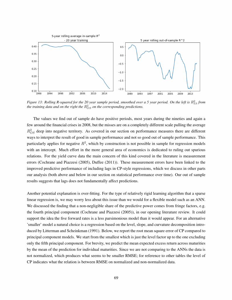
Figure 13: Rolling R-squared for the 20 year sample period, smoothed over a 5 year period. On the left is R2IS from
the training data and on the right the R2OS on the corresponding predictions.
The values we find out of sample do have positive periods, most years during the nineties and again a
few around the financial crises in 2008, but the misses are on a completely different scale pulling the average
R2OS deep into negative territory. As covered in our section on performance measures there are different
ways to interpret the result of good in sample performance and not so good out of sample performance. This
particularly applies for negative R2, which by construction is not possible in sample for regression models
with an intercept. Much effort in the more general area of economics is dedicated to ruling out spurious
relations. For the yield curve data the main concern of this kind covered in the literature is measurement
errors (Cochrane and Piazzesi (2005), Duffee (2011)). These measurement errors have been linked to the
improved predictive performance of including lags in CP-style regressions, which we discuss in other parts
our analysis (both above and below in our section on statistical performance over time). Our out of sample
results suggests that lags does not fundamentally affect predictions.
Another potential explanation is over-fitting. For the type of relatively rigid learning algorithm that a sparse
linear regression is, we may worry less about this issue than we would for a flexible model such as an ANN.
We discussed the finding that a non-negligible share of the predictive power comes from fringe factors, e.g.
the fourth principal component (Cochrane and Piazzesi (2005)), in our opening literature review. It could
support the idea the five forward rates is a less parsimonious model than it would appear. For an alternative
’smaller’ model a natural choice is a regression based on the level, slope, and curvature decomposition intro-
duced by Litterman and Scheinkman (1991). Below, we report the root mean square error of CP compared to
principal component models. We start from the smallest which is just the level factor up to the one excluding
only the fifth principal component. For brevity, we predict the mean expected excess return across maturities
by the mean of the prediction for individual maturities. Since we are not comparing to the ANNs the data is
not normalized, which produces what seems to be smaller RMSE; for reference to other tables the level of
CP indicates what the relation is between RMSE on normalized and non-normalized data.
69
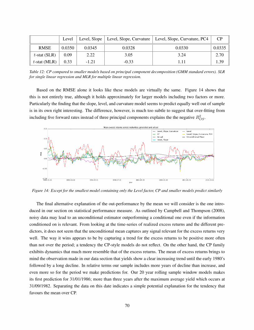
Level Level, Slope Level, Slope, Curvature Level, Slope, Curvature, PC4 CP
RMSE 0.0350 0.0345 0.0328 0.0330 0.0335
t-stat (SLR) 0.09 2.22 3.05 3.24 2.70
t-stat (MLR) 0.33 -1.21 -0.33 1.11 1.39
Table 12: CP compared to smaller models based on principal component decomposition (GMM standard errors). SLRfor single linear regression and MLR for multiple linear regression.
Based on the RMSE alone it looks like these models are virtually the same. Figure 14 shows that
this is not entirely true, although it holds approximately for larger models including two factors or more.
Particularly the finding that the slope, level, and curvature model seems to predict equally well out of sample
is in its own right interesting. The difference, however, is much too subtle to suggest that over-fitting from
including five forward rates instead of three principal components explains the the negative R2OS .
Figure 14: Except for the smallest model containing only the Level factor, CP and smaller models predict similarly
The final alternative explanation of the out-performance by the mean we will consider is the one intro-
duced in our section on statistical performance measure. As outlined by Campbell and Thompson (2008),
noisy data may lead to an unconditional estimator outperforming a conditional one even if the information
conditioned on is relevant. From looking at the time-series of realized excess returns and the different pre-
dictors, it does not seem that the unconditional mean captures any signal relevant for the excess returns very
well. The way it wins appears to be by capturing a trend for the excess returns to be positive more often
than not over the period; a tendency the CP-style models do not reflect. On the other hand, the CP family
exhibits dynamics that much more resemble that of the excess returns. The mean of excess returns brings to
mind the observation made in our data section that yields show a clear increasing trend until the early 1980’s
followed by a long decline. In relative terms our sample includes more years of decline than increase, and
even more so for the period we make predictions for. Our 20 year rolling sample window models makes
its first prediction for 31/01/1986; more than three years after the maximum average yield which occurs at
31/09/1982. Separating the data on this date indicates a simple potential explanation for the tendency that
favours the mean over CP.
70

Average realized excess returns 2 yr→ 1 yr 3 yr→ 2 yr 4 yr→ 3 yr 5 yr→ 4 yr
1965-01 to 1982-09 -0.005 -0.009 -0.014 -0.019
1982-09 to 2015-12 0.010 0.019 0.026 0.031
Average CP prediction 2 yr→ 1 yr 3 yr→ 2 yr 4 yr→ 3 yr 5 yr→ 4 yr
1976-01 to 1982-09 0.0125 0.0169 0.0205 0.0244
1982-09 to 2015-12 -0.0025 -0.0067 -0.0097 -0.0146
Table 13: Averages of realized excess returns and predictions from the CP regressions estimated on a 10 year rollingwindow. 1982-09 is the month with the maximum average yield, after this month yields have declined.
Not only does increasing (decreasing) yields seem to produce negative (positive) average realized excess
returns, the effect on CP is inverted, leading to positive prediction (on average) in the former period and
negative in the latter. What the mean gets right, may simply be getting the level less wrong.
Capturing dynamics To get an estimate of the significance of the relations we quantify correlations by
regressions. The standard errors of these regressions are based on rolling estimates and are as such serially
correlated. Furthermore the two step procedure of estimating the regressors could cause heteroskedasticity by
”bold” misses on average overshooting the target by a larger margin. To make this clear, it is key to remember
that the explanatory variable in the regression here is the prediction from the model under consideration.
Heteroskedasticity in this case would be a correlation between model predictions and the residual of fitting
the realized returns to these predictions. Overall we find reason to be cautious and apply the very general
correction of standard errors from the GMM framework that we also used to reproduce the Cochrane and
Piazzesi (2005) results.
71
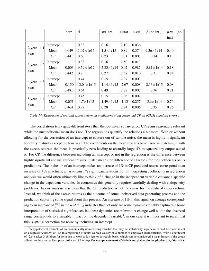
corr β std. err. t-stat p-val β (no int.) p-val (no
int.)
2 year→ 1
year
Intercept 0.33 0.16 2.10 0.036
Mean 0.049 1.02×1e15 1.5×1e15 0.89 0.374 9.36×1e14 0.40
CP 0.441 0.66 0.23 2.81 0.005 0.34 0.13
3 year→ 2
year
Intercept 0.38 0.16 2.50 0.013
Mean -0.003 9.59×1e12 5.83×1e14 0.02 0.987 -5.81×1e14 0.18
CP 0.442 0.7 0.27 2.57 0.010 0.31 0.24
4 year→ 3
year
Intercept 0.44 0.15 2.97 0.003
Mean -0.150 -3.04×1e15 1.14×1e15 -2.67 0.008 -2.13×1e15 0.08
CP 0.481 0.64 0.49 2.82 0.005 0.36 0.21
5 year→ 4
year
Intercept 0.45 0.15 3.06 0.002
Mean -0.051 -1.7×1e15 1.49×1e15 -1.13 0.257 -5.6×1e14 0.76
CP 0.464 0.77 0.28 2.74 0.006 0.35 0.26
Table 14: Regression of realized excess return on predictions of the mean and CP on (GMM standard errors).
The correlations tell a quite different story than the root mean square error: CP seems reasonably relevant
while the unconditional mean does not. The regressions quantify the relations a bit more. With or without
allowing for the correction of an intercept to capture out of sample noise, the mean is highly insignificant
for every maturity except the four year. The coefficients on the mean reveal a basic issue in matching it with
the excess returns: the mean is practically zero leading to absurdly large β’s to squeeze any output out of
it. For CP, the difference between including an intercept or not in the regression is the difference between
highly significant and insignificant results. It also means the difference of a factor 2 for the coefficients on its
predictions. The inclusion of an intercept makes an increase of 1% in CP predicted returns correspond to an
increase of 23% in actuals; an economically significant relationship. In interpreting coefficients in regression
analysis we would often ultimately like to think of a change in the independent variable causing a specific
change in the dependent variable. In economics this generally requires carefully dealing with endogeneity
problems. In our analysis it is clear that the CP prediction is not the cause for the realized excess return.
Instead, we think of the excess returns as the outcome of some unobserved data generating process and the
prediction capturing some signal about this process. An increase of 1% in this signal on average correspond-
ing to an increase of 23% in the real thing indicates that not only are some dynamics reliably captured (a loose
interpretation of statistical significance), but these dynamics are relevant. A change well within the observed
range corresponds to a sizeable impact on the dependent variable9; in our case it is important to recall that
this is after a correction for noise by including an intercept.9A hypothetical example of an economically uninteresting variable that may be statistically significant would be a coefficient
on a regressor children of -2.6 in a regression of hours worked weekly on a number of employee characteristics. With a coefficientof -2.6 it takes 3 children for someone to work a day less on a weekly basis, which can be considered a weak impact if the groupadheres to the average European birth rate of 1.6 http://ec.europa.eu/eurostat/statistics-explained/index.php/Fertility˙statistics
72
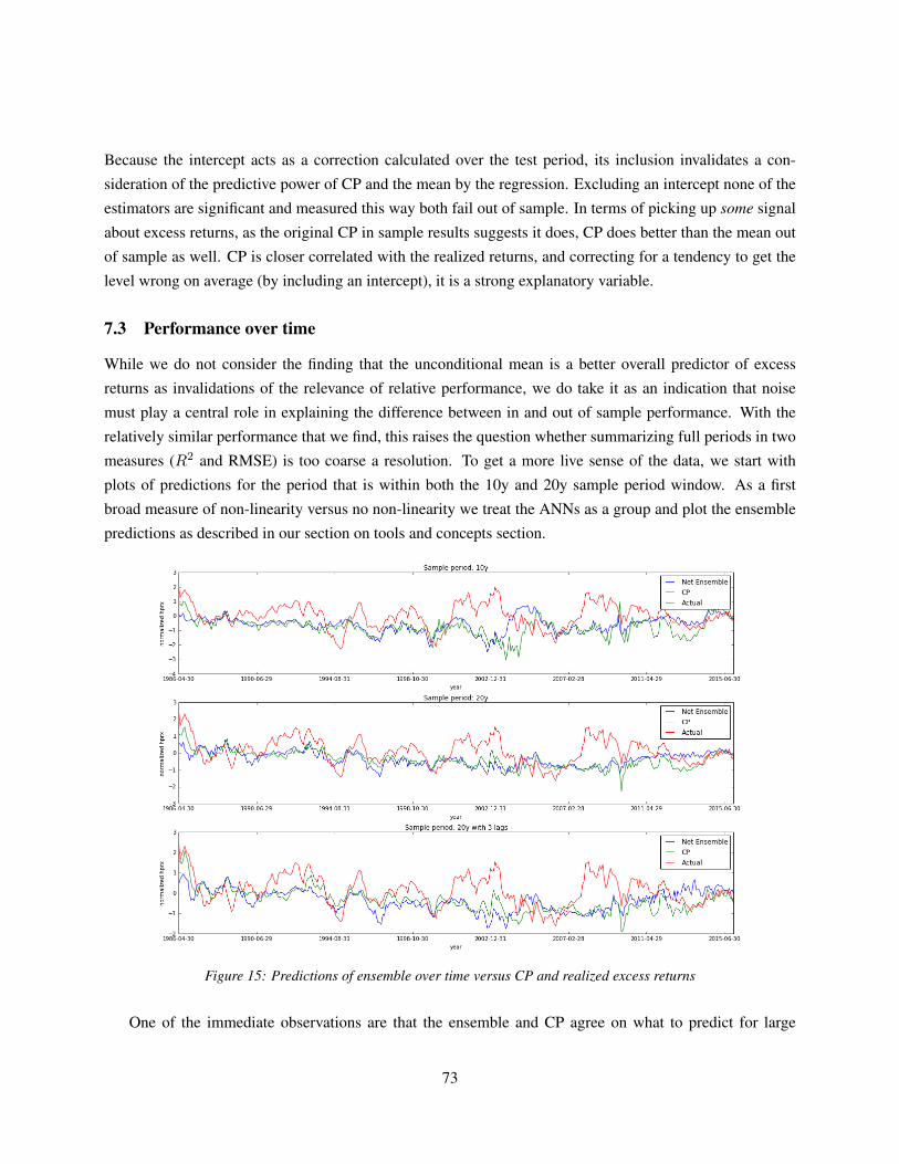
Because the intercept acts as a correction calculated over the test period, its inclusion invalidates a con-
sideration of the predictive power of CP and the mean by the regression. Excluding an intercept none of the
estimators are significant and measured this way both fail out of sample. In terms of picking up some signal
about excess returns, as the original CP in sample results suggests it does, CP does better than the mean out
of sample as well. CP is closer correlated with the realized returns, and correcting for a tendency to get the
level wrong on average (by including an intercept), it is a strong explanatory variable.
7.3 Performance over time
While we do not consider the finding that the unconditional mean is a better overall predictor of excess
returns as invalidations of the relevance of relative performance, we do take it as an indication that noise
must play a central role in explaining the difference between in and out of sample performance. With the
relatively similar performance that we find, this raises the question whether summarizing full periods in two
measures (R2 and RMSE) is too coarse a resolution. To get a more live sense of the data, we start with
plots of predictions for the period that is within both the 10y and 20y sample period window. As a first
broad measure of non-linearity versus no non-linearity we treat the ANNs as a group and plot the ensemble
predictions as described in our section on tools and concepts section.
Figure 15: Predictions of ensemble over time versus CP and realized excess returns
One of the immediate observations are that the ensemble and CP agree on what to predict for large
73

periods of time regardless of the sampling window. This is reflected in correlation which is markedly higher
between the two time-series than the correlation with realized returns.
10y 20y 20y with 3 lags
Correlation between Ensemble and CP 0.49 0.68 0.66
Correlation with realized returns Ensemble 0.01 0.21 0.19
Correlation with realized returns CP 0.15 0.43 0.44
RMSE Ensemble 0.9 0.73 0.77
RMSE CP 1.0 0.68 0.67
Table 15: Correlation and RMSE in predictions 1986-04 to 2015-06
The correlation between the ensemble predictions and the realized returns for the 10y sample period
look particularly low, especially taking into account that the RMSE for the 10y sample window ensemble
predictions are 0.9 while CP is 1.0; a 10% improvement from worse to better in favour of the ANNs. Just
as reported in our section on overall results, the RMSE for the longer estimation window is better for both
CP and the ANNs, but now CP comes out ahead with an RMSE of 0.68 versus 0.73 (6.8% improvement).
Including lags does not really affect CP performance, but ensemble performance deteriorates slightly on both
RMSE and correlations with realized returns. From the plots it does, however, it seems wrong to say that the
CP predictions are unaffected by the inclusion of lags. In the very beginning of the period, early 1994 and
in the end of 2002 are all examples of periods when lags seem to help CP get closer to actual returns. One
possibility is that lags simply increase volatility, and misses are equally amplified. In aggregated numbers,
the volatility for the rolling 20y period increases by 35% for CP and 20% for the ANNs when lags are
included as explanatory variables. For CP, the average over the period is stable across the two specifications
corroborating the view that predictions are simply amplified.
10y 20y 20y with 3 lags
Realized returns volatility 0.83 0.75 0.75
CP volatility 0.64 0.49 0.66
Ensemble volatility 0.54 0.44 0.53
Realized returns average -0.01 0.11 0.11
CP average -0.78 -0.38 -0.37
Ensemble average -0.6 -0.36 -0.38
Table 16: Average and volatility of predictions 1986-04 to 2015-06. The different normalization horizon explains thedifferences in the statistics for the realized returns.
For the ensemble the story is similar, but with a performance loss of 5% on RMSE and 10% on the
correlation, the amplification is not entirely neutral. While the magnitude of this non-neutrality seems small
74

taking into account the overall noisiness of the data, and the randomness involved in the training of the ANNs,
the ensemble approach assures a certain level of averaging out which limits the scope for these two driving
results. From the plots three periods stand out: around beginning of 1994 where CP improves by spiking
more, the ensemble predictions becomes smoother. In the end of 2002 where predictions are amplified, but
the trend predicted is more negative; and finally, the last 3-4 years of data where increased volatility seems
to hurt the ensemble as it is already misses a dip in excess returns that it captures when trained on a 10y
window.
A closer look at the impact of sample window Table 16 and 15 demonstrates the large impact of the
size of the training sample. The normalization alone are responsible for a 10% increase in volatility for
the realized returns, but even on a realized returns volatility weighted basis CP and the ensemble are more
volatile when estimated on the short period: 0.77 vs 0.65 for CP, and 0.65 vs 0.58 for the ANNs. For the
average realized returns the percentage differences becomes very large because the 10y average is so close
to zero. As the data is normalised, zero would be the average of the realized returns if the training data and
the testing data on average had the same mean. The volatility would be 1 if the training data and the testing
data on average had the same variance. For periods of 11 years (10 years of training + 1 for testing on the
return a year later) the excess return has on average been similar whereas for 21 years the realised excess
return has on average been higher at the end of the period than throughout the period. For both sample
windows the volatility has on average been lower at the end. Both CP and the ensemble are more successful
in matching the volatility than finding the mean, but the discrepancy between training and testing mean is
less important than having more training cases; the gap between the average of predictions and actual excess
returns are -0.77 versus -0.49 for CP, and -0.59 versus -0.47 for the ANNs. While decreasing the distance
to the mean, the two different approaches are also converging to a common prediction. A 39% increase in
correlation between the two sets of predictions indicates that this convergence is broader than the prediction
of the average. Putting the pieces together we conjecture that the signal we find with either approach is the
same, and that the relation behind the signal is stable enough to make filtering out noise more important
than reacting to potential shifts in the underlying process. In the bigger picture, non-linearity does not seem
to improve the processing of this signal; the flexibility required to allow for it may actually obscure the it.
In sections below we explicitly cover the cross-section, considering both the flexibility provided by larger
degrees of freedom, and the allowance for non-linearity.
7.4 Results of economic tests
7.4.1 Benchmark performance
Period for which we have macroeconomic data As for the statistical measures, we use the CP regressions
in different combinations with lags and macroeconomic indicators as benchmarks for our models. We report
annualized returns, annualized volatility, and SR, which is the former divided by the latter. We first consider
the time period for which macroeconomic data is available to us (Table 17). During that time period none of
75
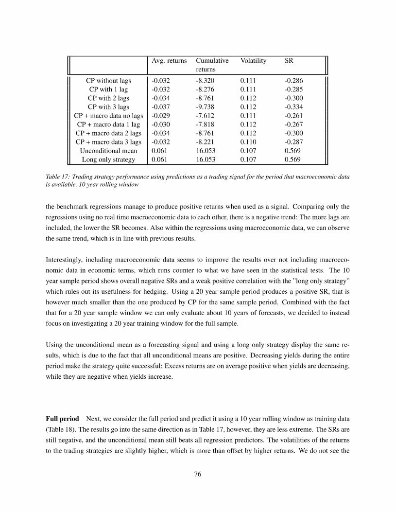
Avg. returns Cumulativereturns
Volatility SR
CP without lags -0.032 -8.320 0.111 -0.286CP with 1 lag -0.032 -8.276 0.111 -0.285CP with 2 lags -0.034 -8.761 0.112 -0.300CP with 3 lags -0.037 -9.738 0.112 -0.334
CP + macro data no lags -0.029 -7.612 0.111 -0.261CP + macro data 1 lag -0.030 -7.818 0.112 -0.267CP + macro data 2 lags -0.034 -8.761 0.112 -0.300CP + macro data 3 lags -0.032 -8.221 0.110 -0.287
Unconditional mean 0.061 16.053 0.107 0.569Long only strategy 0.061 16.053 0.107 0.569
Table 17: Trading strategy performance using predictions as a trading signal for the period that macroeconomic datais available, 10 year rolling window
the benchmark regressions manage to produce positive returns when used as a signal. Comparing only the
regressions using no real time macroeconomic data to each other, there is a negative trend: The more lags are
included, the lower the SR becomes. Also within the regressions using macroeconomic data, we can observe
the same trend, which is in line with previous results.
Interestingly, including macroeconomic data seems to improve the results over not including macroeco-
nomic data in economic terms, which runs counter to what we have seen in the statistical tests. The 10
year sample period shows overall negative SRs and a weak positive correlation with the ”long only strategy”
which rules out its usefulness for hedging. Using a 20 year sample period produces a positive SR, that is
however much smaller than the one produced by CP for the same sample period. Combined with the fact
that for a 20 year sample window we can only evaluate about 10 years of forecasts, we decided to instead
focus on investigating a 20 year training window for the full sample.
Using the unconditional mean as a forecasting signal and using a long only strategy display the same re-
sults, which is due to the fact that all unconditional means are positive. Decreasing yields during the entire
period make the strategy quite successful: Excess returns are on average positive when yields are decreasing,
while they are negative when yields increase.
Full period Next, we consider the full period and predict it using a 10 year rolling window as training data
(Table 18). The results go into the same direction as in Table 17, however, they are less extreme. The SRs are
still negative, and the unconditional mean still beats all regression predictors. The volatilities of the returns
to the trading strategies are slightly higher, which is more than offset by higher returns. We do not see the
76

Avg. returns Cumulative returns Volatility SR
CP without lags -0.020 -9.810 0.156 -0.131CP with 1 lag -0.021 -9.869 0.156 -0.132CP with 2 lags -0.025 -12.084 0.150 -0.169CP with 3 lags -0.017 -7.974 0.152 -0.110
Unconditional mean 0.034 16.116 0.150 0.223Long only strategy 0.058 27.451 0.153 0.375
Table 18: Trading strategy performance using predictions as a trading signal for the full period, 10 year rolling window
Avg. returns Cumulative returns Volatility SR
CP without lags 0.030 10.976 0.132 0.231CP with 1 lag 0.030 10.698 0.132 0.226CP with 2 lags 0.027 9.715 0.131 0.207CP with 3 lags 0.023 8.124 0.131 0.174
Unconditional mean 0.053 19.080 0.130 0.409Long only strategy 0.076 27.168 0.118 0.642
Table 19: Trading strategy performance using predictions as a trading signal for the full period, 20 year rolling window
same tendency as in Table 17: As we include more lags, the annualized returns first decrease, just to increase
for 3 lags. Overall negative SRs and weak positive correlation with the long only strategy make the 10 year
window less interesting to consider: The weak correlation rules it out as a valuable hedge to the long-only
strategy.
We consider 20 year rolling training periods next. The results of the strategies are depicted in Table
19. The CP predictors deliver a much better economic performance than for the 10 year period, as do the
unconditional mean and the long only strategy. Good results of the long only strategy have to be taken with
caution, as they could be due to decreasing yields in that time period. Volatility is lower and the return higher.
Analogue to the statistical performance, this could be a consequence of a higher signal to noise ratio with
a longer sample period. Additionally, the same trend as in Table 17 emerges and more lags result in worse
performance. In summary, the signal from performing CP regressions on a 20 year sample period seems to
be more economically meaningful than the other signals considered beforehand: Its positive returns make it
lucrative. Weak positive correlation of the 10 year sample period strategy with the long only strategy make
that one unsuitable for hedging, thus leaving the 20 year sample period the most interesting.
7.4.2 ANN predictions
Period for which we have macroeconomic data In Table 20, the results are depicted. Comparing them
to those of the benchmarks (Table 17) during that period, the ANNs do much better. The top performer
is the wide unrestricted ANN with a wide unrestricted ANN with heavy regularization following closely.
77

Architecture Size Avg. returns Cumulative returns Volatility SR
Fixed* Wide -0.014 -3.780 0.115 -0.125Fixed* Deep -0.022 -5.677 0.113 -0.190
Restrict Linear* Deep -0.013 -3.430 0.116 -0.112Restrict Linear* Wide -0.010 -2.563 0.115 -0.084
Restrict Non-linear* Wide -0.016 -4.090 0.112 -0.139Unrestricted Wide -0.004 -1.039 0.117 -0.034Unrestricted Small -0.008 -2.207 0.114 -0.074
Unrestricted** Wide -0.006 -1.474 0.119 -0.047Unrestricted* Deep -0.009 -2.468 0.114 -0.082
CP - -0.032 -8.320 0.111 -0.286
Table 20: Trading strategy performance using ANN predictions as a trading signal for the period that macroeconomicdata is available, 10 year rolling. (*) indicates that the ANN has a ”skip layer” option implemented. (**) indicatesstronger regularization has been used. CP for comparison
Architecture Size Avg. returns Cumulative returns Volatility SR
Fixed* Deep -0.020 -9.650 0.154 -0.131Restrict Linear* Wide -0.014 -6.489 0.155 -0.087Restrict Linear* Deep -0.022 -10.546 0.151 -0.145
Restrict Non-linear* Wide -0.013 -6.431 0.146 -0.092Unrestricted Wide -0.008 -3.975 0.158 -0.052Unrestricted Small -0.006 -2.798 0.148 -0.040
Unrestricted* Deep -0.013 -6.066 0.152 -0.083CP - -0.020 -9.810 0.156 -0.131
Table 21: Trading strategy performance using ANN predictions as a trading signal for the full period, 10 year rolling(*) indicates that the ANN has a ”skip layer” option implemented.
Interestingly, the trading strategies using ANN predictions have roughly the same volatility as the strategies
depicted in Table 17 and win by delivering superior (less negative) returns. The absolute performance is still
poor, with all the predictors being outperformed by a simple historical mean.
Full period In Table 21 we show the returns of a trading strategy using ANNs trained on a 10 year rolling
window of training data for the full sample period. The returns for all strategies are negative, while being
considerably higher than the ones for CP. The winner is a small unrestricted ANN, as in the section on sta-
tistical performance. The small unrestricted ANN delivers about the same returns as the wide unrestricted
ANN with heavy regularization in Table 20. The direct restriction on their size and the regularization restrict-
ing the size of the weights appear to work in the same direction. The strategy returns have higher volatility
than the same strategies during the period for which we have macroeconomic data. In absolute terms, the
performance is considerably worse than using the unconditional mean as a signal or a long only strategy.
Lastly, we run the same analysis using a 20 year rolling training window. The results are much better in
78
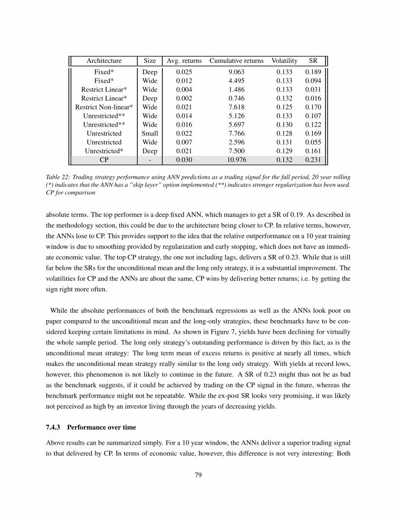
Architecture Size Avg. returns Cumulative returns Volatility SR
Fixed* Deep 0.025 9.063 0.133 0.189Fixed* Wide 0.012 4.495 0.133 0.094
Restrict Linear* Wide 0.004 1.486 0.133 0.031Restrict Linear* Deep 0.002 0.746 0.132 0.016
Restrict Non-linear* Wide 0.021 7.618 0.125 0.170Unrestricted** Wide 0.014 5.126 0.133 0.107Unrestricted** Wide 0.016 5.697 0.130 0.122
Unrestricted Small 0.022 7.766 0.128 0.169Unrestricted Wide 0.007 2.596 0.131 0.055Unrestricted* Deep 0.021 7.500 0.129 0.161
CP - 0.030 10.976 0.132 0.231
Table 22: Trading strategy performance using ANN predictions as a trading signal for the full period, 20 year rolling(*) indicates that the ANN has a ”skip layer” option implemented.(**) indicates stronger regularization has been used.CP for comparison
absolute terms. The top performer is a deep fixed ANN, which manages to get a SR of 0.19. As described in
the methodology section, this could be due to the architecture being closer to CP. In relative terms, however,
the ANNs lose to CP. This provides support to the idea that the relative outperformance on a 10 year training
window is due to smoothing provided by regularization and early stopping, which does not have an immedi-
ate economic value. The top CP strategy, the one not including lags, delivers a SR of 0.23. While that is still
far below the SRs for the unconditional mean and the long only strategy, it is a substantial improvement. The
volatilities for CP and the ANNs are about the same, CP wins by delivering better returns; i.e. by getting the
sign right more often.
While the absolute performances of both the benchmark regressions as well as the ANNs look poor on
paper compared to the unconditional mean and the long-only strategies, these benchmarks have to be con-
sidered keeping certain limitations in mind. As shown in Figure 7, yields have been declining for virtually
the whole sample period. The long only strategy’s outstanding performance is driven by this fact, as is the
unconditional mean strategy: The long term mean of excess returns is positive at nearly all times, which
makes the unconditional mean strategy really similar to the long only strategy. With yields at record lows,
however, this phenomenon is not likely to continue in the future. A SR of 0.23 might thus not be as bad
as the benchmark suggests, if it could be achieved by trading on the CP signal in the future, whereas the
benchmark performance might not be repeatable. While the ex-post SR looks very promising, it was likely
not perceived as high by an investor living through the years of decreasing yields.
7.4.3 Performance over time
Above results can be summarized simply. For a 10 year window, the ANNs deliver a superior trading signal
to that delivered by CP. In terms of economic value, however, this difference is not very interesting: Both
79
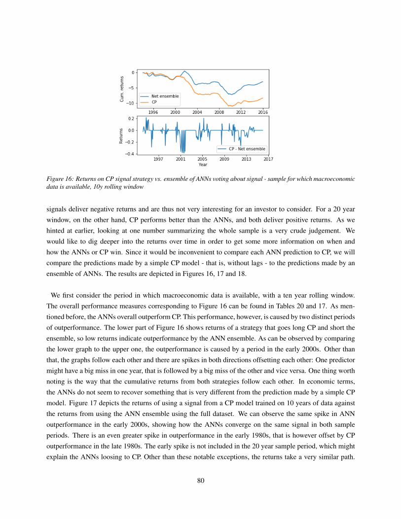
Figure 16: Returns on CP signal strategy vs. ensemble of ANNs voting about signal - sample for which macroeconomicdata is available, 10y rolling window
signals deliver negative returns and are thus not very interesting for an investor to consider. For a 20 year
window, on the other hand, CP performs better than the ANNs, and both deliver positive returns. As we
hinted at earlier, looking at one number summarizing the whole sample is a very crude judgement. We
would like to dig deeper into the returns over time in order to get some more information on when and
how the ANNs or CP win. Since it would be inconvenient to compare each ANN prediction to CP, we will
compare the predictions made by a simple CP model - that is, without lags - to the predictions made by an
ensemble of ANNs. The results are depicted in Figures 16, 17 and 18.
We first consider the period in which macroeconomic data is available, with a ten year rolling window.
The overall performance measures corresponding to Figure 16 can be found in Tables 20 and 17. As men-
tioned before, the ANNs overall outperform CP. This performance, however, is caused by two distinct periods
of outperformance. The lower part of Figure 16 shows returns of a strategy that goes long CP and short the
ensemble, so low returns indicate outperformance by the ANN ensemble. As can be observed by comparing
the lower graph to the upper one, the outperformance is caused by a period in the early 2000s. Other than
that, the graphs follow each other and there are spikes in both directions offsetting each other: One predictor
might have a big miss in one year, that is followed by a big miss of the other and vice versa. One thing worth
noting is the way that the cumulative returns from both strategies follow each other. In economic terms,
the ANNs do not seem to recover something that is very different from the prediction made by a simple CP
model. Figure 17 depicts the returns of using a signal from a CP model trained on 10 years of data against
the returns from using the ANN ensemble using the full dataset. We can observe the same spike in ANN
outperformance in the early 2000s, showing how the ANNs converge on the same signal in both sample
periods. There is an even greater spike in outperformance in the early 1980s, that is however offset by CP
outperformance in the late 1980s. The early spike is not included in the 20 year sample period, which might
explain the ANNs loosing to CP. Other than these notable exceptions, the returns take a very similar path.
80
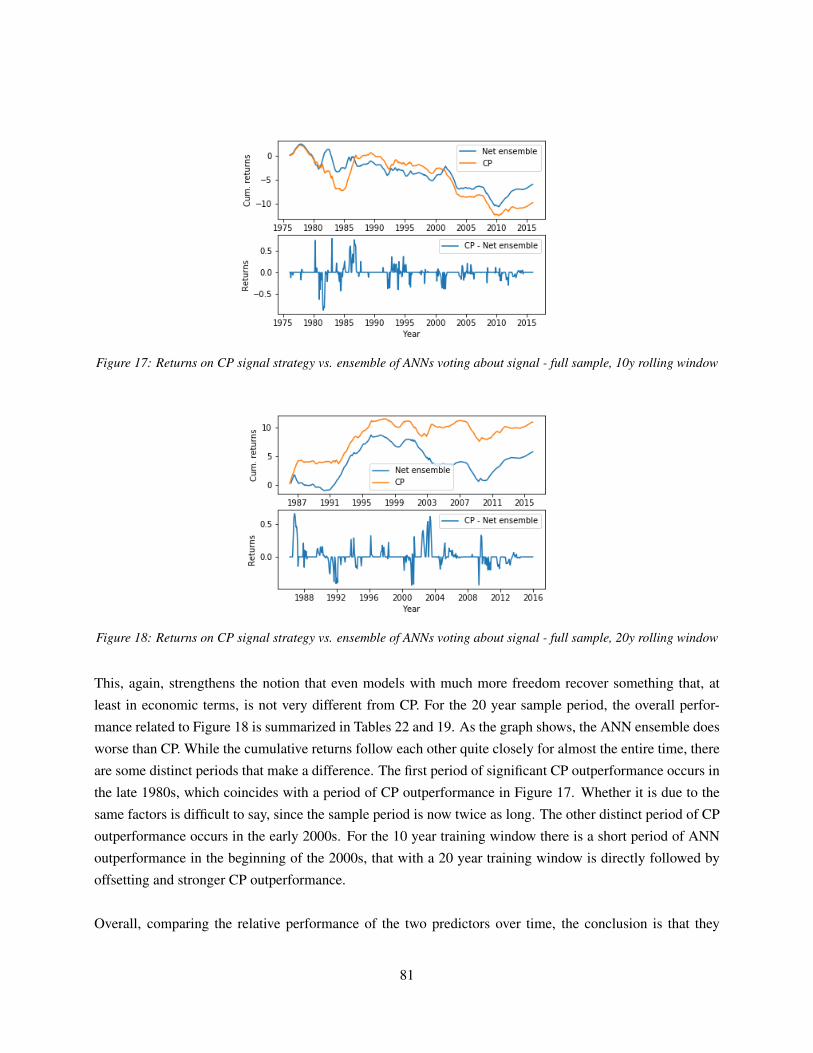
Figure 17: Returns on CP signal strategy vs. ensemble of ANNs voting about signal - full sample, 10y rolling window
Figure 18: Returns on CP signal strategy vs. ensemble of ANNs voting about signal - full sample, 20y rolling window
This, again, strengthens the notion that even models with much more freedom recover something that, at
least in economic terms, is not very different from CP. For the 20 year sample period, the overall perfor-
mance related to Figure 18 is summarized in Tables 22 and 19. As the graph shows, the ANN ensemble does
worse than CP. While the cumulative returns follow each other quite closely for almost the entire time, there
are some distinct periods that make a difference. The first period of significant CP outperformance occurs in
the late 1980s, which coincides with a period of CP outperformance in Figure 17. Whether it is due to the
same factors is difficult to say, since the sample period is now twice as long. The other distinct period of CP
outperformance occurs in the early 2000s. For the 10 year training window there is a short period of ANN
outperformance in the beginning of the 2000s, that with a 20 year training window is directly followed by
offsetting and stronger CP outperformance.
Overall, comparing the relative performance of the two predictors over time, the conclusion is that they
81

are not very different. Some distinct periods dictate which one of the strategies win, but their similarity is
hidden in the aggregate measures and is only discovered in an analysis of performance over time. We note
that the ANNs make predictions similar to those of CP for many of the periods. There are even many periods
where the trading signals do not differ at all, as indicated by longer stretches without spikes in Figures 17,
16 and 18.
7.5 (Generalized) degrees of freedom
In addition to comparing the predictions of the models we are using, we would like to investigate other fea-
tures of the models we use. As pointed out in the tools and concepts section, ANNs can in theory fit any
training data if they are complex enough (Winkler and Le (2017)). While testing the models out of sample
provides a natural safeguard against overfitting, we will provide an additional measure of model complexity.
As pointed out among others in Ye (1998), who mentions the AIC and the BIC, the degrees of freedom of
linear models are often used as a measure of model complexity. Especially when conducting only in sam-
ple studies, controlling for model complexity is very important. In our tools and concepts section, we have
provided an example of why controlling for model complexity matters: Figure 4 illustrates that a powerful
model such as an ANN could be fitting noise instead of the true signal in the data.
As explained in the section on GDF, calculating the degrees of freedom for simple regression models is
quite straightforward: The number of features equal the degrees of freedom. As shown in that section, the
GDF algorithm should theoretically simplify to the degrees of freedom. The results are shown in Table 23.
The CP estimation was done as a sanity check. As becomes apparent from the number for CP, the estimate
is not completely accurate.
82

Architecture Size GDF estimate
CP - 7.2
CP (3 lags) - 22.39
Fixed* Wide 9.62 - 45.9
Fixed* Deep 7.89 - 28.82
Restrict linear* Wide 12.15 - 43.77
Restrict linear* Deep 8.85 - 34.91
Restrict non linear* Wide 9.14 - 38.25
Unrestricted* Deep 9.3 - 32.69
Unrestricted Wide 8.02 - 18.06
Unrestricted Small 8.24 - 21.52
Unrestricted Deep 10.14 - 39.97
Table 23: Estimated GDF for different models, including CP as a benchmark. (*) indicates that the ANN has a ”skiplayer” option implemented.
Although they are clearly approximations, the numbers should still give a good indication of model flex-
ibility, since they are ultimately a numerical sensitivity of the model to small changes in the target. The
estimates for the ANNs are reported as ranges. The reason for that is training time has an effect on model
flexibility. In some initial analyses we found that the optimal number of epochs 10, was fairly low. When
we estimate the GDF using these few iterations, we get a GDF estimate at the lower end of these ranges.
This can be interpreted as the effective model flexibility for the models we used to make our predictions.
On the other hand, it is interesting to also know how flexible these models are when they are trained to the
limit. We used 1000 epochs 11 and found much higher model flexibility. This number is reported as the
high end of the range and can be interpreted as the flexibility of the model itself, as opposed to the flex-
ibility of the models as implemented by us. The clear takeaway is that the ANNs are less complicated as
one might expect when measures to avoid overfitting such as early stopping and regularization are employed.
Connecting statistical performance with the GDF estimates, we find that ANNs that perform good in sample
are on the upper end of GDF scale. Our top in sample performer, the wide ANN with a linear restriction, has
the highest effective (lower end) GDF. The ANN with the second highest effective GDF estimate, the unre-
stricted deep ANN, does best in sample for the 20 year period (Table 22). For out of sample performance,
we find an opposite tendency. The ANN with the best out of sample performance, the small unrestricted
ANN, has one of the lowest GDF estimates. The second best performer, the wide ANN with a non-linear-
restriction, is in the lower midfield of the GDF estimates. The picture is not as clear for the out of sample
performance, but the tendency is still there.10runs of the optimization algorithm that optimizes the weights11compared to 15 that were used when computing our predictions
83

This result indicates that increasing model flexibility does pay off in sample, but with the data set we are
considering, does not help actual prediction, but rather in sample fit. One possible reason is however, that
including features beyond traditional CP does not help out of sample, and additional degrees of freedom hurt
out of sample performance rather than helping it. Another observation that we made is that the additional
degrees of freedom from the linear models are punished much less than for the non-linear models. E.g. CP
with three lags has 20 degrees of freedom, yet it achieves better out of sample performance than most of the
ANNs, which have GDF estimates much lower than that. This indicates a large impact of the non-linearity in
the models - one that possibly hurts out of sample performance. In order to rule out the possibility that e.g.
CP with lags also has a GDF estimate around 10, we ran the algorithm for it and found a sensitivity around
22, indicating the same bias as for simple CP. This indicates that degrees of freedom in a model allowing for
non-linearity are punished more than in a linear model. This goes against the idea that there are non-linear
relations that are part of the data generating process and that are picked up by our models.
7.6 Deep dive into model predictions
Focussing on the 20 year sample period, we dig deeper into the differences between the architectures. We
will do so by considering the predictions made by these models and how they might differ. Figure 19 shows
the four different groups of model architectures.
84

Figure 19: Predictions of different architecture group ensembles vs. full ensemble vs. actuals
We consider the mean and the standard deviation of the predictions made by the different models. Table
24 shows these figures, as well as an ”aggregated” RMSE. This aggregate is the RMSE of the mean pre-
diction over all four excess returns vs. the mean actual excess return. This number is not a straightforward
mean of the RMSEs, but on the lower end. This is due to some of the noise in the predictions and the actuals
cancelling out by taking a mean. Since the ordering follows the same logic, we consider this measure of
predictive accuracy here in order to show one metric that the different architectures can be compared on.
In terms of performance, the ANN architectures can be split into two groups. The first group, which includes
the fixed models and the restricted linear models, have an RMSE higher than that of the full ensemble. They
furthermore have a lower than average mean prediction and a higher than average standard deviation of their
prediction. The correlations with the actuals go different directions, which could be the reason for the fixed
ensemble having a lower RMSE. In Figure 19, this first group is depicted in the two bottom panels. The
second group of architectures includes the models with a non-linear restriction and the unrestricted models.
85

Please note that the ”ensemble” with a non-linear restriction only includes one ANN, as all other config-
urations have been disregarded in early experiments. The unrestricted models, on the other hand, include
some strong out of sample performers 12, as well as some bad out of sample performers 13. The ensembles
depicted here can thus only serve as an indication, they however give some general guidance on what effect
certain architectures have on the predictions. The second group is depicted in the top two panels of Figure 19
and display lower than average mean predictions and standard deviations. Furthermore, they have fairly high
correlations with the actuals differing by a bit. However, this does not seem to matter too much as becomes
evident from the RMSE values which are very close. CP has higher variation in the predictions than the full
ensemble while displaying lower average predictions, and having the highest correlation with the actuals.
The correlation seems to be the driving factor in CPs relatively low RMSE. In summary, the results here
show that restricting the linear part of the ANN, either by imposing CP weights on it or forcing it into one
factor, translate into worse out of sample performance, higher volatility, and lower average predictions while
displaying a lower correlation with actuals.
Metric Actual CP Full ensem-
ble
Fixed Linear restriction Non-linear
restriction
Unrestricted
Mean 0.10 -0.38 -0.35 -0.40 -0.37 -0.34 -0.32
Std. Dev. 0.74 0.5 0.43 0.50 0.50 0.42 0.41
RMSE - 0.85 0.91 0.94 0.98 0.87 0.88
Corr.
with
actuals
1 0.43 0.20 0.25 0.09 0.30 0.22
Table 24: Statistics for ensembles summarizing different
Figure 19 reveals another interesting fact. The differences in predictions between the architectures are
not very large. Each of the ensembles made up by only one architecture seem to follow the full ensemble,
and do not differ much from CP either. We can relate this back to our initial hypotheses about the ANNs
either finding the same signal as CP and displaying similar performance or finding a different signal. The
ensemble makes predictions similar to CP while the different architectures stay fairly close to the ensemble
in their predictions. We can thus rule out that the ANNs find something fundamentally different than what
is picked up by CP. This is an interesting observation: Very different models given the freedom to fit highly
non-linear relationships get back to the same signal that can be recovered by a linear combination of forward
rates. Even though they might do so in different ways, this strengthens the evidence in favour of the empirical
importance of that signal - which seems to best be captured by CP.12such as the small unrestricted ANN13such as the wide unrestricted AN
86

Non-linearity as an explanation for predictive underperformance
Statistical performance Based on our results so far, we have found some evidence that the ANNs we
have trained somehow recover the CP signal. Given their freedom in fitting data, this provides some support
for the notion that CP captures a signal that predicts bond excess returns. While the mean is a better predictor
in terms of RMSE, Table 15 shows that it is practically uncorrelated with actual excess returns. CP on the
other hand captures more of the movements. The mean is thus less affected by noise, but not a more valuable
predictor in terms of delivering insight on what moves excess bond returns.
Assuming that a linear combination of forward rates captures the important signal and there are no non-
linear relationships in the data that help predictive power out of sample, we should be able to see a positive
correlation between RMSE and non-linearity in the model and a negative correlation between returns of the
trading strategy and non-linearity in the data. In order to measure non-linearity in the data, we construct a
measure that is explained in the tools and concepts section. In essence, it measures how closely the sensitiv-
ity to changes in inputs (and combinations of inputs) can be approximated by linear relations. We take the
mean of the RMSE made by single linear regressions in estimating the predictions produced by the ANN on
a range created by an expansion around the input for a particular prediction to measure how far the model
is from being linear in its inputs, and therefore we call the measure root mean squared distance to linear
(RMDSL); for a more precise definition we refer to the analytical tools and concepts section. A higher
RMDSL indicates a higher degree of non-linearity in the model, and so, based on the assumptions above, we
would expect such a high RMDSL model to differ more from CP than a low RMDSL model. Table 25 shows
the results of this calculation. We find that putting direct restrictions on the non-liner part of the ANN or
using regularization to keep the size of the weights small translates into a lower non-linearity measure. Other
than that there is no clear relationship between model architecture and degree of non-linearity, implying that
the ”linear part” of the architecture might not be the only part producing a linear signal. A suggestion we find
to be true and explore further in our section ANN decomposition. However, as pointed out in or analytical
concepts and tools section, RMSDL is not neutral to the structure of non-neutrality and is mainly valid for
comparison of an ANN with itself over time.
87
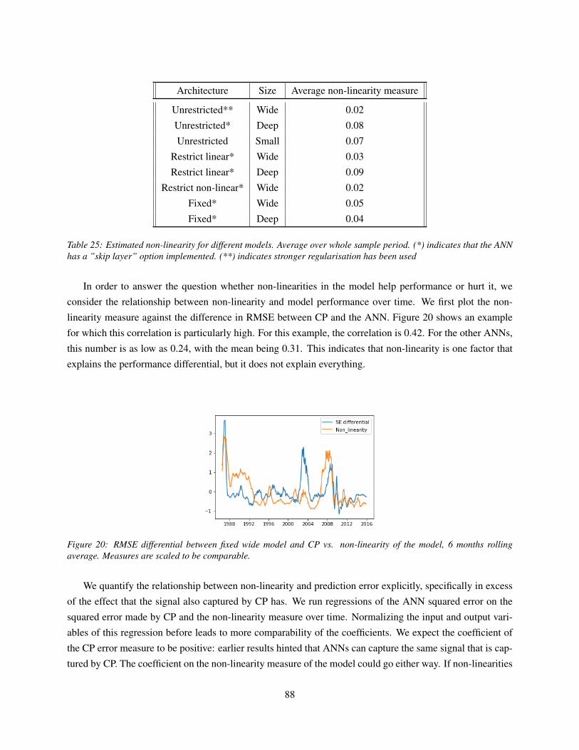
Architecture Size Average non-linearity measure
Unrestricted** Wide 0.02
Unrestricted* Deep 0.08
Unrestricted Small 0.07
Restrict linear* Wide 0.03
Restrict linear* Deep 0.09
Restrict non-linear* Wide 0.02
Fixed* Wide 0.05
Fixed* Deep 0.04
Table 25: Estimated non-linearity for different models. Average over whole sample period. (*) indicates that the ANNhas a ”skip layer” option implemented. (**) indicates stronger regularisation has been used
In order to answer the question whether non-linearities in the model help performance or hurt it, we
consider the relationship between non-linearity and model performance over time. We first plot the non-
linearity measure against the difference in RMSE between CP and the ANN. Figure 20 shows an example
for which this correlation is particularly high. For this example, the correlation is 0.42. For the other ANNs,
this number is as low as 0.24, with the mean being 0.31. This indicates that non-linearity is one factor that
explains the performance differential, but it does not explain everything.
Figure 20: RMSE differential between fixed wide model and CP vs. non-linearity of the model, 6 months rollingaverage. Measures are scaled to be comparable.
We quantify the relationship between non-linearity and prediction error explicitly, specifically in excess
of the effect that the signal also captured by CP has. We run regressions of the ANN squared error on the
squared error made by CP and the non-linearity measure over time. Normalizing the input and output vari-
ables of this regression before leads to more comparability of the coefficients. We expect the coefficient of
the CP error measure to be positive: earlier results hinted that ANNs can capture the same signal that is cap-
tured by CP. The coefficient on the non-linearity measure of the model could go either way. If non-linearities
88

in the data help predict returns, a model that is able to capture non-linearity should, ceteris paribus, lead to
better predictions. If there are no non-linearities in the data that predict excess returns, we would - naively
- expect the ANN model predictions to be equal to the CP predictions. In practice, however, a non-linear
model might fit noise in sample, even if the true relationship is linear. This was demonstrated in the tools
and concepts section and referred to as overfitting. We would thus expect the coefficient on the non-linearity
measure to be positive and significant if non-linearities do not help predicting excess returns: The model will
fit something in the training data, even if it does not help prediction out of sample.
Running the regression described above, we correct standard errors using GMM since we expect the data
to be serially correlated: Overlapping sample periods make an error in one period likely to still have an
effect in the next one as well. By using GMM we furthermore ensure that if there is heteroscedasticity in
the model, we correct for that as well. We find significant coefficients for both the CP squared errors and
the non-linearity measure (Table 26). The coefficients on CP squared errors are all highly significant, while
the ones on the non-linearity measure are all significant at a 5% level, but for one ANN. The linear restricted
wide model is also not significant at a 10% level. The average coefficient on the CP squared error is 0.76
and the average coefficient on the non-linearity measure is 0.2. Since we work with normalized data, we
can compare the coefficients directly. The deep fixed model is the one with the highest coefficient on the
CP squared error, with a value of 0.83. This means that an increase in the CP squared error by one standard
deviation would increase the ANN squared error by 0.83 standard deviations. The wide linear restricted
model also has the lowest coefficient on CP squared error, 0.69, with a similar interpretation as above. The
highest coefficient on the non-linearity measure is displayed by the wide fixed model, with a value of 0.25,
meaning that an increase in the non-linearity measure by one standard deviation would lead to an increase
in ANN squared error of 0.25 standard deviations. The lowest coefficient on the non-linearity measure is
displayed by the wide linear restricted model.
When training the models, we increased the number of training periods by 50% and saved these predic-
tions as well. When doing this, we found a higher degree of non-linearity, accompanied by worse out of
sample performance. This side note shows that the ANNs are able to introduce more non- linearity than we
found if they are trained longer. This however decreases out of sample fit.
Putting the results into context, we find that a higher degree of non-linearity increases the prediction er-
ror in our models when controlling for the errors made by CP. We can thus conclude that the non-linearity in
the models contributes directly to their underperformance relative to CP. From a statistical point of view, CP
thus appears to be the better model, since non-linearity in the model only increases overfitting and a linear
relationship captures the predictive signal better.
89

Economic performance Turning to the economic performance, we conduct analysis along the lines
of the statistical one. First, we calculated the return of going long in the ANN signal while going short
in the signal delivered by CP. Following the same idea, this strategy should give us the return of the non-
linear part of the signal delivered by the ANNs. The returns of this strategy are negative for all ANNs
for a 20 year training window that we investigated. This is in line with what was found in the section on
economic performance and shows that, when isolated, the difference between CP and the ANNs delivers
negative returns. Next, we relate the non-linearity measure we developed to these returns in order to find the
correlation.
Figure 21: Return differential between fixed wide model and CP vs. non-linearity of the model, 12 months rollingaverage. Measures are scaled to be comparable.
Figure 21 shows the returns for the same ANN depicted in Figure 20, one that displays a particularly high
correlation between RMSE and non-linearity measure. We find that this ANN also has the most negative cor-
relation between return differential and non-linearity measure, with a correlation of -0.26. The least negative
correlation is displayed by the small unrestricted network and is only -0.05. On average, the correlation is a
bit weaker than for RMSE and negative, with a value of -0.15. The link between relative underperformance
of the ANNs and non-linearity as measured by us is thus not as clear as for the RMSE. This is not surprising,
given that we trade only on the sign of the prediction which provides a natural cutoff and could make the
relationship between performance differential and non-linearity weaker.
90

Coefficients SE T-stat P-value
β0 CP
SE
RMS
DL
β0 CP
SE
RMS
DL
β0 CP SE RMS
DL
β0 CP
SE
RMS
DL
RMSE
FD* 0 0.8392 0.1777 0.0379 0.0556 0.0700 0 15.093 2.538 1 0 0.0111
FW* 0 0.7472 0.2517 0.0562 0.0468 0.0962 0 15.972 2.616 1 0 0.009
LD* 0 0.7067 0.2447 0.0792 0.0650 0.1199 0 10.872 2.041 1 0 0.0413
LW* 0 0.6895 0.1517 0.0849 0.0632 0.0951 0 10.91 1.595 1 0 0.1107
NW* 0 0.8275 0.1781 0.0416 0.049 0.0674 0 16.888 2.642 1 0 0.0082
UD* 0 0.7658 0.1975 0.061 0.045 0.093 0 17.017 2.124 1 0 0.0337
UW** 0 0.7534 0.2341 0.0619 0.0624 0.1068 0 12.074 2.192 1 0 0.0284
US 0 0.7901 0.1533 0.0575 0.0610 0.0534 0 12.952 2.871 1 0 0.0041
Returns
FD* 0 0.8055 -0.0756 0.0471 0.0664 0.0833 0 12.1308 -0.9072 1 0 0.3643
FW* 0 0.6596 -0.2189 0.0653 0.1130 0.1318 0 5.8370 -1.6607 1 0 0.0968
LD* 0 0.5314 -0.2125 0.0898 0.1430 0.1425 0 3.7162 -1.4912 1 0 0.1359
LW* 0 0.5726 -0.1922 0.0777 0.1267 0.1331 0 4.5192 -1.4438 1 0 0.1488
NW* 0 0.8350 -0.0368 0.0417 0.0527 0.0580 0 15.8445 -0.6347 1 0 0.5256
UD* 0 0.6688 -0.0867 0.0796 0.1211 0.1200 0 5.5227 -0.7226 1 0 0.4699
UW** 0 0.6968 -0.1573 0.0676 0.0847 0.1302 0 8.2267 -1.2080 1 0 0.227
US 0 0.8077 -0.0217 0.0399 0.0485 0.0491 0 16.6543 -0.4419 1 0 0.6586
Table 26: Coefficients, standard errors, t-statistics and p-values for regressions of ANN squared errors and tradingstrategy returns on CP squared errors and trading strategy returns and non-linearity measure. ANN names are ab-breviated as follows: FD means fixed deep, FW fixed wide, US unrestricted wide etc. Standard errors are correctedusing GMM with 12 lags, as described in the Methodology section. RMSDL stands for root mean squared distanceto linear, a non-linearity measure described in the tools and concepts section.(*) indicates ”skip-layer” option wasimplemented. (**) indicates stronger regularisation was used.
Next, we run regressions to single out the relationship between non-linearity and economic underperfor-
mance of ANNs. We find that the non-linearity as measured by us is not significant when controlling for the
CP strategy returns (Table 26). The signs are generally in line with the results that we found when regressing
squared errors on non-linearity.
In summary, we find that the non-linearity provided by the ANN models makes the predictions worse in
a statistical sense. In economic terms, the relationship is not as clear. We suspect that to be due to the cutoff
implemented by the rough trading signal, which could be heavily influenced by outliers in both directions.
7.7 ANN Decomposition
As illustrated, a combination of the CP predictions and our non-linearity score RMSDL explains a large part
of the variation in predictions of the various ANNs. CP is highly significant in all cases, but the significance
91

of the level of non-linearity varies, within (and slightly outside) the range of conventionally significant p-
values. Assuming that CP is the the signal, it is intuitively appealing to expect predictions made by the ANNs
to consist of a linear component close to CP and an additional non-linear component, and that variations in
this component is the driver of variations from the signal. While CP seems hard to beat out of sample
in the category of predictors that manages to capture some of the dynamics of realized excess returns (as
opposed to the unconditional mean), it is at best the best approximation of the signal, and as touched upon
in our discussion of it is possible that it is already a ”bigger” model than what is strictly necessary. As such
deviations from CP may be entirely meaningful, and as it is clear from R2 figures it is actually the case that
the ANNs often are able to obtain an edge here. In this case meaningful has a precise mathematical meaning
as a minimum with a lower error that the optimizer picks for an ANN during training. In a world where the
optimum is a linear combination gradient descent would eventually find the minimum corresponding hereto.
However, this optimum is only the optimum contingent on noise - within a given sample there is an optimum
with a much more involved prediction functions. While different regularization techniques help to make the
optimizer condition on noise in different ways it is likely that the discovered optimum will still consist of
a mix of linear and non-linear features which are jointly optimized. The final point is important because
it reveals weakness in the separation heuristic described above. Because of the interaction between linear
and non-linear features, which may also be close to linear on certain input ranges, there is nothing forcing
a near optimum to consist of a perfect linear part and a deviation term attributable entirely to the non-linear
features. Especially for data where training data and test data exhibits on average exhibits different levels,
small deviations in linear and close to linear weights in sample may translate to bigger difference out of
sample as counterbalances in non-linear weights falls away because of a change in range into a range where
the feature close to inactive or itself acts linearly. In this case, the additional flexibility of allowing for non-
linearity is the source of deviations, but the deviations in predictions won’t be correlated with the level of
non-linearity. Clearly the way non-linearity is measured plays a large role in this, and as discussed in the
section on our measure RMSDL we make a number of choices that could be described as heuristic or even ad
hoc. As our study is not a technical study of a distance measure we will not dig deeper into the properties of
the measure as, but rather trace the contribution to the overall number in ANNs that represents our different
base architectures. Specifically we are interested in whether the restrictions of fixed, linear restricted and
non-linear restricted help us to explain non-linear behaviour.
Fixed In the Fixed ANN, the strictly linear part is fixed to the weights dictated by the CP regression for
the given training data. As these weights by construction represent the linear optimum of the sample at hand
we would by thinking analogous to the separation heuristic described above expect the ANN to only make
non-linear adjustments to this optimum. However, as weights must be randomly initialized14 this heuristic is
a bit too simplistic. We are, however, still interested in whether this relation approximately holds. The Fixed14Training by gradient descent using the chain-rule, initializing all weights to the same value will make all updates to weights
equal meaning that while weights do change the equality between weights does not and the ANN is stuck.
92

ANN we decompose here is the wide15 version.
Linear restricted A main interest in the case of the Linear restricted ANNs, which are restricted to use
only one strictly linear factor for prediction of the four different maturities of excess returns, is whether that
factor recovers the CP tent. The Linear restricted ANN we decompose here is the deep version.
Non-linear restricted In the Non-linear restricted model, the non-linear components are limited to produce
only one output each to the final prediction layer. The limited number of outputs to the prediction layer
forces the ANN to treat each sub-ANN as an individual factor. Comparing the non-linear restricted to other
architectures we can gauge how far other architectures are from this behaviour. For the Non-linear restricted
architecture we discarded the deep version early on, so the ANN considered here is wide.
Unrestricted The Unrestricted category is a bit too broad to raise any specific questions, however, as a
”control” case for the restricted ANNs we briefly look at the small unrestricted ANN without skip-layer.
While the relatively fewer weights in this ANN makes it a bit more tractable, it is also one that is particularly
ill described by RMSDL, and as such a natural candidate for further decomposition.
The decomposition we apply treat the three sub-ANNs (tanh, relu, and sigmoid) and any strictly linear
component individually. They furthermore track the non-linearity score for each part, as well as its output to
the final prediction layer, and the weights assigned to its output in the final prediction layer. From the output
of the sub-ANN and the weights assigned to this output we calculate the contribution to the prediction of the
ANN from each sub-ANN.
Results Table 27 shows that the heuristic of linear optimum vs. non-linear noise is not accurate in that all
the ANNs that include a strictly linear part actually have two strictly linear components: the average RMDSL
for the sigmoid sub-ANN are zero for all three16. From the numbers on average share of absolute contribution
(Table 27) it furthermore becomes clear that this is not because the sigmoid sub-ANN is necessarily shut
down, although the 5% contribution of the component in the Non-linear restricted ANN is practically silence.
In the appendix for this section we include plots of contribution over time for the shortest maturity17 and the
plot for Non-linear restricted illustrates that the role of the sigmoid component in this ANN is negligible.15We refer to the methodology section for elaboration on the terminology we use for our architectures.16Even for the unrestricted ANN where the sigmoid ANN is not strictly linear, it may be playing the more linear part as it is
less non-linear by a factor of 20; but as pointed out in our analytical concepts and tools section it is not clear if such a comparisonis meaningful, as it requires the absolute value of the measure to carry some meaning across set-ups, as opposed to across timecomparing the same set-up to itself.
17the picture is very similar across maturities
93

Avg. share of abs. contr. Avg. non-linearity
Tanh Relu Sigm. Lin. Tanh Relu Sigm. Lin. Full ANN
Fixed 25% 23% 20% 33% 0.0040 0.0063 0.0 0.0 0.0513
Linear restricted 37% 28% 22% 13% 0.0034 0.0085 0.0 0.0 0.0322
Non-linear restricted 21% 21% 5% 53% 0.0171 0.0211 0.0 0.0 0.0232
Unrestricted 51% 22% 27% - 0.0219 0.0216 0.0011 - 0.0667
Table 27: Average share of absolute contribution on the left, average non-linearity of sub-ANNs (RMSDL) on the right.
Digging deeper into what this means for non-linearity, it is natural to ask whether the ANN then treat
the sub-ANNs that contribute non-linearity as a non-linear factor. To get an idea, we look at the correla-
tion between absolute contribution and non-linearity (see Table 28). Among the ANNs surveyed here the
Non-linear restricted comes closest to such behaviour, while both Fixed and Linear restricted directly play
down the contribution of the relu component at times where it is more non-linear. The low correlation for
the Unrestricted ANN may be explained by the absences of a strictly linear part to ’switch’ to.
Finally, to get a feeling for whether specific parts of the ANNs act more as the the core and other parts
as adjustment, we look at the correlation between contribution (in this case not the absolute) and the predic-
tion of the ANN. Fixed 18 seems to come closest to such behaviour with a high correlation between the fixed
strictly linear part and the prediction. The tanh and relu sub-ANNs act more in concert counterbalancing
each other.
Corr. betw. abs. contr. and non-lin. Corr. betw. abs. contr. and Pred.
Tanh Relu Sigmoid Tanh Relu Sigmoid Linear Tanh Relu corr.
Fixed 0.3 -0.35 - 0.32 0.4 -0.17 0.74 -0.39
Linear 0.18 -0.12 - 0.58 0.6 -0.17 0.17 -0.08
Non-linear 0.5 0.46 - 0.17 0.27 0.01 0.54 -0.01
Unrestricted 0.07 0.07 0.09 0.65 0.41 0.02 - -0.08
Table 28: Average correlation between absolute contribution and non-linearity. Average correlation between contri-bution and ANN prediction.
For the more ANN specific hypothesis, it does not seem that Linear restricted recovers the CP tent factor,
whereas the forced separation into ’factors’ of Non-linear restricted has some effect. For the linear restricted
ANN it is, however, evident that both in terms of absolute contribution and correlation with prediction the
strictly linear component does not play a large role for the output produced. This would explain how the
ANN can make predictions relatively similar to CP without recovering the tent factor in the strictly linear18which was build with this separation in mind
94

part.
Figure 22: The linearly restricted layer does not recover the tent factor.
Figure 23: Correlation between absolute contribution and ANN Prediction. Non-linear restricted is only ANN withclear spread between maturities reflecting the distinct separation of non-linearly enabled sub-ANNs.
Two out of the three restrictions we impose to form our architectures seems to have some degree of
the intended effect, however, the main takeaway from decomposing the ANNs further is that the similar
predictions we have documented in previous sections are achieved in quite different ways. We consider this
support for a data- rather than model-driven convergence, i.e. it is the common signal picked up rather than
a common tendency in behaviour that leads the ANNs to make CP-like predictions.
8 Conclusion
In our thesis we extend the empirical work on the Expectation Hypothesis that tests the predictability of
excess returns on default free bonds. Our main reference is the work of Cochrane and Piazzesi (2005) who
find a predictive factor that is a linear combination of five forward rates. In subsequent studies, both lagged
forward rates and different types of macroeconomic information are considered information outside the cur-
rent yield curve that may help predict future excess returns. We cover the link to the theory of affine term
structure models for which these empirical findings have led to two notable extensions: state factor depen-
dent risk premia (Duffee (2002)), and hidden factors (Duffee (2011)). Our hypothesis can be formulated
as a direct extension of the finding of the predictive factor: can a non-linear combination of forward rates
improve the predictability of excess returns compared to a linear combination. A follow up question for our
hypothesis is whether allowing for non-linear relations between forward rates makes the inclusion of outside
information redundant. We conduct our analysis out of sample, essentially extending the approach used by
95

Campbell and Thompson (2008) to bond markets.
Our dataset extends the data used by Cochrane and Piazzesi (2005) to 2015 and includes real-time macroe-
conomic data for the period from 1982. We add to the group of considered predictors by including ANNs,
which contribute the ability to fit non linear relations in the data without assumptions on functional form. We
consider a 20 year sample period to be the most meaningful. We find that the best predictor of future excess
returns is their historical average, providing a 10% decrease in RMSE compared to the next best predictor.
We thus fail to reject the Expectations Hypothesis out of sample. A noisy data generating process may ex-
plain this finding: Predictions made by estimators working well in sample capture the movements of excess
returns better than the mean, while missing the level on average. Predictions made by the linear combination
of forward rates have a correlation of over 0.4 while the mean has a correlation of about −0.17. We do not
find support for non-linear combinations of yields to add any meaningful out of sample predictive power
beyond a simple linear combination of yields. We find instead that Artificial Neural Networks converge on
the same signal recovered by a linear combination of five forward rates, with a correlation of 0.68. If there is
a signal it seems to be a linear combination of yields. This finding supports the state dependent specification
of the market price of risk, with the disclaimer that our failure to reject the Expectations Hypothesis in itself
does not support bond risk-premia at all. Furthermore, we find that neither lagged forward rates nor real time
macroeconomic data add predictive power out of sample. From a theoretical perspective, this means that
even under the signal obscured by noise interpretation discussed above we do not find a hidden factor in the
yield curve.
Additional limitations We have covered uncertainties with regards to our methodology, data, and esti-
mates where relevant. One limitation to our study that has not been addressed is that of the general set-up
we adopt from previous studies: Using US treasuries, considering monthly data, and only including forward
rates and holding period returns based on yields for five maturities.
Focusing on only one economy, albeit a very important one, the data may be overly exposed to noise from
country specific factors such as monetary policy, wars, etc. As researchers have found predictive power in
forwards around the world and across countries (briefly covered in our literature review) it is possible that a
international dataset may provide different results.
Secondly, the approach of estimating yearly holding periods on monthly data is appealing: A three year
bond becoming a two year bond has clearer meaning than a three year bond becoming a two year and eleven
months bond. Retrieving market prices for these ”in-between” maturities is also an issue. Ideally we should
prefer to estimate yearly periods with yearly data, but the length of available time-series inhibits this. An-
other concern beside the length of time-series, however, may be whether some relations are in fact stable
over shorter periods or even changing in ways not entirely unpredictable. It may be that in expanding the
estimation window in order to get more data-points we are including more time noise, favouring less sen-
96

sitive estimators; unconditional mean over conditional, linear over non-linear. As such, combined ways of
better understanding interim bond-prices estimation on daily data may produce other results than the ones
we present here.
Finally, there is the question of how many maturities to include and maybe even more importantly which
interpolations methods to choose. Bliss (1996) finds that different methods of interpolation shows quite dif-
ferent performance in and out of sample, which could be relevant as our results vary so markedly between
the two. For maturities specifically, it is possible that our long bond is not ”long enough” if some variation
is driven by very long horizons.
97
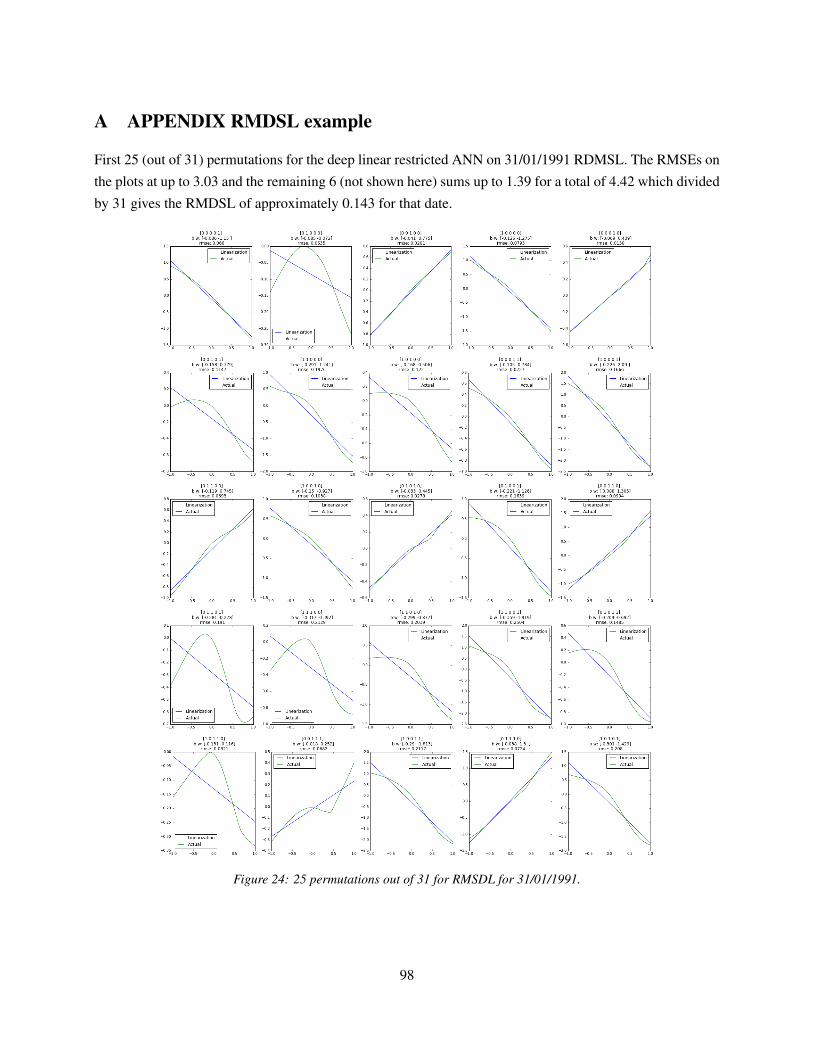
A APPENDIX RMDSL example
First 25 (out of 31) permutations for the deep linear restricted ANN on 31/01/1991 RDMSL. The RMSEs on
the plots at up to 3.03 and the remaining 6 (not shown here) sums up to 1.39 for a total of 4.42 which divided
by 31 gives the RMDSL of approximately 0.143 for that date.
Figure 24: 25 permutations out of 31 for RMSDL for 31/01/1991.
98

B APPENDIX macro dataset
Below is the list of variables contained in the real-time macroeconomic dataset. The latest beginning of any
of the timeseries is the beginning of our dataset.
Description Date Begin
All Employees: Manufacturing 01/11/1964
Housing Starts: 2-4 Units 01/02/1973
Producer Price Index: Finished Consumer Foods 01/01/1982
Producer Price Index: Finished Consumer Goods Excluding Foods 01/01/1982
Producer Price Index: Crude Foodstus&Feedstus 01/01/1982
Producer Price Index: Finished Goods 01/01/1982
Producer Price Index: Intermediate Foods & Feeds 01/01/1982
Civilians Unemployed for 15-26 Weeks 2 1/1/1982 01/01/1982
Median Duration of Unemployment 01/01/1982
Total Checkable Deposits 03/01/1981
Other Checkable Deposits 02/01/1981
Real Personal Consumption Expenditures 03/01/1980
Real Personal Consumption Expenditures: Durable Goods 03/01/1980
Real Personal Consumption Expenditures: Nondurable Goods 03/01/1980
Real Personal Consumption Expenditures: Services 03/01/1980
Real Disposable Personal Income 02/01/1980
Disposable Personal Income 01/01/1980
M1 Money Stock 12/01/1979
M2 Money Stock 12/01/1979
Personal Consumption Expenditures 12/01/1979
Personal Consumption Expenditures: Durable Goods 12/01/1979
Personal Consumption Expenditures: Nondurable Goods 12/01/1979
Personal Consumption Expenditures: Services 12/01/1979
Savings Deposits - Total 12/01/1979
Small Time Deposits at Commercial Banks 12/01/1979
Small Time Deposits - Total 12/01/1979
Small Time Deposits at Thrift Institutions 12/01/1979
Savings Deposits at Commercial Banks 12/01/1979
Savings Deposits at Thrift Institutions 12/01/1979
Savings and Small Time Deposits at Commercial Banks 12/01/1979
Savings and Small Time Deposits - Total 12/01/1979
99

Description Date Begin
Producer Price Index: Crude Materials for Further Processing 03/01/1978
Producer Price Index: Intermediate Materials: Supplies & Components 03/01/1978
Producer Price Index: Finished Goods: Capital Equipment 01/01/1978
Consumer Price Index for All Urban Consumers: All Items 06/01/1972
Privately Owned Housing Starts: 1-Unit Structures 02/01/1972
Average (Mean) Duration of Unemployment 01/01/1972
All Employees: Service-Providing Industries 09/01/1971
All Employees: Goods-Producing Industries 09/01/1971
All Employees: Total Private Industries 08/01/1971
Average Weekly Hours Of Production And Nonsupervisory Employees: Total private 05/01/1970
Average Weekly Overtime Hours of Production and Nonsupervisory Employees: Manufacturing 08/01/1966
Personal Income 02/01/1966
Civilians Unemployed for 27 Weeks and Over 01/01/1966
Civilian Employment 12/01/1964
Housing Starts: Total: New Privately Owned Housing Units Started 12/01/1964
Unemployed 12/01/1964
All Employees: Construction 12/01/1964
All Employees: Financial Activities 12/01/1964
All Employees: Government 12/01/1964
All Employees: Mining and logging 12/01/1964
All Employees: Other Services 12/01/1964
All Employees: Trade, Transportation & Utilities 12/01/1964
All Employees: Retail Trade 12/01/1964
All Employees: Wholesale Trade 12/01/1964
Average Weekly Hours of Production and Nonsupervisory Employees: Manufacturing 11/01/1964
Civilian Labor Force 11/01/1964
Currency Component of M1 Plus Demand Deposits 11/01/1964
Currency Component of M1 11/01/1964
All Employees: Durable goods 11/01/1964
Industrial Production Index 11/01/1964
All Employees: Nondurable goods 11/01/1964
All Employees: Total nonfarm 11/01/1964
Civilians Unemployed - 15 Weeks & Over 11/01/1964
Civilians Unemployed for 5-14 Weeks 11/01/1964
Civilians Unemployed - Less Than 5 Weeks 11/01/1964
Demand Deposits at Commercial Banks 09/01/1964
Civilian Unemployment Rate 02/01/1960
100

C APPENDIX ANN decomposition
Figure 25: Contribution to ANN prediction, and non-linearity scores for sub-ANNs as well as full ANN for the Fixedand Linear restricted architectures.
101

Figure 26: Contribution to ANN prediction, and non-linearity scores for sub-ANNs as well as full ANN for the Non-linear restricted and Unrestricted architectures.
102

D APPENDIX Technical details
This section is not central to understanding any part of the thesis, but is provided for full transparency and to
cite technical sources. It can be considered and extended READ-ME for the code examples included in the
digital submission.
Our language of choice for this thesis is Python. Especially the Keras library for Deep learning Chol-
let (2015) is central for our estimation of ANNs as it provides the degree of control that is suitable for our
purposes as an interface to Google’s TensorFlow Abadi et al. (2015). A library that is configured for the
usage of Graphical Processor Units (GPU), which is very efficient for the large matrix operations that are
required in training ANNs. On top of that, Python offers a strong base for scientific computing via packages:
Numpy by Walt, Colbert, and Varoquaux (2011), the name is short for numerical python; Pandas McKin-
ney (2010) adds a layer of data-frame functionality to Numpy; and Matplotlib Hunter (2007) a library for
plotting. Finally, Python is a dynamical and interpreted language, which means it can run interactively19.
This functionality inspired the creation of the environment Jupyter Notebook (formerly IPython Perez and
Granger (2007)), which represent an interactive session in the browser, and makes running blocks of code
rather than full scripts, writing commentary for specific sections, and viewing output, straight forward. The
code examples we include are such notebooks exported to html, which means they can viewed in any modern
browser without requiring Python or any of the packages described above as all relevant code has been run
before export. A feature of the Jupyter notebook that is not important in normal usage, but comes in handy
for our purposes, arises from hosting the session in the browser. The feature in question is the option to
control the kernel which runs the code through embedded JavaScript run by the browser. What we find is
that as when we train 360-480 models (one for each period) to perform rolling predictions with an ANN,
the kernel slows down after 20-40 runs. By embedding code to restart the kernel automatically we speed up
training of an ANN on the full period form about 6 hours to about 20 minutes. We use this code again for
calculating non-linearity scores for the stored models. Because the kernel restart we cannot save variables in
scope and we write to file to control the restarting and stop when we are through our dataset.
In one case we case we use R, as we find the sandwich package Zeileis (2004) more intuitive for calcu-
lating Hansen-Hodrick errors i.e. GMM standard errors than equivalents we could find for Python.19Other languages often applied in statistical analysis such as R and Matlab are also dynamic languages, but popular more
’production environment’ languages C++ and Java are not.
103

References
Abadi, Martın et al. (2015). TensorFlow: Large-Scale Machine Learning on Heterogeneous Systems. Soft-
ware available from tensorflow.org. URL: http://tensorflow.org/.
Abu-Mostafa, Yaser S., Malik Magdon-Ismail, and Hsuan-Tien Lin (2012). Learning from Data.
Ang, Andrew and Monika Piazzesi (2003). “A no-arbitrage vector autoregression of term structure dynamics
with macroeconomic and latent variables”. In: Journal of Monetary Economics 50(4), pp. 745–787.
Bekaert, Geert and Robert J. Hodrick (2001). “Expectations hypotheses tests”. In: Journal of Finance 56(4),
pp. 1357–1394.
Bjork, Tomas (2009). Arbitrage Theory in Continuous Time. 3rd ed. Oxford University Press.
Black, Fischer and Myron Scholes (1973). “The pricing of options and corporate liabilities”. In: Journal of
political economy 81(3), pp. 637–654.
Bliss, Robert R (1996). Testing term structure estimation methods. Tech. rep. Working paper, Federal Reserve
Bank of Atlanta.
Bollen, Nicolas PB et al. (1997). “Derivatives and the price of risk”. In: Journal of Futures Markets 17(7),
pp. 839–854.
Campbell, John Y (1986). “A defense of traditional hypotheses about the term structure of interest rates”. In:
The Journal of Finance 41(1), pp. 183–193.
Campbell, John Y. (1987). “Stock returns and the term structure”. In: Journal of Financial Economics 18(2),
pp. 373–399.
Campbell, John Y and Yasushi Hamao (1992). “Predictable stock returns in the United States and Japan: A
study of long-term capital market integration”. In: The Journal of Finance 47(1), pp. 43–69.
Campbell, John Y and Robert J Shiller (1991). “Yield spreads and interest rate movements: a bird’s eye
view”. In: The Review of Economic Studies 58(3), p. 495.
Campbell, John Y. and Samuel B. Thompson (2008). “Predicting excess stock returns out of sample: Can
anything beat the historical average?” In: Review of Financial Studies 21(4), pp. 1509–1531.
Chollet, Francois et al. (2015). Keras. https://github.com/fchollet/keras.
Cochrane, John H (2009). Asset Pricing (Revised Edition). Princeton university press.
Cochrane, John H and Christopher L Culp (2003). “Equilibrium asset pricing and discount factors: Overview
and implications for derivatives valuation and risk management”. In: Modern risk management: A history
2.
Cochrane, John H. and Monika Piazzesi (2005). “Bond risk premia”. In: American Economic Review 95(1),
pp. 138–160.
Cochrane, John H and Monika Piazzesi (2008). “Decomposing the Yield Curve”. In: Graduate School of
Business University of Chicago Working Paper, pp. 138–160.
Connect, a. K., a. Krogh, and J. a. Hertz (1992). “A Simple Weight Decay Can Improve Generalization”. In:
Advances in Neural Information Processing Systems 4, pp. 950–957.
104

Coroneo, Laura, Domenico Giannone, and Michele Modugno (2016). “Unspanned Macroeconomic Factors
in the Yield Curve”. In: 34(3), pp. 472–485.
Cox, John, Jonathan Ingersoll, and Stephen Ross (1981). “A Re-examnation of Traditional Hypotheses about
the Term Structure of Interest Rates”. In: Journal of Finance 36(4), pp. 769–799.
Cox, John C, Jonathan E Ingersoll, and Stephen A Ross (1985). “A Theory of the Term Structure of Interest
Rates”. In: Econometrica 53(2), pp. 385–407.
Dahlquist, Magnus and Henrik Hasseltoft (2013). “International Bond Risk Premia”. In: Journal of Interna-
tional Economics 90(1), pp. 17–32.
Dai, Qiang and Kenneth J. Singleton (2000). “Specification Analysis of Affine Term Structure Models”. In:
The Journal of Finance 55(5), pp. 1943–1978.
Dai, Qiang and Kenneth J Singleton (2002a). “Expectation puzzles, time-varying risk premia, and affine
models of the term structure”. In: Journal of financial Economics 63(3), pp. 415–441.
Dai, Qiang and Kenneth J. Singleton (2002b). “Expectation puzzles, time-varying risk premia, and affine
models of the term structure”. In: Journal of Financial Economics 63(3), pp. 415–441.
Dietterich, Thomas G. (2000). “Ensemble Methods in Machine Learning”. In: Multiple Classifier Systems:
First International Workshop, MCS 2000 Cagliari, Italy, June 21–23, 2000 Proceedings. Springer Berlin
Heidelberg: Berlin, Heidelberg, pp. 1–15.
Duchi, John, Elad Hazan, and Yoram Singer (2011). “Adaptive subgradient methods for online learning and
stochastic optimization”. In: Journal of Machine Learning Research 12(Jul), pp. 2121–2159.
Duffee, Gregory R. (2002). “Term premia and interest rate forecasts in affine models”. In: Journal of Finance
57(1), pp. 405–443.
Duffee, Gregory R. (2011). “Information in (and not in) the term structure”. In: Review of Financial Studies
24(9), pp. 2895–2934.
Duffie, Darrell and Rui Kan (1996). “A Yield-Factor Model of Interest Rates”. In: Mathematical Finance
6(4), pp. 379–406.
Fama, Eugene F and Robert R Bliss (1987). “The Information in Long-Maturity Forward Rates”. In: The
American Economic Review 77(4), pp. 680–692.
Fan, Hua and Suresh M Sundaresan (2000). “Debt valuation, renegotiation, and optimal dividend policy”.
In: Review of financial studies 13(4), pp. 1057–1099.
Feldhutter, P, Christian Heyerdahl-Larsen, and Philipp Illeditsch (2013). Risk Premia, Volatilities, and Sharpe
Ratios in a Nonlinear Term Structure Model. Tech. rep. Discussion paper, London Business School and
the Wharton School.
Ghysels, Eric, Casidhe Horan, and Emanuel Moench (2014). “Forecasting Through the Rear-View Mirror:
Data Revisions and Bond Return Predictability”. In: Federal Reserve Bank of New York Staff Reports
581(March).
Hamey, L.G.C. (1998). “XOR has no local minima: A case study in neural network error surface analysis”.
In: Neural Networks 11(4), pp. 669–681.
105

Hansen, Lars Kai and Peter Salamon (1990). “Neural network ensembles”. In: IEEE transactions on pattern
analysis and machine intelligence 12(10), pp. 993–1001.
Hansen, Lars Peter (1982). “Large sample properties of generalized method of moments estimators”. In:
Econometrica: Journal of the Econometric Society, pp. 1029–1054.
Heaton, J. B., N. G. Polson, and J. H. Witte (2016). “Deep Learning in Finance”. In: 2, p. 06561.
Hellerstein, Rebecca (2011). “Global Bond Risk Premiums”. In: SSRN Electronic Journal.
Hicks, John Richard (1946). “Value and capital, 1939”. In: Mathematical Appendix, pp. 311–2.
Hochreiter, Sepp (1998). “The Vanishing Gradient Problem During Learning Recurrent Neural Nets and
Problem Solutions”. In: International Journal of Uncertainty, Fuzziness and Knowledge-Based Systems
06(02), pp. 107–116.
Hunter, J. D. (2007). Matplotlib: A 2D graphics environment.
Ilmanen, Antti (1995). “Time-varying expected returns in international bond markets”. In: The Journal of
Finance 50(2), pp. 481–506.
Joslin, Scott, Kenneth J. Singleton, and Haoxiang Zhu (2011). “A new perspective on gaussian dynamic term
structure models”. In: Review of Financial Studies 24(3), pp. 926–970.
LeCun, Yann A. et al. (2012). “Efficient backprop”. In: Lecture Notes in Computer Science (including sub-
series Lecture Notes in Artificial Intelligence and Lecture Notes in Bioinformatics) 7700 LECTU, pp. 9–
48.
Liaw, a and M Wiener (2002). “Classification and Regression by randomForest”. In: R news 2(December),
pp. 18–22.
Litterman, Robert B and Jose Scheinkman (1991). “Common factors affecting bond returns”. In: The Journal
of Fixed Income 1(1), pp. 54–61.
Lo, Andrew W and a. Craig Mackinlay (1997). “Maximizing Predictability in the Stock and Bond Markets”.
In: Macroeconomic Dynamics 1(01), pp. 102–134.
Ludvigson, Sydney C. and Serena Ng (2009). “Macro factors in bond risk premia”. In: Review of Financial
Studies 22(12), pp. 5027–5067.
Lutz, F A (1940). “The Structure Of Interest Rates”. In: Quarterly Journal of Economics 55(1), pp. 36–63.
Macaulay, Frederick R (1938). “Some theoretical problems suggested by the movements of interest rates,
bond yields and stock prices in the United States since 1856”. In:
McKinney, Wes (2010). Data Structures for Statistical Computing in Python. Ed. by Stefan van der Walt and
Jarrod Millman.
Merton, Robert C (1973). “Theory of rational option pricing”. In: The Bell Journal of economics and man-
agement science, pp. 141–183.
Miersemann, Erich (2012). “Partial Differential Equations Lecture Notes”. In:
Nelson, Charles R. and Andrew F. Siegel (1987). “Parsimonious Modeling of Yield Curves”. In: The Journal
of Business 60(4), pp. 473–489.
106

Neuneier, Ralph and Hans Georg Zimmermann (2012). “How to train neural networks”. In: Lecture Notes
in Computer Science (including subseries Lecture Notes in Artificial Intelligence and Lecture Notes in
Bioinformatics) 7700 LECTURE NO, pp. 369–418.
Perez, Fernando and Brian E. Granger (2007). IPython: a System for Interactive Scientific Computing. DOI:
10.1109/MCSE.2007.53. URL: http://ipython.org.
Piazzesi, Monika (2010). “Affine term structure models”. In: Handbook of financial econometrics 1, pp. 691–
766.
Sangvinatsos, A (2010). “Expectations Hypothesis”. In: Encyclopedia of Quantitative Finance.
Sarno, Lucio, Daniel L. Thornton, and Giorgio Valente (2007). “The Empirical Failure of the Expectations
Hypothesis of the Term Structure of Bond Yields”. In: Journal of Financial and Quantitative Analysis
42(01), pp. 81–100.
Sharpe, William F. (1994). “The Sharpe Ratio”. In: The journal of Portfolio Management 21(1), pp. 49–58.
Stock, James and Mark W. Watson (2002a). “Forecasting Using Principal Components from a Large Number
of Predictors”. In: Journal of the American Statistical Association 97(460), pp. 1167–1179.
Stock, James H and Mark W Watson (2002b). “Macroeconomic Forecasting Using Diffusion Indexes”. In:
Journal of Business & Economic Statistics 20(2), pp. 147–162.
Strang, Gilbert (1991). Calculus, Wellesley.
Towell, Geoffrey G and Jude W Shavlik (1993). “Extracting refined rules from knowledge-based neural
networks”. In: Machine Learning 13(1), pp. 71–101.
Vasicek, Oldrich (1977). “An equilibrium characterization of the term structure”. In: Journal of Financial
Economics 5(2), pp. 177–188.
Vidal, Rene, Yi Ma, and Shankar Sastry (2016). Generalized principal component analysis.
Walt, Stefan van der, S. Chris Colbert, and Gael Varoquaux (2011). The NumPy Array: A Structure for
Efficient Numerical Computation. Piscataway, NJ, USA. DOI: 10.1109/MCSE.2011.37. URL:
http://dx.doi.org/10.1109/MCSE.2011.37.
Winkler, David A and Tu C Le (2017). “Performance of Deep and Shallow Neural Networks, the Universal
Approximation Theorem, Activity Cliffs, and QSAR”. In: Molecular Informatics 36(1-2), 1600118–n/a.
Wu, Liuren and Frank Xiaoling Zhang (2008). “A No-Arbitrage Analysis of Macroeconomic Determinants
of the Credit Spread Term Structure”. In: Management Science 54(6), pp. 1160–1175.
Ye, Jianming (1998). “On Measuring and Correcting the Effects of Data Mining and Model Selection On
Measuring and Correcting the Effects of Data Mining and Model Selection”. In: American Statistical
Association 93(441), pp. 120–131.
Zeileis, Achim (2004). “Econometric Computing with HC and HAC Covariance Matrix Estimators”. In:
Journal of Statistical Software 11(10), pp. 1–17. URL: http://www.jstatsoft.org/v11/i10/.
107