uml - university of hawaii at manoa · 2014-06-13 · 4.1 monthly average co2 concentration in dry...
TRANSCRIPT

INFORMATION TO USERS
This manuscript has been reproduced from the microfilm master. UMIfilms the text directlyfrom the original or copy submitted. Thus, somethesis and dissertation copies are in typewriter face, while others maybe from any type of computerprinter.
The quality or this reproduction is dependent upon the quality or thecopy submitted. Broken or indistinct print, colored or poor qualityillustrations and photographs, print bleedthrough, substandard margins,and improper alignment can adversely affect reproduction.
In the unlikely event that the author did not send UMI a completemanuscript and there are missing pages, these will be noted. Also, ifunauthorized copyright material had to be removed, a note will indicatethe deletion.
Oversize materials (e.g., maps, drawings, charts) are reproduced bysectioning the original, beginning at the upper left-hand comer andcontinuing from left to right in equal sections withsmall overlaps. Eachoriginal is also photographed in one exposure and is included inreduced form at the back of the book.
Photographs included in the originalmanuscript have been reproducedxerographically in this copy. Higher quality 6" x 9" black and whitephotographic prints are available for any photographs or illustrationsappearing in this copy for an additional charge. Contact UMI directlyto order.
UMlUniversity Microfilms International
A Bell &Howell tntormanon Company300 North Zeeb Road. Ann Arbor. MI48106·1346 USA
313/761-4700 800:521·0600


SEA LEVEL RISEAND COASTAL EROSION
IN THE HA~IIAN ISLANDS
A DISSERTATION SUBMITTED TO THE GRADUATE DIVISION OF THEUNIVERSITY OF HAWAII IN PARTIAL FULFILLMENT OF THE
REQUIREMENTS FOR THE DEGREE OF
DOCTOR OF PHILOSOPHY
IN
OCEAN ENGINEERING
MAY 1995
By
Dongchull Jeon
Dissertation Committee:
Franciscus Gerritsen, ChairpersonCharles H. Fletcher III
Edward D. StroupHans-Jurgen Krock
Kwok Fai Cheung

OMI Number: 9532594
OMI Microform 9532594Copyright 1995, by OM! Company. All rights reserved.
This microform edition is protected against unauthorizedcopying under Title 17, United States Code.
UMI300 North Zeeb RoadAnn Arbor, MI 48103

ACKNOWLEDGEMENTS
I wish to thank Prof. Franciscus Gerritsen for g~v~ng
me the chance to synthesize both scientific and engineeringaspects of the oceans. without his invaluable advice andguidance that he has given me throughout the years of mystay at Dept. of Ocean Engineering, Univ. of Hawaii, thisstudy could not have been made.
I also wish to thank the following who deserve myheartful gratitude:
To my other committee members Drs. C. Fletcher, H. Krock, E.Stroup, and K.F. Cheung for giving me important suggestionsto improve my manuscript.
To Dr. Klaus Wyrtki for teaching me the essence about aphysical oceanographer's attitude and intuition.
To Dr. Charles Bretschneider for encouraging me to getfruitful results throughout my study.
To Mr. P. Caldwell at TOGA Sea Level Center, Univ. of Hawaiifor offering me sea-level and wave data and computerprogramming which are the primary essence of this study.
To Dr. N. Wang for cordially offering me his computerprogram to strengthen this study in a modelling aspect.
Most especially to my dear wife, for I could not havecontinued and enjoyed my study without her enduring loveand encouragement.
iii

ABSTRACT
Time series and the power spectral distributions of
relative sea levels are analyzed at selected tide-gauge
stations in the western and central North Pacific between
equator and about 30~, in association with different time
scales of motions. Coastal response to these sea-level
dynamics is discussed in detail, based on the aerial
photographs of shoreline changes. Wave climate around the
Hawaiian Islands as well as surf conditions on Oahu are
examined for simulating cross-shore beach erosion processes
with an energetics-based sediment transport model.
Long-term trend of relative sea-level rise during the
past several decades (+1 to +5 em/decade at most of the
tide-gauge stations) is primarily affec~ed by the local
tectonism such as volcanic loading, plate movement and reef
evolution, and subduction at the plate boundaries.
Continual volcanic loading at Kilauea, Hawaii results in
consequential subsidence of the Hawaiian Islands. Secondary
reason for sea-level rise is the thermal expansion of sea
surface waters due to global warming by increasing
greenhouse gases, which may be potentially more significant
in the near future.
iv

Interannual sea-level fluctuations, associated with
ENSO (El Nino Southern Oscillation) phenomena, seem to be
the primary factor to cause serious beach erosion (up to 10
times the long-term trend). Mean annual cycle of sea level
(H =10 em) and alternate annual wave conditions are the
main causes of the cross-shore oscillation of sediment
transport, although there is still some loss of sediments to
deep-water region.
Short-term change of beach profiles is basically caused
by incoming wave conditions as well as sea-level height,
sediment characteristics, and underlying geology.
Simulations by a cross-shore sediment transport model show
that higher waves result in faster offshore transport and
deeper depth of active profile change, and that beach
recovery process is usually much slower than the erosion
process, especially after a storm surge. Deep erosion
during a storm surge can not be recovered for much longer
duration by mild post-storm waves, but may be partly
recovered by non-breaking long waves such as longer-period
swells.
v

TABLE OF CONTENTS
ACKH01fLEDGEME~S ....................................... iii
ABS~RAC~ •••••••••••••••••••••••••••••••••••••••••••••••• i v
LIST OF TABLES • • • • • 0 • • • • • • • • • • • • • • • • • • • • • • • • • • • • • • • • • • viii
LIST OF FIGURES • • • • • 0 • • • • • • • • • • • • • • • • • • • • • • • • • • • • • • • • • • • x
LIST OF ABBREVIATIONS AND SYMBOLS ..................... xiii
1. InRODUC~IOR ••••••••••••••••••••••••••••••••••••••••• 1
2. SEA-LEVEL RISE IN THE HAWAIIAN ISLANDS
3. METHODS AND ANALYSES
................................................
17
36
...•....••..•.....••..•...•...••.•3.1., AVAILABLE DATA
3.1.1. Tide-gauge Records
3.1.2. Aerial Photographs
......................
......................
36
36
41
3 •1. 3. Waves ................................... 47
3.1.4. Beach and Sediment Characteristics
........................................3.2.1. Mean Sea Levels .........................
54
54
54
53
.......Filling Gaps in MSL Data3.2.1.1.
METHODS3.2.
3.2.1.3. Averaging and Smoothing
3.2.1.2. Linear Regression ......................
56
56
3.2.1.4. Spectral Analyses .............. 57
EFFECTS OF SEA-LEVEL CHARGE ON BEACH EROSION
••••••• e ••••••••••• o •••• " •••••••••
4.
3.3.
3.2.2. Models
ANALYSES OF SEA-LEVEL CHANGES ...........................
58
59
68
vi.

5. EFFEC~S OF S~ORMS OR BEACH EROSION ••••••••••••••••••• 82
6. SHORELINE CHARGES AND BEACH RECOVERY
82
97
107
115
115
122
122
136
147
160
161
163
165
167
.....
• • • 0 • • • • • • • • • • • •
........................................
........................
.........................
............................
................................
• • • • • • • • • • • • • • • • • • • • • • • • • • ~ • G • • •
................................
..................................
• • • • • • • • • • • • • • • • • • • • • • • • G • • • • • • • • • • • • • • • •
GENERAL REMARKS
SHORT-TERM BEACH EROSION MODELS
SHORT-TERM FLUCTUATION
ARTIFICIAL NOURISHMENT
HARD SOLUTIONS
MANAGEMENT STRATEGIES
SHORELINE CHANGES IN THE HAWAIIAN ISLANDS
CASE STUDIES
6.2.1. Waimea Bay Beach, Oahu •••••••••••••••••
6.2.2. Hapuna Beach, Hawaii •••••••••••••••••••
BEACH RECOVERY
5.1.
5.2.
5.3.
6.l.
6.2.
6.3.
7.l.
7.2.
7.3.
8. CONCLUSIONS
7. COASTAL ZORE MARAGEMEftS
APPENDICES. • • • • • • • • • • • • • • • • • • • • • • • • • • • • • • • • • • • • • • • • • • • •• 173
REFERENCES ............................................. 181
vii

LIST OF TABLES
1.1 Estimated contributions to sea level rise ••••••••• 12
2.1 Lengths of the coastlines and the beaches inthe major Hawaiian Islands •••••••••••••••••••••••• 18
2.2 Sea-level trend of rise in the Hawaiian Islands ••• 29
2.3 Projected sea-level rise in 2040 in the HawaiianIslands ..•......................................... 30
2.4 Mean monthly sea-level values and standard deviationsof the annual cycles in the Hawaiian Islands •••••• 31
3.1 Locations and lengths of tide-gauge data atselected island stations in the North Pacific ••••• 37
3.2 Locations and numbers of measured transects ofaerial photographs in major Hawaiian Islands •••••• 42
3.3 The mean sea-level differences of the annual and
interannual oscillations and the rate of sea-levelrise in the Hawaiian Islands •••••••••••••••••••••• 60
5.1 Average wave heights and periods for different
seasons and for different wave types •••••••••••••• 91
6.1 Average sediment size at Waimea Bay Beach, Oahuand at Hapuna Beach, Hawaii •••••••••••••••••••••• 124
6.2 Average sediment size of Hawaiian beach sands
during winter and during summer •••••••••••••••••• 125
6.3 Changes of vegetation line from aerial photos
and converted values with annual cycle of MSL .... 125
6.4 Interannual rising trends of sea-level at Honolulu
Harbor, Oahu 12 B
6;5 Interannual rising trends of sea level at Hilo ••• 139
viii

.....6.6 Volume transports from measured beach profiles
on Waimea Bay, Oahu and Hapuna Beach, Hawaii
6.7 Contributions of sea-level changes and waves
142
to the shoreline retreat ••••••••••••••••••••••••• 158
6.8 Calculated shoreline retreat for different beach-faceslopes .....•...••....................••....•..... 159
A.I Temperature-dependency of the density of standardseawater at an atmospheric pressure •••••••••••••• 174
A.2 Mean annual trends of shoreline changes in theHawaiian Islands •••••••••••••••••••.•••...••••••• 175
ix

LIST OF FIGURES
1.1 Global mean temperature variations on threedifferent time scales since Pleistocene •••••••••••• 3
1.2 Southern oscillation index with annual meanatmospheric pressure, and schematic diagrams ofthe air-sea coupling before and during El Nino •••• 5
1.3 Tilting of the Philippine Islands indicated by
relative land movement at 6 tide-gauge stations •••• 7
1.4 Concentrations of greenhouse gases ••••••••••••••••• 9
1.5 Predicted increase in global mean temperature andsea-level rise ••••••••••.••.••••••••••••••••.•••• 11
2.1 Percentage of the trade winds as monthlyaverages from ship's observations ••••••••••••••••• 23
2.2 Long-term sea level trend, l2-month running
mean, monthly sea levels in the Hawaiian Islands ••• 24
2.3 Model for island development on the Pacific
plate 8 •••••••••••••••••••••••••• 28
2.4 Power spectral density distributions of sea
levels in the Hawaiian Islands •••••••••••••••••••• 33
3.1 Standard deviation of monthly sea level differences
as a function of distance in the Hawaiian Islands,and a time series of monthly sea level anomaliesat Honolulu and Mokuoloe, Oahu •••••••••••••••••••• 40
3.2 Locations of the selected tide-gauge stations,
NOAA wave buoy (51001), and Waimea Bay Beach inOahu and Hapuna Beach in Hawaii ••••••••••••••••••• 48
x

3.3 Example of time series with low frequency
drift and the spectrum of the record •••••••••••••• 52
3.4 Example of Weight-Folding Method for a time-series
of monthly sea levels with a gap of 11 months ••••• 55
3.5 Long-term trend, 12-month running mean, and
monthly sea levels at Truk, Kwajalein, Wake ••••••• 62
3.6 Mean annual cycles of monthly sea levels in
the selected western Pacific islands •••••••••••••• 66
4.1 Monthly average CO2 concentration in dry air
observed at Mauna Loa, Hawaii, and relative
trend of global mean temperature •••••••••••••••••• 69
4.2 Schematic diagram of the relationship between sealevel rise and coastal erosion by Bruun Rule •••••• 71
5.1 Schematic diagram of cross-shore sedimenttransport under waves ••••••••••••••••••••••••••••• 82
5.2 Ranges and mean directions of the typical windwaves around the Hawaiian Islands ••••••••••••••••• 86
5.3 Surf height distributions on Oahu during
winter and summer •••..••.•••••.••••••.•.•.••••••.• 88
5.4 Deep water wave climate as annual variations ofwave height at the northwest of Kauai ••••••••••••• 90
5.5 Location of the points of origin of tropicalcyclones during a 20-year period •••••••••••••••••• 94
5.6 Hurricane tracks around the Hawaiian Islands •••••• 96
5.7 Schematic diagram of Edelman's model for idealized
beach profile, and the relationship between
dune erosion and storm surge height
xi
• • • • • • • • • • • • • D 106

5.8 Relative wave height for a slow-moving hurricaneand components of the storm surge •••••••••••••••• 108
5.9 Schematic diagram of maximum potential responseof equilibrium profile to sea level rise ••••••••• 111
5.10 Amplitude and phase lag of maximum erosionfor different scales of erosion time ••••••••••••• 114
6.1 Mean annual trends of shoreline changes fromaerial photos in the Hawaiian Islands •••••••••••• 118
6.2 Mean annual cycles of monthly sea levels in
the Hawaiian Islands ............................. 120
6.3 Geography and bottom topography of Waimea Bay •••• 123
6.4 Beach profile changes and cross-shore transportrates on Waimea Bay Beach during winter •••••••••• 133
6.5 Beach profile changes and cross-shore transportrates on Waimea Bay Beach during summer •••••••••• 134
6.6 Geography and bottom topography of Hapuna Bay • • • It 137
6.7 Beach profile changes and cross-shore transportrates for different waves on Hapuna Beach ........ 143
6.8 Schematic diagram of complex wave breaking overlong reef bottom in the Hawaiian Islands ••••••••• 147
6.9 Beach profile changes and cross-shore transportrates after storm surge on Waimea Bay Beach •••••• 150
6.10 Beach profile changes and cross-shore transport
rates after storm surge on Hapuna Beach •••••••••• 151
6.11 Seasonal fluctuations in beach sand reservoirsfor selected beaches in the Hawaiian Islands •••••. 153
xii

LIST OF ABBREVIATIONS AND SYMBOLS
ABBREVIATIONS
DWL
ENSO
FFT
HWL
IPCC
MLLW
MSL
NEC
NECC
NOAA
NODC
PSMSL
RSL
TOGA
WFM
Design Water Level
El Nino - Southern Oscillation
Fast Fourier Transform
High Water Line
Intergovernmental Panel on Climate Change
Mean Lower Low Water
Mean Sea Level
North Equatorial Current
North Equatorial Counter Current
National Oceanic and Atmospheric Administration
National Oceanographic Data Center
Permanent Service for Mean Sea Level
Relative Sea Level
Tropical Ocean Global Atmosphere Program
Weight Folding Method
xiii

SYMBOLS
A, A(t) shape parameter in Dean's function
B berm height
c phase speed of waves
Co reference concentration of suspended sedimentat the bottom
Cd sediment concentration at mean water level
CD' CL drag coefficient of beach bottom
Dso, D9 0 characteristic sediment diameter(indices are for mass percentages)
de closure depth with a seaward limit to extremesurf-related effects throughout a typical year
D. displacement error due to radial distortion
Dt displacement error due to tilt
f focal length of camera lens
Fdu g drag force
g gravity
GB sediment-budget terms including sources and sinks
H, Ho deep-water (significant) wave height
Hsso median annual significant wave height
h, hb water depth (index b for wave breaking)or ground elevation of an object on an aerialphotograph
I immersed weight (= weight - buoyancy of fluid)
k wavenumber
K arbitrary number in Dean's wave-sediment parameter
L horizontal distance of active profile zone
xiv

L o
m
M
p
r
R
R(t)
R.
Re
Ru
aqt
< >
S
T
Tc
T.
U
U3* , U/
U t
Um, Um2
U", UL
Wo
W"
deep-water wavelength (= l)
linear beach-face slope (= tan ~)
mass flux between wave crest and trough
pressure or decimal fractioneroded material in the Bruun Rule
distance between isocenter of a photograph andthe point
shoreline recession rate
beach response function to steady-state forcing
maximum shoreline erosion potential
Reynolds number
wave runup height
photographic scale
sediment transport rate (index t for a moment)
time-averaged quantity
salinity or vertical rise of sea level
wave period
characteristic time-scale in beach recovery rate
characteristic time-scale inexponential beach response (Kriebel and Dean, 1993)
characteristic speed of tropical cyclones
wave velocity moments
total near-bottom fluid velocity
harmonic components of oscillatory (wave) velocity
individual (short) wave and infragravity (long)wave velocities
fall speed of a single grain
sediment fall speed
xv

X b surf-zone width
" thermal expansion coefficient
p angle of beach slope
y ratio of wave height to water depth atbreaking depth (= Hb/hb)
a relative mean flow speed (= u/Um)
eo reference mixing coefficient
e b bedload efficiency factor
e. suspended load efficiency factor
, flight altitude of the camera in aerialphotography
K vertical mixing gradient
A wavelength
~ kinematic viscosity
v dynamic viscosity (= ~/p)
8 angle from the principal line to the radial line(clockwise) between isocenter and the point withinthe plane of the photograph
a wave angle approaching to the orthogonal ofthe shoreline
at angle of tilt of the photograph
~ Wentworth scale for sediment grain size(= - 10g2 [mm])or internal angle of friction for sediment
p density of seawater
P. density of sediments
aD annual ntandard deviation of significant waveheight
characteristic rate parameter (= liT.)
xvi

x
6)0
beach recovery rate in response to sea-levelfluctuation
wave velocity moments
the frequency of a Hippy 120 sensor (= 2n/120s) fortesting low-frequency drift
xvii

CHAPTER 1
:INTRODUCTION
Relative sea-level changes, both in long- and short-
term scales, play a significant role in producing beach
erosion and in changing other coastal processes such as
longshore and cross-shore sediment transport, nearshore
circulation, and wave transformation.
The major causes of relative sea-level change may be
primarily classified into two categories: eustatic (or;
geoidal) sea-level changes and isostatic land-level changes.
. Climatic variations may cause volume changes in ocean
water due to steric effects, melting/freezing of land ice or
freshwater input from other sources like lakes and
groundwater. Relative sea-level changes have occurred with
different time scales.
On time scales of 105 years, climatic variations are
strongly related to Cenozoic climatic effects documented in
the sedimentary record, which address the orientation of the
earth's axis of rotation and shape of its orbit and how
these affect the insolation on the earth's surface
1

(Milankovitch cycle). Hence the glaciation and deglaciation
events may reflect variations in solar insolation (Emery and
Aubrey, 1991).
Over the last 21,000 years, there has been a gradual
global warming of about 5°C, which led to a global sea-level
rise of more than 100 meters. Because of either
hydroisostacy or geoidal effects, the northern Hawaiian
Islands experienced a general high stand of sea level
between 6,000 and 4,000 years ago (Fletcher, pers. comm.,0.
Mitrovica and Peltier, 1991).
During the past several hundred years, the Little Ice
Age (between about 1,500 and 1,800 A.D.) created a dramatic
fluctuation in global climate by lowering temperatures
(IPCC, 1990). The earth is still recovering from this
Little Ice Age (Fig.l.l).
The prominant climatic fluctuation today is the EI Nino
Southern Oscillation (ENSO) -- a coupled ocean- atmospheric,
global event with a period of about 2 to 7 years, which
shows its strongest effects in the Pacific Ocean. EI Nino,
originally named from an abnormai warming phenomenon in the
southeastern Pacific Ocean around the coast of Peru, is now
recognized as a large-scale global teleconnection. The
Southern Oscillation relates the pressure. fluctuation in the
2

-o
800,000 600.000 400.000 200,000Years before present
(3o-
10.000
Holocene maximum
~
6.000 6.000 4.000Years before present
Little ice age
2.000 a
1000 AD 1500 AD t900 AD
Fig.l.l. Schematic diagrams of global temperaturevariations since Pleistocene on three time-scales: (a)the last million years, (b) the last ten thousand years,and (c) the last thousand years. The dashed linenormally represents condition near the beginning of the20th century (after IPCC, 1990).
3

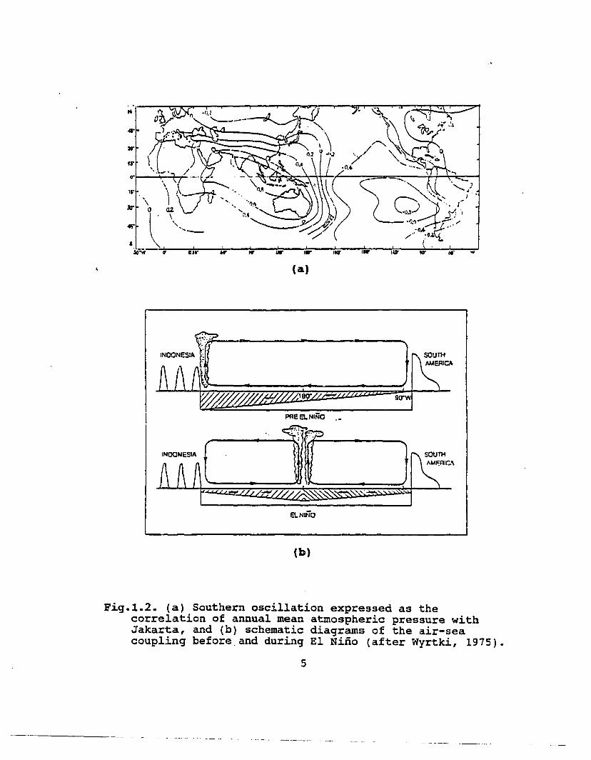
southeastern Pacific with alternating high or low pressure
fields over southern Asia (Fig.1.2). The interannual
variability of sea levels in response to ENSO may cause even
greater impacts on coastal erosion (see Komar and Enfield,
1987) than long-term trend of sea-level rise. For instance,
the 1982-83 El Nino raised the water level on the coast of
Oregon by 60 cm within 12 months, which changed the shape of
an inlet there due to erosion (Komar, 1986).
Atmospheric pressure and wind stress may be the major
factors for changes in water level on time scales of days to
months. In practice, the inverse barometeric response of
sea level to atmospheric pressure change is found to be a
significant part of seasonal changes in high latitudes
(Pattullo et al., 1955; Lisitzin, 1974).
An increase of atmospheric pressure by 1 mbar
(= 100 N m-2) causes the depression of the sea level
approximately by 1 cm. Tropical cyclones or hurricanes
result in peaks of mean sea level by the combination of
inverse barometric response and frictional processes. Since
hurricanes are maintained by the energy that they extract
from the heat in the ocean, thermal effects are very
important and the input energy is redistributed within the
ocean by stirring action of the storm in addition to
advective effects (Gill, 1982).
4
· .......3f'
t$'
0'
IF
1(1'\
0
4S" \ .
a \.Jo'w
(a)
lp~90"W
E\.NINO
(h)
Fig.l.2. (a) Southern oscillation expressed as thecorrelation of annual mean atmospheric pressure withJakarta, and (b) schematic diagrams of the air-seacoupling before,and during El Nino (after Wyrtki, 1975).
5
Isostatic land levels are changed by tectonic
activities such as volcanism, sea-floor spreading, faults
and subduction at the plate boundaries, glacial rebound,
sediment compaction, land subsidence, and hydroisostacy on
islands and continental margins. At active plate margins
such as the East Pacific Rise or Mid-Atlantic Ridge,
volcanic eruption from below the lithosphere, and the
transform faults, may change the volume or shape of the
local land masses. Due to the changes in spreading rate of
the sea floor or different spreading rates of the plates,
sea levels may be affected, although the effect is small
over time scales of less than a million years. At active
margins of the plates such as east of Japan and the
Philippines, two plates collide and the oceanic plate is
subducted beneath the continental plate, resulting in
earthquakes and vertical movements from deformation of the
land masses. Land tilting by different subsidence rates
between eastern and western sides of the Philippines is
shown in Fiq.I.3.
One of the most important factors in determining global
warming during the past century is the greenhouse effect:
increasing the surface air temperature by enhanced trapping
of longwaves radiated back from the earth's surface due to
greenhouse gases such as CO2 , CH4 , N20, and CFCs
(chlorofluorocarbons) in the atmosphere (Fig.l.4).
6

•. ,
20·r---r---------r-------A
15·
~
JOLO~.t7
o 200l<M, ,
TACLOB·1.5
~Zu.l
~
Fiq.l.3. Tilting of the Philippine Islands indicated byrelative land movement at 6 tide-gauge stations with2 mm/yr intervals. (-) represents land subsidence anddata are from PSMSL. (after Emery and Aubrey, 1991).
7

Since any body-material emits longwave radiation which is
proportional to the fourth power of the body temperature1,
both the earth's surface and the glass of a greenhouse (.or
the atmosphere) will be heated up until an equilibrium is
reached.
The most important factor causing the greenhouse effect
in the atmosphere is water vapor, of which the concentration
in the troposphere2 is determined internally within the
climate system and is not affected by human sources and
sinks on a global scale. The concentration of ozone (0 3 ) as
a second major greenhouse gas is changing in the atmosphere
due to human activities, but the lack of adequate
observations prevents us from accurately quantifying the
climatic effect of the changes in tropospheric ozone (IPCC,
1990).
There is little doubt that global MSL (mean sea level)
has risen by 10 to 30 cm during the past century. Some
local tide-gauge records nonetheless have deviated from the
global mean (from about 100 em rise in 20 years in Tribeni,
India, to about 160 cm fall in 14 years in Rorvik, Norway)
(see Appendix I in Emery and Aubrey, 1991).
1 Stefan-Boltzmann's law
2 the lowest atmospheric layer which is characterized bytemperature decrease from the ground (up to the height of200 mbar or about 10 km) and strong vertical mixing; theother three upper layers are stratosphere, mesosphere, andthermosphere from the lowest.
8

360 1800';' CARBO,. DIOXIDE '> ~ METHANEE i 1600Q. 340ez ~ 14000t= 320 t=<t oCIl: ~ 1200..2 30ew w1I ~ 100Gz0 0u 280 ·u... .. 800.0 xu u
260 6001750 1800 1850 1900 1950 2000 1750 1800 1850 1900 1950 2000
YEAR YEAR
3Ui 0.3'>';' NITROUS OXIDE
Zj I CFCll.a A-D. eCo
ID... zz ]::lC 0 0.20 t=t= oCc ~
rc ~..z W1Il U'': 2~0 . I z 0.1z 00 uu ..0 u...:: u,
2BO u0.0
1 ;"5 o 1800 1650 1900 1950 2000 1i'50 lBOO lil50 inoo l!hG ::0;)0
YEAR YEAH
Fig.l.4. Concentrations of greenhouse gases -- carbondioxide (C02 ) , methane (CH.), nitrous oxide (N20), andchlorofluorocarbons (CFCs) (after IPCC, 1990).

Due to uncertainties in the response of the atmosphere
and oceans to the greenhouse effect, several scenarios have
been suggested. Recently, the IPCC3 suggested that the
average rate of increase of global mean temperature and the
corresponding global MSL (mean sea level) rise are estimated
to be about 3°C (2°C to SOC) and about 60 cm, respectively,
before the end of the next century, under the 'Business-as
Usual Scenario' (Fig.I.S). There will be significant
regional deviations due to different contributing factors to
sea-level rise.
But the complexities of the feedback mechanism of
clouds regarding the increase of greenhouse gases in the
atmosphere, the oceanic response to the increase of
atmospheric temperature, and the interactions with snow and
sea-ice and with the biosphere still leave the uncertainty
range at least by about + 30 cm in recent predictions of
global mean sea level (see Wigley and Raper, 1992).
Four major climate-related contributing factors to
global MSL rise on a time-scale of 100 years are 1) thermal
expansion of the oceans, 2) glaciers and small ice caps, 3)
the Greenland ice sheet, and 4) the Antarctic ice sheet.
If the IPCC predictions are correct, sea-level rise
will accelerate over the next century. And the expansion of
3 Intergovernmental Panel on Climate Change, 1990
10

w 7en BUSINESS-ex: 6 AS-USUALwa: 5:::;)1--~(,)
4a:~WinQ"r,g
3::r--.w-1-1»
2>Q 0w.Qen ~ 1-..J<W 0a: 1850 1900 1950 2000 2050 2100
YEAR
-ECJ 120-w BUSINESS(J) 100 AS-USUAL-a:..J
80w>W-I 60-eUJenCu.sen 20-..J-eW 0a:
1980 2000 2020 2040 2060 2080 2100YEAR
Fig.l.S. (a) Simulation of the increase in global meantemperature from 1850 to 1990 due to observed increasesin greenhouse gases and predictions between 1990 and2100, and (b) the predicted sea-level rise showing thebest estimate and range, resulting from the Business-asUsual emmisions (after IPCC, 1990).
11
-------- ----

the tropics due to global warming may lead to an increase of
the frequency and intensity of tropical storms and
hurricanes (Wyrtki, 1990). Estimated contributions to sea
level rise over the past 100 years and for the near future
are shown in Table 1.1.
Table 1.1. Estimated contributions to sealevel rise duringthe past 100 years (upper) and between 1985 and 2030(lower) in em. Values in () are low and high estimatesbased on IPCC scenarios.
============================================================factors past 100 years 1985 - 2030
============================================================thermal expansion
mountain glaciers
Greenland ice
Antarctic ice
4 em(2 to 6 em)
4 em( 1.5 to 7 em)
2.5 em( 1 to 4 em)
o(- 5 to 5 em)
10.1 em(6.8 to 14.9 em)
7.0 em(2.3 to 10.3 em)
1.8 em(0.5 to 3.7 em)
- 0.6 em(- 0.8 to 0 em)
============================================================
Total10.5 em
(-0.5 to 22 em)(15 ± 5 em)"
18.3 em(8.7 to 28.9 em)
~===========================================================
* observed values of global MSL rise during the past 100years
There have been extensive efforts to reduce the range
of uncertainty in the prediction of future climate and sea-
12

level changes. Estimates by IPCC working groups (IPCC,
1990) are the most recent collaborative outputs, and hence
assumed to be the best predictions presently available.
Based on these estimates of global mean sea-level rise,
local rates of relative sea-level change in the Hawaiian
Islands, as well as in other selected North Pacific islands,
may be interpreted as to their possible causes.
The impact of short-term events such as hurricanes and
tropical storms are also significant on coastal erosion.
Storm waves are usually associated with wave set-up and
higher tides, and may erode part of the dunes. But it may
take fairly long (up to several years) to be recovered. The
erosional effect by storm waves could be enhanced by the
raised sea level; the beach erosion is maximized by the
storm waves at the maximum phase of sea level fluctuations
from daily to interannual time-scales.
But quantitative analysis of beach erosion due to storm
waves has been carried out mostly by model results, not by
measurements.
Shoreline changes due to cross-shore and longshore
sediment transport are a response of the coast to oceanic
forcing such as wind waves, tidal fluctuations, and storm
surges. Shoreline changes in this study will be examined
by:
13

1) historical aerial photographic analysis,
2) analysis of previous measurements of waves, and
sediment characteristics at Hawaiian beaches,
3) beach profile response models, based on the Bruun
Rule, for long-term trend and interannual oscillation
(Bruun, 1962; Dean and Maurmeyer, 1983) as well as for
short-term variation such as due to storm surges
(Kriebel and Dean, 1993),
4) cross-shore sediment transport rates and beach profile
changes on a few selected beaches with an energetics
based transport model by Bailard (1984),
5) beach recovery rates for model storm waves and sea
level fluctuation,
6) quantitative analysis of contributing factors to beach
erosion with different time scales,
From tide-gauge records and aerial photographs,
interannual trends of sea-level fluctuation and mean annual
oscillation superimposed on a linear long-term trend, from
monthly mean sea-level values, and the corresponding land
responses as shoreline changes are discussed in detail.
14
Time-series of daily MSL, winds and wave heights for
short-time scale fluctuations of sea level and land
responses are examined. Correlation between storms and
shoreline changes are also calculated before and after storm
events.
The Bruun Rule is applied to long-term trend,
interannual and annual sea-level fluctuations, due to its
simple relationship between sea-level rise and coastal
erosion. The concepts of equilibrium beach profiles (Bruun,
1954; Dean, 1977; Bodge, 1992; Pruszak, 1993), and closure
depths are discussed.
Short-term beach erosion was simulated by Bailard's
model (1984) at selected Hawaiian beaches. This model does.
not need any information about vertical profile of sediment
concentration in seawater but needs only near-bottom flow
velocity, which can be calculated from the input forcing
function (wave height and period). Therefore, it seems
attractive to use the energetics-based sediment transport
model (Bagnold, 1966; Bailard, 1984) when we want to know
the short-term relationship between input energy flux and
bottom profile change, although there are many assumptions
in the model. There has been no verification of the model
results by field measurements.
15

Based on the above measurements and computations, local
information regarding the rate of relative sea-level rise
and its impact on coastal erosion is described for Hawaiian
beaches. Calculation of cross-shore sediment transport
processes for selected Hawaiian beaches will further
illuminate the importance of characteristic time scales for
the erosive and regenerative developments.
16

CHAPTER 2
SEA-LEVEL RISE
IN TIlE HAWAIIAN ISLANDS
The Hawaiian Archipelago stretches about 1,500 miles
from west-northwest, Kure Island, to east-southeast, the
Island of Hawaii, which is the youngest island and still
growing. They have been formed by successive volcanic
activity, which is believed to be driven by the
northwestward drift of the Pacific lithospheric plate while
the hot spot in the
asthenosphere· stays fixed. Continual volcanic loading at
Kilauea, Hawaii, has made both the island itself and the
neighboring islands subside from isostatic adjustment.
Hence the subsidence rate is the largest at the Island of
Hawaii (+2.51 mm/yr at Hilo), second largest at the Island
of Maui (+1.04 mm/yr at Kahului), and relatively smaller at
the Islands of Oahu (+0.15 mm/yr at Honolulu) and Kauai
(+0.33 mm/yr at Nawiliwili), although these values are
subject to a large uncertainty.
4 one of the earth's interior layers classified by the platetectonic processes, which is at a depth range from about 100to 1,000 km in between lithosphere (upper rigid plate) andmesosphere (inner earth).
17

The total lengths of coastlines and beaches in the six
major Hawaiian Islands are as follows:
Table 2.1. The lengths (in miles) of the coastlines andthe beaches, and the ratio of beaches to coastline in themajor six Hawaiian Islands.
=======================================~~===================
island coastline total beaches . beach ratio=================================================m==========
Kauai 85 35
Oahu 129 50
Molokai 106 23
Lanai 52 18
Maui 159 31
Hawaii 306 19
41%
39%
22%
35%
19%
6%
==========================================================
Many drowned river valleys are found around the coasts
of Kauai. Oahu has more coastal plain and reefs and fewer
sea cliffs than the other islands. About half of the
coastline of Molokai is bedrock and sea cliff, and 25% of
the island is mud flat mangrove swamps, gravel, and
artificial structure. Most of the coastlines are composed
of bedrock -- about 70% (110 miles) in Maui and 90% (275
miles) in Hawaii (Walker, 1974).
18

Coral reefs grow in tropical waters where seawater
temperature exceeds about 18°C and water depth is limited to
less than a few tens of meters due to the need of sunlight.
Even in low latitudes, it is difficult for coral reefs to
grow along the west coasts of continents where upwelling is
prevailing and hence surface water is filled with subsurface
cold water lower than 18°C for part of the year. This is
because the earth's rotation effect (or Coriolis effect)
causes the wind-driven surface layer of the eastern boundary
currents (e.g., California Current, Peru Current in the
Pacific Ocean; Canary Current and Benguela Current in the
Atlantic Ocean) to move seawards and then subsurface cold
water rises to replace the surface water.
Corals are tolerant for a wide range of salinity
(30 PSll < S < 38 psu) unless there is a freshwater input
such as near an estuary where the salinity drops below 30
PSll (i.e., practical salinity unit). Some corals may grow
even in the Red Sea where the salinity is very high (S > 40
psu) (Guilcher, 1988).
While hermatypic corals construct the framework of the
reef, other organisms such as coralline algae, molluscs, and
crustaceans contribute to the reef fabric. Coral reefs are
highly productive ecosystems (in the order of 2,000 g-Carbon
m-2 yr-1) but energy demands are high, so that net production
19
is in fact quite low (about a few percent) (Carter, 1988).
The primary production is linked to the calcification
process of reef construction, and the food chains allow for
efficient recycling.
corals are rather minor contributors to the coral reef
communities in the Hawaiian Islands as a whole.
Foraminifera, mollusks, red (coralline) algae, and echinoids
(sea urchins) are more abundant. There are two common
mineral forms of calcium carbonate -- the fragments of the
skeletal parts of foraminifera and echinoids, and fragments
of red algae are found as the mineral calcite while those of
corals, mollusks, and green algae Halimeda are found as the
mineral aragonite.
Fringing reefs are the most common type of reefs in the
Hawaiian Islands. They are generally wide on the windward
and narrow on the leeward coasts of the islands of Kauai and
Oahu, respectively. Reefs fringing the west and north
shores are more irregular and deeper than the reefs on
windward or south shores, and have the well-sorted sandy
beaches with large annual changes (Noda, 1989).
A significant cause of relative sea level change and
sediment loss in the nearshore region of the Hawaiian
Islands results from the formation of beachrock, i.e.,
20
stratified calcarious sandstones or conglomerates common
along many tropical lime-sand beaches (Moberly et al.,
1963). Beachrock may form rapidly. As beachrock forms it
removes the sand, thus cemented, from the shoreline budget.
Once beach sands are transported to the offshore region,
some of the offshore sands are prevented from transporting
onshore by the reefs or trapped and cemented in the pores of
reef communities during the transport processes.
Meanwhile, reefs are protecting beaches from large
waves and are a source of sediments. Contrary to the
continental beach sands, Hawaiian beach sands are primarily
produced by some fishes eating, grinding, and puffing out
coral reefs (pers. comm., Krock, 1993). So the growth of
coral reefs also has substantial positive effects.
The effect of thermal expansion on sea-level rise in
the Hawaiian Islands is not expected to be large because of
small change in temperature and shallow depth of the mixed
layer in the tropical region, despite a relatively large
value of the thermal expansion coefficient which increases
from 0.8 x 10⁻³ at freezing temperatures to 3.4 x 10⁻³ at 30°C
(Wyrtki, 1990). Wyrtki estimates that the sea-level rise in
the tropics is only about one-tenth of that in polar
regions.
However, continuing long-term response to glacial
unloading causes global sea-level rise problems only at mid-
21
and low-latitudes because the land continues to rebound and
hence relative sea level sinks at high latitudes (Barnett,
1984; Lambeck and Nakibcglu, 1984; Emery and Aubrey, 1991).
Northeasterly trade winds are predominant over the
Hawaiian Islands, as much as about 86% of the year
(Fiq.2.1). The rest of the year is primarily affected by
southerly Kona winds. Short-term changes of beach systems
are basically governed by the wind waves. A local
atmospheric eddy over the lee side of the Island of Hawaii
due to trade winds (northeasterlies) may contribute to form
a? oceanic eddy. This orographic eddy may grow up to a
certain range (diameter > 100 km) and then start to drift
westward as Rossby waves with a speed of a few miles per day
(Patzert, 1969). The eddy forms a low (cyclonic) or a high
(anticyclonic) stand of sea level at its center, but it is
expected that the eddy may not significantly affect the
local coastal regions due' to its slow rotation.
In the Hawaiian Islands, the long-term rising trend of
relative sea level decreases from Hilo (+4.0 mm/yr), Hawaii
to the northwest islands (Fig.2.2). Continual volcanic
loading on Kilauea, Hawaii results in the subsidence of not
only the island Hawaii itself but also the neighboring
islands due to isostacy. The subsiding rate of the island
Oahu was estimated as about +1 to +2 mm/yr from the shallow
22

core measurements of a fringing reef crest at Hanauma Bay,
Oahu', (Nakiboglu et al., 1983), which is comparable to the
RSL rising rate of +1.6 mm/yr obtained from the tide-gauge
records at Honolulu Harbor, Oahu.
Yearl, ~n iCl6 '/.)
YOIOCr--r--r--r--r-....,~~---,.----r-....,.---,.---......c:<::I:0:
'"::-.....~.,
a<:) 75'It
oNosAJJMAMF
<:)
~ 5C':--~---:o:--~-~~._~_-I..--..I-_.J..._--'--_.r-._...J-_...JJ
Fig.2.1. Percentage of the trade winds (NE, E, and SE) forthe 5° squares between 15°N and 250N latitude at 150~ to1550W longitude plotted as monthly averages from ship'sobservations. Data from u.s. Navy Hydrographic Officepilot Charts (H.O. 560). (after Patzert, 1969).
23

~o. liawaii (1947-1988)2S
20 4.0 mm/yr ;
! I15 I:
10
5\' ,e I '
0 I . Ii~ I· :
-5
-10 .; I
-15
-20
-2S45 50 55 60 ·65 70 75 80 as 90
( a)
Kahului, Maui (1951-1988)
2.2 mm/yr
I I
I :
(b)
Fig.2.2. Long-term sea level trend (solid), 12-monthrunning mean (solid curve), and monthly sea level values
(dotted curve) at Ca) Hilo, Hawaii, (b) Kahului, Maui,(e) Honolulu, Oahu, (d) Nawiliwili, Kauai, (e) Johnston,(f) Midway, and (9) Mokuoloe, Oahu.
24

Honolulu, Oahu (1905-1988)2.5
20~ 1.6 nun/yr. I I I
15
10
S
B 0~
-s
-10
"-l ·ISVI
•2°1-
I .I I
, ,-2.50 5 10 IS 20 2.5 30 35 40 4S SO 5S . 60 6S 10 75 80 as 90
(c)
Fig.2.2. (continued) Long-term sea level trend (solid), l2-month running mean(solid curve), and monthly sea level values (dotted curve) at (a) Hilo,Hawaii, (b) Kahului, Maui, (c) Honolulu, Oahu, (d) Nawiliwili, Kauai,(e) Johnston, (f) Midway,' and (g) Mokuoloe, Oahu.

Nnwiliwili, Kauni (1955-1988)2S
20 L8 mm/yrIS ,I
, ;
10 ' ! I I;,
5
e 0.::!.
-5
-10
-IS
-20
-2545 50 55 60 6S 70 75 80 as 90
( d)
.,, .
. I
I "I " i: ,jI' ;' , I
. ,. ,I : u. I I, I, : I I I:
I, ' ii
; iSO 55 60 6S 70 75 80 as 90
( e)
Johnston (1950-1988)
0.4 mm/yr
II
I'll ! I! I '/'
II " : ,I ' I ,~:: I:'
I
25
20
IS
10
5
e 0~
-s-10
-IS
-20
-2545
Fig.2.2. (continued) Long-term sea level trend (solid),12-month running mean (solid curve), and monthly sealevel values (dotted cU~7e) at (a) Bilo, Bawaii,
(b) Kahului, Maui, (e) Honolulu, Oahu, (d) Nawiliwili,Kauai, (e) Johnston, (f) Midway, and (g) Mokuoloe, Oahu.
26

-0.6 mm/yr
Midway(1947-1988)
; I
90as8075706S60
Ii
55so
25
20
15
10
5
'8 0~
-5
-10
·15
-20
-2545
(f)
Mokuoloc:., Oahu (1957-74, 81. 1984-88)
A:,1 "'AI,:I!\~ ,,':~A • ('.
25
20
IS
10
5
'8 0~
·5
-10
·15
-20
-2545 so S5 60 6S 70 75 80
V"
as 90
(g)
Fig.2.2. (continued) Long-term sea level trend (solid),12-month running mean (solid curve), and monthly sealevel values (dotted curve) at (a) Hilo, Hawaii,
(b) Kahului, Maui, (c) Honolulu, Oahu, (d) Nawiliwili,Kauai, (e) Johnston, (f) Midway, and (g) Mokuoloe, Oahu.
27

At Midway Island station, the trend is even slightly
falling by about -0.4 mm/yr (Fig.6.3.(f»). This might be
related to the reef evolution in the Hawaiian Island chain,
running in a southeast and northwest direction. Scott and
Rotondo (1983) propose a general reef evolution model for
the Pacific plate; the 'moat and arch effect' acting at the
passage over an asthenospheric bump may result in a raised
atoll, which will sink later, leading to submerged atolls
and seamounts (Fig.6.4).
- .-ASTHENOSPHERE u~~
Fig.2.3. Proposed model for island development on thePacific plate. Arrows indicate subsidence (1) oremergence (T). HI: high island; FR: fringing reef;RBI-FR: raised high island with fringing reef;BR: barrier reef; AA: almost-atoll; A: atoll; RA: raisedatoll; SA: submerged atoll; G: guyot (simplified byGuilcher, 1988; originally from Scott and Rotondo, 1983)
28

The island of Maui subsides faster than the islands of
Oahu and Kauai, because it is closer to Hawaii and hence
more affected by isostatic subsidence due to volcanic
loading at Kilauea, Hawaii.
Hwang and Fletcher (1992) summarize the island
subsidence and the projected future submergence rates from
the tide-gauge records (Table 2.2).
Table 2.2. Sea level trends of rise in the HawaiianIslands. The numbers after ± represent standarddeviations. The unit is in em/decade (from Hwangand Fletcher, 1992).
============================================================station net subsidence future
submergence rate submergence------------------------------------------------------------Hilo 3.94 ± 0.23 2.51 + 0.53 8.51 + 4.09Kahului 2.46 + 0.23 1.04 + 0.53 7.04 + 4.09Honolulu 1.57 ± 0.08 0.15 ± 0.38 6.15 + 3.94Nawili- 1. 75 + 0.30 0.33 + 0.61 6.32 + 4.17wili
Their estimates of the linear trend from tide-gauge records
are a little higher than those analyzed in this study. They
assume that the subsidence rate of the islands is the net
submergence from the records minus the average (= 1.42 ±
0.30 em/decade) of the different estimates of global mean
29

-sea level rise (see Table 2, Hwang and Fletcher, 1992). The
corresponding island-specific subsidence rates then become
64% of the total submergence rate at Hilo, Hawaii, 42% at
Kahului, Maui, 10% at Honolulu, Oahu, and 19% at Nawiliwili,
Kauai, respectively. And the projected submergence rate is
assumed as the island-specific subsidence rate plus the
projected rate of future global sea-level rise, according to
the IPCC (Intergovernmental Panel on Climate Change) best
estimate scenario (= 6.0 ± 3.6 cm/decade) (IPCC, 1990).
If this is correct even when applying to the Hawaiian
Islands and linearly ~xtrapolated for the next. several
decades, the relative sea-level rise on the major Hawaiian
Islands is as follows (Table 2.3):
Table 2.3. Projected relative sea-level rise in 2040on the major four Hawaiian Islands~
============================================================island projected RSL rise in 2040
------------------------------------------------------------HawaiiMauiOahuKauai
42.6 + 20.5 cm35.2 ± 20.5 cm30.8 + 19.7 cm31.6 ± 20.9 cm
------------------------------------------------------------
30

Table 2.4. Mean monthly sea-level values and the standarddeviations of the annual cycles at the four major stationsin the Hawaiian Islands. Units are in cm, and the meanvalues are relative to the minimum values.
============================================================month
Jan
Feb
Mar
Apr
May
Jun
Jul
Aug
Sep
Oct
Nov
Dec
NawiliwiliKauai
4.9 ± 6.3
3.7 + 6.4
2.1 ± 5.8
1.1 ± 5.2
o + 5.0
0.7 + 5.4
4.7 + 6.4
8.5 + 6.7
10.7 + 5.5
9.8 + 5.0
7'.9 + 4.0
5.9 ± 4.8
HonoluluOahu
3.0 ± 6.8
2.4 ± 6.5
1.3 + 5.9
o ± 6.1
0.3 + 5.8
1.2 + 6.2
4.1 + 6.8
7.1 + 7.0
8.6 + 6.3
8.3 + 6.2
6.6 + 6.2
4.6 + 6.4
KahuluiMaui
4.1 + 5.6
3.2 + 4.7
1.8 + 4.3
0.3 + 4.5
o + 4.5
L8 + 6.0
5.2 ± 5.8
8.1 + 5.4
10.5 + 5.2
9.5 + 5.1
7.9 + 5.3
5.1 ± 5.0
HiloHawaii
4.3 + 7.6
2.2 + 6.9
1.8 + 7.1
0.9 + 6.2
o + 6.8
0.7 + 7.3
5.0 + 7.1
9.6 + 7.6
10.4 + 7.4
10.0 + 7.4
8.2 + 6.8
5.3 + 7.2
============================================================
31

Therefore, it is encouraged that the engineers
constructing coastal structures in the Hawaiian Islands
should adjust the design water level (DWL)5 due to sea
level rise at least by +50 to +60 cm, in addition to the
other effects, for the life-time of projects of 50 years.
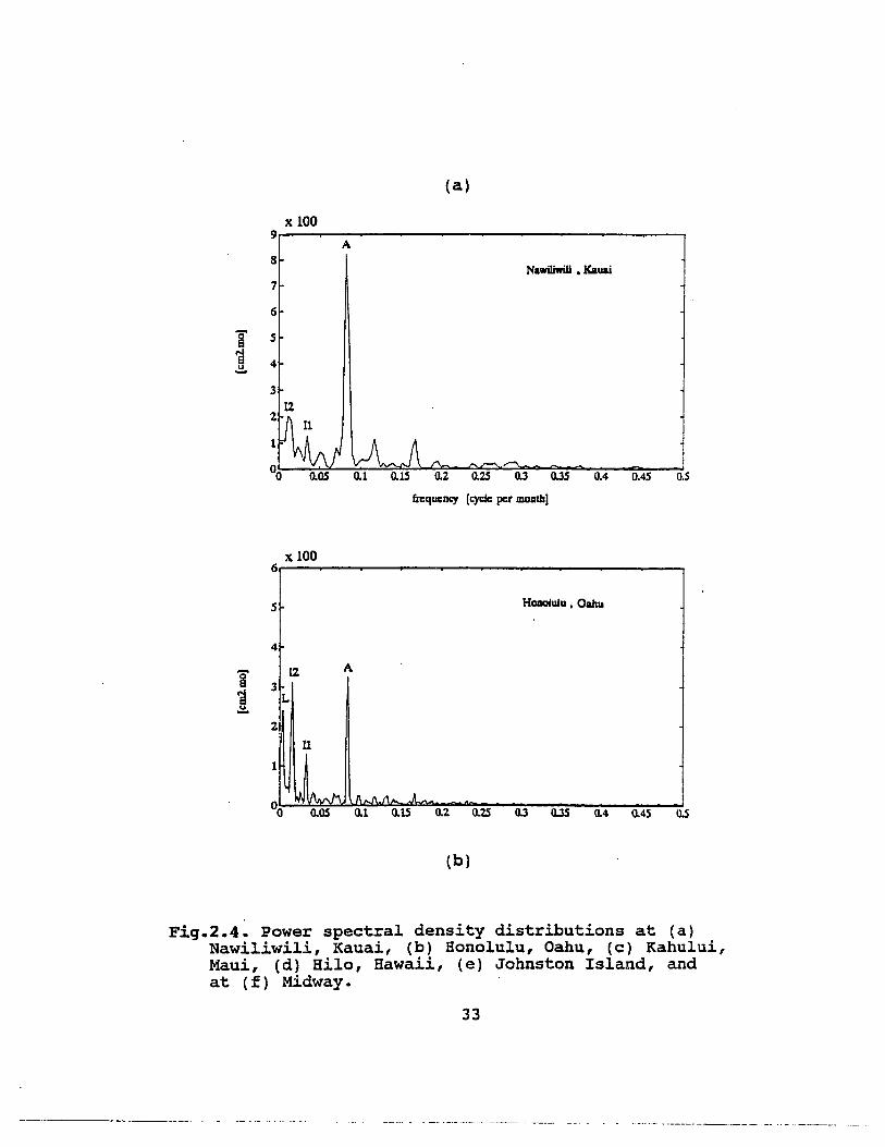
The fluctuation pattern of the monthly mean sea levels
in the Hawaiian Islands shows the annual and the interannual
oscillations. The interannual fluctuation shows typically
about 4-year period at Hilo (Hawaii), Honolulu (Oahu),
Kahului (Maui), Nawiliwili (Kauai) in the power spectral
density distribution (Fig.2.4). The mean annual cycle in
four major islands shows the difference of about 10 cm
between minimum (April to May) and maximum (September) sea
levels. The standard deviations of the mean annual cycle
range from 4.0 to 7.6 cm (Table 2.4).
5 OWL = MLLW + AsT + InB + wis + Was + WaR + LoT· + IaF"·MLLW Mean Lower Low WaterAsT Astronomical TideInB Inverse Barometric Effectwis Wind setup (storm surge or piling-up by coriolis effect)WaS Wave setupWaR Wave Runup (It is usually not included in OWL, but added
later, if appropriate.)LoT" : Long-term TrendIaF"·: Interannual Fluctuation
(The last two terms in the righthand side are suggested by the author.)
32
(a)
x 1009
A8
7
6
i 5
'i 4~
Nlwi1iwiIi • Kauai
0.25 o.J o.J5 0.4 0.45 0.5
frequency (cycle pet lIIOatbJ
X 1006
S~ Honolulu, Oahu
4
i 12. A
3'i L~
2
U
1
\.AIlkM II n" .A.°0 0.05 0.1 0.15 0.2 0.25 o.J o.JS 0.4 0.45 us
(b)
Fiq.2.4. Power spectral density distributions at (a)Nawiliwili, Kauai, (b) Honolulu, Oahu, (c) Kahului,Maui, (d) Hilo, Hawaii, (e) Johnston Island, andat (f) Midway.
33

(c)
x 100
A
Maui
0'8
1
o O.OS 0.25 0.3 0.35 0.4 0.45 0.5
fn:qucncy [cydc per month)
x 1007.--.....--......--....----.......- .......--..-----.....--~
A
6
5
Hila Ha-u
( d)
0.35 0.4 0.45 as
Fig.2.4. (continued) Power spectral density distributionsat (a) Nawiliwili, Kauai, (b) Honolulu, Oahu, (c)Kahului, Maui, (d) Hilo, Hawaii, (e) Johnston Island,and at (f) Midway.
34

(e)
x 10018
A
16 JolmatoD
14
12
'0108
N8~ 8
o D.3S 0.4 0.45 usfrequency [cyda par month)
x 1007,.----_-_--_-_-......- __-_-__.....A
'08
1
o 0.05
(f)
0.4
Fig.2.4. (continued) Power spectral density distributionsat (a) Nawiliwili, Kauai, (b) Honolulu, Oahu, (c)Kahului, Maui, (d) Hilo, Hawaii, (e) Johnston Island,and at (f) Midway.
35

CHAPTER 3
METHODS .AHD ANALYSES
3.1. AVAILABLE DATA
3.1.1. Tide-gauge Records
Two sources of sea· level data -- PSMSL (Permanent
Service for Mean Sea Level6)and TOGA (Tropical Ocean and
Global Atmosphere7 ) program -- are used. Fourteen island
stations in the North Pacific between the equator and 35°N
are selected for monthly sea level values from PSMSL, among
which seven stations in the Hawaiian Islands are chosen both
from PSMSL (monthly means) and TOGA (daily means). The
locations and the durations of the data are shown in Table
3.1.
TOGA daily data at the 7 stations in the Hawaiian
Islands are calculated using a two-step filtering operation.
First, the dominant diurnal and semidiurnal tidal components
are removed from the quality-controlled hourly values.
Secondly, a 119-point convolution filter (Broomfield, 1976)
6 Bidston Observatory, Birkenhead, Merseyside, L43 7RA, U.K.
7 TOGA Sea Level center, university of Hawaii, 1000 Pope Road,Honolulu, HI 96822, U.S.A.
36

Table 3.1. The locations and the lengths of the PSMSL(monthly MSL) and TOGA (daily MSL) data at theselected island stations in the North Pacificbetween the equator and 30~.
============================================================station latitude longitude period years
40(18)40(18)82(18)30(10)32(18)
(15)
40(17)37(18)37
22
41
40
41
42
41
1947-86(1973-90)1947-86(1973-90)1905-86(1973-90)1957-86(1981-90)1955-86(1973-90)
(1975-89)
1947-86(1974-90)1950-86(1973-90)1950-86
1951-72
1946-86
1947-86
1948-88
1947-88
1948-88
157°47 'w(157°48 'W)159°21 'w
13°09 'N
20°45 'N(20°54 'N)21°19 'N
(21°18'N)21°26 'N
Island
Island
Philippines
Kwajalein Island
Eniwetok Island
Honolulu, Oahu
Wake Island
Hilo, Hawaii
Mokuoloe, Oahu
Legaspi, Philippines
Kahului, Maui
Nawiliwili, Kauai
Guam
Davao,
Truk
French Frigate Shoal
Midway Island
Johnston Island
-----------------------------------------------------------Valuee in () 8Ze for the location. or duration of TOGA data, when different from PSMSL data, in theaawaiian Ialanda.
37
--_ ..._-----_._---

centered on noon is applied to remove the remaining high
frequency energy and to prevent aliasing when the data are
computed to daily mean values (Caldwell et al., 1989).
TOGA monthly data are calculated by simply averaging
all the daily mean values in a month. If a missing period
is longer than seven days in a month, the monthly values are
not calculated and but substituted either by linear
interpolation or by weight-folding method (WFM) within a
time-series (see section 3.2).
Historically, sea level has been simply measured by
reading the relative height of water level to a convenient
bench-mark, e.g., a vertically mounted scale on a pier or
wharf etc. There are a few different types of tide-gauge;
float-type with a stilling well, bubbler-type with an air
tank, and pressure sensor.
Typical pressure-sensor and field accuracies are
reported as ±2 cm and ±5 cm, respectively (Rayner and
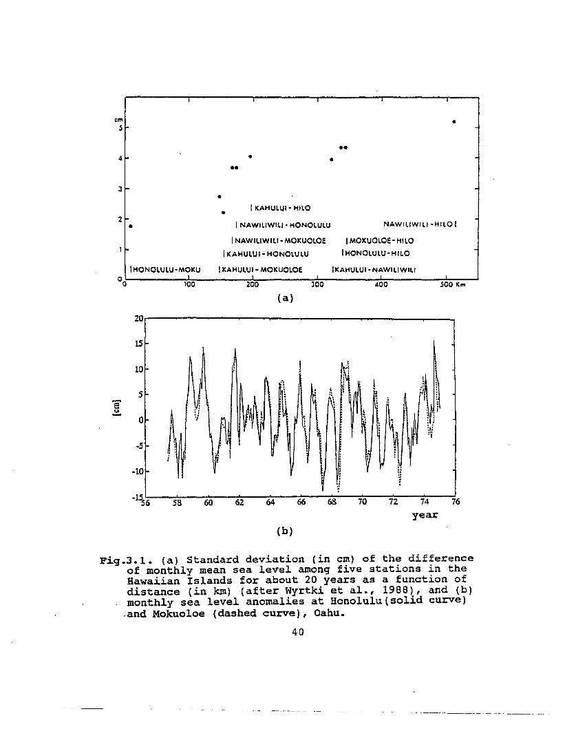
Archer, 1985). Wyrtki et al. (1988) estimate monthly mean
sea level values as representative with an accuracy of ±2 em
from calculating the standard deviations of monthly mean sea
level between pairs of stations at 5 stations in the
Hawaiian Islands for about 20 years (Fig.3.1.(a)). Time
series of monthly sea level anomalies between Honolulu and
Mokuoloe during 1957 to 1975 shows almost no phase lag with
38
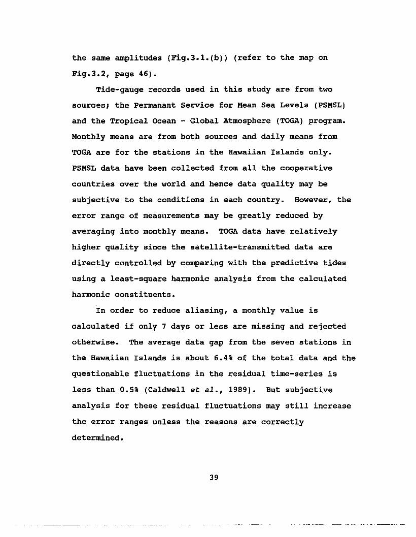
the same amplitudes (Fig.3.1.(b» (refer to the map on
Fig.3.2, page 46).
Tide-gauge records used in this study are from two
sources; the Permanant Service for Mean Sea Levels (PSMSL)
and the Tropical Ocean - Global Atmosphere (TOGA) program.
Monthly means are from both sources and daily means from
TOGA are for the stations in the Hawaiian Islands only.
PSMSL data have been collected from all the cooperative
countries over the world and hence data quality may be
subjective to the conditions in each country. However, the
error range of measurements may be greatly reduced by
averaging into monthly means. TOGA data have relatively
higher quality since the satellite-transmitted data are
directly controlled by comparing with the predictive tides
using a least-square harmonic analysis from the calculated
harmonic constituents.
In order to reduce aliasing, a monthly value is
calculated if only 7 days or less are missing and rejected
otherwise. The average data gap from the seven stations in
the Hawaiian Islands is about 6.4% of the total data and the
questionable fluctuations in the residual time-series is
less than 0.5% (Caldwell et al., 1989). But subjective
analysis for these residual fluctuations may still increase
the error ranges unless the reasons are correctly
determined.
39
em51-
I
•
4
•
••• •
••
•2
•
I KAHULUI- t"1Il0
I NAWILIWILI- HONOLULU
INAW1LlWILI- MOKUOLOE
I KAHULUI- HONOLULU
NAWILIWlll -HILO I
IMOKUOLOE- HILO
IHONOLULU-HILO
IHONOLULU' MOKU
00 100
1KAHULUI- MOKUOLOE IKAHULUI- NAWILIWILI
200 300 400
( a)
SOO Km
20
15
10
58"~
0
-5
-10
-1556
i .
58 60 62 64
(b)
66
···J
68 70 72 74 76
year
Fig.3.1. (a) Standard deviation (in cm) of the differenceof monthly mean sea level among five stations in theHawaiian Islands for about 20 years as a function ofdistance (in km)(after Wyrtki et al., 1988), and (b)monthly sea level anomalies at Honolulu (solid curve)
.and Mokuoloe (dashed curve), Oahu.
40

For the purpose of this study, data gaps are filled
either linearly or by using WFM (Weight-Folding Method) as
described in the next section (Section 3.2). Although WFM
is based on the assumption that the nearer (missing) datum
may have a higher correlation than the farther one, which
seems to be more reasonable than the linear interpolation,
this must not be always true and may be more biased than the
linear interpolation in some cases. However, one obvious
intention of this method is to create a continuous time
series not biased from the real time-series with a fortnight
(= 14 days) tidal component in daily values and with an
annual component in monthly values, respectively.
3.1.2. Aerial Photographs
Pre-analyzed aerial photographs on Oahu (Hwang, 1981)
and on Maui, Kauai, and Hawaii (Makai Ocean Engineering,
Inc., 1991) are primarily used to examine beach erosion and
shoreline changes in the Hawaiian Islands. The time
difference between first and last photos at each site is
approximately from 25 to 40 years (3 to 5 photos with about
a 10 year interval). The average numbers of transects at
each site are as follows: 4 to 7 transects on Oahu, 3 to 5
on Kauai, 3 on Maui, 4 on Molokai, 2 to 3 on Hawaii. They
were measured by the deviations of vegetation line and water
41

line from those in the base year (i.e., cross-shore beach
distance between water line and vegetation line), using the
method of photogrammetry. The locations and number of data
selected from the previous analyses are as follows (Table
3.2) :
Table 3.2. The location and the number of transects (ornumber of sites) of the aerial photographs in the fourmajor Hawaiian Islands. Data selected (or averaged)from Makai Ocean Eng.(1991) and Hwang (1981).
============================================================island location no. of no. of period
photographs transects------------------------------------------------------------
KA (southwest) 4 11 1953-88KB (southeast) 4 9 1953-88
Kauai KC (east) 3 - 4 36 1950-88KD (northeast) 3 13 1960-88KE (north) 4 10 1950-88KF (north) 3 - 4 6 1950-88
Oahu north 3 - 7 82 (12) 1928-79windward 4 - 7 133 (14) 1928-80south 3 - 6 52 (11) 1928-79leeward 4 - 6 41 (10) 1949-79
------------------------------------------------------------Maui MA (west) 3 - 4 25 1949-88
MB (southwest) 4 19 1949-88MC (southwest) 4 - 5 23 1949-88MD (north) 4 21 1950-88
------------------------------------------------------------Hawaii HA (northwest) 4 11 1950-88
HB (west) 4 - 6 18 1950-88
42

Shoreline changes from aerial photographs, based on the
previous analyses by Makai Ocean Engineering and Sea
Engineering (1991) and Hwang (1981), were carefully re
analyzed, including an annual oscillation of sea level with
the average slope of beach profile.
The traditional way of interpreting aerial photographs
for long-term change of shoreline is to determine vegetation
line or water line by eye, which involves some level of
subjectivity and inconsistency in the detection process
since the coastline as a transition zone between land and
sea forms a complex system of ~rightness variation in the
panchromatic spectrum (Shoshany and Degani, 1992).
In general, errors come from two typical sources; those
are
1) errors due to photographic processes such as lens
distortion, camera tilt, film development, differential
scale change from the center to the margins, and relief
displacement, etc., and
2) errors due to geometrical adjustment between
photographs and base map.
Relief displacement changes radially from the center of
the photo, which is coincident with the nadir point (the
43

point vertically below the camera) for a truly vertical
photo. Since most coastal features have low relief, radial
distortion due to elevation differences is not serious.
Lens distortion and camera tilt may result when an
airplane and camera are not exactly parallel to the mean
plane of the earth's surface at the instant of exposure.
About half of near-vertical air photos taken for domestic
mapping purposes are tilted less than 2 degrees, and few are
tilted more than 3 degrees (Wong, 1980).
Scale change may result from the shifts in altitude
along the photographic flight line, especially with light
aircraft. The possible decrease of the aircraft elevation
may significantly increase the scale of the air photos.
An interesting example of the error by changing scale was
reported by Anders and Byrnes (1991):
If an air photo were used to measure a shoreline
distance by 10 em for an assumed scale of 1:20,000, ground
distance would be calculated at 2,000 m. However, if the
actual scale were 19,934 m resulting from the decrease of
the aircraft elevation by 10 m at the moment of camera
exposure, which is common iri small light planes, then the
distance would be 1,993.4 m. This produces 6.6 m difference
in location of the shoreline point.
44

Thus exact scale should be determined for digitizing
data from each air photo. Photographic scale (0) is
calculated by
where
fQ ,. '"
(3.1)
f = focal length of the camera lens
( = flight altitude of the camera above the mean
elevation of the terrain
Correct interpretation of the HWL (high water line)
and careful annotation are required to avoid large
miscalculations. For a 1:20,000 scale, a 0.2 mm line drawn
with a very thin drafting pen makes a ground line with 4
meter width. Therefore, in order to minimize error
associate with shoreline annotation, photographic scale 0
should be maximized, that is, measurement altitude must be
low and camera lens should be large.
Displacement of an image due to radial distortion
resulting from elevation changes (De) can be calculated as,
De ,.
45
rhT (3.2)

where
r = distance from the center of the image to the top
of the object,
h = ground elevation of the object,
= flight altutude of the camera
Lastly, displacement of a point on an aerial photograph
due to tilt (De) from its actual ground position can be
calculated by
r 2 sinal: cos28
f - r sinOecos8
where
r - distance from the point to the isocenter,
f = focal length of the lens,
at = angle of tilt of the photograph,
(3.3)
e = angle from the principal line to the radial line
(clockwise) between isocenter and the point
within the plane of the photograph
46

3.1.3. Waves
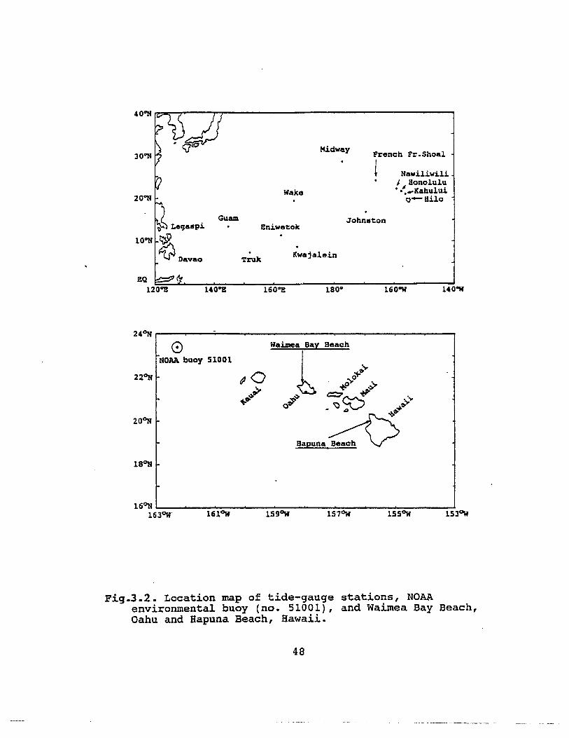
Twelve-year wave data from NODCs (January 1981
August 1992) are to be used, which had been measured by
NOAA9 environmental buoy (no. 51001) at the northwest of
Kauai (23°24'N, 162°18'W) (Fig.3.2).
Significant wave heights were corrected for low
frequency noise, and wind speeds and directions with the
original 8.5 minute interval were averaged for an hourly
interval by TOGA Sea Level Center, University of Hawaii
(pers. comm., Caldwell, 1993).
Maximum estimates of visual surf observations at five
locations (Sunset Beach, Makaha, Ala Moana, Diamond Head,
and North Beach) on Oahu during 1988 to 1992 are also used
for examining the correlation between deep-water wave
heights and surf heights. Since the data sources are the
radio, National Weather Services, and personal observations,
they are subjective to the observers.
S National OCeanographic Data Center
9 National Oceanic and Atmospheric Administration
47
140"W160"W
French Fr.ShoalI
l NawiliwiliI Honolulu••~ ..Kahului
·,,-ailo
John.ton
Kidway
Kwajalein
Wake
160"2
EniwetOk
1!ruk
30"N
40"N I?'::"'~~--r-r-------------------"'"
20"N
24or. r---.......----:;---.---------.------.-----.
oNOAA buoy 51001
lSSOWlS70WlS90W1610W16or. l- ~~-""--.......=__---'-------""'-----.....J,
1630W lS30W
Fig.3.2. Location map of tide-gauge stations, NOAAenvironmental buoy (no. 51001), and Waimea Bay Beach,Oahu and Bapuna Beach, Hawaii.
48

The basic problem in measuring waves is that of
sampling a time-varying process which is spread out on a
two-dimensional surface. Buoys have been typically used for
measuring waves. So the quality of the measurements has
been dependent on the buoy's ability to follow the sea
surface faithfully. A directional buoy is often used in
recent days, which provides the information of wave
approaching directions and allows us to decompose wave
energy with respect to both frequency and angle. However,
the mooring line may still give a significant effect on buoy
motion.
NOAA environmental buoy (no.51001) moored at a location
northwest of Kauai (23°24'N, 162°18'W) is an accelerometer
type wave measuring device, which obtains vertical
displacement information of the buoy by electrically
integrating vertical acceleration twice.
The total observational error may include several
components as follows:
1) static instrument measurement error ••• residual error
after calibration
2) dynamic measurement error ••• error from the induced
motion of the sensor due to buoy motion, the effect of
49

the dynamic response or instability of the instrument to
environmental changes
3) physical disturbance error ••• error due to the
superstructure or subsurface data line of the buoy
4) data manipulation and processing error ••• data
distortion in transferring, storing, retrieving or
digitizing
5) transform error ••• effect due to averaging or converting
the environmental parameter
6) dislocation error ••• error from temporal and spatial
dislocations of the sensor due to response time,
currents" weather, imprecise navigation etc.
Folkert and Woodle (1973) reported the representative
error estimate of wave height from the accelerometer-type
wave-rider buoy as 0.39 m, which includes the error
contributions from transducer (= 0.2 m), signal conditioning
(= 0.22 m),' calibration (= 0.22 m), platform motion (= 0.13
m) •
Other authors presented the estimate of error as ±15 cm
in 5 m (or ±3 %) by typical instrument sensor and ±20 cm in
field accuracies, for this type of wave sensor (Rayner and
Archer, 1985).
50
The calibration of wave-height sensing systems, e.g.,
the accelerometer transducer which is one of the most
significant and principal error sources, is difficult but
must be very precise since the measurement of wave height
involves the double integration of low frequencies. But
the more significant problem in performing adequate
calibration is the lack of a true measure of the sea surface
elevation. Apart from the problems with sensor calibration,
the suspension platform of the buoy may be set into
oscillation causing a low frequency drift in the signal
(Fig.3.3).
Averaging wave heights and periods into hourly values,
which was done by TOGA Sea Level Center, University of
Hawaii, smooths the measured time-series from the wave buoy
to a great degree. And daily mean values for obtaining the
wave climate in this study will be even much smoother than
the measured time-series, which will completely remove high
frequency peaks.
51

!te:.
~ ~r'N4t~lW~JI~lI~L""i ~ ,~ ,~ 2~
·"~~l ..n~..-~;;;~. ,;0;"
see,
~~~~~ S~ .'.0 7~. 7:'-
~ H/~ ~~VYWlY'4(MW~,NifN\~~I ~
(a)
Fig.3.3. (a) Example of a time series with low frequencydrift and (b) the spectrum of the record. This serieswas recorded with a Hippy 120 sensor (~o ~ 2n/120s).In this case the spectra will be correspondinglycompressed towards 0 Hz. (after Barstow et al., 1985)
52
------------- - -----
3.1.4. Beach Profiles and Sediment Characterisitics
Measured beach profiles, sediment characteristics such
as sand size, seasonal change of the size (Moberly and
Chamberlain, 1964; Gerritsen, 1978; Parker, 1987) and sand
volumes and widths of beach reservoirs (Chamberlain, 1968)
in the past are also important data to be calculated with
cross-shore sediment transport models, and compared with
other data such as aerial photographs, as mentioned above.
53

3.2. METHODS
3.2.1. Mean Sea Levels
3.2.1.1. Filling Gaps in MSL Data
Data gaps are treated by three different ways:
1) gaps shorter than 6 months in monthly mean values (or 7
days in daily mean values) are linearly interpolated.
2) gaps equal or longer than 18 months in monthly mean values
(or 21 days in daily mean values) are left as they are.
3) gaps in between 1) and 2), that is, equal or longer than 6
months but shoter than 18 months in monthly mean values (or
equal or longer than 7 days but shorter than 21 days in
daily mean values) are interpolated by the Weight-Folding
Method (WFM).
WFM is carried out by three steps: take the same lengths
of the neighboring data as that of a gap from both sides, and
fold the neighboring data into the gap from endpoints (Bo and
Ao ) . Then, subtract these data values from the doubles of the
data at endpoints (2B o - B1 and 2Ao - AL_1 ) . Lastly, multiply
linearly different weighting factors from both ends to the
above values and add up the two resultant values to create a
gap datum (Fig.3.4). This can be expressed as the following
simple relationship such that
54

(3.4)
where Bot A o ::I endpoints before and after the gap
Bi = i-th data backward before the gap
AI.-J. ::I (L-i)-th data after the gap
Ci ::I created data for the gap by WFM
L ::I the length of the gap
25.-------....----.......---....---__-----,
'8...-
·20
0- real data
• - created data
195419531952·1f9~51---"'---~';::---"""'----:-==-----'-----:-::·
Fig.3.4~ Example of Weight-Folding Method for a caseof monthly time-series with a gap of 11 months.Dotted line between Bo and Aa is a linear interpolation,and Ci's are created data from Bot Bi's and Aa, AJ.'swith linearly interpolating weights.
55

3.2.1.2. Linear Regression
The whole time-series of data at each sea-level station
is linearly fitted by the least squares method in order to
determine the long-term linear trend. When the data gaps are
too large and hence not filled, each data segment is linearly
fitted, independently, such as at Mokuoloe, Oahu. Even for a
continuous time series, rising or falling trends in an
interannual scale by parts are selectively analyzed by linear
regression.
3.2.1.3. Averaging and Smoothing
In order to obtain the mean annual cycle at each station,
all the data in each month during the whole period are simply
averaged after they are detrended, i. e ., the mean and the
linear long-term trend are removed. For analyzing interannual
fluctuations, smoothing with twelve-month-running-means is
applied. Hanning's filter (a bell-shaped window) is also used
for obtaining the power spectral distribution of a time
series. This smoothing filter' is applied before the time
series is transformed by Fast Fourier Transform (FFT).
56
3.2.1.4. Spectral Analyses
It is difficult to identify the frequency components from
looking at the original signal. Fourier transform (or Fourier
integral) of any signal in a time-series gives the
distribution of signal strength with frequency.
Fast Fourier Transform (FFT) is applied to get a power
spectral density distribution of monthly sea level values
after they are smoothed by Hanning's filter with the width of
12 months. FFT is substantially faster in computer analysis
than direct Fourier transform and hence popularly used now for
a time-series of any power of two. If the length of a time
series is not an exact power of two, it is padded with
trailing zeroes.
57

3.2.2. Models
Models for long-term trend and interannual variation of
beach profiles are basically governed by the relative sea
level changes while the short-term response models are
controlled by waves.
Beach profile response model by Bruun (1962) is applied
to long-term trends (> 20 years) and to several-year-period
fluctuations of sea level and beach profile changes. Based on
observed long-term sea-level rise and interannual
oscillations, the relationship between shoreline retreat and
beach erosion will be examined.
Equilibrium profiles suggested by Dean (1977) and Bodge
(1992) are also discussed, as well as Pruszak (1993) who
introduces a time-dependent parameter for Dean's function (see
next section in this chapter). Short-term response models by
Edelman (1968), by Kriebel and Dean (1993), and by Steetzel
(1990) are to be reviewed, despite the response time to
establish an equilibrium profile.
An energetics-based model by Bailard (1984) is used to
simulate beach profiles at Waimea Bay, Oahu and at Hapuna
Beach, Hawaii for different wave heights in a time-scale of a
few months. This model is represented by the beach profile
changes and cross-shore sediment transport rates with one-week
intervals.
58

3.3. ANALYSES OF SEA-LEVEL CBABGBS
Major reasons of the long-term trend of relative sea
level height are thermal expansion of ocean surface waters,
changes in the Greenland and Antarctic ice sheets, and the
melting of mountain glaciers (Gornitz and Lebedeff, 1987;
Barnett, 1988; Peltier and Tushingham, 1989; Trupin and Wahr,
1990; Douglas, 1991). In addition to the eustatic sea level
rise due to global warming and glacial melting as mentioned
above, there are other factors; land fall/rise or tilting due
to local tectonism such as volcanic activity, sea floor
spreading, subduction of a plate into another plate at the
plate boundary, volume change in ocean basin due to the above
tectonic effect, land transformation due to long-term sediment
transport, coral reef formation/growth and so on.
Annual oscillation and interannual fluctuation as well as
long-term trend of relative sea levels would contribute
altogether to coastal erosion. Although some author, e.g.,
Pruszak (1993), includes another signal of the sea-level
fluctuation with a period of 20 to 30 years, it is excluded in
this study because of data lengths. Long-term linear trend is
considered with the Bruun Rule; a simple geometric conversion
of shoreline retreat from sea-level rise and beach-slope with
some restrictions in the sediment transport processes. Annual
oscillation and interannual fluctuation are analyzed to deduce
59
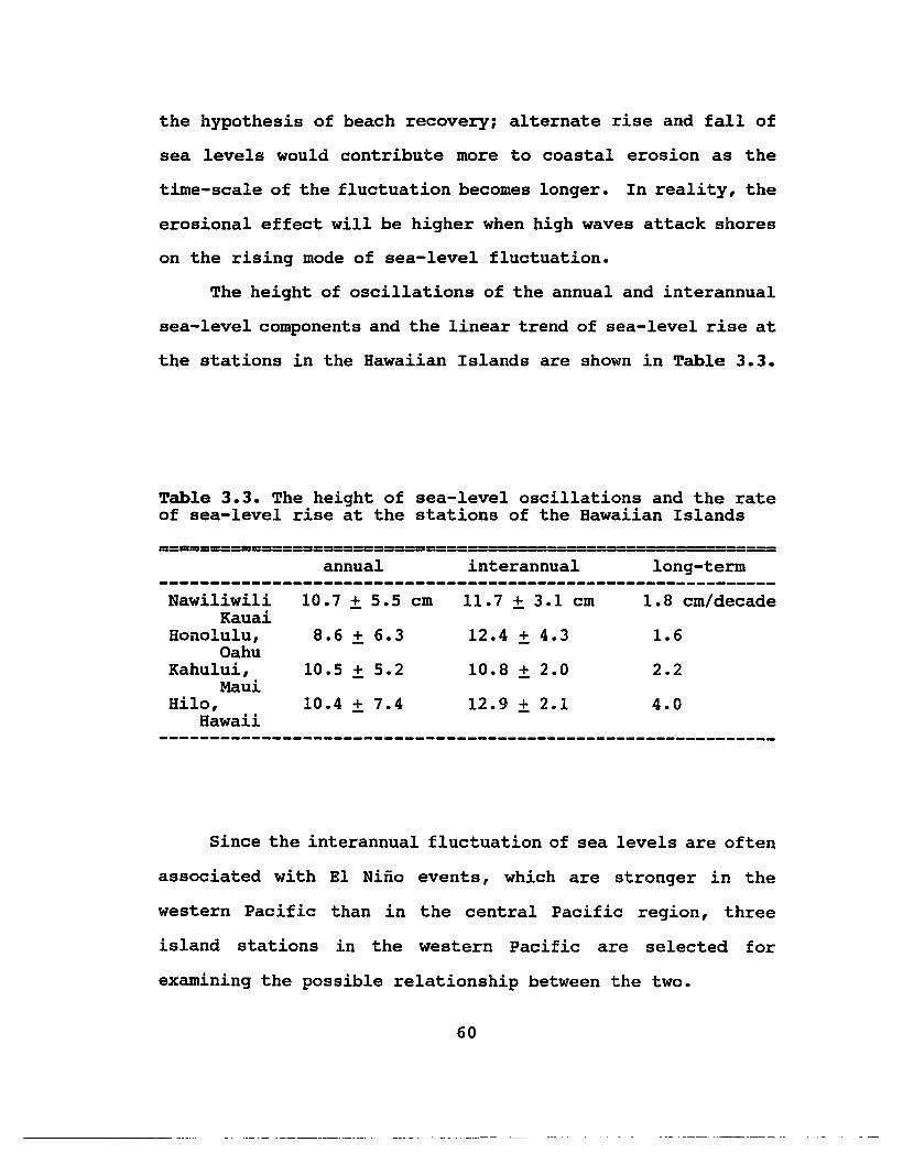
the hypothesis of beach recovery; alternate rise and fall of
sea levels would contribute more to coastal erosion as the
time-scale of the fluctuation becomes longer. In reality, the
erosional effect will be higher when high waves attack shores
on the rising mode of sea-level fluctuation.
The height of oscillations of the annual and interannual
sea-level components and the linear trend of sea-level rise at
the stations in the Hawaiian Islands are shown in Table 3.3.
Table 3.3. The height of sea-level oscillations and the rateof sea-level rise at the stations of the Hawaiian Islands
======================== ----annual interannual long-term
Nawiliwili 10.7 ± 5.5 em 11.7 ± 3.1 em 1.8 em/decadeKauai
Honolulu, 8.6 + 6.3 12.4 + 4.3 1.6Oahu
Kahului, 10.5 + 5.2 10.8 + 2.0 2.2Maui
Hilo, 10.4 ± 7.4 12.9 + 2.1 4.0Hawaii
-------------------------------------------------------------
Since the interannual fluctuation of sea levels are often
associated with EI Nino events, which are stronger in the
western Pacific than in the central Pacific region, three
island stations in the western Pacific are selected for
examining the possible relationship between the two.
60
~--- ~-- ---

•
At the 3 western Pacific island stations, Truk, Wake, and
Kwajalein, the long-term linear trend varies at about +1 to +2
mm/yr (Fig.3.S). But the fluctuations of the averaged time
series data smoothed by 12 month running mean show quasi
periodic oscillations with several-year period, which
correspond to the peaks of a low-frequency signal larger than
the annual signal in the power spectral distribution
(Fig. 3.7) • They seem to respond to the historic El Nino
events with certain time lags, according to the time-series of
the monthly mean sea-level heights.
At Truk Island, the two peaks with the periods of about
2 to 3 years are larger than the annual peak, and the semi
annual and 7-year signals are slightly less than the annual
signal •
At Kwajalein, the 7-year signal is predominant and an
annual signal is not clearly shown in the power spectra. In
other words, the signals with semiannual, 10 months, annual,
and biannual periods are comparable but much smaller than the
peak with the 7-year period. At Wake Island, there exist many
spectral peaks, which makes it difficult to analyze the
mechanism of the sea level changes. A 10 to 11 year peak and
an annual signal are comparably dominant, and there are
several other smaller peaks with the periods from 5 years to
3 months.
61

Truk IsL(1950-1988)2S
20 1.7 mm/yr15 i. "
10
5 ' !I
e 0~
-5
-2545 50 55 60 65 70 75 80 as 90
( a)
2SKwajaJcin IsL(1946-1988)
20 1.1 mm/yr15 ,.10
5
e 0~
I'
-s·10
-15
-20
-254S 50 55 60 65 70 75 80 90
(b)
Fig.3.5. Long-term sea level trend (solid line), 12-monthrunning mean (solid curve), and monthly sea level values(dotted curve) at (a) Truk, (b) Kwajalein, and (c) WakeIslands in the'wetern Pacific Ocean.
62

25Wake IsL(1950.1988)
! !20 2.1 mm/yr15 !I
,I I I
,10 ! i5 I
a 0~
·5
(c)
Fig.3.5. (continued) Long-term sea level trend (solid line),12-month running mean (solid curve), and monthly sealevel values (dotted curve) at (a) Truk, (b) Kwajalein,and (c) Wake Islands in the wetern Pacific Ocean.
63
The mean annual difference of sea level height at the
island stations of the western Pacific is about 10 cm, as is
seen in the Hawaiian Islands. The maximum and minimum levels
at Truk Island (about 7.5~, 152~) and Kwajalein (about 9~,
168°E) occur in April and in January, respectively
(Fig.3.6. (a), (b)). Surprisingly, at Kwajalein the monthly
mean sea level height is almost flat (approximately 2 cm below
the maximum level) from June to October after the maximum in
April.
The annual pattern of the monthly mean sea level height
is drastically different at Wake Island (about 19~, 166.5~),
which shows a maximum in August and a minimum in May
(Fig.3.6.(c)). There exists a slight secondary peak (about 3
cm higher than minimum level) between April and June. The
secondary peak at Truk and the maximum level at Wake occur in
the same month, October.
At Guam (about 13~, 144~) and at Eniwetok (about 11~,
162~), the patterns of the mean annual cycle are nearly
sinusoidal and have almost the same phase as the sun's
altitude, that is, maximum in june to July and minimum in
December (Fig.3.6.(d),(e)). But the reason for this
coincidence of phase is not clear; if there is no other
contributing factors than the solar insolation, maximum sea
surface temperature in annual cycle occurs in about 3 months
after the date of the highest sun's altitude (summer solstice
64

in the Northern Hemisphere) due to high heat capacity of sea
water.
Clear annual cycles of the monthly mean sea level height
in the Hawaiian Islands follow the near-sinusoidal patterns in
Guam and Eniwetok, except the phase lag: maximum level is
about 3 months out of phase (between September and October)
and minimum is even more lagged (April to May). While the
high heat capacity of seawater and the steric effect might be
the major causes of the annual cycle in the Hawaiian Islands,
the annual variations of the monsoon winds and the surface
. current system in the western Pacific may result in the
complex signals in the annual sea-level cycle.
65

. i
Kwajalein
10
, :
(b)
5
8'c.I-
Truk20 20
15 15
10
5
'5 '5~ ~
·10
·15 ·15
-20 ·20I 5 10 i'
( a)
Wake20
15 I
10 I. .I
-10 --:-:-"" :. : .':
·15
105-20l---~---~_--I
(c)
Fig.3.6. Mean annual cycle of monthly sea levels at(a) Truk, (b) Kwajalein, (c) Wake, (d) Guam, and(e) Eniwetok. Data are from PSMSL.
66
-_..__.- -----

Eniwetok Guam20 20
15 15
10 Ii
5
8' '6 0~ ~
I i I
-5.-
.. .·10 ·10
·15 ·15
·20 ·205 10 5 10
(d) ( e)
Fig.3.6. (continued) Mean annual cycle of monthly sealevels at (a) Truk, (b) Kwajalein, (c) Wake,(d) Guam, and (e) Eniwetok. Data are from PSMSL.
67

CHAPTER 4
EFFECTS OF SEA-LEVEL CBAHGE
ON BEACH EROSION
Glaciation/deglaciation due to climatic change,
tectonic instability such as plate movements or volcanic
activities, and global warming due to increasing greenhouse
gases are all primary factors causing relative sea level
rise as described in CHAPTER 1.
As a primary index of global warming, atmospheric CO2
concentration has been increased by about 10% during the
past 30 years and may be doubled in the next 50 years or so
(Moberly and Mackenzie, 1985; IPCC, 1990) (Fig.4.1).
According to the result of the general circulation model
(IPCC, 1990), the increasing rate of greenhouse gases will
result in the thermal expansion of the global, especially
tropical, ocean surface layer. Although the IPCC scenario
excludes the uncertainty due to the feedback mechanism of
the atmospheric clouds, it seems now commonly accepted that
the rate of sea level rise is increasing, i.e., accelerating
at least for the next century.
Rise in mean sea level results in receding shorelines
and in drowning low-lying coastal areas, which causes in
turn submerged beach sediments to be transported both in
68
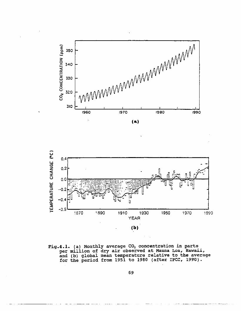
-.EQ, 350Q,
zo 340I-<[a:::;-
~ 330uzo~. 320ou
1990198019701960
310 "---I.__---1__......Jl..-__"--__J.-__~__.LJ
(a)
i99Q
.. -
197019501910 1930YEAR
~890
O,4r------------------------,wC)
Z<tJ:U
wa::=:l
~a::wa.:E~ -0.5'-------'-----------------------J
uo-
(b)
Fig.4.1. (a) Monthly average CO2 concentration in partsper million of dry air observed at Mauna Loa, Hawaii,and (b) global mean temperature relative to the averagefor the period from 1951 to 1980 (after IPCC, 1990).
69

longshore and cross-shore directions by nearshore currents
and waves. At most Hawaiian beaches surrounded by wide
fringing reefs, longshore sediment transports, in general,
are not so significant since waves usually break over the
wide and shallow nearshore reefs before they approach the
beaches. At beaches between headlands, such as Waimea
Beach, the longshore transport causes a reorientation of the
beach with changing wave conditions (Gerritsen, 1978).
A simplified two-dimensional 'relationship between sea
level rise and cross-shore sediment transport' was first
suggested by Bruun (1954) (the Bruun Rule), and widely
tested and modified by other authors and by himself
(Schwartz, 1965, 1967; Dubois, 1975; Dean and Maurmeyer,
1983; Bruun, 1988). For long-term change of sea level and
coastal erosicn due to cross-shore sediment transport, the
Bruun Rule is a widely accepted concept despite its
limitations in three-dimensional situations (Bruun, 1988).
Bruun (1962) proposed a simple two-dimensional
relationship between shoreline retreat and an increase in
local sea level along the cross-shore direction (Fig.4.2).
It is assumed that
1) the upp~r beach is eroded due to the landward translation
of the profile,
2) the material eroded from the upper beach is transported
and deposited offshore,
70
--------_._--- - -- -_._-----
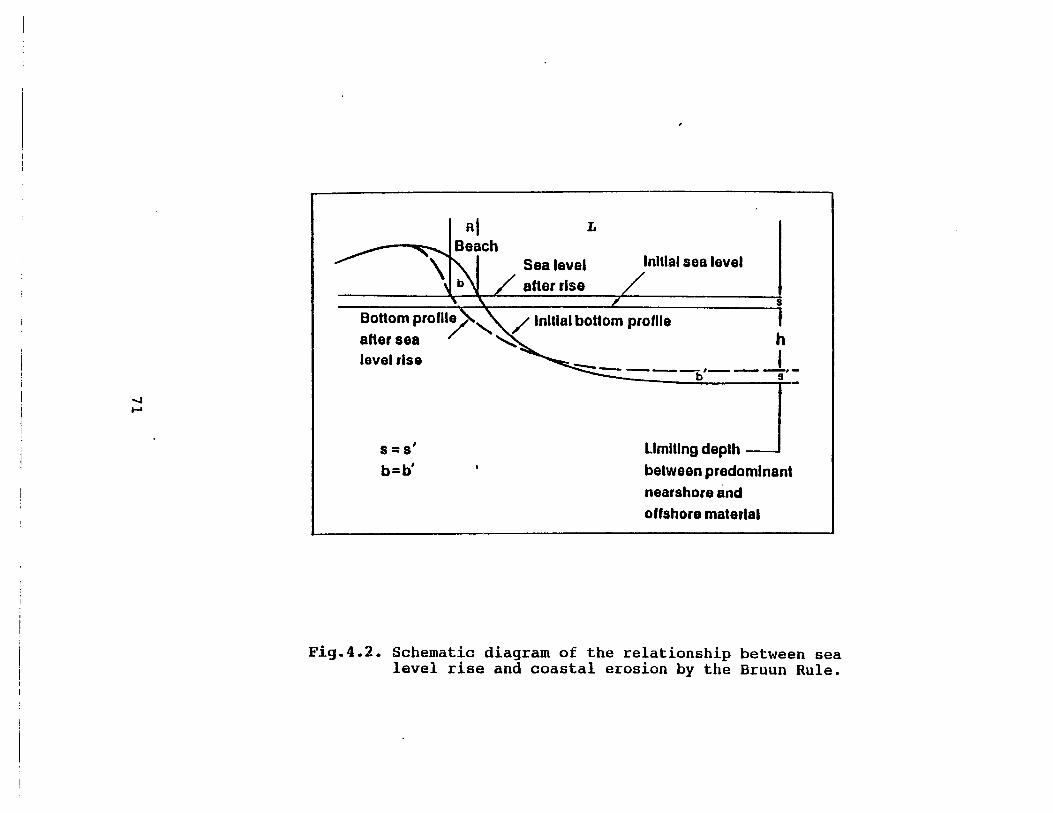
I~------,----,-b s
s
h
Initial sea level
L
Sea levelatter rise
Bottom profll/,," / Initial bottom profileahersea .~
level rise
......t-'
S=8'
b=b'Limiting depth
between predominantnearshore andoffshore material
Fig.4.2. Schematic diagram of the relationship between sealevel rise and coastal erosion by the Bruun Rule.

3) the rise in the nearshore bottom as a result of this
deposition is equal to the rise in sealevel, thus
maintaining a constant water depth.
When the gradient of longshore sediment transport is
negligible, the eroded volume of sediments must be balanced
by the volume to elevate the active width of the profile L,
and a vertical distance (i.e., sea-level rise) S such that
R = L * S ::B+h
stancl>
(4.1)
where R = the shoreline retreat rate,
S = an increase of sealevel,
L = the cross-shore distance to the water depth (h)
of effective motion,
B = berm height,
tan cI> = (B + h)/L ; the average slope of the nearshore
along the cross-shore width L.
Meanwhile, Dubois (1975) defines tan cI> as the nearshore
slope seaward from breaking waves, instead of the slope from
the shore to the 'depth of effective motion'. In general,
the bottom profile is not smooth and the 'depth of effective
motion' may be variable, especially depending on the time
scale of interest. But Dubois' definition does not seem to
be a reasonable alternative, although it is validated by his
72

quantitative analysis, because a great portion of sediment
transport occurs within the surf zone and hence the bottom
profile in the surf zone may be more important than the
slope seaward from the breaker line. Definitely, it must be
the average slope, that is, 'effective vertical dimension
over effective horizontal dimension of active profile'.
Dean and Maurmeyer (1983) suggested the modified Bruun
Rule by considering the third dimension in the longshore
direction:
(4.2)
where P = decimal fraction of eroded material that is
compatible with the surfzone sediment, and
GB = sediment-budget terms including contributions
from rivers or offshore, losses due to
sediment being blown inland or transported
offshore, and the longshore gradient of the
littoral drift.
That is, the amount of littoral sediment drived from
shoreline recession is balanced by the sum of the quantity
required to maintain the equilibrium profile relative to a
sealevel rise (L*S) and the sediment-budget terms (Ga ) .
73

A basic assumption of the Bruun model is the existence
of an 'equilibrium beach profile', and that this profile is
maintained or eventually achieved following a change in
water level. The concept of 'equilibrium beach profile'
(Bruun, 1954~ Dean, 1977~ Bodge, 1992~ Pruszak, 1993) may be
defined as an idealization of conditions which occur in
nature for particular sediment characteristics and steady
wave conditions (Dean and Maurmeyei, 1983). If a beach has
a specific grain size and is exposed to constant forcing
conditions, the beach may develop a profile shape that
displays no net change in time (Larson, 1991). But 'the
profile shape with no net change in time' may be different
from beach to beach even for the same grain size and for the
same wave conditions if the underlying geology, i.e., the
bottom resistence against the forcing, as described by
Pilkey et ale (1993), is different or if the component of
the beach sediments is carbonate rather than silicate. In
order to reach the same equilibrium state in beach profile,
whether kinetic or dynamic, not only the forcing (in waves
and sea level fluctuations) but also the response (in grain
size, origin of sediments, and underlying geology etc.)
should be the same.In reality, the equilibrium profile is
dependent on wave contions, and the evolution of a beach
profile from one state to another does not occur with a
constant profile form because the changes of profile are
initiated where the profile is the most out of equilibrium.
74

Bruun (1954) and Dean (1977) propose an equilibrium
beach profile given by
hex) = A x m
where h(x) = water depth
x = horizontal distance from shoreline
A = dimensional shape parameter
(4.3)
Dean (1977) shows that eq.(4.4), with m = 2/3, is consistent
with uniform energy dissipation per unit volume across the
surf zone, applied to the u.s. east coast and the Gulf of
Mexico.
Bodge (1992) suggests an alternative expression for the
equilibrium beach profile given by
hex) = B (1 - e-bx) (4.4)
where 'two parameters Band b have dimensions of depth and
distance-1, respectively. He compared eq.(4.3) and eq.(4.4)
for various profile data and for hypothetical profiles, and
concluded that the exponential expression eq.(4.3) is a
better approximation to fit the data, especially for beaches
with decreasing grain size in the offshore direction.
75

Bruun's (1954) empirical relationship (eq.(4.3)) from
the beach profiles at Mission Bay, California and on the
Danish North Sea coast was the first formulation for the
equilibrium beach profile. By applying a least squares
procedure, Dean (1977) proved that eq.(4.3), with m = 2/3,
statistically well represented about 500 beach profiles
(Hayden et al., 1975) along the u.S. east coast and the Gulf
of Mexico. This empirical relationship for equilibrium
beach profile has been used as the basis for the design of
most coastal engineering projects on the continental
beaches. In fact, the Bruun Rule (Bruun, 1962) is basically
a simple equilibrium profile model that assumes the constant
profile bounded by a 'closure depth'. The concept of a
'closure depth' (or a depth of effective sediment motion) is
a critical assumption such that there is no net transport of
sediment beyond the depth. The offshore current activity
capable of transporting sediment beyond the closure depth
was recognized as an insignificant and probably slow process
(Bruun, 1962). But Pilkey et al. (1993) claimed that the
concept of a closure depth is not valid since the offshore
transport of sands beyond the closure depth is not
insignificant during the last 20 year history of sand
replenishment from Wrightsville Beach, North Carolina.
Instead, they suggest the 'regime profile' concept to fit
reality for certain beaches.
76
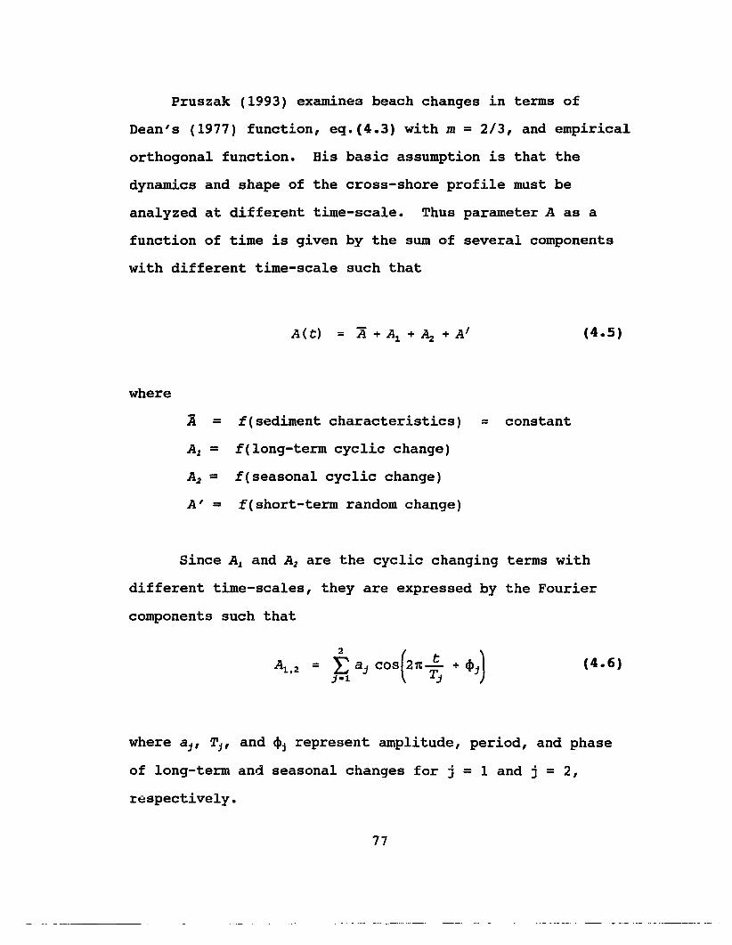
Pruszak (1993) examines beach changes in terms of
Dean's (1977) function, eq.(4.3) with m = 2/3, and empirical
orthogonal function. His basic assumption is that the
dynamics and shape of the cross-shore profile must be
analyzed at different time-scale. Thus parameter A as a
function of time is given by the sum of several components
with different time-scale such that
(4.5)
where
A =
Al =A2 =A' =
f(sediment characteristics) ~ constant
f(long-term cyclic change)
f(seasonal cyclic change)
f(short-term random change)
Since Al and A2 are the cyclic changing terms with
different time-scales, they are expressed by the Fourier
components such that
(4.6)
where aj' Tj , and ~j represent amplitude, period, and phase
of long-term and seasonal changes for j = 1 and j = 2,
I:'espectively.
77

A wave-based profile zonation comes from the
exponential distribution form of wave statistics. And the
peak near-bottom velocity that is exceeded 12 hours per year
(~ 0.14%) is given by
(4.7)
where de = closure depth with a seaward limit to extreme
surf-related effects throughout a typical year
P. = density of sands
P = density of seawater
The closure depth (de) for quartz sand in sea water with
small-amplitude wave theory is approximated by
(4.8)
In any case, a closure depth must be the key concept in
equilibrium profile models, which were developed for
siliceous continental beaches. However, calculating a
closure depth for calcarious Hawaiian beaches with the
equilibrium profile model is still useful.
78
The maximum and minimum values of significant wave
heights throughout a typical year at the NOAA buoy location
are 6.9 m and 1.1 m, respectively, and the median and
standard deviation are as follows:
Hs50 ==
4.0 m
±0.95 m
Then, the closure depth by eq.(4.8) is obtained as
= 2 Hs50 + 12 as.
20 meters
This value is larger than the annual depth of effective
motion which was estimated roughly twice the extreme
nearshore wave height exceeded 12 hours per year
(Hallermeier, 1981a). At Waimea Bay Beach, Oahu and at
Hapuna Beach, Hawaii, the approximate depth of seaward limit
to intense cross-shore sand transport was about 15 meters
for model-storm waves in this study. This value of the
closure depth is about 25% smaller than that calculated by
eq.(4.8). The descrepancy may come from either
underestimate by the Bailard's model or overestimate by
eq.(4.8) because nearshore wave height is usually higher
than deep-water wave height due to shoaling.
79

In reality, the depth of effective motion may depend on
the time scale of interest. For example, at some locations
on the east coast of the u.s. the effective depth associated
with periods of interest of 1 year, 5 years, and 20 years
may be about 4.5 m, 6 m, and 7.5 m, respectively (Dean and
Maurmeyer, 1983). For longer time-scale of interest, not
only waves but also sea-level fluctuations should be
considered as forcing functions to the beach erosion.
Moreover, the longer the period of sea-level fluctuations
the more effective it may be on beach erosion if longshore
sediment transport and all the other factors are negligible
(that is, if cross-shore transport is the only significant
erosion/acretion process).
Komar et al. (1991) argue that, if water-level is
rapidly changed such as an abnormal sea level rise during an
EI Nino, the response of the beach may be too slow to
maintain the equilibrium profile. Some other authors
(Edelman, 1968; Dean, 1977; Kriebel and Dean, 1992) applied
the Bruun Rule for shorter time-scale change of beach
profiles. Therefore, it is controversial whether the Bruun
Rule may be justified for investigating short-term
variations.
Sea-level rise never occurs in a steady manner but in
fluctuations with different time-scales. In fact,
80

interannual sea-level fluctuations seem to be very important
to coastal processes and shoreline retreats since the RSL
fall after the rise in this time-scale cannot usually
restore the lost amount of the sediments as is the case of
the mean annual oscillation of the cross-shore transports.
Hence the computation of only long-term shoreline recession
according to the Bruun Rule definitely underestimates the
real amount of coastal erosion. Moreover, longshore
sediment transport often plays a significant role in local
shoreline changes. Thus, the relationship between sea-level
rise and coastal erosion must be examined at least for an
isolated beach or a littoral cell where there is little net
longshore sediment transport to and from neighboring
beaches. Despite the controversy of the validity of a
closure depth in equilibrium profile models, a seaward limit
to the effective sand motion by waves has been applied to
many engineering problems.
81

CBAP~ER 5
~BE EFFEC~S OF S~ORMS ON BEACH EROSION
5.1. GENERAL REMARKS
The cross-shore sediment transport due to waves is
caused by
1) onshore transport by asymme~ry of wave for.m in shallow
water,
2) offshore transport by the return flow under the trough of
wave form due to continuity, and
3) offshore transport as a bedload due to gravity at the
bottom.
~~~ water level
..................
onshore transport.. . .. .. .. . ..
Fig.5.1. Schematic diagram of cross-shore sedimenttransport processes under waves. Arrows representaverage transports over a wave period.
82

Linear gravity wave theory gives the phase speed of a
small-amplitude deep-water wave as
.9k
(5.1)
The second order Stokes wave moves slightly faster than the
linear small-amplitude wave, which can be expressed in terms
of the wave steepness, i.e., the ratio of wave height to
wavelength (= B/l) (see Fig.5.2-1, Kinsman, 1984),
(5.2)
The real trajectory of a fluid particle is not a closed
circle such as described by pure linear wave theory but an
open circle resulting in a nonzero mean second-order drift
arising from the nonlinear solution (Stokes drift), which
represents the difference between Lagrangian and Eulerian
velocities.
Actual wave fields in shallow water show an extreme
aSYmmetry (or nonlinearity) of wave form. The consequence
of it is that the onshore fluid velocity under the crest of
the wave is greater than the offshore-directed velocity
83

underneath the wave trough, resulting in an onshore sediment
transport.
Return flow (or undertow) occurs between wave trough
and the bottom, forming a vertical circulation cell due to
the conservation of mass, while rip-currents form a part of
a horizontal circulation cell. Thieke and Sobey (1990)
considered the conservation of mass, momentum, and energy to
describe cross-shore mean flow circulation with the
horizontal flow velocity in terms of three components: a
time-averaged quantity, turbulence and waves. They show
that the return flow is rather less intense and directed
offshore while the wave-induced mass transport velocity
between trough and crest of the wave is relatively intense
and directed towards the beach.
Once the near-bottom flow velocity exceeds the sediment
threshold velocity, bottom sediments move as bedload by the
resultant forces of gravity and friction.
During high and steep wave conditions, sediments move
offshorewards due to the relatively stronger return flow
than the onshore transport by wave asymmetry (erosion). The
eroded sediments often form longshore bar(s) to the offshore
region. During low and mild wave conditions, sediments move
in the reverse direction (accrection) due to the wave
84
.. _.._-- -----

asymmetry and the relatively weaker return flow. The
longshore bar is basically unstable and often migrates with
the nodal point of infragravity waves (or surf beat), the
uncoupled low-frequency waves in the nearshore region
(Gerritsen and Jeon, 1991).
Waves around the Hawaiian Islands can be generated by
both local and remote wind fields in any part of the Pacific
Ocean. Trade winds (northeasterlies to southeasterlies) are
predominant over almost the whole year since the Hawaiian
Islands are located in the middle of the trade wind belt,
which generates trade-wind waves. Kona storms (southerly to
southwesterly) due to the passage of extratropical low
pressure systems associated with the westerlies during
winter (from October to April), although not frequent, cause
Kona-storm waves. Remote storms from the Aleutians or mid
latitudes in the North Pacific and from the Southern
Hemisphere generate North Pacific swell and Southern swell,
respectively. Each swell is usually frequent during the
winter time of each hemisphere (Inman et al., 1963; Moberly
and Chamberlain, 1964) (Fig.S.2).
The surf condition on the north shore, Oahu is
extremely variable, usually very low during summer and very
high during winter. The mean surf heights in summer (June,
July, and August) and in winter (December, January, and
February) on Sunset Beach were 0.11 + 0.11 m, and 2.35 ±
85

ISLANDS~
~~
349"·....-----
HAWAIIAN ~21
CN+
1sa-w
2S1·
frNo
? ~O 190 110
Kilometers
Fiq.5.2. The ranges and mean directions of the typicalwind waves approaching to the Hawaiian Islands(Inman et al., 1963). .
86

1.35 m, respectively, during 1988 to 1992. Maximum surf
height was reported over 7 m during the same period.On the
contrary, mean surf heights on the south shore, Oahu are
fairly low in both seasons but a little higher in summer (Hb
= 0.90 ± 0.33 m) than in winter (Hb = 0.63 ± 0.27 m).
Maximum wave height off Diamond Head, Oahu during this
period was reported about 2.1 m. Meanwhile, the condition
on the west shore, Oahu is in between north and south
shores. Mean surf height on Makaha Beach was 0.35 ± 0.35 m
in summer and 1.31 ± 0.90 m in winter, and maximum height
was 6.1 m during the same period (Fig.S.3). This is because
the surf condition is highly correlated with the winds
the North Pacific storms in winter and the trade winds
during the rest of the year -- in the Hawaiian Islands.
Wave-induced longshore currents due to breaking result
in longshore sediment transport, which will not be discussed
in this study since longshore transport is often not
significant at Hawaiian beaches. Shallow coral-reef
environments often play a role as offshore breakwaters and
wave energy is greatly reduced before it arrives at the
shore. This study is strictly limited to the shoreline
change due to cross-shore sediment transport. However, edge
waves and surf beats (or infragravity waves) are often
responsible for many coastal features such as beach cusps,
crescentic bars, caps, and bays.
87
-- .---- ----

400Diamond Head (winter)
150
,->.
300u=1.1 100:::2
2001-a-1.1
ol::I-
... 50100
00=
00 1 2 3 4 °0 1 2 3 4
surf height [m] surf height [m]
tDiamond Head
Sunset
8246surf height [m)
Sunset Beach (winter)
--i:--
h
200
150
100
50
00
31 2
surf height [m)
400>.ucu:::2a-u
ol::...00c
300
surf height
500 Sunset Beach (summer)
~
4OO,--=,=:;:;':;::":':;:==-~=:::.L---,
300
200
100
00 . 1
1 2
surf height [m]
3
Fig.5.3. Surf height distributions on Diamond Head,Makaha Beach, and Sunset Beach, Oahu in winter(December, January, February) and in summer (June,July, August). Data are from P. Caldwell, TOGA SeaLevel Center, Univ. of Hawaii.
88
Rip currents play an important role as a secondary
return flow in nearshore circulation. They carry water back
to the offshore region through the breaker zone in
horizontal circulation, often with an undulating shoreline.
They appear most noticeable when long and high waves produce
wave setup on the beach (U.S.Army Corps of Engineers, 1984).
Wave climate northwest of Kauai (see Fig.3.2. for the
location of the NOAA buoy) is shown as annual variations of
daily mean significant wave heights for 12 years in Fig.5.4
(~ach curve represents an annual time-series each year). The
average of significant wave height in winter (December,
January, and February) exceeds 3 m, while it is reduced to
less than 2 m during summer (June, July, and August). The
corresponding average wave period is about 2 seconds longer
in winter than in summer (Table 5.1). This is because
stronger North Pacific swells affect the wave climate during
winter and milder trade-wind waves prevail during the rest
of a year (Inman et al., 1963; Moberly and Chamberlain,
1964; Patzert, 1969). From the crude correlation analysis
between local wind directions and waves at the NOAA buoy
station, North Pacific swells occur only about 5% of the
annual time-series of waves while trade-wind waves occupy
about 80% of the year. Southern swells and Kona-storm waves
occur during the remaining 15% of the year.
89
----_.--- .. ----- ------ -----

10
- 9a~
8o6J..dtJ\ 7·rotQ).d
6Q)
~ 5:-o6J
4c::\0 cd0 0•rot
'H·ri~tJ\ 2·rotII)
1
00 50 100 150 200 250 300 350
(Julian days)
Fig.5.4. Wave climate as annual variations of daily meansignificant wave height for 12 years at the northwestof Kauai (23°24'N, 162°18'W), measured from the NOAAenvironmental buoy (no. 51001). Data are from NODC.

Table 5.1. Averaged significant wave height and wave periodby season and by wave type: winter (December, January,February) and summer (June, July, August) seasons dataare averaged from 1981 to 1992, and different wave typesare taken in 1985 and 1990, at the NOAA buoy (51001)location (23°24'N, 162°18'W).
============================================================season
or wave typeaveraged
sig. wave height (Ho )
averagedsig. wave period
winter 3.1 + 0.17 m 7.7 ± 0.5 secsummer 1.9 + 0.11 m 5.7 ± 0.4 sec
Trade-wind waves 2.4 m 6.5 secSouthern swells &
Kona-storm waves 2.8 m 7.7 secNorth Pacific swells 3.5 m 8.0 sec
Disastrous damages as well as erosion of low-lying
coastal areas may result from tropical cyclones and tsunamis
(or seismic sea waves).
The typical horizontal dimension of a hurricane is
about 200 km or less, and maximum wind speed near the center
is about 50 to 100 m S-l. The paths of hurricanes are
largely controlled by the subtropical high pressure areas
over the oceans. Initially they move westwards at low
91

latitudes in the prevailing easterlies, but then often curve
polewards around the high pressure center and finally travel
in an easterly direction under the influence of the westerly
winds of high latitudes (Harvey, 1976).
The frequency of tropical cyclones passing over a
specific area is relatively low. Gray (1979) reviews a
brief discussion of the character and the effect of the
tropical cyclones on the ocean. He found a world average of
80 events per year during a 20 year period (Fig.5.5). They
originate in latitudes between 5° to 25°, not at the equator
where the Coriolis effect vanishes, but only in longitudes
in which the sea is warm, thus allowing
the equivalent potential temperature at the surface to reach
values high enough for strong convection to be promoted
(Gill, 1982).
When tropical storms over very warm surface water
(> 26°C) are rapidly amplified into intense vortical storms
by a certain mechanism10 under favorable conditions of
moisture supply, they become tropical cyclones such as
hurricanes or typhoons (Holton, 1979). Thus hurricanes
occur more likely during summer season. In fact, more than
10 Conditional Instability of the second Kind (CISK) -- theprocess of the cooperative interaction between the cumulusconvection and a large-scale perturbation leading tounstable growth of the large-scale system.
92

70 % of the total tropical cyclones of the Northern
Hemisphere during 1958 to 1977 were reported between July
and October (Gray, 1979).
The oceanic response to the passage of a hurricane or
depression is basically dependent upon the hurricane speed
(U) relative to the long gravity-wave speed (c); for a slow
moving disturbance (U < c), the atmospheric pressure and the
water displacement are out of phase and the response of the
ocean is confined to the neighborhood of the hurricane. For
a fast-moving disturbance (U > c), which is the more usual
situation in nature, the pressure and displacement are in
phase and the amplified lee waves appear behind the
hurricane. When both speeds are the same (U = c), the
response has the same shape as that of the forcing (Gill,
1982) •
Hurricanes which directly hit the Hawaiian Islands
such as Nina in 1957, Iwa in 1982, and Iniki in 1992 during
a few recent decades (Fig.5.6) have caused great damage and
coastal erosion due to the direct storm effects and the
surges running up the coastal regions. Unfortunately, no
direct measurements of beach profile changes have been taken
before and after the hurricanes.
93

fir
V
.,
II>'
\0or:-
=r "" 81 ., ,,-r I.,
Fig.S.S. The location of the points of origin of tropicalcyclones during a 20-year period. (after Gray, 1979)

Run-up height is of particular interest to coastal
engineers because it gives the upper limits of inundation of
the coastal region and also affects the design and
construction of coastal structures.
Bunt (1959) proposes an empirical relationship of the
runup height (Ru ) to wave height (Hb ) , deep-water wavelength
(Ao ) , and beach slope (= tan p) such that
e ,
Ru = .[llb'A;, tanp (5.3)
The relative runup height (Ru/Hb ) may be expressed by
(5.4)
The right-hand side of eq.(S.4) is also called 'surf
similarity parameter'. Its value determines breaker
type11, wave runup, and stability of breakwater units. As
an engineering application for a coastal structure, run-up
height can be reduced by increasing the roughn~ss and
permeability, decreasing the slope, and changing the shape
of the structure into a 'berm structure'.
11 Four common classifications are spilling, plunging,collapsing, and surging breakers (after Galvin, 1968).
95

180"
:4 Fico:. Jul i9
•• •• I -,~
.'{'....
\I
PACIFIC OCeAN
Tropical disturbance .Tropical depression .
Tropical storm -----Hurricane -
-. HawaIian~:- Islanas
~
Fig.5.6. Hurricane tracks around the Hawaiian Islands
96

5.2. SHORT-TERM BEACH EROSION MODELS
Bailard (1984) generalized an energetics-based sediment
transport model which had been originally developed for
streams by Bagnold (1966). This model is useful for short
term changes of the beach profiles due to its simplicity.
The resulting equation for local longshore and cross
shore transport rates is expressed as functions of local
waves, currents, and sediment parameters such that
where = instantaneous sediment transport rate
(5.5)
Ut = instantaneous near-bottom fluid velocity
CL = drag coefficient of the bed
eb = bedload efficiency factor
es = suspended load efficiency factor
tan p = bed slope
~ = internal angle of friction for the sediment
Ws = fall speed of the sediment
p = density of the fluid
i = unit vector directed upslope
< > = time-averaged quantity
97

The above sediment transport rates imply the feature
that the bedload and suspended load transports consist of
primary components directed parallel to the instantaneous
fluid velocity vector, and secondary components directed
downslope.
Total '(near-bottom) velocity u, is split into an
oscillatory and a steady velocity components such that
Ue '" (acose + u) 1 + (a sine + v):J (5.6)
And the oscillatory velocity is expressed by the harmonic
components such that
a ::: U. cosat + u~ cos2at + ••• (5.7)
With the assumptions that
1) a steady velocity component is relatively small with
respect to the maximum amplitude of an oscillatory
component (u/ u,. « 1),
2) incident wave angle is nearly orthogonal to the shoreline
(cos a == 1),
98

both local and (spatially) averaged longshore and cross
shore transport rates are obtained.
The resulting cross-shore transport equation becomes
where
=
(5.8)
(5.8.1)
u; = <lu,J')u;
(5.8.2)
(5.8.3)
The relative mean velocity ~u and the wave velocity
moments '1' V2 can be estimated from the measured field
data and correlation with incident wave characterisitics.
But u/ and u/ are assumed to be constants following
previous results (Guza and Thornton, 1981; Bailard, 1984).
99

The oscillatory component of the fluid velocity
includes both short-period (incoming) waves and longer
period (reflecting) infragravity waves, and hence simple
Fourier decomposition may not be sufficient to express the
oscillatory component.
It seems worthwhile to review Roelvink and Stive (1989)
although their idea is not applied in this study. The
oscillatory component of the total wave velocity may be
decomposed into short and longer waves, that is,
a (5.9)
They discuss the wave velocity moments in terms of
these two components. Assuming that 1) the individual
waves, u, are not correlated to 1UL 12 and IUL 1J, and that
2) uL« U." they obtain the odd central flow moments
such that
(5.10)
(5.11)
100

The first terms on the right-hand side are nonzero when
there exists an asymmetry about the horizontal plane caused
by nonlinearity of the waves. The last terms are nonzero if
there exists a correlation between the slowly varying
velocity uL and the short-wave velocity variance u,/. They
use separate models for the first and last terms according
to a nonlinear, monochromatic theory and a wave envelop
interaction for a bichromatic wave train with accompanying
bound long wave, respectively.
Despite the simplicity, Bailard's model for cross-shore
sediment transport shows some realistic features such that
1) gradual onshore sand movement occurs when waves are
small, while rapid offshore movement occurs with larger
waves.
2) the equilibrium wave height is small with steep beaches,
while it is larger with flat beaches.
3) a beach adjusts to an equilibrium beach slope with the
incident wave height over sufficient time.
The limitations of the energetics-based model are that
it does not include sediment threshold of motion effects, a
variable drag-coefficient, and a different formulation for
the rate of energy dissipation in the surf zone.
101
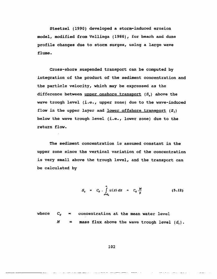
Steetzel (1990) developed a storm-induced erosion
model, modified from Vellinga (1986), for beach and dune
profile changes due to storm surges, using a large wave
flume.
Cross-shore suspended transport can be computed by
integration of the product of the sediment concentration and
the particle velocity, which may be expressed as the
difference between upper onshore transport (5u ) above the
wave trough level (i.e., upper zone) due to the wave-induced
flow in the upper layer and lower offshore transport (51)
below the wave trough level (i.e., lower zone) due to the
return flow.
The sediment concentration is assumed constant in the
upper zone since the vertical variation of the concentration
is very small above the trough level, and the transport can
be calculated by
where =
Cd • J u(z) dz :::z.de
concentration at the mean water level
(5.12)
M = mass flux above the wave trough level (dt ) .
102
.- .._.- -_.----_.-. ---_ ..__._.--...._ ..
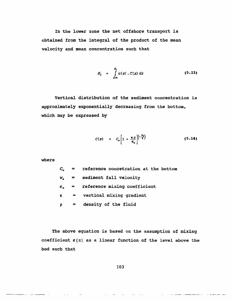
In the lower zone the net offshore transport is
obtained from the integral of the product of the mean
velocity and mean concentration such that
dt
81 '" JU(Z) • C(Z) dz:r-O
(5.13)
vertical distribution of the sediment concentration is
approximately exponentially decreasing from the bottom,
which may be expressed by
where
C(z) '" Co [J. + ~:t :-)
Co = reference concetration at the bottom
w'" = sediment fall velocity
eo = reference mixing coefficient
K = vertical mixing gradient
p = density of the fluid
(5.14)
The above equation is based on the assumption of mixing
coefficient e(z) as a linear function of the level above the
bed such that
103
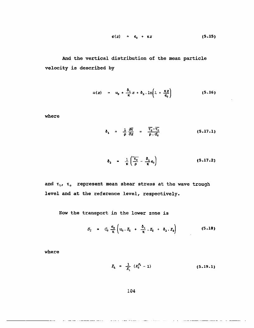
e(z) (5.15)
And the vertical distribution of the mean particle
velocity is described by
where
u(z) ~l (lCZ).. Uo + - Z + ~Z • In J. + -lC eo (5.16)
= (5.17.1)
..!. ('to _~eo)lC P lC
(5.17.2)
and ~t, ~o represent mean shear stress at the wave trough
level and at the reference level, respectively.
Now the transport in the lower zone is
(5.18)
where
(5.19.1)
104

(5.19.2)
(5.19.3)
and
(5.19.4)
As an application of the Bruun Rule to a short-term
scale, Edelman (1968) proposed a beach-response model before
and after a storm with a constant equilibrium profile
relative to the instantaneous sea level and a uniform slope
depending on sediment characteristics. He assumed the wave-
breaking depth as the depth of effective motion. He
attempted to generalize the dune erosion as a function of
storm surge level and dune height (Fig.5.7).
105

R
F•• 0"0 •
O.oo.iliOnEquilibrium S'orm Profil.
; ..
Slorm Tid. l..v.1 e:roSlon ::: .--------------- -=~~~: DMlan Sea ~.v.1 _.......-----:- .~.".':'"
(0) Ed.lman's M.'had I Appli.d '0 Id.alized B.och Profile.
10 r--..,..----r--r--~--r__-..,
_ a---en
iii 69I-
2 4II:oI-en Z
...-D I 20 f' ~.,..,.,.. D 110 ft
-z~
//Ii
300100 200DUNE RECESSION. R ( ft )
O'---"'--'""'-_-I-_......._--I._~o
(b) Dune Erosion Versus Storm Tide forIdealized Profile. FlO. Hb "tS S.
Fig.5.7. (a) Schematic diagram of the Edelman's (1968)model for an idealized beach profile, and (b) therelationship between dune erosion and stor.m-surgeheight.
106

5.3. SHORT-TERM FLUCTUATION
Short-term events in the order of a few hours to days
by tropical storms, hurricanes and tsunamis may worsen the
erosion problem since the frequency and severity of the
storm surges and the seismic sea waves with rising sea level
may be higher and stronger than those at present (IPCC,
1990), and the coastal inundation limit may be further
inland. The major damage and loss of life from most
hurricanes occur within 100 to 150 km of the landfall
position, the point where the low-pressure center crosses
the coastline (Fig.5.8). vertical rise of sea level by
hurricanes commonly reaches more than 4 m above the MSL,
especially on the continental coasts. The tide-gauge
record by hurricane Camille in 1969 rose up to a peak-height
of 7.5 m around the Gulf of Mexico (Simpson and Riehl,
1981). Although the peak height of sea level on the
Hawaiian coasts is not so high as on the continental coasts,
tropical storms and hurricanes, may still cause great
erosion on the Hawaiian beaches. The effect of the
extremely raised sea level due to a big storm usually
continues a few days even after the storm passes through.
The frequency of tsunamis (or seismic sea waves) in
Hawaii is higher than that of hurricanes; the wave period is
less than an hour. Thus their direct effect on beach
erosion mayor may not be significant. But tsunamis are
also accompanied by an oscillatory wave train.
107
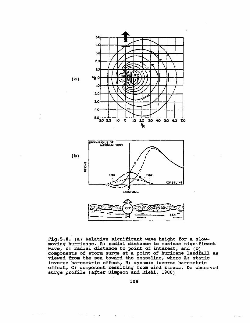
~.Or--,..-.,-...t-.,.--.,r--..,..-r--....,..-.,-.....
4.0t--+--~=2~+-~f--+-~~-l--4-~
1.0
( a)
2.0t-~~r:looci"~""'''''9-~o:.1--I-~+-++---i
3.01--+~d-~~+-'-"-~~-~'-"~
4.0t--+--+--=f~-+--1--+-~f'--+--+--i
~'°3.0 2.0 1.0 0 1.0 2.0 3.0 4.0 0.0 6.0 7.0
~R
RMW-RAOIUS OFMAXIMUM WIND
(b)
o
COASTLINE
---'----- st.. -
Fig.S.8. (a) Relative significant wave height for a slowmoving hurricane. R: radial distance to maximum significantwave, r: radial distance to point of interest, and (b)components of storm surge at a point of huricane landfall asviewed from the sea toward the coastline, where A: staticinverse barometric effect, B: dynamic inverse barometriceffect, C: component resulting from wind stress, D: observedsurge profile (a~ter Simpson and Riehl, 1980)
108
The convolution method (Kriebel and Dean, 1993) gives a
simple qualitative result for short-term beach erosion,
which is based on the ratio of the erosion time scale to the
storm duration. That is, storm duration plays a part in
determining the maximum erosion response since the
characteristic·time-scale of beach erosion (T.) does not
change much, which is a function of beach-face slope,
breaking wave height (Hb ) , and sediment fall speed (w.) (see
eq.(S.20»). Dean (1987) shows that the parameter A in an
equilibrium profile with 2/3 power law is a function of
sediment fall speed or grain size (A ::: (w//g) 1/3) •
The erosion time scale (T.) from the numerical model is
given in the form:
where
(5.20)
C·
=
=
wave height at breaking-point,
empirical coefficient fitted from numerical
tests.
They assume that the beach response to steady-state forcing
conditions is approximately exponential in time such that
109

(5.21)
where
T. = characteristic time scale of the exponential response,
R. = maximum response of the contour (advance or retreat)
that occurs after the system reaches equilibrium.
For a linear beach slope joining the power-law curve as
h = A x2/3 (Dean, 1977), Kriebel and Dean (1993) propose the
maximum erosion potential from the conservation of eroded
and deposited sand volumes (see Fig.5.9) such that
R.. ::: (5.22)
where S = sea level rise
B = berm height
m = linear beach-face slope
h b = water depth at wave-breaking point
X b = surf-zone width
110
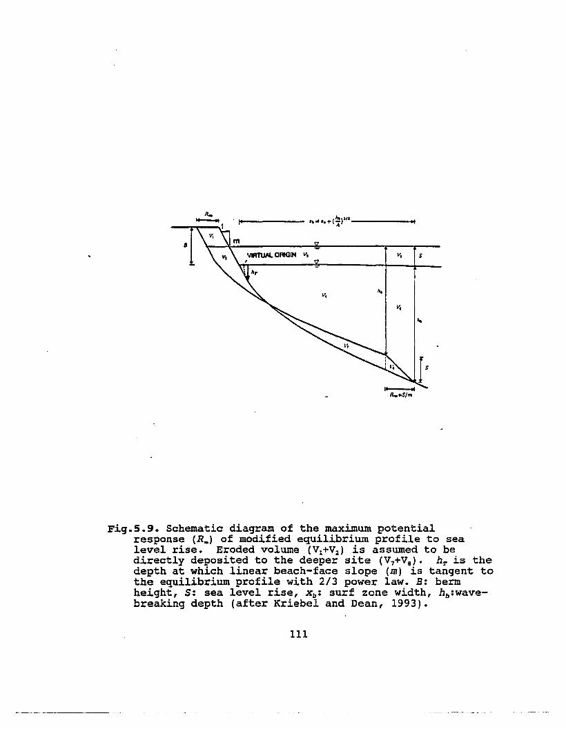
R..__ .1..------ '" (h,)J11 --I--r"'f'-'~1 ..... %. %. + A
B
Fig.5.9. Schematic diagram of the maximum potentialresponse (R.) of modified equilibrium profile to sealevel rise. Eroded volume (V1+V2 ) is assumed to bedirectly deposited to the deeper site (V,+Va) . h T is thedepth at which linear beach-face slope (m) is tangent tothe equilibrium profile with 2/3 power law. B: bermheight, S: sea level rise, x b : surf zone width, hb:wavebreaking depth (after Kriebel and Dean, 1993).
III
The time-dependent recession of each contour can be
approximated by the convolution method such as
tJ
R1(t
j> '" ~ R
1_ f f(1:) e-·(tr~l ch
o
where
(5.23)
index i is denoted for each sea-level elevation contour,
= characteristic rate parameter (= liT.), and
= measured storm-surge hydrograph at time t j •
For a characteristic erosion time-scale (T. = 18.5
hours) and an idealized storm by the sine-squared function
such that
(5.24)
maximum erosion occurs by about 10% of the erosion potential
for a typical hurricane (TD = 6 hours) near the end of the
storm, 40 to 75% of that for a typical storm wave (TD = 1
to 3 days), and about 100% for persistent northeasterlies
(TD = 1 month) with almost no phase lag, i.e., very close to
the time of the peak water level (Fig.5.10).
112
They have shown that this simple analytic model is in
good agreement with the numerical results for the
equilibrium response (Kriebel and Dean, 1985).
113

, , , ,
2.5
, , , , , , , , , , , , , , , , ,
-~---",?"O = 3 days
TO = 6 hrs
2
To = I day
1.5
.....
1
equilibrium
,,,,,,,,,,,,,,.,,,,,.',.-,,.,,
.',,,,,,,,,,
, '_:::_::_--------_:_------------------------------------------. 0.5
1
0.9
0.8
0.7
0.6
9
~ 0.5,-..-'-'~ 0.4
........ 0.3~
0.2
0.1
00
[radians)
Fig.5.10. Example of amplitude and phase lag of themaximum erosion (a) for a typical hurricane (TD = 6hrs), (b) for typical st~rm·waves (TD = 1 to 3 days),and (c) for persistent northeasterlies (TD = 1 month)with the erosion time scale of Ts ; 18.5 hra, in theHawaiian Islanda.

CBAPTBP. 6
SHORELINE CHANGES AND BEACH RECOVERY
6.1. SHORELINE CHANGES IN THE HAWAIIAN ISLANDS
Average yearly trends of accretion or erosion of some
beaches on the Islands of Kauai, Oahu, Maui, and Hawaii are
re-analyzed by taking into account the variation in
shoreline position due to the annual cycle in the mean sea
level (see Table 3.2 and Table A.2). Then, possible
reasons of shoreline dynamics on some selected littoral
cells as well as potential errors in calculating shorelines
from the previous papers are discussed (Hwang, 1981; Makai
Ocean Eng. and Sea Eng., 1991).
Accretion and erosion of beaches are significantly
related to the rising and falling trends of MSL. The
average linear trends of MSL will be compared with the
shoreline changes between two photographs at the same
location (time interval is from 5 to 20 years). For a few
selected beaches, shoreline changes are corrected with the
mean annual cycle of sea level and beach slope; the mean
annual cycle obtained from the 80 year time-series of
monthly sea levels at Honolulu Barbor can be applied to
correct the shoreline change at Waimea Bay, Oahu. In the
115

same way, the mean annual cycle from about a 40 year time
series of monthly sea levels at Hilo, Hawaii is applied to
correct the shoreline change at Hapuna Beach, Hawaii. This
assumes that the mean annual cycle of sea level of an island
is the same at any place on the island. The calibration of
the shoreline changes by interannual fluctuation of sea
level is not carried out in this study because it is
presently not known at what time of year the highest levels
occur in this cycle. Previous analyses of the coastal
erosion/accretion in the major Hawaiian Islands show average
annual changes based on aerial photographs within a few
decades of time (Fig.6.1).
The most serious erosion problems were reported on the
Island of Maui, especially on the north shore. More than 70
percent of the total number of transects were eroding. On
the Island of Oahu, Waimea Bay Beach (- 0.95 m/yr) had the
highest erosion rate. Meanwhile, maximum accretion was
reported on Kahuku Golf Course Beach (+ 1.14 m/yr), as the
result of sand dumping. On the Island of Kauai, erosion was
reported at about half of the transects. On the west to
northwest coast beaches of the island of Hawaii,
approximately 60 percent were reported as "eroding".
But there exists a large uncertainty both in
photographic measurements by an aircraft and in conversion
116

of the aerial photographs into base maps. The uncertainty
may reverse the mean annual trend of erosion/accretion if
the rate of shoreline change is not large. Moreover, when
two air photos were not taken in the same month the
positions of high water level (HWL), which is usually taken
as a shoreline in aerial photography, should be converted
into those of the same month to minimize error. Thus the
information of the beach slope should be incorporated for an
estimate of the shoreline position for the same month of the
year. An aerial photograph is an instantaneous snap-shot
and therefore cannot be representative for the shoreline in
that year.
Consequently, calibration of shoreline position should
be carried out, at least based on the mean annual cycle of
sea level and beach slope, by converting vertical sea level
change into horizontal shoreline change. But the
interannual shoreline changes cannot be accurately
calibrated up to now, due to the limited knowledge about the
prediction of occurrence of the interannual fluctuation of
sea level which seems to be largely associated with ENSO
events.
One of the most obvious and consistent features of the
sea level change in the world oceans is an annual
oscillation, which is primarily related to expansion by
117
-----------

2(a) Oahu Shoreline Changes
1 x
0 x:g x x w X X X _0 o ft 0 - 0 -
~0 x • x x ",-Q 000 x
-1 0
north windward south leeward-20 5 10 15 20 25 30 35 40 45 50
no. of sites
2( b) Hawaii Shoreline Chances
:g o ft 0 0 ft W X • v
~0 00 x .
x x " x.
xx
-1BA HB
-20 5 10 15 20 25 30 35 40 45 50
2(c) Maui Shoreline Changes
1 x x x
:g 00ft. ftO
X
0 0 . . 0 . x Xlr
~-00 " O""V 0oooQO - X xx.x x x•• x ° 00 00 0 ° 0 00
x' x0 X 000 0 0 0 0 x x
x 0 00 x
-1 x
MA MB Me x ,.x " MD
-2 .0 10 20 30 40 50 60 70 80 90
2(d) Kauai Shoreline CbanllCs
1 x00 0 x:g 0000
o 0 0 agO I .x- " "v 0 -0 0x!o...JI lI4.-v- 0
0 o x
8 0 " ...." .. Xll 0G 00°00 ogOOogaoa 00
0 "'J( 00 .. 'lCx- 00 00 0 0
0
-1KA KB KC KD KE KF
-210 20 30 500 40 60 70 80 90
Fig.6.1. Mean annual trend of shoreline changes (in m/yr)on (a) Oahu, (b) Hawaii, (c) Maui, and (d) Kauai.Data are selected from Hwang (1981) for (a), and MakaiOcean Eng. and Sea Eng.(1991) for (b), (c), (d)_
118

heating and contraction by cooling due to the annual
variation of solar radiation. Another predomimant cause of
an annual mean sea level oscillation in synoptic scale is
monsoons. For instance, Southeast Asian Monsoons over the
coastal regions of the western Pacific, which are primarily
northeasterly winds during the winter monsoon (from October
to April) and southwesterly winds during the summer monsoon
(from May to September), significantly magnify the amplitude
of the annual variation of the monthly mean sea level height
at the coastal stations (Jeon, 1990).
But the sea-level signals ~t the island stations away
from the coastal regions in the western Pacific are more·
complex than those at coastal stations. This is because
they may include several causes, as well as the steric
effect, such as the annual variations of the monsoon and
trade wind systems, and the intensity or spatial variation
of the equatorial current system, especially of the North
Equatorial Current (REC; between 10~ and 20~) and the
North Equatorial Counter Current (NECC; between 4~ and
10~) from the western to central Pacific Ocean.
Mean monthly sea levels in the .annual cycle at four
major Hawaiian Islands are shown in Fig.6.2. (also see Table
2.4). The annual cycle of sea levels implies that the rate
of shoreline change based on aerial photographs may result
119
_._-_._----

Nawiliwili Honolulu20 20
15 15
10
5
e '8 0~::~
~ ~ I !...-5 -5 I
-10 -10
-15 -15
-20 -205 10 5 10
( a) (b)
Kahului Hilo20 20
15 15
10
5 I -5
e 0 8"u u- "-
-5 -5II I
-10 I- - ~.- :-10f
-15 -15
·20 -205 10 5 10
( c) (d)
Fiq.6.2. Mean annual cycle of monthly sea levels atNawiliwili, Kauai, (b) Honolulu, Oahu, (c) Kahului,and (d) Bilo, Hawaii. Data are from PSMSL.
( a)Maui,
120

in a larger error range or even a reverse trend of
regression and/or transgression unless two air photos used
for calculating the shoreline change are taken at least in
the same month.
Suppose that one aerial photograph is taken in
September (maximum level) some year and the other in April
(minimum level) ten years later, and that the shoreline
between the two air photos is interpreted as "unchanged".
If we further assume that the beach slope is 1/20 and that
the long-term trend of sea level is +2 em/decade with an
annual MSL difference of 10 em at this coast, then the
shoreline may be interpreted as "retreated" by 1.6 m
(corresponding horizontal distance for the vertical rise of
8 em). Consequently, interpreting shoreline changes from
aerial photography without considering annual sea-level
oscillation may cause significantly erratic results.
Moreover, interannual sea-level fluctuation could certainly
cause the error to be even larger. It makes the prediction
of shoreline change difficult that the time span (as well as
the sea-level difference) of the interannual fluctuation is
somewhat variable, i.e., quasi-periodic.
If the vegetation line in aerial photography, which has
been usually represented for the shoreline in Hawaii, is
replaced by the mean HWL as used in the u.s. mainland, the
influence of season is as clear as in the above reasoning.
121

6.2 CASE STUDIES
6.2.1. Waimea Bay Beach, Oahu
Waimea Bay is located on the north side of the Island
of Oahu, and the beach is often subject to high surf
conditions from North Pacific swell (Fig.5.3). The Waimea
River, which is usually ponded behind a barrier of sand,
drains into the northeastern end of the bay in times of
flood (Parker, 1987). There is a sand channel extending
steeply into deep water opposite the river mouth, where the
offshore sand transport occurs by rip currents. Thus this
sand channel fed by rip currents may be an indicative of the
mechanism whereby sand moves permanently into deep water.
The bay is blocked on both sides by rocky cliffs, which
makes it a littoral cell where there is no net longshore
sediment transport to and from the area (Chamberlain, 1968).
Waimea Bay is chronically eroding with little sand
supply to balance the losses from sand mining (from 1949 or
possibly earlier to 1967) and offshore transport due to
winter storms (Hwang, 1981). But the long-term, annual or
interannual trends of sea-level rise may also be important
to beach erosion in this area.
122

N
I.....ii
i
",./
il
/i,
ri
2
,.-" ./",' ..-" /'. I
I •. I
" l/ /'
6 ./i .'
./ .'/' /
".' ,;" .,4_.....;. ".'"';"
/" :,,,
boulders
'"...... (.~ "
",.,/ '). ~._._.._._._.J (
......\\'. reels
\.'.'.
'..... .... ....
~/,/ .....; ...,......
i,.....10
/.
/;'
",;/ sandy bottom
",;'/...,.. . ,.........
o 100 200M
Fig.6.3. Waimea Bay Beach: geography and bottom topographyin the nearshore region (transects 2 and 3 arefor Table 6.3; transect 1 was not shown in Hwang,1981).
123

In previous analyses of the shoreline change from aerial
photos (Hwang, 1981), the rates of waterline recession may
not have been accurately estimated because of neglecting the
effect of the annual oscillation of mean sea level when the
photos have been taken in different months of the year.
The average values of the sediment sizes measured
along the beach profiles at (a) Waimea Bay, Oahu and (b)
Hapuna Beach, Hawai.i from previous reports (Moberly and
Chamberlain, 1964; Gerritsen, 1978; Parker, 1987) are as
follows:
Table 6.1. Average sediment diameter characteristics at theMLW line on (a) Waimea Bay, Oahu, and at (b) HapunaBeach, Hawaii. units are in mm and ~ (= - log2[mm])in parentheses.
(a) Waimea Bay, Oahu============================================================date 3/62
0.48(1.05 )
7/62
0.48(1.07)
10/62
0.74(0.43)
2/63
0.44(1.20)
5/63
0.57(0.80)
8/63·
0.61(0.72)
============================================================date
mm~
1/74
0.62(0.69)
2/74·*
0.61(0.72)
9/85
0.68(0.57)
1/86***
0.70(0.52)
(b) Hapuna Beach, Hawaii============================================================date 4/62 6/62 9/62 1/63 4/63 7/63* 12/73**
mm~
0.17(2.58)
0.17(2.56)
0.20 0.26(2.33) (1.94)
0.19 0.24(2.43) (2.04 )
0.26(1.94)
Data Sourcee;* 3/62 - 9/63 ; Moberly and Chamberlain (1964),
(Data were averaqed from three sitee; backehore, MLLW line, offshors.)** 12/73, 1174, 2/74; Gerritsen (1979) (data at the MLW line)*** 9/85, 1/86 ; Perker (1997) (data averaqed from &W, MW, LW)
124

More than 95% of beach sands on Waimea Bay, Oahu are
calcarious sand (CaC03 ) (Moberly and Chamberlain, 1964).
This implies that the terrigenous sediment supply from
occasional flooding of Waimea River is minor compared to the
biogenic component, and that much of the sand found in the
bay must be relict sands produced during a lower stand of
sea level (Campbell and Hwang, 1982). In general, the
primary source of sands of the Hawaiian Beaches is from reef
communities. After some Hawaiian fish graze red algae or
eat living corals, forams, and echinoids, they puff out the
ground debris (pers. comm., Krock, 1993).
The average sediment diameter from LW to HW in Waimea
Bay was about 0.6 mm both in winter and summer. But, in
general, the average grain size of Hawaiian beach sands is
usually larger during winter than in summer (Table 6.2).
Coarse materials may result in shorter transport processes
due to their larger fall speed if the flow velocity is the
same.
Table 6.2. Average grain size of Hawaiian beach sandsduring winter (December, January, February) andduring summer (June, July, August) (afterMoberly et al., 1963).
============================================================winter summer
------------------------------------------------------------Kauai 0.56 mm 0.38 mmOahu 0.63 0.43Molokai 0.68 0.55Lanai 0.39 0.35Maui 0.50 0.33Hawaii 0.66 0.45
------------------------------------------------------------125
_.. _..._-. -----

The long-term trend of beach erosion at Waimea Bay can
be partly explained by the Bruun Rule as mentioned in
CBAPTBR 3. The beach slope of the bottom of an active
profile change in a time-scale of a year or less is
approximately 8.5 m/170 m (= 1/20). For a time-scale of a
few years to decades, it is assumed 15 m/600 m (= 1/40) in
this study. The changes of the shoreline (see footnote of
Table 6.3) at Waimea Bay from the previous aerial photo
analyses (Hwang, 1981) between 1928 and April 1975, and
converted values with the mean annual cycle of the sea level
at Honolulu Harbor are shown in Table 6.3.
Table 6.3. Changes (in meters) of the shoreline·· fromaerial photographs (data from Hwang, 1981) andconverted values (shown in parentheses) applying themean annual cycle of the sea level at Honolulu Harbor.
============================================================observation period transect number
1 2 3 average
??? ,1928 - May 08,1949 -19.2 * * -19.2(-19.2-3.3) (-19.2-3.3)
May 08,1949 - Aug 24,1962 * * - 8.5 - 8.5(May 1962) (- 5.8) (- 5.8)
Aug 24,1962 - Apr 22,1967 * 0 - 1.8 - 0.9(May 1962) (- 2.8) (- 4.6) (- 3.7)
Apr 22,1967 - Jan 23,1971 * -20.0 -14.0 -17.0(Apr 1971) (-18.8)(-12.8) (-15.8)
Jan 23,1971 - Apr 11,1975 * + 3.4 - 1.5 + 0.9(Apr 1971) (+ 2.2) (- 2.7) (- 0.3)
------------------------------------------------------------** Vegetation line was used, which may be less influenced by
the annual sea-level cycle than when HWL is used as anindex computed in the table.
126
When the mean annual cycle is included, the average
trend during the last period (April 1971 - April 1975) can
be interpreted as "eroded" instead of "accreted". Then, the
overall recession rate of the shoreline becomes
approximately from 40 to 110 cm/yr during 1928 to 1967, 450
cm/yr during 1967 to 1971, and about 7.5 cm/yr during 1971
to 1975. with an assumed beach slope (= 1/40) and the
vertical rise of sea level at Honolulu Harbor (+1.6 mm/yr),
corresponding recession rate of the shoreline based on Bruun
Rule should be 6.4 em/yr. This value is comparable only
with the last period (from 1971 to 1975). Before 1971, the
average recession rate of shoreline for 43 years is about 6
to 70 times that by the long-term effect of sea-level rise.
The extreme recession of the vegetation line during
1967 to 1971 should be explained by the erosion due to both
sand mining, which was intermittently carried out until
1965, and storm surges. Although the sand mining ceased in
1967, the effect could last until a new equilibrium profile
is reached. Consequently, historical information about sand
mining on waimea Bay is needed to more accurately estimate
the effect of sea-level rise. At Waimea Beach large changes
in beach width can develop over a short time (see Figure
6.2, Gerritsen, 1978).
127

The interannual (vertical) fluctuation of sea levels at
Honolulu Harbor, Oahu and the corresponding (horizontal)
shoreline fluctuation at Waimea Bay Beach can be 7 to 20 cm,
and 2.8 m to 8 m, respectively (Table 6.4). That is, the
interannual fluctuation scale is up to ten times that of the
long-term rise of sea levels.
Table 6.4. Interannual r~s~ng trends obtained from 12monthly running means of the monthly mean sea levelrecords at Honolulu, Oahu between 1905 to 1988.
============================================================period total rise rising rate
1910 - 1916 (6 yrs)
1918 - 1920 (2 yrs)
1929 - 1930 (2 yrs)
1935 - 1936 (1.5 yrs)
1949 - 1944 (3.5 yrs)
1955 - 1959 (4 yrs)
1960 - 1962 (2 yrs)
1967 - 1969 (2 yrs)
1973 - 1974 (2 yrs)
1976 - 1981 (5.5 yrs)
1986 - 1988 (3 yrs)
20
17.5
10
7
11.5
17
9
10
10
12
11
128
cm
cm
cm
em
em
cm
em
em
em
em
em
3.33
8.75
5.0
4.67
3.29
4.25
4.5
5.0
5.0
2.18
3.67
em/yr
cm/yr
em/yr
em/yr
cm/yr
em/yr
em/yr
em/yr
em/yr
em/yr
em/yr

The onset of an El Nino event, if we define it as the
year warm water appeared in the equatorial eastern Pacific,
between 1950 to 1985 were reported in 1957, 1963, 1965,
1969, 1972, 1976, 1979, 1982 (Graham and White, 1988).
With another event in 1986, some seem to match with the
rising trends of sea-level at Honolulu, but some do not (see
Fig.2.2.(c)). The total period of interannual rising trends
is 33.5 years (about 40%) of the total sea-level records.
Short-term sediment transport was calculated using an
energetic-based model (Bailard, 1984) for Waimea Bay, Oahu
and Hapuna Beach, Hawaii. The average winter and summer
wave conditions at the NOAA buoy location, as described in
CHAPTER 5, are used in the model. It seems reasonable to
adapt the wave climate from the buoy location to the beach
sites during winter but not during summer. Although
information of wave directionality is lacking, both beaches
are located to the north or northwest of the islands,
respectively, and the North Pacific swell is predominant
during winter. But the trades and the southern swells may
not affect these beaches so much as the result of the model
output in this study.
129

The input parameters used in the model for Waimea Beach
are as follows:
Dso = 0.59 mm
Dgo = 0.90 mm
P = 1.025 9 cm-3
P. = 2.650 g cm-3
w. = 7.89 em S-l
eb = 0.130
e. = 0.032
'Y = 0.8
Deep-water significant wave height and period are 3.13
m and 7.7 sec during winter, and 1.91 m and 5.7 sec during
summer. The ratio of the second to first harmonics of the
near-bottom velocity (= u~/um) is set as 0.2 (Wang, 1993),
and the values of wave velocity moments (u,* and u,") are
adopted from Bailard (1984).
Time-interval for computing beach pr.ofile change and
cross-shore transport rate is set 10 seconds and horizontal
grid-scale for taking initial bottom profile (Walker, 1974)
is 0.76 meter.
130

The results are shown by the cross-shore sand transport
rate [m3/m/day] and bottom profile change in every week for
winter and summer wave conditions, respectively (Fig.6.4 and
Fig.6.5) •
Under winter conditions, sediment initially move toward
the onshore region from the offshore region, being accreted
at the nearshore region. This process continues in the
profile after one week. In two weeks, the nearshore region
is again eroded and ready to make an offshore bar. The
offshore transport rate becomes large in three weeks, which
exceeds about 30 m3/m/day, up to 85 m3/m/day at 50 m
offshore, between the shoreline and over 100 m offshore.
These values are much larger than the previous profile
surveys across selected Hawaiian beaches at quarterly
intervals during 1962 - 1963 (Chamberlain, 1968), where
seasonal rates of erosion and accretion of beach sand
reservoirs were reported on the order of a few tens of
[m3/m/month] (see Table 6.8). Although higher rates on
the order of a few hundred [m3/m/month] were reported on
north and west coasts, the values of cross-shore transport
rates obtained from the model in this study are still high.
The active profile change occurs between the shoreline
and about 160 m offshore, which corresponds to about 8.5 m
depth. But a slight erosion still happens over 400 m
offshore, i.e., below 12 m depth.
131
-~~_. -~~---~-----

The transport processes for the smaller wave height and
shorter wave period corresponding to the average summer
conditions follow a similar pattern to those for winter
conditions. Clear offshore transport occurs after two
weeks, then an offshore bar, at a depth less than 2 m and at
about 75 m offshore, is formed in four weeks. Offshore
transport rate is over 10 m3/m/day between shoreline and
about 60 m offshore in two weeks, and over 20 m3/m/day
between shoreline and about 110 m offshore in three weeks.
The overall transport rate is reversed in four weeks, which
reaches the maximum (= 5 m3/m/day) where ~he offshore bar is
formed. Although the wave climate at the north shore during
summer is more tranquil than what is used in this study,
this would give us at least the idea that the sediment
transport process occurs in a similar way but with different
time and space scales; faster and larger scales for bigger
waves, i.e. winter condition, and slower but smaller scales
for reduced (summer) wave conditions.
132
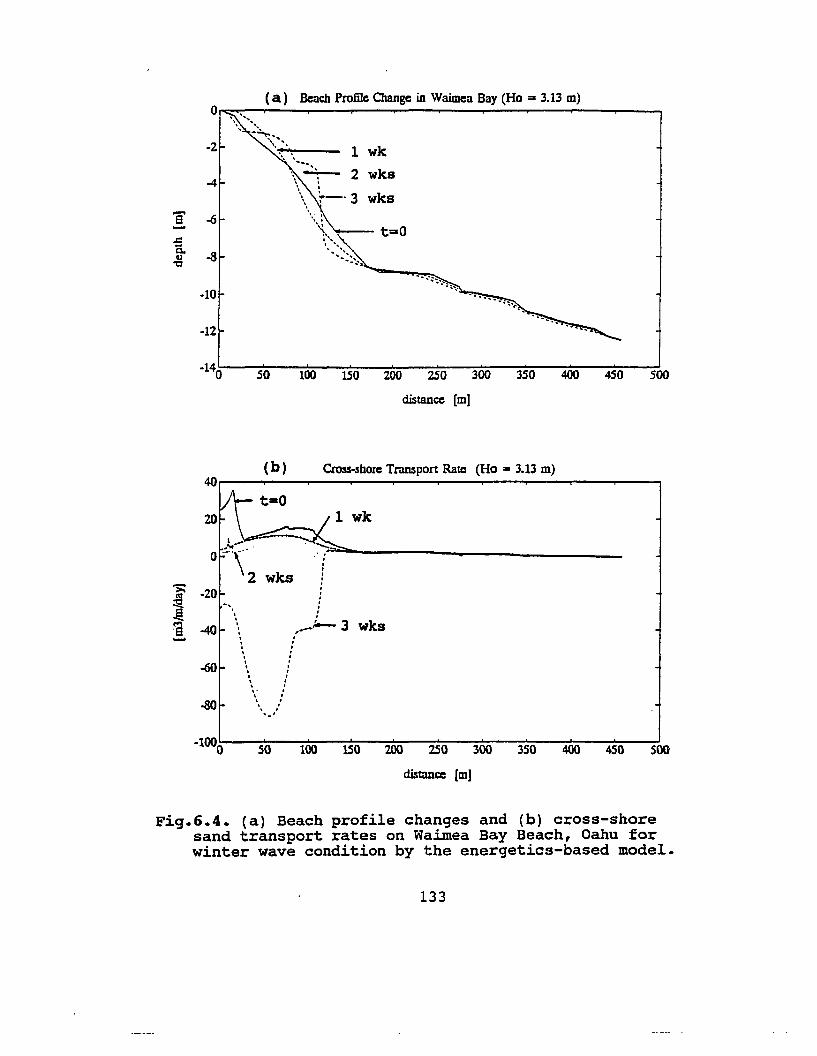
( a) Beach Profile Change in Waimea Bay(Ho =3.13 m)
'8-.cau'0
-2
-6
.........., ".. ~c-;
\.\ 1 wk.. ,.......\~ 2 wks, .... :"-'3 wks\\ .\~
\, t:30."\ ........<:~:~.
-10
-12
50 100 150 200 250 300 350 400 450 500
distance [m]
Cross-shore Transport Rate (Ho" 3.13 m)
-60
(b)4Or---.--....,...---.--........-=--..---~- .......---:.--,.------.J'r t-O
20-.!,.~ ~~Wk
0-\ ----------2 wks "f
'>: •<II -20 :
32. -"'. •~, i-'6 -40 \ ,_:-- 3 wks--- ~ l. ., .
\ :· .· .· .· .· ..' .. .. ." "'.'
so 100 150 200 250 300 350 400 450 500
distance [m]
Fig.6.4. (a) Beach profile changes and (b) cross-shoresand transport rates on Waimea Bay Beach, Oahu forwinter wave condition by the energetics-based model.
133

( a) Beach Profile Change in Waimea Bay (Ho =1.91 m)
-2
-4 taO' '....: ... 4 wks2 wks/"'<
-6 ':'.
-10
-12
50 100 150 200 250 300 350 400 450 500
distance [m)
4 wks
Cross-shore Transport Rate (Ho" 1.91 m)
wk
,·,,···--+-1- 2 wks:,I
·:.-- 3 wksII·:·,,··,,,·.......,)
5
0I:,
'>:-5
•~
,
.§. -10M
-,
8 J- -IS ',..,..,
-20 '" "..""".........
-25
50 100 150 200 250 300 350 400 450 500
distance [m)
Fig.6.5. (a) Beach profile changes and (b) cross-shoresand transport rates on Waimea Bay Beach, Oahu forsummer wave condition by the energetics-based model.
134

Gerritsen (1978) reported shoreline (MLLW) accretion by
about 17 m in the middle of Waimea Bay between January 11
and February 26, 1974. The volume change per unit width
above the MLLW reaches about 80 m3/m during the six weeks
(see Figure 6.2. Gerritsen, 1978). This accretion occurred
during the lowering phase of sea level.
Parker (1987) also measured the beach profile changes
above the shoreline between June 2, 1985 and January 23,
1986. She found the shoreline retreats by about 5 to 35 m
and the corresponding volume erosion per unit width was 10
to 35 m3/m at 5 transects during the 5 months (from summer
to winter). One transect connecting the Waimea River is
intentionally omitted in this study (see Figure 15 and 16,
Parker, 1987). Mean annual sea level cycle shows that the
sea level in June is about 3 cm lower than that in January
and 8 cm lower than that in September (maximum). That is,
the beach is submerged from June to September, and emerged
from September to January by the mean annual sea level
cycle. But summer wave conditions are calm, and winter wave
conditions are very intense as describ~d in CHAPTER 5.
Consequently, seasonal change of the beach profile may
be explained by the combined effects of annual sea level
cycle and wave condition rather than the annual change of
wave condition only.
135

6.2.2. Hapuna Beach, Hawaii
Hapuna Beach is located inside Kawaihae Bay on Hawaii's
west coast, a few miles south of Mauna Kea Beach. The beach
is straight and protected by rocky headlands on both ends
forming a littoral cell just like Waimea Bay Beach
(Fig.6.6). The beach is approximately 600 m long and 30 to
50 m wide in different seasons. The overall beach slope on
Hapuna Beach, Hawaii is fairly even (~ 1/20) and the
offshore area consists of rock and coral with numerous sand
pockets and some sand channels (Gerritsen, 1978). Due to
the gentle slope and finer sand ~ize of the beach, it seems
to endure large seasonal change, depending on the wave
climate with different seasons.
The shoreline of this beach was interpreted as "eroded"
by -9.14 m during about 38 years, which was from aerial
photos between March 1950 and May 1988. So the average rate
of shoreline change was converted to -0.24 m/yr (Makai Ocean
Eng., 1991). This value seems to be reasonably acccurate
since the mean sea level in March does not deviate much from
that in May (minimum le~el) when considering the mean annual
cycle. But if we may convert the shoreline position in May
1988 into that in March 1988, by adding the corresponding
horizontal distance (~ 40 cm) to the mean vertical sea-level
difference (~ 2 cm) between March and May from the beach
136

\
"io,r
"I
ii
r"
o 100 200M
Fig.6.6. Bapuna Beach: geography and bottom topography inthe nearshore region.
137

slope (= 1/20), then the shoreline recession rate could be
more accurately estimated. In other words, the retreat of
shoreline now becomes -9.54 m (= -9.14 m - 0.4 m) or the
average recession rate is -25 cm/yr between March 1950 and
1988. The linear trend of the RSL rise from the tide-gauge
records at Hilo, Hawaii (see Fig.2.1.(a» and the
correpsonding shoreline retreat by the Bruun Rule are +0.4
cm/yr and -8 cm/yr, respectively. Comparing this value with
the shoreline retreat by aerial photographs, The
contribution of the long-term effect of RSL rise by the
Bruun Rule is about 30% of the total retreat of the
shoreline. Then, the excessive rate of shoreline recession
or excessive retreat of shoreline must be explained by other
mechanics. That is, the shoreline retreat (R) based on the
Bruun Rule would be
R ===
S/tan P
4.0 [mm/yr] * 38 [yrs] * 20
3.04 [m]
The excessive retreat of shoreline during this period
becomes 6.10 m (= 9.54 m - 3.04 m), which may be associated
with the interannual or annual trends of sea- level rise and
the short-term events such as storm surges. The interannual
rising periods from the tide gauge records at Hilo, Hawaii
are as follows (Table 6.5):
138

Table 6.5. Interannual r~s~ng trends obtained from 12monthly running means of the monthly mean sea levelrecords at Hilo, Hawaii between 1955 to 1988.
============================================================period total rise rising rate
12.5 cm
10.0 cm
8 - 10 cm
11 - 15 cm
cm/yr3.40
2.75 - 3.75 cm/yr
1.14 - 1.43 cm/yr
6.25 cm/yr
3.33 cm/yr
cm8.5
1955 - 1958 (4 yrs)
1962 - 1968 (7 yrs)
1972 - 1973 (2 yrs)
1975 - 1977 (3 yrs)
1985 - 1988 (2.5 yrs)
vertical sea-level rise and corresponding retreat of
shoreline during each rising period is about 8 to 15 cm, and
1.6 to 3 m, respectively. Most of the rising trends match
with the occurrences of El Ninos: 1957-58, 1965, 1972-73,
1976, 1982-83, 1987-88. It is rather surprising that the
signal of 1982-83 El Nino, despite its strong intensity, is
not clear in the sea level records at Hilo. The sum of the
periods of interannual rising trends of sea level is 18.5
years or about 50% of the total period (from 1950 to 1988).
Although a falling trend follows a rising trend in the
interannual fluctuation pattern of sea level, some of the
transported sediments to the offshore region during the
rising period may not return to the onshore region during
the following falling period, signifying permanent beach
loss.
139
Because there is nearly no net longshore transport of
sediments in a littoral cell such as Hapuna Beach, Hawaii,
the excessive retreat of shoreline by about 6 m per 38 years
is predominantly due to the interannual sea-level
fluctuations, and possibly due to storm waves and currents.
Even in annual oscillation of cross-shore transports, some
of the sediments are permanently lost to the deep offshore
region (Campbell and Hwang, 1982).
Consequently, the impact of interannual rises of sea
level seems to be more significant than the effect of the
long-term linear rising trend in sea level.
Short-term erosion is basically due to wave actions,
that is, small onshore drift of Stokes flow above the trough
of the wave, offshore (return) flow below the wave trough,
and minor transport as bedload due to the combination of
gravity and friction.
The input parameters used in the energetic-based model
for short-term cross-shore sediment transport are basically
the same as in the case of Waimea Bay, Oahu, except the mean
sand diameter (~ 0.21 rom) and the corresponding fall speed.
For one transect in the middle of Hapuna Beach, Hawaii,
the beach-profile change and cross-shore sediment transport
rate are calculated with three different wave heights and
periods in deep water such that
140

(1) 50 = 2 m , T = 6 sec
(2) 50 = 2.5 m , T = 7 sec
(3) 50 = 3 m , T = 7 sec
The grid step for bottom profile is taken as 7.62 m, and the
time step is set as twice the average wave period.
In case (1), initial offshore transport rate is maximum
reaching up to 27 mJ/m/day at 25 m offshore, and greatly
reduced in a month (= 2 mJ/m/day) and even less thereafter.
In other words, most of the transport occurs within a week
as seen in Fig.6.7.(1). The depth of active profile change
is about 10 m, which seems to continuously erode during the
3 months (= 12 weeks).
In case (2), offshore sediment transport continues from
the initial condition until 2 weeks, when maximum offshore
transport occurs (up to 180 mJ/m/day) at 25 m offshore.
Then, the direction of the sediment transport is reversed at
the same 25 offshore region, where maximum onshore transport
rate is about 120 to 140 mJ/m/day, in 4 to 5 weeks. Due to
this onshore transport, the bottom is again accreted during
this period. The depth of active profile change becomes a
little deeper (= 12 m) than the case (1) (Fig.6.7.(2».
141

In case (3), maximum offshore transport occurs in a
week reaching up to 210 m3/m/day, which makes a small bar at
a depth of about 2 m. From the second week, overall erosion
occurs between shoreline and 190 m offshore (~ 13 m depth).
It is seen that the eroded material is accreted over deeper
region, especially between 270 m and 370 m offshore or the
depth range from 16 m and 26 m (Fig.6.7.(3».
Again, monthly rates of erosion and acretion from the
profile surveys during 1962-63 (Chamberlain, 1968) show a
smaller order of sand volumes than the model results in this
study (Table 6.6).
Table 6.6. Rates of erosion(-) and accretion(+) on (a)Waimea Bay, Oahu and on (b) Hapuna Beach, Hawaii.Data selected from Chamberlain (1968). Unit is in[m3/m/month] •
(a) Waimea Bay Beach, Oahu============================================================
5/62-7/62(2 mov )
-18.3
7/62-11/62(4 mo , )
- 7.4
11/62-3/63(4 mo.)
+ 9.3
3/63-5/63(2 mo , ]
-74.2
5/63-8/63(3 mo , )
+ 7.6
(b) Bapuna Beach, Hawaii============================================================
4/62-6/62(2 mo.)
- 3.4
6/62-9/62(3 mo.)
-11. 7
9/62-1/63(4 mo.)
- 0.5
142
1/63-4/63(3 mo , ]
- 6.9
4/63-7/63(3 mo , )
+20.6

Beach Profile Change in Hapuna Bay (Ho = 2 m)0
-5
-10
'8 -15-..cC. -201J'a
-25
·30
·350 50 100 150 200 250 300 350 400 450 500
distance em)
Cross-shore Transport Rate (Ho =2 m)
25
taO20
400 450 500350300250150 200
wks
8 wks
10050
distance (m]
( 1) 8 0 = 2 m, T = 6 sec
Fiq.6.7. Beach profile changes and cross-shore sandtransport rates for different wave conditions onHapuna Beach, Hawaii.
143

Beach Profile Change in Hapuna Bay (Ho:a 2.S m)0
-5
4-10 5
8'6
-15.......c:a. -20u"'Cl
-25
-30
-350 50 100 150 200 250 300 350 400 450 500
150
distance [m]
Cross-shore Transport Rate (Ho:ll 2.S m)
, .I :
-. 2 wks1oof-:( 3 wks
50 /lWk.... d ./t::lO0 _- ;.'yt;.~ ..--.-~! ':J..'J '/
-50f-
-100v5 wks
V 4 wks
50 100 150 200 250 300 350 400 450 500
distance [m]
(2 ) a, = 2.5 m, T = 7 sec
Fig.6.7. (continued) Beach profile changes and cross-shoresand transport rates for different wave conditions onHapuna Beach, Hawaii.
144

Beach Profile Change in Hapuoa Bay (Ho:::a 3 m)
-5
4-10
5
'8 -15 6-.=C. -20<U"0
-25
-30
-35 500
-1 wk- 2 wks
3 wks
- t=O
100 150 200 250 300 350 400 450 500
distance [m]
Cross-shon: Transport Rate (Ho. 3 m)
500450400300 350
t • 0
see 150 200 25050
-100
distance [m)
(3) Ho = 3 m, T ~ 7 sec
Fig.6.7. (continued) Beach profile changes and cross-shoresand transport rates for different wave conditions onHapuna Beach, Hawaii.
145

From the results of cross-shore transport rate and
bottom profile change for (a) winter and summer wave
conditions on Waimea Bay Beach, Oahu, and (b) 3 different
cases of wave height on Hapuna Beach, Hawaii, with the
energetic-based model, it can be said that:
'As the deep-water wave height increases, maximum
offshore transport occurs earlier and the offshore limit of
active profile change becomes deeper. The format:i.on of an
offshore bar seems to be an unstable transient stage to
adjust the equilibrium profile' •
146

6.3. BEACH RECOVERY
Beach processes basically show a three-dimensional
behavior which combines longshore and cross-shore processes.
Longshore sediment transports are generally carried by the
wave-induced longshore currents, which show maximum speed
near wave-breaking depth (Longuet-Higgins, 1972). In many
locations of the Hawaiian Islands wave breaking often occurs
a few times instead of once over the long reef bottoms,
i.e., highly dissipative and complex shallow bottoms
(Fig.6.8).
...... -- .......'--.~_oL)., _... . .
Fig.6.8. Schematic diagram of the complex wave-breakingprocess over the long reef bottom in the Hawaiian Islands.
147

Cross-shore sediment transports result from the
combined effect of onshore transport near the bottom due to
wave asymmetry and offshore transport below the wave trough
due to return flow, respectively. During storm-wave
conditions, the motion of sediments to the offshore
dominates due to strong return flow. Low and mild waves
cause sediments to move shorewards and often develop a berm
at the uprush level (Gerritsen and Jeon, 1991).
But, after a storm, subsequent mild waves recover the
beach only at shallow depths since the smaller wave heights
may not sufficiently affect the sediments at deeper depths
to which they were transported by the big storm waves. The
recovery processes is much slower than the erosion process.
Therefore, beach profiles, in general, never reach full
equilibrium state within a short time scale due to the
continuous variability of the wave-energy level.
Daily tidal motion may also contribute to beach erosion
and recovery (or accretion). The effect of beach erosion
by storm waves during HW (high water) may be significantly
larger than the case during LW (low water), if the tidal
difference is large. But the tidal difference in the
Hawaiian Islands is usually small (~ 60 cm) and hence the
contribution of daily tidal motion is insignificant relative
to that of big storm waves (> 5 m).
148

Model results show minor recovery only near the
foreshore region after deep erosion by model storm waves.
An arbitrary storm wave (He = 6 m, T = 12 sec) is exerted
for 36 hours on Waimea Bay Beach, Oahu and for 24 hours on
Hapuna Beach, Hawaii.
On Waimea Bay Beach, Oahu, overall erosion on the steep
shallow region (h = 0 to 8 m) and deposition on the gentle
deep region (h = 8 to 12 m) occurs for model storm waves (He
= 6 m). After 36 hours of the big waves, low wave height
(He = 1 m) is exerted for 60 hours. While there is no
active sediment transport below 5 m depth (= 100 m
horizontal distance from the shoreline), a,subsurface bar
forms at about 1 m depth and slowly migrates offshore
(Fig.6.9). The migration of the bar corresponds to the
maximum offshore transport rate around 50 m distance from
the shore after 1 day. On Hapuna Beach, Hawaii, a big storm
wave (He = 6 m) for 24 hours causes foreshore erosion and
forms a bar at 2 to 3 m depth, which results in accretion
down to 9 m depth. Contrary to Waimea Bay Beach, overall
deep erosion occurs down to a depth of about 20 m. The
recovery rate at shallow depths seems to be very slow even
for moderate wave conditions (He ~ 2 m) after the storm, due
to its steep slope (Fig.6.10).
Consequently, beach recovery by onshore sediment
transport in a short-time scale after big storm waves must
be carried out by non-breaking long waves.
149

Beach Recovery on Waimea Bay (Ho » 6 m -> 1 m)
60 brs
6 bra
after storm
500450400300 350250
original
20015010050
-8 -6-..c:Co
-8a.l't:l
-10
-12
-140
distance [m]
. Cross-shore Transport Rate on Waimea Bay (Ho ,. 1 m)
6 hrs
brs
i bra.@ -1 hra..., .8
;1, 36
- 60 hrs-1.5
-2hrs
~48 brs-2,5
-30 50 100 150 200 250 300 350 400 450 500
distance [m]
Fig.6.9. Beach profile changes and cross-shore transportrates under a small wave condition (50 = 1 m) after anarbitrary big storm (50 = 6m, t = 36 hours) on WaimeaBay Beach, Oahu.
150

Fig.6.10. Beach profile changes and cross-shore transportrates under a moderate wave condition (Ho = 2 m) afteran arbitrary big storm (Ho = 6 m, t = 24 hrs) on HapunaBeach, Hawaii.
151
-------_... - ._ .. _- ....._----_.-
Alternate onshore and offshore sediment transports
usually occur in an annual time scale, depending on
favorable (or mild) and unfavorable (or high) wave
conditions during different seasons. When favorable wave
conditions coincide with the lowering phase of the annual
cycle in sea level, beach recovery (or onshore transport)
rates may be faster. This implies that the rising phase of
sea level may result in more erosion or more offshore
transport of the eroded materials to greater depths when the
rising sea level coincides with unfavorable wave conditions.
In general, cross-shore sediment transport in an annual time
scale seems to occur alternately between summer and winter
seasons, and beach erosion and accretion (or recovery) rates
are comparable in the Hawaiian Islands. The seasonal
fluctuations in beach sand reservoirs for selected beaches
in the Hawaiian Islands during 1962 to 1963 (Moberly, 1968)
are shown in Fig.6.11.
In interannual and long-term scales, many of the
Hawaiian beaches do not totally recover. That is, they are
chronically losing sands to deep water. Moberly (1968)
argues about the mechanisms of sand loss to deep water on
the Hawaiian beaches -- 1) by waves and currents mainly
along sand-bottomed channels, 2) by sedimentation to deep
water, 3) by abrasion, 4) by cementation to beachrock, and
5) by storms. Although waves and currents are the primary
mechanism of littoral sand transports,
152

10 No 0'Beacllet
8 14
6-.f/J"'0>0- Z9. 4~U
It)
0--lJJ:E 20
=> 2....0>a: 8-0
1.0>a:lJJ .8(J)lJJa: .6
0 4Z« .4
fI) 1%
J:Co)«I.LJ .2CO
2 4 6 8 10 12 2 4 6 a 10 12
1962 1963
Fig.6.11. Seasonal fluctuations in beach sand reservoirsfor 86 selected beaches in the Hawaiian Islands during1962 to 1963 (after Moberly, 1968).
153
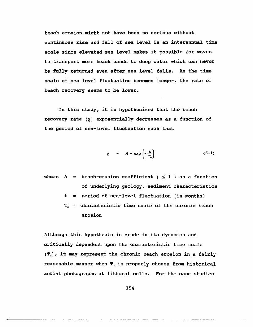
beach erosion might not have been so serious without
continuous rise and fall of sea level in an interannual time
scale since elevated sea level makes it possible for waves
to transport more beach sands to deep water which can never
be fully returned even after sea level falls. As the time
scale of sea level fluctuation becomes longer, the rate of
beach recovery seems to be lower.
In this study, it is hypothesized that the beach
recovery rate (X) exponentially decreases as a function of
the period of sea-level fluctuation such that
(6.1)
where A = beach-erosion coefficient ( < 1 ) as a function
of underlying geology, sediment characteristics
t = period of sea-level fluctuation (in months)
Tc = characteristic time scale of the chronic beach
erosion
Although this hypothesis is crude in its dynamics and
critically dependent upon the characteristic time scale
(Tc ) , it may represent the chronic beach erosion in a fairly
reasonable manner when Tc is properly chosen from historical
aerial photographs at littoral cells. For the case studies
154

at Waimea Bay Beach, Oahu, and at Hapuna Beach, Hawaii, Tc
was applied as 100 months (= 8.3 years), based on the aerial
photographs at the separate sandy beaches of the major four
Hawaiian Islands (Hwang, 1981; Makai Eng. & Ocean Eng.,
1991). This value is approximately twice the average ENSO
period.
Then, the beach recovery rate in annual oscillation
(t = 12 months) and in interannual fluctuation (t =4 years)
can be calculated as
and
Xlv r = exp (-..l£.) '" O. 89I 100
(6.2)
'" 0.62 (6.3)
It means that sediment losses by the sea-level fluctuation
with peri0ds of 1 year and 4 years are about 10% and 40%,
respectively. If we further assume that the sea-level
record at Honolulu can be applied to Waimea Bay Beach, Oahu
(which is fairly reasonable; see Fig.3.1) and the record at
Hilo to Hapuna Beach, Hawaii (which may be deviated a
little), then the net shoreline retreat by the sea-level
fluctuations with different time scales are calculated as follows:
155

(1) shoreline retreat = SLR * P(2) shoreline accretion = SLR * P * X
(1) - (2); net retreat = SLR * P * (1 - X)
where
SLR = vertical rise in sea level
p = beach-face slope
X = beach recovery rate
When applying long-term trend of sea-level rise, interannual
and annual fluctuations with beach recovery rates, the
contribution of each component to horizontal beach retreat
, can be estimated as in Table 6.7.
The contributions of long-term rise in relative sea
level is not significant at either beach; 4% at Waimea Bay
Beach, Oahu and 8% at Hapuna Beach, Hawaii. But, if global
warming is accelerating in the near future, thermal
expansion of seawater would contribute more to long-term
rise in relative sea level.
The effect of sea-level fluctuation on beach erosion
has not been studied as much as that of waves. But sea-
level fluctuation may cause significant beach erosion,
especially with an i.nterannual (or even longer) periods.
Annual oscillation of sea level as well as annual wave
climate are the primary cause of alternating cross-shore
156
..... _..._._- ---_._.- .._-... - . - .•......

sediment transport. However, the question of the portion of
sediment loss in annual onshore/offshore transport might not
have attracted the attention of most coastal geologists and
engineers probably because it could not be reasonably
measured, relative to the amplitude of annual oscillation.
The contributions of sea level changes (long-term rise,
interannual, and annual components) and waves (short-term)
to the shoreline retreat were estimated as about half and
half, respectively, at both beaches. The shoreline retreat
by sea-level change only can be formulated by
R ( t) • R1 ( t) + ~ ( t:) + ~ ( e)
• ;. e.[8+ 81 (1 -~exp (- ~:») + 52 (1 -Azexp (- ~:) )] (6.4)
where
R(t) = shoreline retreat
R1(t) = retreat by long-term sea-level rise
Rz(t) = retreat due to interannual sea-level fluctuation
R3(t) = retreat due to annual sea-level oscillation
5 =vertical sea-level rise
51 = mean height of the interannual fluctuation
52 = mean height of the annual oscillation
A1 = coefficient for the annual oscillation with time t 1
A2 = coefficient for the interannual fluctuation with
the quasi-period t 2
157

Table 6.7. Contributions of sea-level changes and waves toshoreline retreat at (I) Hapuna Beach, Hawaii, and at(2) Waimea Bay Beach, Oahu, based on the hypothesizedbeach recovery rate and measured aerial photographs.
(I) Hapuna Beach, Hawaii (P = IllS)
============================================================SLR
(vertical)E/A
(horizontal)Net
Retreat
long-term rise 0.4 cm/yr -0.06 m/yr -0.06 m/yr
interannual flue. 14 cm/4 yr -0.53 m/yr(3.5 cm/yr) +0.32 m/yr -0.21 m/yr
annual oscillation 10 cm/yr -1.50 m/yr+1.35 m/yr -0.15 m/yr
short-termeffects -0.37 m/yr
------------------------------------------------------------Total -0.79 m/yr
============================================================
(2) Waimea Bay Beach, Oahu (P = 1/20)
============================================================SLR
(vertical)E/A
(horizontal)Net
Retreat
long-term rise 0.2 cm/yr -0.04 m/yr -0.04 m/yr
interannual flue. 16.8 cm/4 yr -0.84 m/yr(4.2 cm/yr) +0.50 m/yr -0.34 m/yr
annual oscillation 9 cm/yr -1.80 m/yr+1.62 m/yr -0.18 m/yr
short-termeffects -0.39 m/yr
Total -0.95 m/yr============================================================
158

Here it is assumed that there is no longshore transport
and that the beach slope is always the same during the
erosion process. On the other hand, the irregularity of the
period (or the quasi-periodicity) of the interannual
fluctuation of sea levels makes it difficult to predict
beach erosion. When the (mean) period of ENSO events is
assumed as 4 years, the shoreline retreats at an isolated
beach with different slopes can be calculated as follows:
Table.6.8. Calculated shoreline retreats for differentbeach-face slopes with sea-level changes (S = 2 cm/10 yrs,S'= 10 cm/yr, S" = 16 cm/4yrs are assumed here.)
============================================================R1(t) R2(t) R](t) R(t)
P------------------------------------------------------------1:5 1.0 cm/yr 5.7 cm/yr 7.6 cm/yr 14.3 cm/yr1:6 1.2 6.8 9.1 17.11:7 1.4 7.9 10.7 20.01:8 1.6 9.0 12.2 22.81:10 2.0 11.3 15.2 28.51:20 4.0 22.6 30.5 57.11:30 6.0 33.9 45.7 85.61:40 8.0 45.2 61.0 114.21:50 10.0 56.5 76.2 142.71:75 15.0 84.8 114.3 214.11:100 20.0 113.0 152.4 285.4
============================================================
In addition, potentially accelerating global warming in
the near future will definitely cause the long-term effect
to contribute more to beach erosion.
159

CBAP!rER 7
COAS!rAL ZONE MAHAGEMEN!r
Human activities such as the building of ill-designed
coastal structures or sand mining, etc., may be significant
factors affecting coastal erosion in the Hawaiian Islands,
especially on Oahu and on Maui.
Harbor construction often requires dredging or widening
of a navigation channel, which may change natural sand
bypassing systems and groins or breakwaters may interupt the
transport of littoral material. These coastal structures
may change the patterns of wave propagation and energy
dissipation and cause serious leeside erosion.
Removal of beach material for nourishing other beaches
or for constructing structures and buildings, and mining of
subsurface sand resources may result in erosion by changing
the equilibrium profile. One serious reason for the chronic
erosion on Waimea Bay, Oahu is the sand mining which has
been carried out intermittently from 1949 to 1965 (Hwang,
1981).
Building seawalls, bulkheads, and revetments for
coastal protection may also cause erosion problems when they
are not properly constructed with consideration of all the
important design factors (Gerritsen and Jeon, 1991).
160

7 .1. AR~IFICIAL BEACR HOURISBMEe
Through natural nourishment beaches maintain a near
equilibrium state. Artificial nourishment as an alternative
could be applied to protect or to reduce beach erosion as
intermittant or continual processes. It is usually
economically attractive and environmently more acceptable.
There are some requirements for artificial nourishment
such that:
1) the grain size of nourished materials must be equal or
somewhat larger than that of original sands to prevent
the nourished beach from losing sands too fast;
2) nourished materials should not be calcified to avoid
formation of hard surfaces;
3) for recreational beaches, color should match the
original beach sands.
It seems worthwhile to discuss methods of artificial
nourishment although some of them are not directly related
to the natural beach systems.
follows:
They can be summarized as
1) direct placement by trucking and dredging,
2) dumping sands at one site (or stock-piling),
3) dumping sands at the shallow subsurface bottom (2 to 3 m)
161
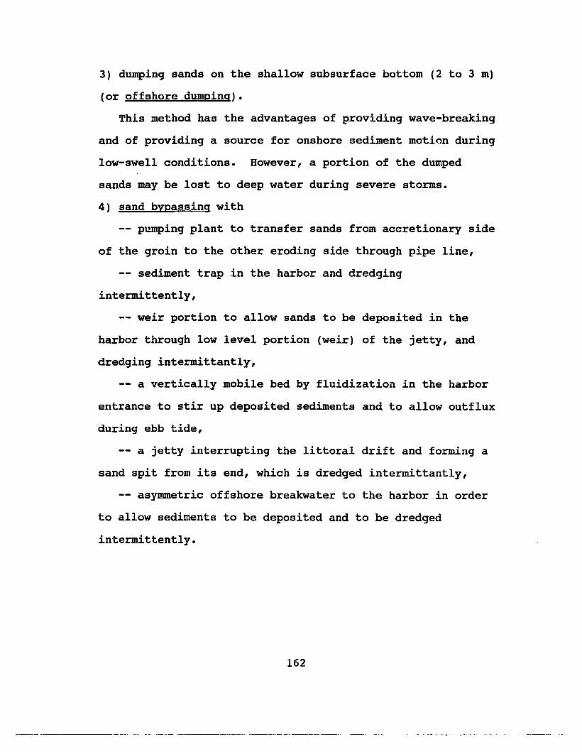
3) dumping sands on the shallow subsurface bottom (2 to 3 m)
(or offshore dumping).
This method has the advantages of providing wave-breaking
and of providing a source for onshore sediment motion during
low-swell conditions. However, a portion of the dumped
sands may be lost to deep water during severe storms.
4) sand bypassing with
-- pumping plant to transfer sands from accretionary side
of the groin to the other eroding side through pipe line,
-- sediment trap in the harbor and dredging
intermittently,
-- weir portion to allow sands to be deposited in the
harbor through low level portion (weir) of the jetty, and
dredging intermittantly,
-- a vertically mobile bed by fluidization in the harbor
entrance to stir up deposited sediments and to allow outflux
during ebb tide,
-- a jetty interrupting the littoral drift and forming a
sand spit from its end, which is dredged intermittantly,
-- asymmetric offshore breakwater to the harbor in order
to allow sediments to be deposited and to be dredged
intermittently.
162
------ --- -- "--- -- ---

7.2. BARD SOLUTIONS
Offshore breakwaters in shallow water parallel to shore
are frequently used as a hard solution against beach
erosion. Since they induce deformation of the shoreline due
to wave refraction and diffraction, the length of the
breakwater as related to the distance from the shoreline
must be carefully considered. Low-level or permeable
breakwaters may be used to prevent the formation of tombolo
: extreme shoreline deformation which causes the offshore
breakwater to be connected to the beach.
Groins to protect beaches from erosion may under
certain conditions be accepted such as when lee-side erosion
can be avoided or at least accepted. A groin constructed at
the boundary of a sandy beach and rocky shoreline will
usually not cause a beach-erosion problem. Where there is a
periodic reversal of longshore transports depending on the
direction of wave approaches, the fill between two groins
may oscillate from one end of the compartment to the other.
Multiple transitional groins with gradually reduced lengths
may be used in order to avoid an abrupt change between
protected and unprotected beach to reduce erosion of the
downdrift beach.
163

Revetment may be used to protect dunes from storm-tide
damage. There are two types of revetments:
1) Sloping revetments include
rubble mound
concrete blocks
placed stones, e.g., Kalama Beach (Maui),
Hilo Harbor (Hawaii)
asphalt concrete
stepped revetment.
2) Vertical types include
-- vertical gravity seawall, e.g., Mokuleia (Oahu); West
Maalaea Bay, Waimahaihai Beach, and Honokowai Beach (Maui)
steel bulkhead
concrete sheet piling
bulkhead with anchor.
A revetment is usually constructed (with toe protection)
considerably above MHW (mean high water), out of the normal
reach of the waves. In order to reduce the height of wave
runup on smooth slopes, ripples may be added. In case of
bulkhead revetment, the backside may be eroded by wave
overtopping during severe storms which may even form a
lagoon. Design factors are different from case to case. We
must consider all the important design factors
quantitatively in order to obtain suitable DWL (design water
level) and other design parameters for a certain case.
164

7.3. MAHAGEME~ STRATEGIES
Loss of beaches or coastal areas has both direct and
indirect consequences for coastal communities, requiring
abandonment and adjustment of property and, in extreme
cases, posing a danger to life (Carter, 1988). Basically
there are three kinds of coastal-zone-management strategies:
1) retreat •••• In accordance with rising sea level and
more disastrous coastal hazards by storm surges or tsunamis
in the future, all the residential areas are shifted inland
and a buffer system with natural or appropriate artificial
dunes, etc., is created. This strategy is most for
undeveloped coastal zones; regulations are the primary
management controls. It is different from a temporary
evacuation such as during a tsunami warning, in the sense
that a coastal buffer-zone is permanently preserved by legal
controls.
2) status quo with shore protection •••• For developed
coastal zones which endure erosion, coastal structures such
as breakwaters, revetments, or groins have been constructed
to protect further erosion. This method often causes
shoreline deformation and other erosion problems due to the
dynamic impact of the structures. It may be combined with
artificial nourishment.
165
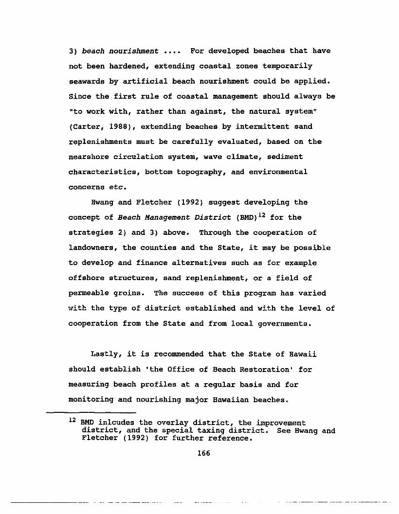
3) beach nourishment •••• For developed beaches that have
not been hardened, extending coastal zones temporarily
seawards by artificial beach nourishment could be applied.
Since the first rule of coastal management should always be
"to work with, rather than against, the natural system"
(Carter, 1988), extending beaches by intermittent sand
replenishments must be carefully evaluated, based on the
nearshore circulation system, wave climate, sediment
characteristics, bottom topography, and environmental
concerns etc.
Hwang and Fletcher (1992) suggest developing the
concept of Beach Management District (BMD)12 for the
strategies 2) and 3) above. Through the cooperation of
landowners, the counties and the State, it may be possible
to develop and finance alternatives such as for example
offshore structures, sand replenishment, or a field of
permeable groins. The success of this program has varied
with the type of district established and with the level of
cooperation from the State and from local governments.
Lastly, it is recommended that the State of Hawaii
should establish 'the Office of Beach Restoration' for
measuring beach profiles at a regular basis and for
monitoring and nourishing major Hawaiian beaches~
12 BMD inlcudes the overlay district, the improvementdistrict, and the special taxing district. See Hwang andFletcher (1992) for further reference.
166

CBAP'.rER 8
CONCLUSIONS
Long-term relative sea levels at selected island
stations in the North Pacific between the equator and about
30CN are examined in association with different time scales
of motions. Coastal response to these sea level dynamics
with different time scales are discussed in detail, based on
aerial photographs of shoreline changes. Wave climate
around the Hawaiian Islands as well as surf conditions on
Oahu are analyzed for simulating cross-shore beach erosion
processes with an energetics-based sediment transport model.
Tide-gauge records from the selected island stations in
the North Pacific (between the equator and 30CN) show the
following:
(1) The mean annual cycle of sea level is the strongest
signal at most of the stations, reaching about 10 em in the
mean annual height difference. The mean annual sea level
cycle and alternate annual wave conditions are the main
causes of the cross-shore oscillation of sediment transport,
with is some permanent loss of sediments to deep water.
167

(2) Long-term linear regressions show a trend of relative
sea level rise of +1 to +5 em/decade at most of the sea
level stations, primarily resulting from local tectonism
such as volcanic loading, plate movement with reef evolution
and subduction at the plate boundaries. Continual volcanic
loading at Kilauea, Hawaii results in consequential
subsidence of the Hawaiian Islands. Hence the Island of
Hawaii subsides with fastest rate (+ 2.5 mm/yr), the
neighboring island Maui with slower rate (+ 1.0 mm/yr), and
the Islands of Oahu (+0.15 mm/yr) and Kauai (+ 0.33 mm/yr)
with slowest rate. The slightly falling trend of sea level
at Midway. atoll (- 0.6 mm/yr) is associated with reef
evolution and plate movements. A secondary reason for the
rising sea level up to the present may be contributions from
the thermal expansion of sea surface waters by global
warming (+ 1.4 mm/yr). The rate of submergence is the sum
of the rate of subsidence and the global rate of sea-level
rise. It is likely thatin the future sea-level trend would
accelerate by the increasing rate of greenhouse gases into
the atmosphere up to 6 mm/yr. Although various GCMs
(general circulation models) have simulated present and
future atmosphere and oceans and support the accelerating
trend of sea level rise, there still exist a primary
uncertainty about the feedback mechanism of clouds before
transferring the "potentially increasing thermal energy" to
the ocean surface.
168
-----------

(3) Energy density distribution of monthly sea level
values shows a strong peak at about a four year period in
the Hawaiian Islands. A unique spectral peak with 25 to 30
year period is shown at Honolulu, Oahu, due to its
relatively longer time-series (> 85 years). Interannual
fluctuations from the time-series smoothed by twelve-month
running means show clear signals with periods between 2 and
7 years, which are closely associated with ENSO events. Sea
level rise and fall with an interannual time scale may be an
important factor for serious erosion problems, which seems
to affect beach erosion up to five to ten times the long
term linear trend. As the time scale of sea level
fluctuation becomes longer, beach erosion rate would be
higher (or beach recovery rate would be lower).
Reanalysis of previous aerial photographs of shoreline
changes in association with sea level fluctuations in the
Hawaiian Islands suggests the followings:
(4) Among the four major Hawaiian Islands (Hawaii, Maui,
Oahu, and Kauai), Maui seems to endure the most serious
problem of chronic beach erosion.
(5) In order to more precisely interpret long-term or
interannual shoreline changes from aerial photographs,
measurements must be carried out at least in the same month
169

of the year. This will remove the errors from different sea
levels on the annual cycle and from different wave
conditions in different months.
(6) Measurements at different times of the year may lead
to incorrect interpretations, even to reverse trends of
erosion/accretion of shoreline changes, unless the potential
errors included in aerial photographic measurements and
mapping procedures are systematically corrected.
(7) From aerial photographs it has been found that Waimea
Bay Beach on the north shore of Oahu has been seriously
eroded over the last decades; Bapuna Beach on the northwest
coast of Hawaii also eroded but to a lesser degree. The
primary reason for the erosion at Waimea Beach seems to be
the sand mining at Waimea Bay during 1949 to 1965.
Wave data analyses and an energetic-based cross-shore
sediment transport model give results as follows:
(8) Short-term change of beach profiles is basically
caused by wave conditions (wave height and period) in
addition to the effects of changes in MSL (mean sea level)
height.
170

(9) The average of significant wave height from NOAA buoy
(51001) during winter (December, January, and February)
exceeds 3 m and the average wave period is about 8 seconds,
while both wave height and period are greatly reduced during
summer (June, July, and August) (Ho = 2 m, T = 6 sec). This
is because relatively mild trade winds (northeasterlies)
prevail most of the year including summer and stronger North
Pacific swells (northwesterlies) control the wave climate in
winter.
(10) The surf conditions on the north and south shores of
Oahu are distinctly different; while the surf height on the
north shore is calm during summer and usually very high
during winter, it is fairly low on the south shore in both
seasons.
(11) Calculated beach profile changes at Waimea Bay Beach,
Oahu and on Hapuna Beach, Hawaii by a cross-shore sediment
transport model show similar patterns for different wave
conditions, except erosion to greater depth for higher wave
height. At Hapuna Beach, Hawaii, it is shown that higher
waves result in faster offshore transport and a greater
depth of the active zone.
(12) Beach recovery processes are usually much slower than
erosion processes, especially after big storm waves. Deep
171

erosion during storm waves can not be recovered by favorable
(or mild) waves of much longer duration. The erosion may be
partly recovered by non-breaking long waves such as 10n9
period swells, but eroded material may be permanently lost
to deep water.
Even in sea-level fluctuations at longer time scales
beach sediments cannot be fully recovered. As a hypothesis
it is proposed that the beach recovery rate exponentially
decreases as the period of sea-level fluctuation increases.
(13) The formation and migration of a bar at shallow
depths presents an unstable transient feature, which results
as the bottom tries to adjust to an equilibrium state during
a period of high waves. In this process standing
infragravity waves may play a role. Because of the time it
takes to reach equilibrium conditions and of the continuous
variability of the wave energy level and its directionality,
equilibrium conditions are hardly ever reached in the field.
172

APPBlIDICBS
A.I. DENSITY OF SEAWATER
The density of seawater is a function of temperature,
salinity and pressure: the parameters temperature and
salinity nonlinearly affect density, which increases by
approximately I kg m-3 for a change of temperature of
- SoC, for a change of salinity of + 1 psu (practical
salinity unit) or for a change of pressure of + 2,000 kPa.
In the open ocean, temperature ranges from - 2°e to
+ 30oe, salinity from 30 to 38 psu and sea pressure from 0
to about 105 kPa at a depth of 10,000 m. Salinity may fall
down to 0 near estuaries or melting ice. The density of
seawater at atmospheric pressure varies from about 1,000
kg m-3 for almost fresh water to about 1,028 kg m-3 for the
densest ocean water.
Thermal expansion coefficient correspondingly increases
as tempreature increases and hence volume expansion rate of
surface seawater at 31°e in the tropics is about 6 times
larger than that at O°C (Table A.I).
173

Table A.I. Temperature-dependency of the density ofstandard seawater (5 = 35 psu) at an atmosphericpressure (P = 0), and corresponding thermal expansioncoefficient (a), gradients of P and a with respect tosalinity (5).
============================================================P 5 T Gt "" a ap/a5 au/as
(bar) (psu") (OC) (kg m-3) ( 10-7K-1 )
------------------------------------------------------------0 35 -2 28.187 254 0.814 330 35 0 28.106 526 0.808 310 35 2 27.972 781 0.801 280 35 4 27.786 1021 0.796 260 35 7 27.419 1357 0.788 230 35 10 26.952 1668 0.781 200 35 13 26.394 1958 0.775 170 35 16 25.748 2230 0.769 150 35 19 25.022 2489 0.764 140 35 22 24.219 2734 0.760 120 35 25 23.343 2970 0.756 110 35 28 22.397 3196 0.752 90 35 31 21.384 3413 0.749 8
-----------------------------------------------------------* psu = practical salinity unit** G t = P (density) - 1,000 in [kg m-3
] .
174

A.2. MEAN ARNUAL TREND OF SHORELINE CHARGESIN THE HAWAIIAN ISLAHDS
Table A.2. Mean annual trend of shoreline changes Im/yr] on(a) Oahu (data from Hwang, 1981), (b) Hawaii, (c) Maui, and(d) Kauai (data from Makai Ocean Eng. and Sea Eng., 1991).(see also Fig.6.1)
(a) Oahu============================================================
North Windward South Leeward------------------------------------------------------------
0.22 1.12 -0.08 -0.07-0.01 0.08 -0.11 0.41
0.12 0.04 0.08 0.11-0.14 -0.23 0.10 0.31
0.68 0.07 0.04 0.130.0 -0.05 0.20 0.17
-0.94 -0.04 -0.17 0.120.01 0.31 -0.17 0.06
-0.03 -0.06 -0.16 -0.030.17 -0.11 0.08 -0.31
-0.01 -0.24 0.020.01 0.50
-0.24-0.09
(b) Hawaii============================================================
SA 0.06-0.03
0.16-0.09-0.24
0.14-0.16-0.24
0.00.130.02
HB 0.14-0.20-0.55-0.07
0.060.17
-0.020.160.08
-0.17-0.31-0.16-0.24-0.06
0.13-0.08-0.35-0.07
============================================================* (+); accretion, (-); erosion
175
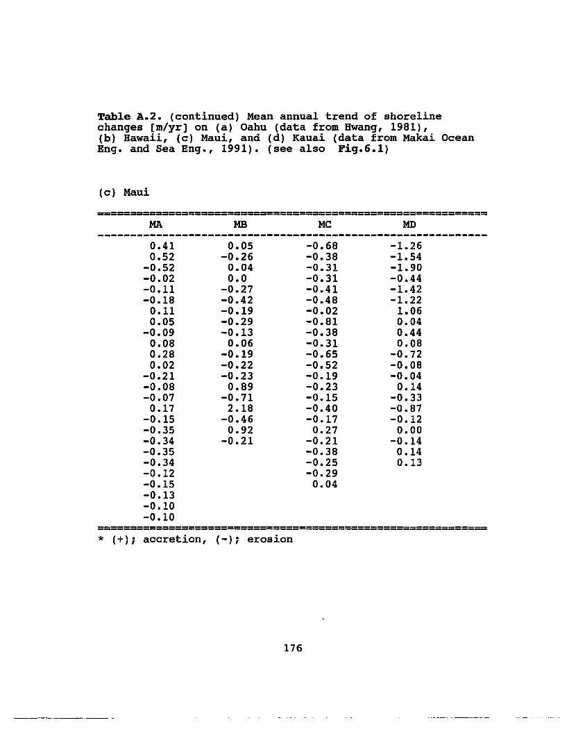
Table A.2. (continued) Mean annual trend of shorelinechanges [m/yr] on (a) Oahu (data from Hwang, 1981),(b) Hawaii, (c) Maui, and (d) Kauai (data from Makai OceanEng. and Sea Eng., 1991). (see also Fig.6.1)
(c) Maui
============================================================MA MB Me MD
0.41 0.05 -0.68 -1.260.52 -0.26 -0.38 -1.54
-0.52 0.04 -0.31 -1.90-0.02 0.0 -0.31 -0.44-0.11 -0.27 -0.41 -1.42-0.18 -0.42 -0.48 -1.22
0.11 -0.19 -0.02 1.060.05 -0.29 -0.81 0.04
-0.09 -0.13 -0.38 0.440.08 0.06 -0.31 0.080.28 -0.19 -0.65 -0.720.02 -0.22 -0.52 -0.08
-0.21 -0.23 -0.19 -0.04-0.08 0.89 -0.23 0.14-0.07 -0.71 -0.15 -0.33
0.17 2.18 -0.40 -0.87-0.15 -0.46 -0.17 -0.12-0.35 0.92 0.27 0.00-0.34 -0.21 -0.21 -0.14-0.35 -0.38 0.14-0.34 -0.25 0.13-0.12 -0.29-0.15 0.04-0.13-0.10-0.10
============================================================* (+); accretion, (-); erosion
176

Table Ao2. (continued) Mean annual trend of shorelinechanges [m/yr] on (a) Oahu (data from Hwang, 1981),(b) Hawaii, (c) Maui, and (d) Kauai (data from Makai OceanEng. and Sea Eng., 1991). (see also Fig.6.1)
(c) Kauai
============================================================KA
-0.14-0.34-0.37-0.13-0.63
0.690.720.300.260.170.17
KB
-0.19-0.18-0.15-0.21-0.15-0.09-0.10
0.100.15
KC
0.03-0.25
0.09-0.09
0.090.05
-0.35-0.50-0.08
0.460.00
-0.080.02
-0.05-0.06
0.120.240.32
-0.08-0.05
0.060.060.02
-0.15-0.07-0.17-0.10
0.320.62
-0.460.060.100.28
-0.17-0.23-0.35
KD
0.140.060.150.140.11
-0.210.090.311.090.020.280.12
-0.11
KE
0.16-0.05
0.03-0.02-0.16-0.14
0.10-0.33-0.04
0.16
KF
-0.200.160.670.09
-0.12-0.18
============================================================* (+); accretion, (-)i erosion
177
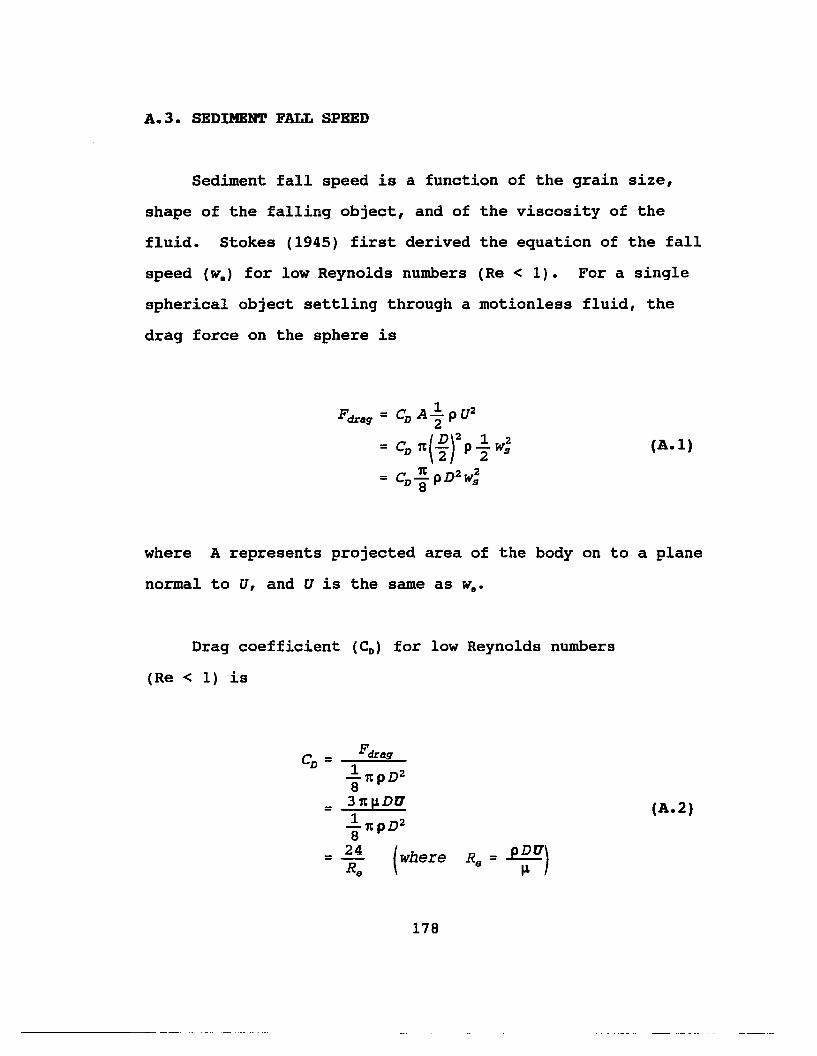
A.3. SEDIMENT FALL SPEED
Sediment fall speed is a function of the grain size,
shape of the falling object, and of the viscosity of the
fluid. Stokes (1945) first derived the equation of the fall
speed (w.) for low Reynolds numbers (Re < 1). For a single
spherical object settling through a motionless fluid, the
drag force on the sphere is
(A.1)
where A represents projected area of the body on to a plane
normal to U, and U is the same as w••
Drag coefficient (CD) for low Reynolds numbers
(Re < 1) is
Fdrag
..!.n pD2
8= 3nlLDU
..!.n pD2
8
= 24 (WhereRa
178
R = PDU)a lL
(A.2)

When the immersed weight (weight - buoyancy of the
fluid) is balanced by the drag force, the settling velocity
will be determined. The immersed weight (X) of a sphere is
(A.3)
Since Fdrag = X, we have
(A.4)
where dynamic viscosity v = ~/p. This is usually called the
'Stokes law'. The corresponding value of the Reynolds
number for a sphere falling down with the fall speed is
(A.5)
From a comparison of the observed and calculated fall
speeds of spheres of known size, Stokes law for the drag is
tolerably accurate for most purposes when Re < 1, and there
is no detectable error when Re < 0.5 (Batchelor, 1967).
179

Meanwhile, there have been several attempts to express
a sediment fall speed as a function of shape factor.as well
as size in a practical way. Maude and Whitmore (1958)
suggest that a sediment fall speed follows the relationship
such that
W = W (l-C)bS 0
where Wo is fall speed of a single grain, C is the
(A.6)
volumetric particle concentration, and b is a function of
particle size and shape. It was empirically obtained that
b = 4.65 for small particle and that b = 2.32 for large one.
Peirce and Williams (1966) have shown for four different
muds that the settling speed is proportional to (1 - C)5.
Hallermier's (1981b) empirical fitting for the fall speed of
common natural grains is consistent with the above results
(see Shore Protection Manual, 4-18, 4-21).
180

REFERENCES
Anders, F.J. and M.R. Byrnes (1991) Accuracy of shorelinechange rates as determined from maps and aerialphotographs. Shore and Beach, 58(2), 17-26.
Bagnold, R.A. (1966) An approach to the sediment transportproblem from general physics. u.S. Geological SurveyProf. Paper, 422-I.
Bailard, J. (1981) A simplified model for longshore sedimenttransport. Coastal Eng. Conr., 1444-1470.
Bailard, J. (1984) Simple model for surfzone sedimenttransport. Naval Civil Eng. Lab. Tech. Note,Port Hueneme, CA 93043.
Barnett, T.P. (1983) Recent changes in sea level and theirpossible causes. Climatic Change, 5(1), 16-37.
Barnett, T.P. (1984) The estimation of global sea levelchange: a problem of uniqueness. J. Geophys. Res., 89(C5), 7980-7988.
Barnett, T.P. (1988) Global sea-level change. In: Climatevariations over the past century and the greenhouseeffect: a report based on the first climate trendsworkshop, Washington D.C. National Climate ProgramOffice/NOAA, Rockville, Maryland, 7-9.
Barstow, S.F., H.E". Krogstad, K. Torsethaugen, and T.Audunson (1985) Procedures and problems associated withthe calibration of wave sensors, page 55-82, In:Evaluation, Comparison and Calibration of OceanographicInstruments. Graham & Trotman Ltd., London, pp267.
Barth, M.C. and J.G. Titus (1984) Greenhouse Effect and SeaLevel Rise. (Ed.) Van Nostrand Reinhold Co., New York,pp325.
Batchelor, G.K. (1967) An Introduction to Fluid Dynamics.Cambridge Univ. Press, London and New York.
Bodge, K.R. (1992) Representing equilibrium beach profileswith an exponential expression. J. Coastal Res., 8(1),47-55.
181

Braatz, B.V. and D.G. Aubrey (1987) Recent relativesea-level change in eastern north America.Soc. Ecen. Paleont. Mineral., 47, 29-46.
Broomfield, P. (1976) Fourier analysis of time series: andintroduction. New Yowk, John Wiley & Sons, 129-137.
Bruun, P. (1954) Coastal erosion and development of beachprofiles. u.S. Army Beach Erosion Board ofTech.Memorendum, .No.44, u.s. Army Corps of Engineers,Waterway Exp. Station, Vicksburg, Mississippi.
Bruun, P. (1962) Sea-level rise as a cause of shore erosion.J. Water. Barb. Div., Proc. of ASCE, 88(WW1), 117-130.
Bruun, P. (1988) The Bruun rule of erosion by sea-levelrise: a discussion on large-scale two- and threedimensional usages. J. Coastal Res., 4(4), 627-648.
Caldwell, P., K. Wyrtki, and S. Nakahara (1989) TOGA SeaLevel Center: Data from the Pacific. JIMAR contributionno.89-202, Univ. of Hawaii, pp34.
Campbell, J.F. (1972) Erosion and accretion of selectedHawaiian beaches, 1962-1972. HIG-72-20, The University ofHawaii Sea Grant Program, UNIHI-SEAGRANT-TR-72-02.
Campbell, J.F. and D.J. Hwang (1982) Beach Erosion at WaimeaBay, Oahu, Hawaii. Pac. Sci., 36, 35-43.
Carter, R.W.G. (1988) Coastal Environments -- AnIntroduction to the Physical, Ecological and CulturalSystems of Coastlines. Academic Press, London, pp617.
Chamberlain, T. (1968) The Littoral Sand Budget, HawaiianIslands. Pac. Sci., xxii, 161-183.
Coastal Engineering Research Center (1984) Shore ProtectionManual. (4th ed.), Dep. of the Army, u.S. Army Corps ofEngineers, Washington, D.C. 20314.
Dean, R.G. (1977) Equilbrium beach profiles: u.S. Atlanticand Gulf coasts. Department of Civil Eng., Tech. Rep.No.12, Univ. of Delaware, Newark, Delaware.
Dean, R.B. and E.N. Maurmeyer (1983) Models for beachprofile response. In: Komar, P.D. (ed.), CRC Handbook ofCoastal Processes and Erosion. CRC Press, Boca Raton,pp151-166.
Dean, R.G. (1991) Equlibrium beach profiles: characteristicsand applications. J. Coastal Res., 7(1), 53-84.
182

Douglas, B.C. (1991) Global sea level rise. J. Geophys.Res., 6981-6992.
Dubois, R.N. (1975) Support and refinement of the Bruun ruleon beach erosion. J. Geol., 83, 651-
Edelman, T. (1968) Dune erosion during storm conditions.Proc. Coastal Eng. (ASCE), New York, 719-
Emery, K.O. and D.G. Aubrey (1991) Sea Levels, Land Levels,and Tide Gauges. Springer-Verlag New York Inc., pp 237.
Fletcher, C.H. (1992) Sea-level trends and physicalconsequences: applications to the u.s. shore. EarthScience Review, 33, 73-109.
Folkert, M.B. and R.V. Woodle (1973) Status of environmentalsensing systems for unattended ocean buoys., 162-176, inEnvironmental Data Buoy Technology Workshop, Kingston.
Galvin: C.J. (1968) Breaker type classification on threelaboratory beaches. J. Geophys. Res. 73(12), 3651-3659.
Gerritsen, F. (1978) Beach and surf parameters in Hawaii.Sea Grant Tech. Rep. UNIHI-SEAGRANT-TR-78-02, Univ. ofHawaii, pp178.
Gerritsen, F. and D. Jeon (1991) Nearshore Processes andLittoral Drifts. (unpublished manuscript). Dept. OceanEng., Univ. of Hawaii, pp130.
Gill, A.E. (1982) Atmosphere-Ocean Dynamics. InternationalGeophys. Series, vol. 30, Academic Press, New York,pp662.
Gornitz, V., S. Lebedeff, and J. Hansen (1982) Global sealevel trend in the past century. Science, 215,1611-1614.
Gornitz, V. and S. Lebedeff (1987) Global sea-level changesduring the past century. Soc. Econ. Paleont. Mineral.,47, 3-16.
Graham, N.E., and W.B. White (1988) The EI Nino cycle: anatural oscillator of the Pacific ocean-atmospheresystem. Science, 240, 1293 - 1302.
Gray, W.M. (1979) Hurricanes: their formation, structure andlikely role in the tropical circulation. In: 'Meteorologyover the Tropical Oceans' (D.B. Shaw, ed.), pp151 - 218,Royal Meteor. Society, London.
183

Guilcher, A. (1988) Coral Reef Geomorphology. John Wiley &Sons Ltd., Chichester, pp228.
Guza, R.T. and E.G. Thornton (1981) Velocity moments in thesurf zone. Contract Rep. to Naval Civil Eng. Lab., pp56.
Hanson, H. and N.C. Kraus (1989) GENESIS: Generalized modelfor simulating shoreline change. Rep.l. Tech. Ref.,prepared for US Army Corps of Engineers, Washington, D.C.20314-1000.
Hayden, B., W. Felder, J. Fisher, D. Resio, L. Vincent, R.Dolan (1975) Systematic variations in inshore bathYmetry.Tech. Rep. No. 10, Dept. of Environmental Sci., Univ. ofVerginia, Charlottesville, Verginia.
Harvey, J.G. (1976) Atmosphere and Ocean: Our FluidEnvironments. 1st ed., Academic Press, pp143.
Hallermeier, R.J. (1981a) Seaward limit of significant sandtransport by waves: An annual zonation for seasonalprofiles. Coastal Eng. Tech. Aid No. 81-2, Coastal Eng.Res. Center, Vicksburg, Mississippi.
Hallermeier, R.J. (1981b) Terminal settling velocity ofcommonly occurring sand grains. Sedimentology, 28,
Holton, J.R. (1979) An Introduction to Dynamic Meteorology.2nd ed., Academic Press, pp391.
Hwang, D.J. (1981) Beach changes on Oahu as revealed byaerial photographs. HIG-81-3, Hawaii Inst. of Geophys.,Univ. of Hawaii.
Hwang, D.J. and C.H. Fletcher (1992) Beach management planwith beach management districts. Hawaii Coastal ZoneManagement Program, pp192.
Inman, D.L., W.R. GaYman, and D.C. Cox (1963) Littoralsedimentary processes on Kauai, a subtropical highisland. Pac. Sci., 17(1), 106-130.
Intergovernmental Panel on Climate Change (1990) ClimateChange: The IPCC Scientific Assessment. J.T.Houghton,G.T.Jenkins, and J.J.Ephraums (Ed.), Cambreidge Univ.Press.
Jenkins, G.M. and D.G. Watts (1968) Spectral Analysis andIts Applications. Holden-Day, Inc., San Francisco, pp525.
184
-~-----------
Jeon, D. (1990) Mean annual variations of the thermalstructure in the South China Sea. M.S. Thesis, Dept.Oceanography, Univ. of Hawaii, Honolulu, Hawaii 96822.
Kidson, C.(1986) Sea-level changes in the Holocene. p27-64In Sea-level Research: a manual for the collection andevaluation of data. O.v.d. Plasscbe (Ed.), Geo Books,Regency House, 34 Duke St., Norwich.
Kinsman, B. (1984) Wind Waves -- their generation andpropagation on the ocean surface, Dover Publ. Inc.,New York, pp676.
Komar, P.D. (1976) Beach Processes and Sedimentation.Prentice-Hall, Inc., New Jersey. pp429.
Komar, P.O. (1986) The 1982-83 El Nino and erosion on thecoast of Oregon. Shore and Beach, 3-12.
Komar, P.O. and D.B. Enfield (1987) Short-term sea-levelchanges and coastal ezosion. Soc. Econ. Paleont.Mineral., 47, 17-27.
Komar, P.O., N. Lanfredi, M. Baba, R.G. Dean, K.Dyer, T.Healy, A.C.Ibe, J.H.J. Terwindt, B.G. Thom (1991) Theresponse of beaches to sea-level changes: a review ofpredictive models. J. Coastal Res., 7(3), 895-921.
Kriebel, D.L. and R.G. Dean (1985) Numerical simulation oftime-dependent beach and dune erosion. Coast. Eng., 9,221-245.
Kriebel, D.L. and R.G. Dean (1993) Convolution method fortime-dependent beach-profile response. J. Water. P.Coast. Ocean Eng., 119(2), 204-226.
Laevastu, T., d.E. Avery, and D.C. Cox (1964) Coastalcurrents and sewage disposal in the Hawaiian Islands.HIG-64-1, Hawaii Inst. of Geophys., Univ. of Hawaii,pp101.
Lambeck, K. and S.M. Nakiboglu (1984) Recent global changesin sealevel. Geophys. Res. Letters, 11(10), 959-961.
Larson, M. (1991) Equilibrium profile of a beach withvarying grain size. Coastal Sediments '91 (ASCE),pp905-919.
Lisitzin, E. (1974) Sea-Level Changes. Elsevier Publ. Co.,Amsterdam, pp286.
185

Longuet-Higgins, M.S. (1972) Recent progress in the study oflongshore current. In: Waves in beaches and sedimenttransport, Academic Press, 203-248.
Madden, R.A. and V. Ramanathan (1980) Detecting climatechange due to increasing carbon dioxide. Sceince, 209,763-768.
Makai Ocean Eng., Inc. and Sea Eng., Inc. (1991) Aerialphotograph analysis of coastal erosion on the Islands ofKauai, Molokai, Lanai, Maui and Hawaii. Honolulu, Hawaii,pp200.
Maude, A.D. and R.L. Whitmore (1958) A generalized theory ofsedimentation. British J. Appl. Phys., 9, 477-482.
Moberly, R.J. (1968) Loss of Hawaiian Littoral Sand. J. Sed.Petrology, 38(1), 17-34.
Moberly, R.J., T. Chamberlain (1964) Hawaiian Beach Systems.HIG Rep. HIG-64-2, Hawaii Inst. of Geophys.,Univ. of Hawaii.
Moberly, R.J., D.C. Cox, T. Chamberlain, F.W.McCoy, Jr., andJ.F. Campbell (1963) Coastal Geology of Hawaii. HIG Rep.No 41., Hawaii Inst. of Geophys., Univ. of Hawaii, pp216.
Moberly, R.J., J.F. Campbell, and W.T.Coulbourn (1975)Offshore and other sand resources for Oahu, Hawaii. SeaGrant Tech. Rep. UNIHI-SEAGRANT-TR-75-03. also as HIG-7510, Hawaii Inst. of Geophys., Univ. of Hawaii, pp36.
Moberly, R.J. and F.T. Mackenzie (1985) Climate change andHawaii: significance and recommendations. HIG-S5-1,Hawaii Inst. of Geophys., Univ. of Hawaii, pp33.
Nakiboglu, S.M., K. Lambeck, and P. Aharon (1983)Postglacial sealevels in the Pacific: implications withrespect to deglaciation regime and local tectonics.Tectonophys., 91, 335-358.
Noda, E.K. and Associates, and DHM Inc. (1989) Hawaiishoreline erosion management study. Hawaii Coastal ZoneManagement Program, Office of State Planning.
Parker, S. (1987) Seasonal Changes in Beach Characteristicson the Island of Oahu, Hawaii. M.S. Thesis, Univ. ofHawaii, pp 122.
Patzert, W.C. (1969) Eddies in Hawaiian Waters. HIG-69-S,Hawaii Inst. of Geophysics, Univ. of Hawaii.
186

Peirce, T.J. and D.J.A. Williams (1966) Experiments oncertain aspects of sedimentation of estuary muds. Proc.Inst. Civil. Eng., 34, 391-402.
Peltier, W.R. and A.M. Tushingham (1989) Global sea levelrise and the greenhouse effect. Science, 244, 806-810.
Penland S. and K.E. Ramsey (1990) Relative sea-level rise inLouisiana and the Gulf of Mexico: 1908-1988. J. CoastalRes., 6(2), 323-342.
Pickard, G. and W.J. Emery (1982) Descriptive PhysicalOceanography -- An Introduction. (4th ed.) PergamonPress, pp249.
Pilkey, O.H., R.S. Young, S.R. Riggs, A.W. Sam Smith, H. Wu,and W.D. Pilkey (1993) The concept of shoreline profileof equilibrium: a critical review. J. Coastal Res., 9(1),255-278.
Pruszak, z. (1993) The analysis of beach profile changesusing Dean's method and empirical orthogonal functions.Coastal Eng., 19, 245-261.
Rayner, R.F. and S.J. Archer (1985) Evaluation andcalibration of oceanographic instruments -- the user'sview., 23-34, in Evaluation, Comparison and Calibrationof Oceanographic Instruments, vol. 4, Graham & TritmanLtd., pp267.
Roelvink, J.A. and M.J.F. Stive (1989) Bar-generating crossshore flow mechanisms on a beach. J. Geophys. Res.,94(C4), 4785-4800.
Schwartz, M.L. (1965) Laboratory study of sea-level rise asa cause of shore erosion. J. Geol., 73, 528-
Schwartz, M.L. (1967) The Bruun theory of sea-level rise asa cause of shore erosion. J. Geol., 75, 76-
Scott, G.A.J. and G.M. Rotondo (1983) A model for thedevelopment of types of atolls and volcanic islands onthe Pacific lithosphere plate. Atoll Res. Bull., 260,pp33. .
Shoshany, M. and A. Degani (1992) Shoreline detection bydigital image processing of aerial photography. J.Coastal Res., 8(1), 29-34.
Simpson, R.H., and H. Riehl (1980) The hurricane and itsImpact. Blackwell, Oxford.
187

Steetzel, H.J. (1990) Cross-shore transport during stormsurges. Proc. 22th Coastal Eng., 1922-1934.
Stokes, G.G. (1845) Trans. Camb. Phil. Soc., 8, 287.
Sturges, w. (1987) Large-scale coherence of sea level atvery low frequencies. J. Phys. Oceanogr., 17, 2084-2094.
Thieke, R.J. and R.J. Sobey (1990) Cross-shore wavetransformation and mean flow circulation. Elsevier Sci.Pub., Amsterdam, Coastal Eng., 14, 387-415.
Trupin, A., and J. Wahr (1990) Spectroscopic analysis globaltide gauge sea-level data. Geophys. J. International,100, 441-453.
Vellinga, A.P. (1986) Beach and dune erosion during stormsurges. Ph.D. thesis, Delft Univ. of Technology, Delft,The Netherlands.
Walker, J.R. (1974) Recreational Surf Parameter. Tech. Rep.,UH-Look Lab-73-30, Dept. Ocean Eng., Univ. of Hawaii.
Wang, N. (1993) Sediment transport and nearshorecirculation. Ph.D dissertation, Univ. of Hawaii.
Wigley, T.M.L. and S.C.B. Raper (1992) Implications forclimate and sea level of revised IPCC emission scenarios.Nature, 351, 293-300.
Wong, K.W. (1980) Basic mathematics of photogrammetry. In:C.C.Slama (ed.), Manual of Photogrammetry, 4th Ed.,American Soc. Photogr., Falls Church, VA, pp1056.
Woodworth, P.L. (1991) The permanent service for mean sealevel and the global sea level observing system. J.Coastal Res., 7(3), 699-710.
Wyrtki, K. and S. Nakahara (1984) Monthly maps of sea levelanomalies in the Pacific: 1975-1981. HIG-84-3, HawaiiInst. of Geophys., Univ. of Hawaii.
Wyrtki, K., B.J. Kilonsky, and S. Nakahara (1988) The IGOSSsea level pilot project in the Pacific. JIMARcontribution no. 88-0150, Univ. of Hawaii.
Wyrtki, K. (1990) Sea Level Rise: The Facts and the Future.Pac. Sci., 44(1), 1-16.
188