ISSN 0280-5316 ISRN LUTFD2/TFRT--5789--SE

Ultrasound-based Navigation for Mobile Robots

Jerker Nordh

Department of Automatic Control Lund University February 2007

Document name MASTER THESIS Date of issue February 2007

Department of Automatic Control Lund Institute of Technology Box 118 SE-221 00 Lund Sweden Document Number

ISRNLUTFD2/TFRT--5789--SE Supervisor Peter Alriksson and Karl-Erik Årzén at Automatic Control in Lund

Author(s) Jerker Nordh

Sponsoring organization

Title and subtitle Ultrasound-based Navigation for Mobile Robots (Ultraljudsnavigering för mobila robotar)

Abstract This thesis presents an implementation of a positioning and navigation system for a mobile robot using ultrasonic pulses and passive sensors that are part of a sensor network. The system uses the Telos Tmote Sky sensor-boards running Contiki. In addition to the Tmote Sky the mobile robot consists of a number of processors and is equipped with position encoders for the wheels in order to be able to accurately estimate the position using dead-reckoning. It is also equipped with an ultrasound transmitter. The sensor nodes are equipped with ultrasound receivers.

Keywords

Classification system and/or index terms (if any)

Supplementary bibliographical information ISSN and key title 0280-5316

ISBN

Language english

Number of pages 64

Security classification

Recipient’s notes

The report may be ordered from the Department of Automatic Control or borrowed through:University Library, Box 3, SE-221 00 Lund, Sweden Fax +46 46 222 42 43

Acknowledgments

I would like to thank professor Karl-Erik Årzén at the Department of Automatic Control in Lund for the opportunity to do this master thesis which has been very interesting and rewarding.

I would also like to Peter Alriksson for all the assistance when I encountered problems during my work and Rolf Braun for building the hardware required.

I also extend my thanks to Björn Grönvall at the Swedish Institute of Computer Science (SICS) for always being willing to answer questions regarding Contiki and the related software.

Jerker NordhLund, January 2007

5

Contents

1. Introduction................................................................................ 111.1 Background................................................................................................111.2 Purpose...................................................................................................... 12

2. Position estimation......................................................................142.1 Existing techniques....................................................................................142.2 Methods..................................................................................................... 152.3 Theory........................................................................................................172.4 Simulation..................................................................................................19

3. The Extended Kalman filter...................................................... 273.1 Introduction............................................................................................... 273.2 Model.........................................................................................................283.3 The Extended Kalman filter...................................................................... 29

4. Hardware.....................................................................................324.1 Tmote Sky..................................................................................................324.2 Mobile robot.............................................................................................. 334.3 Joystick...................................................................................................... 344.4 Sensor node...............................................................................................35

5. Software....................................................................................... 365.1 Contiki....................................................................................................... 365.2 I²C.............................................................................................................. 37

6. Distance measuring.....................................................................386.1 Theory........................................................................................................386.2 Implementation..........................................................................................396.3 Results....................................................................................................... 39

7. Wheel control.............................................................................. 417.1 Hardware................................................................................................... 417.2 Software.....................................................................................................417.3 Performance...............................................................................................43

8. Obstacle detection.......................................................................46

9. Robot controller..........................................................................489.1 Overview................................................................................................... 489.2 Design........................................................................................................489.3 Implementation..........................................................................................48

7

10. Multiple robots...........................................................................5010.1 Problem....................................................................................................5010.2 Solution....................................................................................................50

11. Implementation.......................................................................... 5311.1 Sensor nodes............................................................................................ 5311.2 Mobile robot............................................................................................ 5411.3 Radio packet types...................................................................................5911.4 I2C message types................................................................................... 61

12. Experimental results..................................................................63

13. Conclusion.................................................................................. 69

8

1. Introduction

This chapter gives the background to the master thesis, it's goal and limitations.

1.1 Background

RUNES is an European Union sponsored research project on the use of sensor networks, it stands for Reconfigurable Ubiquitous Network Embedded Sensors. The master thesis was done as a part of the Department of Automatic Control at LTH involvement in the RUNES[1] project.

RUNES consortiumThe following quote is from the RUNES consortiums introduction to the project, and summarizes their goals rather well.

“We stand on the brink of a revolution, in which the worlds of the embedded system and the Internet will collide. This will lead to the construction of the first truly pervasive networked computer systems and thus open up a marketplace of a

scale unparalleled in the history of technology. To realise this commercial potential requires a research and development programme focussed on the

creation of the infrastructure that actively promotes the efficient and inexpensive construction and anagement of novel services and applications that are

predictable and intuitively usable, so as to fulfil the global user expectations for invisible computing.”

Introduction to RUNES[2]

The RUNES consortium consists of 21 partners from 9 countries[3]:

• Australia: National ICT Australia, University of Queensland, Victoria University

• Canada: Communications Research Centre Canada• Germany: Industrieanlagen-Betriebsgesellschaft mbH, LiPPERT

Automationstechnik GmbH, Rheinisch-Westfaelische Technische Hochschule Aachen

• Greece: University of Patras• Italy: Politecnico di Milano, Università di Pisa• Hungary: Ericsson• Sweden: ConnectBlue AB, Ericsson AB, Swedish Institute of Computer

Science A, Kungliga Tekniska Högskolan, Lund Institute of Technology• United Kingdom: Kodak Ltd., Lancaster University, University College

London, United States of America, University of California, Berkeley, University of California, San Diego

9

RUNES project goalsThe RUNES project is scenario-based and all parties involved work together to solve a specific scenario[4]. The scenario chosen revolves around a road tunnel accident in central Europe. The idea is that in the future road tunnels will be equipped with sensor networks which can detect problems in the tunnel, i.e. fires. The scenario starts with an accident occurring in the tunnel, the sensors detects it and notifies the control center which can reroute the traffic around the tunnel.

During the rescue operation the sensor network will continuously assist the rescue personnel by keeping track of the temperature and other significant variables. The scenario also specifies that mobile robots will be sent into the tunnel to avoid sending humans into dangerous situations. In addition providing additional sensors the mobile robot should also be able to bridge gaps that might occur in the network if nodes are damaged for any reason.

To be able to accomplish these goals the project will have to develop middleware to hide the complexities of the sensor network from the applications, it must also allow the interconnectivity of different types of nodes that may be present both in the tunnel and on the vehicles that travel through it and on the personnel working in the tunnel.

To meet these requirements the project has chosen a component-based approach, where the different functionalities in the network are developed as components with well defined interfaces that can be dynamically loaded and unloaded. This facilitates the development of components independently of the rest of the system.

1.2 Purpose

The main focus of this thesis with regard to the RUNES-project is the part of the scenario that requires mobile robots moving within the network. This requires accurate positioning of the robot using the sensor network. The scenario also specifies that parts of the network shall become inoperable and that the mobile robot will move to these areas to reinforce the sensor network. This implies that the robot must be able to navigate with good precision even after it has lost contact with the network, implying the use of dead-reckoning during this part of the scenario. It must be able to correctly detect when it has reached the specified position and then communicate this back to the network control center which will attempt to reconfigure the network to work with the mobile robot as an additional node. If this fails the mobile robot should be able to resume operation and start moving between the segments of the network carrying network data with it.

The robot hardware already exists, so this thesis is limited to designing the software for the position estimation and navigation. In order to improve the robot handling the underlying control software for controlling the robot movements will also be improved.

Robot positioning and estimation have previously been implemented in a project course during the spring semester of 2006. This work will serve as a basis for this thesis, which will try to improve the performance and capabilities of the

10

implementation. This thesis will also use a more systematic approach to see what level of performance that can be expected.

11

2. Position estimation

This chapter discusses different techniques for determining the position of an object.

2.1 Existing techniques

CameraCamera-based system can, in combination with image processing, be used to detect and track the position of objects in an image. One such system is used in the thesis to check the accuracy of the position estimation implemented on the mobile robot.

GPSGPS is the Global Positioning System, it is a system consisting of more than two dozen satellites orbiting the earth. The system was developed by the United States Department of Defense and is controlled by the U.S. military.

Each satellite contains a very accurate clock and continuously broadcasts its current time as radio messages. Receivers can use the distance to a number of satellites to calculate its own position. The system gives a precision of roughly 15 m for civilian users, providing a somewhat more accurate signal to the U.S. Military. The GPS system does not work very well indoors and underground since it is difficult to receive the radio signals from the satellites under those conditions. If the signal has been reflected before reaching the receiver the precision is also degraded.

Ultrasound – CricketCricket[5] is a ultrasound based system for indoor localization developed at the Massachusetts Institute of Technology. It uses a combination of radio message and ultrasound pulses to measure the distance to a number of beacons.

The system is based around active beacons which transmits a radio message followed by an ultrasonic pulse. When the listener receives the radio message it tries to correlate it to the ultrasonic pulse and uses the difference in time of arrival to determine the distance. It is designed for use in indoor environments and gives a precision of 1-3 cm. Its main strength is that the listeners are entirely passive making it possible for the system to scale very well to a large number of listeners.

IMU – Inertial Measurement UnitAn IMU is a system used to track position and velocity, it typically consists of 3 accelerometers and 3 gyroscopes, each mounted in perpendicular directions. This provides the ability to measure acceleration and rotation in all directions. Often

12

the system also contains temperature sensors and/or is temperature controlled to increase the accuracy of the measurements. By accumulating this data it is possible to calculate the position, however due to measurement errors this leads to drift in the estimates, requiring the system to be reset according to a external reference regularly.

2.2 Methods

This section briefly discusses different methods for determining the position of an object

TriangulationThe method of measuring the angle to a given object from at least two known reference positions to determine its position is known as triangulation[6] . To determine a position in a three dimensional space at least two reference positions are required. The use of triangulation requires the ability to measure the angle between the object and reference points.

TrilaterationTrilateration[7] uses distances to a number of known reference points to determine the position. To determine a point uniquely in a two-dimensional plane at least 3 distances are required, in a three-dimensional space 4 measurements are required. Trilateration needs the ability to accurately measure the distance to the object from different reference points.

MultilaterationMultilateration[8] is a method for using the difference in time of arrival of a signal to different receivers, the main difference to trilateration is that it does not need to know the time at which the signal was transmitted. To determine the position of an object in a three dimensional space at least 4 such receivers would be required. Multilateration is dependent on the ability to accurately measure the time difference of arrival for signals.

The Kalman filterThe Kalman filter is a method for combining the use of measurements affected by noise with a model for how the object is assumed to be moving. The Kalman filter could be implemented using any of the above methods for estimating the position.

The Kalman filter also uses the inputs of the model to predict the behavior, in this case the available inputs are the velocity estimates for the two wheels.

The Extended Kalman filterThe Kalman filter requires a linear relationship between the measurement

input and the model states, but it is also possible to use a so called Extended Kalman filter which allows the use of non-linear relationships. This also makes it possible to use a non-linear model for how the object is assumed to move.

13

Basically the Extended Kalman filter takes a non-linear model and linearizes it around the current estimate, and then works in the same way as the Kalman filter.

Using an Extended Kalman filter it is also possible to use any measurements that can be estimated from the current model, that is the as long as the measured quantity is somehow related to the position the Extended Kalman filter can use it to improve the estimation of the position. This has the advantage that the relative accuracy of each measurement can also be taken into consideration when updating the estimate.

Method selectionBecause of the available hardware the positioning has to be done using ultrasound pulses. Since the nodes have no ability to decide from which direction the pulse arrived, the possibility of using triangulation is ruled out. This leaves the possibility of using multilateration, or estimating the distance and using that for either trilateration or as inputs to an Extended Kalman filter.

The main advantage of multilateration is that there is no need to know when the signal was emitted, but since the nodes clocks are not synchronized we would first have to synchronize them, eliminating this advantage.

If a radio package is sent at the same time as the ultrasound pulse it is possible to use the difference in time of arrival of the two signals to calculate the distance to each node, assuming that the propagation velocity of the radio signal is much larger than that of the signal. This gives an accurate way of calculating the distance. The distance can then be used either for trilateration or directly as input to the Extended Kalman filter.

Of these methods the trilateration and the use of distance measurements to the Extended Kalman filter were selected for evaluation by simulation in Matlab.

14

2.3 Theory

Trilateration

The distance measurement to each reference point will form a sphere of possible positions. Assuming that P1,P2 and P3 all lie in the same plane and that P1 is at the origin and P2 is on the x-axis, it can easily be shown that the point of intersection is

x=r1

2−r22d 2

2d

y=r 1

2−r3x−i 2

2j

j2−r 1

2−r 22d 22

8 d 2 jz=r1

2−x2− y2

The sign of the z coordinate cannot be uniquely established without a fourth measurement. For the purposes of this report it is, however, assumed that the positive solution is the correct one. The conditions above can easily be fulfilled for any three points by a simple linear transformation, as long as they are not on the same line.

First the coordinates of P1 are subtracted from each of the other points to fulfill the requirement that P1 must be at the origin. The other requirement is that P2 must lie on the x-axis, this is accomplish by making a coordinate system

15

r1 r2

r3

d

i

j

x

y

P1 P2

P3

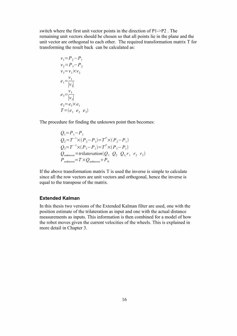
switch where the first unit vector points in the direction of P1->P2 . The remaining unit vectors should be chosen so that all points lie in the plane and the unit vector are orthogonal to each other. The required transformation matrix T for transforming the result back can be calculated as:

v1=P2−P1

v2=P3−P2

v3=v1×v2

e1=v1

∣v1∣

e3=v3

∣v3∣e2=e3×e1

T=e1 e2 e3

The procedure for finding the unknown point then becomes:

Q1=P1−P1

Q2=T−1×P2−P1=T T×P2−P1Q3=T−1×P3−P1=T T×P3−P1Qunknown=trilaterationQ1 Q2 Q3, r 1 r2 r3Punknown=T ×QunknownP0

If the above transformation matrix T is used the inverse is simple to calculate since all the row vectors are unit vectors and orthogonal, hence the inverse is equal to the transpose of the matrix.

Extended KalmanIn this thesis two versions of the Extended Kalman filter are used, one with the position estimate of the trilateration as input and one with the actual distance measurements as inputs. This information is then combined for a model of how the robot moves given the current velocities of the wheels. This is explained in more detail in Chapter 3.

16

2.4 Simulation

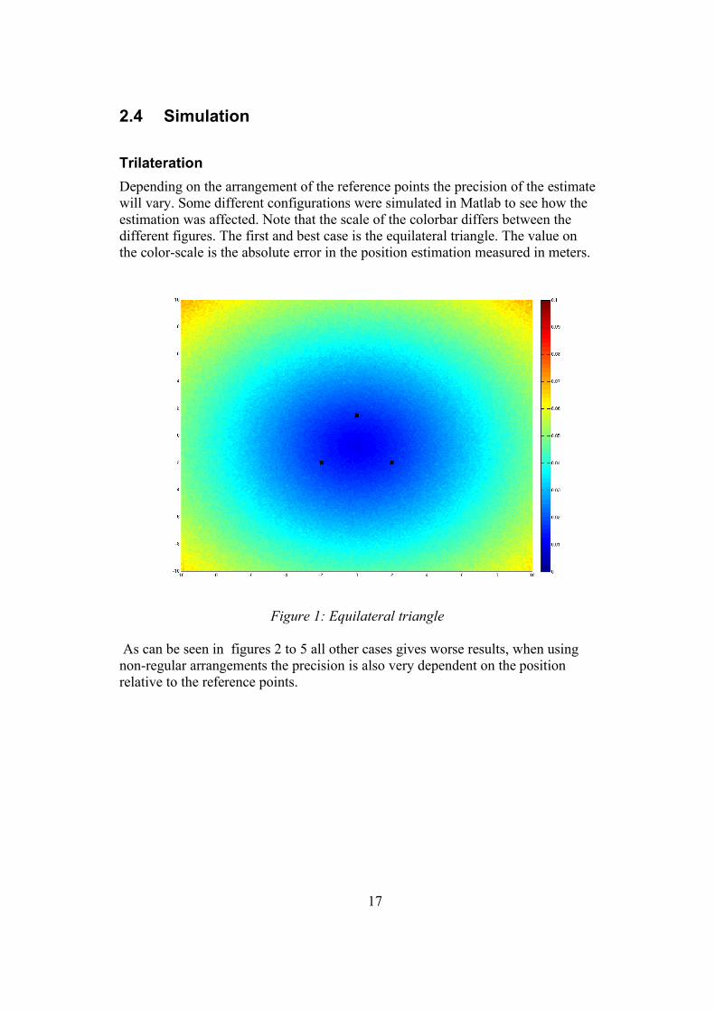
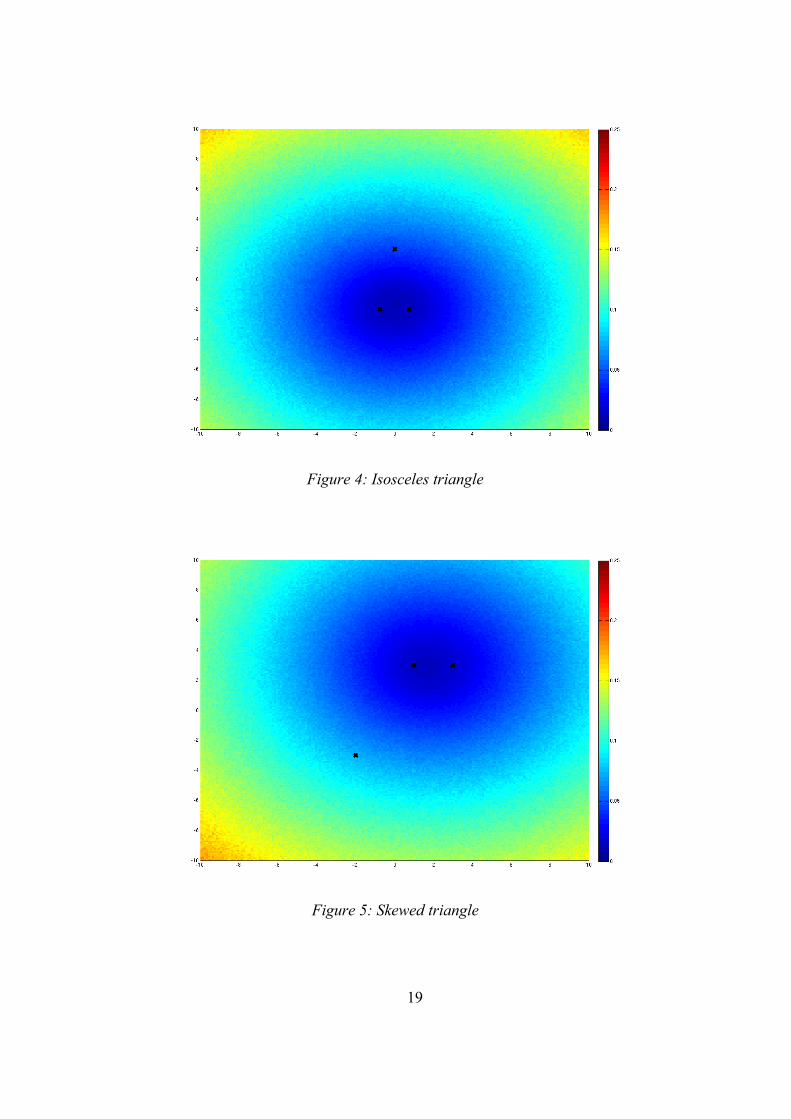
TrilaterationDepending on the arrangement of the reference points the precision of the estimate will vary. Some different configurations were simulated in Matlab to see how the estimation was affected. Note that the scale of the colorbar differs between the different figures. The first and best case is the equilateral triangle. The value on the color-scale is the absolute error in the position estimation measured in meters.

As can be seen in figures 2 to 5 all other cases gives worse results, when using non-regular arrangements the precision is also very dependent on the position relative to the reference points.

17

Figure 1: Equilateral triangle

18

Figure 2: Low triangle

Figure 3: Narrow triangle

19

Figure 5: Skewed triangle

Figure 4: Isosceles triangle

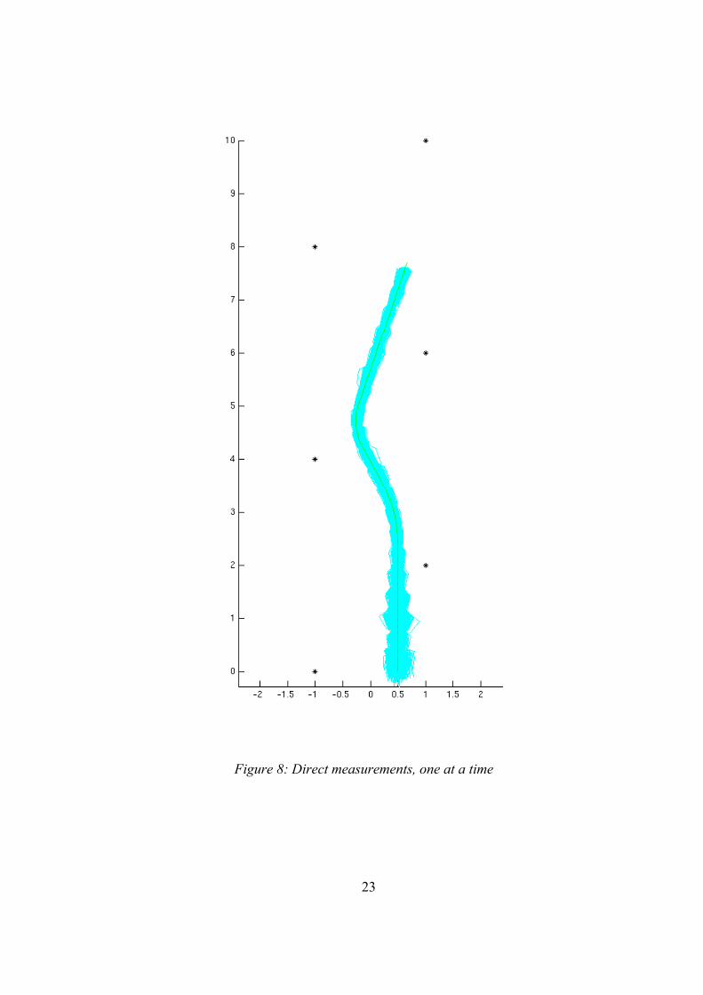
Extended Kalman filterWhen simulating the Extended Kalman filter the model for how the mobile robot moves was used to generate a reference trajectory with the wheel velocities as inputs, this trajectory was then used to generate noise-corrupted range measurements to each reference point. The Extended Kalman filter was then used to estimate the position using just the noise-corrupted input signals and range measurements. The noise added was normally distributed with standard deviation comparable to what was observed in the physical process.

Four different methods were simulated. The first uses one using trilateration to estimate the position which is then used as an input. The other three methods all use the range measurements directly, but differ in how many measurements that are handled at a time. One uses all measurements at the same time, one uses a single measurement at a time, and the third uses two measurements at a time. If the total number of available measurements is odd a single measurement is used at the end. The reason for not using all measurements at the same time is that the implementation requires the inversion of a matrix with the same dimensions as the number of measurement, which can be very computationally expensive when there are many measurements.

As can be seen in figures 6 to 9 all the methods give approximately the same results. However, one important distinction between the trilateration and the direct methods is not visible in this test; when the positioning of the reference nodes is poor the direct methods will take that into consideration and thus rely more on the model and less on the measurements. Since the robot is expected to be able to navigate when regions of the sensor network may be inoperable the direct methods are much better suited for the implementation. The difference between the direct methods are hardly discernible, thus there is no reason to not choose the method which uses one measurement at a time since it is vastly less computationally expensive than the others.

Figure 6 to 9 show the estimated paths from a number of simulations with the correct path superimposed as a green curve.

20

21

Figure 6: Trilateration

22

Figure 7: Direct measurements, all at once

23

Figure 8: Direct measurements, one at a time

24

Figure 9: Direct measurements, two at a time

3. The Extended Kalman filter

3.1 Introduction

A Kalman filter is a method for combining noisy measurements of a process with a model of how the process works. The inputs to a Kalman filter are the measurements, the process model, the model noise and the measurement noise. The noise describes the error in the measurements and model. For linear systems it is possible to calculate an optimal estimation strategy for the process state given these inputs. Both the model noise and measurement noise are assumed to be zero mean multivariate normally distributed.

The Extended Kalman filter is an extension of the Kalman filter for non-linear systems. This is achieved by linearizing the system for each iteration. Unlike the standard Kalman filter the Extended Kalman filter can not be guaranteed to be optimal, nor that it will converge to the correct solution.

Due to the difficulties in determining the noise of the model for the mobile robot the noise matrices have been experimentally determined to give a reasonable trade off between how fast the estimate converges and how much noise is present in the estimate.

In addition to estimating the state the Kalman filter also estimates the covariance of the estimated states, this is used for determining the relation between the state variables and to estimate how good the current estimate is.

25

3.2 Model

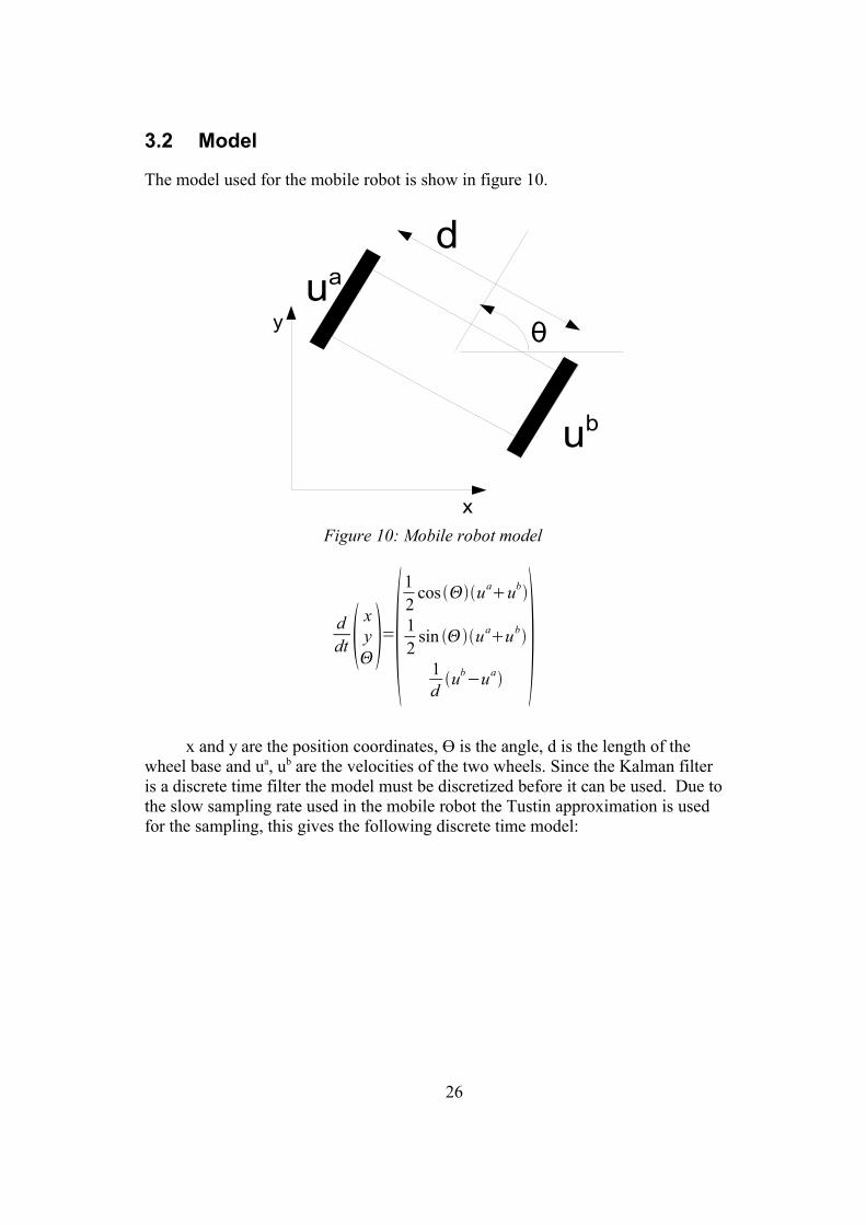
The model used for the mobile robot is show in figure 10.

ddt x

y=

12

cos uaub

12

sin uaub

1dub−ua

x and y are the position coordinates, Ө is the angle, d is the length of the wheel base and ua, ub are the velocities of the two wheels. Since the Kalman filter is a discrete time filter the model must be discretized before it can be used. Due to the slow sampling rate used in the mobile robot the Tustin approximation is used for the sampling, this gives the following discrete time model:

26

Figure 10: Mobile robot model

d

x

y

ub

ua

θ

ddt

≈2 z−1h z1

xyk

= f ⋅=x k−1h4cos k−1u

ak−1ub

k−1cosk ua

kubk

yk−1h4sink −1u

ak−1ub

k−1sin k ua

kubk

k−1h2d

uak−1−ub

k−1uakub

k

The function f() is the so called next-state function, which calculates the next state using the current state and the inputs. When using the Tustin approximation the state at time k is dependent on the input a time k and k-1. This often this results in that numerical methods have to be used when calculating the next state. However in this case the relationship between the state variables allows an analytical solution since the Ө-state is independent of both x and y and x and y are independent of each other.

3.3 The Extended Kalman filter

The Extended Kalman[9] filter needs two models, the state transition model and the observation model. These two models relate the current state to the next state and to the external measurements. The state transition model must be a differentiable function of the previous state and the current input and current model noise (wk) . The observation must be a differentiable function of the current state and measurement noise (vk). wk has the covariance Qk and vk has the covariance Rk. This can be written as:

xk= f xk−1 , uk ,w k z k=h xk , v l

The function f is the same as the next-state function in the discrete time model in Section 3.2. The function h() is dependent on whether trilateration or direct measurements are used. For trilateration it becomes:

zk x=x k x

z k y=x k y

When using direct measurements the observation model becomes slightly more complex, for each distance measurement, ri to the point Pi, the following model is used (time index k omitted for clarity):

z i=P ix−x 2P iy− y2P iz−z 2

27

The filter consists of two phases, the predict phase and the update phase. For every time step the next state is predicted during the predict phase. Since measurements may not be available at all time steps the update part of the filter is only used during those time steps where new measurements are available.

When updating the covariance the non-linear function f() and h() cannot be used directly, instead the Jacobian's Fk and Hk, of f() and h() respectively, are used. Since they are matrices of the partial derivatives they must be recalculated at each time-step using the current state.

Predict phaseThe predict phase uses the non-linear state transition model and predicts the next state and updates the covariance matrix of the state estimate.

xk= f xk−1 , uk P k∣k−1=F k P k−1∣k−1 FT

kQ k

Update phaseThe update phase takes the current state and estimates what the measurements should be using the observation model. The result is then compared to the actual measurements, and the current state is corrected accordingly taking the measurement noise into consideration.

yk=zk−h xk∣k−1,0Sk=H k P k∣k−1 HT

kRk

K k=Pk∣k−1 H Tk S−1

k

xk∣k=xk∣k−1K k yk

P k∣k= I−K k H k Pk∣k−1

ImplementationThe implementation of the Kalman filter is computationally expensive. To increase efficiency results of expensive trigonometric functions are cached. No matrix math library is used, so all matrix operation are expanded manually, this also provides the possibility for further optimizations by manually removing multiplications by constant zeros and ones. Below the update function is shown as an example.

28

/* Predict next position, Tustin approximation */void kalman_predict(float X[3], float P[3][3],

float u[2], float uo[2]) { /* old theta */ float tho = X[2];

/* Predict new theta using tustin */ float th = X[2] + H_KALMAN/(2.0f*L_BOT)* ((u[1]-u[0]) + (uo[1]-uo[0]));

/* Store computed trig funcs, saves approx 70 ms/call */ float cos_th = cosf(th); float sin_th = sinf(th); float cos_tho = cosf(tho); float sin_tho = sinf(tho);

/* store computed values to save time (saves approx 7 ms/call) */ float u_cos_th = (u[0]+u[1])*cos_th+(uo[0]+uo[1])*cos_tho; float u_sin_th = (u[0]+u[1])*sin_th+(uo[0]+uo[1])*sin_tho;

X[0] = X[0] + H_KALMAN/4.0f * u_cos_th; X[1] = X[1] + H_KALMAN/4.0f * u_sin_th; X[2] = th;

float h1 = -H_KALMAN/4.0f * u_sin_th; float h2 = H_KALMAN/4.0f * u_cos_th;

float a = P[0][0]; float b = P[1][1]; float c = P[2][2]; float d = P[1][2]; float e = P[0][1]; float f = P[0][2];

float fh1c = f+h1*c; float dh2c = d+h2*c;

/* P = Fk*P*Fk+Qk' */ P[0][0] = (a+h1*f)+fh1c*h1+QK11; P[0][1] = (e+h1*d)+fh1c*h2+QK12; P[0][2] = fh1c+QK13;

P[1][0] = (e+h2*f)+dh2c*h1+QK21; P[1][1] = (b+h2*d)+dh2c*h2+QK22; P[1][2] = dh2c+QK23;

P[2][0] = fh1c+QK31; P[2][1] = dh2c+QK32; P[2][2] = c+QK33; return;}

29

4. Hardware

The system consists of a number of sensor nodes with ultrasound receivers and a mobile robot with an ultrasound transmitter. Both the nodes and the robot use the Tmote Sky hardware as the interface to the network.

4.1 Tmote Sky

The Tmote Sky is a wireless sensor network platform manufactured by the Moteiv corporation[10]. Its main features are:

• 250kbps 2.4GHz IEEE 802.15.4 Chipcon Wireless Transceiver • 8MHz Texas Instruments MSP430 micro controller • USB interface

The version used in the thesis has been mounted in a custom enclosure built at the Department of Automatic Control at Lund Institute of Technology. A Telos Mote board is shown in figure 11.

30

Figure 11: Telos Mote

4.2 Mobile robot

There are two mobile robots used in the thesis, they have the same overall design with some minor differences. One of the robots is shown in figure 12.

The robots are of dual-drive unicycle type, they have two independently driven wheels, and uses a third ball-type wheel that is free to rotate in all directions to maintain balance. Each motor is controlled by one Atmel AVR Mega16 processor. The two sides are entirely identical, this results in the directions for the right and the left side being reversed, so for the robot to move forward one side has to run in the positive direction and the other side in the negative direction.

The robots are also equipped with an ultrasound transmitter which is connected to an additional AVR Mega16 processor. A plastic cone has been mounted directly above the ultrasound transmitter in order to scatter the sound in a 360 º plane. Each robot also has a Tmote Sky which provides the connection to the sensor network over the radio interface. The Tmote Sky also acts as master of the I²C-bus which all processors are connected to. A schematic overview of the hardware is shown in figure 13.

One of the robots have additional hardware in order to detect and avoid collisions. It consists of two touch sensor and an IR-distance sensor mounted on a RC-servo. The RC-servo can be used to sweep the distance sensor in an arc in front of the robot, thus acting as a form of IR-radar that can be used to detect obstacles. All of these sensors are connected to same processor that controls the ultrasound transmitter.

31

Figure 12: RBBot mobile robot

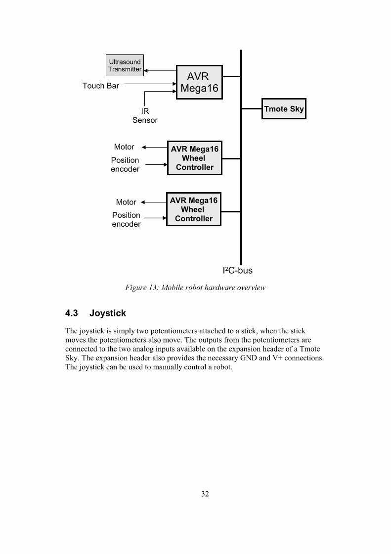
Figure 13: Mobile robot hardware overview

4.3 Joystick

The joystick is simply two potentiometers attached to a stick, when the stick moves the potentiometers also move. The outputs from the potentiometers are connected to the two analog inputs available on the expansion header of a Tmote Sky. The expansion header also provides the necessary GND and V+ connections. The joystick can be used to manually control a robot.

32

I2C-bus

AVR Mega16

UltrasoundTransmitter

Touch Bar

IRSensor

Positionencoder

Motor

Positionencoder

Motor

Tmote Sky

AVR Mega16Wheel

Controller

AVR Mega16Wheel

Controller

4.4 Sensor node

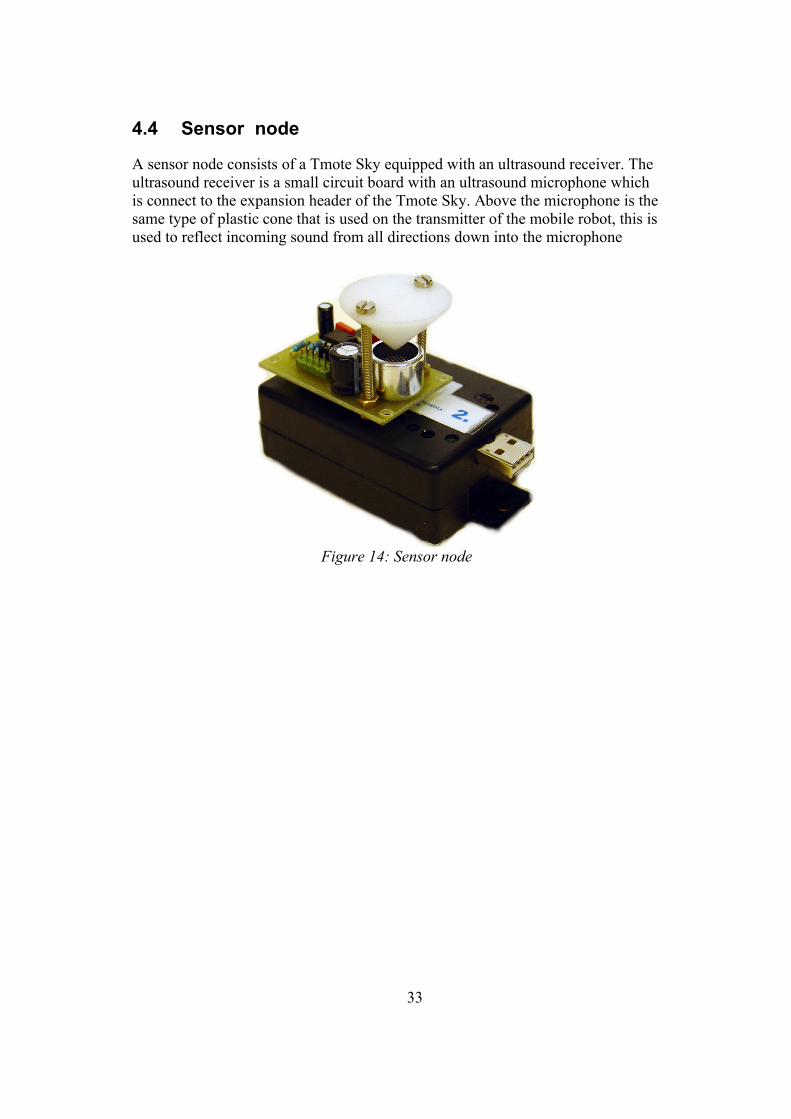
A sensor node consists of a Tmote Sky equipped with an ultrasound receiver. The ultrasound receiver is a small circuit board with an ultrasound microphone which is connect to the expansion header of the Tmote Sky. Above the microphone is the same type of plastic cone that is used on the transmitter of the mobile robot, this is used to reflect incoming sound from all directions down into the microphone

33

Figure 14: Sensor node

5. Software

This chapter describes the software and protocols used on the mobile robot.

5.1 Contiki

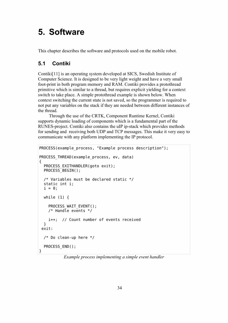
Contiki[11] is an operating system developed at SICS, Swedish Institute of Computer Science. It is designed to be very light weight and have a very small foot-print in both program memory and RAM. Contiki provides a protothread primitive which is similar to a thread, but requires explicit yielding for a context switch to take place. A simple protothread example is shown below. When context switching the current state is not saved, so the programmer is required to not put any variables on the stack if they are needed between different instances of the thread.

Through the use of the CRTK, Component Runtime Kernel, Contiki supports dynamic loading of components which is a fundamental part of the RUNES-project. Contiki also contains the uIP ip-stack which provides methods for sending and receiving both UDP and TCP messages. This make it very easy to communicate with any platform implementing the IP protocol.

PROCESS(example_process, "Example process description");

PROCESS_THREAD(example_process, ev, data){ PROCESS_EXITHANDLER(goto exit); PROCESS_BEGIN();

/* Variables must be declared static */ static int i; i = 0;

while (1) { PROCESS_WAIT_EVENT(); /* Handle events */ i++; // Count number of events received } exit:

/* Do clean-up here */

PROCESS_END();}

Example process implementing a simple event handler

34

5.2 I²C

The different processors on the mobile robot use I²C to communicate. I2C is a simple two wire serial bus developed by Phillips Semiconductors[12]. The protocol is implemented by many other vendors but under different names due to licensing restrictions, for instance the Atmel AVR refer to it as the “two-wire serial interface”[13].

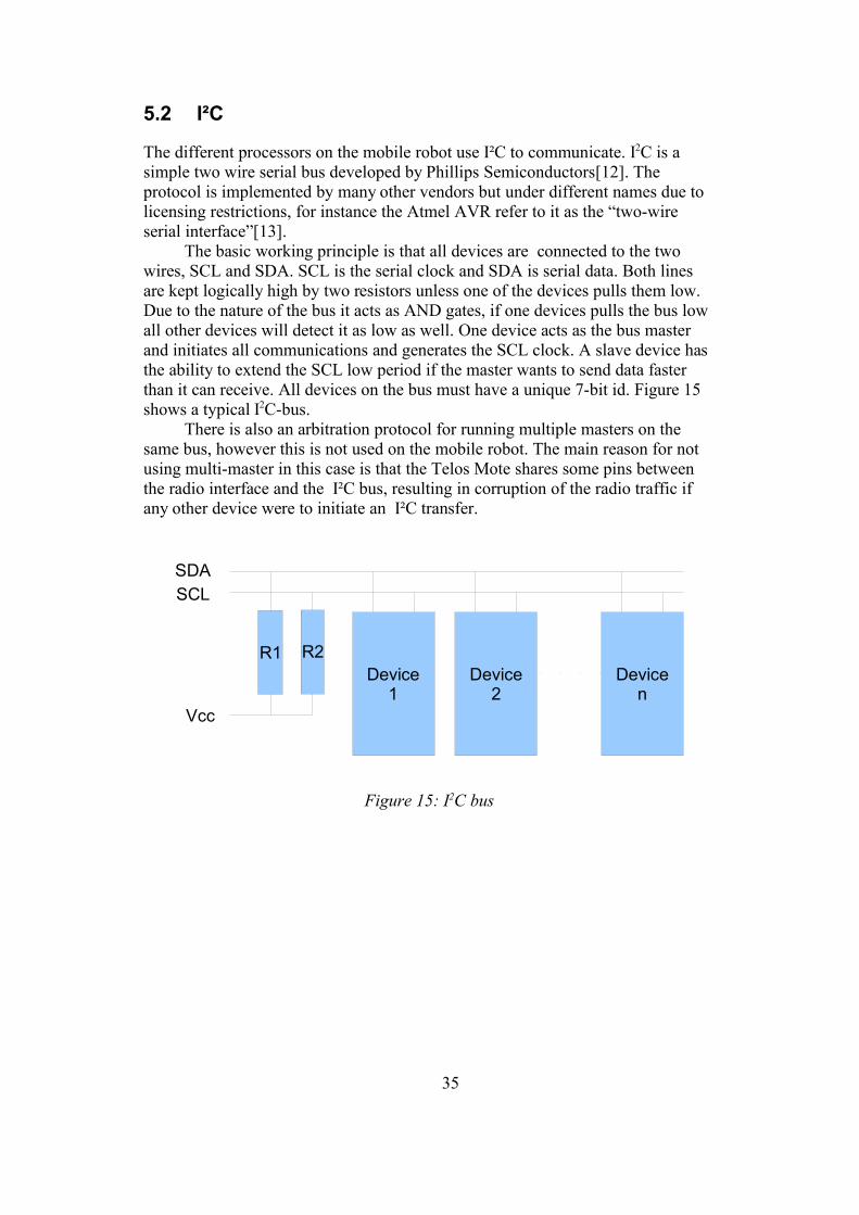
The basic working principle is that all devices are connected to the two wires, SCL and SDA. SCL is the serial clock and SDA is serial data. Both lines are kept logically high by two resistors unless one of the devices pulls them low. Due to the nature of the bus it acts as AND gates, if one devices pulls the bus low all other devices will detect it as low as well. One device acts as the bus master and initiates all communications and generates the SCL clock. A slave device has the ability to extend the SCL low period if the master wants to send data faster than it can receive. All devices on the bus must have a unique 7-bit id. Figure 15 shows a typical I2C-bus.

There is also an arbitration protocol for running multiple masters on the same bus, however this is not used on the mobile robot. The main reason for not using multi-master in this case is that the Telos Mote shares some pins between the radio interface and the I²C bus, resulting in corruption of the radio traffic if any other device were to initiate an I²C transfer.

35

Figure 15: I2C bus

R1 R2

Vcc

SCLSDA

Device2

Device1

Devicen

6. Distance measuring

This chapter discusses the theory and implementation of the range measurements.

6.1 Theory

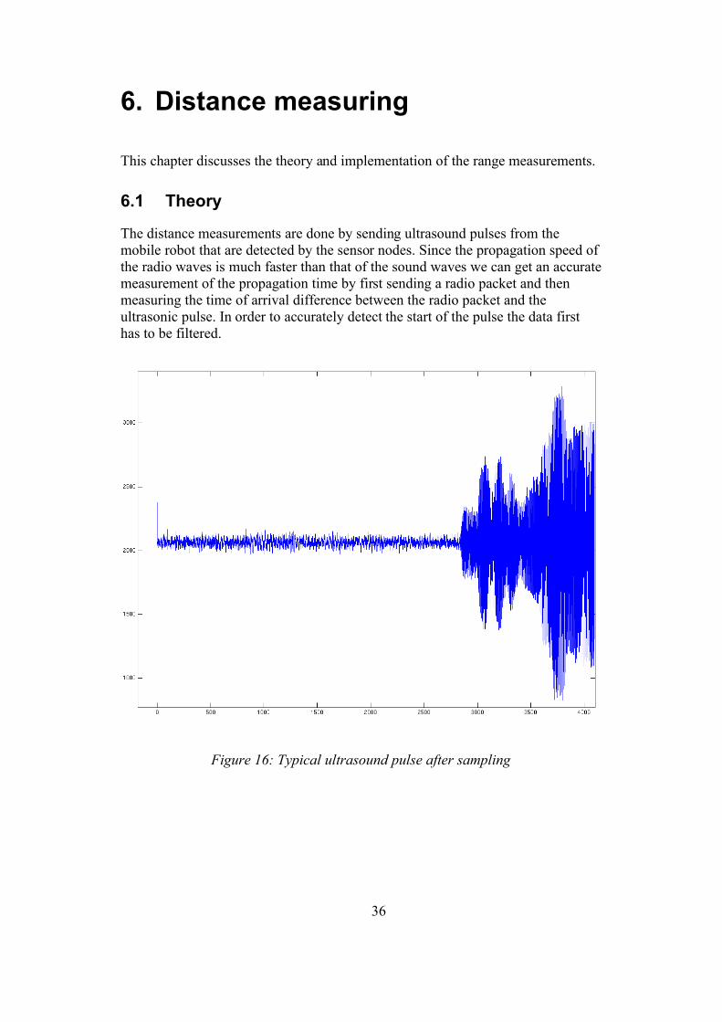
The distance measurements are done by sending ultrasound pulses from the mobile robot that are detected by the sensor nodes. Since the propagation speed of the radio waves is much faster than that of the sound waves we can get an accurate measurement of the propagation time by first sending a radio packet and then measuring the time of arrival difference between the radio packet and the ultrasonic pulse. In order to accurately detect the start of the pulse the data first has to be filtered.

Figure 16: Typical ultrasound pulse after sampling

36

6.2 Implementation

Since the radio packet needs to be sent to all nodes within range UDP packets must be used.

In order to get good accuracy we must have a very deterministic delay between sending our radio packet and the ultrasound pulse. In Contiki the standard procedure for sending a packet is to first request sending and then wait for the process to get an event allowing the transmission. However, due to the timing constraints, in this project an alternative method is used where the actual sending takes place in the calling process context to avoid context switches. This is accomplished by using the function uip_udp_packet_send.

Since there are some delays when sending the radio packages there is a need to wait a specific time before sending the ultrasound pulse, otherwise the pulse will arrive before the radio package. Due to the difficulties in waiting with great accuracy in Contiki this delay is implemented in the Atmel AVR Mega16 that controls the ultrasound transmitter.

The ultrasound is sent by sending a message over the I²C-bus to the Mega16 specifying the duration of the pulse. The Mega16 will, after receiving the message, wait 2 ms and then start outputting the ultrasound pulse under the specified duration.

The detecting node receives the UDP packet and immediately starts sampling the ultrasound receiver and stores the data in an array. The sampled values are filtered by a median-3 filter and compared to a threshold value. The median-3 filer is based on a sliding window of three samples where the filter at every instance chooses the median of the three values within the window. When the filtered absolute value exceeds the threshold the node considers the ultrasound pulse to be detected. The index in the array of sampled value where the pulse is detected is linearly related to the distance the sound traveled.

The slope of the line describing the relation between detection index and distance should only be dependent on the sampling frequency and the speed of sound, our sampling frequency is approximately 73 kHz and the speed of sound is approximately 344 m/s. The offset should be entirely dependent on the delay between sending the UDP packet and the ultrasound pulse.

6.3 Results

In figure 17 we can see that there is a linear relation between the distance and the detection index, as would be expected the standard deviation does not seem to have any correlation with the distance. The detection index is the scale used internally by the system for measuring distances. It should only depend on how deterministic the software running on the transmitter and receiver is. However for large distances there seems to be an increased uncertainty, this also seems to be near the maximum range of the transmitter, which might explain this. Most notable during the experiment was that there is were measurement received for 10

37

meters. At this range 100% packet loss was experienced, radio contact was however regained again when moving the receiver further away. Such dips in the radio reception are hard to predict but are to be expected.

38

Figure 17: Detected index as function of distance

7. Wheel control

This chapter deals with the individual control of the wheels of the mobile robot.

7.1 Hardware

Each wheel of the robot is driven by a single DC-motor. On the wheel-axis there is also a position encoder mounted. The encoder and DC-motor are connected to an Atmel AVR Mega16 processor, the processor is connected to the rest of the system as a slave on an I²C-bus.

The position encoder consists of a dish with 40 alternating black and white fields and two light sensors that measure the reflected light from the dish. The two sensors are mounted so that they are in opposite phase, this results in at least one of the sensors switching from on/off every 1/80th of a revolution.

The position encoder is connected to two analog-to-digital converters on the Mega16. The DC-motor is connected to an analog output.

7.2 Software

Working principleThe software works by continuously reading the values of the analog inputs and comparing them to a reference value to decide whether the sensor currently is reading a black or white field. Every time one of the sensors changes what type of field it is over the position is either incremented of decremented depending on what direction the wheel is moving in. Due to the out of phase nature of the sensors it is possible to determine the direction without any additional information.

With a sampling period of 1 ms the current angular velocity is estimated from the change in position. Due to the discrete nature of the position measurements the velocity estimate is low-pass filtered. The estimated velocity is then compared to the reference velocity and depending on the difference a voltage is calculated and output to the DC-motor.

Existing softwareWhen the master thesis started there was already a P-controller implemented for each wheel. This software however exhibited some problems. When the robot was to run both wheels with the same speed it would drift considerably instead of moving in a straight line. One of the goals of the thesis was to improve this performance.

39

Problems1. When manually turning the wheels the two sides would report different

velocities and one side would sometimes skip some values. The estimated velocity was also much more noisy when doing a step response. The reason for this was that the switching point for the sensors to switch between a black and white field was set to a fixed value, but in reality the sensors had somewhat different offset causing the position estimate to change at the wrong time.

2. When requesting the wheel to move with a certain absolute speed it would depend on whether it was moving in the positive or negative direction.

3. After having fixed problem 1 and 2 the robot would still drift due to differences in friction on the two sides.

4. When doing reference changes the wheels sometimes loose traction, which is a problem when doing dead-reckoning.

Improvements1. To fix the error in position estimate the software stores the maximum and

minimum value recorded from each sensor and uses the average as the switching point between black and white.

2. This effect was due to a rounding error in the fixed-point calculations in the position estimation.

3. The regulator structure was changed to a PI-controller with anti-windup to be able to compensate for load disturbances.

4. A low-pass filter was implemented on the reference velocity.

In addition to the above points the entire controller was re-implemented using fixed-point arithmetics instead of purely integer based math which does not allow for the use of decimals in the numbers. This gives the ability to have somewhat more accurate estimates, but the main advantage is being able to use an integrator with a time constant that is less than one.

40

7.3 Performance

Before the improvements the controller exhibited the following behavior when requested to follow a sequence of reference changes. The tests were done both with the wheels lifted from the ground and with the wheels in contact with the ground so the robot moved in order to test with different load conditions.

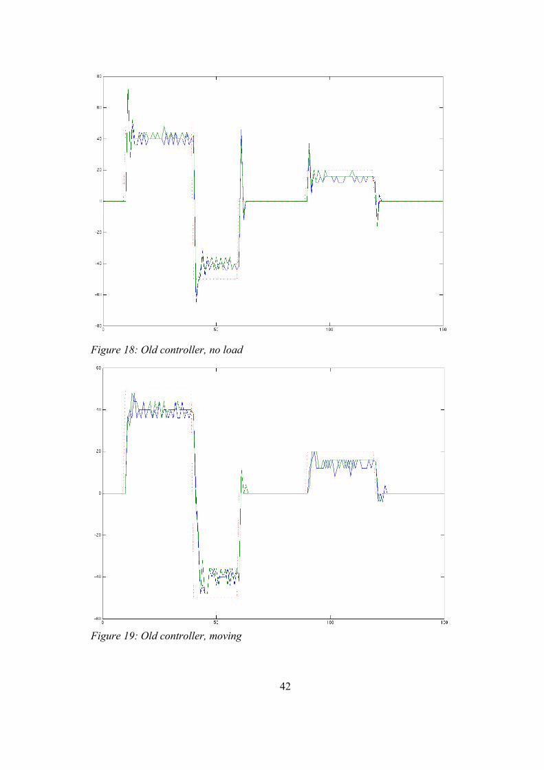
The green line is the speed of the right wheel, the blue that left wheel. The dotted red line is the reference value. The horizontal axis represents time measured in samples, the sampling time being 0.2s. The vertical axis is the velocity, measured in cm/s.

As can be seen in figure 18 and 19 the old controller has problems with overshooting when the load is removed. The two wheels move with slightly different speeds and neither wheel is able to follow the reference value.

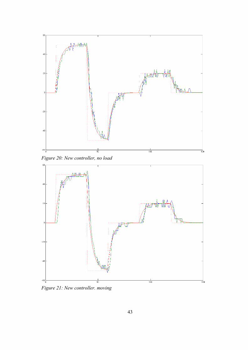
The new regulator introduced filtering of the reference signal, the filtered reference is the solid red line, the unfiltered reference is the dotted red line. As can be seen in figure 20 and 21 the new regulator follows the filtered reference very well and has no stationary errors. There is no noticeable difference between when the robot is moving and when the wheels have been lifted of the floor. There is neither any visible difference between the right and left wheel.

41

42

Figure 18: Old controller, no load

Figure 19: Old controller, moving

43

Figure 20: New controller, no load

Figure 21: New controller. moving

8. Obstacle detection

One of the mobile robots have has equipped with obstacle detection sensors. Currently they consist of a touch sensor bar, which extends over the entire length of the front of the robot, that can detect when the robot has collided with an obstacle. In addition to this the robot is equipped with an IR-distance sensor mounted on an RC-servo. This should be used to sweep the the distance sensor over an arc of 180º in front of the robot creating the ability to make measurements much in the same way that a traditional radar works.

All of the sensors are currently connected to the Atmel AVR that is also responsible for the ultrasound. Due to limitations in the hardware this prevents the servo from being operated at the same time as the ultrasound. Because of this the RC-servo has been disconnected and fixed in the forward looking direction. Since the AVR must act as a slave on the I²C-bus the Telos Mote periodically polls the AVR asking if any obstacle has been detected. This, however, introduce a delay that severely degrades the performance of the obstacle detection.

In the current implementation the mobile robot stops when it detects an obstacle, in the future it is supposed to be integrated with a collision avoidance component developed at the University of Pisa, Italy, which should give it the ability to operate more intelligently. The IR-distance sensor provides an output voltage that depends on the distance to a possible object. This curve is very non-linear, as can be seen in figure 22. Since the rudimentary implementation of the collision detection only needs to know if an object is closer than a certain distance it is only necessary to compare to a fixed value, thus the non-linearity is not a problem.

44

45

Figure 22: Output value from ADC for distance sensor as function of range (m)

9. Robot controller

This chapter describes how the controller for the speed and heading of the mobile robot works.

9.1 Overview

The speed of the robot can be modeled as the average velocity of the two wheels, and the the angular velocity is proportional to the difference in velocity of the two wheels. Using this model it is natural to design two controllers, one for the velocity and one for the angle, the output of the angle controller is then added and subtracted from the two wheels respectively.

9.2 Design

The two wheel controllers have been implemented with reference filtering which gives them a time-constant of 0.5 s independently of the load. The wheels can then be modeled as:

v̇=C vref−v

Using this an LQ-controller is designed for the control of the angle. This controller will depend on the length of the wheel base of the robot, however the only difference will be the constants L1 and L2 which have to be tuned for the individual robot.

udiff =L1ref−−L2ub−ua

9.3 Implementation

The implementation of the controller is just a few lines of C-code which must be called periodically with the same period that was used when designing the controller. Care has to be taken so that the smallest angle difference is always used and that the angle difference never exceeds 180 degrees. This is accomplished by the function angle_diff(angle1, angle2).

46

/* Angle control

u_diff = -L1*X[2]-L2*(u[1]-u[0])+LR*theta_ref = { LR=L1 } =

= L1*(theta-X[2])-L2*(u[1]-u[0])*/

u_diff = L1*angle_diff(theta_ref,X[2]) - L2*(u[1]-u[0]);

if (u_diff > 0) { u_diff = MIN(u_diff, 0.4f);} else { u_diff = MAX(u_diff, -0.4f);}

Source code extract showing controller implementation

47

10. Multiple robots

This chapter discusses how the implementation handles the simultaneous positioning of multiple robots.

10.1 Problem

The ultrasound is a shared resource meaning that there can only be one ultrasonic pulse in the air at any given time. Because the robots are the sender in the positioning scheme this means that if multiple robots are to operate in the same area they must somehow provide a method for guaranteeing that they will not broadcast ultrasonic pulses at the same time. Another issue is that the increased radio traffic might introduce extra delays when doing position estimation.

10.2 Solution

The amount of network traffic is reduced by only sending position information every third iteration of the Kalman predict interval.

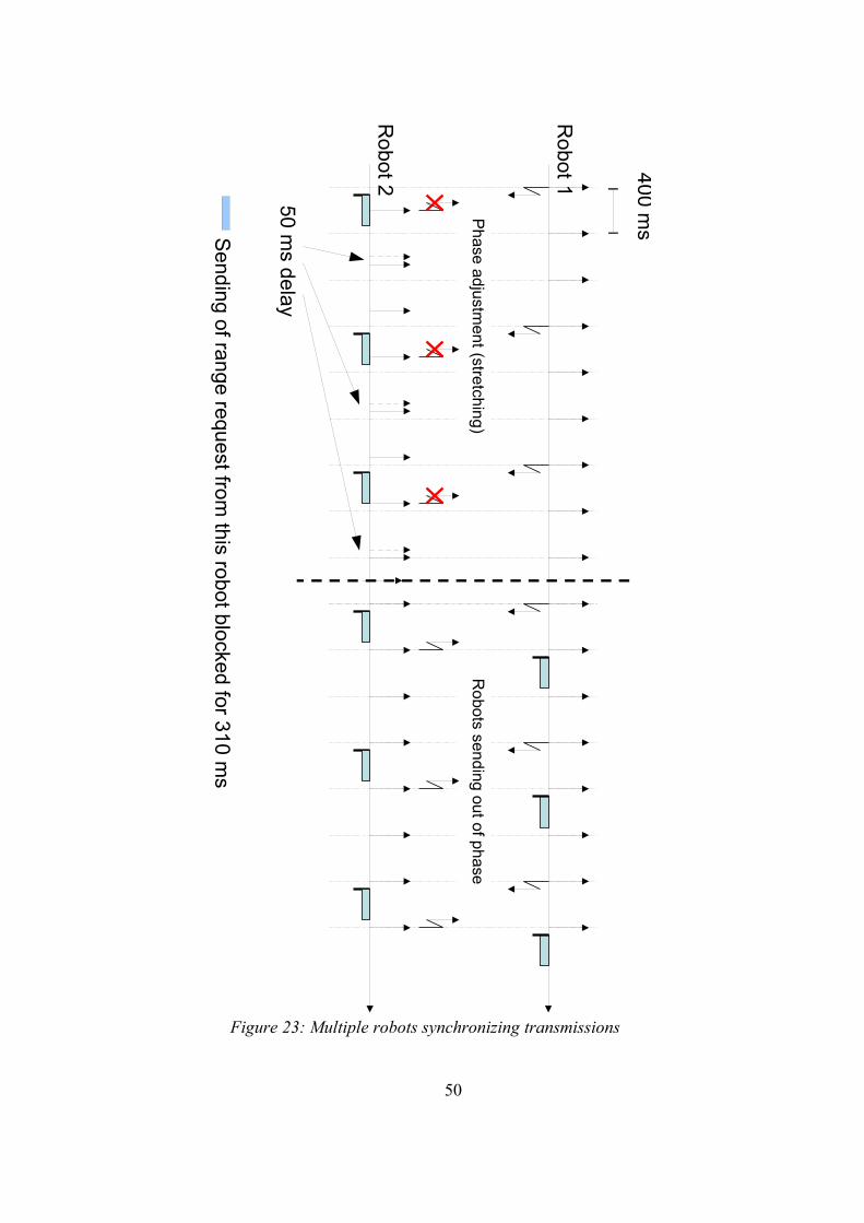
In order to avoid simultaneous ultrasound transmissions all robots listen for the RANGE_REQUEST radio packet that precedes all ultrasound transmissions. Whenever such a packet has been received by a robot that robot will block itself for 310 ms preventing it from making any range requests. After this time the other robot will have finished its request and all the sensor nodes will be ready to make new measurements. This values is based on experimental data on how long time it takes to receive the answers from all the sensor nodes.

If there was another robot that was blocked that wanted to make a measurement while blocked it might end up in a form of starvation where the other robot will always start its measurement slightly before and thus preventing it from ever measuring the position. This problem is solved by temporarily stretching the time period between the Kalman filter iterations every time the robot was blocked when doing a range measurement. The end result of this is that the second robot will eventually have delayed its execution cycle so much that the measurements are done after the blocking time of the other robot.

In the implementation this extra delay is 50 ms, thus the maximum number of missed measurements when running two robots are 7. By using a larger delay it would be possible to escape the blocking situation quicker, however by choosing a smaller value it is possible to be closer in time to the end of the other robots blocking interval. If a too large value is choosen the robot might end up in the next sending interval instead, it also degrades the performance of the Kalman filter as it always calculates using the same fixed time. If the sample time of the Kalman filter is 0.4 s and measurements are done every third iteration, it should be possible to run three robots simultaneously using the values presented above. Since there are only two robots available the algorithm has not been tested with more than two robots.

48

Figure 23 shows a time schedule for two robots doing position estimation. In the beginning Robot2 is unable to make any measurements since it is always blocked by Robot1, however after three attempts its period has drifted far enough to avoid the blocking from Robot1. After that point the two robots are able to make measurements without disturbing each other. The blue rectangles illustrate the time which the robots are blocked by each other. The zigzag shaped arrows illustrate sending of radio packets.

49

50

Figure 23: Multiple robots synchronizing transmissions

Robots sending out of phase

Phase adjustm

ent (stretching)

Robot 1

Robot 2

Sending of range request from this robot blocked for 310 m

s

50 ms delay

400 ms

11. Implementation

This chapter describes how the techniques presented before have been implemented on the mobile robot and nodes.

11.1 Sensor nodes

The main problems with implementing the code in the sensor nodes are to get deterministic delays and to be able respond quickly to the robot without causing unnecessary collisions and network traffic. In order to achieve the deterministic delays the sensor nodes are idle and just waiting until they receive a packet requesting a measurement, then the node immediately starts sampling and saves the results to an array. In order to correctly identify the start of the pulse the values in the array are then filtered. Because of the high sampling rate (~72 kHz) this operation can not be done in real-time, which is the reason that the values are first stored in an array. The filter is a simple Median-3 filter.

After having detected the start of the pulse the node will broadcast the result back using an algorithm described below that avoids collisions with the other nodes without unnecessary network traffic. In order to reduce network traffic all responses are sent as UDP broadcasts, this avoids MAC-level resends and confirmations reducing network traffic. This,however, results in that the packets must somehow be guaranteed to not collide, or they will be lost. Since the robot can not use more than five measurements at the same time there is no reason to send responses from any other nodes than the five closest.

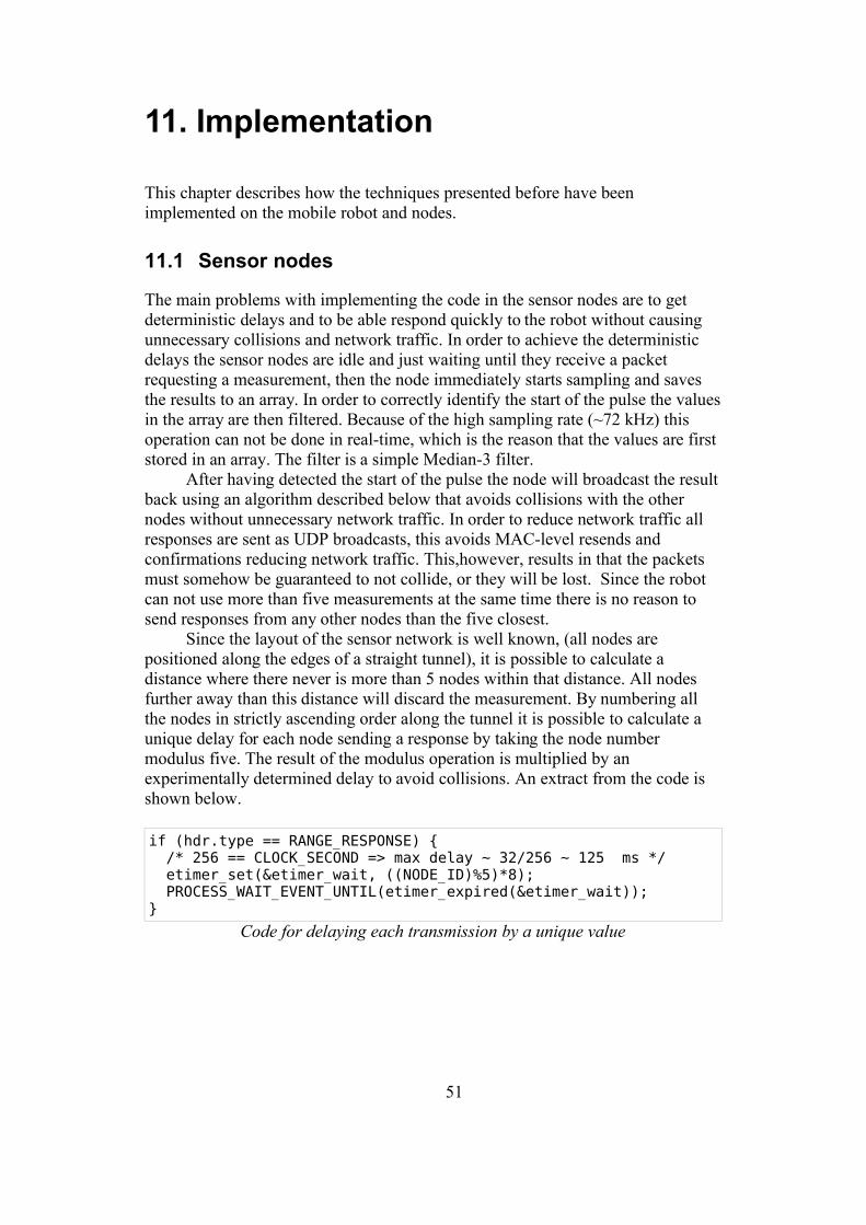
Since the layout of the sensor network is well known, (all nodes are positioned along the edges of a straight tunnel), it is possible to calculate a distance where there never is more than 5 nodes within that distance. All nodes further away than this distance will discard the measurement. By numbering all the nodes in strictly ascending order along the tunnel it is possible to calculate a unique delay for each node sending a response by taking the node number modulus five. The result of the modulus operation is multiplied by an experimentally determined delay to avoid collisions. An extract from the code is shown below.

if (hdr.type == RANGE_RESPONSE) { /* 256 == CLOCK_SECOND => max delay ~ 32/256 ~ 125 ms */ etimer_set(&etimer_wait, ((NODE_ID)%5)*8); PROCESS_WAIT_EVENT_UNTIL(etimer_expired(&etimer_wait));}

Code for delaying each transmission by a unique value

51

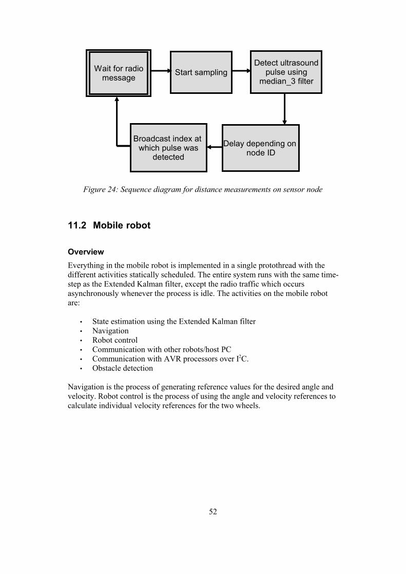
Figure 24: Sequence diagram for distance measurements on sensor node

11.2 Mobile robot

OverviewEverything in the mobile robot is implemented in a single protothread with the different activities statically scheduled. The entire system runs with the same time-step as the Extended Kalman filter, except the radio traffic which occurs asynchronously whenever the process is idle. The activities on the mobile robot are:

• State estimation using the Extended Kalman filter• Navigation• Robot control• Communication with other robots/host PC• Communication with AVR processors over I2C.• Obstacle detection

Navigation is the process of generating reference values for the desired angle and velocity. Robot control is the process of using the angle and velocity references to calculate individual velocity references for the two wheels.

52

Start samplingDetect ultrasound

pulse usingmedian_3 filter

Delay depending on node ID

Broadcast index at which pulse was

detected

Wait for radiomessage

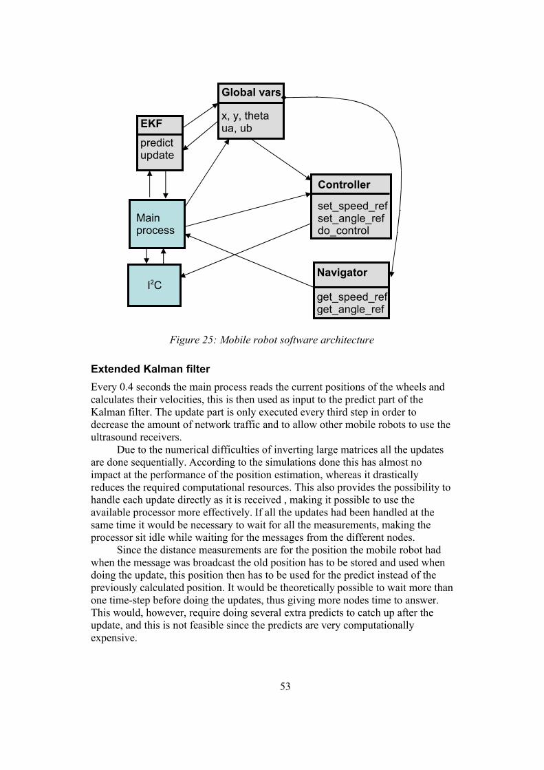
Figure 25: Mobile robot software architecture

Extended Kalman filterEvery 0.4 seconds the main process reads the current positions of the wheels and calculates their velocities, this is then used as input to the predict part of the Kalman filter. The update part is only executed every third step in order to decrease the amount of network traffic and to allow other mobile robots to use the ultrasound receivers.

Due to the numerical difficulties of inverting large matrices all the updates are done sequentially. According to the simulations done this has almost no impact at the performance of the position estimation, whereas it drastically reduces the required computational resources. This also provides the possibility to handle each update directly as it is received , making it possible to use the available processor more effectively. If all the updates had been handled at the same time it would be necessary to wait for all the measurements, making the processor sit idle while waiting for the messages from the different nodes.

Since the distance measurements are for the position the mobile robot had when the message was broadcast the old position has to be stored and used when doing the update, this position then has to be used for the predict instead of the previously calculated position. It would be theoretically possible to wait more than one time-step before doing the updates, thus giving more nodes time to answer. This would, however, require doing several extra predicts to catch up after the update, and this is not feasible since the predicts are very computationally expensive.

53

Main process

I2C

EKF

predictupdate

Global vars

x, y, thetaua, ub

Navigator

Controller

set_speed_refset_angle_refdo_control

get_speed_refget_angle_ref

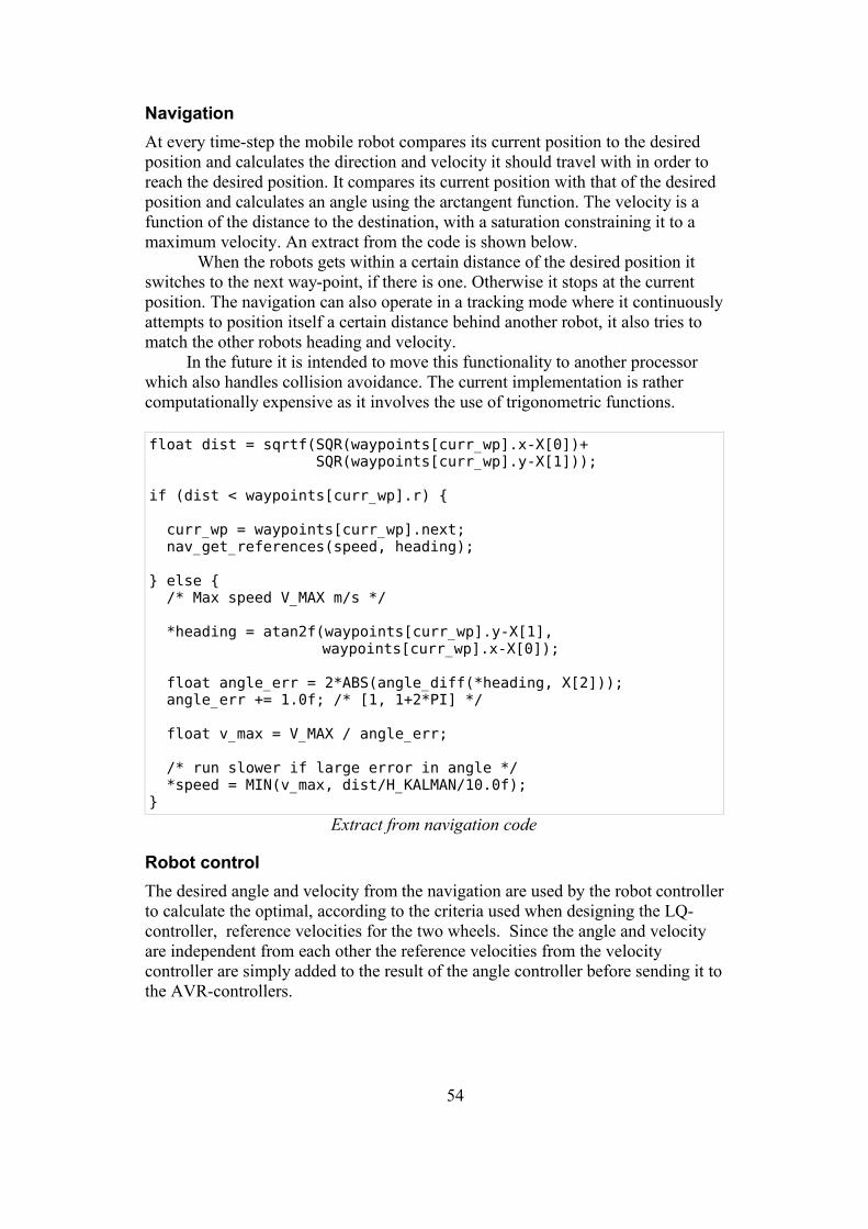
NavigationAt every time-step the mobile robot compares its current position to the desired position and calculates the direction and velocity it should travel with in order to reach the desired position. It compares its current position with that of the desired position and calculates an angle using the arctangent function. The velocity is a function of the distance to the destination, with a saturation constraining it to a maximum velocity. An extract from the code is shown below.

When the robots gets within a certain distance of the desired position it switches to the next way-point, if there is one. Otherwise it stops at the current position. The navigation can also operate in a tracking mode where it continuously attempts to position itself a certain distance behind another robot, it also tries to match the other robots heading and velocity.

In the future it is intended to move this functionality to another processor which also handles collision avoidance. The current implementation is rather computationally expensive as it involves the use of trigonometric functions.

float dist = sqrtf(SQR(waypoints[curr_wp].x-X[0])+ SQR(waypoints[curr_wp].y-X[1]));

if (dist < waypoints[curr_wp].r) {

curr_wp = waypoints[curr_wp].next; nav_get_references(speed, heading);

} else { /* Max speed V_MAX m/s */ *heading = atan2f(waypoints[curr_wp].y-X[1],

waypoints[curr_wp].x-X[0]);

float angle_err = 2*ABS(angle_diff(*heading, X[2])); angle_err += 1.0f; /* [1, 1+2*PI] */

float v_max = V_MAX / angle_err;

/* run slower if large error in angle */ *speed = MIN(v_max, dist/H_KALMAN/10.0f);}

Extract from navigation code

Robot controlThe desired angle and velocity from the navigation are used by the robot controller to calculate the optimal, according to the criteria used when designing the LQ-controller, reference velocities for the two wheels. Since the angle and velocity are independent from each other the reference velocities from the velocity controller are simply added to the result of the angle controller before sending it to the AVR-controllers.

54

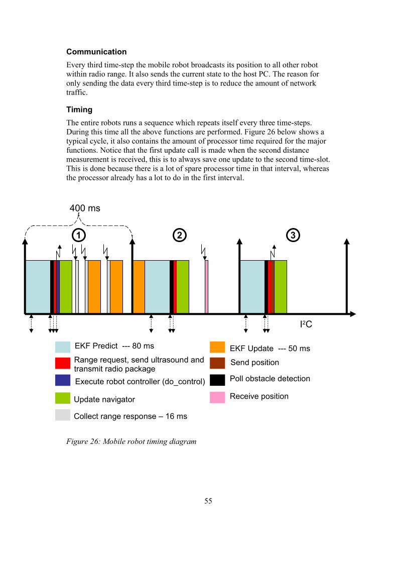
CommunicationEvery third time-step the mobile robot broadcasts its position to all other robot within radio range. It also sends the current state to the host PC. The reason for only sending the data every third time-step is to reduce the amount of network traffic.

TimingThe entire robots runs a sequence which repeats itself every three time-steps. During this time all the above functions are performed. Figure 26 below shows a typical cycle, it also contains the amount of processor time required for the major functions. Notice that the first update call is made when the second distance measurement is received, this is to always save one update to the second time-slot. This is done because there is a lot of spare processor time in that interval, whereas the processor already has a lot to do in the first interval.

Figure 26: Mobile robot timing diagram

55

400 ms

EKF Predict --- 80 ms

Execute robot controller (do_control)

Range request, send ultrasound and transmit radio package

Update navigator

Collect range response – 16 ms

EKF Update --- 50 ms

Send position

1 2 3

I2C

Poll obstacle detection

Receive position

PROCESS_THREAD(rbbot_process, ev, data){ /* Initialisations */

while (1) { PROCESS_WAIT_EVENT(); if (etimer_expired(&etimer_predict)) { predicts++;

/* Use restart, if we are late we don't want to 'catch up' */

etimer_restart(&etimer_predict);

/* calculate estimate of current velocity and store in global u */ get_speeds(u);

switch (predicts % 3) { case 0: case 1: /* Predict current position */ kalman_predict(X,P,u,old_u); /* Do robot control using nav. references*/ mode = ctr_do_control(mode); break; case 2: /* Predict and control will be done after the update */ break; }

switch (predicts % 3) { case 0: /* Send data to host PC */ case 1: /* Send range request */ case 2: /* Calculate kalman_update */ }

/* Save velocity for next time-step */

/* Update navigation */

} if (tcpip_event && uip_newdata()) { /* handle network data, and do asynchronous updates when position messages are received*/ } }}

Mobile robot process, simplified for clarity

56

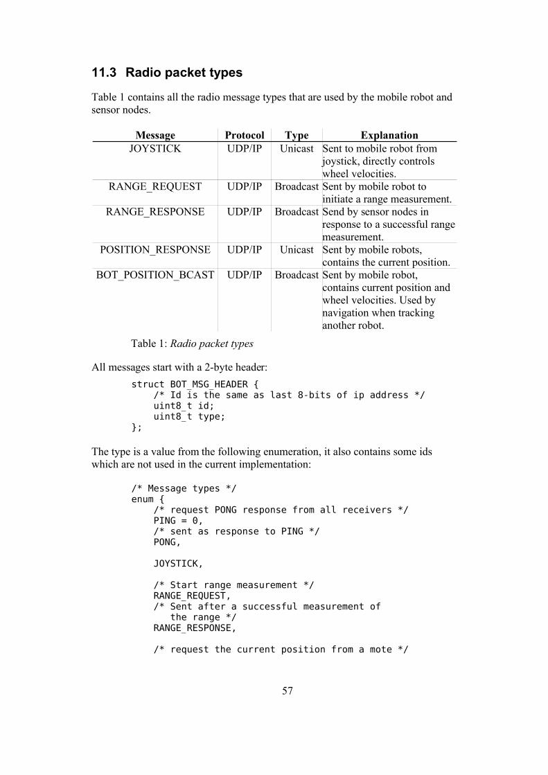
11.3 Radio packet types

Table 1 contains all the radio message types that are used by the mobile robot and sensor nodes.

Message Protocol Type ExplanationJOYSTICK UDP/IP Unicast Sent to mobile robot from

joystick, directly controls wheel velocities.

RANGE_REQUEST UDP/IP Broadcast Sent by mobile robot to initiate a range measurement.

RANGE_RESPONSE UDP/IP Broadcast Send by sensor nodes in response to a successful range measurement.

POSITION_RESPONSE UDP/IP Unicast Sent by mobile robots, contains the current position.

BOT_POSITION_BCAST UDP/IP Broadcast Sent by mobile robot, contains current position and wheel velocities. Used by navigation when tracking another robot.

Table 1: Radio packet types

All messages start with a 2-byte header:struct BOT_MSG_HEADER { /* Id is the same as last 8-bits of ip address */ uint8_t id; uint8_t type;};

The type is a value from the following enumeration, it also contains some ids which are not used in the current implementation:

/* Message types */enum { /* request PONG response from all receivers */ PING = 0, /* sent as response to PING */ PONG,

JOYSTICK,

/* Start range measurement */ RANGE_REQUEST, /* Sent after a successful measurement of the range */ RANGE_RESPONSE,

/* request the current position from a mote */

57

GET_POSITION, /* set the position of a mote */ SET_POSITION,

/* return the current position */ POSITION_RESPONSE,

/* Broadcast our position */ BOT_POSITION_BCAST };

JOYSTICKstruct JOYSTICK_MSG { struct BOT_MSG_HEADER hdr; /* variables should be in the range [-1,1] */ float x; float y;};

RANGE_REQUESTstruct RANGE_REQUEST_MSG { struct BOT_MSG_HEADER hdr;};

RANGE_RESPONSEstruct RANGE_RESPONSE_MSG { struct BOT_MSG_HEADER hdr; /* not the actual range, but the index at

which the pulse is detected */ uint16_t range;

/* Fixed-pint, 9-bit decimal => resolution 1/512 m, which is sufficient since we got a sdev of 0.02 on the range measurements anyhow */

int16_t x; int16_t y;};

58

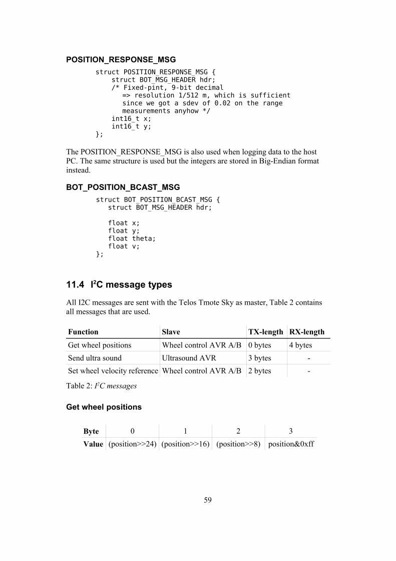
POSITION_RESPONSE_MSGstruct POSITION_RESPONSE_MSG { struct BOT_MSG_HEADER hdr; /* Fixed-pint, 9-bit decimal

=> resolution 1/512 m, which is sufficient since we got a sdev of 0.02 on the range measurements anyhow */

int16_t x; int16_t y; };

The POSITION_RESPONSE_MSG is also used when logging data to the host PC. The same structure is used but the integers are stored in Big-Endian format instead.

BOT_POSITION_BCAST_MSGstruct BOT_POSITION_BCAST_MSG { struct BOT_MSG_HEADER hdr;

float x; float y; float theta; float v;};

11.4 I2C message types

All I2C messages are sent with the Telos Tmote Sky as master, Table 2 contains all messages that are used.

Function Slave TX-length RX-lengthGet wheel positions Wheel control AVR A/B 0 bytes 4 bytesSend ultra sound Ultrasound AVR 3 bytes -Set wheel velocity reference Wheel control AVR A/B 2 bytes -

Table 2: I2C messages

Get wheel positions

Byte 0 1 2 3Value (position>>24) (position>>16) (position>>8) position&0xff

59

Send ultrasoundDuration is in units of 1/40 ms.

Byte 0 1 3Value 0x10 duration>>8 duration&0xff

Set wheel velocity reference

Byte 0 1Value reference>>3 (reference<<5)&0x07

The reference value should be calculated using the following function which takes the velocity (m/s) as input.

/* Given a speed in m/s return the reference value that should send to the motor controller, controller believes 'speed' to be -2*'pos diff'/H, where H = 0.01; encoder_positions / (wheel_diameter*pi)=80*3.183 1 m/s => 255 ticks/s

The reference should thus be: vref * 255 * -2

Zero points is at 1024, with inc. pos. speed <1024 and neg. >1024

Take into consideration the the motors are mounted in opposite directions, and positive vref is always for forward movement. */

uint16_t calc_speed_ref(char motor, float vref){ float tmp = (vref*255.0f*(-2.0f)); if (tmp > 1024.0) tmp = 1024.0; if (tmp < -1024.0) tmp = -1024.0;

/* Add 0.5f to get proper rounding */ if (motor == 'A') return (1024.0f - tmp + 0.5f); else if (motor == 'B')

return (1024.0f + tmp + 0.5f); else return 1024; /* Unknown motor, return zero ref */}

60

12. Experimental results

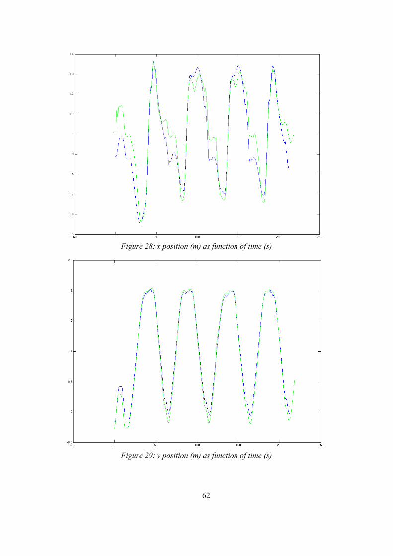
In order to verify the estimation the robot was run in a room with a ceiling mounted camera positioning system. The camera system has an accuracy of approximately 1 cm. In all the following plots the blue curves are the camera estimation and the green curves are the Kalman filter estimation. The two system use different sampling intervals and are not synchronized in time, so the curves have manually been positioned in time to get the best fit. In figure 27 the angle estimate is shown, its accuracy is roughly 15°. As can be seen in figure 28 and 29 the accuracy of the x and y estimates is approximately 10 cm.

To get a better feeling for the performance of the estimation the X and Y position can be simultaneously plotted in a XY-plot, this is done for both experiments that were conducted. This is shown in figure 30 and 31, the scale on the axis is in meters. As can be seen the combined accuracy is worse than for the individual x and y estimates. The position estimation accuracy is roughly 25 cm.

61

Figure 27: angle (radians) as function of time (s)

62

Figure 28: x position (m) as function of time (s)

Figure 29: y position (m) as function of time (s)

63

Figure 30: XY-plot from experiment 1

Figure 31: XY-plot from experiment 2

13. Conclusion

The use of a sensor network for positioning of mobile robots is feasible. The ultrasound based solution used in this thesis is able to provide high enough accuracy for the position estimation, and has been shown to work for two mobile robots at the same time.

The issues of packet loss and malfunction of sensor nodes are handled by implementing dead-reckoning on the robots. The estimates of the dead-reckoning is continuously updated using measurements from the sensor network as they become available.

The main bottle-neck of the current implementation is the performance of the dead-reckoning, especially the estimation of the angle. There are several feasible alternatives for improving this:

– Increasing the accuracy of the robots mechanics, eliminating play in the robot cogwheels. Increasing the precision of the wheel diameters.

– Offloading some calculations of the Extended Kalman filter to another processor. This should make it possible to run dead-reckoning more often, making the model more accurate.

– Adding another method for measuring the angle. There exists simple compasses that can be connected via I2C.

– Including the model for the wheels in the Extended Kalman filter. This should make the model more accurate. After the reference filtering the wheels should be simple include in the model.

64

1 RUNES, Reconfigurable Ubiquitous Network Embedded Sensors, http://www.ist-runes.org/2 Introduction to RUNES, http://www.ist-runes.org/introduction.html3 RUNES participants, http://www.ist-runes.org/participants.html4 A component-based approach to the design of networked control systems, Karl-Erik Årzen, Antonio Bicchi,

Gianluca Dini, Stephen Hailes, Karl H. Johansson, John Lygeros, and Anthony Tzes5 Cricket, http://cricket.csail.mit.edu/6 Triangulation, Wikipedia, http://en.wikipedia.org/wiki/Triangulation7 Trilateration, Wikipedia, http://en.wikipedia.org/wiki/Trilateration8 Multilateration, Wikipedia, http://en.wikipedia.org/wiki/Multilateration9 The Extended Kalman filter, http://en.wikipedia.org/wiki/Kalman_filter10 Moteiv Corporation, http://moteiv.com11 The Contiki Operating System, http://www.sics.se/contiki12 I2C, http://www.nxp.com/products/interface_control/i2c/13 Two-wire serial interface, ATmega8(L) Complete, www.atmel.com