ultrasonic ﬁeld modeling in plates immersed in … · ultrasonic ﬁeld modeling in plates...

International Journal of Solids and Structures 44 (2007) 6013–6029

www.elsevier.com/locate/ijsolstr

Ultrasonic field modeling in plates immersed in fluid q

Sourav Banerjee, Tribikram Kundu *

Department of Civil Engineering and Engineering Mechanics, University of Arizona, Tucson, AZ 85721, USA

Received 4 November 2006; received in revised form 24 January 2007Available online 12 February 2007

Abstract

Distributed Point Source Method (DPSM) is a semi-analytical technique that can be used to calculate the ultrasonicfield (pressure, velocity and displacement fields in a fluid, or stress and displacement fields in a solid) generated by ultra-sonic transducers. So far the technique has been used to model ultrasonic fields in homogeneous and multilayered fluidstructures, and near a fluid–solid interface when a solid half-space is immersed in a fluid. In this paper, the method isextended to model the ultrasonic field generated in a homogeneous isotropic solid plate immersed in a fluid. The objectiveof this study is to model the generation of guided waves in a solid plate when ultrasonic beams from transducers of finitedimension strike the plate at different critical angles. DPSM results for a solid half-space problem are compared with thefinite element predictions to show the superiority of the DPSM technique. The predicted results are also compared with theexperimental visualization of the mode patterns of Lamb waves propagating in a glass plate obtained from stroboscopicphotoelastic method. Experimental and theoretical results show good qualitative agreement. The DPSM technique is thenapplied to study the mode patterns in aluminum plates immersed in water.� 2007 Elsevier Ltd. All rights reserved.

Keywords: Ultrasonic transducers; Fluid–solid interface; Critical angle; Symmetric mode; Anti-symmetric mode; Plate inspection; Guidedwave; Leaky Lamb wave; Numerical modeling

1. Introduction

Modeling of ultrasonic and sonic fields generated by planar transducers of finite dimension is one of thebasic problems in textbooks in this area (Rayleigh, 1965; Morse and Ingard, 1968; Schmerr, 1998; Kundu,2003). A good review of the earlier developments of the ultrasonic field modeling in front of a planar trans-ducer can be found in Harris (1981). A list of more recent developments in this field of research has been givenby Sha et al. (2003). The pressure field in front of a planar transducer in homogeneous isotropic materials hasbeen computed both in the time domain (Stepanishen, 1971; Harris, 1981; Jensen and Svendsen, 1992) and inthe frequency domain (Ingenito and Cook, 1969; Lockwood and Willette, 1973; Scarano et al., 1985; Hah and

0020-7683/$ - see front matter � 2007 Elsevier Ltd. All rights reserved.

doi:10.1016/j.ijsolstr.2007.02.011

q Grant Sponsor: NSF; Grant Nos. CMS-9901221, OISE-0352680 and Air Force Research Laboratory, AFRL/MLLP, through CNDE(Center for Nondestructive Evaluation) of the Iowa State University.

* Corresponding author. Tel.: +1 520 621 6573.E-mail addresses: [email protected] (S. Banerjee), [email protected] (T. Kundu).

mailto:[email protected]

mailto:[email protected]

6014 S. Banerjee, T. Kundu / International Journal of Solids and Structures 44 (2007) 6013–6029

Sung, 1992; Wu et al., 1995; Lerch et al., 1998a,b). In addition to the ultrasonic field modeling in isotropicmaterials progress has been made in the modeling of the ultrasonic radiation field in transversely isotropicand orthotropic media as well (Spies, 1994, 1995). Most of the above-mentioned investigations are basedon Huygen’s principle (Wilcox et al., 1994) where the total field is obtained from the linear sum of pointsources distributed over the transducer. The integral representation of this field is known as Rayleigh–Som-merfield integral. Since numerical integration is a time consuming operation, Wen and Breazeale (1988) pro-posed an alternative approach. They computed the total field by superimposing a number of Gaussian beamsolutions. They have shown that by superimposing only 10 Gaussian solutions the field radiated by a circularpiston transducer can be modeled. Schmerr (2000) followed this approach to compute the ultrasonic field neara curved fluid–solid interface. Later Spies (1999) and Schmerr et al. (2003) extended this technique to a homo-geneous anisotropic solid and water immersed anisotropic solid, respectively. Another technique based onGauss–Hermite beam model for ultrasonic field modeling in anisotropic materials was proposed by Newberryand Thompson (1989).

Although a significant progress has been made in the ultrasonic field modeling in a homogeneous medium,the progress in studying the effect of an interface near an ultrasonic transducer of finite dimension has beenrelatively slow. Recently, Schmerr (2000) and Schmerr et al. (2003) studied the ultrasonic field near a fluid–solid curved interface. Spies (2004) studied the effect of the interface on the ultrasonic wave propagation inan inhomogeneous anisotropic medium with the far field approximation. These investigators followedmulti-Gaussian beam modeling approach. Although this technique has some computational advantage it alsohas a number of limitations similar to those of other paraxial models. For example, it cannot correctly modelthe critical reflection phenomenon; it cannot model a transmitted beam at an interface near grazing incidence.This technique also fails if the interface has different curvatures, or when the radius of curvature of the trans-ducer is small, as observed in acoustic microscopy experiments with its tightly focused lens. A detail descrip-tion of the limitations of the multi-Gaussian paraxial models can be found in Schmerr et al. (2003).

A newly developed technique called Distributed Point Source Method (DPSM), proposed by Placko andKundu (2001, 2003) avoids the above-mentioned limitations and does not require any far field approximation.In this technique one layer of point sources are distributed near the transducer face and two layers are placednear the interface. The advantage of the DPSM technique is that it not only avoids the paraxial approximationit also does not require any ray tracing. All methods developed so far for ultrasonic field radiation modelingnear a fluid–solid interface by point source superposition technique require computation of reflection andtransmission coefficients at the interface (Lerch et al., 1998a,b; Schmerr, 2000; Schmerr et al. 2003; Spies,2004). Ray tracing and reflection/transmission coefficient computation become cumbersome in presence ofmultiple interfaces while such geometries can be relatively easily modeled by the DPSM technique (Banerjeeet al., 2006).

Engineers and scientists are implementing different numerical and semi-analytical techniques such as FiniteElement Method (FEM), Boundary Element Method (BEM) to solve almost all engineering and scientificproblems using high speed computers to reduce computation time and cost. However, the success of the finiteelement method for solving high frequency wave propagation problems has been limited because of the spu-rious reflection of the waves at artificial boundaries and requirements of very small size elements. On the otherhand in BEM, it is required to solve long boundary integral equations that inevitably encounter singularity.To avoid long integral equations and singularities encountered in BEM for complex problems a modifiedBEM known as the Charge Simulation Method (CSM) and a noble semi-analytical technique called MultipleMultipole Program (MMP) (Ballisti, 1983) were proposed. MMP was first proposed for electromagnetic waveproblems by Hafner (1985). Later Imhof (1996, 2004) and Rokhlin (1990) extended the method to acousticsand elastic wave scattering problems in isotropic unbounded media. But with best of authors’ knowledge themethod has never been used for ultrasonic nondestructive problems where elastic waves are generated by finitesize sources. In MMP the contribution from each pole is considered as contribution from each basis functionsobtained from spherical wave function expansion of wave potentials. In MMP the error is minimized and coef-ficients of basis vectors are obtained by enforcing boundary and continuity conditions. Bessel functions andHankel functions are used as basis functions in spherical wave function expansion (Imhof, 1996). If the centerof expansion is located inside the domain of interest, Bessel solutions are used corresponding to standingwaves. In contrast to the propagatory Hankel solutions, the Bessel solutions do not have a singularity and

S. Banerjee, T. Kundu / International Journal of Solids and Structures 44 (2007) 6013–6029 6015

they are evaluated at their origins. Singularity of Hankel functions simulates presence of point sources and theHankel solutions are not used to expand the wave fields in the domain of interest. If the expansion center islocated outside the domain of interest, then the expansion with the Hankel functions can avoid singularities.This method has never been extended to anisotropic materials. Similar to MMP in CSM (Rajamohan andRaamachandran, 1999; Nishimura et al., 2000; Nishimura and Nishimori, 2005; Xu et al., 2002; Okanoet al., 2003) the boundary integral formulation is replaced by assuming suitable polynomial particular integralfunctions. This technique avoids the necessity of discretizing the problem domain as done in BEM. In CSMsuitable number of poles are distributed away from the boundary to satisfy the boundary conditions and toavoid the singularities. The location and distribution of the pole points are quite arbitrary. An ideal selectionof pole points for a particular problem is chosen by trial and error. Only recently an optimization technique(genetic algorithm) is used to determine the arrangement of fictitious charges or poles (Nishimura et al., 2000).Thus, similar to MMP, arrangement of poles or charges in CSM is highly problem dependent and requiresadditional optimization techniques for solving real time ultrasonic field modeling problems. In DPSM tech-nique the point sources are distributed on both sides of the problem boundary and are placed at a constantdistance. Using two layers of point source on two sides of the interface avoids singularity and the need ofreflection and transmission coefficient expressions that are required by other point source superposition basedmethods. This makes DPSM an efficient technique for ultrasonic field modeling.

DPSM technique for ultrasonic field modeling was first developed by Placko and Kundu (2001). They suc-cessfully used this technique to model ultrasonic fields in a homogeneous fluid, and in a nonhomogeneous fluidwith one interface (Lee et al., 2002; Placko et al., 2002) and multiple interfaces (Banerjee et al., 2006). Theinteraction between two transducers, for different transducer arrangements and source strengths, placed ina homogeneous fluid has been studied by Ahmad et al. (2003). The scattered ultrasonic field generated by asolid scatterer of finite dimension placed in a homogeneous fluid has been also modeled by the DPSM tech-nique (Placko et al., 2003). Recently the method has been extended to model phased array transducers(Ahmad et al., 2005). All these works modeled the ultrasonic field in a fluid medium. Only recently, the DPSMtechnique has been extended to model pressure and displacement fields near a fluid–solid interface (Banerjeeet al., 2006). Leaky Rayleigh waves generated at the fluid–solid interface was modeled in this paper. It shouldbe noted here that paraxial based techniques fail to model critical Rayleigh angle reflection phenomenon.

In this paper, the technique is extended to model a homogeneous, isotropic solid plate with fluid–solid inter-faces on both sides of the plate. Our objective is to model the Lamb wave propagation phenomenon in theplate – to see how the energy leaks into the surrounding fluid, how the symmetric and anti-symmetric modesare formed in the plate and how the mode shapes for different Lamb modes vary as the distance of the obser-vation point increases from the transducer position. This calculation requires explicit expressions of stress anddisplacement Green’s functions for fluid and solid media. The ultrasonic fields in a solid plate are calculatedfor critical angles of inclination to generate symmetric and anti-symmetric Lamb modes.

2. Theoretical derivation

A brief review of the Distributed Point Source Method is presented below before specializing it for the plateproblem. For detail description of the technique the readers are referred to other publications (Placko andKundu, 2003; Banerjee et al., 2006; Banerjee and Kundu, 2007) that discuss this technique in greater detail.

2.1. Distributed Point Source Method

If the front face of a transducer is considered as a finite source, then the ultrasonic field due to that finiteplane source can be assumed to be the summation of the ultrasonic fields generated by a number of pointsources distributed near the finite front face. Any interface generates reflected and transmitted ultrasonicfields. Therefore the effect of the interface can be modeled by two layers of sources, one layer generates thereflected field and the second layer generates the transmitted field. By placing two layers of point sourceson two sides of the interface singularities are avoided and no expressions of reflection and transmission coef-ficients are required. These properties distinguish the DPSM technique from other point force superpositiontechniques. Near a fluid–solid interface, with a transducer immersed in the fluid medium, the interface point


sources generate reflected waves in the fluid and transmitted waves in the solid. For solving this problem weneed to calculate the stress and displacement Green’s functions in the solid, and pressure and displacementGreen’s functions in the fluid.

2.1.1. Displacement Green’s functions in the solid

A point source acting in a solid, can be modeled as a concentrated body force,

Fðx; tÞ ¼ Pf ðtÞdðxÞ or F i ¼ P if ðtÞdðxjÞ ð1Þ

where P is the force vector. For harmonic time dependence [f(t) = e�ixt], when the point source is at y then thedisplacement field at x can be expressed in terms of the Green’s functions Gij(x; y),

ui ¼ Uie�ixt ¼ Gijðx; yÞP je

�ixt ð2Þ

The displacement Green’s function for isotropic solids can be written as (Mal and Singh, 1991),

Gijðx; yÞ ¼ 1

4pqx2

eikpr

r k2pRiRj þ ð3RiRj � dijÞ ikp

r � 1r2

� �� þ

eiksr

r k2s ðdij � RiRjÞ � ð3RiRj � dijÞ iks

r � 1r

� �� 24

35 where; Ri ¼

xi � yi

rð3Þ

where, xi are the coordinates at the observation point, yi are the coordinates at the source point, r is the dis-tance between the observation point and the source point, kP is the P-wave number and kS is the S-wave num-ber of the solid. In matrix form,

Gðx; yÞ ¼ ½G1ðx; yÞ G2ðx; yÞ G3ðx; yÞ �T and u ¼ Gðx; yÞP ð4Þ

If the unit excitation force at y acts in the xj direction, then the displacement at x in xi direction is given byGij(x;y).

2.1.2. Stress Green’s functions in the solidFor isotropic homogeneous solids the expression for stresses can be written as

rij ¼ 2leij þ kdijekk ð5Þ

where, k, l are the two Lame constants and dij is the Kronecker Delta. Substituting the expression for displace-ment (Eq. (2)) in the expression for strains, eij ¼ 1

2ðui;j þ uj;iÞ, we get

eij ¼1

2ðGik;j þ Gjk;iÞP k ð6Þ

In the following the time harmonic term e�ixt is implied and is not explicitly written for convenience. Substi-tuting the expression for strains in Eq. (5), the stress Green’s function at x due to a concentrated time har-monic force at y can be obtained.

rijðx; yÞ ¼ ðlðGik;j þ Gjk;iÞdkq þ kdijGkq;kÞP q ð7Þ

Readers are referred to Banerjee et al. (2006) and Banerjee and Kundu (2007) for expressions of the stressGreen’s functions of Eq. (7).

2.1.3. Pressure and displacement Green’s functions in the fluid

Spherical bulk waves in a fluid can be generated by a point source in an infinite fluid medium. If the pointsource is harmonic, then it will generate harmonic spherical waves. The governing differential equation for aharmonic dirac-delta impulsive body force can be written as

r2Gf �1

c2f

€Gf ¼ dðx� yÞe�ixt ð8Þ

where, Gf is the pressure Green’s function in fluid at x due to the point source acting at y.If Gf(r, t) = Gf(r,x)e�ixt then the above equation will have the following solution (Kundu, 2003),


Gfðr;xÞ ¼eikf r

4pr; where kf ¼

xcf

ð9Þ

and the three components of displacement are,

u1 ¼1

4pqx2

1

rikf R1eikf r � eikf r

r2R1

� �ð10Þ

u2 ¼1

4pqx2

1


r2R2

� �ð11Þ

u3 ¼1

4pqx2

1


r2R3

� �ð12Þ

where Ri ¼ xi�yir

2.2. Ultrasonic field modeling in a homogeneous solid plate

Let us consider a plate immersed in an infinite fluid medium. Thus the plate is bounded by two solid–fluidinterfaces. A schematic diagram of the problem geometry considered for our analysis is shown in Fig. 1. Alongthe interfaces two layers of distributed point sources are shown in the diagram.

There are two circular piston transducers immersed in the fluid, symmetrically placed on both sides of theplate specimen. Small circles behind the transducer faces and on both sides of the interfaces show the pointsource locations. Contribution of these sources when superimposed, should produce the total ultrasonic fieldin fluid and solid media. A1 is the source strength vector of the point sources that are placed above the firstsolid–fluid interface and generate the additional ultrasonic field in the fluid below the plate caused due to thepresence of the plate. The interface is called ‘‘Interface 1’’. A�1 is the source strength vector of the sources thatare distributed below the first solid–fluid interface and model the transmitted field in the solid plate. SimilarlyA2 and A�2 are the source strength vectors of the point sources that have been distributed above and below thesecond fluid–solid interface, respectively. This interface is called ‘‘Interface 2’’. Transducer faces have sourcestrength vectors AS and AT. In Fig. 1, three points (C, D and E) have been considered for the illustration pur-pose. The ultrasonic field at point C is the summation of the contributions of the point sources A�1 and A2

distributed below and above the interfaces 1 and 2, respectively. Ultrasonic field at point D is the summation

Fig. 1. Distribution of the point sources at the fluid solid interface of the plate.


of contributions of the point sources A1 and AS distributed above the solid–fluid interface 1 and the transducerface, respectively. Similarly, the Ultrasonic field at point E is the summation of contributions of the pointsources A�2 and AR distributed below the solid–fluid interface 2 and behind the transducer face, respectively.

2.2.1. Matrix formulation to calculate the source strengths

The velocity and pressure in fluids can be expressed in the matrix form when we take a mesh-grid of targetpoints or station points in solid and fluid as shown in Fig. 2. When target points are not necessarily on thetransducer surface, the velocity due to point sources distributed on the transducer face can be written as

F

VT1 ¼MðT1ÞSAS ð13Þ

and due to interface sources,

VT1 ¼MðT1Þ1A1 ð14Þ

where VT1 is the (M · 1) vector of the velocity components at M number of target points distributed inside thefluid or at the fluid–solid interface and AS is the (N · 1) vector containing the strength of the transducersources. The interface has M source points distributed on each side of the interface. Therefore, A1 has(M · 1) elements. M(T1)S and M(T1)1 are two matrices of dimension M · N and M · M, respectively. Elementsof these matrices are functions of the Green’s functions given in Eqs. (10)–(12) and are presented in Banerjeeet al. (2006) and Banerjee and Kundu (2007).

Similarly the pressure at any set of target points in the fluid below the plate due to the transducer sources,can be written as

PRsT1 ¼ QðT1ÞSAS ð15Þ

and due to interface sources, the pressure at the same set of target points in the fluid can be written as

PR1T1 ¼ QðT1Þ1A1 ð16Þ

where, elements of Q(T1)S and Q(T1)1 matrices are functions of the Green’s function given in Eq. (9) and arepresented in Banerjee et al. (2006) and Banerjee and Kundu (2007). T1 and T2 are two different sets of targetpoints in the fluid below and above the Interfaces 1 and 2, respectively. Therefore, at those target points thetotal pressure field is

PRT1 ¼ PRsT1 þ PR1

T1 ¼ QðT1ÞSAS þQðT1Þ1A1 ð17Þ

In the same manner for any set of target points in the fluid above the plate can be written as

ig. 2. A schematic diagram of M source points and N target points inside the solid and the fluid of a fluid–solid structure.


PRT2 ¼ PRsT2 þ PR2�

T2 ¼ QðT2ÞRAR þQðT2Þ2�A�2 ð18Þ

Similarly, at a set of target points, the displacement along the x3 direction in the fluid below and above theplate, can be written as

U3T1 ¼ DF3ðT1ÞSAS þDF3ðT1Þ1A1 ð19ÞU3T2 ¼ DF3ðT2ÞRAR þDF3ðT2Þ2�A

�2 ð20Þ

Elements of DF3(T1)S, DF3(T1)1, DF3(T2)R and DF3(T2)2* matrices are functions of the Green’s functions givenin Eqs. (10)–(12) and are presented in Banerjee et al. (2006) and Banerjee and Kundu (2007).

Each point source that has been considered to calculate the transmitted field in the solid has three differentpoint forces in three different directions as unknowns. The stress along x3 direction at the Interface 1 (the set oftarget points called I1) due to A�1 and A2 source strength vectors, can be written as

s33I1 ¼ S3311�A�1 þ S3312A2 ð21Þ

Similarly, for shear stresses, from Eq. (17), it can be written as

s31I1 ¼ S3111�A�1 þ S3112A2 ð22Þ

s32I1 ¼ S3211�A�1 þ S3212A2 ð23Þ

Elements of matrices S3311� , S3312, S3111� , S3112, S3211� and S3212 are functions of the Green’s functionsgiven in Eq. (7) and are presented in Banerjee et al. (2006) and Banerjee and Kundu (2007). A�1 and A2 arethe source strength vectors of the sources distributed below and above the fluid–solid interfaces, respectively.These vectors have (3M) elements. Equations similar to Eqs. (21)–(23) can be obtained for Interface 2 simplyby substituting subscript 1 by 2 (since the set of target points are now at I2 instead of I1).

Considering the T1 and T2 target points located at I1 and I2 interfaces, respectively, the displacement alongthe x3 direction in the fluid can be written as

U3I1 ¼ DF3ðI1ÞSAS þDF3ðI1Þ1A1 ð24ÞU3I2 ¼ DF3ðI2ÞRAR þDF3ðI2Þ2�A2� ð25Þ

Similarly in the solid at I1 and I2 interfaces the displacements along the x3 direction can be written as

u3I1 ¼ DS3ðI1Þ1�A�1 þDS3ðI1Þ2A2 ð26Þ

u3I2 ¼ DS3ðI2Þ1�A�1 þDS3ðI2Þ2A2 ð27Þ

Elements of matrices DS3ðI1Þ1� , DS3(I1)2, DS3ðI2Þ1� and DS3(I2)2 are functions of the Green’s functions given inEq. (3) and are presented in Banerjee et al. (2006) and Banerjee and Kundu (2007).

2.2.2. Boundary and continuity conditionsAcross the fluid–solid interfaces the displacement normal to the interface should be continuous. Also, at the

interfaces, the normal stress (s33) in the solid and the fluid should be continuous and the shear stresses in thesolid at the interfaces must vanish. If the normal velocities of the two transducer faces are assumed to be VS0

and VR0, then on the surface of the transducer designated as S.

MSSAS þMSIAI ¼ VS0 ð28Þ

transducer designated as R.

MR2�A�2 þMRRAR ¼ VR0 ð29Þ

At the fluid–solid interfaces, from the continuity of the normal stress,

Q1SAS þQ11A1 ¼ �S3311�A�1 � S3312A2 ð30Þ

Q22�A�2 þQ2RAR ¼ �S3321�A

�1 � S3322A2 ð31Þ

Continuity of the normal displacement gives,


DF31SAS þDF311A1 ¼ DS311�A�1 þDS312A2 ð32Þ

DF322�A�2 þDF32RAR ¼ DS321�A

�1 þDS322A2 ð33Þ

and from the vanishing shear stress condition at the fluid–solid interface,

S3111�A�1 þ S3112A2 ¼ 0 ð34Þ

S3211�A�1 þ S3212A2 ¼ 0 ð35Þ

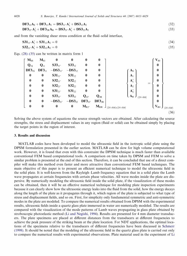
Eqs. (28)–(35) can be written in matrix form 1

MSS MS1 0 0 0 0

Q1S Q11 S3311� S3312 0 0

DF31S DF311 �DS311� �DS312 0 0

0 0 S3111� S3112 0 0

0 0 S3211� S3212 0 0

0 0 S3221� S3222 0 0

0 0 S3121� S3122 0 0

0 0 S3321� S3322 Q22� Q2R

0 0 �DS321� �DS322 DF322� DF32R

0 0 0 0 MR2� MRR

26666666666666666664

37777777777777777775ð2Nþ8MÞxð2Nþ8MÞ

AS

A1

A�1

A2

A�2

AR

8>>>>>>>><>>>>>>>>:

9>>>>>>>>=>>>>>>>>;ð2Nþ8MÞ

¼

VS0

0

0

0

0

0

0

0

0

VR0

8>>>>>>>>>>>>>>>>>>><>>>>>>>>>>>>>>>>>>>:

9>>>>>>>>>>>>>>>>>>>=>>>>>>>>>>>>>>>>>>>;ð2Nþ8MÞ

ð36Þ

Solving the above system of equations the source strength vectors are obtained. After calculating the sourcestrengths, the stress and displacement values in any region (fluid or solid) can be obtained simply by placingthe target points in the region of interest.

3. Results and discussion

MATLAB codes have been developed to model the ultrasonic field in the isotropic solid plate using theDPSM formulation presented in the earlier section. MATLAB can be slow for high volume computationalwork. However, it is found that even with this constraint the DPSM technique is much faster than availableconventional FEM based computational tools. A comparison on time taken by DPSM and FEM to solve asimilar problem is presented at the end of this section. Therefore, it can be concluded that use of a direct com-piler will make this method even faster and more attractive than conventional FEM based techniques. Themain objective of this paper is to present an efficient numerical technique to model the ultrasonic field inthe solid plate. It is well-known from the Rayleigh–Lamb frequency equation that in a solid plate the Lambwave propagates at certain frequencies with certain phase velocities. All wave modes inside the plate are dis-persive. By numerically modeling the ultrasonic field inside the solid plate, if the visualization of these modescan be obtained, then it will be an effective numerical technique for modeling plate inspection experimentsbecause it can clearly show how the ultrasonic energy leaks into the fluid from the solid, how the energy decaysalong the length of the plate as it propagates through it, which region of the plate is subjected to what type ofstress and displacement fields, and so on. First, for simplicity only fundamental symmetric and anti-symmetricmodes in the plate are modeled. To compare the numerical results obtained from DPSM with the experimentalresults, ultrasonic fields inside a quartz glass plate immersed in water are numerically modeled. The results arecompared with the visualization of the mode patterns of Lamb waves propagating in glass plate obtained bystroboscopic photoelastic method (Li and Negishi, 1994). Results are presented for 4 mm diameter transduc-ers. The plate specimens are placed at different distances from the transducers at different frequencies toachieve the peak pressure of the striking beam at the plate location. For NDT applications, the optimal loca-tions of the specimens relative to the transducers of different frequencies have been discussed in Schmerr(1998). It should be noted that the modeling of the ultrasonic field in the quartz glass plate is carried out onlyto compare the numerical results with experimental observations. Plate material used in the experiment of Li


and Negishi (1994) has the same properties as those considered in our model. However, transducer dimensionsand detail problem geometry are slightly different in our modeling from the actual experiment carried out byLi and Negishi (1994). In the experiment the plate was not immersed in water and the transducer was in directcontact with the plate, whereas in computational modeling the plate is immersed in water and the transducersare not in direct contact with the plate. In spite of these differences the results matched reasonably well becauseat low frequencies (below 0.2 MHz) one can see from Fig. 3 that only two modes – one symmetric and oneanti-symmetric mode – can propagate through the plate. Therefore, if the plate is excited symmetrically thenonly S0 symmetric mode and if the plate is excited anti-symmetrically then only A0 anti-symmetric mode isgenerated. No other symmetric or anti-symmetric mode corrupt the propagating S0 and A0 modes. Therefore,the experimental mode shapes presented in Fig. 4 are those for the S0 and A0 modes. Although in the numer-ical modeling the plate is immersed in water and the transducers are not in direct contact with the plate in thiscase also pure A0 and S0 modes are generated by adjusting the angle of inclination of the transducer andmatching the signal frequency with that used in the experiment. When plates are immersed in water the energyleaking into water reduces the strength of the propagating mode but does not significantly affect the modeshape; for this reason the numerical results compared so well with the experimental observation.

P-wave and S-wave speeds of the quartz glass are 5.97 and 3.77 km/s, respectively. Length of the plate is120 mm and its thickness is 10 mm. Dispersion curves for 10 mm thick quartz glass plate immersed in waterare shown in Fig. 3. From Fig. 3 the phase velocities of different modes at various frequencies can be obtained.The phase velocity for the symmetric (S0) mode at 120.4 kHz is 5.824 km/s and that for the anti-symmetric(A0) mode at 170.3 kHz is 2.92 km/s.

The relative positions of the plate and the ultrasonic transducers are shown in Fig. 1. The problem geom-etry considered here has finite size transducers (4 mm diameter). However, the plate length in the in-planedirection and the plate width in the out-of-plane direction are much greater than the transducer diameter.The ultrasonic field is computed along a plane which bisects the transducers and the plate and thus formsa plane of symmetry of the problem geometry. Note that we are solving a 3D problem and plotting the fieldalong the vertical plane of symmetry of the problem geometry. One hundred point sources are distributed neareach transducer face and additional point sources are placed along the plate boundaries as shown in Fig. 1.The question is how many point sources should be used to model the plate boundaries that are extended toinfinity in both in-plane and out-of-plane directions. One plane of point sources at the central plane consists ofseveral lines of point sources as shown in Fig. 1. First the ultrasonic field is computed along the central plane

Fig. 3. Dispersion curves for the 10 mm thick quartz glass plate immersed.

Fig. 4. Visualization of the symmetric (S0) mode at 120.4 kHz and the anti-symmetric mode at 170.3 kHz in a 10 mm thick Glass plate (a)symmetric mode obtained experimentally (after Li and Negishi, 1994). (b) Normal stress difference in the 10 mm thick quartz glass plate at120.4 kHz obtained from DPSM technique. (c) Normal displacement (u3) for symmetric (S0) mode in the 10 mm thick quartz glass plate at120.4 kHz obtained from DPSM technique. (d) Anti-symmetric (A0) mode obtained experimentally (after Li and Negishi, 1994). (b)Normal stress difference for the anti-symmetric (A0) mode in the 10 mm thick quartz glass plate at 170.3 kHz obtained from DPSMtechnique. (c) Normal displacement (u3) for anti-symmetric (A0) mode in the 10 mm thick quartz glass plate at 170.3 kHz obtained fromDPSM technique.


with this one plane of point sources. Then two more planes of point sources are added on two sides of thecentral plane sources and the field is again computed at the central plane. This process of adding two planesof sources on two sides of the central plane is continued until the computed field at the central plane is con-verged. Note that additional source planes on two sides of the central plane only affect the number of pointsources along the plate boundaries. For the two transducers 100 point sources are placed over the transducerface from the very beginning. Interestingly, the results are found to converge with only three planes of sources.However, if one is interested in computing the ultrasonic field at another plane which is not necessarily theplane of symmetry then more planes of sources might be necessary.

On each side of a plate boundary 43 point sources are distributed on the central plane. Sources are placedalong the plate boundaries in the illuminated region and also well beyond the illuminated region. A total of129 sources are then necessary on each side of the plate boundary to model the boundary with 3 planes.


Increasing the number of sources to 215 to construct 5 planes of sources did not significantly change the com-puted ultrasonic field in the central plane. The number of point sources taken for the wave field computation isbased on the convergence criterion of the DPSM technique (Placko and Kundu, 2003). The convergence of theproblem solution has been also tested by increasing the number of point sources in the in-plane direction andat the transducer face. When the spacing between two neighboring point sources is less than the half wave-length then the problem is found to converge. Further increase in the number of point sources did not changethe computed results significantly. For most of the results presented in this paper the distance between twoneighboring point sources has been kept at wavelength/p (approximately 2.8 mm., considering wave velocityin fluid). Thus the results presented in this paper are well converged. Ultrasonic fields in the solid plate areproduced for different striking angles to generate various Lamb wave modes as described below. Results pre-sented below show displacement and stress variations along the length and depth of the plate specimen.

The critical angle of inclination of the transducers are calculated and presented in Table 1. If the transduc-ers are inclined at 14.72� angle the fundamental symmetric mode will be generated in the glass plate. Similarlyif the transducers are inclined at 30.45� angle the fundamental anti-symmetric mode will be generated. Ultra-sonic fields in the glass plate computed by the DPSM technique are presented in Figs. 4(b), (e), (c) and (f). Theexperimental visualization of the same mode patterns are obtained by stroboscopic photoelastic method andpresented in Figs. 4(a) and (d). The difference in normal stresses (r11 � r33) are presented by Li and Negishi(1994) for visualization of the mode patterns. In the DPSM modeling the difference between the two normalstresses in the quartz glass plate are computed and presented in Figs. 4(b) and (e). The vertical displacement(u3) is presented for symmetric and anti-symmetric modes in Figs. 4(c) and (f), respectively. Figs. 4(c) and (f)clearly show the symmetric and anti-symmetric mode patterns. Qualitatitve agreement between the theoreticaland experimental mode patterns should be noted here.

The DPSM technique is then used to model the ultrasonic field in an aluminum plate immersed in waterwhose dispersion curves are shown in Fig. 5. The shear stress variations inside the plate are presented inFig. 6. Properties (density, elastic wave speeds, Lame constants) of the aluminum plate and water are givenin Table 1. The aluminum plate is 50 mm long and immersed in water. Along the abscissa of Fig. 5 the productof frequency and thickness of the plate in MHz-mm is plotted. Along the ordinate the phase velocity in km/s isplotted for different modes. It can be seen from this figure that 1 MHz transducers in a 10 mm thick plate (or5 MHz transducers in a 2 mm thick plate) produce Rayleigh waves for an inclination angle ofsin�1ðcf

crÞ ¼ sin�1ð 1:48

2:916Þ ¼ 30:50�. Shear stress (r31) variations in 10 and 2 mm thick aluminum plates for differ-

ent angles of strike are shown in Fig. 6. Shear stress fields for normal incidence and Rayleigh angle incidenceare shown in Figs. 6(a) and (b), respectively. For normal incidence the shear stress vanishes along both hor-izontal and vertical axes of symmetry, as expected. Propagation of Rayleigh waves on the left side of the pointof strike (brightest regions in the figure) is also evident in Fig. 6(b).

Then a 2 mm thick aluminum plate is considered with 0.5 MHz transducers and point sources are distrib-uted following above-mentioned rule. Fig. 5 shows that the symmetric mode in the 2 mm thick aluminum plate

Table 1Material properties and critical angles for the aluminum and quartz glass plates

Water Quartz glass plate Aluminum plate

P-wave speed 1.48 km/s 5.97 km/s 6.5 km/sS-wave speed 0 3.77 km/s 3.13 km/sDensity 1 g/cc 2.6 g/cc 2.7 g/ccFirst Lame constant (k) — 18.76 GPa 61.17 GPaSecond Lame constant (l) 0 36.95 GPa 26.45 GPaPoission’s ratio (m) — 0.168 0.349Rayleigh wave speed and Rayleigh critical angle 2.916 km/s

— — 30.5�Phase velocity and critical angle considered for symmetric mode — 5.824 km/s 5.333 km/s

14.72� 16.11�Phase velocity and critical angle considered for anti-symmetric mode — 2.92 km/s 2.333 km/s

30.45� 39.43�

Fig. 5. Dispersion curves for an aluminum plate immersed in water.


propagates with a velocity of 5.333 km/s at 0.5 MHz frequency. Therefore, to develop this symmetric mode inthe plate, transducers must be inclined at a critical angle of sin�1ðcf

clÞ ¼ sin�1ð 1:48

5:333Þ ¼ 16:11�. The phase velocity

of the anti-symmetric mode is 2.333 km/s. Therefore, to develop the anti-symmetric mode the transducersmust be inclined at a critical angle of sin�1ðcf

caÞ ¼ sin�1ð 1:48

2:333Þ ¼ 39:43�. Figs. 6(c) and (d) show the shear stress

(r31) developed in the 2 mm thick plate for 39.43� and 16.11� angles of incidence, respectively. Anti-symmetricnature of the plate motion is clearly visible in Fig. 6(c) while in Fig. 6(d) one can see that the shear stress ampli-tude is symmetric about the horizontal central axis.

Fig. 7 shows how the normal displacement and normal stress components at the fluid–solid interface decayalong the length of the plate as the ultrasonic energy travels through the plate away from the point of strike ofthe ultrasonic beam. These results are useful for setting up NDE experiments – such as to decide at which loca-tion the receiver should be placed to receive detectable leaky symmetric and anti-symmetric modes.

A logical question that may arise is whether one can generate visual images like the ones presented in Figs. 4and 6 by the finite element method. The answer is ‘yes but it will be less accurate and will require much morecomputation time’. Most FEM and BEM based techniques do not work efficiently for modeling high fre-quency ultrasonic problems because of spurious reflections at the problem boundaries and the requirementof very large number of elements for discretizing the problem geometry at high frequencies. For these reasonsstandard finite element codes like ABAQUS and ANSYS do not work very well for ultrasonic problems how-ever in recent years specialized finite element codes like PZFLEX (PZFlex, 2001) have been developed to solveultrasonic problems. Since PZFLEX has become a popular FE code for solving ultrasonic problems in spite ofits high cost (about $50,000 licensing fee) a comparison between DPSM results with PZFLEX generatedresults is presented here. A relatively simple problem – ultrasonic field computation near a water–aluminuminterface is solved by these two techniques. DPSM generated results are presented in Fig. 8 for two differentangles of inclination of the transducer. Note that for the incident angle equal to the critical angle(hi = hc = 30.4�) leaky Rayleigh waves are generated (Fig. 8a) and for incident angle (hi = 45.4�) greater thanthe critical angle, the total reflection occurs (Fig. 8b).

Similar results by the finite element code (PZFLEX) are then generated and presented in Fig. 9. Note thatplots in Fig. 9 satisfy two important conditions – (1) guided Rayleigh wave at the fluid–solid interface is gen-erated for critical angle of incidence and (2) total internal reflection is observed for angle of incidence greaterthan the Rayleigh critical angle. These phenomena are also observed in Fig. 8. Thus there is some qualitativeagreement between the DPSM results (Fig. 8) and PZFLEX results (Fig. 9). However, there are some

Fig. 6. Shear stress (r31) variations in 10 mm (top figures) and 2 mm (bottom figures) thick aluminum plate for (a) normal incidence, (b)Rayleigh angle (30.50�) incidence, (c) 39.43� angle of incidence (critical angle for A0 mode) and (d) 16.11� angle of incidence (critical anglefor S0 mode). Transducer frequencies are 1 MHz for the 10 mm thick plate and 0.5 MHz for the 2 mm thick plate.


noticeable differences also between these two sets of results. Note that in Fig. 8a for critical angle of incidencevery little energy penetrates into the solid but in Fig. 9a the level of energy penetrated into the solid is muchhigher. Reflection of the transmitted beam by the artificial top boundary of the solid is also noticeable inFig. 9a. This reflection phenomenon at the problem boundary occurs in spite of using absorbing boundaryconditions. In Fig. 9b the strong energy level near the right boundary is also disturbing.

Clearly, the ultrasonic energy not being absorbed properly by the absorbing boundary causes difficulties inmodeling ultrasonic fields by the finite element method for some problem geometries. However, even moretroubling is to observe in Fig. 9a a strong transmitted wave in the solid for critical Rayleigh angle of incidence.Note that P- and S-critical angles are smaller than the Rayleigh critical angle. Therefore, when the beam isincident at Rayleigh angle P-wave and S-wave beams in the solid should not be present and only negligibleamount of energy should be observed deep inside the solid while most energy should be confined near thefluid–solid interface in the form of the guided Rayleigh wave propagating along the interface and leaking intothe fluid. This is correctly observed in Fig. 8 but not in Fig. 9. Besides these shortcomings another weakness ofFE based codes is that the computational time is much higher than the DPSM based codes. As a comparison itcan be mentioned that the Fig. 8 took 9 min to generate by DPSM whereas Fig. 9 took more than 1 h to gen-erate. Hence, the computation time is an order of magnitude higher for PZFLEX in comparison to that ofDPSM.

This example shows why ultrasonic modeling by the DPSM technique is necessary in spite of manyadvances of FEM based codes in recent years.

Fig. 7. Energy decay along the length of the plate at the fluid–solid interface (a) normal stress (r33), (b) normal displacement (u33).


4. Concluding remarks

Modeling of the complete experimental set up for plate inspection that includes the plate specimen and oneor more ultrasonic transducers of finite dimension immersed in water is not possible analytically. Analyticalsolution is available for Lamb wave propagation in infinite plates with free boundary or leaky Lamb wavepropagation in infinite plates immersed in a fluid. The finite element method (FEM) is the most popular optionavailable today to the scientific community for computing the stress and displacement variations inside theplate generated by a piston ultrasonic transducer of finite diameter. Because of various limitations of FEMin modeling high-frequency ultrasonic experiments its application in ultrasonic experiment modeling has beenlimited. The DPSM modeling presented in this paper opens the door to an efficient alternative technique forultrasonic modeling. Computed results clearly show the symmetric and anti-symmetric modes in the platewhen the transducers are set at appropriate inclination angles. The results also show how the strength ofthe propagating ultrasonic energy decays along the length of the plate because of the energy leakage into

Fig. 8. Ultrasonic fields near a water–aluminum interface generated by the DPSM technique for two different angles of incidence – (a)30.4� (critical angle of incidence) and (b) 45.4�. Leaky Rayleigh waves are clearly visible for the critical angle of incidence (Fig. 7a), (fromBanerjee et al., 2007).

Fig. 9. Ultrasonic fields near the water–aluminum interface (geometry is identical to that of Fig. 7) generated by the PZFLEX FiniteElement code for (a) critical Rayleigh angle of incidence (30.4�) at the water–aluminum interface and (b) for incident angle 45.4� (Resultsgenerated by S. Martin of Air Force Research Laboratory).


the surrounding fluid. Qualitative agreement between the theoretical and experimental results assures the reli-ability of the computation. Comparison of DPSM and FEM predicted results establishes the superiority of theDPSM technique.

Acknowledgements

This research was partially supported from the NSF Grants CMS-9901221, OISE-0352680 and a researchgrant from the Air Force Research Laboratory, AFRL/MLLP, through CNDE (Center for NondestructiveEvaluation) of the Iowa State University. Help of Dr. K. Jata and S. Martin of the Air Force Research Lab-oratory, Dayton, Ohio in generating Fig. 9 is gratefully acknowledged.

References

Ahmad, R., Kundu, T., Placko, D., 2003. Modeling of the ultrasonic field of two transducers immersed in a homogeneous fluid usingdistributed point source method. I2M (Instrumentation, Measurement and Metrology) Journal 3, 87–116.


Ahmad, R., Kundu, T., Placko, D., 2005. Modeling of phased array transducers. Journal of the Acoustical Society of America 117, 1762–1776.

Ballisti, Ch. Hafner, 1983. The multiple multipole method (MMP) in electro and magnetostatic problems. IEEE Transactions onMagnetics 19 (6), 2367.

Banerjee, S., Kundu, T., 2007. Advanced applications of distributed point source method-ultrasonic field modeling in solid media. In:Placko, D., Kundu, T. (Eds.), DPSM for Modeling Engineering Problems, Pub. John Wiley (Chapter 4).

Banerjee, S., Kundu, T., Alnuaimi, N., 2007. DPSM Technique for Ultrasonic Field Modeling near Fluid–Solid Interface, Ultrasonics,under review.

Banerjee, S., Kundu, T., Placko, D., 2006. Ultrasonic field modelling in multilayered fluid structures using DPSM technique. ASMEJournal of Applied Mechanics 73, 598–609.

Ingenito, F., Cook, B.D., 1969. Theoretical investigation of the integrated optical effort produced by sound field radiated from planepiston transducers. Journal of the Acoustical Society of America 45, 572–577.

Jensen, J.A., Svendsen, N.B., 1992. Calculation of pressure fields from arbitrary shaped, apodized, and excited ultrasound transducers.IEEE Transactions on Ultrasonics, Ferroelectric and Frequency Control 39, 262–267.

Hafner, Ch., 1985. MMP calculations of guided waves. IEEE Transactions on Magnetics 21, 2310.Hah, Z.G., Sung, K.M., 1992. Effect of spatial sampling in the calculation of ultrasonic fields generated by piston transducers. Journal of

the Acoustical Society of America 92, 3403–3408.Harris, G.R., 1981. Review of transient field theory for a baffled planar piston. Journal of the Acoustical Society of America 70, 10–20.Imhof, M.G., 1996. Multiple multipole expansions for elastic wave scattering. Journal of the Acoustical Society of America 100, 2969.Imhof, M.G., 2004. Computing the elastic scattering from inclusions using the multiple multipoles method in three dimensions.

Geophysical Journal International 156, 287.Kundu, T. (Ed.), 2003. Ultrasonic Nondestructive Evaluation: Engineering and Biological Material Characterization, CRC Press, Boca

Raton, Florida (Chapter 2).Lee, J.P., Placko, D., Alnuamaini, N., Kundu, T., 2002. Distributed point source method (DPSM) for modeling ultrasonic fields in

homogeneous and non-homogeneous fluid media in presence of an interface. In: Balageas, D.L. (Ed.), First European Workshop onStructural Health Monitoring, Ecole Normale Superieure de Cachan, France, Pub. DEStech, PA, USA, pp. 414–421.

Lerch, T.P., Schmerr, L.W., Sedov, A., 1998a. Ultrasonic transducer radiation through a curved fluid–solid interface. In: Thompson,D.O., Chimenti, D.E. (Eds.), . In: Review of Progress in Quantitative Nondestructive Evaluation, 17A. Plenum Press, NY, pp. 923–930.

Lerch, T.P., Schmerr, L.W., Sedov, A., 1998b. Ultrasonic beam models: an edge element approach. Journal of the Acoustical Society ofAmerica 104, 1256–1265.

Lockwood, J.C., Willette, J.G., 1973. High-speed method for computing the exact solution for the pressure variations in the near field of abaffled piston. Journal of the Acoustical Society of America 53, 735–741.

Li, H.U., Negishi, K., 1994. Visualization of Lamb mode patterns in a glass plate. Ultrasonics 32 (4), 243–256.Mal, A.K., Singh, S.J., 1991. Deformation of Elastic Solids. Prentice Hall, Englewood Cliffs, NJ.Morse, P.M., Ingard, U.K., 1968. Theoretical Acoustics. McGraw-Hill, New York.Newberry, B.P., Thompson, R.B., 1989. A paraxial theory for the propagation of ultrasonic beams in anisotropic solids. Journal of the

Acoustical Society of America 85, 2290–2300.Nishimura, R., Nishimori, K., Ishihara, N., 2000. Determining the arrangement of fictitious charges in charge simulation method using

genetic algorithms. Journal of Electrostatics 49 (2), 95–105.Nishimura, R., Nishimori, K., 2005. Arrangement of fictitious charges and contour points in charge simulation method for electrodes with

3-D asymmetrical structure by immune algorithm. Journal of Electrostatics 63 (6-10), 743–748.Okano, D., Ogata, H., Amano, K., Sugihara, M., 2003. Numerical conformal mappings of bounded multiply connected domains by the

charge simulation method. Journal of Computational and Applied Mathematics 159 (1), 109–117.Placko, D., Kundu, T., 2001. A theoretical study of magnetic and ultrasonic sensors: dependence of magnetic potential and acoustic

pressure on the sensor geometry. Advanced NDE for structural and biological health monitoring, Proceedings of SPIE. In: Kundu, T.(Ed.), SPIE’s 6th Annual International Symposium on NDE for Health Monitoring and Diagnostics, March 4–8, vol. 4335, NewportBeach, CA, pp. 52–62.

Placko, D., Kundu, T., Ahmad, R., 2002. Theoretical computation of acoustic pressure generated by ultrasonic sensors in presence of aninterface. Smart NDE and Health Monitoring of Structural and Biological Systems, SPIE’s 7th Annual International Symposium onNDE and Health Monitoring and Diagnostics, vol. 4702, San Diego, CA, pp. 157–168.

Placko, D., Kundu, T., Ahmad, R., 2003. Ultrasonic field computation in presence of a scatterer of finite dimension. Smart NDE andHealth Monitoring of Structural and Biological Systems, SPIE’s 8th Annual International Symposium on NDE and HealthMonitoring and Diagnostics, vol. 5047, San Diego, CA, pp. 169–179.

Placko, D., Kundu, T., 2003. Modeling of ultrasonic field by distributed point source method. In: Kundu, T. (Ed.), UltrasonicNondestructive Evaluation: Engineering and Biological Material Characterization, Pub. CRC Press, Boca Raton, FL, pp. 144–201(Chapter 2).

PZFlex Software, 2001, Version: 1-j.6, Weilinger Associates.Rajamohan, C., Raamachandran, J., 1999. Bending of anisotropic plates by charge simulation method. Advances in Engineering Software

30 (5), 369–373.Rayleigh, L., 1965. In: Theory of Sound, vol. II. Dover, New York, pp. 162–169.Rokhlin, V., 1990. Rapid solution of integral equations of scattering theory in two dimensions. Journal of Computational Physics 86, 414.


Scarano, G., Denisenko, N., Matteucci, M., Pappalardo, M., 1985. A new approach to the derivation of the impulse response of arectangular piston. Journal of the Acoustical Society of America 78, 1109–1113.

Schmerr, L.W., 1998. Fundamental of Ultrasonic Nondestructive Evaluation-A Modeling Approach. Plenum Press, New York.Schmerr, L.W., 2000. A multigaussian ultrasonic beam model for high performance simulations on a personal computer. Materials

Evaluation, 882–888.Schmerr, L.W., Kim, H.-J., Huang, R., Sedov, A., 2003. Multi-Gaussian ultrasonic beam modeling. In: Proceedings of the World

Congress of Ultrasonics, WCU 2003, Paris, September 7–10, pp. 93–99.Sha, K., Yang, J., Gan, W.-S., 2003. A complex virtual source approach for calculating the diffraction beam field generated by a

rectangular planar source. IEEE Transactions on Ultrasonics, Ferroelectrics, and Frequency Control 50, 890–895.Spies, M., 1994. Transducer-modeling in general transversely isotropic media via point-source-synthesis theory. Journal of Nondestructive

Evaluation 13, 85–99.Spies, M., 1995. Elastic wave propagation in transversely isotropic media II: the generalized Rayleigh-function and an integral

representation for the transducer field theory. Journal of the Acoustical Society of America 97, 1–13.Spies, M., 1999. Transducer field modeling in anisotropic media by superposition of Gaussian base functions. Journal of the Acoustical

Society of America 105, 633–638.Spies, M., 2004. Analytical methods for modeling of ultrasonic nondestructive testing of anisotropic media. Ultrasonics 42, 213–219.Stepanishen, P.R., 1971. Transient radiation from piston in an infinite planar baffle. Journal of the Acoustical Society of America 49,

1627–1638.Wen, J.J., Breazeale, M.A., 1988. A diffraction beam field expressed as the superposition of Gaussian beams. Journal of the Acoustical

Society of America 83, 1752–1756.Wilcox, P., Monkhoue, R., Lowe, M., Cawley, P., 1994. The use of Hygen’s principle to model the acoustic field from interdigital Lamb

wave transducers. Reviews of Progress in QNDE 17, 915–923.Wu, P., Kazys, R., Stepinski, T., 1995. Analysis of the numerically implemented angular spectrum approach based on the evaluation of

two-dimensional acoustic fields. Part I. Errors due to the discrete fourier transform and discretization. Journal of the AcousticalSociety of America 99, 1139–1148.

Xu, W., Zhao, Y., Du, Y., Kagawa, Y., Wakatsuki, N., Park, K.C., 2002. Electrical impedance evaluation in a conductive-dielectric halfspace by the charge simulation method. Engineering Analysis with Boundary Elements 26 (7), 583–590.

ultrasonic ﬁeld modeling in plates immersed in … · ultrasonic ﬁeld modeling in plates...

Documents