ultiscale odel imul vol. 16, no. 1, pp. 1{27 time markov

Copyright © by SIAM. Unauthorized reproduction of this article is prohibited.

MULTISCALE MODEL. SIMUL. c© 2018 Society for Industrial and Applied MathematicsVol. 16, No. 1, pp. 1–27

STATIONARY AVERAGING FOR MULTISCALE CONTINUOUSTIME MARKOV CHAINS USING PARALLEL REPLICA DYNAMICS∗

TING WANG† , PETR PLECHAC† , AND DAVID ARISTOFF‡

Abstract. We propose two algorithms for simulating continuous time Markov chains in thepresence of metastability. We show that the algorithms correctly estimate, under the ergodicityassumption, stationary averages of the process. Both algorithms, based on the idea of the parallelreplica method, use parallel computing in order to explore metastable sets more efficiently. Thealgorithms require no assumptions on the Markov chains beyond ergodicity and the presence of iden-tifiable metastability. In particular, there is no assumption on reversibility. For simpler illustrationof the algorithms, we assume that a synchronous architecture is used throughout the paper. Wepresent error analyses, as well as numerical simulations on multiscale stochastic reaction networkmodels in order to demonstrate consistency of the method and its efficiency.

Key words. Markov chains, Monte Carlo, reversibility, stationary distribution, metastability,parallel replica, stochastic reaction networks, multiscale dynamics, coarse graining

AMS subject classifications. 60J22, 65C05, 65Z05, 82B31, 92E20

DOI. 10.1137/16M1108716

1. Introduction. We focus on computing stationary averages of continuous timeMarkov chains in a synchronous architecture. More precisely, if π is the stationarydistribution of a continuous time Markov chain (CTMC) and f is a function onthe state space, we aim at estimating the average π(f) ≡ Eπ[f ] by taking a timeaverage on a long trajectory of the CTMC. There are many methods for computingstationary averages of stochastic processes. However, the vast majority of them rely onreversibility of the process, e.g., as in Markov chain Monte Carlo [19]. Computationalcost of the ergodic (trajectory) averaging becomes prohibitive when the convergence tothe stationary distribution is slow due to metastability of the dynamics, for example,in the presence of rare events or large time scale disparities (multiscale dynamics)[20]. A possible remedy for these issues is to use parallel computing in order toaccelerate sampling of the state space. For instance, the parallel tempering method(also known as the replica exchange) [12, 10, 9, 17] has been successfully applied tomany problems by simulating multiple replicas of the original systems, each replicaat a different temperature. However, the method requires the time reversibility of theunderlying processes, which is typically not true for processes that model chemicalreaction networks or systems with nonequilibrium steady states. In fact, there arenot many methods that parallelize Monte Carlo simulation for irreversible processeswith metastability, in particular if long-time sampling, such as ergodic averaging,is required. We present a parallel computing approach for CTMCs without timereversibility. One advantage of the proposed algorithms is that they may be used,in principle, on arbitrary CTMCs. The same idea applies to the continuous state

∗Received by the editors December 20, 2016; accepted for publication (in revised form) October6, 2017; published electronically January 2, 2018.

http://www.siam.org/journals/mms/16-1/M110871.htmlFunding: The first author was supported by the U.S. Department of Energy, Office of Science,

Office of Advanced Scientific Computing Research, Applied Mathematics program under contractDE-SC0010549. The second author was partially supported by DARPA project W911NF-15-2-0122.The third author was supported by the National Science Foundation via award NSF-DMS-1522398.†University of Delaware, Newark, DE 19716 ([email protected], [email protected]).‡Colorado State University, Fort Collins, CO 80523 ([email protected]).

1

Dow

nloa

ded

02/0

6/18

to 1

29.8

2.28

.144

. Red

istr

ibut

ion

subj

ect t

o SI

AM

lice

nse

or c

opyr

ight

; see

http

://w

ww

.sia

m.o

rg/jo

urna

ls/o

jsa.

php

http://www.siam.org/journals/mms/16-1/M110871.html

mailto:[email protected]




2 TING WANG, PETR PLECHAC, AND DAVID ARISTOFF

space Markov processes. However, gains in efficiency can occur only if the process ismetastable.

In this contribution we consider only models described by CTMCs. As a mo-tivating example we study a multiscale chemical reaction network model in whichmolecules of different types react with different rates depending on their concentra-tions and reaction rate constants. In this model metastability emerges due to theinfrequent occurrence of reactions with small rates which makes the relaxation to thesteady state dynamics extremely slow. In the transient regime the finite time distri-bution can be approximated using the stochastic averaging technique [24, 14], or thetau-leap method [18]. However, the former does not apply for stationary distribu-tion estimation and that the error they introduce on the stationary state is generallydifficult to evaluate; the latter can still be computationally expensive for long-timesimulations. It is thus desirable to have an efficient algorithm for computing thestationary averages. Thus the proposed algorithm will provide a new multiscale sim-ulation method (in particular for stationary averaging estimation) for the stochasticreaction networks community.

The presented approach builds on the parallel replica (ParRep) dynamics intro-duced in the context of molecular simulations in [22]. The ParRep method used in thecontext of stochastic differential equations, e.g., Langevin dynamics, was rigorouslyanalyzed in [15, 16]. The algorithm we present and analyze builds on the recent workof [1, 2] where the ParRep process was studied for discrete-time Markov chains. Inour algorithms, each time the simulation reaches a local equilibrium in a metastableset W , R independent replicas of the CTMC are launched inside the set allowing forparallel simulations of the dynamics at this stage. The main contribution of this workis a procedure for using the replicas in order to efficiently and consistently estimatethe exit time and exit state from W , along with the contribution to the stationarytime average of f from the time spent in W . We emphasize that we are able to handlearbitrary functions (or observables) on the state space, not only those that are piece-wise constant, i.e., assuming a single value in each W . In the best case, if there are Rreplicas, then the simulation leaves a metastable set about R times faster comparedto a direct serial simulation. The consistency of our algorithms relies on certain prop-erties of the quasi-stationary distribution (QSD) which are essentially local equilibriaassociated with the metastable sets.

We propose two algorithms for computing π(f), called CTMC ParRep and em-bedded ParRep. The former uses parallel simulation of the CTMC, while the latteremploys parallel simulation of its embedded chain, which is a discrete time Markovchain (DTMC). CTMC ParRep (resp., embedded ParRep) relies on the fact that,starting at the QSD in a metastable set, the first time to leave the set is an ex-ponential (resp., geometric) random variable and independent of the exit state; seeTheorem 2.5 below. The algorithms require some methods for identifying metastablesets, though this need not be done a priori—it is sufficient to identify when the CTMCis currently in a metastable set, and when it exits such set. While both algorithms canbe useful for efficient simulation of π(f) in the presence of metastability, we expectthe embedded ParRep can be significantly more efficient, especially when combinedwith a certain type of QSD sampling, called Fleming–Viot [3, 4]. Though we focushere on the computation of π(f), we note that one of our algorithms, CTMC Par-Rep, can be used to compute the dynamics of the CTMC on a coarse space in whicheach metastable set is considered a single (meta-)state. See the discussion belowAlgorithm 1.

The advantages of the proposed algorithms include: (a) no requirement of time

Dow

nloa

ded

02/0

6/18

to 1

29.8

2.28

.144

. Red

istr

ibut

ion

subj

ect t

o SI

AM

lice

nse

or c

opyr

ight

; see

http

://w

ww

.sia

m.o

rg/jo

urna

ls/o

jsa.

php


PARALLEL REPLICA METHODS FOR CTMC 3

reversibility for the underlying dynamics; (b) they are suitable for long-time sam-pling; (c) they may be used, in principle, on arbitrary CTMCs in the presence ofmetastability.

In section 2, we briefly review CTMCs before defining QSDs and detailing relevantproperties thereof. In section 3, we present CTMC ParRep, and study how the errorin the algorithm depends on the quality of QSD sampling. In section 4, we presentembedded ParRep and provide an analogous error analysis. We detail some numericalexperiments on multiscale chemical reaction network model in section 5 in order todemonstrate the consistency and accuracy of the algorithms.

2. Background and problem formulation.

2.1. Continuous time Markov chains. Throughout this paper, X(t) is anirreducible and positive recurrent CTMC with values in a countable set E and πdenotes the stationary distribution of X(t). We are interested in computing stationaryaverages π(f) for a bounded function f : E → R by using the ergodic theorem

(1) limt→∞

1t

∫ t

0f(X(s))ds = π(f),

which holds almost surely for any initial distribution of X(t). The jump times τn andholding times ∆τn for X(t) are defined recursively by

τ0 = 0, τn = inf{t > τn−1 : X(t) 6= X(τn−1)},

and∆τn−1 = τn − τn−1

for n ≥ 1. We assume that X(t) is nonexplosive, that is, limn τn = ∞ almost surelyfor every initial distribution of X(t). This precludes the possibility of infinitely manyjumps in finite time. We denote Xn = X(τn) the embedded chain of X(t). It is easyto see that Xn is a DTMC.

Recall that X(t) is completely determined by its infinitesimal generator matrixQ = {q(x, y)}x,y∈E . Recall that by convention q(x,x) is chosen such that

∑y q(x, y) =

0 and we write q(x) := −q(x, x). Note that irreducibility implies q(x) > 0 for all x ∈E. It is easy to check thatXn has the transition probability matrix P = {p(x, y)}x,y∈Esatisfying

p(x, y) =

{q(x,y)q(x) , x 6= y,

0, x = y.

We state the following well-known fact for the later reference.

Lemma 2.1. For a CTMC X(t) with the corresponding embedded Markov chainXn, the holding time between successive jumps ∆τ0,∆τ1, . . . ,∆τi, . . . are independentconditioned on the embedded chain Xn. Moreover, ∆τi|{Xn} is exponentially dis-tributed with the rate q(Xi) and hence E [∆τi|{Xn}] = q(Xi)−1.

For details on the above facts, see, for instance, [5].

2.2. The quasi-stationary distribution and metastability. Below, we writeP, E for various probabilities and expectations, the precise meaning of which will beclear from context. We use a superscript Pξ, Eξ to indicate that the initial distributionis ξ. When the initial distribution is δx, we write Px, Ex. The symbol ∼ will indicate

Dow

nloa

ded

02/0

6/18

to 1

29.8

2.28

.144

. Red

istr

ibut

ion

subj

ect t

o SI

AM

lice

nse

or c

opyr

ight

; see

http

://w

ww

.sia

m.o

rg/jo

urna

ls/o

jsa.

php



equality in probability law. Re(·) and | · | denote the real part and modulus of acomplex number.

Our ParRep algorithms rely on certain properties of quasi-stationary distribu-tions, which we now briefly review. Let W ⊂ E be fixed and consider the first exittime of X(t) from W , that is,

T = inf{t > 0;X(t) /∈W}.

We consider also the first exit time of Xn from W ,

N = inf{n > 0;Xn /∈W}.

A QSD of X(t) in W (or Xn in W ) is defined as follows.

Definition 2.2. A probability distribution ν with support in W is a QSD forX(t) in W if for each y ∈W and t > 0,

(2) ν(y) = Pν(X(t) = y |T > t).

Similarly, a probability distribution µ with support in W is a QSD for Xn in W if foreach y ∈W and n > 0,

(3) µ(y) = Pµ(Xn = y |N > n).

Throughout, we write ν for a QSD of the CTMC X(t) and µ for a QSD of theembedded chain Xn. The associated set W will be implicit since no ambiguities shouldarise. We will write

(4) νt(A) = Px(X(t) ∈ A |T > t)

for the distribution of X(t) conditioned on T > t, and

(5) µn(A) = Px(Xn ∈ A |N > n)

for the distribution of Xn conditioned on N > n. Notice we do not make explicit thedependence on the starting point x.

We summarize existence, uniqueness, and convergence properties of the QSD inTheorem 2.3 below (see [6, 21]). In Theorem 2.3 below, for simpler presentation, weassume W is finite. That allows us to characterize convergence to the QSD of X(t)and Xn in terms of spectral properties of their generator and transition matrices. Weemphasize, however, there exists more general results to guarantee the convergenceto the QSD and hence the finiteness of W is not necessary for consistency of thealgorithms proposed in this paper.

Recall that Q is the infinitesimal generator matrix of X(t) and P is the transitionprobability matrix of the DTMC Xn. We denote QW = {qxy}x,y∈W and PW ={pxy}x,y∈W the restrictions of P and Q to W .

Theorem 2.3. Let W be finite and nonabsorbing for X(t), and assume PW isirreducible.

(a) The eigenvalues λ1, λ2, . . . of QW can be ordered so that

0 > λ1 > Re(λ2) ≥ . . . ,

where λ1 has the left eigenvector ν which is a probability distribution on W .Moreover, ν is the unique QSD of X(t) in W , and for all x, y ∈W ,

(6) |νt(y)− ν(y)| = |Px(X(t) = y|T > t)− ν(y)| ≤ C(x)e−(λ1−β)t,

Dow

nloa

ded

02/0

6/18

to 1

29.8

2.28

.144

. Red

istr

ibut

ion

subj

ect t

o SI

AM

lice

nse

or c

opyr

ight

; see

http

://w

ww

.sia

m.o

rg/jo

urna

ls/o

jsa.

php



with C(x) a constant depending on x, and β any real number satisfyingRe(λ2) < β < λ1.

(b) Suppose PW is also aperiodic. Then the eigenvalues σ1, σ2, . . . of PW can beordered so that

1 > σ1 > |σ2| ≥ . . . ,

where σ1 has the left eigenvector µ which is a probability distribution on W .Moreover, µ is the unique QSD of Xn in W and for all x, y ∈W ,

(7) |µn(y)− µ(y)| = |Px(Xn = y|N > n)− µ(y)| ≤ D(x)(γ

σ1

)n,

with D(x) a constant depending on x, and γ any real number satisfying |σ2| <γ < σ1.

Proof. We first justify the expression for the eigenvalues. Observe that for x 6=y ∈W , we have q(x, y) > 0 if and only if p(x, y) > 0. It follows that QW is irreducibleif and only if PW is irreducible; see Definition 2.1 in [21]. Now let I be the all onescolumn vector, I(x) = 1 for x ∈ W . Recall that q(x, y) ≥ 0 for every x 6= y ∈ Eand

∑y q(x, y) = 0 for every x ∈ E. This implies that QW I ≤ 0 componentwise.

Since W is nonabsorbing, for some x ∈ W and y /∈ W we have q(x, y) > 0, and itfollows that

∑z∈W q(x, z) < 0. This shows that at least one component of QW I is

strictly negative. The expression for the eigenvalues, and the fact that ν is signed(hence a probability distribution, after normalization) now follows from Theorem 2.6of Seneta [21].

To see ν is the QSD for X(t) in W , we define the stopped process XT (t) = X(t∧T )such that X(t) is absorbed outside W . For any x, z ∈ E, let Ix be the columnvector Ix(z) = 1 if x = z and Ix(z) = 0 otherwise. Finiteness of W ensures thatPx(XT (t) = y) = I ′xe

QW tIy. Thus, for each y ∈W ,

Pν(X(t) = y, T > t) = Pν(XT (t) = y) = νeQW tIy = eλ1tν(y)

andPν(T > t) = Pν(XT (t) ∈W ) = eλ1t,

which leads to ν(y) = Pν(X(t) = y|T > t).Now we turn to the convergence to ν. It follows from Theorem 2.7 in [21] that

there is a constant C(x) depending on x such that for any real β with Re(λ2) < β,

(8) Px(X(t) = y, T > t) = Px(XT (t) = y) = C(x)eλ1tν(y) +O(eβt)

and

(9) Px(T > t) = C(x)eλ1t +O(eβt).

It follows that

|νt(t)− ν(y)| = |Px(X(t) = y |T > t)− ν(y)| ≤ C(x)e−(λ1−β)t,

where C(x) is now a (possibly different) constant depending on x.The arguments in (b) are similar, using the Perron–Frobenius theorem (Seneta [21,

Theorem 1.1]).

For analogous results on the QSD in more general settings, see [6, Theorem 4.5]for CTMCs and [8, Theorem 1] for DTMCs. We are now ready to define metastability.

Dow

nloa

ded

02/0

6/18

to 1

29.8

2.28

.144

. Red

istr

ibut

ion

subj

ect t

o SI

AM

lice

nse

or c

opyr

ight

; see

http

://w

ww

.sia

m.o

rg/jo

urna

ls/o

jsa.

php



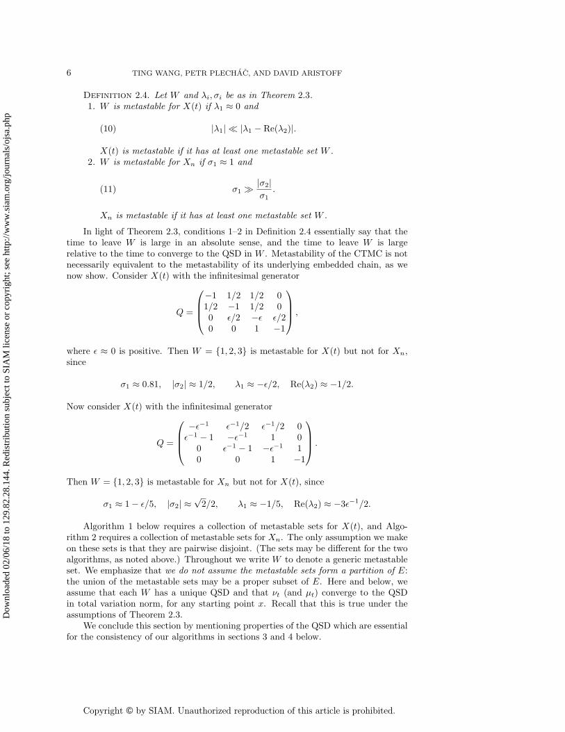
Definition 2.4. Let W and λi, σi be as in Theorem 2.3.1. W is metastable for X(t) if λ1 ≈ 0 and

(10) |λ1| � |λ1 − Re(λ2)|.

X(t) is metastable if it has at least one metastable set W .2. W is metastable for Xn if σ1 ≈ 1 and

(11) σ1 �|σ2|σ1

.

Xn is metastable if it has at least one metastable set W .

In light of Theorem 2.3, conditions 1–2 in Definition 2.4 essentially say that thetime to leave W is large in an absolute sense, and the time to leave W is largerelative to the time to converge to the QSD in W . Metastability of the CTMC is notnecessarily equivalent to the metastability of its underlying embedded chain, as wenow show. Consider X(t) with the infinitesimal generator

Q =

−1 1/2 1/2 01/2 −1 1/2 00 ε/2 −ε ε/20 0 1 −1

,

where ε ≈ 0 is positive. Then W = {1, 2, 3} is metastable for X(t) but not for Xn,since

σ1 ≈ 0.81, |σ2| ≈ 1/2, λ1 ≈ −ε/2, Re(λ2) ≈ −1/2.

Now consider X(t) with the infinitesimal generator

Q =

−ε−1 ε−1/2 ε−1/2 0ε−1 − 1 −ε−1 1 0

0 ε−1 − 1 −ε−1 10 0 1 −1

.

Then W = {1, 2, 3} is metastable for Xn but not for X(t), since

σ1 ≈ 1− ε/5, |σ2| ≈√

2/2, λ1 ≈ −1/5, Re(λ2) ≈ −3ε−1/2.

Algorithm 1 below requires a collection of metastable sets for X(t), and Algo-rithm 2 requires a collection of metastable sets for Xn. The only assumption we makeon these sets is that they are pairwise disjoint. (The sets may be different for the twoalgorithms, as noted above.) Throughout we write W to denote a generic metastableset. We emphasize that we do not assume the metastable sets form a partition of E:the union of the metastable sets may be a proper subset of E. Here and below, weassume that each W has a unique QSD and that νt (and µt) converge to the QSDin total variation norm, for any starting point x. Recall that this is true under theassumptions of Theorem 2.3.

We conclude this section by mentioning properties of the QSD which are essentialfor the consistency of our algorithms in sections 3 and 4 below.

Dow

nloa

ded

02/0

6/18

to 1

29.8

2.28

.144

. Red

istr

ibut

ion

subj

ect t

o SI

AM

lice

nse

or c

opyr

ight

; see

http

://w

ww

.sia

m.o

rg/jo

urna

ls/o

jsa.

php



Theorem 2.5.1. Suppose X(0) ∼ ν. Then T is exponentially distributed with the parameter−λ1:

Pν(T > t) = eλ1t, t > 0,

and T and X(T ) are independent.2. Suppose X0 ∼ µ. Then N is geometrically distributed with the parameter

1− σ1:Pµ(N > n) = σn1 , n = 1, 2, . . . ,

and N and XN are independent.

Proof. The first part of 1 and 2 was shown in Theorem 2.3. For the rest of theproof, see [6].

3. The CTMC ParRep method.

3.1. Formulation of the CTMC algorithm. In this section, we introduce amethod for accelerating the computation of π(f), where we recall f : E → R is anybounded function and π is the stationary distribution. We call this algorithm, CTMCParRep, for reasons that will be outlined below. Before we describe CTMC ParRep,we introduce some notation. Throughout, X1(t), . . . , XR(t) will be independent pro-cesses with the same law as X(t) and with initial distributions supported in W . Recallthat the first exit time of X(t) from W is

T = inf{t > 0 : X(t) /∈W}.

Similarly, for r = 1, . . . , R, we define the first exit time of Xr(t) from W by

T r = inf{t > 0 : Xr(t) /∈W}

and the smallest one among them by

T ∗ = minrT r.

We denote the index of the replica with the first exit time T ∗ by M , i.e.,

M = arg minr

T r.

T , T r, T ∗, and M depend on W , but we do not make this explicit.We are in the position to present the CTMC ParRep in Algorithm 1. In this

algorithm, we will need user-chosen parameters tc associated with each metastable setW . Roughly speaking, these parameters correspond to the time forX(t) to converge tothe QSD inW . The accumulated value F (f)sim serves as a quantity that approximatesthe integral

∫ Tend

0 f(X(s)) ds when the algorithm terminates. Note that at the end ofthe algorithm we often have Tsim ≥ Tend since the ParRep process could reach Tendduring the parallel stage. However, this is not an issue as long as Tsim is large enoughat the end of the algorithm so that the time average is well approximated.

If Xpar(t) remains in W for a sufficiently long time (i.e., decorrelation thresholdtc), it is distributed nearly according to the QSD ν of X(t) in W by Theorem 2.3.This means that at the end of the decorrelation stage, Xpar(Tsim) can be considereda sample of ν.

The aim of the dephasing stage is to prepare a sequence of independent initialstates with distribution ν. There are several ways to achieve this. Perhaps the

Dow

nloa

ded

02/0

6/18

to 1

29.8

2.28

.144

. Red

istr

ibut

ion

subj

ect t

o SI

AM

lice

nse

or c

opyr

ight

; see

http

://w

ww

.sia

m.o

rg/jo

urna

ls/o

jsa.

php



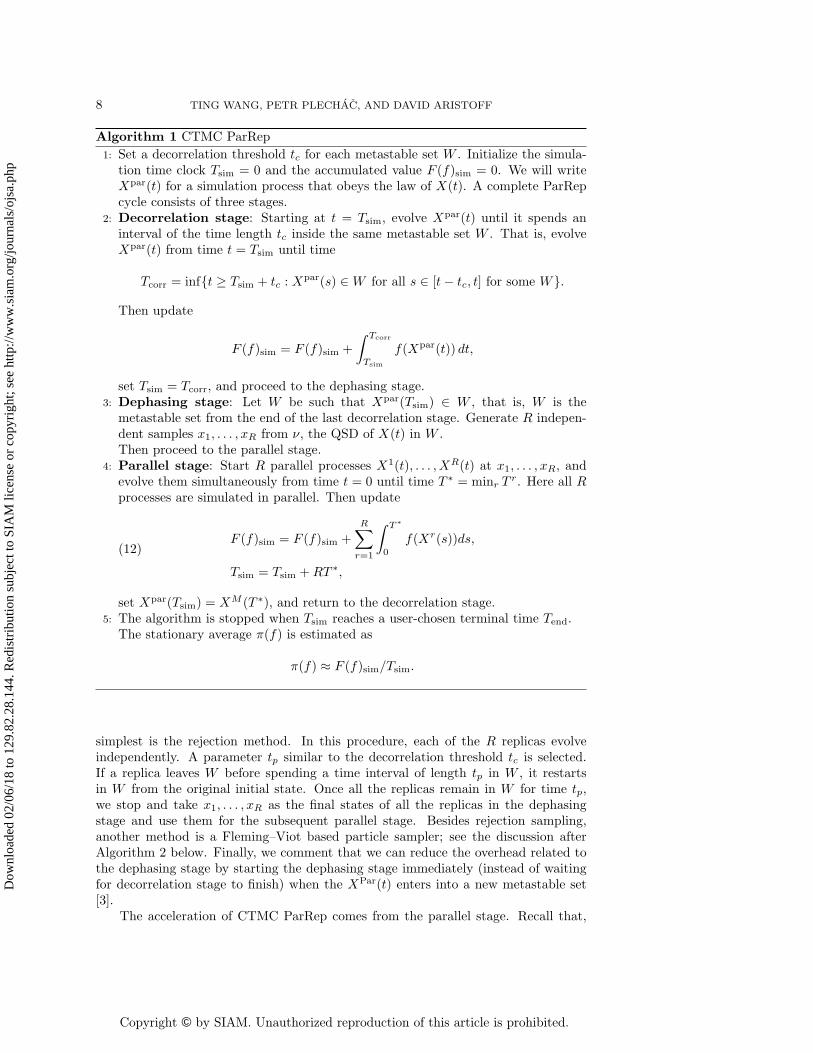
Algorithm 1 CTMC ParRep1: Set a decorrelation threshold tc for each metastable set W . Initialize the simula-

tion time clock Tsim = 0 and the accumulated value F (f)sim = 0. We will writeXpar(t) for a simulation process that obeys the law of X(t). A complete ParRepcycle consists of three stages.

2: Decorrelation stage: Starting at t = Tsim, evolve Xpar(t) until it spends aninterval of the time length tc inside the same metastable set W . That is, evolveXpar(t) from time t = Tsim until time

Tcorr = inf{t ≥ Tsim + tc : Xpar(s) ∈W for all s ∈ [t− tc, t] for some W}.

Then update

F (f)sim = F (f)sim +∫ Tcorr

Tsim

f(Xpar(t)) dt,

set Tsim = Tcorr, and proceed to the dephasing stage.3: Dephasing stage: Let W be such that Xpar(Tsim) ∈ W , that is, W is the

metastable set from the end of the last decorrelation stage. Generate R indepen-dent samples x1, . . . , xR from ν, the QSD of X(t) in W .Then proceed to the parallel stage.

4: Parallel stage: Start R parallel processes X1(t), . . . , XR(t) at x1, . . . , xR, andevolve them simultaneously from time t = 0 until time T ∗ = minr T r. Here all Rprocesses are simulated in parallel. Then update

F (f)sim = F (f)sim +R∑r=1

∫ T∗

0f(Xr(s))ds,

Tsim = Tsim +RT ∗,

(12)

set Xpar(Tsim) = XM (T ∗), and return to the decorrelation stage.5: The algorithm is stopped when Tsim reaches a user-chosen terminal time Tend.

The stationary average π(f) is estimated as

π(f) ≈ F (f)sim/Tsim.

simplest is the rejection method. In this procedure, each of the R replicas evolveindependently. A parameter tp similar to the decorrelation threshold tc is selected.If a replica leaves W before spending a time interval of length tp in W , it restartsin W from the original initial state. Once all the replicas remain in W for time tp,we stop and take x1, . . . , xR as the final states of all the replicas in the dephasingstage and use them for the subsequent parallel stage. Besides rejection sampling,another method is a Fleming–Viot based particle sampler; see the discussion afterAlgorithm 2 below. Finally, we comment that we can reduce the overhead related tothe dephasing stage by starting the dephasing stage immediately (instead of waitingfor decorrelation stage to finish) when the XPar(t) enters into a new metastable set[3].

The acceleration of CTMC ParRep comes from the parallel stage. Recall that,

Dow

nloa

ded

02/0

6/18

to 1

29.8

2.28

.144

. Red

istr

ibut

ion

subj

ect t

o SI

AM

lice

nse

or c

opyr

ight

; see

http

://w

ww

.sia

m.o

rg/jo

urna

ls/o

jsa.

php



for each r = 1, . . . , R, if x1, . . . , xR are independent, identically distributed (iid) withthe common distribution ν, then T 1, . . . , TR are independent exponential randomvariables with common parameter λ1. Using T ∗ = minr T r, it is then easy to checkthat RT ∗ has the same distribution as T 1. See Lemma 3.1 below. This meansone need only wait for T ∗ instead of T 1 to observe an exit from W . Note thatthis is true whether or not W is metastable, so efficiency of the parallel stage doesnot require metastability. However, the dephasing stage is not efficient if W is notmetastable. That is because, in practice, the samples x1, . . . , xR are obtained bysimulating trajectories which remain in W for a sufficiently long time tp. Such samplesare hard to obtain when the typical time tp for x1, . . . , xR to reach the QSD in W isnot much smaller than the typical time to leave W .

To see that each parallel stage has a consistent contribution to the stationaryaverage, we make the following two observations. Suppose that x1, . . . , xR are iidsamples from ν.

1. The joint law of (RT ∗, XM (T ∗)) is the same as that of (T 1, X(T 1)). That is,the joint distribution of the first exit time and the exit state in the parallelstage is independent of the number of replicas.

2. The expected value of∑Rr=1

∫ T∗

0 f(Xr(s))ds in (12) is the same as that of∫ T 1

0 f(X1(s))ds. That is, the expected contribution to F (f)sim from eachparallel stage is independent of the number of replicas.

The first observation is a consequence of Theorem 2.5, and the second will be proved inTheorem 3.2 below. Consistency of stationary averages follows from points 1–2 aboveand the law of large numbers. Since there are indefinitely many parallel stages in agiven W , consistency is ensured as long as the expected contribution to F (f)sim fromthe parallel stage has the correct expected value. See [1] for details and discussion ina related discrete time version of the algorithm under some idealized assumptions.

The CTMC ParRep algorithm suffers some serious drawbacks. Even if the parallelprocessors are synchronous, M and T ∗ may not be known at the wall clock time whenthe first replica leaves W . The reason is that the holding times for a CTMC arerandom, while the wall clock time for simulating each jump of the CTMC is alwaysroughly the same. We illustrate this problem in Figure 1. In the worst possiblecase, in order to determine M and T ∗, we must wait for all the replicas to leaveW . However, one can set a variable Tmin to record the current minimum first exittime over all replicas which have left W , and terminate any replicas which reach timeTmin but have not left W , since no replica contributes to the accumulated value pasttime Tmin. Since the expected first exit times E[T r], r = 1, . . . , R, are roughly thesame, if the variance in the number of jumps of Xr(t) before time T ∗ is small for allr = 1, . . . , R, then we can expect that the parallel stage stops after only a few replicasleave W .

For the same reason, there is another major drawback of CTMC ParRep. If ftakes multiple values in W , then the computation of

∑Rr=1

∫ T∗

0 f(Xr(s))ds in (12)requires storing the entire history of the value of f on each replica in that parallelstage. We illustrate this drawback by considering the case of two replicas r1 and r2with first exit time T 1 and T 2, respectively. Suppose T 1 < T 2 and hence T ∗ = T 1.Let us assume that in terms of wall clock time, r2 exits W before r1 does. At the endof the parallel stage (i.e., after both of T 1 and T 2 are sampled) we have the running

sum∫ T 2

0 f(X2(s))ds from r2. However, by the CTMC ParRep algorithm, we only

need∫ T∗

0 f(X2(s))ds indeed. If we only keep track of the running sum, we are unable

Dow

nloa

ded

02/0

6/18

to 1

29.8

2.28

.144

. Red

istr

ibut

ion

subj

ect t

o SI

AM

lice

nse

or c

opyr

ight

; see

http

://w

ww

.sia

m.o

rg/jo

urna

ls/o

jsa.

php



1

2

0 1 2 2.5 4 5 6 7

0 1 1.5 4 8

Fig. 1. The parallel stage of the CTMC ParRep algorithm with two replicas. R1 escapes fromW at t = 7 with seven transitions while R2 escapes at t = 8 but with only four transitions. In theparallel stage of the CTMC ParRep algorithm, R2 escaped from W before R1 does but T 2 > T 1.There is no acceleration in this case since the parallel stage does not terminate when R2 escapes.

to recover∫ T∗

0 f(X2(s))ds from T 2. Hence, the implementation of the CTMC ParRepmight be memory demanding unless one is interested in the equilibrium average of ametastable-set invariant function f , i.e., if f(x) has only one value in each metastableset W . In section 4 we present another algorithm, called embedded ParRep, whichaddresses these drawbacks.

3.2. Error analysis of CTMC ParRep. Here and below we will write EνR

for the expectation of (X1(t), . . . , XR(t)) starting at νR, where for

νR(x1, . . . , xR) =R∏r=1

ν(xr), x1, . . . , xR ∈W.

We begin with a simple well-known lemma.

Lemma 3.1. Suppose T 1, . . . , TR are iid exponential random variables with theparameter λ1. Then T ∗ = min1≤r≤R T

r is exponentially distributed with the parameterRλ1. In particular, RT ∗ has the same distribution as T 1.

We now show that if the dephasing sampling is exact, then the expected con-tribution to the accumulated value F (f)sim from the parallel step of Algorithm 1 isexact.

Theorem 3.2. Suppose in the dephasing step (x1, . . . , xR) ∼ νR. Then the ex-pected contribution to F (f)sim from the parallel stage of Algorithm 1 is independentof the number of replicas,

EνR

[R∑r=1

∫ T∗

0f(Xr(s))ds

]= Eν

[∫ T

0f(X(s))ds

]= ν(f)Eν [T ].

Proof. First we consider the case with a single replica. We condition on the exittime T 1 and write

Eν[∫ T 1

0f(X1(s))ds

]=∫ ∞

0Eν[∫ t

0f(X1(s))ds

∣∣∣∣T 1 = t

]Pν(T 1 ∈ dt).

Interchanging the two integrals of the right-hand side leads to∫ ∞0

∫ ∞s

Eν[f(X1(s))|T 1 = t

]P(T 1 ∈ dt)ds.

Dow

nloa

ded

02/0

6/18

to 1

29.8

2.28

.144

. Red

istr

ibut

ion

subj

ect t

o SI

AM

lice

nse

or c

opyr

ight

; see

http

://w

ww

.sia

m.o

rg/jo

urna

ls/o

jsa.

php



Note that the inner integral can be written as Eν[f(X1(s))1T 1>s

]and hence

Eν[∫ T 1

0f(X1(s))ds

]=∫ ∞

0Eν[f(X1(s))|T 1 > s

]Pν(T 1 > s)ds.

Owing to the definition of QSD and the fact that Eν [T 1] =∫∞

0 Pν(T 1 > s)ds,

Eν[∫ T 1

0f(X1(s))ds

]= ν(f)Eν [T 1].

In the case of multiple replicas, similar steps can be used to show that

R∑r=1

EνR

[∫ T∗

0f(Xr(s))ds

]=

R∑r=1

∫ ∞0

EνR

[f(Xr(s))|T ∗ > s] PνR

(T ∗ > s)ds.

Recall that T ∗ > s if and only if T r > s for all r = 1, . . . , R. Using this, the fact thatT 1, . . . , T r are independent, and the definition of the QSD, we get

EνR

[f(Xr(s))|T ∗ > s] = Eν [f(Xr(s))|T r > s] = ν(f).

ThusR∑r=1

EνR

[∫ T∗

0f(Xr(s))ds

]= ν(f)

R∑r=1

∫ ∞0

PνR

(T ∗ > s)ds = ν(f)REνR

[T ∗].

Finally, the result follows from Lemma 3.1.

The purpose of CTMC ParRep is to efficiently simulate very long trajectories ofa metastable CTMC and estimate the equilibrium average π(f). CTMC ParRep canproduce accelerated dynamics of the CTMC on a coarse state space where each coarseset corresponds to some W ; see the discussion below Algorithm 2 below. Our numer-ical experiments suggest that CTMC ParRep (and also embedded ParRep describedbelow) are consistent for estimating the stationary distribution.

For CTMC ParRep, we justify this claim in Theorem 3.3 below, which shows that,starting in some W and waiting until the simulation leaves W , the error for a completeParRep cycle in CTMC ParRep compared to direct (serial) simulation vanishes as tcincreases. See Theorem 4.4 below for the analogous result on embedded ParRep. Wenote that each ParRep cycle produce an error in the estimation of stationary averagesthat does not disappear as Tsim → ∞. However, we expect that the error vanishesas the thresholds tc = tp → ∞. Study of this error is more involved and will be thefocus of another work.

Recall we have assumed convergence of ‖νtc − ν‖TV → 0 as tc → ∞, for everystarting point x ∈ E, where ‖·‖TV denotes total variation norm; see, for instance, The-orem 2.3 for conditions guaranteeing this convergence.

Theorem 3.3. Consider CTMC ParRep starting at x ∈ W in the decorrelationstage. Assume the dephasing stage sampling is exact, that is, (x1, . . . , xR) ∼ νR.Consider the expected contribution to F (f)sim until the first time the simulation leavesW (either in the decorrelation or in the parallel stage),

∆F (f)sim , Ex[∫ tc∧T

0f(X(s)) ds

]+ Ex,ν

R

[1T>tc

R∑r=1

∫ T∗

0f(Xr(s))ds

],

Dow

nloa

ded

02/0

6/18

to 1

29.8

2.28

.144

. Red

istr

ibut

ion

subj

ect t

o SI

AM

lice

nse

or c

opyr

ight

; see

http

://w

ww

.sia

m.o

rg/jo

urna

ls/o

jsa.

php



where Ex,νR

denotes expectation for (X(t), X1(t), . . . , XR(t)) with X(t) starting atx and the replicas (X1(t), . . . , XR(t)) starting at initial distribution νR. The errorcompared to direct (serial) simulation satisfies the bound

(13)

∣∣∣∣∣Ex[∫ T

0f(X(s))ds

]−∆F (f)sim

∣∣∣∣∣ ≤ ‖f‖∞ supx∈W

Ex [T ] ‖νtc − ν‖TV.

Proof. We estimate∣∣∣∣∣Ex[∫ T

0f(X(s))ds

]−∆F (f)sim

∣∣∣∣∣=

∣∣∣∣∣Ex[∫ T

tc∧Tf(X(s))ds

]− Ex,ν

R

[1T>tc

R∑r=1

∫ T∗

0f(Xr(s))ds

]∣∣∣∣∣=

∣∣∣∣∣Ex[∫ T

tc

f(X(s))ds

∣∣∣∣∣ T > tc

]− Ex,ν

R

[R∑r=1

∫ T∗

0f(Xr(s))ds

∣∣∣∣∣ T > tc

]∣∣∣∣∣Px(T > tc)

≤

∣∣∣∣∣Ex[∫ T

tc

f(X(s))ds

∣∣∣∣∣ T > tc

]− Eν

R

[R∑r=1

∫ T∗

0f(Xr(s))ds

]∣∣∣∣∣ ,where we used the fact that X(t) and the replicas (X1(t), . . . , XR(t)) are independent.By the Markov property,

Ex[∫ T

tc

f(X(s))ds

∣∣∣∣∣ T > tc

]= Eνtc

[∫ T

0f(X(s))ds

].

By Theorem 3.2,

EνR

[R∑r=1

∫ T∗

0f(Xr(s))ds

]= Eν

[∫ T

0f(X(s)) ds

].

Combining the above estimates and equalities,∣∣∣∣∣Ex[∫ T

0f(X(s))ds

]−∆F (f)sim

∣∣∣∣∣≤

∣∣∣∣∣Eνtc

[∫ T

0f(X(s))ds

]− Eν

[∫ T

0f(X(s)) ds

]∣∣∣∣∣=

∣∣∣∣∣∑x∈W

Ex[∫ T

0f(X(s))ds

]νtc(x)−

∑x∈W

Ex[∫ T

0f(X(s))ds

]ν(x)

∣∣∣∣∣≤‖f‖∞ sup

x∈WEx [T ] ‖νtc − ν‖TV.

We note that Ex[T ] is uniformly bounded in x ∈ W if, for instance, PW is irre-ducible and W is finite and nonabsorbing for X(t), as in Theorem 2.3. This uniformboundedness guarantees that the right-hand side of (13) vanishes as tc →∞.

Dow

nloa

ded

02/0

6/18

to 1

29.8

2.28

.144

. Red

istr

ibut

ion

subj

ect t

o SI

AM

lice

nse

or c

opyr

ight

; see

http

://w

ww

.sia

m.o

rg/jo

urna

ls/o

jsa.

php



4. The embedded ParRep method.

4.1. Formulation of the embedded ParRep algorithm. In this section, weintroduce another algorithm for accelerating the computation of π(f). The algorithm,called embedded ParRep, circumvents the disadvantages of CTMC ParRep discussedabove. As mentioned in the previous section, CTMC ParRep can be slow due tothe randomness of the holding times. In the worst case, one has to wait until allreplicas leave W in order to determine the first exit time T ∗. To circumvent this issuewe propose an algorithm based on the embedded chain in which the parallel stageterminates as soon as one of the replicas leaves W .

Before we describe embedded ParRep, we introduce some notation. Throughout,X1n, . . . , X

Rn will be independent processes with the same law as Xn and with initial

distributions supported in W . Moreover, we consider X1n, . . . , X

Rn as the embedded

chains of X1(t), . . . , Xr(t) defined above, and let ∆τ1n, . . . ,∆τ

Rn be the corresponding

holding times. Recall that the first exit time of Xn from W is

N = inf{n > 0 : Xn /∈W}.

For r = 1, . . . , R, we define the first exit time of Xrn from W by

Nr = min{n ∈ N;Xrn /∈W}

and the smallest among them by

N∗ = min{Nr; r = 1, . . . , R}.

Note that it is possible that more than one replica leave W for the first time after N∗

transitions. We denote by K the smallest index among these escaped replicas. Thatis,

K = min{r = 1, . . . , R;XrN∗ /∈W}.

It is clear from the above definition that NK = N∗. Of course N , Nr, N∗, and Kdepend on W , but we do not make this explicit.

Here and below we write EµR

for expectation of (X1n, . . . , X

Rn ) starting at µR,

where

µR(x1, . . . , xR) =R∏r=1

µ(xr), x1, . . . , xR ∈W.

We begin by reproducing from [2] Theorems 4.1 and 4.2 below, with proofs for com-pleteness.

Theorem 4.1. Suppose (X1n, . . . , X

Rn ) has initial distribution µR. Then R(NK−

1) +K has the same distribution as N1.

Proof. Note that for any n ≥ 0 and k = 1, . . . , R, the event {NK = n,K = k}is equivalent to the event {N1 > n, . . . , Nk−1 > n,Nk = n,Nk+1 > n− 1, . . . , NR >n − 1}. Since X1

n, . . . , XRn are iid and N1 is geometrically distributed with rate

p = PµR

(N1 > 1) (see Theorem 2.5),

PµR

(NK = n,K = k) = (1−p)n(k−1)(1−p)n−1p(1−p)(n−1)(k−1) = (1−p)R(n−1)+k−1p.

That is, R(NK − 1) +K has geometric distribution with rate p.

Dow

nloa

ded

02/0

6/18

to 1

29.8

2.28

.144

. Red

istr

ibut

ion

subj

ect t

o SI

AM

lice

nse

or c

opyr

ight

; see

http

://w

ww

.sia

m.o

rg/jo

urna

ls/o

jsa.

php



Theorem 4.2. Suppose (X1n, . . . , X

Rn ) has the initial distribution µR. Then XK

NK

is independent of R(NK − 1) +K and the distribution of (XKNK , R(NK − 1) +K) is

the same as that of (X1N1 , N1).

Proof. We first prove that XKNK is independent of K. Since XR

n , . . . , XRn are iid

and Nk is independent of XkNk for each k, then Xk

Nk is independent of N1, . . . , NR.Note that K ∈ σ(N1, . . . , NR), hence Xk

Nk is independent of K for each k. Nowobserve that for any A ⊂ E,

PµR

(XKNK ∈ A) =

R∑r=1

PµR

(XkNk ∈ A,K = r)

=R∑r=1

PµR

(X1N1 ∈ A)Pµ

R

(K = r)

= PµR

(X1N1 ∈ A),

that is, XKNK and X1

N1 are equally distributed. This implies that XKNK is independent

of K. To see the independence between XKNK and R(NK − 1) +K, note that

PµR

(XKNK ∈ A,NK = n,K = r) = Pµ

R

(XrNr ∈ A,Nr = n,K = r)

= PµR

(XrNr ∈ A,K = r|Nr = n)Pµ

R

(Nr = n)

= PµR

(XrNr ∈ A|Nr = n)Pµ

R

(Nr = n,K = r)

= PµR

(XrNr ∈ A)Pµ

R

(Nr = n,K = r)

= PµR

(XKNK ∈ A)Pµ

R

(NK = n,K = r)

for any measurable A ⊂ E, n ∈ Z+ and r = 1, . . . , R. Finally, Theorem 4.1 andthe above analysis imply that (XK

NK , R(NK − 1) + K) and (X1N1 , N1) are equally

distributed.

Now we present the embedded ParRep algorithm in Algorithm 2. In this algo-rithm we will need user-chosen parameters nc associated with each metastable set W .Roughly, these parameters correspond to the time for Xn to converge to the QSD inW .

The DTMC Xn and holding times ∆τn are simulated by the stochastic simulationalgorithm (SSA); see, for instance, [13], just as in the CTMC ParRep. If Xpar

n remainsin W for a sufficiently long time (i.e., time tc), it is distributed nearly according to theQSD µ of Xn in W . See Theorem 2.3. This means that at the end of the decorrelationstage, Xpar

n can be considered a sample of µ.The aim of the dephasing stage is to prepare a sequence of iid initial states

with distribution µ. Like the CTMC ParRep, rejection sampling can be used forthe embedded ParRep as well. However, a more natural and efficient option for theembedded ParRep is a Fleming–Viot based sampling procedure [3, 11]. The procedurecan be summarized as follows.

The R replicas X1n, . . . , X

Rn , starting in W , evolve until one or more of them leaves

W . Then each replica that left W is restarted from the current state of another replicathat is currently in W (usually chosen uniformly at random). The procedure stopsafter the replicas have evolved for n = np time steps, where np is a parameter similarto nc. (If all the replicas leave W at the same time, the procedure restarts from thebeginning.) With this type of sampling, the number of time steps simulated for each

Dow

nloa

ded

02/0

6/18

to 1

29.8

2.28

.144

. Red

istr

ibut

ion

subj

ect t

o SI

AM

lice

nse

or c

opyr

ight

; see

http

://w

ww

.sia

m.o

rg/jo

urna

ls/o

jsa.

php



Algorithm 2 Embedded ParRep1: Set a decorrelation threshold nc for each metastable set W . Initialize the sim-

ulation time clock Nsim = 0 and the accumulated value F (f)sim = 0. We willwrite Xpar

n and ∆parn for a DTMC and holding time process following the law of

the embedded chain and holding times of X(t), respectively. A complete ParRepcycle consists of three stages.

2: Decorrelation stage: Starting at n = Nsim, evolve Xparn and ∆τpar

n until Xparn

spends nc consecutive time steps inside of the same metastable set W . That is,evolve Xpar

n and ∆τparn from time n = Nsim until time

Ncorr = inf{n ≥ Nsim+nc−1 : Xparm ∈W for m ∈ {n−nc+1, . . . , n} for some W}.

Then update

F (f)sim = F (f)sim +Ncorr−1∑n=Nsim

f(Xparn )∆τpar

n ,

set Nsim = Ncorr, and proceed to the dephasing stage.3: Dephasing stage: Let W be such that Xpar

Nsim∈W , that is, W is the metastable

set from the end of the decorrelation stage. Generate R independent samplesx1, . . . , xR from µ, the QSD of Xn in W . Then proceed to the parallel stage.

4: Parallel stage: Start R parallel processes X1n, . . . , X

Rn at x1, . . . , xR, and evolve

them and the corresponding holding times ∆τ1n, . . . ,∆τ

Rn from time n = 0 until

time N∗. Then update

F (f)sim = F (f)sim +R∑r=1

N∗−2∑k=0

f(Xrk)∆τ rk +

K∑r=1

f(XrN∗−1)∆τ rN∗−1,

Nsim = Nsim +R(N∗ − 1) +K,

(14)

set XparNsim

= XKN∗ , and return to the decorrelation stage.

5: The algorithm is stopped when Nsim reaches some user-chosen time Nend. Thestationary average π(f) is estimated as

π(f) ≈ F (f)sim/F (1)sim.

replica in the dephasing step is the same. In particular, if the R parallel processorsare synchronous (i.e., if each processor takes the same wall clock time to simulateone time step), then each processor finishes the dephasing step at the same wall clocktime. We comment that the Fleming–Viot technique can be used to estimate thedecorrelation and dephasing thresholds as well when they are difficult to choose apriori [3].

The acceleration of the embedded ParRep comes from the parallel stage. Figure2 shows the diagram for the parallel stage with R replicas. Roughly, we only haveto wait N∗ time steps instead of N to observe an exit from W . The theoreticalwall clock time speedup can be approximately a factor of R. See Theorem 4.1 below.Similar to CTMC ParRep, the parallel step does not require metastability for this timespeedup, but if W is not metastable, then the dephasing step will not be efficient. See

Dow

nloa

ded

02/0

6/18

to 1

29.8

2.28

.144

. Red

istr

ibut

ion

subj

ect t

o SI

AM

lice

nse

or c

opyr

ight

; see

http

://w

ww

.sia

m.o

rg/jo

urna

ls/o

jsa.

php



0

0

0

0

0

=R1

=R!11

= 31

= 21

= 11

=RN$

=R!1N$

= 3N$

= 2N$

= 1N$

=RN$!1

=R!1N$!1

= 3N$!1

= 2N$!1

= 1N$!1

R

R! 1

3

2

1

Fig. 2. The diagram for one parallel stage of the embedded ParRep algorithm with R replicas.Each blue dot represents an exit event along the time line. Both replica 2 and 3 leave W afterN∗ = 6 transitions (the blue dot with the red “x”), in which case K = 2. (Figure is in color online.)

the remarks below Algorithm 1.Similar to the CTMC ParRep, each parallel stage of the embedded ParRep has a

consistent averaged contribution to the stationary average. Suppose that x1, . . . , xRare iid samples from µ.

1. The joint law of (XKNK , R(NK − 1) + K) is the same as that of (X1

N1 , N1).That is, the joint distribution of the first exit time and the exit state for eachparallel stage is independent of the number of replicas.

2. The expected value of

R∑r=1

N∗−2∑k=0

f(Xrk)∆τ rk +

K∑r=1

f(XrN∗−1)∆τ rN∗−1

is the same as that ofN−1∑n=0

f(X1n)∆τ1

n.

Hence the expected contribution to F (f)sim from each parallel stage is inde-pendent of the number of replicas. See Theorem 4.3 below.

See Theorems 4.2 and 4.3 for proofs of these statements.We expect that embedded ParRep is superior to the CTMC ParRep for the fol-

lowing two reasons. First, consider the parallel stages of both algorithms. In theCTMC ParRep, observing the first exit event in the parallel stage is not sufficient todetermine T ∗. But in embedded ParRep, once any replica leaves W , we know N∗.Thus the embedded ParRep parallel step terminates once any of the replicas leavesW . For this reason we expect the parallel stage of the embedded ParRep to be signif-icantly faster than that of the CTMC ParRep. Second, consider the dephasing stage.For the embedded ParRep, Fleming–Viot sampling is a natural technique because ifthe processors are synchronous, then they all finish the dephasing stage at the samewall clock time, and only the current states of each processor are needed at each timestep to decide where to restart replicas which left W . For asynchronous processors,

Dow

nloa

ded

02/0

6/18

to 1

29.8

2.28

.144

. Red

istr

ibut

ion

subj

ect t

o SI

AM

lice

nse

or c

opyr

ight

; see

http

://w

ww

.sia

m.o

rg/jo

urna

ls/o

jsa.

php



one can simply implement a polling time. This is not true, however, for Fleming–Viotsampling with the CTMC ParRep. Indeed, to implement Fleming–Viot samplingwith the CTMC ParRep, one would have to store the histories of every replica, andthe replicas would finish at potentially very different wall clock times. The rejectionmethod can be slow for both algorithms, particularly when the metastability is weakor when the number of replicas is large.

4.2. Error analysis of the embedded ParRep. Now we are able to showthat if the dephasing sampling is exact, then the expected contribution to F (f)simfrom the parallel stage is exact.

Theorem 4.3. Suppose in the dephasing step (x1, . . . , xR) ∼ µR. Then the ex-pected contribution to F (f)sim from the parallel stage of Algorithm 2 is the same forevery number of replicas.

EµR

[R∑r=1

N∗−2∑k=0

f(Xrk)∆τ rk +

K∑r=1


]= Eµ

[N−1∑n=0

f(Xn)∆τn

]= µ(fq−1)Eµ [N ] ,

where q is the function as defined in section 2.1.

Proof. We first rewrite

R∑r=1

N∗−2∑k=0

f(Xrk)∆τ rk +

K∑r=1


=R∑r=1

N∗−1∑i=0

f(Xri )∆τ ri −

R∑r=K+1

f(XrN∗−1)∆τ rN∗−1.

(15)

For the first part, we condition N∗ and obtain

EµR

[R∑r=1

N∗−1∑i=0

f(Xri )∆τ ri

]=

R∑r=1

∞∑n=1

n−1∑i=0

EµR

[f(Xri )∆τ ri IN∗=n] .

Interchanging the iterated summations leads toR∑r=1

∞∑n=1

n−1∑i=0

EµR

[f(Xri )∆τ ri IN∗=n] =

R∑r=1

∞∑i=0

EµR

[f(Xri )IN∗>i∆τ ri ] .

Notice N∗ > i is equivalent to N1 > i, . . . , NR > i and ∆τ ri is independent of Ns fors 6= r. Thus

R∑r=1

∞∑i=0

EµR

[f(Xri )∆τ ri |N∗ > i] Pµ

R

(N∗ > i)

=R∑r=1

∞∑i=0

EµR

[f(Xri )∆τ ri |Nr > i] Pµ

R

(N∗ > i).

Now by Lemma 2.1 and the definition of the QSD,

Eµ [f(Xri )∆τ ri |Nr > i] = Eµ [Eµ [f(Xr

i )∆τ ri | {Xrn}n=0,1,...]|Nr > i]

= Eµ [f(Xri )Eµ [∆τ ri | {Xr

n}n=0,1,...]|Nr > i]

= Eµ[f(Xr

i )q(Xri )−1

∣∣Nr > i]

= µ(fq−1).

Dow

nloa

ded

02/0

6/18

to 1

29.8

2.28

.144

. Red

istr

ibut

ion

subj

ect t

o SI

AM

lice

nse

or c

opyr

ight

; see

http

://w

ww

.sia

m.o

rg/jo

urna

ls/o

jsa.

php



Combining the last four equations gives

(16) EµR

[R∑r=1

N∗−1∑i=0

f(Xri )∆τ ri

]= µ(fq−1)REµ

R

[N∗].

A similar argument can be applied to the second term on the right-hand side of(15). First we condition N∗ and K simultaneously such that

EµR

[R∑

r=K+1


]

=∞∑n=1

R∑r=1

R∑r=k+1

EµR [f(Xr

n−1)∆τ rn−1|N∗ = n,K = k]Pµ

R

(N∗ = n,K = k).

Interchanging the second and third summations the right-hand side equals∞∑n=1

R∑r=2

r−1∑k=1

EµR [f(Xr

n−1)∆τ rn−1|N∗ = n,K = k]Pµ

R

(N∗ = n,K = k).

Recall that

N∗ = n, K = k ⇐⇒ N1 > n, . . . , Nk−1 > n, Nk = n, Nk+1 > n−1, . . . , NR > n−1.

Thus, using independence of X1n, . . . , X

Rn and the definition of the QSD,

∞∑n=1

R∑r=2

r−1∑k=1

EµR [f(Xr

n−1)∆τ rn−1|N∗ = n,K = k]Pµ

R

(N∗ = n,K = k)

=∞∑n=1

R∑r=2

r−1∑k=1

Eµ[f(Xr

n−1)∆τ rn−1|Nr > n− 1]Pµ

R

(N∗ = n,K = k)

=µ(fq−1)∞∑n=1

R∑r=2

r−1∑k=1

PµR

(N∗ = n,K = k)

=µ(fq−1)(R− EµR

[K]).

Combining the last three equations leads to

(17) Eµ[

R∑r=K+1


]= µ(fq−1)(R− Eµ

R

[K]).

Subtracting (17) from (16), we have

EµR

[R∑r=1

N∗−1∑i=0

f(Xri )∆τ ri −

R∑r=K+1


]= µ(fq−1)Eµ

R

[R(N∗ − 1) +K] .

Now the result follows since

µ(fq−1)EµR

[R(N∗ − 1) +K] = µ(fq−1)Eµ[N ]

by Theorem 4.2. In particular, when R = 1 we have N∗ = N and K = 1, and thus

Eµ[N−1∑n=0

f(Xn)∆τn

]= µ(fq−1)Eµ[N ].

Dow

nloa

ded

02/0

6/18

to 1

29.8

2.28

.144

. Red

istr

ibut

ion

subj

ect t

o SI

AM

lice

nse

or c

opyr

ight

; see

http

://w

ww

.sia

m.o

rg/jo

urna

ls/o

jsa.

php



We now prove an analog of Theorem 3.3 for the embedded ParRep. Recall wehave assumed convergence of ‖µnc

− µ‖TV → 0 as nc → ∞, for every starting pointx ∈ E. See, for instance, Theorem 2.3 for conditions guaranteeing this convergence.

Theorem 4.4. Consider the embedded ParRep starting at x ∈W in the decorrela-tion stage. Assume the dephasing stage sampling is exact, that is, (x1, . . . , xR) ∼ µR.Consider the expected contribution to F (f)sim up until the first time the simulationleaves W (either in the decorrelation stage or in the parallel stage):

∆F (f)sim , Ex[nc∧N−1∑n=0

f(Xn)∆τn

]+ Ex,µ

R

[1N>nc

R∑r=1

N∗−2∑k=0

f(Xrk)∆τ rk

+ 1N>nc

K∑r=1


],

where Ex,µR

denotes expectation for (Xn, X1n, . . . , X

Rn ) with Xn starting at x and the

replicas (X1n, . . . , X

Rn ) starting at the initial distribution µR. The error compared to

a direct (serial) simulation satisfies the bound

(18)

∣∣∣∣∣Ex[N−1∑n=0

f(Xn)∆τn

]−∆F (f)sim

∣∣∣∣∣ ≤ ‖f‖∞ supx∈W

Ex [T ] ‖µnc − µ‖TV.

Proof. The proof is similar to that for the CTMC ParRep,∣∣∣∣∣Ex[N−1∑n=0

f(Xn)∆τn

]−∆F (f)sim

∣∣∣∣∣=

∣∣∣∣∣Ex[

N−1∑n=nc∧N

f(Xn)∆τn

]− Ex,µ

R

[1N>nc

R∑r=1

N∗−2∑k=0

f(Xrk)∆τ rk

+ 1N>nc

K∑r=1


]∣∣∣∣∣≤

∣∣∣∣∣Ex[N−1∑n=nc

f(Xn)∆τn

∣∣∣∣∣N > nc

]

− EµR

[R∑r=1

N∗−2∑k=0

f(Xrk)∆τ rk +

K∑r=1


]∣∣∣∣∣ .By the Markov property

Ex[N−1∑n=nc

f(Xn)∆τn

∣∣∣∣∣N > nc

]= Eµnc

[N−1∑n=0

f(Xn)∆τn

].

Owing to Theorem 4.3,

EµR

[R∑r=1

N∗−2∑k=0

f(Xrk)∆τ rk +

K∑r=1


]= Eµ

[N−1∑n=0

f(Xn)∆τn

].

Dow

nloa

ded

02/0

6/18

to 1

29.8

2.28

.144

. Red

istr

ibut

ion

subj

ect t

o SI

AM

lice

nse

or c

opyr

ight

; see

http

://w

ww

.sia

m.o

rg/jo

urna

ls/o

jsa.

php



Therefore,∣∣∣∣∣Ex[N−1∑n=0

f(Xn)∆τn

]−∆F (f)sim

∣∣∣∣∣≤

∣∣∣∣∣Eµnc

[N−1∑n=0

f(Xn)∆τn

]− Eµ

[N−1∑n=0

f(Xn)∆τn

]∣∣∣∣∣=

∣∣∣∣∣∑x∈W

Ex[N−1∑n=0

f(Xn)∆τn

]µnc

(x)−∑x∈W

Ex[N−1∑n=0

f(Xn)∆τn

]µ(x)

∣∣∣∣∣≤ ‖f‖∞ sup

x∈WEx[T ]‖µnc

− µ‖TV

with the last equation coming from the fact that Ex[∑N−1n=0 ∆τn] = Ex[T ].

5. Numerical experiments. We present two numerical examples from thestochastic reaction networks in order to demonstrate the consistency and efficiency ofthe ParRep algorithms.

5.1. Reaction networks with linear propensity. We consider the followingstochastic reaction network:

(19) ∅ −→ A B −→ C −→ ∅

taken from [7], where A,B, and C represent reacting species. The time evolution ofthe population (the number of species) in the reaction network is commonly modeledas a CTMC X(t) = (X1(t), X2(t), X3(t)) with state space E ⊂ Z3

+. The jump rateof each reaction is governed by the propensity function (intensity) λj(x), j = 1, . . . , 5,such that for all t > 0,

λj(x) = limh→0

P(X(t+ h) = x+ ηj |X(t) = x)h

,

where ηj is the state change vector associated with the jth reaction. We list thereactions and their corresponding propensity functions and state change vectors inTable 1.

Table 1Reactions, propensity functions, and state change vectors.

Reaction Propensity function State change vector∅ −→ A λ1(x) = c1 η1 = (1, 0, 0)A −→ B λ2(x) = c2x1 η2 = (−1, 1, 0)B −→ A λ3(x) = c3x2 η3 = (1,−1, 0)B −→ C λ4(x) = c4x2 η4 = (0,−1, 1)C −→ ∅ λ5(x) = c5x3 η5 = (0, 0,−1)

In this numerical experiment, we take the initial state x0 = (5, 10, 10) and therate constants

(c1, c2, c3, c4, c5) = (0.1, 100, 100, 0.01, 0.01).

With this choice of parameters the timescale separation is about ε = 10−4 and hencethe process X(t) demonstrates metastability. The reactions A→ B and B → A occurwith a much higher probability than the other reactions and hence we call A→ B and

Dow

nloa

ded

02/0

6/18

to 1

29.8

2.28

.144

. Red

istr

ibut

ion

subj

ect t

o SI

AM

lice

nse

or c

opyr

ight

; see

http

://w

ww

.sia

m.o

rg/jo

urna

ls/o

jsa.

php



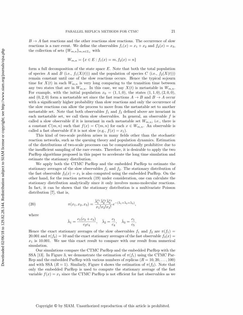
B → A fast reactions and the other reactions slow reactions. The occurrence of slowreactions is a rare event. We define the observables f1(x) = x1 + x2 and f2(x) = x3,the collection of sets {Wm,n}m,n∈Z+ with

Wm,n = {x ∈ E : f1(x) = m, f2(x) = n}

form a full decomposition of the state space E. Note that both the total populationof species A and B (i.e., f1(X(t))) and the population of species C (i.e., f2(X(t)))remain constant until one of the slow reactions occurs. Hence the typical sojourntime for X(t) in each Wm,n is very long comparing to the transition time betweenany two states that are in Wm,n. In this case, we say X(t) is metastable in Wm,n.For example, with the initial population x0 = (1, 1, 0), the states (1, 1, 0), (2, 0, 0),and (0, 2, 0) form a metastable set since the fast reactions A→ B and B → A occurwith a significantly higher probability than slow reactions and only the occurrence ofthe slow reactions can allow the process to move from the metastable set to anothermetastable set. Note that both observables f1 and f2 defined above are invariant ineach metastable set, we call them slow observables. In general, an observable f iscalled a slow observable if it is invariant in each metastable set Wm,n, i.e., there isa constant C(m,n) such that f(x) = C(m,n) for each x ∈ Wm,n. An observable iscalled a fast observable if it is not slow (e.g., f(x) = x1).

This kind of two-scale problem arises in many fields other than the stochasticreaction networks, such as the queuing theory and population dynamics. Estimationof the distributions of two-scale processes can be computationally prohibitive due tothe insufficient sampling of the rare events. Therefore, it is desirable to apply the twoParRep algorithms proposed in this paper to accelerate the long time simulation andestimate the stationary distribution.

We apply both the CTMC ParRep and the embedded ParRep to estimate thestationary averages of the slow observables f1 and f2. The stationary distribution ofthe fast observable f3(x) = x1 is also computed using the embedded ParRep. On theother hand, for the reaction network (19) under consideration, one can calculate thestationary distribution analytically since it only involves mono-molecular reactions.In fact, it can be shown that the stationary distribution is a multivariate Poissondistribution [7], that is,

(20) π(x1, x2, x3) =λx1

1 λx22 λx3

3

x1!x2!x3!e−(λ1+λ2+λ3),

where

λ1 =c1(c3 + c4)

c2c4, λ2 =

c1c4, λ3 =

c1c5.

Hence the exact stationary averages of the slow observables f1 and f2 are π(f1) =20.001 and π(f2) = 10 and the exact stationary averages of the fast observable f3(x) =x1 is 10.001. We use this exact result to compare with our result from numericalsimulation.

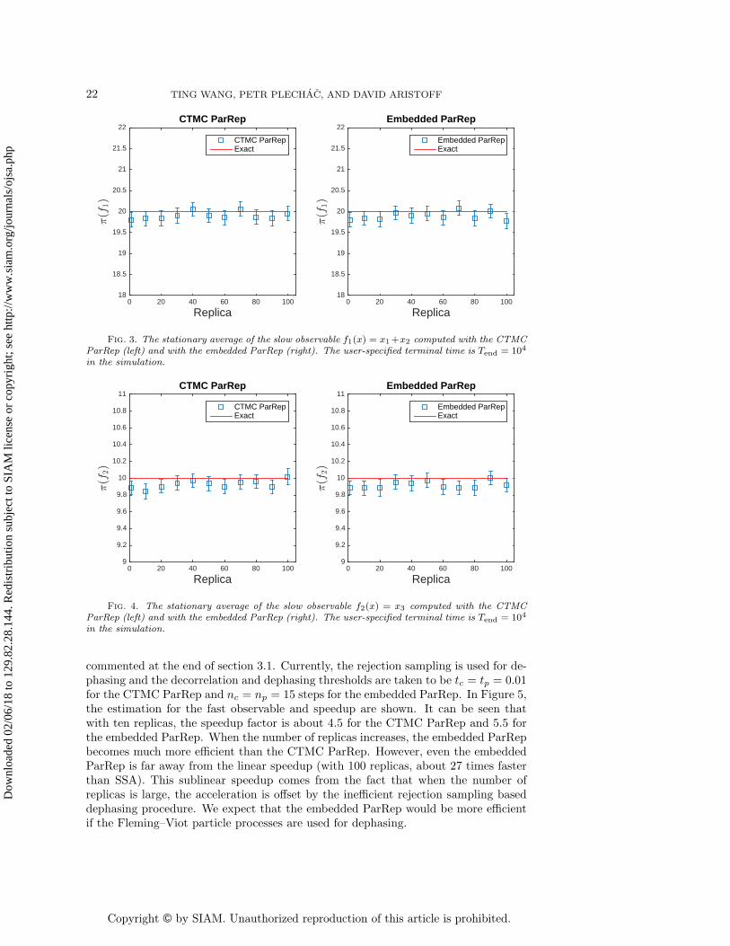
Our simulations compare the CTMC ParRep and the embedded ParRep with theSSA [13]. In Figure 3, we demonstrate the estimation of π(f1) using the CTMC Par-Rep and the embedded ParRep with various numbers of replicas (R = 10, 20, . . . , 100)and with SSA (R = 1). Similarly, Figure 4 shows the estimation of π(f2). Note thatonly the embedded ParRep is used to compute the stationary average of the fastvariable f(x) = x1 since the CTMC ParRep is not efficient for fast observables as we

Dow

nloa

ded

02/0

6/18

to 1

29.8

2.28

.144

. Red

istr

ibut

ion

subj

ect t

o SI

AM

lice

nse

or c

opyr

ight

; see

http

://w

ww

.sia

m.o

rg/jo

urna

ls/o

jsa.

php



Replica0 20 40 60 80 100

:(f

1)

18

18.5

19

19.5

20

20.5

21

21.5

22CTMC ParRep

CTMC ParRepExact

Replica0 20 40 60 80 100

:(f

1)

18

18.5

19

19.5

20

20.5

21

21.5

22Embedded ParRep

Embedded ParRepExact

Fig. 3. The stationary average of the slow observable f1(x) = x1+x2 computed with the CTMCParRep (left) and with the embedded ParRep (right). The user-specified terminal time is Tend = 104

in the simulation.

Replica0 20 40 60 80 100

:(f

2)

9

9.2

9.4

9.6

9.8

10

10.2

10.4

10.6

10.8

11CTMC ParRep

CTMC ParRepExact

Replica0 20 40 60 80 100

:(f

2)

9

9.2

9.4

9.6

9.8

10

10.2

10.4

10.6

10.8

11Embedded ParRep


Fig. 4. The stationary average of the slow observable f2(x) = x3 computed with the CTMCParRep (left) and with the embedded ParRep (right). The user-specified terminal time is Tend = 104

in the simulation.

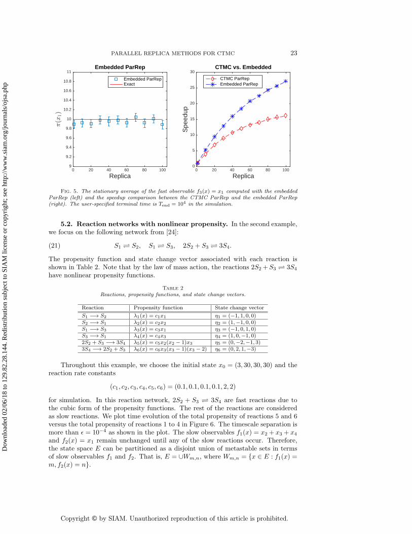
commented at the end of section 3.1. Currently, the rejection sampling is used for de-phasing and the decorrelation and dephasing thresholds are taken to be tc = tp = 0.01for the CTMC ParRep and nc = np = 15 steps for the embedded ParRep. In Figure 5,the estimation for the fast observable and speedup are shown. It can be seen thatwith ten replicas, the speedup factor is about 4.5 for the CTMC ParRep and 5.5 forthe embedded ParRep. When the number of replicas increases, the embedded ParRepbecomes much more efficient than the CTMC ParRep. However, even the embeddedParRep is far away from the linear speedup (with 100 replicas, about 27 times fasterthan SSA). This sublinear speedup comes from the fact that when the number ofreplicas is large, the acceleration is offset by the inefficient rejection sampling baseddephasing procedure. We expect that the embedded ParRep would be more efficientif the Fleming–Viot particle processes are used for dephasing.

Dow

nloa

ded

02/0

6/18

to 1

29.8

2.28

.144

. Red

istr

ibut

ion

subj

ect t

o SI

AM

lice

nse

or c

opyr

ight

; see

http

://w

ww

.sia

m.o

rg/jo

urna

ls/o

jsa.

php



Replica0 20 40 60 80 100

:(x

1)

9

9.2

9.4

9.6

9.8

10

10.2

10.4

10.6

10.8

11Embedded ParRep


Replica0 20 40 60 80 100

Spe

edup

0

5

10

15

20

25

30CTMC vs. Embedded

CTMC ParRepEmbedded ParRep

Fig. 5. The stationary average of the fast observable f3(x) = x1 computed with the embeddedParRep (left) and the speedup comparison between the CTMC ParRep and the embedded ParRep(right). The user-specified terminal time is Tend = 104 in the simulation.

5.2. Reaction networks with nonlinear propensity. In the second example,we focus on the following network from [24]:

(21) S1 S2, S1 S3, 2S2 + S3 3S4.

The propensity function and state change vector associated with each reaction isshown in Table 2. Note that by the law of mass action, the reactions 2S2 +S3 3S4have nonlinear propensity functions.

Table 2Reactions, propensity functions, and state change vectors.

Reaction Propensity function State change vectorS1 −→ S2 λ1(x) = c1x1 η1 = (−1, 1, 0, 0)S2 −→ S1 λ2(x) = c2x2 η2 = (1,−1, 0, 0)S1 −→ S3 λ3(x) = c3x1 η3 = (−1, 0, 1, 0)S3 −→ S1 λ4(x) = c4x3 η4 = (1, 0,−1, 0)2S2 + S3 −→ 3S4 λ5(x) = c5x2(x2 − 1)x3 η5 = (0,−2,−1, 3)3S4 −→ 2S2 + S3 λ6(x) = c6x3(x3 − 1)(x3 − 2) η6 = (0, 2, 1,−3)

Throughout this example, we choose the initial state x0 = (3, 30, 30, 30) and thereaction rate constants

(c1, c2, c3, c4, c5, c6) = (0.1, 0.1, 0.1, 0.1, 2, 2)

for simulation. In this reaction network, 2S2 + S3 3S4 are fast reactions due tothe cubic form of the propensity functions. The rest of the reactions are consideredas slow reactions. We plot time evolution of the total propensity of reactions 5 and 6versus the total propensity of reactions 1 to 4 in Figure 6. The timescale separation ismore than ε = 10−4 as shown in the plot. The slow observables f1(x) = x2 + x3 + x4and f2(x) = x1 remain unchanged until any of the slow reactions occur. Therefore,the state space E can be partitioned as a disjoint union of metastable sets in termsof slow observables f1 and f2. That is, E = ∪Wm,n, where Wm,n = {x ∈ E : f1(x) =m, f2(x) = n}.

Dow

nloa

ded

02/0

6/18

to 1

29.8

2.28

.144

. Red

istr

ibut

ion

subj

ect t

o SI

AM

lice

nse

or c

opyr

ight

; see

http

://w

ww

.sia

m.o

rg/jo

urna

ls/o

jsa.

php



Time0 2 4 6 8 10

Pro

pens

ity(r

eact

ion

rate

)

100

101

102

103

104

105

106

65+6

66

1+6

2+6

3+6

4

Fig. 6. The timescale separation between fast reactions and slow reactions. The blue curveabove and the red curve below show the time evolution of λ5 +λ6 and λ1 +λ2 +λ3 +λ4, respectively.It can be seen that the total propensity (reaction rate) of the last two reactions are more than 104

larger than that of the first four reactions. (Figure is in color online.)

In the numerical simulation of (21), we apply the embedded ParRep with rejectionsampling and with Fleming–Viot sampling, respectively. We are interested in thestationary average of the fast variable π(x4). The user-specified terminal time ischosen to be Tend = 103, which is large enough for the system to be well into thestationary dynamics. Figure 7 shows the estimated result (with confidence interval)for π(x4) with the rejection sampling based embedded ParRep (left) and the Fleming–Viot sampling based embedded ParRep (right), each with different decorrelation anddephasing thresholds. The corresponding speedup factor is shown in Figure 8, wherethe left plot shows the speedup for nc = np = 20 and the right plot shows thespeedup for nc = np = 60. It can be seen that when the decorrelation and dephasingthresholds are small (i.e., 20), there is no performance enhancement (as shown in theleft plot) when the rejection sampling is replaced by the Fleming–Viot sampling. Thisis consistent with our expectation that most of the replicas finish the dephasing stageafter 20 transitions (that is, no replicas escape the metastable set in 20 transitions) andhence the Fleming–Viot sampling is not needed to improve the performance. However,when the thresholds are increased to 60, the Fleming–Viot sampling based embeddedParRep outperforms the rejection sampling based embedded ParRep especially whenthe number of replica is large, as shown in the right plot. We expect that the Fleming–Viot sampling based ParRep would be more advantageous than the rejection samplingbased ParRep when large nc and np are needed, e.g., when the time scale separationis very large (say ε = 10−10).

Finally, we comment that in many cases of stochastic reaction network modelsthe timescales of the dynamics could change over time. For instance, the last tworeactions are slow if we choose (100, 3, 3, 3) as the initial state in this numerical exam-ple. However, when the counts of S2 and S3 increase, the last two reactions becomefast. If we still define the last two reactions as the slow reactions, then the parallelstage will not be activated in which case the ParRep becomes equivalent to SSA. Apossible remedy for this issue is to use dynamic partition of slow and fast reactions.See [24] for a detailed discussion. We will deal with this issue in a separate work [23].

Dow

nloa

ded

02/0

6/18

to 1

29.8

2.28

.144

. Red

istr

ibut

ion

subj

ect t

o SI

AM

lice

nse

or c

opyr

ight

; see

http

://w

ww

.sia

m.o

rg/jo

urna

ls/o

jsa.

php



Replica R0 20 40 60 80 100

:(x

4)

23

23.05

23.1

23.15

23.2

23.25

23.3

23.35

23.4

23.45

23.5Rejection

nc = np = 20nc = np = 60

Replica R0 20 40 60 80 100

:(x

4)

23

23.05

23.1

23.15

23.2

23.25

23.3

23.35

23.4

23.45

23.5Fleming-Viot

nc = np = 20nc = np = 60

Fig. 7. Stationary average (with confidence interval) of the fast observable x4 computed with20 decorrelation and dephasing steps and 60 decorrelation and dephasing steps, respectively. Boththe rejection sampling and the Fleming–Viot sampling are used for the dephasing stage.

Replica R0 20 40 60 80 100

Spe

edup

0

2

4

6

8

10

12

14

16

18

20

nc = n

p = 20

RejectionFleming-Viot

Replica R0 20 40 60 80 100

Spe

edup

0

2

4

6

8

10

12

14

16

18

20

nc = n

p = 60

RejectionFleming-Viot

Fig. 8. Speedup of the ParRep with the rejection sampling based dephasing and the ParRepwith Fleming–Viot sampling based dephasing.

6. Conclusions. This paper proposes a new method for simulating metastableCTMCs and estimating its stationary distribution with an application to stochasticreaction network models. The method is based on the parallel replica dynamicswhich first appeared in [22]. The ParRep method proposed here does not require thereversibility (detailed balance) of the simulated Markov chain, which is the necessaryassumption for most accelerated algorithms for metastable dynamics simulation. Thismakes the ParRep particularly well suited for a stochastic reaction network modelwhere the reversibility is not satisfied in general.

To accelerate the estimation of stationary distribution of a metastable CTMC,our method introduces a source of error: we sample an approximation of the QSDof the metastable set in each decorrelation and dephasing stage. However, our erroranalysis shows that on average the error from each ParRep cycle decays exponentiallyassuming the dephasing stage sampling is exact. Moreover, our numerical examples

Dow

nloa

ded

02/0

6/18

to 1

29.8

2.28

.144

. Red

istr

ibut

ion

subj

ect t

o SI

AM

lice

nse

or c

opyr

ight

; see

http

://w

ww

.sia

m.o

rg/jo

urna

ls/o

jsa.

php



also suggest the consistency of the ParRep method. The global error analysis forParRep (i.e., the error accumulated over the entire simulation) is much more involvedand will be the focus of our future work.

The mathematical theory underlying the ParRep method predicts that we couldachieve approximately linear speedup in terms of the number of replicas. However,due to the computation in the decorrelation and dephasing stages, the accelerationachieved in practical implementations is sublinear. Nevertheless, we observe a con-siderable performance enhancement in presented numerical examples. We believefurther speedup is possible with a better parallel implementation of the algorithm onmassively parallel clusters.

In the numerical examples considered in this paper, we define the metastable setsin terms of the slow observable and assume that the partition of fast and slow reactionsare fixed with time. However, it is quite common that the timescales of the dynamicscan change over time in many cases, especially in stochastic reaction model. In manymodels the separation of time scales can change the timescales over the course ofsystem’s evolution. For example, such a situation also occurs in stochastic reactionnetworks with a multimodal stationary distribution. In such a case the partition ofthe fast and slow reactions changes when the process leaves from the neighborhoodof a current stable stationary point and move to the neighborhood of another stablestationary point. In this case, a different strategy (rather than fast/slow reactions)can be used to define the metastable sets. The ParRep method for dynamics withbistability is discussed in [23].

The algorithms developed in this paper assume that the underlying processorsare synchronous. However, we believe both the CTMC ParRep and the embeddedParRep can be implemented in asynchronous architectures as well. In particular,the idea for handling asynchronous processors discussed in [15] (section 3) can, inprinciple, be applied to the embedded ParRep as well. We will focus on formalizingthese synchronization ideas in our future work.

Acknowledgment. We would like to thank the anonymous referees for the com-ments that helped improve the manuscript.

REFERENCES

[1] D. Aristoff, The parallel replica method for computing equilibrium averages of Markov chains,Monte Carlo Methods Appl., 21 (2015), pp. 255–273.

[2] D. Aristoff, T. Lelievre, and G. Simpson, The parallel replica method for simulating longtrajectories of Markov chains, Appl. Math. Res. Express. AMRX, 2014 (2014), pp. 332–352.

[3] A. Binder, T. Lelievre, and G. Simpson, A generalized parallel replica dynamics, J. Comput.Phys., 284 (2015), pp. 595–616.

[4] J. Blanchet, P. Glynn, and S. Zheng, Theoretical Analysis of a Stochastic ApproximationApproach for Computing Quasi-stationary Distributions, preprint, https://arxiv.org/abs/1401.0364, 2014.

[5] P. Bremaud, Markov Chains: Gibbs Fields, Monte Carlo Simulation, and Queues, Springer-Verlag New York, 1999.

[6] P. Collet, S. Martınez, and J. San Martın, Quasi-stationary Distributions: MarkovChains, Diffusions and Dynamical Systems, Springer-Verlag Berlin, Heidelberg, 2013.

[7] S. L. Cotter, K. C. Zygalakis, I. G. Kevrekidis, and R. Erban, A constrained approachto multiscale stochastic simulation of chemically reacting systems, J. Chem. Phys., 135(2011), 094102.

[8] P. Del Moral and A. Doucet, Particle motions in absorbing medium with hard and softobstacles, Stochastic Anal. Appl., 22 (2004), pp. 1175–1207.

[9] P. Dupuis, Y. Liu, N. Plattner, and J. D. Doll, On the infinite swapping limit for paralleltempering, Multiscale Model. Simul., 10 (2012), pp. 986–1022, https://doi.org/10.1137/

Dow

nloa

ded

02/0

6/18

to 1

29.8

2.28

.144

. Red

istr

ibut

ion

subj

ect t

o SI

AM

lice

nse

or c

opyr

ight

; see

http

://w

ww

.sia

m.o

rg/jo

urna

ls/o

jsa.

php

https://arxiv.org/abs/1401.0364

https://arxiv.org/abs/1401.0364

https://doi.org/10.1137/110853145

https://doi.org/10.1137/110853145



110853145.[10] D. J. Earl and M. W. Deem, Parallel tempering: Theory, applications, and new perspectives,

Phys. Chem. Chem. Phys., 7 (2005), pp. 3910–3916.[11] P. A. Ferrari and N. Maric, Quasi stationary distributions and Fleming-Vot processes in

countable spaces, Electron. J. Probab., 12 (2007), pp. 684–702.[12] C. J. Geyer, Markov chain Monte Carlo maximum likelihood, in Computing Science and

Statistics: Proceedings of the 23rd Symposium on the Interface, 1991, pp. 156–163.[13] D. T. Gillespie, Exact stochastic simulation of coupled chemical reactions, J. Phys. Chem.,

81 (1977), pp. 2340–2361.[14] A. Hashemi, M. Nunez, P. Plechac, and D. G. Vlachos, Stochastic averaging and sensitivity

analysis for two scale reaction networks, J. Chem. Phys., 144 (2016), 074104.[15] C. Le Bris, T. Lelievre, M. Luskin, and D. Perez, A mathematical formalization of the

parallel replica dynamics, Monte Carlo Methods Appl., 18 (2012), pp. 119–146.[16] D. Perez, B. P. Uberuaga, and A. F. Voter, The parallel replica dynamics method–coming

of age, Comput. Mater. Sci., 100 (2015), pp. 90–103.[17] N. Plattner, J. Doll, P. Dupuis, H. Wang, Y. Liu, and J. Gubernatis, An infinite swap-

ping approach to the rare-event sampling problem, J. Chem. Phys., 135 (2011), 134111.[18] M. Rathinam, L. R. Petzold, Y. Cao, and D. T. Gillespie, Stiffness in stochastic chemically

reacting systems: The implicit tau-leaping method, J. Chem. Phys., 119 (2003), pp. 12784–12794.

[19] R. Y. Rubinstein and D. P. Kroese, Simulation and the Monte Carlo Method, Wiley Ser.Probab. Stat. 707, John Wiley & Sons, New York, 2011.

[20] C. Schutte and M. Sarich, Metastability and Markov State Models in Molecular Dynamics,Courant Lect. Notes Math. 24, AMS, Providence, RI, 2013.

[21] E. Seneta, Non-negative Matrices and Markov Chains, Springer, New York, 2006.[22] A. F. Voter, Parallel replica method for dynamics of infrequent events, Phys. Rev. B, 57

(1998), R13985.[23] T. Wang and P. Plechac, Parallel replica dynamics method for bistable stochastic reaction

networks: Simulation and sensitivity analysis, J. Chem. Phys., 147 (2017), 234110.[24] E. Weinan, D. Liu, and E. Vanden-Eijnden, Nested stochastic simulation algorithm for

chemical kinetic systems with disparate rates, J. Chem. Phys., 123 (2005), 194107.

Dow

nloa

ded

02/0

6/18

to 1

29.8

2.28

.144

. Red

istr

ibut

ion

subj

ect t

o SI

AM

lice

nse

or c

opyr

ight

; see

http

://w

ww

.sia

m.o

rg/jo

urna

ls/o

jsa.

php

https://doi.org/10.1137/110853145

https://doi.org/10.1137/110853145

ultiscale odel imul vol. 16, no. 1, pp. 1{27 time markov

Documents