uiversity of delhi departmet of mathematics b.a. …du.ac.in/du/uploads/revisedsyllabi1/annexure-76....

U�IVERSITY OF DELHI

DEPARTME�T OF MATHEMATICS

B.A. (Programme)

Learning Outcomes based Curriculum Framework (LOCF)

2019

Department of Mathematics, University of Delhi

2

Introduction

The modern citizen is routinely confronted by a maze of numbers and data of various forms in

today's information-overload world. An increased knowledge of mathematics is essential to be

able to make sense out of this. Mathematics is at the heart of many of today's advancements in

economics, business, study of human behaviour, politics, science and technology. Studying

mathematics along with social sciences can provide a firm foundation for further study in a

variety of other disciplines. Students who have learned to logically question assertions, recognize

patterns, and distinguish the essential and irrelevant aspects of problems can think deeply and

precisely, nurture the products of their imagination to fruition, and share their ideas and insights

The design of the mathematical component in B.A. Programme seeks to balance a common

intellectual foundation with opportunities to take advantage of the subject’s diverse applications

and hence create the connections between mathematics and other humanistic disciplines.

Learning outcomes of B.A. Programme:

A student opting for mathematics along with other humanity disciplines is able to:

• Solve problems using a broad range of significant mathematical techniques, including

calculus, algebra, geometry, analysis, numerical methods, differential equations,

probability and statistics along with hands-on-learning through CAS and LaTeX.

• Construct, modify and analyze mathematical models of systems encountered in

disciplines such as economics, psychology, political sciences and sociology, assess the

models' accuracy and usefulness, and draw contextual conclusions from them.

• Use mathematical, computational and statistical tools to detect patterns and model

performance.

• Choose appropriate statistical methods and apply them in various data analysis problems.

• Use statistical software to perform data analysis.

• Have fundamental research design and mathematical/statistical skills needed to

understand the acquired discipline specific knowledge.


3

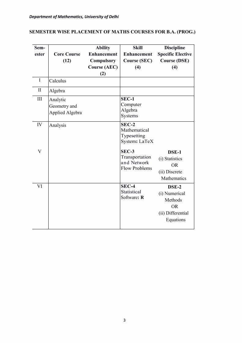
SEMESTER WISE PLACEME�T OF MATHS COURSES FOR B.A. (PROG.)

Sem-

ester

Core Course

(12)

Ability

Enhancement

Compulsory

Course (AEC)

(2)

Skill

Enhancement

Course (SEC)

(4)

Discipline

Specific Elective

Course (DSE)

(4)

I Calculus

II Algebra

III Analytic

Geometry and

Applied Algebra

SEC-1

IV Analysis

V SEC-3

DSE-1

(i) Statistics

OR

(ii) Discrete

Mathematics

VI

DSE-2

(i) Numerical

Methods

OR

(ii) Differential

Equations


4

Semester-I

Paper I: Calculus

Total Marks: 100 (Theory: 75 and Internal Assessment: 25)

Workload: 5 Lectures, 1 Tutorial (per week) Credits: 6 (5+1)

Duration: 14 Weeks (70 Hrs.) Examination: 3 Hours.

Course Objectives: Calculus is referred as 'Mathematics of change' and is concerned with

describing the precise way in which changes in one variable relate to the changes in another.

Through this course, students can understand the quantitative change in the behaviour of the

variables and apply them on the problems related to the environment.

Course Learning Outcomes: The students who take this course will be able to:

i) Understand continuity and differentiability in terms of limits.

ii) Describe asymptotic behavior in terms of limits involving infinity.

iii) Use derivatives to explore the behavior of a given function, locating and classifying

its extrema, and graphing the function.

iv) Understand the importance of mean value theorems.

v) Learn about Maclaurin’s series expansion of elementary functions.

Unit 1: Continuity and Differentiability of Functions

Limits and Continuity, Types of discontinuities; Differentiability of functions, Successive

differentiation, Leibnitz theorem; Partial differentiation, Euler’s theorem on homogeneous

functions.

Unit 2: Tracing of Curves

Tangents and normals, Curvature, Singular points, Asymptotes, Tracing of curves.

Unit 3: Mean Value Theorems and its Applications Rolle’s theorem, Mean value theorems, Applications of mean value theorems to monotonic

functions and inequalities; Taylor’s theorem with Lagrange’s and Cauchy’s forms of remainder,

Taylor’s series, Maclaurin’s series expansion of �� , sin � , cos � , log( 1 + �) and (1 + �)�; Maxima and minima; Indeterminate forms.

References: 1. Anton, Howard, Bivens, Irl, & Davis, Stephen (2013). Calculus (10th ed.). Wiley India

Pvt. Ltd. New Delhi. International Student Version. Indian Reprint 2016.

2. Prasad, Gorakh (2016). Differential Calculus (19th ed.). Pothishala Pvt. Ltd. Allahabad.

Additional Reading:

i. Thomas Jr., George B., Weir, Maurice D., & Hass, Joel (2014). Thomas’ Calculus (13th

ed.). Pearson Education, Delhi. Indian Reprint 2017.

Teaching Plan (Paper-I: Calculus): Weeks 1 and 2: Limits and continuity, Types of discontinuities.

[1] Chapter 1 (Sections 1.1 to 1.6)

[2] Chapter 2 (Section 2.7).

Week 3: Differentiability of functions.


Week 4: Successive differentiation, Leibnitz theorem. [2] Chapter 5.


5

Week 5: Partial differentiation, Euler’s theorem on homogeneous functions.

[2] Sections 12.1 to 12.3.

Week 6: Tangents and normals.

[2] Chapter 8 (Sections 8.1 to 8.3).

Week 7: Curvature, Singular points.

[2] Chapter 10 (Sections 10.1 to 10.3, up to Page 224), and Chapter 11 (Sections 11.1 to 11.4).

Weeks 8 and 9: Asymptotes, Tracing of Curves.

[2] Chapter 9 (Sections 9.1 to 9.6), and Chapter 11 (Section 11.5).

Weeks 10 and 11: Rolle’s theorem, Mean value theorems: Lagrange’s mean value theorem, Cauchy’s

mean value theorem with geometrical interpretations, Applications of mean value theorems to monotonic

functions and inequalities.


Week 12: Taylor’s theorem with Lagrange’s and Cauchy’s forms of remainder, Taylor’s series.


Week 13: Maclaurin’s series expansion of �� , sin � , cos � , log( 1 + �), and (1 + �)�.


Week 14: Maxima and minima; Indeterminate forms.



Facilitating the Achievement of Course Learning Outcomes

Unit

�o. Course Learning Outcomes Teaching and

Learning Activity

Assessment Tasks

1. Understand continuity and differentiability

in terms of limits.

(i) Each topic to be

explained with

illustrations.

(ii) Students to be

encouraged to

discover the

relevant concepts.

(iii) Students to be

given homework/

assignments.

(iv) Discuss and solve

the problems in the

class.

• Presentations and class discussions.

• Assignments and class tests.

• Student presentations.

• Mid-term

examinations.

• End-term examinations.

2. Describe asymptotic behavior in terms of

limits involving infinity.

Use derivatives to explore the behavior of a

given function, locating and classifying its

extrema, and graphing the function.

3. Understand the importance of mean value

theorems. Learn about Maclaurin’s series

expansion of elementary functions.

Keywords: Curvature, Euler’s theorem on homogeneous functions, Leibnitz theorem,

Maclaurin's theorem, Mean value theorems, Indeterminate forms Singular points and asymptotes,

Tangents and normals, Taylor’s series.


6

Semester-II

Paper II: Algebra




Course Objectives: Students will get conceptual understanding and the applicability of the

subject matter. helps students to see how linear algebra can be applied to real-life

situations. Modern concepts and notation are used to introduce the various aspects of linear

equations, leading readers easily to numerical computations and applications.

Course Learning Outcomes: The course will enable the students to understand:

i) Solving higher order algebraic equations.

ii) Become aware of De Moivre’s theorem and its applications.

iii) Solving simultaneous linear equations with at most four unknowns.

iv) Get an overview of abstract algebra by learning about algebraic structures namely,

groups, rings and vector spaces.

Unit 1: Theory of Equations and Expansions of Trigonometric Functions

Fundamental Theorem of Algebra, Relation between roots and coefficients of nth degree

equation, Remainder and factor theorem, Solutions of cubic and biquadratic equations, when

some conditions on roots of the equation are given, Symmetric functions of the roots for cubic

and biquadratic; De Moivre’s theorem (both integral and rational index), Solutions of equations

using trigonometry and De Moivre’s theorem, Expansion for cos ��, sin �� in terms of powers

of cos � , sin �, and cos� � , sin� �, in terms of cosine and sine of multiples of x.

Unit 2: Matrices

Matrices, Types of matrices, Rank of a matrix, Invariance of rank under elementary

transformations, Reduction to normal form, Solutions of linear homogeneous and non-

homogeneous equations with number of equations and unknowns up to four; Cayley−Hamilton

theorem, Characteristic roots and vectors.

Unit 3: Groups, Rings and Vector Spaces

Integers modulo n, Permutations, Groups, Subgroups, Lagrange's theorem, Euler's theorem,

Symmetry Groups of a segment of a line, and regular n-gons for n = 3, 4, 5, and 6; Rings and

subrings in the context of C[0,1] and ℤ�; Definition and examples of a vector space, Subspace and its properties, Linear independence, Basis and dimension of a vector space.

References: 1. Beachy, J. A., & Blair, W. D. (2006). Abstract Algebra (3rd ed.). Waveland Press, Inc.

2. Burnside, William Snow (1979). The Theory of Equations, Vol. 1 (11th ed.) S. Chand &

Co. Delhi. Fourth Indian Reprint.

3. Gilbert, William J., & Vanstone, Scott A. (1993). Classical Algebra (3rd ed.). Waterloo

Mathematics Foundation, Canada.

4. Meyer, Carl D. (2000). Matrix Analysis and Applied Linear Algebra. Society for

Industrial and Applied Mathematics (Siam).

Additional Readings:

i. Dickson, Leonard Eugene (2009). First Course in The Theory of Equations. The Project


7

Gutenberg EBook (http://www.gutenberg.org/ebooks/29785).

ii. Gilbert, William J. (2004). Modern Algebra with Applications (2nd ed.). Wiley-

Interscience, John Wiley & Sons.

Teaching Plan (Paper-II: Algebra):

Weeks 1 and 2: Fundamental Theorem of Algebra (statement only), Relation between roots and

coefficients of nth degree equation, Remainder and Factor Theorem, Solutions of cubic and biquadratic

equations, when some conditions on roots of the equation are given.

[2] Chapter 3.

Week 3: Symmetric functions of the roots for cubic and biquadratic equations.

[2] Chapter 4.

Weeks 4 and 5: De Moivre’s theorem (both integral and rational index), Solutions of equations using

trigonometry and De Moivre’s theorem, Expansion for cos ��, sin �� in terms of powers of cos � , sin �,

and cos� � , sin� �, in terms of cosine and sine of multiples of x. [3] Sections 7.6, and 7.7.

Week 6: Matrices, Types of matrices, Introduction elementary transformations.

[4] Chapter 3 (Sections 3.2, 3.5, and 3.7)

Week 7: Rank of a matrix. Invariance of rank under elementary transformations.

[4] Section 3.9.

Week 8: Reduction to normal (Echelon) form, Solutions of linear homogeneous and non-homogeneous

equations with number of equations and unknowns up to four.


Week 9: Cayley−Hamilton theorem, Characteristic roots and vectors.

[4] Chapter 7 (Section 7.1, and Example 7.2.2)

Week 10: Integers modulo n, Permutations.

[1] Chapter 1 (Section 1.4), and Chapter 2 (Section 2.3).

Week 11: Groups, subgroups, Examples of groups, subgroups and simple theorems.

[1] Chapter 3 (Sections 3.1, and 3.2)

Week 12: Lagrange’s theorem, Euler's theorem, Symmetry groups of a segment of a line, and regular

n-gons for n = 3, 4, 5 and 6; Rings and subrings in the context of C[0,1] and ℤ� .

[1] Chapter 3 (Sections 3.2, 3.3, and 3.6), and Chapter 5 (Section 5.1)

Weeks 13 and 14: Definition and examples of vector space, Subspace and its properties, Linear

independence, Basis and dimension of a vector pace.

[4] Chapter 4 (Sections 4.1, 4.3, and 4.4).


Unit

�o.

Course Learning Outcomes Teaching and Learning

Activity

Assessment Tasks

1. Solving higher order algebraic

equations.

Become aware of De Moivre’s

theorem and its applications.

(i) Each topic to be

explained with examples.

(ii) Students to be involved

in discussions and

encouraged to ask

questions.

(iii) Students to be given

homework/assignments.

(iv) Students to be

encouraged to give short

presentations.


• Participation in discussions.


• Mid-term

examinations.


2. Solving simultaneous linear equations

with at most four unknowns.

3. Get an overview of abstract algebra by

learning about algebraic structures

namely, groups, rings and vector

spaces.

Keywords: Basis and dimension of vector space, Cayley−Hamilton theorem, Characteristic roots

and vectors, Fundamental theorem of algebra, Linear dependence and independence, Lagrange’s

theorem, Permutations, Rank of a matrix.


8

Semester-III

Paper III: Analytic Geometry and Applied Algebra




Course Objectives: The course aims at identifying curves and applying mathematical models in

daily life problems, studying geometric properties of various conic sections. The purpose of this

course is to strengthen the mathematical skills along with the algebraic skills and concepts to

assure success in the algebra.

Course Learning Outcomes: The course will enable the students to:

i) Learn concepts in two-dimensional geometry.

ii) Identify and sketch conics namely, ellipse, parabola and hyperbola.

iii) Learn about three-dimensional objects such as spheres, conicoids, straight lines and

planes using vectors.

iv) Understand various applications of algebra in design of experiments, modelling of

matching jobs, checking spellings, network reliability and scheduling of meetings.

Unit 1: Geometry

Techniques for sketching parabola, ellipse and hyperbola, Reflection properties of parabola,

ellipse, hyperbola and their applications to signals, Classification of quadratic equations

representing lines, parabola, ellipse and hyperbola.

Unit 2: 3-Dimensional Geometry and Vectors

Rectangular coordinates in 3-dimensional space, Spheres, Cylindrical surfaces, Cones, Vectors

viewed geometrically, Vectors in coordinate systems, Vectors determined by length and angle,

Dot product, Cross product and their geometrical properties, Parametric equations of lines in

plane, Planes in 3-dimensional space.

Unit 3: Applied Algebra

Latin squares, Table for a finite group as a Latin square, Latin squares as in design of

experiments, Mathematical models for matching jobs, Spelling checker, Network reliability,

Street surveillance, Scheduling meetings, Interval graph modelling and influence model, Pitcher

pouring puzzle.

References:

1. Anton, Howard; Bivens, Irl & Davis, Stephen (2013). Calculus (10th ed.). Wiley India

Pvt. Ltd. New Delhi. International Student Version. India. Reprint 2016.

2. Gulberg, Jan. (1997). Mathematics from the Birth of !umbers. W.W. Norton & Co.

3. Tucker, Alan (2012). Applied Combinatorics (6th ed.). John Wiley & Sons, Inc.

Additional Reading:

i. Lidl, Rudolf & Pilz, Günter (1998). Applied Abstract Algebra (2nd ed.). Springer. Indian

Reprint 2014.

Teaching Plan (Paper III: Analytic Geometry and Applied Algebra): Weeks 1 to 3: Techniques for sketching parabola, ellipse and hyperbola with problem solving.



9

Weeks 4 and 5: Reflection properties of parabola, ellipse and hyperbola, Classification of quadratic

equation representing lines, parabola, ellipse and hyperbola, Rotation of axis second degree equations

[1] Chapter 11 (Sections 11.4, and 11.5).

Weeks 6 and 7: Rectangular coordinates in 3-dimensional space with problems, Spheres, Cylindrical

surfaces, Cones.


Weeks 8 and 9: Vectors in coordinate systems, Vectors viewed geometrically, Vectors determined by

length and angle, Dot product, Cross product and their geometrical properties.


Weeks 10 and 11: Parametric equations of lines in plane, Planes in 3-dimensional space.

[1] Chapter 12 (Sections 12.4, 12.5).

Weeks 12 to 14: Latin squares, Table for a finite group as a Latin square, Latin squares as in design of

experiments, Mathematical models for matching jobs, Spelling checker, Network reliability, Street

surveillance, Scheduling meetings. Interval graph modelling and Influence model, Pitcher pouring puzzle.

[2] Chapter 5 (Page 195).

[3] Chapter 1 (Section 1.1, Examples 1 to 6), and Chapter 3 (Section 3.2, Example 3, Page 106).


Unit

�o.


Activity

Assessment Tasks

1. Learn concepts in two-dimensional

geometry.

Identify and sketch conics namely,

ellipse, parabola and hyperbola.

(i) Each topic to be explained

with examples.


in discussions and

encouraged to ask

questions.



(iv) Students to be


presentations.




• Mid-term

examinations.


2. Learn about three-dimensional objects

such as spheres, conicoids, straight

lines and planes using vectors.

3. Understand various applications of

algebra in design of experiments,

modelling of matching jobs, checking

spellings, network reliability and

scheduling of meetings.

Keywords: Latin squares, Parabola, Ellipse, Hyperbola, Pitcher pouring puzzle, Spelling

checker.


10

Skill Enhancement Paper

SEC-1: Computer Algebra Systems

Total Marks: 100 (Theory: 38, Internal Assessment: 12, and Practical: 50)

Workload: 2 Lectures, 4 Practicals (per week) Credits: 4 (2+2)

Duration: 14 Weeks (28 Hrs. Theory + 56 Hrs. Practical) Examination: 2 Hrs.

Course Objectives: This course aims at providing basic knowledge to Computer Algebra

Systems (CAS) and their programming language in order to apply them for plotting functions,

finding roots to polynomials, computing limits and other mathematical tools.

Course Learning Outcomes: This course will enable the students to:

i) Use CAS as a calculator and for plotting functions.

ii) Understand the role of CAS finding roots of polynomials and solving general equations.

iii) Employ CAS for computing limits, derivatives, and computing definite and indefinite

integrals.

iv) Use CAS to understand matrix operations and to find eigenvalues of matrices.

Unit 1: Introduction to CAS and Graphics Computer Algebra Systems (CAS), Use of a CAS as a calculator, Simple programming in a

CAS; Computing and plotting functions in 2D, Customizing plots, Animating plots; Producing

table of values, Working with piecewise defined functions, Combining graphics.

Unit 2: Applications in Algebra

Factoring, Expanding and finding roots of polynomials, Working with rational and trigonometric

functions, Solving general equations.

Unit 3: Applications of Calculus

Computing limits, First and higher order derivatives, Maxima and minima, Integration,

Computing definite and indefinite integrals.

Unit 4: Working with Matrices

Performing Gaussian elimination, Operations (transpose, determinant, and inverse), Minors and

cofactors, Solving systems of linear equations, Rank and nullity of a matrix, Eigenvalue,

eigenvector and diagonalization.

References: 1. Bindner, Donald & Erickson, Martin. (2011). A Student’s Guide to the Study, Practice,

and Tools of Modern Mathematics. CRC Press, Taylor & Francis Group, LLC.

2. Torrence, Bruce F., & Torrence, Eve A. (2009). The Student’s Introduction to

Mathematica®: A Handbook for Precalculus, Calculus, and Linear Algebra (2nd ed.).

Cambridge University Press.

�ote: Theoretical and Practical demonstration should be carried out only in one of the CAS:

Mathematica/MATLAB/Maple/Maxima/Scilab or any other.

Practicals to be done in the Computer Lab using CAS Software: [1] Chapter 12 (Exercises 1 to 4 and 8 to 12).

[2] Chapter 3 [Exercises 3.2 (1), 3.3 (1, 2 and 4), 3.4 (1 and 2), 3.5 (1 to 4), 3.6 (2 and 3)].

[2] Chapter 4 (Exercises 4.1, 4.2, 4.5, 4.7 and 4.9).


11

[2] Chapter 5 [Exercises 5.1 (1), 5.3, 5.5, 5.6 (1, 2 and 4), 5.10 (1 and 3), 5.11 (1 and 2)].

[2] Chapter 7 [Exercises 7.1 (1), 7.2, 7.3 (2), 7.4 (1) and 7.6].

Teaching Plan (Theory of SEC-1: Computer Algebra Systems): Weeks 1 and 2: Computer Algebra Systems (CAS), Use of a CAS as a calculator, Simple programming

in a CAS.


Weeks 3 to 5: Computing and plotting functions in 2D, Customizing plots, Animating plots, Producing

table of values, Working with piecewise defined functions, Combining graphics.

[2] Chapter 1, Chapter 3 (Sections 3.1 to 3.6, and 3.8)

Weeks 6 to 8: Factoring, Expanding and finding roots of polynomials, Working with rational and

trigonometric functions, Solving general equations.

[2] Sections 4.1 to 4.3, 4.5 to 4.7, and 4.9.

Weeks 9 to 11: Computing limits, First and higher order derivatives, Maxima and minima, Integration,

computing definite and indefinite integrals.

[2] Chapter 5 (Sections 5.1, 5.3, 5.5, 5.6, 5.10, and 5.11).

Weeks 12 to 14: Performing Gaussian elimination, Operations (transpose, determinant, and inverse),

Minors and cofactors, Solving systems of linear equations, Rank and nullity of a matrix, Eigenvalue,

eigenvector and diagonalization.

[2] Chapter 7 (Sections 7.1 to 7.4, and 7.6 to 7.8).


Unit

�o.


Activity

Assessment Tasks

1. Use CAS as a calculator and for

plotting functions.


with illustrations and

using CAS.

(ii) Students to be given



encouraged to look for

new applications.



• Mid-term

examinations.

• Practical examinations.


2. Understand the role of CAS finding

roots of polynomials and solving

general equations.

3. Employ CAS for computing limits,

derivatives, and computing definite

and indefinite integrals.

4. Use CAS to understand matrix

operations and to find eigenvalues of

matrices.

Keywords: Computer Algebra Systems (CAS), CAS in graphics, CAS in algebra, CAS in

calculus.


12

Semester-IV

Paper IV: Analysis




Course Objectives: The course aims at building an understanding of convergence of sequence

and series of real numbers and various methods/tools to test their convergence. The course also

aims at building understanding of the theory of Riemann integration.


i) Understand basic properties of the field of real numbers.

ii) Examine continuity and uniform continuity of functions using sequential criterion.

iii) Test convergence of sequence and series of real numbers.

iv) Distinguish between the notion of integral as anti-derivative and Riemann integral.

Unit 1: Real numbers and Real Valued Functions

Algebraic and order properties of ℝ, Absolute value and the real line, Suprema and infima, The

completeness and Archimedean property of ℝ; Limit of functions, Sequential criterion for limits, Algebra of limits, Continuous functions, Sequential criterion for continuity and

discontinuity, Properties of continuous functions, Uniform continuity.

Unit 2: Sequence and Series

Sequences and their limits, Convergent sequences, Limit theorems, Monotone sequences and

their convergence, Subsequences, Cauchy sequence and convergence criterion; Infinite series

and their convergence, Cauchy criterion for series, Positive term series, Comparison tests, Absolute and conditional convergence, Cauchy’s nth root test, D’Alembert’s ratio test, Raabe’s test,

Alternating series, Leibnitz test.

Unit 3: Riemann Integral

Riemann integral, Integrability of continuous and monotonic functions.

References:

1. Bartle, Robert G., & Sherbert, Donald R. (2015). Introduction to Real Analysis (4th ed.).

Wiley India Edition.

2. Ross, Kenneth A. (2013). Elementary Analysis: The Theory of Calculus (2nd ed.).

Undergraduate Texts in Mathematics, Springer. Indian Reprint.


i. Bilodeau, Gerald G., Thie, Paul R., & Keough, G. E. (2010). An Introduction to Analysis

(2nd ed.). Jones & Bartlett India Pvt. Ltd. Student Edition. Reprinted 2015.

ii. Denlinger, Charles G. (2011). Elements of Real Analysis. Jones & Bartlett India Pvt. Ltd.

Student Edition. Reprinted 2015.

Teaching Plan (Paper IV: Analysis): Week 1: Algebraic and order properties of ℝ, Absolute value and the real line.

[1] Chapter 2 (Sections 2.1 and 2.2)

Weeks 2 and 3: Suprema and infima, The completeness properties of ℝ, Archimedean property of ℝ. [1] Chapter 2 (Sections 2.3 and 2.4).


13

Weeks 4 and 5: Sequences and their limits, Convergent sequences, Limit theorems.

[1] Chapter 3 (Sections 3.1 and 3.2).

Week 6: Monotone sequences and monotone convergence theorem.


Week 7: Subsequences, Cauchy sequence and Cauchy convergence criterion.

[1] Chapter 3 (Sections 3.4 [3.4.1, 3.4.2, 3.4.3, 3.4.5, 3.4.6{(a), (b)}, 3.4.8 (Statement only) and

3.5 [up to 3.5.6]).

Weeks 8 and 9: Infinite series, Convergence of a series, nth term test, Cauchy’s criterion for series, The

p-series, Positive term series, Comparison tests, Absolute and conditional convergence.

[1] Chapter 3 (Section 3.7), Chapter 9 [Section 9.1 (9.1.1 and 9.1.2)].

Week 10: Cauchy’s nth root test, D’Alembert’s ratio test, Raabe’s test, Alternating series, Leibnitz test.

[1] Chapter 9 [Sections 9.2 (Statements of tests only) and 9.3 (9.3.1 and 9.3.2)].

Week 11: Limit of functions, Sequential criterion for limits, Algebra of limits.


Week 12: Continuous functions, Sequential criterion for continuity and discontinuity, Boundedness

theorem, Intermediate value theorem, Uniform continuity.

[1] Chapter 5 (Sections 5.1, 5.3, and 5.4 excluding continuous extension and approximation)

Week 13: Riemann integral: Upper and lower integrals, Riemann integrable functions.

[2] Chapter 6 (Section 32, only statement of the results up to Page 274, with Examples 1, and 2)

Week 14: Riemann integrability of continuous and monotone functions.

[2] Chapter 6 [Section 33 (33.1 and 33.2)].


Unit

�o.


Activity

Assessment Tasks

1. Understand basic properties of

the field of real numbers.

Examine continuity and

uniform continuity of

functions using sequential

criterion.


with examples.

(ii) Students to be involved in

discussions and encouraged

to ask questions.



(iv) Students to be encouraged

to give short presentations.




• Mid-term

examinations.


2. Test convergence of sequence

and series of real numbers.

3. Distinguish between the notion

of integral as anti-derivative

and Riemann integral.

Keywords: Continuity, Cauchy convergence criterion, Convergence, Cauchy’s nth root test,

D’Alembert’s ratio test, Intermediate value theorem, Riemann integral, Supremum, Uniform

continuity.


14


SEC-2: Mathematical Typesetting System: LaTeX




Course Objectives: The purpose of this course is to help you begin using LaTeX, a

mathematical typesetting system designed for the creation of beautiful books − and especially for

books that contain a lot of mathematics, complicated symbols and formatting.


i) Create and typeset a LaTeX document.

ii) Typeset a mathematical document using LaTex.

iii) Learn about pictures and graphics in LaTex.

iv) Create beamer presentations.

Unit 1: Getting Started with LaTeX

Introduction to TeX and LaTeX, Creating and typesetting a simple LaTeX document, Adding

basic information to documents, Environments, Footnotes, Sectioning, Displayed material.

Unit 2: Mathematical Typesetting

Accents and symbols; Mathematical typesetting (elementary and advanced): Subscript/

Superscript, Fractions, Roots, Ellipsis, Mathematical symbols, Arrays, Delimiters, Multiline

formulas, Putting one thing above another, Spacing and changing style in math mode.

Unit 3: Graphics and PSTricks

Pictures and graphics in LaTeX, Simple pictures using PSTricks, Plotting of functions.

Unit 4: Getting Started with Beamer

Beamer, Frames, Setting up beamer document, Enhancing beamer presentation.

References:

1. Bindner, Donald & Erickson, Martin. (2011). A Student’s Guide to the Study, Practice,


2. Lamport, Leslie (1994). LaTeX: A Document Preparation System, User’s Guide and

Reference Manual (2nd ed.). Pearson Education. Indian Reprint.

Additional Reading:

i. Dongen, M. R. C. van (2012). LaTeX and Friends. Springer-Verlag.

Practicals to be done in the Computer Lab using a suitable LaTeX Editor: [1] Chapter 9 (Exercises 4 to 10), Chapter 10 (Exercises 1, 3, 4, and 6 to 9), and Chapter 11

Exercises 1, 3, 4, 5).

Teaching Plan (Theory of SEC-2: Mathematical Typesetting System: LaTeX): Weeks 1 to 3: Introduction to TeX and LaTeX, Creating and typesetting a simple LaTeX document,

adding basic information to documents, Environments, Footnotes, Sectioning, Displayed material.




15

Weeks 4 to 7: Accents and symbols; Mathematical typesetting (elementary and advanced):

Subscript/Superscript, Fractions, Roots, Ellipsis, Mathematical symbols, Arrays, Delimiters, Multiline

formulas, Putting one thing above another, Spacing and changing style in math mode.



Weeks 8 to 11: Pictures and graphics in LaTeX, Simple pictures using PS Tricks, Plotting of functions.

[1] Chapter 9 (Section 9.8), and Chapter 10 (Sections 10.1 to 10.3)


Weeks 12 to 14: Beamer, Frames, Setting up beamer document, Enhancing beamer presentation.



Unit

�o.

Course Learning

Outcomes

Teaching and Learning

Activity

Assessment Tasks

1. Create and typeset a LaTeX

document.

(i) Topics to be explained

using LaTex editor.



(iii) Students to be encouraged

to look for new

applications.



• Mid-term examinations.



2. Typeset a mathematical

document using LaTex.

3. Learn about pictures and

graphics in LaTex.

4. Create beamer

presentations.

Keywords: LaTex, Mathematical typesetting, PSTricks, Beamer.


16

Semester-V


SEC-3: Transportation and �etwork Flow Problems




Course Objectives: This course aims at providing applications of linear programming to solve

real-life problems such as transportation problem, assignment problem, shortest-path problem,

minimum spanning tree problem, maximum flow problem and minimum cost flow problem.


i) Formulate and solve transportation problems.

ii) Learn to solve assignment problems using Hungarian method.

iii) Solve travelling salesman problem.

iv) Learn about network models and various network flow problems.

v) Learn about project planning techniques namely, CPM and PERT.

Unit 1: Transportation Problems

Transportation problem and its mathematical formulation, North West corner method, Least cost

method and Vogel’s approximation method for determination of starting basic feasible solution,

Algorithm for solving transportation problem.

Unit 2: Assignment and Traveling Salesperson Problems Assignment problem and its mathematical formulation, Hungarian method for solving

assignment problem, Traveling salesperson problem.

Unit 3: �etwork Models

Network models, Minimum spanning tree algorithm, Shortest-route problem, Maximum flow

model.

Unit 4: Project Management with CPM/PERT Project network representation, CPM and PERT.

References:

1. Hillier, Frederick S., & Lieberman, Gerald J. (2017). Introduction to Operations

Research (10th ed.). McGraw Hill Education (India) Pvt. Ltd. New Delhi.

2. Taha, Hamdy A. (2007). Operations Research: An Introduction (8th ed.). Pearson

Education India. New Delhi.

Additional Reading:

i. Bazaraa, Mokhtar S., Jarvis, John J., & Sherali, Hanif D. (2010). Linear Programming

and !etwork Flows (4th ed.). John Wiley & Sons.

Practicals to be done in the Computer Lab using a suitable Software: Use TORA/Excel spreadsheet to solve transportation problem, Assignment problem, Traveling

salesperson problem, Shortest-route problem, Minimum spanning tree algorithm, Maximum flow

model, CPM and PERT calculations of exercises from the Chapters 5 and 6 of [2].


17

[1] Case 9.1: Shipping Wood to Market, and Case 9.3: Project Pickings.

Teaching Plan (Theory of SEC-3: Transportation and �etwork Flow Problems): Weeks 1 to 4: Transportation problem and its mathematical formulation, North West corner method, least

cost method and Vogel’s approximation method for determination of starting basic feasible solution.

Algorithm for solving transportation problem.


Weeks 5 to 7: Assignment problem and its mathematical formulation, Hungarian method for solving

assignment problem, traveling salesperson problem.

[2] Sections 5.4, and 9.3.

Weeks 8 to 11: Network models, minimum spanning tree algorithm, shortest-route problem, maximum

flow model.


Weeks 12 to 14: Project network, CPM and PERT.



Unit

�o.


Activity

Assessment Tasks

1. Formulate and solve transportation

problems.

(i) Topics to be explained

with illustrations using

TORA/Excel.




encouraged to look for

new applications.



• Mid-term

examinations.



2. Learn to solve assignment problems

using Hungarian method.

Solve travelling salesman problem.

3. Learn about network models and

various network flow problems.

4. Learn about project planning

techniques namely, CPM and PERT.

Keywords: Transportation problem, Assignment problem, Traveling salesperson problem,

Network flows, CPM, PERT.


18

Mathematics: Discipline Specific Elective (DSE) Course -1 Any one of the following:

DSE-1 (i): Statistics

DSE-1 (ii): Discrete Mathematics

DSE-1 (i): Statistics




Course Objectives: The course aims at building a strong foundation of theory of statistical

distributions as well as understanding some of the most commonly used distributions. The course

also aims to equip the students to analyze, interpret and draw conclusions from the given data.


i) Determine moments and distribution function using moment generating functions.

ii) Learn about various discrete and continuous probability distributions.

iii) Know about correlation and regression for two variables, weak law of large numbers and

central limit theorem.

iv) Test validity of hypothesis, using Chi-square, F and t-tests, respectively in sampling

distributions.

Unit 1: Probability, Random Variables and Distribution Functions

Sample space, Events, Probability Classical, Relative frequency and axiomatic approaches to

probability, Theorems of total and compound probability; Conditional probability, Independent

events, Baye’s Theorem; Random variables (discrete and continuous), Probability distribution,

Expectation of a random variable, Moments, Moment generating functions.

Unit 2: Discrete and Continuous Probability Distributions

Discrete and continuous distribution, Binomial, Poisson, Geometric, Normal and exponential

distributions, Bivariate distribution, Conditional distribution and marginal distribution,

Covariance, Correlation and regression for two variables, Weak law of large numbers and central

limit theorem for independent and identically distributed random variables.

Unit 3: Sampling Distributions Statistical inference: Definitions of random sample, Parameter and statistic, Sampling

distribution of mean, Standard error of sample mean; Mean, variance of random sample from a

normal population; Mean, variance of random sample from a finite population; Chi-square

distribution, F distribution and t distribution, Test of hypotheses based on a single sample.

References:

1. Devore, Jay L., & Berk, Kenneth N. (2007). Modern Mathematical Statistics with

Applications. Thomson Brooks/Cole.

2. Miller, Irvin & Miller, Marylees (2006). John E. Freund’s: Mathematical Statistics with

Applications (7th ed.). Pearson Education, Asia.


19


i. Hayter, Anthony (2012). Probability and Statistics for the Engineers and Scientists (4th

ed.). Brooks/Cole, Cengage Learning.

ii. Mood, Alexander M., Graybill, Franklin A., & Boes, Duane C. (1974). Introduction to

the Theory of Statistics (3rd ed.). McGraw-Hill Inc. Indian Reprint 2017. iii. Rohtagi, Vijay K., & Saleh, A. K. Md. E. (2001). An Introduction to Probability and

Statistics (2nd ed.). John Wiley & Sons, Inc. Wiley India Edition 2009.

Teaching Plan (DSE-1 (i): Statistics): Week 1: Sample space, Events, Probability Classical, Relative frequency and axiomatic approaches to

probability, Theorems of total and compound probability. [1] Chapter 2 (Sections 2.1 to 2.3).

Week 2: Conditional probability, Independent events, Baye’s theorem.


Week 3: Random Variables, Discrete and continuous random variables, Probability distribution functions

discrete random variables, p.m.f, c.d.f, Expectation, Moments, Moment generating functions of discrete

random variables.


Week 4: Probability Distribution functions continuous random variables, p.d.f, c.d.f, Expectation,

Moments, Moment generating functions of continuous random variables.


Week 5: Discrete distribution: Binomial distribution and its m.g.f., Discrete distribution: Poisson and its

m.g.f.


Week 6: Geometric distribution, Continuous distribution: Normal and its m.g.f.

[1] Chapter 3 (Sections 3.2, and 3.6, excluding negative binomial distribution)

[1] Chapter 4 (Section 6.5)

Weeks 7 and 8: Exponential distribution and its “memoryless” property, Bivariate distribution,

conditional distribution and marginal distribution, Covariance, Correlation and regression.

[1] Chapter 4 (Section 4.3 Pages 193 to 196), and Chapter 5 (Sections 5.1 Exclude more than two

variables, 5.2, and 5.3 omit bivariate normal distribution)

Week 9: Weak law of large numbers and central limit theorem for independent and identically distributed

random variables.


Weeks 10 and 11: Definitions of random sample, Parameter and statistic, Sampling distribution of mean,

Standard error of sample mean, Mean, variance of random sample from a normal population, Mean,

variance of random sample from a finite population.


Week 12: Chi-square distribution, t- distribution and F- distribution.


Weeks 13 and 14: Test of hypotheses based on a single sample.



Unit

�o.


Activity

Assessment Tasks

1. Determine moments and

distribution function using

moment generating functions.


with examples.


in discussions and

encouraged to ask

questions.





• Mid-term

2. Learn about various discrete and

continuous probability

distributions.

Know about correlation and


20

regression for two variables,

weak law of large numbers and

central limit theorem.


(iv) Students to be


presentations.

examinations.


3. Test validity of hypothesis, using

Chi-square, F and t-tests,

respectively in sampling

distributions.

Keywords: Bayes theorem, Binomial, Poisson, Geometric, Normal and exponential

distributions, Central limit theorem, Chi-square distribution, F-distribution and t-distribution,

Correlation and regression for two variables, Moments and moment generating functions, Weak

law of large numbers.


21

DSE-1 (ii): Discrete Mathematics




Course Objectives: Discrete mathematics is the study of mathematical structures that are

fundamentally discrete rather than continuous. The mathematics of modern computer science is

built almost entirely on discrete math, in particular Boolean algebra and graph theory. The aim of

this course is to make the students aware of the fundamentals of lattices, Boolean algebra and

graph theory.

Course Learning Outcomes: The course will enable the students to understand:

i) Learn about partial ordering of sets and various types of lattices.

ii) Learn about Boolean algebra and switching circuits with Karnaugh maps.

iii) Know about basics of graph theory and four color map problem.

Unit 1: Partial Ordering

Definition, Examples and properties of posets, Maps between posets, Algebraic lattice, Lattice as

a poset, Duality principle, Sublattice, Hasse diagrams; Products and homomorphisms of lattices,

Distributive lattice, Complemented lattice.

Unit 2: Boolean Algebra and Switching Circuits

Boolean algebra, Boolean polynomial, CN form, DN form; Simplification of Boolean

polynomials, Karnaugh diagram; Switching circuits and its applications, Finding CN form and

DN form.

Unit 3: Graph Theory

Graphs, Subgraph, Complete graph, Bipartite graph, Degree sequence, Euler’s theorem for sum

of degrees of all vertices, Eulerian circuit, Seven bridge problem, Hamiltonian cycle, Adjacency

matrix, Dijkstra’s shortest path algorithm (improved version), Digraphs; Definitions and

examples of tree and spanning tree, Kruskal’s algorithm to find the minimum spanning tree;

Planar graphs, Coloring of a graph and chromatic number.

Reference: 1. Rosen, Kenneth H. (2011). Discrete Mathematics and its Applications with

Combinatorics and Graph Theory (7th ed.). McGraw-Hill Education Private Limited.

Special Indian Edition.


i. Goodaire, Edgar G. & Parmenter, Michael M. (2011). Discrete Mathematics with Graph

Theory (3rd ed.). Pearson Education (Singapore) Pvt. Ltd. Indian Reprint.

ii. Hunter, David J. (2017). Essentials of Discrete Mathematics (3rd ed.). Jones & Bartlett

Learning, LLC.

iii. Lidl, Rudolf & Pilz, Günter (1998). Applied Abstract Algebra (2nd ed.). Springer. Indian

Reprint 2014.

Teaching plan (DSE-1 (ii): Discrete Mathematics): Week 1: Definition, Examples and properties of posets, Maps between posets.

[1] Chapter 7 (Sections 7.5, and 7.6, Pages 493 to 511)

Weeks 2 and 3: Algebraic lattice, Lattice as a poset, Duality principle, Sublattice, Hasse diagrams;

Products and homomorphisms of lattices, Distributive lattice, Complemented lattice.


22

[1] Chapter 7 (Section 7.6, Pages 511 to 521)

Week 4: Boolean algebra, Boolean polynomial, CN form, DN form.


Week 5: Simplification of Boolean polynomials, Karnaugh diagram.


Week 6: Switching circuits and its applications, Finding CN form and DN form.


Week 7: Graphs, Subgraph, Complete graph, Bipartite graph,


Week 8: Degree sequence, Euler’s theorem for sum of degrees of all vertices.


Week 9: Eulerian circuit, Seven bridge problem, Hamiltonian cycle.


Week 10: Adjacency matrix, Dijkstra’s shortest path algorithm (improved version), Digraphs.


Week 11 and 12: Definitions and examples of tree and spanning tree.

[1] Chapter 9 [Sections 9.1 (Pages 623 to 634), 9.3, and 9.4 (Pages 649 to 673)]

Week 13: Kruskal’s algorithm to find the minimum spanning tree.


Week 14: Planar graphs, coloring of a graph and chromatic number.

[1] Chapter 8 (Section 8.7, and 8.8, Pages 595 to 613).


Unit

�o.

Course Learning

Outcomes

Teaching and Learning Activity Assessment Tasks

1. Learn about partial ordering

of sets and various types of

lattices.

(i) Each topic to be explained with

examples.


discussions and encouraged to

ask questions.



(iv) Students to be encouraged to

give short presentations.




• Mid-term

examinations.


2. Learn about Boolean algebra

and switching circuits with

Karnaugh maps.

3. Know about basics of graph

theory and four color map

problem.

Keywords: CN and DN form, Digraphs and planar graphs, Distributive and complemented

lattice, Eulerian circuit, Karnaugh diagram, Posets and its lattices, Seven bridge problem,

Switching circuits and its applications.


23

Semester-VI


SEC-4: Statistical Software: R




Course Objectives: The purpose of this course is to help you begin using R, a powerful free

software program for doing statistical computing and graphics. It can be used for exploring and

plotting data, as well as performing statistical tests.


i) Be familiar with R syntax and use R as a calculator.

ii) Understand the concepts of objects, vectors and data types.

iii) Know about summary commands and summary table in R.

iv) Visualize distribution of data in R and learn about normality test.

v) Plot various graphs and charts using R.

Unit 1: Getting Started with R - The Statistical Programming Language

Introducing R, using R as a calculator; Explore data and relationships in R; Reading and getting

data into R: combine and scan commands, viewing named objects and removing objects from R,

Types and structures of data items with their properties, Working with history commands,

Saving work in R; Manipulating vectors, Data frames, Matrices and lists; Viewing objects within

objects, Constructing data objects and their conversions.

Unit 2: Descriptive Statistics and Tabulation Summary commands: Summary statistics for vectors, Data frames, Matrices and lists; Summary

tables.

Unit 3: Distribution of Data

Stem and leaf plot, Histograms, Density function and its plotting, The Shapiro−Wilk test for

normality, The Kolmogorov−Smirnov test.

Unit 4: Graphical Analysis with R

Plotting in R: Box-whisker plots, Scatter plots, Pairs plots, Line charts, Pie charts, Cleveland dot

charts, Bar charts; Copy and save graphics to other applications.

References: 1. Bindner, Donald & Erickson, Martin. (2011). A Student’s Guide to the Study, Practice,


2. Gardener, M. (2012). Beginning R: The Statistical Programming Language, Wiley

Publications.

Additional Reading:

i. Verzani, John (2014). Using R for Introductory Statistics (2nd ed.). CRC Press, Taylor &

Francis Group.


24

Practicals to be done in the Computer Lab using Statistical Software R: [1] Chapter 14 (Exercises 1 to 3). [2] Relevant exercises of Chapters 2 to 5, and 7.

�ote: The practical may be done on the database to be downloaded from https://data.gov.in/

Teaching Plan (Theory of SEC-4: Statistical Software: R): Weeks 1 to 3: Introducing R, using R as a calculator; Explore data and relationships in R, Reading and

getting data into R: Combine and scan commands, viewing named objects and removing objects from R,

Types and structures of data items with their properties, Working with history commands, Saving

work in R.


[2] Chapter 2.

Weeks 4 and 5: Manipulating vectors, Data frames, Matrices and lists; Viewing objects within objects,

Constructing data objects and their conversions.

[2] Chapter 3.

Weeks 6 to 8: Summary commands: Summary statistics for vectors, Data frames, Matrices and lists;

Summary tables.

[2] Chapter 4.

Weeks 9 to 11: Stem and leaf plot, Histograms, Density function and its plotting, The Shapiro−Wilk test

for normality, The Kolmogorov-Smirnov test.

[2] Chapter 5.

Weeks 12 to 14: Plotting in R: Box-whisker plots, Scatter plots, Pairs plots, Line charts, Pie charts,

Cleveland dot charts, Bar charts; Copy and save graphics to other applications.


[2] Chapter 7.


Unit

�o.


Activity

Assessment Tasks

1. Be familiar with R syntax and

use R as a calculator.

Understand the concepts of

objects, vectors and data types.

(i) Topics to be explained with illustrations using R

software.



(iii) Students to be encouraged

to look for new

applications.

• Presentations and participation in

discussions.


• Mid-term

examinations.



2. Know about summary

commands and summary table

in R.

3. Visualize distribution of data in

R and learn about normality

test.

4. Plot various graphs and charts

using R.

Keywords: Objects, Vectors, Data types, Summary commands, Shapiro−Wilk test, Bar charts.


25

Mathematics: DSE–2

Any one of the following:

DSE-2 (i): �umerical Methods

DSE-2 (ii): Differential Equations

DSE-2 (i): �umerical Methods




Course Objectives: The goal of this paper is to acquaint students for the study of certain

algorithms that uses numerical approximation for the problems of solving polynomial equations,

transcendental equations, linear system of equations, interpolation, and problems of ordinary

differential equations.

Course Learning Outcomes: After completion of this course, students will be able to:

i) Find the consequences of finite precision and the inherent limits of numerical methods.

ii) Appropriate numerical methods to solve algebraic and transcendental equations.

iii) Solve first order initial value problems of ordinary differential equations numerically

using Euler methods.

Unit 1: Errors and Roots of Transcendental and Polynomial Equations

Floating point representation and computer arithmetic, Significant digits; Errors: Roundoff error,

Local truncation error, Global truncation error, Order of a method, Convergence and terminal

conditions; Bisection method, Secant method, Regula−Falsi method, Newton−Raphson method.

Unit 2: Algebraic Linear Systems and Interpolation

Gaussian elimination method (with row pivoting), Gauss−Jordan method; Iterative methods:

Jacobi method, Gauss−Seidel method; Interpolation: Lagrange form, Newton form, Finite

difference operators, Gregory−Newton forward and backward difference interpolations,

Piecewise polynomial interpolation (Linear and quadratic).

Unit 3: �umerical Differentiation, Integration and ODE

Numerical differentiation: First and second order derivatives, Richardson extrapolation method;

numerical integration: Trapezoidal rule, Simpson’s rule; Ordinary differential equation: Euler’s

method, Modified Euler’s methods (Heun’s and midpoint).

References:

1. Chapra, Steven C. (2018). Applied !umerical Methods with MATLAB for Engineers and

Scientists (4th ed.). McGraw-Hill Education.

2. Fausett, Laurene V. (2009). Applied !umerical Analysis Using MATLAB. Pearson.

India.

3. Jain, M. K., Iyengar, S. R. K., & Jain R. K. (2012). !umerical Methods for Scientific and

Engineering Computation (6th ed.). New Age International Publishers. Delhi.

Additional Reading:

i. Bradie, Brian (2006). A Friendly Introduction to !umerical Analysis. Pearson Education

India. Dorling Kindersley (India) Pvt. Ltd. Third Impression, 2011.


26

Teaching Plan (DSE-2(i): �umerical Methods): Weeks 1 and 2: Floating point representation and computer arithmetic, Significant digits; Errors:

Roundoff error, Local truncation error, Global truncation error; Order of a method, Convergence and

terminal conditions.

[2] Chapter 1 (Sections 1.2.3, 1.3.1, and 1.3.2).

[3] Chapter 1 (Sections 1.2, 1.3).

Week 3 and 4: Bisection method, Secant method, Regula−Falsi method, Newton−Raphson method.



Week 5: Gaussian elimination method (with row pivoting), Gauss−Jordan method; Iterative methods:

Jacobi method, Gauss−Seidel method.

[2] Chapter 3 (Sections 3.1, and 3.2), Chapter 6 (Sections 6.1, and 6.2)


Week 6: Interpolation: Lagrange form, and Newton form.


[3] Chapter 4 (Section 4.2)

Weeks 7 and 8: Finite difference operators, Gregory−Newton forward and backward difference

interpolations.


Week 9: Piecewise polynomial interpolation: Linear and quadratic.

[2] Chapter 8 [Section 8.3 (8.3.1, and 8.3.2)].


Weeks 10, 11 and 12: Numerical differentiation: First and second order derivatives, Richardson

extrapolation method; Numerical integration: Trapezoidal rule, Simpson’s rule.

[2] Chapter 11 [Sections 11.1 (11.1.1, 11.1.2 and 11.1.4), and 11.2 (11.2.1, and 11.2.2)]

Weeks 13 and 14: Ordinary differential equations: Euler’s method, Modified Euler’s methods (Heun’s

and midpoint).

[1] Chapter 22 (Sections 22.1, 22.2 (up to Page 583) and 22.3).


Unit

�o.


Activity

Assessment Tasks

1. Find the consequences of finite

precision and the inherent limits

of numerical methods.

(i) Each topic to be explained with examples.


discussions and encouraged

to ask questions.



(iv) Students to be encouraged

to give short presentations.


discussions.


• Mid-term

examinations.


2. Appropriate numerical methods

to solve algebraic and

transcendental equations.

3. Solve first order initial value

problems of ordinary differential

equations numerically using

Euler methods.

Keywords: Bisection method, Euler’s method, Gauss−Jordan method, Gauss−Seidel method,

Jacobi method, Newton−Raphson method, Regula−Falsi method, Richardson extrapolation

method, Secant method and Simpson’s rule.


27

DSE-2 (ii): Differential Equations




Course objectives: The course aims at introducing ordinary and partial differential equations to

the students and finding their solutions using various techniques with the tools needed to model complex real-world situations.

Course learning outcomes: The course will enable the students to:

i) Solve ODE’s and know about Wronskian and its properties.

ii) Method of variation of parameters and total differential equations.

iii) Solve linear PDE’s of first order.

iv) Understand Lagrange’s and Charpit’s methods for solving nonlinear PDE’s of first order.

Unit1: Ordinary Differential Equations

First order exact differential equations including rules for finding integrating factors, First order

higher degree equations solvable for x, y, p and Clairut’s equations; Wronskian and its

properties, Linear homogeneous equations with constant coefficients; The method of variation of

parameters; Euler’s equations; Simultaneous differential equations; Total differential equations.

Unit 2: Linear Partial Differential Equations

Order and degree of partial differential equations, Concept of linear partial differential equations,

Formation of first order partial differential equations, Linear partial differential equations of first

order and their solutions.

Unit 3: �on-linear Partial Differential Equations

Concept of non-linear partial differential equations, Lagrange’s method, Charpit’s method,

classification of second order partial differential equations into elliptic, parabolic and hyperbolic

through illustrations only.

References:

1. Ross, Shepley L. (1984). Differential Equations (3rd ed.). John Wiley & Sons, Inc.

2. Sneddon, I. N. (2006). Elements of Partial Differential Equations, Dover Publications.

Indian Reprint.

Additional Readings: i. Anton, Howard, Bivens, Irl, & Davis, Stephen (2013). Calculus (10th ed.). John Wiley &

Sons Singapore Pvt. Ltd. Reprint (2016) by Wiley India Pvt. Ltd. Delhi.

ii. Brannan, James R., Boyce, William E., & McKibben, Mark A. (2015). Differential

Equations: An Introduction to Modern Methods and Applications (3rd ed.). John Wiley &

Sons, Inc.

Teaching Plan (DSE-2 (ii): Differential Equations): Weeks 1 and 2: First order exact differential equations including rules for finding integrating factors.


Weeks 3 and 4: First order higher degree equations solvable for x, y, p and Clairut’s equations.


Weeks 5 and 6: Wronskian and its properties, Linear homogeneous equations with constant coefficients.


Week 7: The method of variation of parameters, Euler’s equations.


28


Week 8: Simultaneous differential equations, Total differential equations.

[2] Chapter 1 (Sections 2, 3, 5, and 6)

Week 9: Order and degree of partial differential equations, Concept of linear partial differential

equations, Formation of first order partial differential equations.


Weeks 10 and 11: Statement of Theorem 2 with applications, Linear partial differential equations of first

order and their solutions.

[2] Chapter 2 (Sections 3, 4, 5, and 6).

Week 12: Statements of Theorems 4, 5, and 6 with applications, Concept of non-linear partial differential

equations, Lagrange’s method.

[2] Chapter 2 (Sections 7, 8, and 9).

Weeks 13 and 14: Charpit’s method, Classification of second order partial differential equations into

elliptic, Parabolic and hyperbolic through illustrations only.

[2] Chapter 2 (Section 10), and Chapter 3 (Sections 1, and 5).


Unit

�o.

Course Learning Outcomes Teaching and Learning Activity Assessment Tasks

1. Solve ODE’s and know about

Wronskian and its properties.

Method of variation of

parameters and total

differential equations.

(i) Each topic to be explained with examples.


discussions and encouraged to

ask questions.



(iv) Students to be encouraged to

give short presentations.


discussions.


• Mid-term

examinations.


2. Solve linear PDE’s of first

order.

3. Understand Lagrange’s and

Charpit’s methods for solving

nonlinear PDE’s of first order.

Keywords: Charpit's method, Clairut’s equations, Euler’s equations, Lagrange’s method,

Wronskian and its properties.


29

Acknowledgments

The following members were actively involved in drafting the LOCF syllabus of

B.A. (Programme), University of Delhi.

Head

• C.S. Lalitha, Department of Mathematics

Coordinator

• Hemant Kumar Singh, Department of Mathematics

Committee Members

• Sarla Bhardwaj (Dr. Bhim Rao Ambedkar College)

• Anuradha Gupta (Delhi College of Arts and Commerce)

• A.R. Prasannan (Maharaja Agrasen College)

uiversity of delhi departmet of mathematics b.a. …du.ac.in/du/uploads/revisedsyllabi1/annexure-76....

Documents