ucge reports - university of calgary | home · ucge reports number 20206 department of geomatics...
TRANSCRIPT

UCGE Reports Number 20206
Department of Geomatics Engineering The Influence of Target Acceleration on Dual-Channel
SAR-GMTI (Synthetic Aperture Radar Ground Moving Target Indication) Data
(URL: http://www.geomatics.ucalgary.ca/links/GradTheses.html)
by
Jayanti Sharma
October 2004

THE UNIVERSITY OF CALGARY
The influence of target acceleration on dual-channel SAR-GMTI (synthetic aperture
radar ground moving target indication) data
by
Jayanti Sharma
A THESIS
SUBMITTED TO THE FACULTY OF GRADUATE STUDIES
IN PARTIAL FULFILLMENT OF THE REQUIREMENTS FOR THE
DEGREE OF MASTER OF SCIENCE
DEPARTMENT OF GEOMATICS ENGINEERING
CALGARY, ALBERTA
OCTOBER, 2004
c© Jayanti Sharma 2004

Abstract
This thesis investigates the effects of acceleration on the detection and estimation
of the velocity of ground moving targets in airborne dual-channel synthetic aperture
radar (SAR) data. The airborne results give an indication of the performance we
may expect in an upcoming spaceborne system, the GMTI (ground moving target
indication) mode of RADARSAT-2.
Acceleration has (i) an insignificant impact on the detection of moving targets
using the displaced phase centre antenna (DPCA) algorithm; (ii) only minor affects
on the estimation of across-track velocity (the component perpendicular to the line of
flight) using along-track interferometric (ATI) phase and (iii) may significantly bias
the estimate of along-track velocity. Estimation of both acceleration and velocity
components is not uniquely determined using only two receive channels.
Acceleration also has severe effects on focusing. Time-frequency analysis is used to
improve target focusing and to detect the presence of significant target acceleration.
ii

Acknowledgements
I would like to thank Dr. Chuck Livingstone and my supervisor Dr. Michael Collins
for providing me the unique opportunity of combining work experience at a defence
research facility with a Master’s degree. Chuck has done an amazing job directing the
GMTI group and focusing our collective energy towards the RADARSAT-2 launch
date. I thank Dr. Collins for allowing me considerable flexibility in conducting my
research, and for providing long distance supervision from Calgary to Ottawa.
I would like to especially thank Dr. Christoph Gierull for his invaluable guidance
and advice at all stages of the research, and Mr. Ishuwa Sikaneta for his help and depth
of knowledge of mathematics, radar, linux, and LATEX. I am grateful to the entire
GMTI team at DRDC Ottawa including Shen Chiu, Sean Gong, Marielle Quinton
and Pete Beaulne for their help and patience, and for providing an enjoyable and
stimulating environment in which to work. Finally I thank my parents for their
support, encouragement, and for fostering in me a love of learning.
This work has been financed by Defence Research and Development Canada -
Ottawa, and I have been supported by the National Science and Engineering Research
Council, the University of Calgary, and Alberta Learning. Their financial support is
greatly appreciated.
iii

Table of Contents
Abstract ii
Acknowledgements iii
Table of Contents iv
List of Tables vi
List of Tables vii
List of Figures vii
List of Figures viii
List of Symbols xiii
List of Abbreviations xvi
1 Introduction 11.1 Background . . . . . . . . . . . . . . . . . . . . . . . . . . . . . . . . 11.2 Research objectives . . . . . . . . . . . . . . . . . . . . . . . . . . . . 51.3 Thesis organization . . . . . . . . . . . . . . . . . . . . . . . . . . . . 5
2 SAR-GMTI background and theory 82.1 SAR fundamentals . . . . . . . . . . . . . . . . . . . . . . . . . . . . 82.2 Classic MTI . . . . . . . . . . . . . . . . . . . . . . . . . . . . . . . . 132.3 Multi-aperture GMTI . . . . . . . . . . . . . . . . . . . . . . . . . . . 15
2.3.1 Range compressed signal . . . . . . . . . . . . . . . . . . . . . 162.3.2 Multi-aperture GMTI techniques . . . . . . . . . . . . . . . . 24
2.4 Time-frequency analysis . . . . . . . . . . . . . . . . . . . . . . . . . 302.4.1 Introduction . . . . . . . . . . . . . . . . . . . . . . . . . . . . 302.4.2 Utility of TF analysis . . . . . . . . . . . . . . . . . . . . . . . 312.4.3 Time-frequency transformations . . . . . . . . . . . . . . . . . 33
3 Detection 403.1 Theory . . . . . . . . . . . . . . . . . . . . . . . . . . . . . . . . . . . 40
3.1.1 DPCA mathematical representation . . . . . . . . . . . . . . . 413.1.2 Analysis of the DPCA expression . . . . . . . . . . . . . . . . 43
iv

3.2 Simulations . . . . . . . . . . . . . . . . . . . . . . . . . . . . . . . . 443.2.1 DPCA magnitude with vy0 . . . . . . . . . . . . . . . . . . . . 453.2.2 DPCA magnitude with vx0 . . . . . . . . . . . . . . . . . . . . 473.2.3 DPCA magnitude with ay0 . . . . . . . . . . . . . . . . . . . . 493.2.4 DPCA magnitude with along-track acceleration ax0 . . . . . . 513.2.5 DPCA magnitude with ay0 . . . . . . . . . . . . . . . . . . . . 533.2.6 DPCA magnitude for spaceborne geometries . . . . . . . . . . 533.2.7 Analysis of DPCA magnitude simulations on target detection 57
3.3 Experimental results . . . . . . . . . . . . . . . . . . . . . . . . . . . 593.3.1 Detection and tracking algorithm . . . . . . . . . . . . . . . . 593.3.2 Analysis and results of experimental detections . . . . . . . . 63
4 Focusing 684.1 Theory and simulations . . . . . . . . . . . . . . . . . . . . . . . . . . 68
4.1.1 Focusing a stationary target . . . . . . . . . . . . . . . . . . . 694.1.2 Focusing a moving target with a SWMF . . . . . . . . . . . . 704.1.3 Focusing a moving target with a matched reference filter . . . 96
4.2 Experimental Results . . . . . . . . . . . . . . . . . . . . . . . . . . . 1024.2.1 Focusing a stationary target . . . . . . . . . . . . . . . . . . . 1034.2.2 Focusing a moving target with a SWMF . . . . . . . . . . . . 1044.2.3 Focusing a moving target with a matched reference filter . . . 107
5 Estimation of along-track velocity vx0 1115.1 Theory and Simulations . . . . . . . . . . . . . . . . . . . . . . . . . 112
5.1.1 Estimating vx0 for a target with only along-track velocity . . . 1125.1.2 Estimating vx0 in the presence of vy0 . . . . . . . . . . . . . . 1145.1.3 Estimating vx0 in the presence of ay0 . . . . . . . . . . . . . . 1185.1.4 Estimating vx0 in the presence of ax0 . . . . . . . . . . . . . . 1205.1.5 Estimating vx0 in the presence of ay0 . . . . . . . . . . . . . . 1245.1.6 Estimating vx0 in a spaceborne geometry . . . . . . . . . . . . 124
5.2 Experimental Results . . . . . . . . . . . . . . . . . . . . . . . . . . . 127
6 Estimation of across-track velocity vy0 1336.1 Theory . . . . . . . . . . . . . . . . . . . . . . . . . . . . . . . . . . . 1336.2 Simulations . . . . . . . . . . . . . . . . . . . . . . . . . . . . . . . . 134
6.2.1 Variation in ATI with vy0 . . . . . . . . . . . . . . . . . . . . 1356.2.2 Variation in ATI with vx0 . . . . . . . . . . . . . . . . . . . . 1386.2.3 Variation in ATI with ay0 . . . . . . . . . . . . . . . . . . . . 1406.2.4 Variation in ATI with ax0 and ay0 . . . . . . . . . . . . . . . . 1436.2.5 Variation in ATI phase for spaceborne scenarios . . . . . . . . 143
v

6.2.6 ATI simulation summary . . . . . . . . . . . . . . . . . . . . . 1446.3 Experimental Results . . . . . . . . . . . . . . . . . . . . . . . . . . . 146
6.3.1 Across-track velocity estimation algorithm . . . . . . . . . . . 1466.3.2 Analysis of estimated velocities . . . . . . . . . . . . . . . . . 148
7 Acceleration detection and focusing improvements 1527.1 Theory . . . . . . . . . . . . . . . . . . . . . . . . . . . . . . . . . . . 153
7.1.1 Tracking the instantaneous frequency . . . . . . . . . . . . . . 1537.1.2 Detecting acceleration using TF analysis . . . . . . . . . . . . 1557.1.3 Focusing using TF Analysis . . . . . . . . . . . . . . . . . . . 157
7.2 Simulations . . . . . . . . . . . . . . . . . . . . . . . . . . . . . . . . 1587.2.1 Tracking the instantaneous frequency . . . . . . . . . . . . . . 1587.2.2 Detecting acceleration using TF analysis . . . . . . . . . . . . 1607.2.3 Focusing using TF Analysis . . . . . . . . . . . . . . . . . . . 173
7.3 Experimental Results . . . . . . . . . . . . . . . . . . . . . . . . . . . 1767.3.1 TF transform . . . . . . . . . . . . . . . . . . . . . . . . . . . 1767.3.2 Tracking the instantaneous frequency . . . . . . . . . . . . . . 1777.3.3 Detecting acceleration using TF analysis . . . . . . . . . . . . 1797.3.4 Focusing using TF Analysis . . . . . . . . . . . . . . . . . . . 182
8 Conclusions and extensions 1868.1 Conclusions . . . . . . . . . . . . . . . . . . . . . . . . . . . . . . . . 1868.2 Extensions . . . . . . . . . . . . . . . . . . . . . . . . . . . . . . . . . 189
References 198
A Experimental data 199A.1 Experimental set up . . . . . . . . . . . . . . . . . . . . . . . . . . . 199A.2 Data pre-processing . . . . . . . . . . . . . . . . . . . . . . . . . . . . 202A.3 Motion parameter estimation accuracies . . . . . . . . . . . . . . . . 204
A.3.1 GPS accuracies . . . . . . . . . . . . . . . . . . . . . . . . . . 207
B ATI ambiguities and performance analysis 211B.1 ATI ambiguities . . . . . . . . . . . . . . . . . . . . . . . . . . . . . . 211
B.1.1 Directional ambiguities . . . . . . . . . . . . . . . . . . . . . . 211B.1.2 Blind-speed ambiguities . . . . . . . . . . . . . . . . . . . . . 213B.1.3 Doppler ambiguities . . . . . . . . . . . . . . . . . . . . . . . 213
B.2 Performance analysis . . . . . . . . . . . . . . . . . . . . . . . . . . . 217B.2.1 Coherence . . . . . . . . . . . . . . . . . . . . . . . . . . . . . 221
vi

List of Tables
3.1 Radar and geometry parameters for airborne SAR simulations. . . . . 453.2 Radar and geometry parameters for RADARSAT-2 simulations. . . . 54
A.1 Radar and geometry parameters for CV 580 Petawawa data collectionin November 2000. . . . . . . . . . . . . . . . . . . . . . . . . . . . . 199
A.2 A comparison of along-track velocities estimated using the filter-bankmethod from dual-channel SAR data and GPS. . . . . . . . . . . . . 205
A.3 A comparison of across-track velocities estimated using along-trackinterferometric phase from dual-channel SAR data and GPS. . . . . . 206
A.4 A comparison of the absolute differences in along- and across-trackvelocities estimated using SAR data and velocities estimated from GPS.207
A.5 Transforming GPS speed and heading into along-track and across-trackvelocities. . . . . . . . . . . . . . . . . . . . . . . . . . . . . . . . . . 208
vii
List of Figures
1.1 Artist’s rendition of the RADARSAT-2 sensor c©CSA. . . . . . . . . . 3
2.1 Doppler frequency of a moving target shifted out of the clutter band-width, enabling its detection. . . . . . . . . . . . . . . . . . . . . . . 14
2.2 Top-down view of antenna and accelerating target geometry for anairborne scenario. . . . . . . . . . . . . . . . . . . . . . . . . . . . . . 17
2.3 Top-down view of antenna and target geometry for two-channel datacollection. . . . . . . . . . . . . . . . . . . . . . . . . . . . . . . . . . 20
2.4 Classical DPCA geometry. . . . . . . . . . . . . . . . . . . . . . . . . 26
3.1 Range compressed DPCA magnitude through time for a simulated tar-get with constant velocity vy0 varied from -25 to 25 m/s and vx0 = 0. 46
3.2 Range compressed DPCA magnitude through time for a simulated tar-get with constant velocity vx0 varied from -25 to 25 m/s and vy0 = 0. 47
3.3 Range compressed DPCA magnitude through time for a simulated tar-get with constant velocity vx0 = −25 m/s and vy0 varied from -25 to25 m/s. . . . . . . . . . . . . . . . . . . . . . . . . . . . . . . . . . . 48
3.4 Range compressed DPCA magnitude through time for a simulated tar-get with constant velocities vx0 = −25 m/s and vy0 = 1 m/s. . . . . . 49
3.5 Range compressed DPCA magnitude through time for a simulated tar-get with constant across-track acceleration ay0 varied from -1 to 1 m/s2. 50
3.6 Range compressed DPCA magnitude through time for a simulated tar-get with constant along-track acceleration ax0 varied from -1 to 1 m/s2. 52
3.7 Range compressed DPCA magnitude through time for a simulated tar-get with time-varying across-track acceleration with rate of change ay0
varied from -0.1 to 0.1 m/s3. . . . . . . . . . . . . . . . . . . . . . . . 533.8 Range compressed DPCA magnitude through time for a simulated tar-
get observed in a spaceborne geometry with across-track velocity vy0
varied from -25 to 25 m/s. . . . . . . . . . . . . . . . . . . . . . . . . 553.9 Range compressed DPCA magnitude through time for a simulated tar-
get observed in a spaceborne geometry with constant across-track ac-celeration ay0 varied from -1 to 1 m/s2. . . . . . . . . . . . . . . . . . 56
3.10 Four stages of the target detection and tracking process operating inthe range compressed domain. . . . . . . . . . . . . . . . . . . . . . . 61
3.11 Variation of target velocity (obtained from GPS) through time in thevicinity of broadside time t=0 for a single pass. . . . . . . . . . . . . 65
3.12 Range compressed DPCA magnitude through time for one pass of theJuliet target. . . . . . . . . . . . . . . . . . . . . . . . . . . . . . . . 67
viii

4.1 Magnitude response (after azimuth compression) of simulated non-accelerating point targets focused using a SWMF versus azimuthaldistance. . . . . . . . . . . . . . . . . . . . . . . . . . . . . . . . . . . 73
4.2 Example TF representation of a SWMF and a target moving in theacross-track direction with vy > 0 m/s. . . . . . . . . . . . . . . . . . 74
4.3 Example TF representation of a SWMF and a target moving in theacross-track direction with sufficient vy > 0 m/s such that the Dopplerfrequency wraps across the ±PRF/2 boundary. . . . . . . . . . . . . 76
4.4 Example TF representation of a SWMF and a target moving in theacross-track direction with vx > 0 m/s. . . . . . . . . . . . . . . . . . 77
4.5 Magnitude response (after azimuth compression) of simulated pointtargets with constant acceleration focused using a SWMF. . . . . . . 79
4.6 Across-track acceleration ay(t) (with constant ay0) and correspondingacross-track velocity vy(t) for a point target through time. The target’sazimuth response is given in Figure 4.7. . . . . . . . . . . . . . . . . . 82
4.7 Magnitude response (after azimuth compression) of a simulated pointtarget (with constant ay0 and an ay(t) given in Figure 4.6) focusedusing a SWMF. . . . . . . . . . . . . . . . . . . . . . . . . . . . . . . 83
4.8 Across-track acceleration ay(t) (a rectangular window centred at broad-side) and corresponding across-track velocity vy(t) for a point targetthrough time whose azimuth response to a SWMF is given in Figure 4.9. 85
4.9 Magnitude response (after azimuth compression) of a simulated pointtarget (with time-varying across-track acceleration given in Figure 4.8)focused using a SWMF. . . . . . . . . . . . . . . . . . . . . . . . . . 86
4.10 Across-track acceleration ay(t) (a rectangular window centred at 1.3 spast broadside) for a simulated point target, corresponding across-trackvelocity vy(t), and its magnitude response (after azimuth compression)when focused using a SWMF. . . . . . . . . . . . . . . . . . . . . . . 88
4.11 Across-track acceleration ay(t) (a unit step function with height 0.1m/s2) and corresponding across-track velocity vy(t) for a point targetthrough time whose azimuth response to a SWMF is given in Figure4.13. . . . . . . . . . . . . . . . . . . . . . . . . . . . . . . . . . . . . 89
4.12 Across-track acceleration ay(t) (which is ramped until broadside) andcorresponding across-track velocity vy(t) for a point target throughtime whose azimuth response to a SWMF is given in Figure 4.13. . . 90
4.13 Magnitude response (after azimuth compression) of simulated pointtargets (with time-varying across-track accelerations given in Figures4.11 and 4.12) focused using a SWMF. . . . . . . . . . . . . . . . . . 91
ix

4.14 Magnitude response (after azimuth compression) of simulated non-accelerating point targets focused using a SWMF for a spacebornegeometry. . . . . . . . . . . . . . . . . . . . . . . . . . . . . . . . . . 93
4.15 Magnitude response (after azimuth compression) of simulated pointtargets with constant acceleration focused using a SWMF for a space-borne geometry. . . . . . . . . . . . . . . . . . . . . . . . . . . . . . . 95
4.16 Impulse responses of simulated point targets focused using perfectlymatched filters. . . . . . . . . . . . . . . . . . . . . . . . . . . . . . . 99
4.17 Magnitude response after azimuth compression of a stationary cornerreflector from the Ottawa 2001 data set. . . . . . . . . . . . . . . . . 105
4.18 Magnitude response (after clutter suppression using DPCA) for a mov-ing target (l1p9 Convoy) focused using a SWMF. . . . . . . . . . . . 106
4.19 DPCA magnitude after azimuth compression of one pass of the Convoytarget using a SWMF and a MTMF. . . . . . . . . . . . . . . . . . . 108
4.20 DPCA magnitude after azimuth compression of one pass of the Juliettarget using a SWMF and a MTMF. . . . . . . . . . . . . . . . . . . 109
5.1 Magnitude responses of a simulated point target with constant vx0 = 10m/s after compression with a bank of reference filters initialized withvarious vx0 velocities. . . . . . . . . . . . . . . . . . . . . . . . . . . . 115
5.2 DPCA magnitude responses of a simulated point target with vy0 = 30m/s after compression with a bank of reference filters initialized withvarious vx0 velocities. . . . . . . . . . . . . . . . . . . . . . . . . . . . 117
5.3 Magnitude responses of a simulated point target with ay0 = 0.1 m/s2
after compression with a bank of reference filters initialized with variousvx0. . . . . . . . . . . . . . . . . . . . . . . . . . . . . . . . . . . . . . 119
5.4 Magnitude responses of a simulated point target with ax0 = 0.5 m/s2
after compression with a bank of reference filters initialized with vary-ing vx0. . . . . . . . . . . . . . . . . . . . . . . . . . . . . . . . . . . . 121
5.5 Example TF history for a target accelerating in the along-track direction.1235.6 Magnitude responses of a simulated point target with ay0 = 0.04 m/s3
after compression with a bank of reference filters initialized with variousvx0 velocities. . . . . . . . . . . . . . . . . . . . . . . . . . . . . . . . 125
5.7 Magnitude responses of a simulated point target for a spaceborne ge-ometry with vx0 = 10 m/s after compression with a bank of referencefilters initialized with various vx0 velocities. . . . . . . . . . . . . . . . 126
5.8 DPCA filter-bank magnitude map from one pass of the Convoy target(line 1, pass 5). . . . . . . . . . . . . . . . . . . . . . . . . . . . . . . 129
5.9 DPCA filter-bank magnitude map from one pass of the Juliet target(line 2, pass 2). . . . . . . . . . . . . . . . . . . . . . . . . . . . . . . 130
x

5.10 DPCA filter-bank magnitude map from one pass of the Juliet target(line 3, pass 3). . . . . . . . . . . . . . . . . . . . . . . . . . . . . . . 131
6.1 ATI signal for varying across-track velocities vy0. . . . . . . . . . . . . 1366.2 ATI signal for varying across-track velocities vy0 and constant vx0 =
−30 m/s compared with the expected ATI phase when the vx0 depen-dence is neglected. . . . . . . . . . . . . . . . . . . . . . . . . . . . . 139
6.3 Compressed target response from a SWMF and ATI signal for a pointtarget with vx0 = 10 m/s. . . . . . . . . . . . . . . . . . . . . . . . . 141
6.4 ATI signal for varying across-track broadside velocities vy0 and con-stant across-track acceleration ay0 = 1 m/s2 compared with the ex-pected ATI phase when the ay0 dependence is neglected. . . . . . . . 142
6.5 ATI signal (with normalized magnitude) for various experimental tar-get tracks. . . . . . . . . . . . . . . . . . . . . . . . . . . . . . . . . . 150
7.1 Instantaneous frequency of a simulated target with constant velocity(vx0 = 10 m/s, vy0 = 15 m/s, SCR = 0 dB) tracked through azimuthalslow-time. . . . . . . . . . . . . . . . . . . . . . . . . . . . . . . . . . 158
7.2 Enlarged portion of Figure 7.1. . . . . . . . . . . . . . . . . . . . . . 1597.3 Instantaneous frequency of a simulated target in a spaceborne geometry
with slow constant velocity (vy0 = 3 m/s and SCR = 0 dB) trackedthrough azimuthal slow-time. . . . . . . . . . . . . . . . . . . . . . . 161
7.4 Absolute error in the mean value of the cubic coefficient (of a poly-nomial fit to the DPCA phase) for a simulated target moving withconstant velocity as a function of SCR. . . . . . . . . . . . . . . . . . 166
7.5 Inverse variance of the cubic coefficient (of a polynomial fit to theDPCA phase) for a simulated target moving with constant velocity asa function of SCR. . . . . . . . . . . . . . . . . . . . . . . . . . . . . 167
7.6 Absolute error in the mean value of the cubic coefficient (of a polyno-mial fit to the DPCA phase) for a simulated accelerating target as afunction of SCR. . . . . . . . . . . . . . . . . . . . . . . . . . . . . . 168
7.7 Inverse variance of the cubic coefficient (of a polynomial fit to theDPCA phase) for a simulated accelerating target as a function of SCR. 169
7.8 Unwrapped DPCA phase through azimuthal slow-time for a targetwith an SCR of 0 dB moving with constant velocity. . . . . . . . . . . 171
7.9 Normalized DPCA magnitude of a simulated accelerating target fo-cused using instantaneous phase from IF integration. . . . . . . . . . 174
7.10 Normalized DPCA magnitude of a simulated accelerating target fo-cused using conventional SAR processing. . . . . . . . . . . . . . . . . 175
7.11 DPCA magnitude of a target track (l1p9 Convoy) in the TF domainafter application of the PWVD. . . . . . . . . . . . . . . . . . . . . . 177
xi

7.12 Instantaneous frequency of a vehicle target (l1p9 Convoy) through az-imuth time. . . . . . . . . . . . . . . . . . . . . . . . . . . . . . . . . 178
7.13 Antenna gain pattern of the receiving fore antenna for the CV 580system. . . . . . . . . . . . . . . . . . . . . . . . . . . . . . . . . . . . 180
7.14 Differences between a target’s TF track f(t) and its linear, quadratic,and cubic fits over time. . . . . . . . . . . . . . . . . . . . . . . . . . 181
7.15 DPCA magnitudes of a vehicle target (l1p9 Convoy) focused usingmatched filters derived from various TF histories. . . . . . . . . . . . 183
7.16 DPCA magnitude of a vehicle target (l1p9 Convoy) focused using areference filter initialized with vx0 and vy0 computed from a matchedfilter-bank and from the ATI phase, respectively. . . . . . . . . . . . . 185
A.1 Delta control target from the Petawawa 2000 data collection. . . . . . 201A.2 Sketch of Juliet and Delta moving target rail systems with their sur-
rounding structure and environment. . . . . . . . . . . . . . . . . . . 201A.3 Four vehicle convoy from the Petawawa 2000 data collection. . . . . . 202A.4 Aerial photograph mosaic of CFB Petawawa training area, site of the
2000 GMTI experiment. . . . . . . . . . . . . . . . . . . . . . . . . . 203
B.1 Example TF representation of a SWMF and a target moving in theacross-track direction with sufficient vy0 > 0 m/s such that there iszero spectral overlap between the target and reference signals. . . . . 216
B.2 Illustration of the across-track interferometric (ATI) signal in the com-plex plane for a moving target with accompanying clutter. . . . . . . 220
xii

List of Symbols
A : signal amplitude . . . . . . . . . . . . . . . . . . . . . . . . . . . . . . . . . . . . . . . . . . . . . . . . . 10
ax0 : target along-track acceleration at broadside time t = 0 . . . . . . . . . . 18
ay0 : target across-track acceleration at broadside time t = 0 . . . . . . . . . 18
Bν : pulse bandwidth . . . . . . . . . . . . . . . . . . . . . . . . . . . . . . . . . . . . . . . . . . . . . . . . 10
c : speed of light . . . . . . . . . . . . . . . . . . . . . . . . . . . . . . . . . . . . . . . . . . . . . . . . . . . . . 10
d : physical antenna separation distance . . . . . . . . . . . . . . . . . . . . . . . . . . . . . . 19
fnyq : Nyquist frequency . . . . . . . . . . . . . . . . . . . . . . . . . . . . . . . . . . . . . . . . . . . . 213
fPRF : pulse repetition frequency . . . . . . . . . . . . . . . . . . . . . . . . . . . . . . . . . . . . . 18
fsta lims : frequency limits of stationary world reference filter . . . . . . . . . 215
g(t) : difference in the two-way path length to the fore and registered aftapertures . . . . . . . . . . . . . . . . . . . . . . . . . . . . . . . . . . . . . . . . . . . . . . . . . . . . . . . . . . . . .23
H : altitude of radar platform . . . . . . . . . . . . . . . . . . . . . . . . . . . . . . . . . . . . . . . .18
I(t) : azimuth compressed target image . . . . . . . . . . . . . . . . . . . . . . . . . . . . . . 68
j : imaginary unit . . . . . . . . . . . . . . . . . . . . . . . . . . . . . . . . . . . . . . . . . . . . . . . . . . . . . 9
k = 2πλ
: wave number . . . . . . . . . . . . . . . . . . . . . . . . . . . . . . . . . . . . . . . . . . . . . . . .21
λ : wavelength . . . . . . . . . . . . . . . . . . . . . . . . . . . . . . . . . . . . . . . . . . . . . . . . . . . . . . . 10
ν0 : carrier frequency . . . . . . . . . . . . . . . . . . . . . . . . . . . . . . . . . . . . . . . . . . . . . . . . . . 9
ρ : correlation coefficient (coherence) . . . . . . . . . . . . . . . . . . . . . . . . . . . . . . . . 159
r(t) : reference signal for matched filtering . . . . . . . . . . . . . . . . . . . . . . . . . . . 69
<{·} : retains the real component of the argument . . . . . . . . . . . . . . . . . . . 37
xiii
R0 : range to target at broadside time t = 0 . . . . . . . . . . . . . . . . . . . . . . . . . . 18
R(t) : range to the target as a function of time . . . . . . . . . . . . . . . . . . . . . . . 18
R1(t) : range from fore antenna to the target as a function of time . . . 19
R2(t) : range from aft antenna to the target as a function of time . . . . 19
Rn(0) : nth derivative of range function evaluated at t = 0 . . . . . . . . . . . 18
rect(x/L) : Rectangular function of length L . . . . . . . . . . . . . . . . . . . . . . . . . 11
sinc(x) = sin(x)x
: . . . . . . . . . . . . . . . . . . . . . . . . . . . . . . . . . . . . . . . . . . . . . . . . . . . . 11
σx : standard deviation of x . . . . . . . . . . . . . . . . . . . . . . . . . . . . . . . . . . . . . . . . .210
S(ω) = F{s(t)} =∫∞−∞ s(t)e−jωtdt : Fourier transform . . . . . . . . . . . . . . . . 10
s(t) : range compressed target signal . . . . . . . . . . . . . . . . . . . . . . . . . . . . . . . . . 12
t : time variable (azimuthal or slow-time) . . . . . . . . . . . . . . . . . . . . . . . . . . . . 11
timg : azimuthal time at which azimuth compressed target signalis focused . . . . . . . . . . . . . . . . . . . . . . . . . . . . . . . . . . . . . . . . . . . . . . . . . . . . . . . . . . . . 80
t0 : azimuthal broadside time t = 0 . . . . . . . . . . . . . . . . . . . . . . . . . . . . . . . . . 178
τ : time variable (for one pulse or fast-time) . . . . . . . . . . . . . . . . . . . . . . . . . . . 9
T : synthetic aperture time . . . . . . . . . . . . . . . . . . . . . . . . . . . . . . . . . . . . . . . . . . 12
θ(t) : phase history function . . . . . . . . . . . . . . . . . . . . . . . . . . . . . . . . . . . . . . . . . 27
~v : vector . . . . . . . . . . . . . . . . . . . . . . . . . . . . . . . . . . . . . . . . . . . . . . . . . . . . . . . . . . . . 24
~vT : transpose . . . . . . . . . . . . . . . . . . . . . . . . . . . . . . . . . . . . . . . . . . . . . . . . . . . . . . . 23
~v∗ : complex conjugation . . . . . . . . . . . . . . . . . . . . . . . . . . . . . . . . . . . . . . . . . . . . . 27
va : aircraft velocity . . . . . . . . . . . . . . . . . . . . . . . . . . . . . . . . . . . . . . . . . . . . . . . . . .16
xiv

vx0 : target along-track velocity at broadside time t = 0 . . . . . . . . . . . . . . 18
vy0 : target across-track velocity at broadside time t = 0 . . . . . . . . . . . . . .18
y0 : target across-track position at broadside time t = 0 . . . . . . . . . . . . . . 18
〈x〉 : expectation . . . . . . . . . . . . . . . . . . . . . . . . . . . . . . . . . . . . . . . . . . . . . . . . . . . .219
|x| : absolute value . . . . . . . . . . . . . . . . . . . . . . . . . . . . . . . . . . . . . . . . . . . . . . . . . . .11
x : mean value . . . . . . . . . . . . . . . . . . . . . . . . . . . . . . . . . . . . . . . . . . . . . . . . . . . . . . . 60
x = dx(t)dt
: first-order time derivative . . . . . . . . . . . . . . . . . . . . . . . . . . . . . . . . . 18
x = d2x(t)dt2
: second-order time derivative . . . . . . . . . . . . . . . . . . . . . . . . . . . . . 184
xv

List of Abbreviations
A/D: Analog to Digital conversion . . . . . . . . . . . . . . . . . . . . . . . . . . . . . . . . . . . .10
ATI: Along-Track Interferometry . . . . . . . . . . . . . . . . . . . . . . . . . . . . . . . . . . . . . . 5
CFAR: Constant False Alarm Rate . . . . . . . . . . . . . . . . . . . . . . . . . . . . . . . . . . . 42
CNR: Clutter-to-Noise Ratio . . . . . . . . . . . . . . . . . . . . . . . . . . . . . . . . . . . . . . . . 219
CRLB: Cramer-Rao Lower Bound . . . . . . . . . . . . . . . . . . . . . . . . . . . . . . . . . . . 163
CV: Convair . . . . . . . . . . . . . . . . . . . . . . . . . . . . . . . . . . . . . . . . . . . . . . . . . . . . . . . . . . .2
DPCA: Displaced Phase Centre Antenna . . . . . . . . . . . . . . . . . . . . . . . . . . . . . . 5
FFT: Fast Fourier Transform . . . . . . . . . . . . . . . . . . . . . . . . . . . . . . . . . . . . . . . . . 30
GMTI: Ground Moving Target Indication . . . . . . . . . . . . . . . . . . . . . . . . . . . . . 1
GPS: Global Positioning System . . . . . . . . . . . . . . . . . . . . . . . . . . . . . . . . . . . . . . . 6
ICM: Internal Clutter Motion . . . . . . . . . . . . . . . . . . . . . . . . . . . . . . . . . . . . . . . . 26
IF: Instantaneous Frequency . . . . . . . . . . . . . . . . . . . . . . . . . . . . . . . . . . . . . . . . 153
LFM: Linear Frequency Modulation . . . . . . . . . . . . . . . . . . . . . . . . . . . . . . . . . . 11
MODEX: Moving Object Detection Experiment . . . . . . . . . . . . . . . . . . . . . . . 2
MTI: Moving Target Indication . . . . . . . . . . . . . . . . . . . . . . . . . . . . . . . . . . . . . . 13
MTMF: Moving Target Matched Filter . . . . . . . . . . . . . . . . . . . . . . . . . . . . . . 107
PRI: Pulse Repetition Interval . . . . . . . . . . . . . . . . . . . . . . . . . . . . . . . . . . . . . . . 24
PRF: Pulse Repetition Frequency . . . . . . . . . . . . . . . . . . . . . . . . . . . . . . . . . . . . 14
PWVD: Pseudo Wigner-Ville Distribution . . . . . . . . . . . . . . . . . . . . . . . . . . . . . 5
xvi

RF: Radio Frequency . . . . . . . . . . . . . . . . . . . . . . . . . . . . . . . . . . . . . . . . . . . . . . . . . . 9
RCS: Radar Cross Section . . . . . . . . . . . . . . . . . . . . . . . . . . . . . . . . . . . . . . . . . . . . . 9
SAR: Synthetic Aperture Radar . . . . . . . . . . . . . . . . . . . . . . . . . . . . . . . . . . . . . . . 1
SCR: Signal-to-Clutter Ratio . . . . . . . . . . . . . . . . . . . . . . . . . . . . . . . . . . . . . . . . . 96
SNR: Signal-to-Noise Ratio . . . . . . . . . . . . . . . . . . . . . . . . . . . . . . . . . . . . . . . . . . .10
STAP: Space Time Adaptive Processing . . . . . . . . . . . . . . . . . . . . . . . . . . . . . . 26
SWMF: Stationary World Matched Filter . . . . . . . . . . . . . . . . . . . . . . . . . . . . 69
TF: Time-Frequency . . . . . . . . . . . . . . . . . . . . . . . . . . . . . . . . . . . . . . . . . . . . . . . . . 30
WVD: Wigner-Ville Distribution . . . . . . . . . . . . . . . . . . . . . . . . . . . . . . . . . . . . . 36
xvii

1
Chapter 1
Introduction
1.1 Background
Synthetic aperture radar (SAR) systems have been used extensively in the past two
decades for fine resolution mapping and other remote sensing applications [72]. Since
the SAR principle for developing high resolution radar images was first suggested
by Carl Wiley in 1954 [63], many airborne and spaceborne SAR systems have been
used operationally. SAR is an active, coherent, all-weather, day-night imaging system
which operates in the microwave region of the electromagnetic spectrum [90]. It has
been used in such diverse applications as land use and topographic mapping, polar
ice research, studies of ocean dynamics, and military surveillance and reconnaissance
[30, 53, 72, 82].
With the advancement of sophisticated SAR signal processing and imaging meth-
ods, more specialized radar problems are being studied including the detection, pa-
rameter estimation, and imaging of ground moving targets in a SAR scene [82]. In
many civilian and military applications of airborne and spaceborne SAR imaging, it
is desirable to simultaneously monitor ground traffic [37, 79].
In the past, detection and tracking of moving targets was primarily a military
concern and was performed by specialized airborne sensors. Extensive investment by
the military resulted in the development of operational airborne platforms (such as
Joint-STARS, developed by the United States in the late 1980’s) which were able to
detect and map vehicles moving on the Earth’s surface [35]. In addition to military
ground moving target indication (GMTI) systems, today there exist several experi-
mental airborne SAR-GMTI radars including Environment Canada’s Convair (CV)

2
580 [49], the German AER-II and PAMIR sensors [25, 28], and a C-band Andover
system developed by the Defence Evaluation Research Agency in the UK [55].
However, with the rapid evolution of radar technology, it is now economically feasi-
ble to also create spaceborne sensors to perform moving target detection and measure-
ment [35]. From a military perspective, such spaceborne systems have the potential to
significantly augment existing operational capabilities by offering increased coverage
and the ability to monitor unfriendly territories. For civilian applications, space-
borne GMTI can provide land and sea traffic monitoring capabilities which may be
valuable in designing, monitoring, and controlling transportation infrastructure [35].
Additional applications of both spaceborne and airborne GMTI have been envisioned
to include intelligence collection, counter-terrorism operations, customs, immigration
and law enforcement, search and rescue, and remote exploration, as well as support
for conventional military roles [23].
Due to the large capital costs associated with the development and operation of
airborne GMTI sensors, these systems are expensive even by military standards, and
have not been used for transportation system monitoring or other civilian applications
to date [35]. Spaceborne sensors, on the other hand, are unmanned, are able to
function 24 hours a day, and support large coverage areas, which increases their
attractiveness for commercial applications.
Presently no spaceborne radar system has GMTI capability, although several SAR
systems with GMTI modes will be launched in the near future [35]. The Canadian
RADARSAT-2 sensor (scheduled for launch in the spring of 2005 [51]) will offer an
experimental moving object detection mode (abbreviated MODEX ), and will provide
the first opportunity to routinely measure and monitor vehicles moving on the Earth’s
surface from space. An artist’s rendition of the RADARSAT-2 sensor is shown in Fig-
ure 1.1. RADARSAT-2 was designed primarily as an imaging radar, thus imposing
limitations on its ability to perform GMTI. However, MODEX will be a valuable
tool in evaluating assumptions made in modelling spaceborne GMTI, developing im-

3
Figure 1.1: Artist’s rendition of the RADARSAT-2 sensor c©CSA [51].
proved processing algorithms for the spaceborne case, identifying the strengths and
weaknesses of single-pass spaceborne SAR-GMTI, and demonstrating potential appli-
cations to interested parties [35]. A second commercial spaceborne SAR with GMTI
capability is the German TerraSAR-X, scheduled for a launch date of spring 2006
[91]; it is hoped that together these sensors will provide further understanding of
spaceborne GMTI.
Despite the numerous applications of SAR-GMTI, there are significant challenges
in detecting and measuring target motion from airborne and spaceborne platforms.
SAR forms high resolution images using phase information in the received echoes. The
instantaneous phase is determined by the relative motion between the radar sensor
and the scene, and the resulting image focusing and quality is dependent (among
other things) upon the ability to reconstruct this phase [20, 89] . SAR imaging
from both spaceborne and airborne radars of stationary scenes is well understood
[83]. However, in the presence of unknown target motion, the target will appear
defocused and spatially displaced from its true location in the image. Numerous
papers (e.g. [17, 20, 35, 41, 67, 80, 90, 93]) have examined the response of a SAR
to moving targets and have suggested methods for estimating the target motion and
achieving a focused image. However, in the majority of GMTI literature, it is assumed

4
that targets travel with constant velocity (e.g. [5, 11, 36, 41, 49, 56, 80, 82]). This
assumption is often violated in real world applications such as monitoring vehicle
traffic on roads and highways, where target acceleration is commonplace and must be
considered.
There has been little published research examining the impacts of target accelera-
tion on GMTI directly. Although some papers include one component of acceleration
in the standard range equations for completeness (e.g. [62, 68]), there are no pa-
pers (to this author’s knowledge) which examine the effects of target acceleration in
experimental data. Yadin [93] notes in passing that target acceleration during the
integration time results in a varying apparent angular position of the target and thus
a smearing in azimuth, although this variation in position is not quantified. Soumekh
[82] observes in the analysis of his experimental data (consisting of military vehicles)
that the focused peaks of some targets seem ‘chaotic’ and ‘not localized’ which he
attributes to target maneuvering and/or target acceleration or deceleration.
Carrara [12] has examined the effects of uncompensated motion of an airborne
platform on focusing. In the preivous paragraphs, it was described how a SAR sig-
nal’s instantaneous phase is determined by the relative radar-target motion. Uncom-
pensated platform motion (possibly due to errors in motion compensation routines)
introduces errors in this phase, which may be equivalent to errors due to uncom-
pensated target motion. Carrara noted that higher-order phase errors from residual
platform motion can cause defocusing effects in the processed imagery.
These observations suggest that acceleration has an impact upon target focusing,
providing the rationale for a more systematic examination of acceleration, and its
potential effects on focusing as well as on the closely-related tasks of detection and
parameter estimation.

5
1.2 Research objectives
The primary objective of this research is to examine the influence of acceleration on
detection, velocity estimation, and focusing of moving targets in dual-channel SAR
data. Theory, simulations, and the analysis of experimental data will be used to
determine acceleration’s effects on detection, and to describe the detrimental effects
of both constant and time-varying accelerations on estimating target motion and on
target focusing if left uncompensated.
The secondary objective is to determine a method of detecting target acceleration
and to compensate for its effects to obtain a focused target image. Although the
acceleration parameters themselves cannot be uniquely determined using only two
channels of SAR data, possibilities lie in detecting certain acceleration components
and obtaining a focused image irrespective of the target motion.
1.3 Thesis organization
Chapter 2 provides the necessary background and theory regarding SAR and GMTI.
The SAR response to a stationary point target is reviewed, followed by an overview of
both classical and multi-aperture GMTI techniques with an emphasis on the displaced
phase centre antenna (DPCA) method and along-track interferometry (ATI). Other
detection and estimation techniques are also reviewed. In addition to analysis of
the SAR time-series signal, further insight may be gained by transforming the data
into a two-dimensional time-frequency space. The utility of time-frequency analysis
is described, and a review of various transformation methods including the Pseudo
Wigner-Ville Distribution (PWVD) is provided.
Chapter 3 examines the impact of acceleration on target detection when using the
DPCA technique. The theoretical DPCA response for a range compressed accelerat-
ing point target is derived, and its repercussions on detection are examined through
simulations of an airborne geometry. The DPCA technique is then used to detect

6
moving targets in experimental data collected using the CV 580 airborne SAR, and
comparisons are made with the theoretical and simulated results.
Chapter 4 describes effects of acceleration on focusing a moving point target in
dual-channel SAR data. The response of a SAR to a stationary target and its response
to moving (possibly accelerating) targets when using conventional azimuth processing
are compared, and the influence of different reference filters on target focusing are
examined. Following the theoretical analysis, stationary and moving targets from
experimental data are compressed in the azimuth dimension using various reference
filters, and their responses are examined in context to the previous results.
Chapters 5 and 6 examine the influence of target acceleration on estimation of
the along-track and across-track target velocity components, respectively. The esti-
mation methods and the effects of acceleration on each velocity component are very
different, which is why they are separated. Each chapter begins with a description
of the estimation algorithm, where along-track velocity estimation makes use of a
bank of matched filters and across-track velocity estimation employs along-track in-
terferometric phase. The effects of each motion component (along- and across-track
velocities and accelerations) on estimation of the velocity vector are examined sepa-
rately using simulations. Lastly, the accuracy in estimating the velocity of targets in
experimental data are determined using comparisons with GPS (Global Positioning
System) data.
Having examined the effects of target acceleration on detection, focusing and pa-
rameter estimation, chapter 7 investigates methods of detecting certain components
of acceleration (specifically along-track acceleration and time-varying across-track ac-
celeration) and focusing a target irrespective of its motion. The suggested algorithms
make use of the instantaneous frequency of the target SAR signal, which is extracted
from the time-frequency domain. An acceleration detection algorithm is proposed
based on polynomial fits to the range and/or frequency history of the target, and a
focusing algorithm is suggested involving reconstruction of the target phase history

7
through integration of the instantaneous frequency. Simulations are used to assess
these algorithms, after which they are applied to experimental data.
A summary of the research and recommendations for future work are presented
in the closing chapter.

8
Chapter 2
SAR-GMTI background and theory
The challenge of SAR-GMTI is to detect moving targets, estimate their motion pa-
rameters, and then focus and insert them into the imaged scene [49]. Generally there
is no a priori knowledge of the targets and we thus start from a stationary-scene
assumption. There exist many different techniques to perform SAR-GMTI, although
all require fundamental understanding of the SAR image formation process.
In this chapter, certain basics of synthetic aperture radar are reviewed, followed
by a brief history of GMTI including classical techniques using a single channel.
Presently, the development of more sophisticated radar systems collecting multi-
channel SAR data has increased the robustness and accuracy of GMTI within var-
ious clutter environments. Experimental airborne systems in use today and future
spaceborne systems are reviewed, and a description of multi-channel techniques and
time-frequency techniques for detection and parameter estimation of moving targets is
provided. The advantages of joint time-frequency analysis over strictly time-domain
methods is investigated, and the properties of various time-frequency transforms are
described.
2.1 SAR fundamentals
The basic purpose of SAR is to derive an image, which is a map of the microwave
reflectivity of a scene [64]. In every monostatic SAR system an antenna transmits a
series of radar pulses, and receives the reflected energy from scatterers. Scatterers may
include moving targets (of primary interest in GMTI) and clutter such as buildings,
fields, and trees, where clutter refers to any unwanted returns that may interfere with
the detection of the desired targets [16]. Time delays between the transmission and

9
reception of each pulse provide information on the range to the targets [90].
SARs are generally coherent, meaning that they retain information regarding both
the amplitude and phase of the received signal [74]. The amplitude is related to the
radar cross section (RCS) of the target, where RCS is a measure of the target’s ability
to reflect electromagnetic waves [16]. The phase is related to the range history of the
target, i.e. the changing distance between the radar platform and the scatterer over
time as the radar sweeps by. To form a SAR image, an accurate model of the imaging
system, the transmitted signal, the imaging geometry, and its evolution through time
is necessary [49]. If any of these are unknown (such as in GMTI), the task of detecting
and focusing a target will be made more complex.
Let the azimuth direction (or along-track) be the dimension parallel to the radar’s
line of flight, and let the range direction (also called across-track) be perpendicular
to the line of flight. When imaging a stationary scene, a SAR achieves fine range
resolution through pulse (or range) compression and high azimuth resolution through
cross-correlating a theoretical stationary target’s phase response with the collected
data (also called azimuth compression) [45]. Imaging stationary targets is a special
case of the general GMTI scenario, and many of processing steps are shared in com-
mon including range compression. The following description of range compression
follows that of [13] and [73].
Assume that the radar transmits a single RF (radio frequency) pulse of the form
n(τ) with complex envelope g(τ) and carrier frequency ν0 :
n(τ) = g(τ) exp(j2πν0τ), (2.1)
where j is the imaginary unit, and τ represents the time scale over one pulse in the
range direction (also known as fast-time). Imagine a scenario in which the radar pulse
reflects off a point target on the ground located at distance R from the radar, and
returns to the antenna. It is assumed that the radar does not move between pulse
transmission and reception (i.e. that R is constant during that time). For typical
airborne and spaceborne SAR systems, this motion can be considered negligible [81].

10
The received signal (from any target, moving or stationary) is analog and must be
digitized, requiring an A/D converter (analog-to-digital) operating at a sampling rate
above the signal bandwidth and with a sufficient number of bits to maintain image
fidelity [63]. In this treatment the signals are presented in their continuous forms to
simplify notation and mathematical manipulation, although in reality all signals will
be sampled and digitized prior to further processing.
The received pulse r(τ) is a delayed and scaled version of the transmitted signal
n(τ),
r(τ) = A(θ, β)g
(τ − 2R
c
)exp
(j2πν0
(τ − 2R
c
)), (2.2)
where c represents the speed of light, and a round-trip time delay of 2R/c has been
introduced. The received signal is multiplied by a positive amplitude factor A, deter-
mined by the target’s reflectivity as well as the elevation angle θ and azimuth angle
β to the target, which in turn dictates the antenna gain applied. Next, the signal
is processed by a typical chain of RF downconversion and intermediate frequency
bandpass filtering in order to strip off the carrier frequency [41] and obtain the target
echo signal e(t):
e(τ) = A(θ, β)g
(τ − 2R
c
)exp
(−j
4πR
λ
), (2.3)
where λ is the carrier wavelength of the signal, related to the carrier frequency by
λ = c/ν0. The shape of pulse envelope g(τ) determines the range resolution of the
radar, where resolution is defined as the ability to separate two scatterers located at
slightly different ranges [73]. Ideally, g(τ) should approach an impulse function, but
practical limits on the bandwidth of the radar will limit the resolution. For improved
signal-to-noise ratios (SNRs) it is desirable to use the radar bandwidth Bν uniformly
such that
|G(ν)| ∝ rect(ν/Bν), (2.4)
where G(ν) is the Fourier transform of g(τ), |G(ν)| is its absolute value, and the

11
rectangular function is defined as:
rect(x) =
1 for |x| ≤ 1/2
0 for |x| > 1/2.
The time-domain function fulfilling the requirement of equation 2.4 is g(τ) = sinc(τBν).
If range resolution is defined as the half-power (-3 dB) width of g(τ), then the reso-
lution in metres ρres is approximately
ρres = 0.886c
2Bν
. (2.5)
However, in order to avoid the practical difficulties in transmitting pulses with a high
peak power, usually longer pulses are generated instead of narrow sinc-functions. The
most common pulse coding is the chirp function with envelope:
g(τ) = exp(jπaτ 2)rect
(τa
Bν
), (2.6)
where a is the frequency rate. The instantaneous phase of the chirp is aπτ 2, and
thus the phase rate of change or frequency is 2aπτ , which is linear in τ , such that
the chirp is also known as a linear frequency modulated (LFM) pulse. The chirp
can be compressed into a sinc-function through cross-correlation with a chirp of the
same frequency rate a, leading to a range resolution given in equation 2.5 [73]. This
cross-correlation operation is also termed matched filtering or range compression.
A single radar LFM pulse after range compression can thus be represented by a
simplified version of equation 2.3:
e(τ) = A(θ, β)sinc(τBν) exp
(−j
4πR
λ
), (2.7)
where the pulse bandwidth Bν is determined by multiplying the frequency rate a (in
units of Hz/s) by the duration of the pulse. A series of such pulses form the signal
received from a point target through azimuthal slow-time (represented by the variable
t). The amplitude of the response will change through t as the sensor advances in the
along-track direction, changing the direction of arrival of the target signal (where this

12
direction is typically represented by the so-called directional cosine u(t)). The range
to the target will also be dependent upon azimuthal slow-time as the radar sweeps
by.
The target energy for each pulse in the range dimension is concentrated along the
peak of the sinc function from equation 2.7. Extracting the target signal along these
peaks for each pulse, and assuming that the target is in the beam of the antenna for
duration T seconds gives the following target signal s(t) after pulse compression:
s(t) = A(u(t)) exp
(−j
4πR(t)
λ
)rect
(t
T
). (2.8)
Following range compression, the signal is corrected for range migration, which
- to a first approximation - consists of a linear term (known as range walk) and a
quadratic term (known as range curvature). Range walk occurs if the antenna beam
centre is oriented off-broadside (i.e. squinted) [63]. Range walk may also occur in
the presence of target motion, although this portion of range walk is not corrected
at this time. Range curvature occurs if the range to a stationary target changes by
more than one range resolution cell over the observation interval, and is of greatest
concern for long-range systems such as spaceborne SARs [63]. Further information
on the correction of range migration is available in [73, 87].
Next the signal is compressed in azimuth to form the SAR image. It is azimuth
compression which separates real aperture radar from synthetic aperture radar. A
real aperture radar has an azimuthal resolution proportional to the beamwidth, and
thus an impractically large antenna is required to create a narrow beam for fine
azimuth resolution [16, 63]. Synthetic aperture radar uses a wide beam to collect the
returns from multiple pulses, and then synthesizes a narrow beam by filtering the
array of pulses after data collection [78]. Moving targets require a slightly different
filter function than stationary targets in order to obtain a properly focused image,
although the matched filtering principle is the same. Further details on all steps of
the SAR image formation process and algorithms for focusing stationary targets are
provided in [9, 13, 29, 73, 87].

13
2.2 Classic MTI
SAR processing was originally developed to image the stationary world [37]. When
conventional processing (as described in section 2.1) is applied to SAR data containing
moving target returns, the targets inevitably appear smeared and defocused in the
image. However, it has been only relatively recently that researchers have combined
both SAR and GMTI capabilities to simultaneously form images of the terrain and
to detect, estimate motion parameters, and focus ground moving targets.
Prior to SAR-GMTI were MTI (moving-target indication) ground systems, which
did not form images, but were used only to detect moving targets. The purpose of
these surface systems was to reject any signals from fixed or slow-moving scatterers
such as buildings, hills, trees, sea and rain, and retain, for detection or display, any
signals from moving targets such as aircraft [76]. Consecutive radar pulses were
compared, and if the reflection times to a scatterer changed between pulses, it was a
potential moving target.
The basic principle behind both MTI and GMTI is to utilize the Doppler shift
imparted on a reflected radar signal in order to distinguish moving targets from fixed
ones [76]. The Doppler shift is related to the velocity of the target in the across-track
(or range) direction. The first airborne MTI systems grew out of airborne early-
warning radars developed by the U.S. Navy to detect low-flying aircraft approaching
forces below. Moving the radars from the ground to an airborne platform greatly
increased the available coverage area, although the high platform altitude, mobility,
and speed, as well as restrictions on size, weight, and power consumption of the
radar presented new challenges to the designers of MTI systems [84]. Additional
complications arose in the airborne scenario (compared to the ground scenario) since
the clutter collected by the radar changes over time, thus hindering the ability to
detect moving targets.
Classical airborne MTI assumes that the Doppler shift of a moving target may be
observable directly in each return signal [62]. While the range bandwidth of a SAR

14
is generally too large to observe the Doppler shift, the azimuthal bandwidth may be
small enough such that the shift due to target motion displaces the signal’s Doppler
outside the clutter bandwidth, and the presence of the target becomes evident (see
Figure 2.1). Whether or not one can detect moving targets using a single-channel MTI
Azimuth (pixel)
Freq
uenc
y (H
z)
0 1000 2000 3000 4000 5000 6000 7000 8000
−300
−200
−100
0
100
200
300
Target signal outside clutter band
Clutter Bandwidth
Figure 2.1: Doppler frequency of a moving target shifted out of the clutter bandwidth,enabling its detection. These data were collected using an airborne platform with apulse repetition frequency of 600 Hz (corresponding to a frequency band of ± 300Hz) and a clutter bandwidth of ± 116 Hz. Courtesy of Shen Chiu, DRDC Ottawa[19].
system depends on the pulse repetition frequency (PRF), the antenna beamwidth
(which in turn determines the clutter spectral width), and the target velocities of
interest.
The basic limitation of single-channel MTI is that the moving target Doppler shift
must be greater than the clutter Doppler spectrum width [62], such that a portion of
the target signal falls outside of the clutter background and may be detected. This is
achieved using a high PRF and a narrow azimuth antenna beamwidth [54]. However,
this method has several shortcomings, including difficulties in detecting targets with
small across-track velocity components (and therefore small Doppler shifts) since the
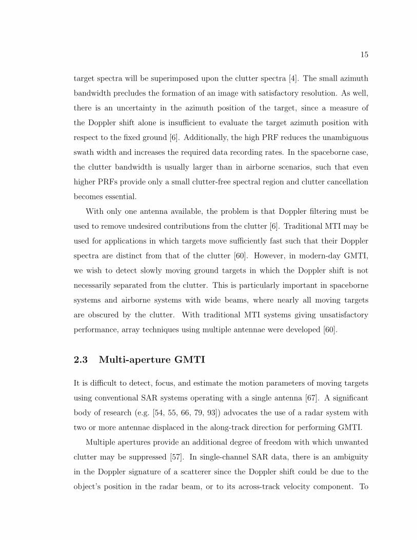
15
target spectra will be superimposed upon the clutter spectra [4]. The small azimuth
bandwidth precludes the formation of an image with satisfactory resolution. As well,
there is an uncertainty in the azimuth position of the target, since a measure of
the Doppler shift alone is insufficient to evaluate the target azimuth position with
respect to the fixed ground [6]. Additionally, the high PRF reduces the unambiguous
swath width and increases the required data recording rates. In the spaceborne case,
the clutter bandwidth is usually larger than in airborne scenarios, such that even
higher PRFs provide only a small clutter-free spectral region and clutter cancellation
becomes essential.
With only one antenna available, the problem is that Doppler filtering must be
used to remove undesired contributions from the clutter [6]. Traditional MTI may be
used for applications in which targets move sufficiently fast such that their Doppler
spectra are distinct from that of the clutter [60]. However, in modern-day GMTI,
we wish to detect slowly moving ground targets in which the Doppler shift is not
necessarily separated from the clutter. This is particularly important in spaceborne
systems and airborne systems with wide beams, where nearly all moving targets
are obscured by the clutter. With traditional MTI systems giving unsatisfactory
performance, array techniques using multiple antennae were developed [60].
2.3 Multi-aperture GMTI
It is difficult to detect, focus, and estimate the motion parameters of moving targets
using conventional SAR systems operating with a single antenna [67]. A significant
body of research (e.g. [54, 55, 66, 79, 93]) advocates the use of a radar system with
two or more antennae displaced in the along-track direction for performing GMTI.
Multiple apertures provide an additional degree of freedom with which unwanted
clutter may be suppressed [57]. In single-channel SAR data, there is an ambiguity
in the Doppler signature of a scatterer since the Doppler shift could be due to the
object’s position in the radar beam, or to its across-track velocity component. To

16
resolve this ambiguity, multiple channels are required [92].
Of particular interest is the dual-antenna case, since most operational and near-
future airborne and spaceborne GMTI systems are limited to two channels for fi-
nancial and practical reasons. Examples of existing and future dual-channel systems
include Environment Canada’s CV 580 SAR, the Canadian RADARSAT-2 satellite
(to be launched in spring 2005 [51]), and the German TerraSAR-X satellite (with a
launch date of April 2006 [91]). The use of additional phase centres (such as three or
four antenna elements and phased array systems) can eliminate velocity and azimuth-
location ambiguities [20, 22]. However, due to limited resources, most existing and
near-future SAR systems are restricted to two apertures [36].
In subsequent sections the theoretical range compressed signals for a dual-channel
airborne SAR are derived, and GMTI detection and estimation techniques employing
multiple antennae are described.
2.3.1 Range compressed signal
This section proposes a deterministic model for the echoes backscattered from a mov-
ing point target and received by an antenna array with two elements. This model
provides the basis for deriving a processing scheme to detect and focus SAR data
containing moving targets, and more specifically for determining the effects of accel-
eration on the received and processed signal data.
The range compressed signals are derived for a SAR on an airborne platform only.
The spaceborne expressions are similar, but additional factors such as earth curvature
and earth rotation must be taken into account [65]. A conventional range and azimuth
co-ordinate system is assumed in which the azimuth direction is taken to be parallel
to the motion of the radar, and range is perpendicular to the motion of the radar.
An illustration of the radar-target geometry is given in Figure 2.2. It is assumed that
the radar transmitter on board the aircraft moves with constant velocity va along the
x-axis (the azimuth axis, which crosses the range or y-axis at broadside time t=0).

17
v a (line of flight)
Aircraft, t=t 0 =0 (0,0,H) in (x,y,z)
Target, t=t 0 =0 (0 ,y 0 , 0 ) in (x,y,z)
v x0 , a x
y x
R 0
Target track
R(t > t 0 )
v y0 , a y
z
Aircraft, t < t 0
Aircraft, t > t 0
R(t < t 0 )
Target, t < t 0
Target, t > t 0
Figure 2.2: Top-down view of antenna and accelerating target geometry for an air-borne scenario. Along-track and across-track (ground) dimensions are given by the xand y axes, respectively. Elevation is given by the z axis (out of the page, origin atthe Earth’s surface). A point-target moves with velocities vx0 and vy0 at broadsidetime t=0 and accelerations ax and ay in the along-track and across-track directions.R0 is the slant range at broadside, and R(t) represents the range from the radar tothe target at any time t.

18
The z-axis is normal to the flat Earth’s surface and represents the height above the
ground. The radar is side-looking with a fixed pointing angle orthogonal to the flight
path (i.e. no squint) and fixed altitude H. Radar pulses are transmitted at regular
intervals given by the PRF, represented as fPRF in mathematical formulae. A point
target is assumed to be at the (x, y, z) position (0, y0, 0) at t=0 and to move with
velocity components vx0 and vy0 at broadside and acceleration components ax and
ay (which may or may not be time-varying) along the x- and y-axes, respectively.
The target’s height is assumed to be zero over the entire observation period, and the
target is assumed to be non-rotating. R0 =√
y20 + H2 is the slant range at t=0 and
R(t) represents the range from the radar to the target at any time t.
General range equation
The equation for the range to an accelerating point target from the radar platform
(through slow-time t) is given as:
R(t) =
√(vx0t +
ax0
2t2 +
ax0
6t3 − vat
)2
+
(y0 + vy0t +
ay0
2t2 +
ay0
6t3)2
+ H2,
(2.9)
where ax0 and ay0 are the across-track and along-track accelerations at broadside, and
the dots indicate time derivatives of the target acceleration (higher-order acceleration
terms are assumed to be negligible).
Because of the square root, this equation is difficult to work with analytically.
Equation 2.9 may be written as a Taylor series expansion about broadside time t=0:
R(t) ' R(0) +1
1!R′(t)
∣∣∣∣t=0
t +1
2!R′′(t)
∣∣∣∣t=0
t2 +1
3!R′′′(t)
∣∣∣∣t=0
t3 + O(t4), (2.10)
where Rn(t) is the nth derivative of the range function evaluated at time t and O(t4)
represents all terms of fourth-order and above. Evaluating equation 2.10, we have:
R(t) ' R0 +y0vy0
R0
t +1
2R0
[(vx0 − va)
2 + v2y0
(1− y2
0
R20
)+ y0ay0
]t2 (2.11)
+1
2R0
[vy0ay0
(1− y2
0
R20
)+ ax0(vx0 − va) +
y0 ay0
3
]t3,

19
where cubic terms on the order of 1/R20 and fourth and higher-order terms have been
dropped.
Radar-target geometry
A dual-channel system is equipped with two antennae (labelled as the fore and aft
antennae, respectively) which are separated by distance d (see Figure 2.3). The
distance from the radar platform to the target is assumed to be large enough such
that the far-field approximation may apply (i.e. such that the reflected signal or
wavefront received at antenna 1 (fore) is parallel to that received at antenna 2 (aft)).
At any time t, the range from the fore antenna to the target R1(t) will be shorter or
longer than the range from the aft antenna to the target R2(t) (except at broadside,
at which time the ranges are the same under the far-field approximation). In order to
process multi-aperture data, one must determine the relation between these ranges
through time.
Channel-specific range equation
It is assumed that at each (1/fPRF) second interval, a radar pulse is transmitted from
the fore antenna, backscattered from a single ground point scatterer, received by
each antenna, and processed by a typical chain of RF downconversion, intermediate
frequency bandpass filtering, range compression, range migration compensation, and
digital sampling above the Nyquist rate [41].
Slightly modifying equation 2.8 from section 2.1, the range-compressed target
signal si(t) for the ith receiving channel can be expressed in terms of the range history
through time using the following model [35]:
si(t) = Ai(ui(t)) exp
(− jkR2−way
i (t)
)rect
(t
T
), (2.12)
where Ai(u) is the magnitude of the ith channel, ui(t) is the directional cosine from
the ith antenna to the moving target on the ground, R2−wayi (t) is the range from
the transmitting antenna to the moving target and back to the ith antenna, k is

20
α(t)
α(t)
yx
va (line of flight)
Target track
x
x
d
∆x(t)
(Not to scale)
R1(t)
δR(t)aftant.
foreant.
vy0, ay
vx0, ax
Targett=0
Targett<0
Figure 2.3: Top-down view of antenna and target geometry for two-channel datacollection. Along-track and across-track (ground) dimensions are given by the x andy axes, respectively. A point-target moves with velocities vx0 and vy0 at broadsideand accelerations ax and ay in the along-track and across-track directions. The foreand aft antenna locations are denoted by ‘x’s, and are separated by distance d. R1(t)represents the range from the fore antenna to the target at any time t. The distancealong the x-direction from the fore antenna to the target is given by ∆x(t). Notethat for airborne geometries, d is typically less than a metre whereas ∆x(t) maybe hundreds of metres, and thus the image is not to scale. The difference betweenthe range from the fore antenna to the target and the aft antenna to the target isrepresented by δR(t), and the angle between the antenna-target line of sight and theradar line of flight is given by α(t).

21
the wave number (2π/λ), and T is the synthetic aperture length in units of time.
The magnitude variable Ai(u) includes the two-way antenna gain pattern, target
reflectivity, and spherical propagation losses. It is assumed that the RCS (radar cross
section) of the point target remains constant with viewing angle over the course of
the synthetic aperture. Here the signals have been represented in continuous time,
although for a discrete representation, t must simply be replaced with samples taken
at every pulse repetition interval (n/fPRF) for integer n.
Let the difference between the range from the target to the fore antenna and the
range from the target to the aft antenna be δR(t), which varies with time. Thus, let:
R2(t) = R1(t) + δR(t), (2.13)
where from trigonometry and Figure 2.3,
δR(t) = d cos(α(t)), (2.14)
where α(t) is the angle between the antenna-target line of sight and the flight direction
(i.e. the x-axis). The term cos(α(t)) is often referred to as the directional cosine u(t).
This term may be written as a function of the range R1(t) and the separation in the
x-direction between the target and fore antenna of the radar platform ∆x(t). Thus
the range difference becomes
δR(t) = d∆x(t)
R1(t)(2.15)
= d(vx0 − va)t + 1
2ax0t
2 + 16ax0t
3
R1(t).
Performing a Taylor expansion of δR(t) about t=0 to the first-order (the second-
order term is several thousand times smaller than the first-order term for typical
airborne parameters, and a hundred thousand times smaller for spaceborne parame-
ters) simplifies the expression to the following:
δR(t) ' d(vx0 − va)t
R0
, (2.16)

22
where R1(0) = R2(0) = R0. Radar parameters typical of the airborne CV 580 system
and anticipated parameters for the spaceborne RADARSAT-2 system are provided
in section 3.2 for reference.
Equations 2.13 and 2.16 express the aft antenna to target distance R2(t) as a
function of R1(t). However, several of the multi-aperture GMTI techniques used
for detection and parameter estimation (including DPCA and ATI) require channel
registration prior to further processing. Registration aligns the channels such that
the two antenna phase centres are at the same spatial location at different times. One
can select a PRF in accordance with the radar platform speed and physical separation
distance of the antennae such that the antenna phase centres for consecutive pulses
coincide. However, as will be discussed in section 2.3.2, such restrictions on the PRF
are unnecessary, and channel registration may be performed by interpolating the aft
samples at non-sampled times.
The effective antenna phase centre is determined by the two-way range to the tar-
get. Since the fore antenna both transmits and receives, the two-way range R2−wayfore (t)
is simply twice the range equation previously derived:
R2−wayfore (t) = 2R1(t). (2.17)
However, the aft aperture, which is receive-only, receives radar pulses transmitted
from the fore aperture, such that the two-way range is:
R2−wayaft (t) = R1(t) + R2(t) (2.18)
= 2R1(t) + δR(t).
For any sampled time t′ available in the fore channel, the range to the target at time
t′ + d/(2va) must be determined for the aft data in order to line up the channels.
Thus, the registered aft channel can be expressed as the following:
R2−wayaft reg.(t) = 2R1
(t +
d
2va
)+ δR
(t +
d
2va
). (2.19)

23
Using the third-order Taylor expansion for R1(t) (equation 2.11) and the Taylor ex-
pansion for δR(t) (equation 2.16) this may be rewritten as:
R2−wayaft reg.(t) ' 2
[R0 +
y0vy0
R0
(t +
d
2va
)(2.20)
+1
2R0
[(vx0 − va)
2 + v2y0
(1− y2
0
R20
)+ y0ay0
](t +
d
2va
)2
+1
2R0
[vy0ay0
(1− y2
0
R20
)+ ax0(vx0 − va) +
y0 ay0
3
](t +
d
2va
)3]
+ d(vx0 − va)
(t + d
2va
)R0
.
Rearranging equation 2.20, we can express R2−wayaft reg.(t) as a function of R1(t), with
leftover terms represented by g(t):
R2−wayaft reg.(t) ' 2R1(t) + g(t), (2.21)
where
R1(t) = R0 +y0vy0
R0
t +1
2R0
[(vx0 − va)
2 + v2y0
(1− y2
0
R20
)+ y0ay0
]t2 (2.22)
+1
2R0
[vy0ay0
(1− y2
0
R20
)+ ax0(vx0 − va) +
y0 ay0
3
]t3,
and
g(t) =y0vy0
R0
d
va
(2.23)
+1
R0
[(vx0 − va)
2 + v2y0
(1− y2
0
R20
)+ y0ay0
](d
va
t +d2
4v2a
)+
1
R0
[vy0ay0
(1− y2
0
R20
)+ ax0(vx0 − va) +
y0 ay0
3
](3d
2va
t2 +3d2
4v2a
t +d3
8v3a
)+ d
(vx0 − va)
R0
(t +
d
2va
).
It can be verified that equation 2.21 behaves as expected for a stationary target,
i.e. for a target with [vx0 vy0 ax0 ay0 ay0]T = ~0, where T denotes the transpose operator,
24
and the overhead arrow denotes a vector. If a target is stationary, the two-way range
from the target to the aft antenna should be identical to that measured using the fore
antenna d/(2va) seconds earlier (i.e. R2−wayaft reg.(t) = R2−way
fore (t)) since nothing has moved.
Substituting [vx0 vy0 ax0 ay0 ay0]T = ~0 into equation 2.21, R2−way
aft reg.(t) = 2R1(t)− d2
2R0for
stationary targets, where d2
2R0is on the order of 1×10⁻⁵ m for both the RADARSAT-2
spaceborne and CV 580 airborne geometries (and is thus negligible at less than 0.01%
of a wavelength). This residual is due to the assumption of the far-field condition.
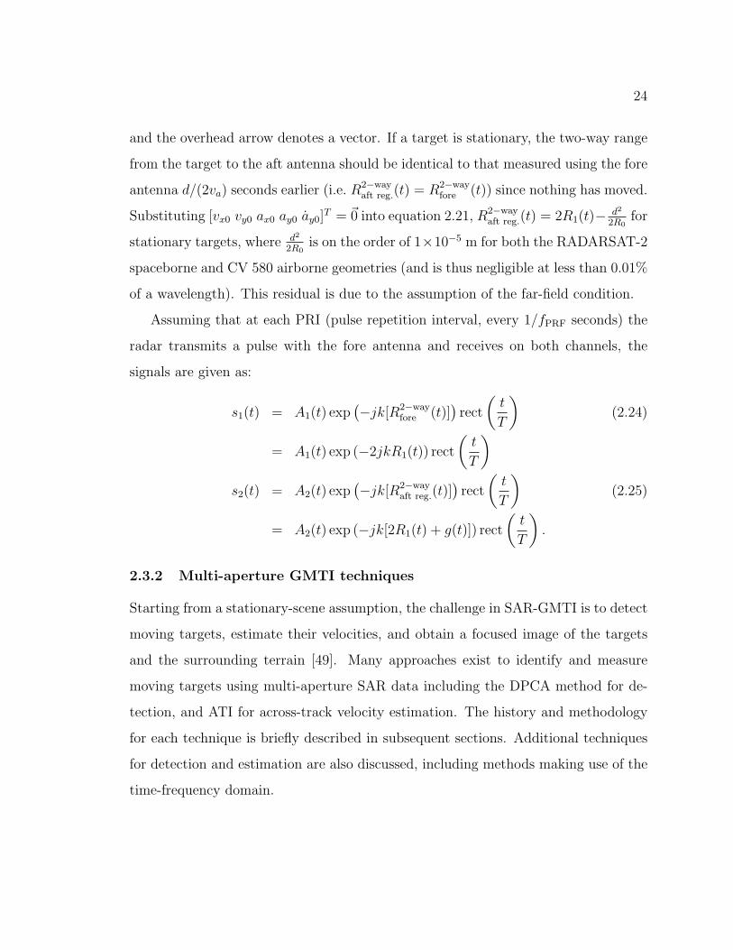
Assuming that at each PRI (pulse repetition interval, every 1/fPRF seconds) the
radar transmits a pulse with the fore antenna and receives on both channels, the
signals are given as:
s1(t) = A1(t) exp(−jk[R2−way
fore (t)])rect
(t
T
)(2.24)
= A1(t) exp (−2jkR1(t)) rect
(t
T
)s2(t) = A2(t) exp
(−jk[R2−way
aft reg.(t)])rect
(t
T
)(2.25)
= A2(t) exp (−jk[2R1(t) + g(t)]) rect
(t
T
).
2.3.2 Multi-aperture GMTI techniques
Starting from a stationary-scene assumption, the challenge in SAR-GMTI is to detect
moving targets, estimate their velocities, and obtain a focused image of the targets
and the surrounding terrain [49]. Many approaches exist to identify and measure
moving targets using multi-aperture SAR data including the DPCA method for de-
tection, and ATI for across-track velocity estimation. The history and methodology
for each technique is briefly described in subsequent sections. Additional techniques
for detection and estimation are also discussed, including methods making use of the
time-frequency domain.

25
Displaced Phase Centre Antenna (DPCA)
A common method of clutter suppression for GMTI is the displaced phase centre
antenna technique. Essentially, DPCA is the difference of the complex SAR data
from two (co-registered) channels [35]:
DPCA(t) = s1(t)− s2(t). (2.26)
In ground-based radars, stationary interference produces identical responses in
successive received pulses since neither the antenna nor the clutter moves between
measurements [39]. Thus, clutter can be rejected by subtracting consecutive mea-
surements, and any energy remaining after subtraction will be due to noise or to
moving targets. The DPCA technique is an attempt to apply this method of clutter
suppression to a radar on a moving platform.
DPCA requires the use of multiple antennae displaced along the radar platform’s
direction of travel. In classical DPCA, the speed of the radar and the physical separa-
tion distance between antennae determines the allowable PRF such that the antenna
phase centres for consecutive pulses are at the same spatial location [39]. Classical
DPCA for two antennae is demonstrated in Figure 2.4, where the radar parame-
ters are selected such that for two consecutive sampling times, the antennae provide
identical views of the illuminated field [66]. A difference image of the two channels
isolates moving targets since stationary objects will appear at the same position in
each image, whereas moving targets will have displaced in the time interval between
observations, allowing for the detection of slow moving targets that are otherwise
masked by the clutter [93].
The requirement that the antennae spatially coincide at subsequent sampling
times sets severe limitations on the PRF [21]. The PRF has a large influence on
radar performance since high PRFs allow a greater degree of oversampling and make
available a region in the Doppler domain not occupied by clutter. However, the max-
imum unambiguous swath width is inversely proportional to the PRF, and thus an
increase in the PRF reduces the available swath and increases data rates [4]. It would

26
Fore Ant.
Aft Ant.
Time = t 1
Fore Ant.
Aft Ant.
Time = t 2
Platform velocity
Platform velocity
Figure 2.4: Classical DPCA geometry, in which the phase centres of the fore and aftantennae coincide for subsequent epochs t1 and t2. Adapted from [55].
be convenient to be able to choose a PRF suitable to the speed of the targets being
imaged and to the desired swath widths of the application.
Numerous papers (e.g. [22, 60, 92]) have shown that such restrictions on the
PRF are unnecessary, as the data may be resampled in the along-track direction to
synthesize the arrangement of Figure 2.4 as long as the PRF is at or above the Nyquist
limit. This resampling process is commonly referred to as ‘channel registration’.
DPCA with two antennae can be regarded as an approximation of the optimal clut-
ter suppression achieved using STAP (space-time adaptive processing) [35]. Unlike
STAP, DPCA does not require estimation of the clutter plus noise covariance matrix
at every sample, and is thus considerably simpler and less computationally intensive
to implement. However, significant performance improvements may be achieved with
STAP including more robust clutter suppression and a mechanism for dealing with
jammers [39]. Further discussions on optimum processing using STAP may be found
in [24, 26, 35, 37, 74].
With an ideal noise-free radar and no internal clutter motion (ICM), stationary
targets and ground clutter are completely removed after DPCA [50]. However, for
real systems, clutter suppression is limited by the noise floor of the radar, ICM (from

27
time decorrelation of the clutter), fine registration errors between channels, and phase
and amplitude differences in the two receiver chains. In the complex plane, stationary
scene elements after DPCA map to a circular cluster symmetrically distributed about
the origin, i.e. with a uniform phase distribution [49]. The magnitude of these ele-
ments determines the minimum detectable velocity of scene targets, below which the
DPCA magnitude of moving targets will be indistinguishable from the noise. Moving
target detection using DPCA is further discussed in Chapter 4.
Along-track interferometry (ATI)
Along-track interferometry is another multi-aperture technique used in GMTI to de-
tect and measure target motion. Like DPCA, ATI requires multiple antennae dis-
placed in the along-track direction (i.e. the radar’s direction of travel) such that the
channels observe the same scene at different times. For a two-channel SAR system,
the ATI signal may be computed by multiplying the signal from one channel by the
complex conjugate of the second (registered) channel:
ATI(t) = s1(t)s∗2(t) = |s1(t)||s2(t)| exp
(j[ϕ1(t)− ϕ2(t)]
)(2.27)
where ∗ denotes complex conjugation, and ϕ1(t) and ϕ2(t) are the phases of the first
and second channel, respectively [49]. The phase of the ATI signal is related to the
target motion parameters (although dominated by the across-track velocity vy0) and
may thus be used to estimate vy0. For stationary terrain, the fore and aft channel
signals are identical and the ATI phase is zero.
Early advances in SAR interferometry including the history of ATI are described
in [72]. The first application of along-track interferometry was reported by Goldstein
and Zebker who used ATI to measure tidal currents by imaging the ocean surface at
multiple times [38]. An airborne system with 0.1 s between fore and aft observations
was able to measure tidal motion in the San Francisco bay area with an accuracy
of several cm/s. The technique was named ‘along-track interferometry’ due to the
arrangement of the two antennae along the flight track on a single platform. Although

28
primarily used for measuring sea surface currents in the past ([71, 72]), SAR-ATI is
also applicable for ground moving target detection and estimation [33, 49, 59].
In the interferometric SAR system concept, radar pulses are transmitted from
one antenna, and echoes are received by two antennae [72]. The phase of a single
SAR image is random, such that one cannot extract any useful information from the
phase alone [20]. However, by coherently combining the signals from two channels,
interferometric phase differences (the interferogram) may be formed. These phase
differences are related to a change in the geometric path length to the target between
observations. With knowledge of the interferometer geometry (including the antenna
separation and local incidence angle to the target), phase differences can be converted
into target/surface velocities if the antennae are separated in the along-track direction,
or converted into surface elevations if the antennae are separated in the across-track
direction (such as in traditional SAR interferometry) [72].
ATI phase is subject to several ambiguities which affect velocity estimation. The
various types of ambiguities and methods of resolving them are further discussed
in Appendix B.1. There are also several potential error sources in the ATI phase
including clutter contamination, systematic errors in the differential phase, and phase
noise. These influences on ATI are investigated in Appendix B.2.
Detection and parameter estimation
There is a wide variation in detection and estimation techniques available for GMTI
in addition to DPCA and ATI methods. A number of detection and estimation al-
gorithms have been proposed in the last decade, some of which are described below.
However, DPCA and ATI are established and relatively simple techniques, which is
why these methods were selected with which to evaluate the effects of target acceler-
ation.
Detecting a moving target requires the ability to distinguish between targets and
stationary clutter. This may be achieved by searching for targets in clutter-free
regions after some transformation of the signal data, or by enhancing the signal-

29
to-clutter ratio by suppressing the clutter [78]. As previously mentioned, STAP
techniques are available for the combined spatial-temporal filtering of data, giving
improved signal-to-clutter ratios. DPCA is the optimal linear filter for detecting a
target in homogeneous clutter [43], although an increasing amount of research is ex-
amining target detection in extremely heterogeneous clutter environments of interest
such as urban areas. Sikaneta et al. [78, 79] have proposed several target detectors
based on an eigen-decomposition of the multi-channel covariance matrix. Compar-
isons with DPCA and ATI detectors indicate improved performance with these new
eigen-based methods (including the so-called hyperbolic detector) in heterogeneous
terrain.
Estimation of the velocity vector can be performed incoherently with a single chan-
nel or coherently (with increased reliability) using two or more apertures [79]. In both
cases, range walk, azimuth displacement, azimuth smear, and defocusing effects may
provide non-coherent evidence of target motion [35]. Several multi-channel algorithms
make use of defocusing effects for estimation of along-track velocity (e.g. [36, 82]);
this method is further described in section 5.1.
Sub-aperture techniques may also be used for both single and multi-aperture ve-
locity estimation (e.g. [42, 47]). This involves the filtering of the SAR signal spectrum
into overlapping sub-bands in the azimuth direction, where each sub-band corresponds
to a portion of the radar’s azimuth illumination beam [49]. A sequence of images may
be generated, one from each sub-beam, and moving targets (whose locations shift from
one sub-beam to the next) may be identified and their velocities estimated from the
magnitude of the shift. Single aperture techniques can be used to provide a coarse
estimation of target velocity, but generally only for sufficiently bright (i.e. high RCS),
and sufficiently fast targets.
The majority of these detection and estimation techniques are applied to SAR
signals which have been range compressed. Some methods (such as certain varia-
tions of STAP or the sub-aperture techniques) make use of range compressed SAR

30
data transformed into the Doppler frequency domain using a fast Fourier transform
(FFT). However, in addition to the one-dimensional analyzes of time series or Fourier
transformed data, one can also examine the two-dimensional time-frequency (TF)
space, which may give additional insight for moving target detection and parameter
estimation. Barbarossa [5] was one of the first to propose the use of the Wigner-Ville
distribution (a TF transform) for detecting and focusing moving objects. The advan-
tages of joint time-frequency analysis are described in section 2.4.2, and additional
uses of TF analysis for investigating target acceleration are described in Chapter 7.
Various focusing algorithms for GMTI have not been described here, since gen-
erally they all involve the creation of a reference filter which is cross-correlated with
the received signal to obtain the azimuth compressed target response. The available
algorithms vary according to the approximations and assumptions made, processing
speed, and shortcuts [90]. Details on focusing targets with various motion parameters
is described in Chapter 4.
It is extremely difficult to quantify the expected accuracy in detection, parameter
estimation and focusing available using each technique. Accurate statistical models
of the clutter and target are required, although it is challenging to emulate realis-
tic heterogeneous clutter scenarios. Elaborate statistical modelling was beyond the
scope of this research, which is why expected accuracies of the detection, parameter
estimation and focusing algorithms are not provided.
2.4 Time-frequency analysis
2.4.1 Introduction
A time series representation is usually the first and most natural description of a
signal [2]. However, in order to extract the information present and use it to its full
potential, one may analyze the signal using various data representations. The Fourier
transform is the basis of a wide range of signal processing techniques used in radar
31
data analysis [85] and is given by the following:
S(f) =
∫ ∞
−∞s(t) exp(−j2πft)dt, (2.28)
where s(t) is the input signal, S(f) is the Fourier transformed signal, and f is fre-
quency. Throughout, capital letters indicate the Fourier transforms of the corre-
sponding time-domain functions. The Fourier transform indicates which frequency
components are contained in the signal, but does not reveal how frequencies change
with time [16].
In many engineering applications such as radar, sonar, and telecommunications,
the signals under consideration are known to be non-stationary, that is, their spec-
tral contents vary with time [8]. In order to derive information regarding the time
localization of spectral components, a representation of the signal data in terms of
both time and frequency is needed. To this end, the field of time-frequency analysis
was developed. In recent decades, numerous time-frequency distributions have been
put forth mapping a one-dimensional time series into a two-dimensional time and
frequency space.
2.4.2 Utility of TF analysis
Time-frequency analysis is a powerful tool which may be used in signal detection,
characterization, and processing [85]. Understanding the Doppler frequency shift
induced in SAR signal returns is essential in appreciating the utility of TF analysis
for GMTI applications.
Due to radar platform motion, each scatterer on the ground reflects an echo with a
Doppler shift proportional to the projection of the platform velocity along the line-of-
sight (the line passing through the radar and the scattering element) [6]. At broadside,
this line-of-sight velocity is zero, and thus all stationary scatterers have a zero Doppler
centroid (when observed by a side-looking radar). If a scatterer is moving however, an
additional Doppler shift is introduced which may vary from pulse to pulse, changing
the Doppler centroid and Doppler rate. The echo from the ground will possess a

32
certain Doppler bandwidth proportional to the antenna beamwidth for each pulse,
whereas the target has a narrow bandwidth for each pulse although its mean Doppler
frequency varies through time (i.e. is non-stationary) [6].
One of the most important applications of TF analysis is estimating a signal’s
instantaneous Doppler frequency, particularly in the presence of white noise, since it
allows exploitation of the different frequency behaviours between signal and noise [5].
Although the target has an extended Doppler bandwidth due to radar-target motion
during the synthetic aperture, its instantaneous bandwidth is much smaller, such that
a point target has zero instantaneous bandwidth [5]. Conversely, white noise has a
large instantaneous bandwidth, and therefore a TF transform will concentrate signal
energy along the target’s instantaneous frequency, while dispersing noise amongst
many frequencies.
In order to focus a target (i.e. perform azimuth compression) to obtain high az-
imuthal resolutions, one requires accurate knowledge of the relative motion between
the radar and the target [7]. However, in some applications, this relative motion is
not known to a sufficient accuracy (such as in airborne systems with poor inertial
sensors) or the information is not available (such as when the target is moving). In
these cases, one can estimate the motion-induced phase shift directly by integrating
the instantaneous frequency estimated within the TF domain over time. This phase
shift can then be used in a matched filter to achieve a focused image of the target
(see Chapter 7).
Another advantage of TF analysis is that one can determine the instantaneous
frequency without making any assumptions regarding its modulation through time.
Conventional autofocusing techniques compensate only linear and quadratic phase
shifts, whereas the TF approach allows estimation and compensation regardless of
the phase structure [5]. While the conventional techniques may be sufficient to focus
a target moving with constant velocity (possessing a nearly parabolic range-history),
an accelerating target with non-zero along-track acceleration or time-varying across-

33
track acceleration will have a significant cubic term in its range-history (see equation
2.11), and will benefit from TF focusing methods.
2.4.3 Time-frequency transformations
The initial stage in any TF analysis is mapping the one-dimensional time series of data
into the two-dimensional time-frequency domain. Many time-frequency distributions
(or transforms) have been developed, each with their own advantages and drawbacks.
Typically, TF transforms are separated into two categories: linear and quadratic [2].
Linear transforms are computationally efficient, but suffer from poor time-frequency
resolution. Quadratic transforms, on the other hand, have improved resolution, but
require increased computational power and introduce undesirable cross-terms if the
input signal has multiple components. The general properties of linear and quadratic
TF representations are further reviewed in subsequent sections.
Before taking the TF transform it is assumed that the radar signal data has been
compressed in range but not azimuth. As well, to avoid issues accompanying multi-
component signals and to maximize the signal-to-clutter ratio, clutter cancellation
should be performed prior to taking the time-frequency transform. The problem of
filtering radar data to cancel clutter returns has been extensively treated in the lit-
erature (e.g. [4, 26, 35, 49, 50, 94]). For dual-channel SAR-GMTI data, DPCA as
described in section 2.3.2 is commonly used for clutter cancellation. Reliable detec-
tion, focusing, and parameter estimation in the TF domain requires the preliminary
cancellation of the background clutter [4].
Linear TF transforms
Short-time Fourier transform (STFT) One of the simplest and most widely
used methods of analyzing signals in the TF domain is the STFT [5, 85]. Essentially,
the STFT breaks up a signal into small time segments, and applies the Fourier trans-
form to each piece in order to determine the frequencies present in each segment [85].
To mathematically introduce time-dependency into the Fourier transform, a short

34
time analysis window h(τ − t) centred at time t may be added [85]:
STFTs(t, f) =1
2π
∫ ∞
−∞exp(−j2πfτ)s(τ)h(τ − t)dτ, (2.29)
where f is the frequency, and s(τ) is the input signal. Multiplication by the relatively
short window h(τ − t) suppresses the signal outside a neighbourhood close to the
analyzed time t = τ , creating a local spectrum of the signal [2].
The problem is that the STFT demands a trade-off between time and frequency
resolutions [2]; a high time resolution requires a short window h(t), but high fre-
quency resolution requires a narrow bandwidth filter (i.e. a long window h(t)). This
constraint is known as the Heisenberg-Gabor inequality. Time resolution is funda-
mentally determined by the duration of the window function (denoted as ∆t), and
frequency resolution is determined by the bandwidth of the same window, lower-
bounded by the reciprocal of the window duration (denoted B where B = 1/∆t).
Thus, the time-bandwidth product (a measure of the joint TF resolution) is always
greater than or equal to one (i.e. ∆tB ≥ 1) [2].
Additional linear TF transforms Additional linear TF transforms have been
developed including the discrete or continuous wavelet transform [2], the S-transform
[85], and the so-called ‘adaptive’ time-frequency transform [15].
Instead of employing a single analysis window h(t) as in the STFT, these algo-
rithms adapt the window function to the frequency of interest. Short windows are
used at high frequencies (increasing the time resolution although degrading the fre-
quency resolution) while long windows are used at low frequencies (increasing the
frequency resolution while decreasing the time resolution). Like the STFT, these lin-
ear algorithms offer a compromise between time and frequency resolutions. Additional
details regarding these transforms are available in [2, 15, 85].
Quadratic TF transforms
The linear transforms previously discussed decompose a signal into elementary com-
ponents well-localized in time and frequency. Another approach to TF transforms

35
involves distributing the signal energy over the two variables of time and frequency
[2]. The energy of a signal s (denoted Es) can be computed by integrating the square
of the signal or its Fourier transform [2]:
Es =
∫ ∞
−∞|s(t)|2dt =
∫ ∞
−∞|S(f)|2df. (2.30)
Since the energy Es is a quadratic function of the signal, the TF energy distributions
will also be quadratic representations of the signal. The goal is find a joint TF energy
density ρs(t, f) such that
Es =
∫ ∞
−∞
∫ ∞
−∞ρs(t, f)dt df, (2.31)
and
|S(f)|2 =
∫ ∞
−∞ρs(t, f)dt (2.32)
|s(t)|2 =
∫ ∞
−∞ρs(t, f)df, (2.33)
where energy densities fulfilling the equalities in equations 2.32 and 2.33 are said to
satisfy the marginal conditions [2]. Cohen has described a general class of quadratic
TF distributions for two input signals s1(t) and s2(t) by [67]:
Cs1s2(t, f) =
∫ ∞
−∞
∫ ∞
−∞
∫ ∞
−∞
[exp(−j2πνt− j2πfτ + j2πνu)g(ν, τ) (2.34)
s1
(u +
τ
2
)s∗2
(u− τ
2
)]du dν dτ,
where C is the signal after transformation, and g(τ, ν) is a two-dimensional kernel
function. Certain choices of the kernel function will preserve the desired energy
density properties, and all distributions in Cohen’s class possess time and frequency
covariance. This guarantees that shifts in time and frequency of the signal will result
in shifts of the same amount in the TF plane [2]. Several of the most common
quadratic transforms (also called bilinear or non-linear transforms) are described in
subsequent sections.

36
Wigner-Ville distribution The Wigner-Ville distribution (WVD) is one member
of the Cohen class which is a simple yet powerful tool to analyze the Doppler history
of SAR signals [67]. Wigner originally developed the distribution for use in quantum
mechanics in 1932, and it was introduced for signal analysis by Ville sixteen years
later [85]. To obtain the Wigner-Ville distribution at a particular time, we add up
pieces made from the product of the signal at a past time multiplied by the signal at
a future time [85]. The continuous WVD of a signal is derived by using the all-pass
kernel g(ν, τ) = 1 in equation 2.34 for s1(t) = s2(t) = s(t) [67]:
WVDs(t, f) =
∫ ∞
−∞s(t +
τ
2
)s∗(t− τ
2
)exp(−j2πfτ)dτ. (2.35)
The WVD can be regarded as the TF distribution offering the best resolution in the
form of delta-pulses along the instantaneous frequency of a signal [61, 67]. Addi-
tionally, the lack of smoothing maximally conserves the information content of the
signal [67]. The WVD is always real-valued, preserves time and frequency shifts,
and satisfies the marginal properties from equations 2.32 and 2.33. A more thorough
description of the properties of the WVD is offered in [2, 6, 67, 85].
One disadvantage is that problems arise in using the WVD for signals consisting
of multiple components. Since it is a non-linear transformation, the WVD signal is
not simply the sum of the WVD of each part. For instance, given a signal composed
of two parts s1 and s2 such that
s = s1 + s2, (2.36)
the spectrum of s is the sum of the Fourier transforms of each component:
S = S1 + S2. (2.37)
However, the energy density (which is related to the WVD of the signal) is not the

37
sum of the energy densities of each part [85]:
|S|2 = |S1 + S2|2
= |S1|2 + |S2|2 + 2<{S∗1S2}
6= |S1|2 + |S2|2, (2.38)
where the <{·} operation retains the real component of its argument.
The non-linearity of the WVD emphasizes the need to remove all clutter contri-
butions to the signal prior to computing the TF transform. If clutter is not removed,
even if the signal occupies a bandwidth well-separated from the clutter, the WVD
cross-terms may obscure the target signal [6].
If the clutter is removed but the processed signal data contains multiple moving
targets, cross-terms between these signals will still be present in the WVD. Gen-
erally, detection and tracking of the instantaneous frequency for multiple targets is
completed by combining the WVD with the Hough transform [5, 15, 61]. The Hough
transform is typically used for detecting straight lines in noisy imagery, although it
may also be used to find higher-order polynomials (such as parabolas) [10] traced out
by accelerating targets in the time-frequency domain.
Discrete WVD The SAR signals to be analyzed are generally discrete, and thus
it is useful to examine the discretized version of the WVD. Re-writing the continuous
WVD from equation 2.35 as
WVDs(t, f) = 2
∫ ∞
−∞s (t + τ) s∗ (t− τ) exp(−j4πfτ)dτ, (2.39)
and assuming s(t) is sampled every ∆t seconds, we obtain the discrete-time Wigner-
Ville distribution:
WVDs(n∆t, f) = 2∆t
∞∑k=−∞
s ((n + k)∆t) s∗ ((n− k)∆t) exp(−j4πfk), (2.40)
where n and k are integers [2, 85]. The discrete WVD is periodic in frequency with
period 1/(2∆t), whereas the Fourier transform of a Nyquist-sampled signal has a

38
period twice that amount at 1/∆t. Thus, the discrete WVD may be affected by
spectral aliasing [2]. However, an important advantage of the WVD is that it allows
the recovery of a target’s instantaneous frequency history even in the case of under-
sampling. Barbarossa explains that “the TF representation prevents superposition of
spectrum replicas created by undersampling because, even if the replicas occupy the
same bandwidth, they occur at different times” [5]. Ambiguities may still exist in the
target frequency history due to undersampling, but the undersampling will not cause
overlapping signal spectra in the TF domain.
Pseudo Wigner-Ville Distribution When computing the WVD at a certain
time, the Wigner-Ville distribution weighs all signal values in the past and future
equally. In practice, we may not be able to integrate from minus to plus infinity if
we do not have knowledge of the quantity s(t + τ/2)s∗(t− τ/2) for all possible τ [2].
As well, in determining the TF distribution for a time t, we may wish to emphasize
the properties near the time of interest [85].
In these cases, a windowing function may be introduced into the WVD equation
leading to a new distribution termed the ‘pseudo WVD’ or PWVD. The PWVD is
defined as:
PWV Ds(t, f) =
∫ ∞
−∞h(τ)s
(t +
τ
2
)s∗(t− τ
2
)exp(−j2πfτ)dτ, (2.41)
where h(τ) is a window function peaked around τ = 0. This windowing operation
is equivalent to smoothing in frequency, which can improve the estimation accu-
racy of the instantaneous frequency (IF) in the presence of noise [5]. The PWVD
partially suppresses cross-terms from multi-component signals including interference
terms between the target signal and noise. However, as a consequence of the window-
ing operation many of the properties of the WVD are lost such as fulfillment of the
marginal conditions, and frequency resolution is also slightly degraded.
Additional quadratic TF distributions Beginning with the Wigner-Ville dis-
tribution, numerous quadratic TF transforms have been developed in an attempt to

39
improve the time-frequency resolution over that achievable with the STFT [52]. In
addition to the pseudo WVD, the Choi-Williams and Cone kernel transforms have
been proposed to attenuate interference effects and cross-terms in signals [2, 67].
However, like the PWVD, these techniques cause some loss in TF resolution and
increase the computational cost compared with the WVD. Other variations on the
WVD include the polynomial WVD [8] and the rotational WVD [14]. Each technique
has its respective advantages and drawbacks, and the choice of a particular transform
will depend on the requirements of each signal processing application.
Among the many time-frequency representations available, the PWVD was chosen
to transform one-dimensional time series SAR-GMTI data into the two-dimensional
time-frequency space due to the PWVD’s high time-frequency resolution, and its
ability to suppress cross-terms. Further analysis on the use of the PWVD for detecting
accelerating targets and obtaining a focused response are given in Chapter 7.

40
Chapter 3
Detection
The first step in any SAR-GMTI processing system is the detection of moving tar-
gets, afterwhich focusing and motion parameter estimation may be carried out. As
discussed in section 2.3.2, the DPCA technique is a widely-used method of clutter
cancellation, enabling users to separate stationary clutter from targets of interest.
The objective of this chapter is to describe the impact of target acceleration on
the DPCA signal of a dual-channel SAR system, and to determine its consequences
on target detection. Firstly, the mathematical expression for the DPCA response
from a moving point target is derived. The expected influence of acceleration as well
as the other motion parameters on the DPCA signal are predicted by inspection.
Next, an airborne radar-target scenario is simulated to determine the impact of
each motion parameter on the DPCA response, and to investigate the consequence
of a zero-acceleration assumption on the ability to detect moving targets. Lastly,
the DPCA algorithm is applied to experimental data to detect moving targets, and
comparisons are made to the theoretical and simulated results.
3.1 Theory
Detection is carried out using the DPCA technique because of its widespread use
in GMTI processing, its algorithmic simplicity, and because it is the optimal linear
filter for detecting a target in homogeneous clutter [43]. Further details on the DPCA
method are given in section 2.3.1. DPCA may be performed on data that have been
fully compressed (i.e. in range and azimuth dimensions) or data that have been range
compressed but are uncompressed in azimuth [79].
Each domain (azimuth compressed and azimuth uncompressed) allows for target
41
detection over a different range of across-track velocities vy0. For large vy0, sidelobe
suppression during azimuth compression suppresses the target signal, giving an ad-
vantage to using the range compressed domain. However, for low vy0 and targets
with low RCS, azimuth compression facilitates detection by concentrating the energy
spread over the entire synthetic aperture into a few pixels [79].
Although explained further in Chapter 4, azimuth compression requires a reference
filter matched to the target phase history in order to obtain a sharply focused image.
When targets are travelling with significantly non-zero velocity and/or acceleration,
the target Doppler frequencies are so mismatched to the standard processing filter
that they are not imaged at all [37]. Iterative procedures using multiple processing
filters are possible, but this requires detection and parameter estimation to be done
simultaneously. Working with range compressed data allows a separation of these two
steps.
To avoid iteration, to enable separation of the detection and estimation stages, and
to observe how the DPCA response changes over the course of a synthetic aperture,
the DPCA signal is examined in the range compressed domain only.
3.1.1 DPCA mathematical representation
The DPCA response for an accelerating point target is computed below. We begin
from the range compressed responses of the fore and aft channels (represented as s1(t)
and s2(t), respectively) given by equations 2.24 and 2.25. The one-way range to the
fore antenna from the target is given by R1(t) in equation 2.22, and the difference in
the two-way ranges to the fore and aft apertures is given by the residual term g(t) in
equation 2.23.
The DPCA response, as a function of time and vehicle dynamics, is then given by

42
the difference between the two channels:
DPCA(t) = A(t)e−2jkR1(t) − A(t)e−jk[2R1(t)+g(t)] (3.1)
= A(t)e−2jkR1(t)(1− e−jkg(t)
)= A(t)e−2jkR1(t)e−jkg(t)/2
(ejkg(t)/2 − e−jkg(t)/2
)= A(t)e−2jkR1(t)e−jkg(t)/22j sin
(kg(t)
2
),
where it has been assumed that the fore and aft antennas have identical amplitude
such that the combined target reflectivity and gain is A(t) for each channel. For
detection purposes, it is the magnitude of equation 3.1 that is of greatest interest:
|DPCA(t)| = 2|A(t)|∣∣∣∣sin [kg(t)
2
]∣∣∣∣ (3.2)
= 2|A(t)|
∣∣∣∣∣ sin[
k
2
(y0vy0
R0
d
va
+1
R0
[(vx0 − va)
2 + v2y0
(1− y2
0
R20
)+ y0ay0
](d
va
t +d2
4v2a
)
+ d(vx0 − va)
(t + d
2va
)R0
)]∣∣∣∣∣,where the third term of g(t) from equation 2.23 has been dropped due its minimal
contributions in relation to the other terms. Detection using DPCA is performed by
thresholding the magnitude signal from equation 3.2. All pixels with DPCA magni-
tudes equal to or above the threshold are potential moving targets, whereas all pixels
below are assumed to be clutter. The threshold is a subjective value and may be
chosen based on experience with the particular data set of interest, or based on a
constant false alarm rate (CFAR), in which case an accurate model of the target and
clutter probability density functions is required to choose the appropriate threshold
[32].

43
3.1.2 Analysis of the DPCA expression
The expected influence of the target motion parameters on the DPCA magnitude
may be examined using equation 3.2. Assuming that the target amplitude is rela-
tively constant over the course of the synthetic aperture, the DPCA magnitude is
determined by the g(t) function, which is the difference in the two-way path length
to the fore and registered aft apertures.
In the argument of equation 3.2 the first term (proportional to vy0) is dominant.
The second and third terms are of similar magnitudes (whose absolute values depend
primarily on the quantity (vx0 − va)) but the terms have opposite signs. This is true
for t > −d/(4va) and t < −d/(2va) since (vx0− va)2 (from the second term) is always
positive, and (vx0−va) (from the third term) is always negative for targets of interest
(i.e. targets with speeds lower than the aircraft velocity). The second and third terms
nearly cancel each other out, such that for vx0 = vy0 = 5 m/s and ay0 = 0, the absolute
value of the first term of g(t) is close to thirty times larger than the maximum sum of
the second and third terms for typical airborne scenarios, and nearly 400 times larger
than the sum for the RADARSAT-2 spaceborne scenario. Also note that the first
term in g(t) is a function of only the across-track velocity vy0, and is not dependent
upon time; this suggests that the DPCA magnitude will not be significantly affected
by target acceleration and will be relatively constant over the course of the synthetic
aperture.
As discussed above, the dominant term in the sine argument from equation 3.2
is the first term of g(t), given by ky0vy0d/(2R0va). The DPCA magnitude is thus
maximized when this term takes on a value of (2n + 1)π2, where n can be any integer
(n = 0,±1,±2, . . .). These DPCA magnitude maxima occur for:
vy0 =(2n + 1)λR0va
2y0dwhere n = 0,±1,±2, . . . . (3.3)
For a pass collected using parameters typical of Environment Canada’s CV 580 SAR
(with parameters shown in Table 3.1), the first maxima (n = 0,-1) occur at vy0 =

44
±10.2 m/s. A target imaged at the same incidence angle using RADARSAT-2 (where
λ = 0.0565 m, R0 ≈ 104 km, va = 7500 m/s, and d = 7.5 m) has maxima at ±43.9
m/s.
Similarly, the DPCA magnitude goes to zero when the sine argument takes on a
value of nπ, where n can be any integer (n = 0,±1,±2, . . .). These DPCA magnitude
minima occur for:
vy0 =nλR0va
y0dwhere n = 0,±1,±2, . . . . (3.4)
For data collected using the CV 580 SAR in the same radar-target geometry, the first
non-zero minima (n = ±1) occur at vy0 = ±20.3 m/s. The first non-zero minima
for such a target viewed from the RADARSAT-2 sensor occur at ±87.9 m/s. If it is
assumed that the antenna gain patterns, spherical propagation loss, target reflectivity,
and all other factors influencing signal amplitude have been removed from the input
fore and aft data (and thus that A(t) = 1), then the DPCA magnitudes will vary from
0 to 2, depending on the across-track velocity of the target. At the minima values,
the DPCA magnitude will be zero and thus these represent ‘blind velocities’ at which
targets cannot be detected. Thus, even if a target possesses non-zero along-track
velocity and/or any acceleration components, if its broadside velocity vy0 is close to
zero or to a blind velocity, detection may be difficult.
3.2 Simulations
To investigate how DPCA magnitude is influenced by target velocities and accelera-
tions, a MATLAB program was created to simulate airborne DPCA signal returns.
Range compressed fore and aft signals free from noise, clutter contamination, and
antenna gain patterns were generated for a radar-target geometry similar to that en-
countered using the CV 580 SAR sensor. A list of radar parameters and airborne
geometry parameters used in the simulation is provided in Table 3.1:
To minimize numerical errors, equation 2.9 was used to compute R2−wayfore (t), and

45
Table 3.1: Radar and geometry parameters for airborne SAR simulations.
Parameter Value
Pulse repetition frequency (fPRF) 642.5 HzWavelength (λ) 0.0565 mRange at broadside (R0) 10 kmIncidence angle to target (θinc) 40◦
Aircraft velocity (va) 125 m/s-3 dB antenna beamwidth (β) 3◦
Physical antenna separation distance (d) 0.54 mSynthetic aperture time (T ) 4.2 s
equations 2.15 and 2.19 were used to determine R2−wayaft reg.(t), which make use of the
far-field approximation only. Tests were conducted varying vx0, vy0, ax0, ay0, and ay0
independently and examining the DPCA magnitude over time.
3.2.1 DPCA magnitude with vy0
To begin, a target was simulated with non-zero across-track velocity vy0 varied from
-25 to 25 m/s in steps of 0.25 m/s, with all other motion parameters set to zero in
order to isolate the effects of vy0 on the DPCA magnitude. Figure 3.1 (a) shows
the sinusoidal variation of the range compressed DPCA magnitude as a function of
across-track velocity vy0 and time as predicted by equation 3.2. The magnitude is
constant for all times over the course of the synthetic aperture, and a two-dimensional
cross-section is shown in Figure 3.1 (b).
As predicted by equation 3.4, the DPCA magnitude goes to zero at vy0 = 0
and vy0 = ±20.3 m/s, and reaches a maximum at ±10.2 m/s (as anticipated from
equations 3.3 and 3.4). Note the sharp notch filter about zero-velocity, such that
targets travelling with even slight across-track velocities will possess a non-zero DPCA
magnitude.

46
(a) Variation of DPCA magnitude throughtime where the magnitudes are examined overthe course of one synthetic aperture and timet=0 corresponds to broadside time.
−30 −20 −10 0 10 20 300
0.2
0.4
0.6
0.8
1
1.2
1.4
1.6
1.8
2
vy0
(m/s)
|DP
CA
|
(b) A two-dimensional cross-sectionof figure (a).
Figure 3.1: Range compressed DPCA magnitude for a simulated target with constantvelocity vy0 varied from -25 to 25 m/s and vx0 = 0. For a particular vy0 the magnitudeis constant for all times over the synthetic aperture. Note the sinusoidal variationwith vy0 as predicted by equation 3.2, the null at vy0 = 0 m/s, and the blind velocitiesat approximately ±20 m/s.
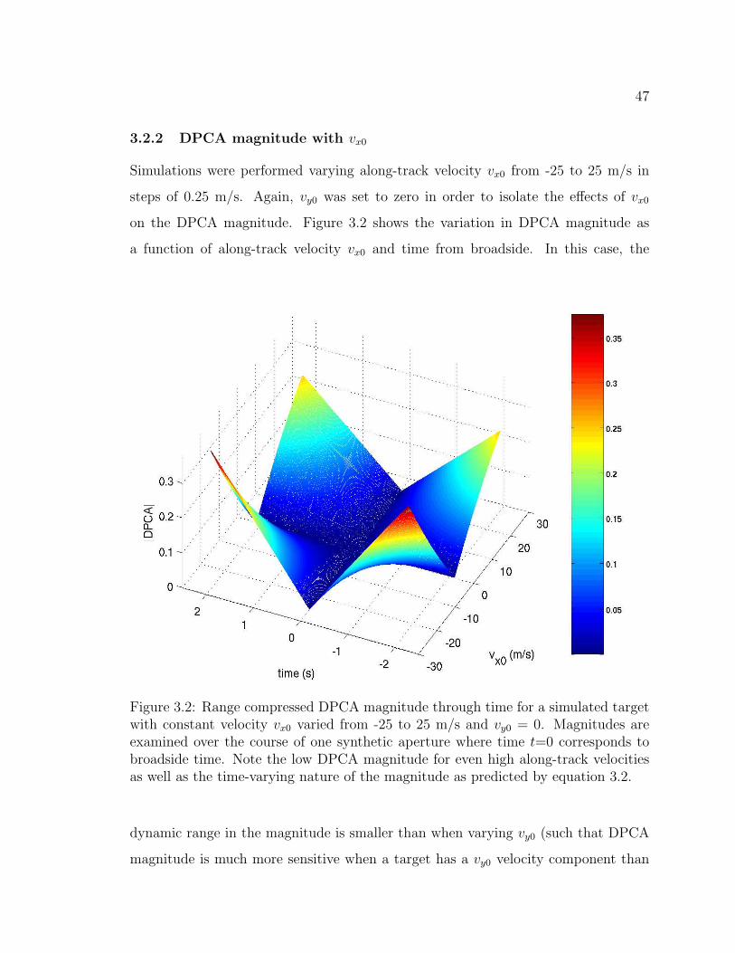
47
3.2.2 DPCA magnitude with vx0
Simulations were performed varying along-track velocity vx0 from -25 to 25 m/s in
steps of 0.25 m/s. Again, vy0 was set to zero in order to isolate the effects of vx0
on the DPCA magnitude. Figure 3.2 shows the variation in DPCA magnitude as
a function of along-track velocity vx0 and time from broadside. In this case, the
Figure 3.2: Range compressed DPCA magnitude through time for a simulated targetwith constant velocity vx0 varied from -25 to 25 m/s and vy0 = 0. Magnitudes areexamined over the course of one synthetic aperture where time t=0 corresponds tobroadside time. Note the low DPCA magnitude for even high along-track velocitiesas well as the time-varying nature of the magnitude as predicted by equation 3.2.
dynamic range in the magnitude is smaller than when varying vy0 (such that DPCA
magnitude is much more sensitive when a target has a vy0 velocity component than

48
only a vx0 component, even if the along-track velocity is relatively large). Also, note
that the DPCA magnitude varies with time from broadside for a constant non-zero
vx0 as predicted by the second and third terms in the sine argument of equation 3.2.
In many situations targets will be travelling with both along- and across-track
velocity components. Figure 3.3 displays the DPCA magnitude for a simulated target
with vy0 varied from -25 m/s to 25 m/s, but with constant vx0 = -25 m/s for all trials.
This value of vx0 was chosen since it gave the largest variation in DPCA magnitude
Figure 3.3: Range compressed DPCA magnitude through time for a simulated targetwith constant velocity vx0 = −25 m/s and vy0 varied from -25 to 25 m/s. Magnitudesare examined over the course of one synthetic aperture where time t=0 correspondsto broadside time. Note the similarities to Figure 3.1 (a) indicating that DPCA mag-nitude is dictated primarily by vy0 even in the presence of high along-track velocitiesvx0.
for the vy0 = 0 case (see Figure 3.2). However, as expected, the DPCA magnitude is

49
determined primarily by the across-track velocity vy0, with some small modulations
introduced by vx0. As predicted by equation 3.2, this modulation creates a sloping
DPCA magnitude over time which is most easily visible at the furthest ends of Figure
3.3 for vy0 = ±25 m/s. One two-dimensional cross-section of Figure 3.3 at vy0 = 1 m/s
is shown in Figure 3.4. Note that the vx0 velocity has driven the DPCA magnitude to
zero at one point in the observation interval. However, for across-track velocities with
an absolute value greater than 1.2 m/s, the DPCA magnitude is completely non-zero
over the synthetic aperture (in this specific scenario).
−2.5 −2 −1.5 −1 −0.5 0 0.5 1 1.5 2 2.50
0.1
0.2
0.3
0.4
0.5
0.6
time (s)
|DP
CA
|
Figure 3.4: Range compressed DPCA magnitude through time for a simulated targetwith constant velocities vx0 = −25 m/s and vy0 = 1 m/s. Magnitudes are examinedover the course of one synthetic aperture where time t=0 corresponds to broadsidetime. Note the changing magnitude over time, and zero magnitude at 1.5 secondsbefore broadside.
3.2.3 DPCA magnitude with ay0
The introduction of across-track acceleration ay0 has a similar effect upon DPCA
magnitude as non-zero along-track velocity vx0. Figure 3.5 displays the DPCA mag-
nitude for a simulated target with constant ay0 varied from -1 m/s2 to 1 m/s2. Again,

50
Figure 3.5: Range compressed DPCA magnitude through time for a simulated tar-get with constant across-track acceleration ay0 varied from -1 to 1 m/s2, and withvy0 = vx0 = 0. Magnitudes are examined over the course of one synthetic aperturewhere time t=0 corresponds to broadside time. Note the low DPCA magnitude foreven high across-track accelerations as well as the time-varying nature of the magni-tude as predicted by equation 3.2.

51
the magnitudes are time-varying as predicted by the second term in the sine function
of equation 3.2. The DPCA magnitude at relatively high accelerations (e.g. 1 m/s2)
rivals that of the DPCA magnitude for large along-track velocities (e.g. ± 25 m/s).
to put these values in context, an acceleration of 1 m/s2 is equivalent to adding 3.6
km/h to one’s velocity over the course of one second.
Depending on the direction of acceleration (i.e. in the positive or negative across-
track direction) and its magnitude, the vx0 and ay0 influences may nearly cancel each
other out to give a DPCA magnitude of close to zero, or they may add constructively
to increase the effective DPCA magnitude. This behaviour is due to the fact that
they both appear in the same term in equation 3.2.
As before, when across-track acceleration ay0 is added to a non-zero broadside
across-track velocity vy0, the DPCA magnitude is dominated by the vy0 term, although
the magnitude displays a slope (either positive or negative depending on the signs of
ay0 and vy0) over the observation interval.
3.2.4 DPCA magnitude with along-track acceleration ax0
Along-track acceleration ax0 has a nearly negligible effect on DPCA magnitudes. Fig-
ure 3.6 displays the DPCA magnitude for a simulated target with ax0 varied from -1
m/s2 to 1 m/s2. Note the extremely small DPCA magnitude along the z-axis when
compared to Figures 3.2 and 3.5. Equation 3.2 does not contain the ax0 variable be-
cause only second order terms of the Taylor expansion were included in its derivation.
However, to compute the DPCA target signature in each simulation, equation 2.15
was used, which does include along-track acceleration ax0 and whose only approxima-
tion is the far-field approximation (which contributes a two-way range error of only
1.5 × 10⁻⁵ metres to the estimate of R2−wayaft (t)). The low DPCA magnitudes due to
ax0 confirm that the third-order term in the Taylor expansion of the range equation
is not significant in this case, and thus equation 3.2 is an acceptable approximation
of the closed form expression for DPCA magnitude.
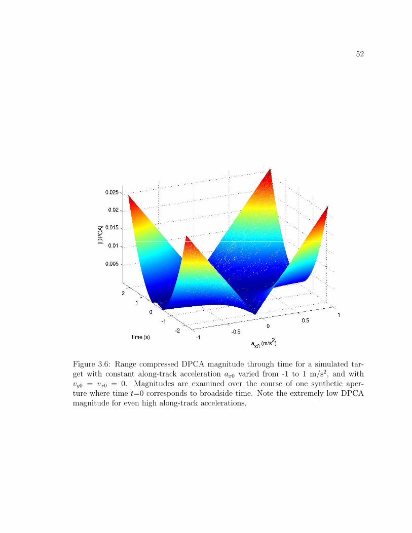
52
Figure 3.6: Range compressed DPCA magnitude through time for a simulated tar-get with constant along-track acceleration ax0 varied from -1 to 1 m/s2, and withvy0 = vx0 = 0. Magnitudes are examined over the course of one synthetic aper-ture where time t=0 corresponds to broadside time. Note the extremely low DPCAmagnitude for even high along-track accelerations.

53
3.2.5 DPCA magnitude with ay0
Similar to along-track acceleration, time-varying across-track acceleration with non-
zero ay0 has minimal impact upon the DPCA magnitude. The effects of time-varying
accelerations changing from -0.1 to 0.1 m/s3 over the course of one synthetic aperture
has effects on the DPCA magnitude of the same order as the range of ax0 tested. These
DPCA magnitude variations for changing ay0 while all other motion parameters are
set to zero are shown in Figure 3.7.
Figure 3.7: Range compressed DPCA magnitude through time for a simulated targetwith time-varying across-track acceleration with rate of change ay0 varied from -0.1to 0.1 m/s3 and with [vx0 vy0 ax0 ay0]
T = ~0. Magnitudes are examined over the courseof one synthetic aperture where time t=0 corresponds to broadside time. Note theextremely low DPCA magnitude for even high rates of acceleration change.
3.2.6 DPCA magnitude for spaceborne geometries
In addition to airborne simulations, a spaceborne scenario using parameters projected
for the RADARSAT-2 sensor was simulated. The simulation was simplistic and did

54
not take into account earth curvature, earth rotation, atmospheric propagation ef-
fects, antenna gain, clutter, or noise. However, a general idea about how velocity
and acceleration might affect DPCA magnitudes for a spaceborne geometry may be
determined using the simulation.
A list of radar and geometry parameters for the upcoming Canadian RADARSAT-
2 SAR is provided in Table 3.2.
Table 3.2: Radar and geometry parameters for RADARSAT-2 simulations [18].
Parameter Value
Pulse repetition frequency (fPRF) 1300-3800 HzWavelength (λ) 0.0555 mAltitude (H) 800 kmIncidence angle to target (θinc) 40◦
Range at broadside (R0) 1044 kmPlatform velocity (va) 7500 m/s-3 dB antenna beamwidth (β) 0.21 - 0.63◦
Physical antenna separation distance (d) 7.5 m
Note that both the azimuth beamwidth and the PRF are programmable by the
operator. In the spaceborne simulations, a PRF of 2000 Hz and a beamwidth of 0.4◦
were chosen to give a synthetic aperture time of approximately one second, with the
rest of the radar parameters set to the values given in Table 3.2.
Figure 3.8 displays the DPCA magnitude for a simulated target observed in a
spaceborne geometry with vy0 varied from -25 m/s to 25 m/s and all other motion
parameters set to zero. Although an entire period of the DPCA magnitude is not
visible for the range of simulated velocities, the sinusoidal variations in the magni-
tude and the null at zero-velocity as predicted by equation 3.2 are still visible. One
advantage of the spaceborne scenario is that there are no DPCA blind speeds at the
target velocities of interest.

55
Figure 3.8: Range compressed DPCA magnitude through time for a simulated targetobserved in a spaceborne geometry with across-track velocity vy0 varied from -25 to25 m/s. Magnitudes are examined over the course of one synthetic aperture wheretime t=0 corresponds to broadside time. Note the similarities to Figure 3.1, includingthe sinusoidal variation with vy0 as predicted by equation 3.2, and the null at vy0 = 0m/s.

56
Targets with non-zero across-track acceleration ay0 were also simulated for the
spaceborne case. Figure 3.9 displays the DPCA magnitude for a simulated target
with constant ay0 varied from -1 m/s2 to 1 m/s2. In the spaceborne case the geometry
Figure 3.9: Range compressed DPCA magnitude through time for a simulated targetobserved in a spaceborne geometry with constant across-track acceleration ay0 variedfrom -1 to 1 m/s2, and with vy0 = vx0 = 0. Magnitudes are examined over the courseof one synthetic aperture where time t=0 corresponds to broadside time. Note thelow DPCA magnitudes compared to the airborne case of Figure 3.5.
is such that vx0 and ay0 have even less of an influence on the DPCA magnitude than
in the airborne scenario. For instance, comparisons between Figures 3.5 and 3.9
reveal peak DPCA magnitudes twenty times lower in the spaceborne case than in the

57
airborne scenario. This is due to differences in the d/va factor multiplying vx0 and ay0
in equation 3.2, which is approximately four times smaller in the spaceborne scenario.
Additionally, the synthetic aperture time is approximately four times shorter in the
spacebased case, which further decreases the peak DPCA magnitudes.
3.2.7 Analysis of DPCA magnitude simulations on target detection
As discussed in previous sections, DPCA magnitudes may be used in combination
with a decision rule or threshold to separate pixels containing moving targets from
clutter. Following the initial target detection, the target may be tracked through
azimuth for the duration of the synthetic aperture to extract the track for further
processing including focusing and parameter estimation.
Detection and tracking of targets with non-zero across-track velocity vy0 is rela-
tively straightforward as long as targets are not travelling at a blind velocity. The
notch in the sine function about zero-velocity in Figure 3.1 is quite sharp, such that
targets travelling with even small across-track velocities will have non-zero DPCA
magnitudes that will remain constant across the observation interval. However, in
the presence of residual clutter and high noise levels, the DPCA magnitude threshold
for detection must be raised significantly above zero, and thus the detection of slow-
moving targets or targets moving close to the blind velocities remains challenging
[41].
The time-varying nature of the DPCA range compressed magnitudes as observed
in the simulations has implications on the effectiveness of target detection and track-
ing through azimuth. Non-zero DPCA magnitudes are observed in Figure 3.2, such
that given sufficiently low noise and significant clutter suppression, one can detect
targets in the range compressed data moving completely in the along-track direction.
However, the time-varying nature of the magnitudes across the observation interval
may make it difficult to track a target through azimuth which is travelling only with
a vx0 component. The peaks in the DPCA magnitude signal occur well away from

58
broadside, and tracking the target over the entire observation interval is not possible
as the DPCA signal magnitude fades to zero as the time approaches broadside. Addi-
tionally, because the peak responses from targets moving along-track occur at the far
edges of the beam, their DPCA magnitudes may be suppressed due to the antenna
gain pattern, making the targets even more difficult to discern from the background
residual clutter.
These same observations apply to a target moving with across-track acceleration
ay0 and across-track velocity vy0 = 0 at broadside. However, although the scenario
of targets moving completely along-track may be quite common, a target with zero
across-track broadside velocity and non-zero across-track acceleration is somewhat
of a pathological case. It is difficult to conceive of a plausible situation in which
this would occur, although the simulations with zero vy0 were useful in isolating the
influence of ay0 on DPCA magnitude.
In the presence of non-zero vy0 and large ay0 or vx0, it is likely that a target
will be detected using the DPCA magnitude, but it may be difficult to extract the
entire target track. The sloping DPCA magnitude presents a problem at across-
track broadside velocities vy0 very close to the the blind velocities (within 1.2 m/s
of the blind velocities for the simulated airborne scenario). In these cases, the slope
introduces a null in the DPCA magnitude, which will create a break in the extracted
target track. If the DPCA detection threshold is sufficiently low however, the gap in
the extracted track will be small and may be bridged using a moving average filter
to connect track segments. This type of approach was used in tracking targets in
experimental data, as will be described in section 3.3.1.
Even large values of along-track acceleration ax0 and across-track acceleration
rates ay0 did not have an noticeable impact on DPCA magnitudes, and thus would
not hamper detection as long as an across-track vy0 component is present. Simula-
tions of the RADARSAT-2 spaceborne scenario revealed relatively small modulations
introduced by vx0, ax0, ay0, and ay0 on the DPCA magnitude when compared to the

59
airborne case. This suggests that time-varying DPCA magnitudes will be even less
of a concern for spaceborne GMTI sensors.
In summary, theory and simulations have shown that the addition of target accel-
eration will not severely deteriorate target detection using DPCA; it is expected that
most targets will be detected and tracked for the entire observation interval if they
possess an across-track velocity component away from the blind velocities.
3.3 Experimental results
Having described the theory and conducted simulations of detection by DPCA, it
was desired to examine target detection using experimental data. Dual-channel SAR
data were collected during an experiment conducted at Canadian Forces Base (CFB)
Petawawa with the Environment Canada CV 580 C-Band SAR in November of 2000.
Three control targets were used in the experiment, each of which was equipped with a
trihedral corner reflector and a GPS (Global Positioning System) receiver. The corner
reflector increases target reflectivity (RCS) such that the target is more visible in the
radar imagery, and the GPS data allows precise determination of the target position
and velocities at all times. Two targets (dubbed ‘Juliet’ and ‘Delta’) were rail cars
moving along a rail track, and the third target (called ‘Convoy’) was a vehicle driving
along a gravel road. All targets attempted to maintain constant speed during the
synthetic aperture of the radar. Eight passes were flown from four different aspect
angles with a total of twenty-two control target tracks to analyze. Further descriptions
and images of the experimental set up are given in Appendix A and [49]. Appendix
A also outlines the pre-processing performed on the data.
3.3.1 Detection and tracking algorithm
A detection and tracking algorithm in the range compressed domain using the DPCA
technique for clutter suppression was employed to extract and store the track of
each target. The algorithm was developed by Christoph Gierull [36], although slight

60
modifications were made by this author to ease input and calculation of the required
parameters, and to set algorithmic thresholds appropriate for the data set.
The program (designed for CV 580 SAR data) accepts range compressed fore and
aft data chips as input as well as a number of input parameters including aircraft
velocity (va), near range to the first pixel of the data chips, aircraft altitude, and
fPRF/va ratio. The algorithm assumes that internal clutter motion is insignificant,
and that the range pixel is large enough (or the target size is small enough) such
that the energy of each target is concentrated in a single range cell at each azimuthal
time. Whereas many detection techniques are applied in the azimuth compressed
domain, this algorithm works with only range compressed data, which is not biased
against high-velocity targets for detection, and allows a separation of the detection
and estimation stages as described in section 2.3.2. The algorithm is described below,
with images from one pass of the Delta target given to illustrate the detection process.
The algorithm begins with the computation of several magnitude maps. Firstly,
the average magnitude of both channels is determined as
|s(t)| = |s1(t)|+ |s2(t)|2
, (3.5)
where s denotes the mean value of s. Next, the DPCA magnitude is computed
as |DPCA| = |s1(t) − s2(t)|. Both magnitude maps are then convolved with a
one-dimensional moving average (i.e. lowpass) filter in azimuth to smooth the data
(thereby decreasing noise), and then each pixel is normalized by dividing it by the
mean magnitude value. The smoothed DPCA magnitude image may also be referred
to as the nLooks DPCA map, where nLooks represents the length of the lowpass filter.
An example of the DPCA magnitude image before and after smoothing is shown in
the first two columns of Figure 3.10 for one pass of the Delta target.
Next a two-step power detector is applied to the convolved and normalized mag-
nitude maps. Potential target pixels must meet the following criteria:
10 log10 |DPCA| > 2 dB AND 10 log10
|s(t)||DPCA|
< −2 dB, (3.6)

61
|DP
CA
|
rang
e
azimuth
180
190
200
4000
5000
6000
7000
8000
9000
|DP
CA
| sm
ooth
ed
rang
e18
019
020
0
4000
5000
6000
7000
8000
9000
|DP
CA
| afte
r mas
king
and
seco
nd s
moo
thin
g
rang
e18
019
020
0
4000
5000
6000
7000
8000
9000
rang
e
Det
ecte
d tra
ck
180
190
200
4000
5000
6000
7000
8000
9000
0102030405060708090
Fig
ure
3.10
:Fou
rst
ages
ofth
eta
rget
det
ection
and
trac
kin
gpro
cess
oper
atin
gin
the
range
com
pre
ssed
dom
ain.
Fro
mle
ft:
DP
CA
mag
nit
ude
imag
e,D
PC
Aim
age
smoot
hed
wit
ha
20pix
elm
ovin
gav
erag
efilt
er,th
resh
olded
DP
CA
map
hea
vily
smoot
hed
wit
ha
750
pix
elm
ovin
gav
erag
efilter
(to
bri
dge
gapsin
the
trac
k),
final
det
ecte
dtr
ack
afte
rcl
ust
erin
gov
erla
idon
smoot
hed
DP
CA
imag
e.

62
where the two thresholds (2 dB and -2 dB) may be changed if the user so desires. The
first condition ensures that the target has a significant non-zero DPCA magnitude.
The second condition examines the ratio of power before and after the application
of DPCA. This is done to eliminate bright, stationary scatterers (clutter discretes
such as buildings) whose signals have been significantly suppressed by DPCA, even
though the DPCA magnitudes remain relatively large compared to other clutter. This
approach was also suggested by White et al. [92].
The next step is to further smooth the detected pixels in order to bridge any
gaps in the track using a second (and much longer) moving average filter. The first
threshold from equation 3.6 is then reapplied, and a binary detection map is created
by assigning pixels as moving or not. The third column in Figure 3.10 demonstrates
the thresholded, heavily smoothed target DPCA image. The binary detection map
is then applied as a mask onto the nLooks DPCA map to extract only the pixels of
interest for tracking.
For each pulse (i.e. each range line), the local maxima in the masked DPCA image
are stored. This reduces a target track spread out across multiple range cells (perhaps
due to sidelobes) to a target track only a single range cell thick.
The next step is to identify separate target tracks in the binary detection image
(i.e. to cluster all detections into a finite number of tracks). A target track is permitted
to jump from one range cell to a neighbouring range cell, but is not allowed to have
any gaps in azimuth, since the long moving average filter should have bridged any
azimuthal gaps.
The tracking algorithm works by systematically stepping through all azimuthal
slow times and all range lines in two nested loops. When the first detection is reached,
a new cluster is created if a second detection is found in the next azimuth slow time
and in a nearby range cell. Clusters are grown by comparing each detection with
detections at the previous azimuth time. If a cluster already exists in a nearby range
cell, the new pixel is added to the cluster. If a ‘detected’ pixel cannot find a nearby

63
detection in the past azimuth time, a new cluster is created. Finally, any target tracks
consisting of too few pixels are considered false alarms and are removed. Ideally, one
should be able to track a target through the entire synthetic aperture time, which is
on the order of 2700 pixels for the CV 580 SAR azimuthal pixel spacing, beamwidth,
and ranges.
The program requires several thresholds to be set including the size of the various
moving average filters, the power detector thresholds, the minimum number of con-
secutive detections in azimuth (slow time) required to be considered a genuine target
track, and the maximum jump in range bins permitted when clustering target pixels
into a single track (generally set to one pixel). Some of these thresholds are data
specific, and they were set using educated guessing and trial and error. In practice
they will be calculated as CFAR thresholds, although this lies beyond the scope of
this thesis.
Once set, all thresholds were kept constant for processing the eight passes of the
Petawawa 2000 data, except the maximum jump in range bins, which had to be re-
laxed to two pixels to ensure the continuity of two detected tracks. In these instances
target segments were clustered separately due to range jumps in the maximum mag-
nitude of the DPCA target track of more than one pixel.
3.3.2 Analysis and results of experimental detections
The detection and tracking algorithm described in section 3.3.1 was applied to data
patches containing each of the twenty-two control targets. From the GPS data and
aircraft headings, it was known that all targets had non-zero across-track velocity
components, and thus it was expected from the theory and simulation results (see
section 3.2.7) that all targets would be detected in the DPCA magnitude imagery.
As expected, all twenty-two targets were detected and successfully tracked through
azimuth despite the presence of along-track velocity or any type of acceleration com-
ponents. It was mentioned earlier that the controlled movers attempted to maintain

64
a constant velocity during data collection. However, miscommunication between the
aircraft and the control vehicles sometimes resulted in them being imaged during
times of non-constant velocity and even during non-constant acceleration.
Unfortunately, it is difficult to verify the true acceleration of the control targets
over time since GPS data were only collected at a data rate of 0.5 Hz, and thus
updates are available only every two seconds. A target is illuminated by the -3
dB beamwidth of the antenna for approximately 4 seconds in the CV 580 geometry
(taperture ' R0β/va where range to the target R0 can be approximated as 10 km, the -3
dB beamwidth β as three degrees, and the aircraft velocity va as 125 m/s). However,
when targets are mounted with a corner reflector, the available synthetic aperture
time may significantly increase due to the extremely strong sidelobe responses that
are not completely suppressed by the fading antenna gain pattern. For instance, the
Delta target from one pass was tracked for 8.9 seconds through azimuth time.
Even with this extended illumination time however, accurately capturing the ac-
celeration time-history over the course of the target observation period is not possible
due to the low sampling rate of the GPS measurements. However, one can get a rough
idea of whether the target was maintaining a constant velocity or not by examining
the GPS velocity measurements over time. Technical specifications [58] cite RMS
(root mean square) accuracies of 0.03 m/s in velocities computed from differentially
processed GPS data such as that available for the experimental data set, and therefore
small changes in target velocity over the synthetic aperture should be visible.
The GPS velocities of the controlled movers during one pass are shown in Figure
3.11 in the vicinity of broadside time t=0 (where the GPS times were loosely synchro-
nized to the radar azimuth times, although there may be errors of several seconds).
Observe the acceleration and deceleration occurring in each case, although the speeds
have not been separated into along- and across-track components. The presence of
acceleration is not surprising since the Delta and Juliet targets were on relatively
short tracks, and thus required significant acceleration to bring them up to the de-

65
−6 −4 −2 0 2 4 65.5
5.55
5.6
5.65
5.7
5.75
5.8
5.85
5.9
5.95
time (s)
GP
S v
eloc
ity (m
/s)
(a) GPS velocities for Juliet.
−6 −4 −2 0 2 4 69
9.5
10
10.5
11
11.5
12
time (s)
GP
S v
eloc
ity (m
/s)
(b) GPS velocities for Delta.
−6 −4 −2 0 2 4 618.3
18.35
18.4
18.45
18.5
18.55
18.6
18.65
time (s)
GP
S v
eloc
ity (m
/s)
(c) GPS velocities for Convoy.
Figure 3.11: Variation of target velocity (obtained from GPS) through time in thevicinity of broadside time t=0 for a single pass.
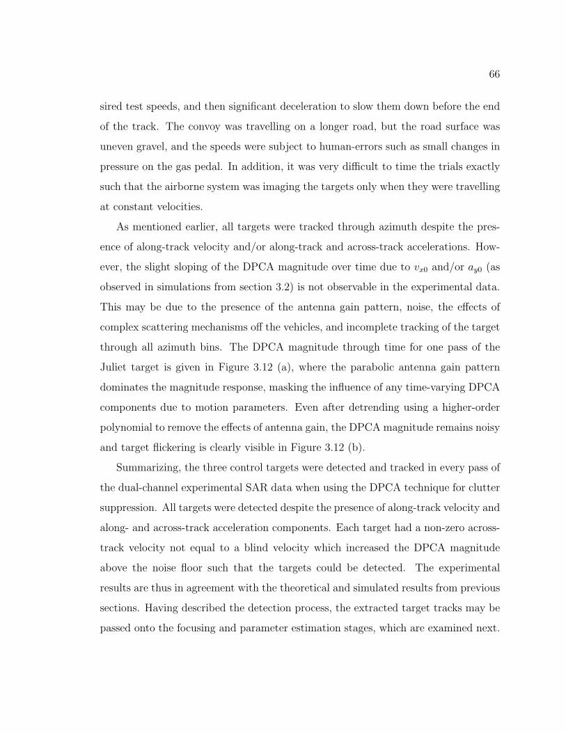
66
sired test speeds, and then significant deceleration to slow them down before the end
of the track. The convoy was travelling on a longer road, but the road surface was
uneven gravel, and the speeds were subject to human-errors such as small changes in
pressure on the gas pedal. In addition, it was very difficult to time the trials exactly
such that the airborne system was imaging the targets only when they were travelling
at constant velocities.
As mentioned earlier, all targets were tracked through azimuth despite the pres-
ence of along-track velocity and/or along-track and across-track accelerations. How-
ever, the slight sloping of the DPCA magnitude over time due to vx0 and/or ay0 (as
observed in simulations from section 3.2) is not observable in the experimental data.
This may be due to the presence of the antenna gain pattern, noise, the effects of
complex scattering mechanisms off the vehicles, and incomplete tracking of the target
through all azimuth bins. The DPCA magnitude through time for one pass of the
Juliet target is given in Figure 3.12 (a), where the parabolic antenna gain pattern
dominates the magnitude response, masking the influence of any time-varying DPCA
components due to motion parameters. Even after detrending using a higher-order
polynomial to remove the effects of antenna gain, the DPCA magnitude remains noisy
and target flickering is clearly visible in Figure 3.12 (b).
Summarizing, the three control targets were detected and tracked in every pass of
the dual-channel experimental SAR data when using the DPCA technique for clutter
suppression. All targets were detected despite the presence of along-track velocity and
along- and across-track acceleration components. Each target had a non-zero across-
track velocity not equal to a blind velocity which increased the DPCA magnitude
above the noise floor such that the targets could be detected. The experimental
results are thus in agreement with the theoretical and simulated results from previous
sections. Having described the detection process, the extracted target tracks may be
passed onto the focusing and parameter estimation stages, which are examined next.
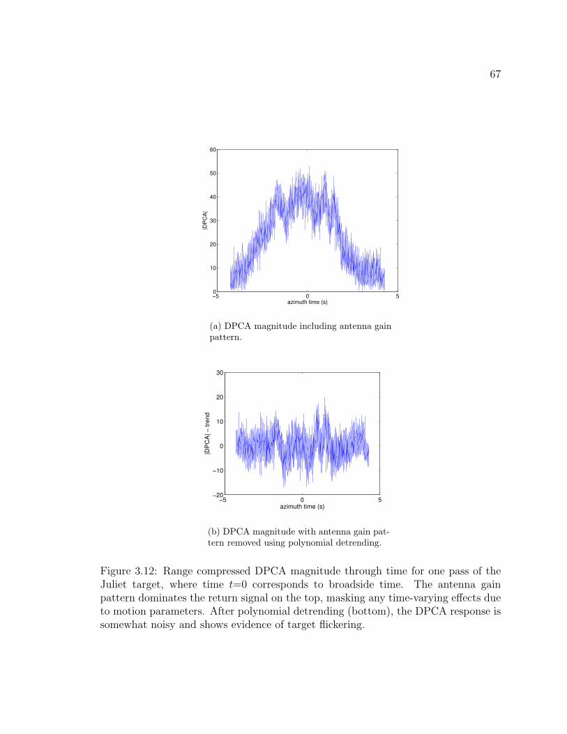
67
−5 0 50
10
20
30
40
50
60
azimuth time (s)
|DP
CA
|
(a) DPCA magnitude including antenna gainpattern.
−5 0 5−20
−10
0
10
20
30
azimuth time (s)
|DP
CA
| − tr
end
(b) DPCA magnitude with antenna gain pat-tern removed using polynomial detrending.
Figure 3.12: Range compressed DPCA magnitude through time for one pass of theJuliet target, where time t=0 corresponds to broadside time. The antenna gainpattern dominates the return signal on the top, masking any time-varying effects dueto motion parameters. After polynomial detrending (bottom), the DPCA response issomewhat noisy and shows evidence of target flickering.

68
Chapter 4
Focusing
To reconstruct a range compressed moving target signal into a focused target image,
azimuth compression of each receiver channel is required. Focusing (also known as
azimuth compression) was briefly discussed in section 2.1. Details on focusing theory
and its application to simulated and experimental data are presented here.
The objective of this chapter is to describe the impact of acceleration on the fo-
cused response from a point target in the fore and aft channels, and the consequences
of a zero-acceleration assumption. Focusing is discussed prior to motion parameter
estimation, since the estimation algorithms discussed in subsequent chapters imple-
ment azimuth compression in their solution. Airborne geometries are assumed for
the majority of the theoretical and simulated cases, although the application of the
results to spaceborne scenarios are described for certain computations. Theory and
simulations are combined since it was not possible to derive a closed form expression
for the azimuth compressed response when there are higher-order terms in the phase
history of the target signal, although we can observe the response in simulations.
4.1 Theory and simulations
Azimuth compression is achieved by constructing a reference filter with a phase history
matched to that of the received signal, and then cross-correlating this reference with
the target signal [29]. This operation is called ‘matched filtering’. Thus, for the ith
(either fore or aft) channel,
Ii(t) =1
T
∫ ∞
−∞si(t + τ) r∗i (τ) dτ, (4.1)
where Ii(t) is the focused signal for the ith channel, si(t) is the received target signal
(after range compression), ri(t) is the reference signal, and ∗ denotes complex conju-

69
gation. Duration T is the maximum usable synthetic aperture time, often taken as
the -3 dB azimuthal beamwidth. A division by T is inserted into equation 4.1 such
that the focused signal is unitless.
Gierull and Livingstone note that the quality and focus of an image is constrained
by noise and noise-like processes, by knowledge of the relative motion between the
radar and the target, and by the fidelity of the processor in applying the matched
filter [35]. The noise-like processes may include additive thermal noise of the radar
and multiplicative noise (such as oscillator phase noise) caused by real hardware
and sampling limitations. Further details on the SAR image formation process and
algorithms for focusing stationary targets are provided in [9, 13, 29, 73, 87].
The azimuth compressed signal after matched filtering is derived in subsequent
sections for both stationary and moving targets. The impact of a mismatch between
the reference and target phase histories due to uncompensated target motion is also
examined.
Matched filtering requires knowledge of the two-way ranges to the fore and aft
apertures. Assuming an airborne radar-target geometry identical to that described in
section 2.3.1, the two-way ranges R2−wayfore (t) and R2−way
aft reg.(t) (after channel registration)
were derived using a third-order Taylor series expansion of the range equation, and
are given by equations 2.17 and 2.21, respectively.
4.1.1 Focusing a stationary target
If a target is stationary (i.e. the target position has no time dependence), then the tar-
get in both channels may be focused using a stationary world matched filter (SWMF):
rSWMF(t) = exp
(−2jk
[v2
a
2R0
t2])
rect
(t
T
), (4.2)
where rSWMF(t) represents the reference signal whose range history is derived by set-
ting all target velocities and accelerations to zero in equation 2.22, and removing the
first R0 term (which will simply add a constant phase term). The target signal s(t)

70
from equation 2.12 for both channels is equivalent to rSWMF(t) except that s(t) con-
tains a magnitude factor A(t) and a constant phase term exp(−2jkR0). Performing
the cross-correlation in equation 4.1 and assuming that the antenna gain is removed
such that the magnitude is no longer a function of time and is identical in both chan-
nels (i.e. Ai(t) = A), then the focused stationary target image (for both the fore and
aft channels for a target with broadside position described in section 2.3.1) is given
by:
I(t) =A (T − |t|)
Texp (−2jkR0) sinc
(kv2
a(T − |t|)R0
t
)rect
(t
2T
), (4.3)
where sinc(x) = sin x/x.
The maximum of I(t) occurs when the argument of the sinc function is zero, and
thus the peak response of the focused target appears at broadside time t=0 which
coincides with the true position of the scatterer. The first zeroes of I(t) occur when
the argument of the sinc function is ±π. Solving equation 4.3, this occurs at
t =±T ∓
√T 2 − 2λR0
v2a
2. (4.4)
For radar parameters and an airborne geometry typical of Environment Canada’s CV
580 SAR (see parameters listed in Table 3.1), this translates to nulls at ±0.54 m or
a -3 dB width of 0.47 m. This is much finer than the achievable azimuth resolution
of the CV 580 system (approximately 0.85 m [46]) since the real system has noise,
system losses, and significant energy loss of the target signal due to the antenna gain
patterns and weighting functions used for sidelobe suppression.
4.1.2 Focusing a moving target with a SWMF
The SAR imaging of moving targets and the target response when processed using
conventional SAR-imaging techniques was first treated by Raney [62]. He found that
the response from a moving target is highly dependent upon the target dynamics,
such that the image becomes smeared in range and shifted in azimuth due to across-
track velocity, and smeared in azimuth due to along-track velocity and across-track

71
acceleration. Since that time, numerous papers (e.g. [17, 20, 35, 41, 67, 80, 90, 93])
have examined the influence of target motion upon the processed SAR response both
theoretically and experimentally. A summary of these effects and their causes is
given below by the theoretical development of the SWMF response to a moving
target signal. Oftentimes, target responses from badly mismatched reference signals
may not be discernible in the SAR image due to the presence of clutter, increasing
the difficulty of detection and subsequent parameter estimation. However, in this
treatment, simulations are carried out without any added clutter or noise.
If the stationary world reference signal from equation 4.2 is used to focus the
range compressed signal s1(t) received by the fore antenna of an accelerating target,
the phase history is not matched. Let the target signal be modelled as s1(t) =
A exp(−jkR2−wayfore (t))rect(τ/T ), where R2−way
fore (t) is given in equation 2.17. Then, the
azimuth compressed image is given by the following:
I1(t) =A
T
∫ ∞
−∞exp
(−2jk
[R0 +
y0vy0
R0
(t + τ) (4.5)
+1
2R0
((vx0 − va)
2 + v2y0
(1− y2
0
R20
)+ y0ay0
)(t + τ)2 + O((t + τ)3)
])· exp
(+2jk
[v2
a
2R0
τ 2
])· rect
(t + τ
T
)rect
( τ
T
)dτ,
where O(t3) represents all terms of third-order and above. Pulling all terms not a
function of τ out of the integration we have:
I1(t) =A
Texp
(− 2jk
[R0 +
y0vy0
R0
t (4.6)
+1
2R0
((vx0 − va)
2 + v2y0
(1− y2
0
R20
)+ y0ay0
)t2 + O(t3)
])
·∫ ∞
−∞exp
(− 2jk
[y0vy0
R0
τ +1
2R0
((vx0 − va)
2 + v2y0
(1− y2
0
R20
)+ y0ay0
)(2tτ + τ 2)
+ O(t2τ + tτ 2 + τ 3)
])exp
(+2jk
[v2
a
2R0
τ 2
])rect
(t + τ
T
)rect
( τ
T
)dτ.
The above equation cannot be solved analytically because there is no closed form
expression for the definite integral of exp(τ 2) and exp(τ 3) with respect to τ . However,

72
this integration may be performed numerically using a software program such as
MATLAB; since sampled radar signals are discrete rather than continuous with time
in any case, this representation is justified. A simulator initialized with radar and
geometry parameters similar to those encountered using the CV 580 airborne system
(see Table 3.1) was created within MATLAB to determine the influence of various
target motion parameters on focusing. Each velocity and acceleration component is
treated separately in order to isolate the effects of each parameter on target focusing.
The response from a stationary point target is given as a reference in the top
portion of Figure 4.1. The response is not an ideal sinc function due to the fact that
the sampling times (determined by the PRF) are not coincident with the zeros of
the sinc function. As mentioned in section 4.1.1, the -3 dB width of the peak mag-
nitude response is 0.47 m. This peak is centred about azimuth position x=0 metres
corresponding to a broadside time of t=0 seconds. Using results from MATLAB sim-
ulations, the properties of moving target signals processed using a stationary world
matched filter are examined below.
Focusing with across-track velocity vy0
When a target is given a non-zero across-track velocity component, the peak magni-
tude decreases in the azimuth compressed signal and its azimuth location shifts with
respect to the stationary case, although its -3 dB width increases only slightly. For
constant velocity, let vx = vx0 and vy = vy0 for the entire observation period. The
effects of vy on focusing are evident in the middle frame of Figure 4.1, which shows
the magnitude response from a simulated non-accelerating point target with vx = 0
and vy = 1 m/s.
These effects are perhaps most easily understood in the time-frequency domain
(see section 2.4 for an introduction to time-frequency analysis). A stationary world
matched filter and moving target signal are depicted in the time-frequency domain
in Figure 4.2. Azimuth compression consists of convolving the reference (SWMF)
signal with the target signal, with the maximum response occurring when there is the
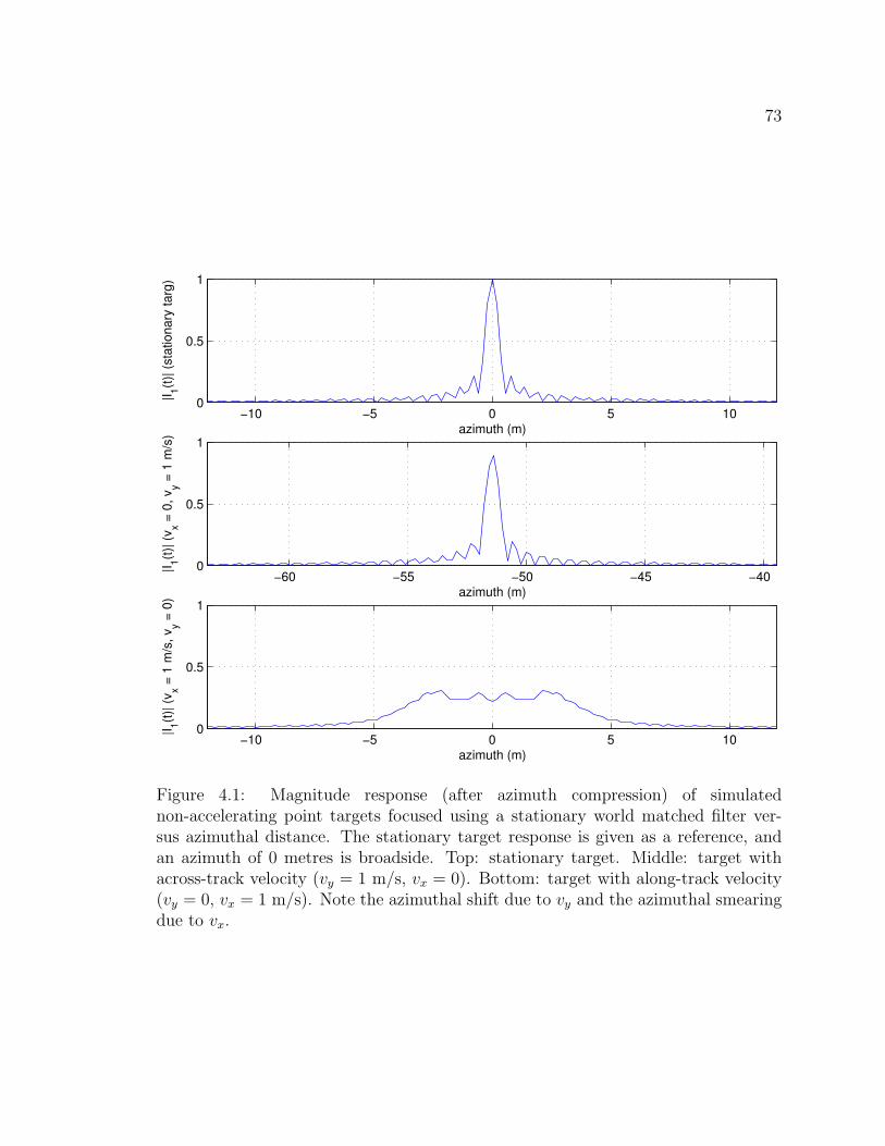
73
−10 −5 0 5 100
0.5
1
azimuth (m)
|I 1(t)| (
stat
iona
ry ta
rg)
−60 −55 −50 −45 −400
0.5
1
azimuth (m)
|I 1(t)| (
v x = 0
, vy =
1 m
/s)
−10 −5 0 5 100
0.5
1
azimuth (m)
|I 1(t)| (
v x = 1
m/s
, vy =
0)
Figure 4.1: Magnitude response (after azimuth compression) of simulatednon-accelerating point targets focused using a stationary world matched filter ver-sus azimuthal distance. The stationary target response is given as a reference, andan azimuth of 0 metres is broadside. Top: stationary target. Middle: target withacross-track velocity (vy = 1 m/s, vx = 0). Bottom: target with along-track velocity(vy = 0, vx = 1 m/s). Note the azimuthal shift due to vy and the azimuthal smearingdue to vx.

74
time
SWMF
azimuth bandwidth (PRF)
+ PRF/2
- PRF/2 Target signal
synthetic aperture length (T)
frequency
0 > y v
t img
Figure 4.2: Example time-frequency representation of a stationary world matchedfilter (SWMF in solid blue) and a target moving in the across-track direction withvy > 0 m/s (in dotted red). During azimuth compression the SWMF (of length Tseconds) is convolved with the the target signal, giving a focused peak at a timetimg < 0.

75
greatest overlap between the two signals. If one imagines the reference filter being
dragged along the time-axis, and that the product of the reference and target signals is
summed at each time instance, the azimuth time of greatest overlap occurs at a value
less than zero. This is also the azimuth time at which the target is focused, which is
significantly offset from broadside for even small across-track velocities. The offset for
vy = 1 m/s is 0.4 s, translating to -51 m off-broadside, as shown in the middle frame
of Figure 4.1. This azimuthal shift may be computed theoretically by determining
the time at which the Doppler is zero (see equation 4.7), or by computing the peak
location of an approximation of equation 4.6, which has a closed form solution for the
compressed target response (see section 4.1.3).
The peak magnitude response decreases with increasing target across-track veloc-
ity magnitudes. Again, this can be visualized in the time-frequency domain where the
target signal is offset along the frequency axis from the reference signal because of a
different Doppler centroid value. During azimuth compression, the SWMF is dragged
across the time-axis. Even at maximal overlap the two signals do not completely
coincide, and thus some target energy is not captured.
Due to a finite azimuth bandwidth (equal to the PRF), parts of the target energy
may be aliased such that the TF history wraps to fall within a frequency range of
±PRF/2 (see Figure 4.3). The point at which the TF history wraps is dependent
upon the target motion parameters (both along- and across-track velocities and ac-
celerations, which determine the Doppler rate and Doppler centroid) as well as the
radar parameters (including azimuthal beamwidth and PRF, which determine the
synthetic aperture length and the total available bandwidth). In the case of wrap-
ping, a secondary peak may appear at another azimuth time (other than timg), which
may create ghosting and lead to ambiguities if its magnitude rivals that of the first
peak. These issues are discussed further in Appendix B.1.
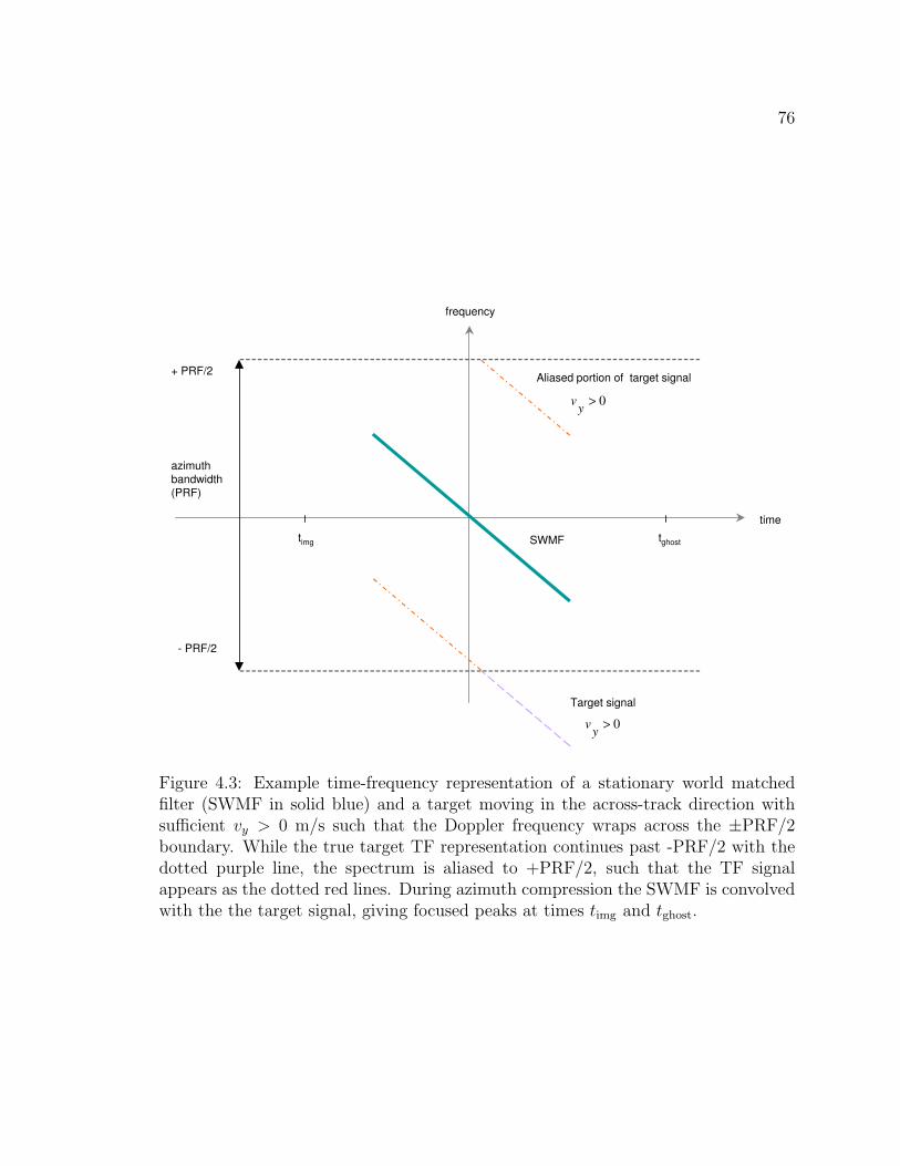
76
time
SWMF
azimuth bandwidth (PRF)
+ PRF/2
- PRF/2
Target signal
Aliased portion of target signal
t img t ghost
0 > y v
0 > y v
frequency
Figure 4.3: Example time-frequency representation of a stationary world matchedfilter (SWMF in solid blue) and a target moving in the across-track direction withsufficient vy > 0 m/s such that the Doppler frequency wraps across the ±PRF/2boundary. While the true target TF representation continues past -PRF/2 with thedotted purple line, the spectrum is aliased to +PRF/2, such that the TF signalappears as the dotted red lines. During azimuth compression the SWMF is convolvedwith the the target signal, giving focused peaks at times timg and tghost.

77
Focusing with along-track velocity vx0
When a target possesses a non-zero along-track velocity component, its azimuth com-
pressed response is characterized by a severe decrease in peak power and by a smear-
ing in azimuth due to azimuthal displacement during the synthetic aperture time.
These effects are illustrated in the bottom frame of Figure 4.1 for a simulated non-
accelerating target with vx = 1 m/s and vy = 0. The decrease in peak power may
again be illustrated in the time-frequency domain (see Figure 4.4). The SWMF has
time
frequency
SWMF
Target signal
azimuth bandwidth (PRF)
synthetic aperture length (T)
+ PRF/2
- PRF/2
0 > x v
Figure 4.4: Example time-frequency representation of a stationary world matchedfilter (SWMF in solid blue of length T seconds) and a target moving in the across-trackdirection with vx > 0 m/s (in dotted red). During azimuth compression the SWMFand target signals are convolved, giving a low power and smeared peak which spreadsacross multiple times in the vicinity of t=0.
a different slope (i.e. Doppler rate) than the moving target’s TF representation. As
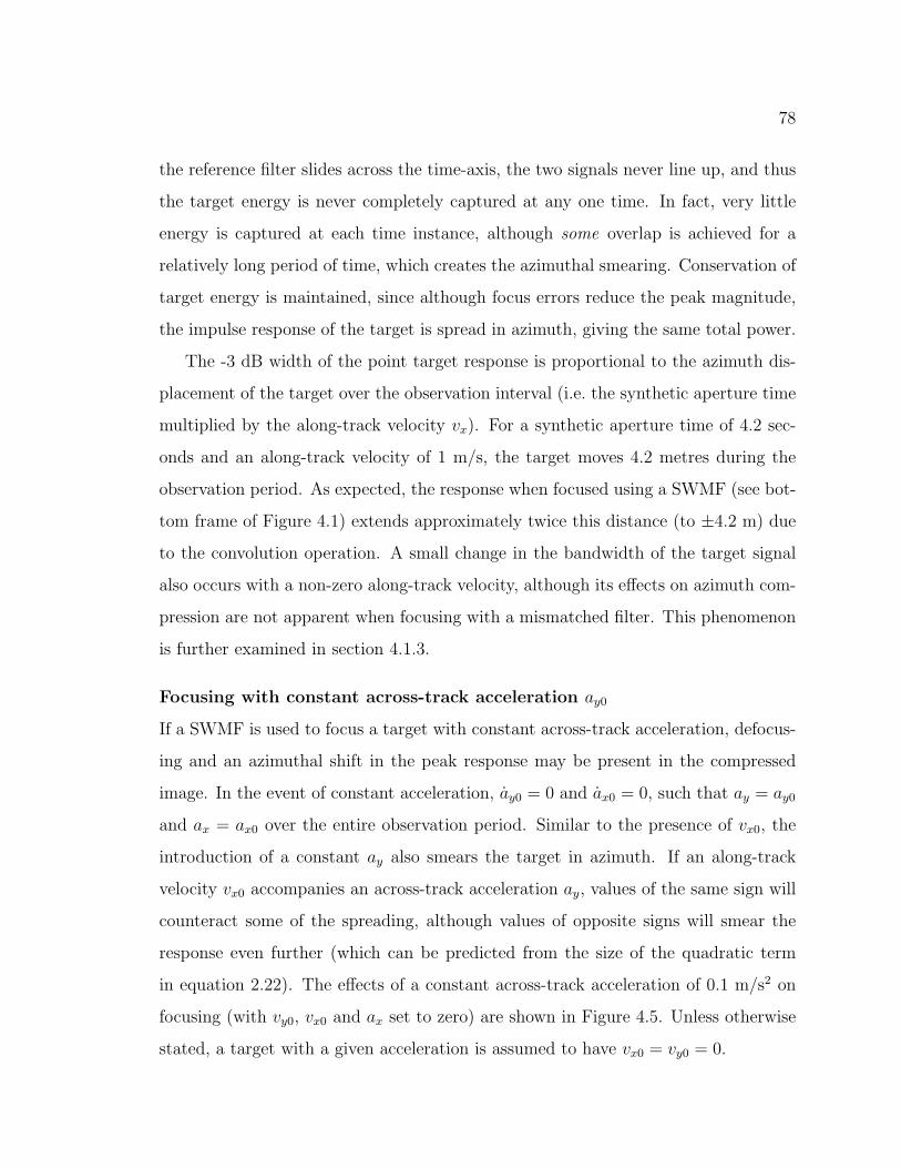
78
the reference filter slides across the time-axis, the two signals never line up, and thus
the target energy is never completely captured at any one time. In fact, very little
energy is captured at each time instance, although some overlap is achieved for a
relatively long period of time, which creates the azimuthal smearing. Conservation of
target energy is maintained, since although focus errors reduce the peak magnitude,
the impulse response of the target is spread in azimuth, giving the same total power.
The -3 dB width of the point target response is proportional to the azimuth dis-
placement of the target over the observation interval (i.e. the synthetic aperture time
multiplied by the along-track velocity vx). For a synthetic aperture time of 4.2 sec-
onds and an along-track velocity of 1 m/s, the target moves 4.2 metres during the
observation period. As expected, the response when focused using a SWMF (see bot-
tom frame of Figure 4.1) extends approximately twice this distance (to ±4.2 m) due
to the convolution operation. A small change in the bandwidth of the target signal
also occurs with a non-zero along-track velocity, although its effects on azimuth com-
pression are not apparent when focusing with a mismatched filter. This phenomenon
is further examined in section 4.1.3.
Focusing with constant across-track acceleration ay0
If a SWMF is used to focus a target with constant across-track acceleration, defocus-
ing and an azimuthal shift in the peak response may be present in the compressed
image. In the event of constant acceleration, ay0 = 0 and ax0 = 0, such that ay = ay0
and ax = ax0 over the entire observation period. Similar to the presence of vx0, the
introduction of a constant ay also smears the target in azimuth. If an along-track
velocity vx0 accompanies an across-track acceleration ay, values of the same sign will
counteract some of the spreading, although values of opposite signs will smear the
response even further (which can be predicted from the size of the quadratic term
in equation 2.22). The effects of a constant across-track acceleration of 0.1 m/s2 on
focusing (with vy0, vx0 and ax set to zero) are shown in Figure 4.5. Unless otherwise
stated, a target with a given acceleration is assumed to have vx0 = vy0 = 0.

79
Figure 4.5: Magnitude response (after azimuth compression) of simulated point tar-gets with constant acceleration focused using a stationary world matched filter versusazimuthal distance. The stationary target response is given as a reference, and an az-imuth of 0 metres is broadside. Top: stationary target. Middle: target with constantacross-track acceleration (ay = 0.1 m/s2, ax = 0) and zero velocity at broadside. Bot-tom: target with constant along-track acceleration (ay = 0, ax = 0.3 m/s2) and zerovelocity at broadside. Note the azimuthal smearing due to ay and the asymmetricsidelobes due to ax.
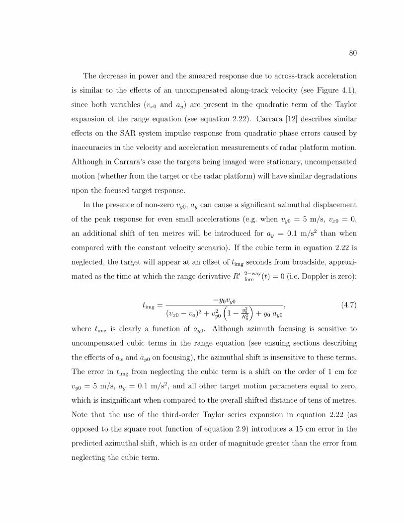
80
The decrease in power and the smeared response due to across-track acceleration
is similar to the effects of an uncompensated along-track velocity (see Figure 4.1),
since both variables (vx0 and ay) are present in the quadratic term of the Taylor
expansion of the range equation (see equation 2.22). Carrara [12] describes similar
effects on the SAR system impulse response from quadratic phase errors caused by
inaccuracies in the velocity and acceleration measurements of radar platform motion.
Although in Carrara’s case the targets being imaged were stationary, uncompensated
motion (whether from the target or the radar platform) will have similar degradations
upon the focused target response.
In the presence of non-zero vy0, ay can cause a significant azimuthal displacement
of the peak response for even small accelerations (e.g. when vy0 = 5 m/s, vx0 = 0,
an additional shift of ten metres will be introduced for ay = 0.1 m/s2 than when
compared with the constant velocity scenario). If the cubic term in equation 2.22 is
neglected, the target will appear at an offset of timg seconds from broadside, approxi-
mated as the time at which the range derivative R′ 2−wayfore (t) = 0 (i.e. Doppler is zero):
timg =−y0vy0
(vx0 − va)2 + v2y0
(1− y2
0
R20
)+ y0 ay0
, (4.7)
where timg is clearly a function of ay0. Although azimuth focusing is sensitive to
uncompensated cubic terms in the range equation (see ensuing sections describing
the effects of ax and ay0 on focusing), the azimuthal shift is insensitive to these terms.
The error in timg from neglecting the cubic term is a shift on the order of 1 cm for
vy0 = 5 m/s, ay = 0.1 m/s2, and all other target motion parameters equal to zero,
which is insignificant when compared to the overall shifted distance of tens of metres.
Note that the use of the third-order Taylor series expansion in equation 2.22 (as
opposed to the square root function of equation 2.9) introduces a 15 cm error in the
predicted azimuthal shift, which is an order of magnitude greater than the error from
neglecting the cubic term.

81
Focusing with constant along-track acceleration ax0
The effects of constant along-track acceleration on focusing are subtle at low mag-
nitudes (e.g. ax = 0.1 m/s2), and thus ax = 0.3 m/s2 is used for emphasis in the
bottom frame of Figure 4.5. Again, to isolate the influence of along-track accelera-
tion, vy0, vx0, and ay are set to zero. Uncompensated along-track acceleration results
in decreased peak power, a slightly wider -3 dB width, and a small azimuthal shift
in the position of the focused peak. However, the principal impact of ax is the cre-
ation of asymmetrical peak sidelobes, with raised sidelobes on one side of the peak
target response and suppressed sidelobes on the other. These findings are consistent
with Carrara’s observations that cubic phase errors cause asymmetric sidelobes in the
system impulse response [12].
Focusing with time-varying across-track acceleration ay(t)
Continuous across-track acceleration The introduction of time-varying across-
track acceleration has additional impact upon the focused SAR response. The -3 dB
coherent integration time (synthetic aperture time) is approximately four seconds for
the simulated airborne scenario previously described, and variation in target acceler-
ation is plausible over this time period (for instance a vehicle accelerating from rest
over the observation period). Such a scenario is illustrated in Figure 4.6, where a
stationary target accelerates to an ay of 0.1 m/s2 over the course of one synthetic
aperture, corresponding to a constant ay0 of 0.024 m/s3.
The target response when focused using a SWMF (see Figure 4.7) has asymmetric
sidelobes due to the uncompensated cubic phase term (to which ay0 contributes in
equation 2.22). Note the severe azimuthal smearing and low peak power despite the
low target velocities and accelerations involved.
Discontinuous across-track acceleration If ay(t) is a continuous function, as in
the above example, then the range expression from equation 2.9 is valid if higher-
order acceleration terms are negligible. However, if ay(t) is discontinuous, then the

82
−2 −1.5 −1 −0.5 0 0.5 1 1.5 20
0.02
0.04
0.06
0.08
0.1
time (s)
a y(t) (m
/s2 )
−2 −1.5 −1 −0.5 0 0.5 1 1.5 20
0.05
0.1
0.15
0.2
time (s)
v y(t) (m
/s)
Figure 4.6: Across-track acceleration ay(t) (with constant ay0) and correspondingacross-track velocity vy(t) for a point target through time, where t=0 corresponds tobroadside. The target’s azimuth response upon compression with a SWMF is givenin Figure 4.7.

83
−20 −15 −10 −5 0 5 10 15 200
0.1
0.2
0.3
0.4
0.5
0.6
0.7
0.8
0.9
1
azimuth (m)
|I 1(t)|
Figure 4.7: Magnitude response (after azimuth compression) of a simulated pointtarget (with constant ay0 and an ay(t) given in Figure 4.6) focused using a stationaryworld matched filter versus azimuthal distance. An azimuth of 0 metres is broadside.Note the low power and severe asymmetric smearing due to ay0.

84
expression in equation 2.9 representing the y position of the target (y = y0 + vy0t +
12ay0t
2 + 16ay0t
3) does not give the correct y away from time t=0. Although in the real
world target range histories will be continuous functions, the radar signal data have
been sampled at the PRF and are thus discrete. If a target is moving at a constant
velocity and then suddenly begins accelerating over a time interval less than the
sampling rate, its acceleration and the time-derivative of acceleration will certainly
be discontinuous.
To expand any function into an nth order Taylor series, it is required that the
function has continuous derivatives of orders one through n [1]. If this condition is
not met, then the range equation must instead be represented as a series of functions
that are piecewise continuous. An example of such an acceleration time-history is
given in the top portion of Figure 4.8, where the target is initially at rest. An
acceleration of 0.1 m/s2 is introduced 0.5 seconds before broadside time, maintained
for one second, then dropped back to zero. The range from the target to the fore
antenna R1(t) consists of three continuous functions: R1−1(t), R1−2(t) and R1−3(t),
such that fore signal s1(t) becomes:
s1(t) = A1(t) exp
(− jk2
(R1−1(t) + R1−2(t) + R1−3(t)
))rect
(t
T
), (4.8)
where
R1−1(t) 6= 0 for − T/2 < t < t1
R1−2(t) 6= 0 for t1 ≤ t ≤ t2
R1−3(t) 6= 0 for t2 < t < T/2,
where t1 is -0.5 seconds and t2 is 0.5 seconds for this scenario. The focused magnitude
response of this target is given in Figure 4.9. The peak response at broadside is
significantly lowered compared to the stationary case, and a secondary peak of similar
magnitude is created approximately five metres off broadside. Additional smaller
peaks are found between the two larger ones, thus smearing the target energy over

85
−2 −1.5 −1 −0.5 0 0.5 1 1.5 2
0
0.02
0.04
0.06
0.08
0.1
time (s)
a y(t) (m
/s2 )
−2 −1.5 −1 −0.5 0 0.5 1 1.5 2−0.02
0
0.02
0.04
0.06
0.08
0.1
time (s)
v y(t) (m
/s)
Figure 4.8: Across-track acceleration ay(t) (a rectangular window centred at broad-side) and corresponding across-track velocity vy(t) for a point target through timewhose azimuth response to a SWMF is given in Figure 4.9.
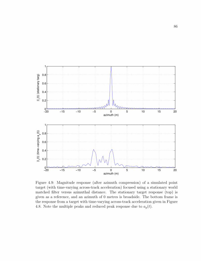
86
−20 −15 −10 −5 0 5 10 15 200
0.2
0.4
0.6
0.8
1
azimuth (m)
|I 1(t)| (
stat
iona
ry ta
rg)
−20 −15 −10 −5 0 5 10 15 200
0.2
0.4
0.6
0.8
1
azimuth (m)
|I 1(t)| (
time−
vary
ing
a y(t))
Figure 4.9: Magnitude response (after azimuth compression) of a simulated pointtarget (with time-varying across-track acceleration) focused using a stationary worldmatched filter versus azimuthal distance. The stationary target response (top) isgiven as a reference, and an azimuth of 0 metres is broadside. The bottom frame isthe response from a target with time-varying across-track acceleration given in Figure4.8. Note the multiple peaks and reduced peak response due to ay(t).

87
many resolution cells. The presence of time-varying across-track acceleration can thus
have a severe effect on target focusing.
The focused (azimuth compressed) target responses to additional across-track ac-
celeration scenarios were also tested. The time-varying acceleration effects can be
seen more clearly by introducing accelerations which are asymmetric about broadside
time. In a second simulation, an across-track acceleration of 0.1 m/s2 is introduced
0.8 seconds after broadside time, maintained for one second, and then once again
dropped to zero. Plots of the time-varying velocity and acceleration, and the focused
target track (when applying a SWMF) are shown in Figure 4.10. These may be com-
pared with the response from a stationary target shown in the top portion of Figure
4.9.
In both acceleration scenarios (from Figures 4.9 and 4.10 (b)), smearing of the
focused responses, decreased peak power, and increased -3 dB widths of the peak
are evident. Spurious responses are introduced to one side of broadside (where the
sidelobe location depends on whether the target is accelerating or decelerating, and
whether acceleration occurs before or after broadside time). If acceleration is asym-
metric about broadside time (as in Figure 4.10), the smearing will appear in one
sidelobe and well-removed from the main target response in azimuth. However, when
the acceleration is symmetric about broadside time (as in Figure 4.8), the acceleration
sidelobes may overlap the mainlobe response. Again, these findings are confirmed by
Carrara who found that cubic phase errors (to which time-varying acceleration con-
tributes) may distort the mainlobe and will raise sidelobes on one side of the impulse
response [12].
A third across-track acceleration configuration was simulated in which a station-
ary target experiences a sudden jump in acceleration of 0.1 m/s2 at broadside time,
after which the acceleration remains constant. Although the acceleration occurs at
broadside time, it continues for the remainder of the observation period (as opposed
to other scenarios in which it is dropped back to zero), and the acceleration side-

88
−2 −1.5 −1 −0.5 0 0.5 1 1.5 2
0
0.02
0.04
0.06
0.08
0.1
time (s)
a y(t) (m
/s2 )
−2 −1.5 −1 −0.5 0 0.5 1 1.5 2
0
0.05
0.1
time (s)
v y(t) (m
/s)
(a) Across-track acceleration ay(t) (a rectan-gular window centred at 1.3 s past broadside)and corresponding across-track velocity vy(t)for a point target through time.
−20 −15 −10 −5 0 5 10 15 200
0.1
0.2
0.3
0.4
0.5
0.6
0.7
0.8
0.9
1
azimuth (m)
|I 1(t)|
(b) Corresponding magnitude re-sponse (after azimuth compression)of a simulated point target (withtime-varying across-track accelera-tion given in the previous figure)focused using a stationary worldmatched filter versus azimuthal dis-tance.
Figure 4.10: Across-track acceleration ay(t) (a rectangular window centred at 1.3s past broadside) for a simulated point target, corresponding across-track velocityvy(t), and its magnitude response (after azimuth compression) when focused using aSWMF. An azimuth of 0 metres is broadside. Note the large sidelobe and reducedpeak response due to ay(t).

89
lobes do not interfere with the mainlobe response. The acceleration and velocity
time-histories, and the azimuth compressed response for this target are shown in Fig-
ures 4.11 and 4.13, respectively. Since the time during which the target experiences
−2 −1.5 −1 −0.5 0 0.5 1 1.5 2
0
0.02
0.04
0.06
0.08
0.1
time (s)
a y(t) (m
/s2 )
−2 −1.5 −1 −0.5 0 0.5 1 1.5 2
0
0.05
0.1
0.15
0.2
time (s)
v y(t) (m
/s)
Figure 4.11: Across-track acceleration ay(t) (a unit step function with height 0.1m/s2) and corresponding across-track velocity vy(t) for a point target through timewhose azimuth response to a SWMF is given in Figure 4.13.
acceleration has been greatly extended, this leads to much wider sidelobes prior to
broadside time than in the previous scenarios. If the target was decelerating instead
of accelerating, the same sidelobes would appear on the opposite side of the peak
response (i.e. after t=0 at an azimuth location location greater than 0 m).
A fourth scenario similar to the third simulation was constructed in which the
acceleration begins 0.5 seconds before broadside and is then ramped up over 0.5 sec-
onds to 0.1 m/s2, after which it remains constant for the remainder of the observation
period. The ramping is done to avoid sudden changes in acceleration (possibly mak-
ing the simulation more realistic), although the time-derivative of acceleration is still
discontinuous at the times acceleration starts and ends, even with this model. Plots

90
of the time-varying velocity and acceleration, and the focused target after correlation
with the SWMF are shown in Figures 4.12 and 4.13. The focused response from the
ramped accelerating target is similar to that from the target with sudden accelera-
tion change, although the acceleration sidelobe in the ramped case has been shifted
slightly further from broadside since the acceleration begins earlier in the observation
interval.
−2 −1.5 −1 −0.5 0 0.5 1 1.5 2
0
0.02
0.04
0.06
0.08
0.1
time (s)
a y(t) (m
/s2 )
−2 −1.5 −1 −0.5 0 0.5 1 1.5 2
0
0.05
0.1
0.15
0.2
time (s)
v y(t) (m
/s)
Figure 4.12: Across-track acceleration ay(t) and corresponding across-track velocityvy(t) for a point target through time whose azimuth response to a SWMF is given inFigure 4.13. The acceleration has been slowly ramped up over 0.5 seconds to simulatemore realistic vehicle situations.
Summarizing, both continuous and discontinuous time-varying across-track ac-
celeration results in asymmetrical sidelobes in the azimuth compressed image after
focusing with a SWMF. Even small changes in ay over the course of the synthetic
aperture will create significant sidelobes. Simulations using similar (e.g. 0.1 m/s2)
changes in along-track acceleration ax had insignificant effects on azimuth focusing,
and thus a separate section of results is not presented.

91
−20 −15 −10 −5 0 5 10 15 200
0.1
0.2
0.3
0.4
0.5
0.6
0.7
0.8
0.9
1
azimuth (m)
|I 1(t)|
discontinuous ay(t)
ramped ay(t)
Figure 4.13: Magnitude response (after azimuth compression) of simulated pointtargets (with time-varying across-track accelerations given in Figures 4.11 and 4.12)focused using a stationary world matched filter versus azimuthal distance. Responsesfrom both discontinuous and ramped accelerations are given, and an azimuth of 0metres is broadside. Note the similar smeared azimuthal response and reduced peakresponse due to ay(t) in both cases.

92
Focusing in a spaceborne geometry
Having examined the influence of target acceleration on focusing for an airborne
scenario, simulations of a spaceborne geometry were conducted. Parameters typical
of the RADARSAT-2 sensor (see Table 3.2) were used in the simulations. As in the
previous spaceborne simulations, the azimuthal beamwidth was set as 0.4◦, although
the PRF was increased to its maximum value of 3800 Hz to increase the level of detail
visible in the focused response. Again, as described in section 3.2.6, the simulations
did not account for earth curvature or rotation effects, but should give an indication
of the consequences of uncompensated target motion on focusing for the space-based
case.
Uncompensated across-track velocity vy0 results in significant shifts off of broad-
side (as observed for the airborne case) for even small velocities (e.g. a shift of -90 m
off broadside is observed for a constant vy = 1 m/s). However, the spaceborne case
is less sensitive to along-track velocity vx0. This is due to the fact that the quadratic
term (vx0 − va)2/(2R0) from the range equation (equation 2.11) is not heavily influ-
enced by vx0 due to the very large va component, such that along-track velocities
upwards of 5 m/s are required before smearing effects become evident. The mag-
nitude responses of a stationary target and moving targets with constant velocity
for the RADARSAT-2 spaceborne geometry are shown in Figure 4.14. The -3 dB
azimuth resolution is on the order of 3.6 m for the stationary target (compared to
0.5 m in the airborne scenario) due to the shortened coherent integration time in the
space-based case of one second (instead of 4.2 s as in the airborne scenario).
Although along-track velocity and across-track acceleration both appear in the
quadratic term of the range equation (equation 2.11), the y0ay0/(2R0) term is of
the same order in both the airborne and spaceborne cases, and thus across-track
acceleration is expected to have a larger impact on spaceborne target focusing than
along-track velocity. Simulations reveal that across-track accelerations on the order
of 0.1 m/s2 or larger are required before smearing is noticeable, where the slightly

93
−10 −5 0 5 100
0.5
1
azimuth (m)
|I 1(t)| (
stat
iona
ry ta
rg)
−100 −95 −90 −85 −800
0.5
1
azimuth (m)
|I 1(t)| (
v x = 0
, vy =
1 m
/s)
−10 −5 0 5 100
0.5
1
azimuth (m)
|I 1(t)| (
v x = 5
m/s
, vy =
0)
Figure 4.14: Magnitude response (after azimuth compression) of simulatednon-accelerating point targets focused using a stationary world matched filter ver-sus azimuthal distance for a spaceborne geometry. The stationary target response isgiven as a reference, and an azimuth of 0 metres is broadside. Top: stationary target.Middle: target with across-track velocity (vy = 1 m/s, vx = 0). Bottom: target withalong-track velocity (vy = 0, vx = 5 m/s). Note the large azimuthal shift due to vy
and the azimuthal smearing due to vx.

94
reduced sensitivity to acceleration compared to the airborne case is due to the coarser
azimuthal resolution. The middle frame of Figure 4.15 shows the severe smearing
resulting from a simulated target with ay=0.2 m/s2.
Along-track acceleration appears in the cubic term of equation 2.11 as the factor
ax0(vx0−va)/(2R0), which is approximately two times smaller in the spaceborne versus
airborne case. Additionally, this factor is multiplied by t3, which is small for |t| < 1,
thus reducing the contribution of the third-order term to the range equation due to
the shortened observation time in the spaceborne scenario. As a consequence, only
extremely large along-track accelerations of 10 m/s2 or higher (which are unrealistic
for the ground vehicles of interest) will have a discernible impact on the focusing of
moving targets. The lower frame of Figure 4.15 depicts the magnitude response from
a simulated target with ax = 10 m/s2, where the small azimuthal shift and raised
sidelobes due to an uncompensated cubic term are visible.
Similarly to ax, time-varying across-track acceleration is not as much of a concern
in the spaceborne case due to the shortened synthetic aperture time of one second for
the RADARSAT-2 scenario. Again, largely unrealistic acceleration rates of change
(e.g. ay0 > 5 m/s3) were required to influence target focusing.
Consequences of a zero-velocity assumption
This section has revealed the severe effects of uncompensated target motion on the
focused magnitude response from a point target for both airborne and spaceborne
geometries. When focused using a SWMF, across-track velocity results in a large
azimuthal displacement from a scatterer’s true position, having ramifications on image
interpretation if it is not known whether the object is moving, or if its direction and
speed are unknown.
Along-track velocity creates severe spreading of the impulse response, such that
targets may be indistinguishable from the background clutter in the azimuth com-
pressed imagery. The airborne scenario has a greater sensitivity to along-track target
motion than the RADARSAT-2 spaceborne case, although there will a noticeable im-

95
Figure 4.15: Magnitude response (after azimuth compression) of simulated pointtargets with constant acceleration focused using a stationary world matched filterversus azimuthal distance for a spaceborne geometry. The stationary target responseis given as a reference, and an azimuth of 0 metres is broadside. Top: stationarytarget. Middle: target with constant across-track acceleration (ay = 0.2 m/s2, ax = 0)and zero velocity at broadside. Bottom: target with constant along-track acceleration(ay = 0, ax = 10 m/s2) and zero velocity at broadside. Note the azimuthal smearingdue to ay and the asymmetric sidelobes due to ax.

96
pact on the compressed imagery using either platform for the range of target velocities
of interest.
Across-track acceleration results in a small azimuthal shift (whose magnitude is
also dependent upon the broadside across-track velocity vy0) and significant smearing
of the target magnitude response. Both the airborne and spaceborne geometries are
sensitive to this parameter, and even small accelerations on the order of 0.1 m/s2
will result in a severely defocused magnitude response. Mismatched reference filters
due to uncompensated vx0 and ay may also influence target detection if detection is
performed in the azimuth compressed domain, since the signal-to-clutter (SCR) ratio
may be lowered to below 0 dB as the target energy is spread across multiple azimuth
cells.
Along-track acceleration and time-varying across-track acceleration will create
asymmetric raised sidelobes which may be mistaken as additional targets in the fo-
cused image. For velocities typical of ground vehicles, these terms pose a potential
problem in the airborne scenario only, since the cubic term of the range equation (in
which these motion parameters appear) is much smaller in the space-based case.
4.1.3 Focusing a moving target with a matched reference filter
The previous section described the effects on focused imagery when applying a SWMF
to a moving target. In those cases, the correlation could not be performed analyt-
ically due to exponential quadratic and cubic terms, and azimuth compression was
performed numerically. However, if these exponential quadratic and cubic terms were
removed by the reference filter, the integration could be completed in closed form.
The following sections investigate the form of the focused target response when a
perfectly matched filter is used and when one matched to the quadratic (but not
linear) term is used. Finally, estimation of the target motion parameters (essential in
defining a properly matched reference filter) is briefly discussed.
Note that if a range compressed signal matrix is focused using a filter matched

97
to the motion of one target, it results in all other signals being mismatched (i.e. de-
focused) in the processed image. Since there are a variety of motions affecting the
different scatterers in a scene, they cannot all be optimally processed simultaneously
[64]. The signal strength of a target refocused under a perfectly matched filter is
expected to increase due to the coherent integration gain. Meanwhile, stationary tar-
gets such as discrete clutter will be blurred in the output of a moving target filter [41].
Thus, the moving target filter suppresses clutter magnitudes and leads to increased
signal-to-clutter ratios (SCRs), which may be a significant advantage in detection and
parameter estimation.
Perfectly matched moving target filter
Although no closed form expression may be derived when correlating a moving target
with a SWMF, one may consider the response of the fore channel data to a filter
r1 matched(t) which is matched to the correct vx0, vy0, ay0, ax0 and ay0:
r1 matched(t) = exp
(− 2jk(R1(t)−R0)
)rect
(t
T
)(4.9)
= exp
(− 2jk
{y0vy0
R0
t +1
2R0
[(vx0 − va)
2 + v2y0
(1− y2
0
R20
)+ y0ay0
]t2
+1
2R0
[vy0ay0
(1− y2
0
R20
)+ ax0(vx0 − va) +
y0 ay0
3
]t3
})rect
(t
T
).
If the matched filter in equation 4.9 is correlated with the signal s1(t) given in
equation 2.12, there is one residual quadratic term∫
exp(Ctτ 2) dτ (where C is a
constant coefficient) that must be integrated. This term exists for non-zero ax0 and
ay0, and results in azimuthal smearing in the compressed SAR response such that it
cannot be neglected. Thus, even a perfectly matched filter will not focus the target
into a well-defined sinc function if there are significant third-order terms in the Taylor
expansion of the range equation.
However, one may consider the scenario in which ax0 and ay0 are zero, such that
the third-order term of the Taylor series expansion of the range equation is neglegibly

98
small. The correlation integral is then a linear function of τ and may be integrated
in closed form. Performing the cross-correlation from equation 4.1 and assuming that
the antenna gain is removed such that the signal amplitude is no longer a function of
time, then the focused moving target image for the fore channel is given by:
I1(t) =A1 (T − |t|)
Texp
(− jk2R1(t)
)exp
(jkαt2
)(4.10)
· sinc
(k(T − |t|) αt
)rect
(t
2T
),
where α =1
R0
[(vx0 − va)
2 + v2y0
(1− y2
0
R20
)+ y0ay0
]. (4.11)
The maximum of I1(t) occurs when the argument of the sinc function is zero, and
thus the peak response of the focused target appears at broadside time t=0 which
coincides with the true broadside position of the scatterer. The first zero crossings of
I1(t) occur when the argument of the sinc function is ±π, i.e. at:
t =±T ∓
√T 2 − 2λ
α
2. (4.12)
Assuming typical airborne geometries, the -3 dB width of the sinc function in equation
4.10 is heavily dependent upon the parameters vx0 and ay0, and to a much lesser
extent on vy0. In section 4.1.1 it was found that a stationary target processed with
a SWMF had a -3 dB width of 0.47 metres. Variations in vx0, ay0 and vy0 (see the
quadratic coefficient in equation 2.11) influence the Doppler rate of change between
the target and the radar platform, resulting in a broadening or narrowing of the
impulse response. If the target is travelling in the opposite direction to the radar
platform (with negative vx0), the Doppler rate increases and the available azimuth
bandwidth will also increase, thus improving azimuth resolution. Conversely, a target
travelling parallel to the radar (with positive vx0) will have a lower Doppler bandwidth
and thus a slightly poorer along-track resolution. If the target is accelerating in the
positive y (across-track) direction (i.e. away from from the radar with ay0 > 0), again
the increased Doppler bandwidth will give finer azimuth resolution, with the opposite

99
occurring for target deceleration. The corresponding impulse response functions of
a focused target for several test scenarios varying vx0 and ay0 are shown in Figure
4.16. Along-track velocities of ±30 m/s worsen/improve the -3 dB width by a factor
−3 −2 −1 0 1 2 30
0.1
0.2
0.3
0.4
0.5
0.6
0.7
0.8
0.9
1
azimuth (m)
|I 1(t)|
stationary targ.v
x0 = 30 m/s
vx0
= −30 m/sa
y0 = 1 m/s2
Figure 4.16: Impulse responses of simulated point targets focused using perfectlymatched filters. An azimuth of 0 metres is broadside. The -3 dB width of thestationary target response is 0.47 m, 0.82 m for vx0 = 30 m/s, 0.26 m for vx0 = −30m/s and 0.30 m for ay0 = 1 m/s2.
of approximately 1.7, and across-track accelerations of ±1 m/s2 improve/worsen the
-3 dB width by a factor of 1.6.
These results are expected based on the azimuthal slow-time resolution predicted
in equation 4.12; positive vx0 and negative ay0 will decrease the value of the square
root term from T (and thus coarsen the resolution) whereas negative vx0 and positive
ay0 will have the reverse effect (improving resolution by allowing the square root term
to approach T ). Since v2y0 (from α in equation 4.11) is expected to be much smaller

100
than y0ay0 and v2a, its effect on resolution is minor compared with that of ay0 and vx0.
Aft Channel We may compute the closed form focused response from the aft signal
data if we again use the matched filter from equation 4.9, retaining the linear and
quadratic terms and assuming ax0 and ay0 are zero such that the cubic term may
be dropped. The reference filter is matched perfectly to the target dynamics, and
upon correlation of signal s2(t) with r1 matched(t), the following compressed image is
obtained:
I2(t) =A2 (T − |t|)
Texp
(− jk[2R1(t) + g(t)]
)exp
(jk[αt + β]t
)(4.13)
· sinc
(k(T − |t|)(αt + β)
)rect
(t
2T
)where
β =α
2
d
va
+d
2R0
(vx0 − va) (4.14)
g(t) =y0vy0
R0
d
va
+ α
(d
va
t +d2
4v2a
)+
d(vx0 − va)
R0
(t +
d
2va
), (4.15)
and α is given in equation 4.11.
The sinc function in the focused aft channel data is similar to that from the
fore channel (see equation 4.10). Despite the added β term in the sinc argument,
the peak response of the aft channel is shifted only a few centimetres from that of
the fore channel and is thus much less than one resolution cell for typical airborne
scenarios (e.g. for vx = 30 m/s, the shift is 9 cm whereas one azimuth resolution cell
is over 80 cm in length, although the azimuth pixel spacing is only 19 cm for the CV
580 system). The shift of the sinc peaks when using RADARSAT-2 parameters is
four orders of magnitude smaller than in the airborne case. These small shifts will
impact the magnitude if the signals are combined (e.g. by computing the DPCA or
ATI signal), although the most significant difference between the fore and aft focused
signals arises in the extra phase terms. Along-track interferometry (see Chapter 6)
makes use of this phase difference for parameter estimation.

101
Moving target filter matched to the quadratic term
Oftentimes, the across-track velocity vy0 of the target is unknown prior to azimuth
compression and thus cannot be included in the reference filter. However, even with-
out compensation of target vy0, the target response may be derived in closed form.
Assuming that the quadratic term in the signal data is known (where the quadratic
coefficient may be estimated using a bank of matched filters, see Chapter 5), and that
ax0 and ay0 are zero, the only uncompensated term in the target signal is the linear
term containing vy0. The focused response of a target in the fore and aft channels
from a reference filter matched to everything but vy0 is:
I1(t) =A1 (T − |t|)
Texp
(− jk2R1(t)
)exp
(jk[
y0vy0
R0
t + αt2]
)(4.16)
· sinc
(k(T − |t|)
[y0vy0
R0
+ αt
])rect
(t
2T
)I2(t) =
A2 (T − |t|)T
exp
(− jk[2R1(t) + g(t)]
)(4.17)
· exp
(jk[
y0vy0
R0
t + αt2 + βt]
)· sinc
(k(T − |t|)
[y0vy0
R0
+ αt + β
])rect
(t
2T
),
where I1(t) and I2(t) are the compressed signals from the fore and aft channels,
respectively, α is given in equation 4.11, β in equation 4.14, and g(t) in equation
4.15.
The peak response of the fore channel I1(t) occurs when the argument of the sinc
function goes to zero at time t = timg from equation 4.7. The focused imaging time
is determined primarily by the across-track velocity vy0 (assuming y0, va, and R0 are
fixed). This shift in the focused peak away from broadside is the azimuthal shift
caused by across-track motion described in section 4.1.2 and well-documented in the
literature (e.g. [17, 20, 35, 41, 62, 80, 90, 93]). As before, the aft channel response
I2(t) is centred at essentially the same location as that of the fore channel.
A reference filter matched to the quadratic range term thus enables one to obtain
a focused image of the target - albeit at a shifted location from broadside - for non-

102
zero vy0. Note that there is no smearing of the impulse response due to a reference
filter unmatched in across-track velocity. However, the finite azimuth bandwidth
of the signal will compromise this focusing, such that a reference filter completely
unmatched in vy0 may still pose some problems. These issues are further described
in Appendix B.1.
Parameter Estimation
A major difficultly in achieving a focused moving target is determining the correct
target velocities and accelerations with which to construct the reference filter. The lit-
erature describing parameter estimation is quite extensive on determining across-track
velocity vy and slightly less so in determining along-track velocity vx. No techniques
are available with which to estimate accelerations since the problem becomes under-
determined with a greater number of unknowns than equations when only two SAR
channels of data are available. In most instances, it is assumed that the targets are
moving at a constant velocity, whether or not this is actually the case. A summary
of parameter estimation methods used in GMTI was presented in section 2.3.2.
Rather than estimate the target motion parameters themselves, one can compress
the signal data with a bank of reference filters initialized with various quadratic
and/or linear coefficients. The compressed image from the filter returning the highest
magnitude when correlated with the target signal is then retained for subsequent
analysis. It may be assumed that this method was applied to initialize the reference
filters described in section 4.1.3.
4.2 Experimental Results
After examining the theoretical response of accelerating targets to various matched
filters, azimuth compression was carried out on experimental data from the CV 580
airborne system. A description of the data set and its preprocessing is described in
Appendix A. It is assumed that the moving targets have already been detected and

103
have had their tracks extracted through azimuth time as described in section 3.3.
It is verified that stationary point targets can be successfully focused before turning
our attention to the results of using a SWMF and filters matched to various motion
parameters to compress moving targets in azimuth.
4.2.1 Focusing a stationary target
To ensure that the focusing algorithm being applied is correct, the responses from
stationary corner reflectors in experimental data were examined. A correct focusing
algorithm is critical in examining the effectiveness of matched filtering the moving
target track data.
The time domain correlation operation from equation 4.1 is more efficiently imple-
mented in the Fourier domain, where the convolution becomes a multiplication. The
Fourier transform of the signal data and the time-reversed complex conjugate of the
reference signal are taken using two FFTs. The FFTs are then multiplied together,
and the inverse FFT is performed to transform the data back into the time domain.
A weighting function (such as a cosine-shaped Hanning window) is applied to the ref-
erence function to reduce the sidelobes of the point spread function. When focusing
stationary targets, the length of the reference function was set as the length of the
-3 dB width at the range bin of interest. For focusing moving targets, the reference
function length was chosen to be the length of the detected target track.
Stationary corner reflectors are a reasonable approximation of a point target which
may be used to verify the compression algorithm. Unfortunately, in the Petawawa
2000 data all corner reflectors at the designated calibration site were set mere metres
from the ARCs (Active Radar Calibrators). Consequently, in the imagery one cannot
distinguish the two responses. This was not a problem in a second data set collected
in the Ottawa area in 2001 with the same airborne system. Focusing the calibration
site data, it was found that the corner reflectors’ responses were two-dimensional sinc
functions, with -3 dB widths of approximately 0.95 metres in azimuth and 5.6 metres

104
in range. These values are very close to the resolution limits of the system (quoted
as 0.85 metres in azimuth and 5.7 metres in range [46]), and thus the compression
algorithm is functioning as expected. Figure 4.17 displays one example of a focused
stationary corner reflector from the Ottawa 2001 data set. Note the high peak power
and narrow mainlobe of the focused image.
4.2.2 Focusing a moving target with a SWMF
From section 4.1, we expect that moving targets focused using a SWMF may suffer
from azimuthal displacement, a loss of peak power, smearing of the impulse response,
and asymmetric sidelobes, where the particular image degradations will depend upon
their motion parameters.
In order to isolate the target signal and suppress clutter, the DPCA signal was
computed for each target track by subtracting the two channels. As described in
section 4.1.3, the azimuth compressed fore and aft signals are nearly coincident sinc
functions with a phase difference which is a function of the target motion parameters.
If compressed using a filter matched to at least the quadratic coefficient, the DPCA
signal is a sinc-like response with high peak power and low sidelobes, and is free from
clutter interference (although mathematically it is not an exact sinc).
The aircraft headings and target GPS data indicate that each controlled mover
had both along-track and across-track motion components. Because each target has
non-zero along-track velocity vx0 (and possibly non-zero ay) every target was smeared
upon azimuth compression with a SWMF. The focused image after DPCA for one
pass of the Convoy target is given in Figure 4.18. The wide mainlobe and low peak
power indicate non-zero vx0 and/or ay0, and the asymmetric sidelobes point to possible
ax0 and/or ay0 acceleration components. Time-frequency analysis is used to obtain a
focused image of this target in section 7.3.4.

105
−10 −8 −6 −4 −2 0 2 4 6 8 10
0.2
0.4
0.6
0.8
1
1.2
azimuth (m)
Mag
nitu
de
(a) Magnitude response of corner reflector.
−10 −8 −6 −4 −2 0 2 4 6 8 10−55
−50
−45
−40
−35
−30
−25
−20
−15
−10
−5
0
azimuth (m)
Mag
nitu
de (d
B)
(b) Magnitude response of corner reflector in decibels,normalized to 0 dB.
Figure 4.17: Magnitude response after azimuth compression of a stationary cornerreflector from the Ottawa 2001 data set. Note the narrow mainlobe and high peakpower. The -3 dB width is approximately 1.1 m.

106
−15 −10 −5 0 5 10 150
0.01
0.02
0.03
0.04
0.05
0.06
0.07
0.08
azimuth (m)
|DP
CA
|
Figure 4.18: Magnitude response (after clutter suppression using DPCA) for a movingtarget (l1p9 Convoy) focused using a SWMF. Note the low peak power, wide main-lobe, and asymmetric sidelobes which indicate possible acceleration components.

107
4.2.3 Focusing a moving target with a matched reference filter
Next it was attempted to focus each moving target using a reference filter matched to
the quadratic and linear components of the received signal. As described in section
4.1.3, the creation of a matched reference filter requires knowledge of the motion
parameter vector. Using a bank of matched filters (which is described more thoroughly
in Chapter 5) the quadratic coefficient of the fore channel signal s1(t) is approximated.
Using the ATI phase (described in detail in Chapter 6), the across-track velocity vy0
is estimated and used to initialize the linear coefficient of the reference filter. The
third-order coefficient is assumed to be negligible, which is a reasonable assumption
if there is no acceleration.
However, even after matched filtering with these estimated parameters, most tar-
gets remain unfocused, some showing virtually no improvement at all in focusing.
Two examples of targets focused using a SWMF and a matched filter initialized with
the best estimates of the linear and quadratic signal coefficients are shown in Figures
4.19 and 4.20. A filter matched to the moving target’s phase history is abbreviated
as MTMF (moving target matched filter). Note that an azimuth of 0 m is arbitrarily
set at the location of each peak response such that the width of the mainlobe can be
read directly off each graph. In actuality, the position of the focused target will shift
significantly in azimuth upon compensation of the linear (vy0) term, as was described
in section 4.1. Figure 4.19 shows significant improvement in focusing with the use
of a MTMF over a SWMF, such that the mainlobe has narrowed, and there is a
higher peak power, although there are still significant sidelobes. The target depicted
in Figure 4.20 shows no improvement in focusing with the use of a MTMF, perhaps
indicating the presence of a significant uncompensated cubic term or indicating that
there is an error in the quadratic coefficient used in the matched filter. Both az-
imuth compressed targets focused using a MTMF are not ideal sinc functions, and
thus there is some uncompensated platform-target motion. The residual sidelobes
from both target images are typical of the entire data set. A different method is

108
−40 −30 −20 −10 0 10 20 30 400
0.005
0.01
0.015
0.02
0.025
0.03
azimuth (m)
|DP
CA
|
(a) Focused image using a stationary worldmatched filter (SWMF).
−40 −30 −20 −10 0 10 20 30 400
0.05
0.1
0.15
0.2
0.25
0.3
0.35
0.4
azimuth (m)
|DP
CA
|
(b) Focused image using a moving targetmatched filter (MTMF).
Figure 4.19: DPCA magnitude after azimuth compression of one pass of the Convoytarget using a stationary world matched filter and a moving target matched filter.Note the change in scale of the y-axes between the two plots. The MTMF is ini-tialized with estimates of the linear and quadratic signal coefficients, although allcubic and higher-order coefficients remain uncompensated. Note the large increasein peak power and narrower mainlobe when filtering with a MTMF, although theresponse is still not an ideal sinc function, indicating the presence of uncompensatedplatform-target motion such as an uncompensated cubic term.

109
−40 −30 −20 −10 0 10 20 30 400
0.2
0.4
0.6
0.8
1
1.2
1.4
1.6
azimuth (m)
|DP
CA
|
(a) Focused image using a stationary worldmatched filter (SWMF).
−40 −30 −20 −10 0 10 20 30 400
0.2
0.4
0.6
0.8
1
1.2
1.4
1.6
azimuth (m)
|DP
CA
|
(b) Focused image using a moving targetmatched filter (MTMF).
Figure 4.20: DPCA magnitude after azimuth compression of one pass of the Juliettarget using a SWMF and a MTMF. The MTMF is initialized with estimates of thelinear and quadratic signal coefficients, although all cubic and higher-order coeffi-cients remain uncompensated. There is little improvement in focusing between theSWMF and MTMF. Both possess significant sidelobes indicative of uncompensatedradar-target motion.

110
thus required to obtain a focused image of the moving targets. This issue is further
examined using time-frequency analysis in Chapter 7.
Having derived the azimuth compressed fore and aft channel expressions in this
chapter, we can examine the effects of acceleration on banks of matched filters (for
estimation of vx0) and on ATI phase (for estimation of vy0) in the next two chapters.

111
Chapter 5
Estimation of along-track velocity vx0
After detection of a moving target, it is often desirable to determine its velocity in the
along- and across-track directions. This information is useful for monitoring ground
vehicles, repositioning them to their true azimuth broadside location on the image,
and extrapolating a target’s future position.
The objective of this chapter is to describe the impact of acceleration on estimating
the along-track velocity vx0, and the repercussions of a zero-acceleration assumption.
The effects of acceleration on along- and across-track velocity estimation are very
different, which is why the treatment of each velocity component is given in separate
chapters.
Along-track velocity estimation is accomplished using a bank of matched filters
to focus the target data, and then searching for the filter giving the maximum mag-
nitude response. This algorithm is described, followed by an analysis of the effect of
each motion parameter (velocities and accelerations) on the resulting vx0 estimate.
Simulations of the filter-bank responses to stationary, constant velocity, and acceler-
ating targets are carried out for both airborne and spaceborne geometries. As in the
previous chapter, theory and simulations are combined due to difficulties in analyt-
ically maximizing the cross-correlation expression involved in azimuth compression.
Finally, the matched filter-bank algorithm is applied to experimental data to estimate
the along-track velocity of each target. These velocity estimates are compared to GPS
velocities, and the similarities and discrepancies between the values are discussed.
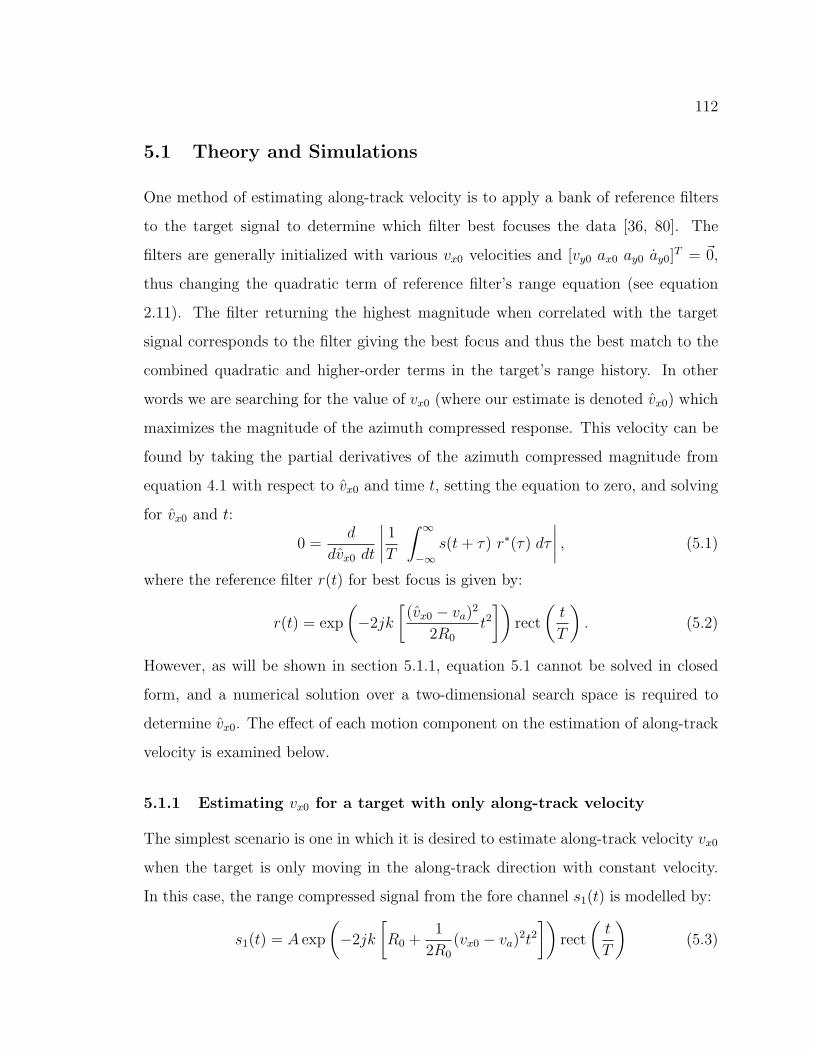
112
5.1 Theory and Simulations
One method of estimating along-track velocity is to apply a bank of reference filters
to the target signal to determine which filter best focuses the data [36, 80]. The
filters are generally initialized with various vx0 velocities and [vy0 ax0 ay0 ay0]T = ~0,
thus changing the quadratic term of reference filter’s range equation (see equation
2.11). The filter returning the highest magnitude when correlated with the target
signal corresponds to the filter giving the best focus and thus the best match to the
combined quadratic and higher-order terms in the target’s range history. In other
words we are searching for the value of vx0 (where our estimate is denoted vx0) which
maximizes the magnitude of the azimuth compressed response. This velocity can be
found by taking the partial derivatives of the azimuth compressed magnitude from
equation 4.1 with respect to vx0 and time t, setting the equation to zero, and solving
for vx0 and t:
0 =d
dvx0 dt
∣∣∣∣ 1T∫ ∞
−∞s(t + τ) r∗(τ) dτ
∣∣∣∣ , (5.1)
where the reference filter r(t) for best focus is given by:
r(t) = exp
(−2jk
[(vx0 − va)
2
2R0
t2])
rect
(t
T
). (5.2)
However, as will be shown in section 5.1.1, equation 5.1 cannot be solved in closed
form, and a numerical solution over a two-dimensional search space is required to
determine vx0. The effect of each motion component on the estimation of along-track
velocity is examined below.
5.1.1 Estimating vx0 for a target with only along-track velocity
The simplest scenario is one in which it is desired to estimate along-track velocity vx0
when the target is only moving in the along-track direction with constant velocity.
In this case, the range compressed signal from the fore channel s1(t) is modelled by:
s1(t) = A exp
(−2jk
[R0 +
1
2R0
(vx0 − va)2t2])
rect
(t
T
)(5.3)

113
Substituting equations 5.2 and 5.3 into the maximization from equation 5.1 we have
the following:
0 =d
dvx0 dt
∣∣∣∣∣ 1T∫ ∞
−∞A exp
(−2jk
[R0 +
1
2R0
(vx0 − va)2(t + τ)2
])(5.4)
· exp
(2jk
[(vx0 − va)
2
2R0
τ 2
])rect
(t + τ
T
)rect
( τ
T
)dτ
∣∣∣∣∣.Terms not a function of τ may be pulled out of the integration and the exponential
terms may be regrouped as:
0 =d
dvx0dt
∣∣∣∣∣AT exp
(−2jk
[R0 +
1
2R0
(vx0 − va)2t2])
·∫ ∞
−∞exp
(−2jk
[(vx0 − va)
2
2R0
(2tτ) +1
2R0
[(vx0 − va)
2 − (vx0 − va)2]τ 2
])· rect
(t + τ
T
)rect
( τ
T
)dτ
∣∣∣∣∣. (5.5)
Analytically equation 5.5 cannot be solved in closed form because of the integration
of the exponential quadratic term τ 2. Instead, a two-dimensional search over the
synthetic aperture time −T/2 ≤ t ≤ T/2 s and over the along-track velocity range of
interest (e.g. −30 ≤ vx0 ≤ 30 m/s) is required to determine the parameters returning
the maximum magnitude in the azimuth compressed response. This search can be
performed using a simple algorithm to create a bank of reference filters initialized
with various vx0 values. The signal data is convolved with each reference filter in
turn, and the output is saved to a matrix, which is then scanned to find the location
of the maximum magnitude value. Oftentimes, the DPCA signal is compressed using
the filter-bank rather than only the fore or aft channel in order to avoid obtaining
maxima due to clutter from discrete targets.
Along-track velocity was estimated using this filter-bank and search method for
simulated signal data of a point target travelling in the along-track direction. The
DPCA signal was not used since it is zero for vy0 = 0, as was described in Chapter
3, and here we wish to observe the effects of a vx0 velocity component only. From

114
equation 5.5, it is seen that if vx0 = vx0, then the quadratic τ 2 term in the inte-
gration disappears and the azimuth compressed signal will be the modulated sinc
function given in equation 4.10. This sinc function has high peak power (there is no
azimuthal smearing), and it is thus expected that this reference filter will give the
largest magnitude response in the compressed imagery at broadside time t = 0.
Simulations were used to verify the unbiasedness of the vx0 estimate for a target
moving only with constant vx0 and all other motion parameters set to zero. An
airborne geometry typical of the CV 580 system (with radar and geometry parameters
given in Table 3.1) was simulated. A point target was given an along-track velocity vx0
of 10 m/s, with all other velocity components set to zero. A filter-bank of 300 reference
filters was created with azimuth velocities ranging from -30 to 30 m/s. Along-track
velocities were evenly spaced along this interval every 0.2 m/s. Figure 5.1 shows
an enlarged image of the resulting ‘filter-bank map’ after azimuth compression with
each reference filter. Each row of the filter-bank map corresponds to the output after
compression using one reference filter. There is a clear peak at a vx0 = 10 m/s (the
true target velocity) and time t = 0 (the true broadside position of the target), and
thus the estimate is unbiased.
5.1.2 Estimating vx0 in the presence of vy0
Next, the estimation of vx0 using the filter-bank method is investigated in the presence
of non-zero across-track velocity vy0. Again, the analytical expression maximizing the
magnitude response cannot be solved in closed form. However, we can use observa-
tions from section 4.1.3 to predict the output of the matched filter-bank method for
non-zero vx0 and vy0. When compressing a signal with a reference filter matched to
the quadratic component of the target signal but not the linear component (as in
section 4.1.3), it was found that the focused response is still a sinc function although
it is shifted in azimuth to a position related to the across-track velocity vy0. Thus, we
expect that a target with non-zero vy0 will give a well-focused peak in the filter-bank

115
azimuth (m)
v x0 (m
/s)
−20 −15 −10 −5 0 5 10 15 205
6
7
8
9
10
11
12
13
14
15
0.1
0.2
0.3
0.4
0.5
0.6
0.7
0.8
0.9
Figure 5.1: Magnitude responses of a simulated point target with constant vx0 = 10m/s (and all other motion parameters set to zero) after compression with a bank ofreference filters initialized with various vx0 velocities. An azimuth of 0 m is broadside.Note that vx0 (estimated from the location of peak power) matches the true targetvelocity of 10 m/s.

116
map, although it will be shifted away from broadside.
One problem with the proposed matched filter-bank algorithm is that it assumes
the quadratic coefficient in the range equation is due solely to contributions from
along-track target-platform motion (i.e. from vx0 and va). However, as seen in
equation 2.11, the second-order component of the range equation also contains a
v2y0(1−y2
0/R20) term which will bias the estimation of vx0, especially in the presence of
large vy0 velocities. This bias can be determined by equating the assumed quadratic
coefficient (from the reference filter of equation 5.2) with the true quadratic coefficient
(from equation 2.11):
1
2R0
[(vx0 − va)
2]
=1
2R0
[(vx0 − va)
2 + v2y0
(1− y2
0
R20
)]. (5.6)
Solving for vx0:
vx0 = va −
√(vx0 − va)2 + v2
y0
(1− y2
0
R20
), (5.7)
where it has been assumed that |vx0| � |va| such that only one solution is retained.
The bias in the velocity estimate is (vx0 − vx0).
According to equation 5.7, the largest biases in vx0 will occur for large positive
vx0 and large vy0 of either sign. For example, for a moving point target with vx0 =
vy0 = 30 m/s and zero acceleration, equation 5.7 predicts a bias of 2.7 m/s for the
CV 580 airborne scenario. A target travelling completely in the across-track direction
(i.e. vx0 = 0) with large vy0 = 30 m/s will create a bias of 2.1 m/s in the estimate of vx0
(from equation 5.7). The output filter-bank map for this situation from a simulated
point target after DPCA is shown in Figure 5.2. As expected there is an azimuthal
shift in the location of the peak response away from broadside due to the presence
of across-track velocity vy0. The azimuthal shift is not 1.5 km (as predicted by the
timg of equation 4.7 multiplied by va) due to the finite synthetic aperture footprint;
the focused response must fall within the synthetic aperture such that the response
wraps around to give the -88 m displacement observed in Figure 5.2. As predicted
by equation 5.7, the vx0 estimated from the filter-bank approach is biased by 2.1 m/s

117
azimuth (m)
v x0 (m
/s)
−105 −100 −95 −90 −85 −80 −75 −70−6
−5
−4
−3
−2
−1
0
1
2
0.2
0.4
0.6
0.8
1
1.2
1.4
Figure 5.2: DPCA magnitude responses of a simulated point target with vy0 = 30m/s (and all other motion parameters set to zero) after compression with a bank ofreference filters initialized with various vx0 velocities. An azimuth of 0 m is broadside.Note that vx0 (estimated from the location of peak power) is biased by 2.1 m/s, sincethe true along-track velocity is zero.
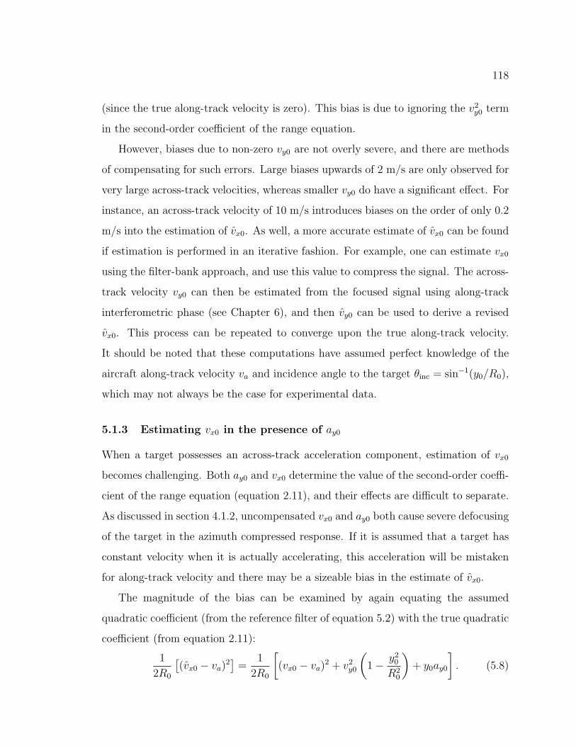
118
(since the true along-track velocity is zero). This bias is due to ignoring the v2y0 term
in the second-order coefficient of the range equation.
However, biases due to non-zero vy0 are not overly severe, and there are methods
of compensating for such errors. Large biases upwards of 2 m/s are only observed for
very large across-track velocities, whereas smaller vy0 do have a significant effect. For
instance, an across-track velocity of 10 m/s introduces biases on the order of only 0.2
m/s into the estimation of vx0. As well, a more accurate estimate of vx0 can be found
if estimation is performed in an iterative fashion. For example, one can estimate vx0
using the filter-bank approach, and use this value to compress the signal. The across-
track velocity vy0 can then be estimated from the focused signal using along-track
interferometric phase (see Chapter 6), and then vy0 can be used to derive a revised
vx0. This process can be repeated to converge upon the true along-track velocity.
It should be noted that these computations have assumed perfect knowledge of the
aircraft along-track velocity va and incidence angle to the target θinc = sin−1(y0/R0),
which may not always be the case for experimental data.
5.1.3 Estimating vx0 in the presence of ay0
When a target possesses an across-track acceleration component, estimation of vx0
becomes challenging. Both ay0 and vx0 determine the value of the second-order coeffi-
cient of the range equation (equation 2.11), and their effects are difficult to separate.
As discussed in section 4.1.2, uncompensated vx0 and ay0 both cause severe defocusing
of the target in the azimuth compressed response. If it is assumed that a target has
constant velocity when it is actually accelerating, this acceleration will be mistaken
for along-track velocity and there may be a sizeable bias in the estimate of vx0.
The magnitude of the bias can be examined by again equating the assumed
quadratic coefficient (from the reference filter of equation 5.2) with the true quadratic
coefficient (from equation 2.11):
1
2R0
[(vx0 − va)
2]
=1
2R0
[(vx0 − va)
2 + v2y0
(1− y2
0
R20
)+ y0ay0
]. (5.8)

119
Solving for vx0 we obtain:
vx0 = va −
√(vx0 − va)2 + v2
y0
(1− y2
0
R20
)+ y0ay0, (5.9)
where the bias is again (vx0 − vx0).
Assuming vy0 = 0 in order to isolate the effects of ay0, and assuming an airborne
geometry typical of the CV 580 system, equation 5.9 predicts a bias of -23.5 m/s for
an acceleration of ay0 = 1 m/s2 and vx0 = 0. Even a slight acceleration of ay0 = 0.1
m/s2 introduces a bias of -2.5 m/s, as shown in the filter-bank map of Figure 5.3.
The DPCA response is not shown because it is negligible when vy0 = 0, as in this
scenario.
azimuth (m)
v x0 (m
/s)
−5 −4 −3 −2 −1 0 1 2 3 4 5−4.5
−4
−3.5
−3
−2.5
−2
−1.5
−1
−0.5
0.1
0.2
0.3
0.4
0.5
0.6
0.7
0.8
0.9
Figure 5.3: Magnitude responses of a simulated point target with ay0 = 0.1 m/s2 (andall other motion parameters set to zero) after compression with a bank of referencefilters initialized with various vx0. An azimuth of 0 m is broadside. Note that vx0
(estimated from the location of peak power) is biased by -2.5 m/s, since the truealong-track velocity is zero.
Across-track acceleration can thus introduce significant biases when estimating
vx0 if it assumed that targets travel at a constant velocity. However, even if one

120
acknowledges the possibility of across-track acceleration, ay0 will be indistinguishable
from vx0; they are both contained in the quadratic coefficient of the range equation
and they cannot be estimated independently in the absence of a priori data (such as
from inertial systems onboard the target) or additional SAR channels.
Across-track acceleration combined with non-zero across-track velocity (as is gen-
erally the case in realistic moving target scenarios) introduces a small cubic component
into the target range history according to equation 2.11. From the range equation it
is theoretically possible to solve for ay0 (assuming ax0 = ay0 = 0) by implementing
a three-dimensional match filter-bank algorithm to determine the third-order coeffi-
cient. However, for the range of target velocities and accelerations of interest, the
contribution of ay0 to this component is virtually negligible; it is ax0 and ay0 which
are dominant in determining the cubic component.
5.1.4 Estimating vx0 in the presence of ax0
In the presence of an along-track acceleration component, the target signal has a
significant cubic term as predicted in the range equation (see equation 2.11). When
the filter-bank method is applied to the data, it is attempted to match a quadratic
reference filter to a cubic signal. As described in section 4.1.2, this results in an
uncompensated third-order component whose impacts on the azimuth compressed
response include:
• a smearing of the target energy across multiple vx0 velocities in the filter-bank
and multiple cells in azimuth, which severely decreases peak power
• the creation of two vx0 peaks (instead of one) (where, for instance, the peaks
are shifted from zero in the stationary case to ±0.3 m/s for an ax0 = 0.5 m/s2
and all other motion parameters set to zero)
• a slight shift in the azimuth focused position (the two peaks focus at an az-
imuth 0.4 m away from broadside for an ax0 = 0.5 m/s2 and all other motion

121
parameters set to zero)
Some of these effects may be seen in a comparison between the filter-bank mag-
nitude image of a stationary target, and a target with ax0 = 0.5 m/s2 (with all other
motion paramters set to zero) in Figure 5.4. The most striking effect is the decrease
azimuth (m)
v x0 (m
/s)
Stationary Target
−5 0 5−2
−1.5
−1
−0.5
0
0.5
1
1.5
2
0.1
0.2
0.3
0.4
0.5
0.6
0.7
0.8
0.9
azimuth (m)
v x0 (m
/s)
Target with ax0
= 0.5 m/s2
−5 0 5−2
−1.5
−1
−0.5
0
0.5
1
1.5
2
0.1
0.2
0.3
0.4
0.5
0.6
0.7
0.8
0.9
Figure 5.4: Magnitude responses of a simulated point target with ax0 = 0.5 m/s2 (andall other motion parameters set to zero) after compression with a bank of referencefilters initialized with varying vx0. An azimuth of 0 m is broadside. Note the smearingof target energy across multiple vx0 velocities in the accelerating case, and the smallbias in estimated vx0 on the order of 0.3 m/s.
in peak power of the target responses (evident from the common color bars between
the accelerating and stationary cases); the full target energy is never captured by one
vx0 filter since none of the reference filters represents the true phase history of the
target through time. This uncompensated cubic term creates asymmetric sidelobes
(visible in Figure 5.4 as fringes extending in the positive azimuth direction) as was
observed in section 4.1.2. Also apparent in Figure 5.4 is the smearing of target en-
ergy across multiple vx0 filters. This effect is perhaps most easily examined in the

122
time-frequency domain (which was introduced in section 2.4). As mentioned in sec-
tion 2.4.2, time-frequency analysis is useful for examining a target’s instantaneous
Doppler frequency, which may be found by taking the derivative of the target phase
history and dividing by 2π to obtain units of Hz. Recall that the target phase history
is given by the argument of the exponential term in equations 2.24 and 2.25 for the
fore and aft channels, respectively, yielding a quadratic expression for instantaneous
frequency. However, if there is no target acceleration, frequency varies linearly with
time and reduces to the following equation:
f(t) =−2
λ
[y0vy0
R0
+1
2R0
[(vx0 − va)
2 + v2y0
(1− y2
0
R20
)]t
], (5.10)
where f(t) represents the instantaneous frequency.
The time-frequency history for a non-accelerating target can thus be represented
by a line, whose slope is determined principally by vx0 and whose y-intercept is de-
termined by vy0. The line has finite start and end points determined by the synthetic
aperture length. Matched filtering correlates this time-frequency line with a reference
signal. This reference is generally chosen as another line; a stationary world matched
filter (SWMF) is a line with a y-intercept of zero, and a slope of −v2a/(λR0).
When attempting to focus a target, a bank of matched filters is initialized with
various vx0 velocities (i.e. lines of various slopes in the TF domain). The filter return-
ing the highest magnitude when correlated with the target signal corresponds to the
chosen estimate of vx0. However, for a target with non-zero ax0, the time-frequency
history is a quadratic function (as opposed to a linear one), and thus there is no
one best vx0 filter (or TF line) to capture the entire target energy. An exaggerated
diagram of this effect is illustrated in Figure 5.5.
In reality the time-frequency history will appear only slightly non-linear since the
quadratic TF coefficient is much smaller than the linear coefficient. However, the
effect is significant enough to impact the matched filtering process. In Figure 5.4,
two peaks are observed in the filter-bank of the accelerating target. This could be
due to two lines of different slopes (as pictured in Figure 5.5) giving relatively large

123
Figure 5.5: Example time-frequency history for a target accelerating in the along-trackdirection (solid black line). The nonlinear component of the TF history has beengreatly exaggerated for demonstration purposes. For reference, the time-frequencyhistory for a stationary target is provided (dashed blue line). The two best-fit lineswhich capture the most target energy (and hence might give two peaks in the fil-ter-bank magnitude map as in Figure 5.4) are shown in red.

124
magnitude responses compared to the other matched filters. If these lines do not
have y-intercepts of 0, then the target will not be focused exactly at broadside (i.e. at
t = 0, or an azimuth x = 0). It can be seen in Figure 5.4 that the peaks are slightly
offset from broadside position by approximately 0.4 metres, although this shift is
negligible when compared to the shift induced by an uncompensated across-track
velocity component.
Uncompensated ax0 will introduce small biases into the estimation of vx0 velocity
(on the order of 1 m/s for ax0 = 1 m/s2). However the most severe effect is a decrease
in peak power which may make it difficult to find the location of peak power and thus
to estimate vx0, especially in the presence of residual clutter and noise.
5.1.5 Estimating vx0 in the presence of ay0
Since both ax0 and ay0 appear in the cubic coefficient of the range equation (see
equation 2.11), it is expected that the effects of time-varying across-track acceleration
on vx0 estimation would be very similar to the impact of along-track acceleration
ax0. This was confirmed in simulations of the CV 580 airborne geometry. Figure
5.6 displays the filter-bank magnitude map for a point target with ay0 = 0.04 m/s3
and all other motion parameters set to zero. There is a bias in the estimate of vx0
which is on the order of 0.6 m/s for the simulated scenario. Again, perhaps the most
problematic effect is the decrease in peak power and severe smearing, which makes it
difficult to identify the true peaks in the filter-bank magnitude map for noisy signal
data. This in turn can lead to errors in the estimated along-track velocity.
5.1.6 Estimating vx0 in a spaceborne geometry
In addition to airborne geometries, estimation of along-track velocity was conducted
for a simulated spaceborne RADARSAT-2 scenario (see parameters in Table 3.2) for
targets possessing various motion components. The influences of target motion on vx0
estimation as observed in the airborne scenarios are very similar to the spaceborne

125
azimuth (m)
v x0 (m
/s)
Stationary Target
−5 0 5−2
−1.5
−1
−0.5
0
0.5
1
1.5
2
0.1
0.2
0.3
0.4
0.5
0.6
0.7
0.8
0.9
azimuth (m)
v x0 (m
/s)
Target with aydot
= 0.04 m/s2
−5 0 5−2
−1.5
−1
−0.5
0
0.5
1
1.5
2
0.1
0.2
0.3
0.4
0.5
0.6
0.7
0.8
0.9
Figure 5.6: Magnitude responses of a simulated point target with ay0 = 0.04 m/s3
(and all other motion parameters set to zero) after compression with a bank of ref-erence filters initialized with various vx0 velocities. An azimuth of 0 m is broadside.Note the similarities to uncompensated along-track acceleration ax0 in Figure 5.4,including a small bias in the estimate of vx0 on the order of 0.6 m/s .

126
case, although the sensitivity of the estimation to various motion parameters may
change due to differences in the scale of the radar-target geometry.
In the presence of an along-track velocity component only, as in the airborne
case, there is no bias in estimating vx0. However, due to the large platform velocity
(i.e. large va), the sensitivity of the quadratic term to small changes in vx0 decreases,
and thus the precise location of the peak response is more difficult to determine in
the space-based case, which will decrease the accuracy with which one may estimate
vx0. Figure 5.7 is the filter-bank magnitude for a target with vx0 = 10 m/s and all
other motion parameters set to zero observed in a spaceborne radar-target geometry.
Although well-localized in azimuth, note the large peak power for vx0 velocities in the
vicinity of the true vx0 = 10 m/s value.
azimuth (m)
v x0 (m
/s)
−30 −20 −10 0 10 20 30−10
−5
0
5
10
15
20
0.1
0.2
0.3
0.4
0.5
0.6
0.7
0.8
0.9
Figure 5.7: Magnitude responses of a simulated point target for a spaceborne geome-try with vx0 = 10 m/s (and all other motion parameters set to zero) after compressionwith a bank of reference filters initialized with various vx0 velocities. An azimuth of0 m is broadside. Note that vx0 matches the true target velocity of 10 m/s, althoughthe location of peak power is not as well defined as it is in the airborne case.

127
In the spaceborne case, targets with large across-track velocities on the order
of 30 m/s have no discernible effect on the estimation of vx0. In this geometry, the
v2y0(1−y2
0/R20) term in the second-order component of the range equation is sufficiently
small compared to the value of (vx0−va)2 (also in the quadratic component) that the
bias in vx0 is negligible; no iteration or two-step process is required (as was suggested
for the airborne case in section 5.1.2) for an accurate estimate of vx0.
However, the spaceborne case is even more sensitive to biases in vx0 caused
by across-track accelerations than the airborne situation. For instance, an across-
acceleration of ay0 = 0.1 m/s2 introduces a bias of -4.5 m/s in vx0 for the spaceborne
case compared to a bias of -2.5 m/s in the airborne scenario. Along-track accelera-
tion and time-varying across-track acceleration on the other hand, do not noticeably
affect vx0 estimation. There are no apparent asymmetric sidelobes and no discernible
decrease in peak power in the filter-bank magnitude map for |ax0| ≤1 m/s2 and
|ay0| ≤ 0.1m/s3, and a bias of only 0.1 m/s was observed in vx0 for an ax0 = 1 m/s2.
5.2 Experimental Results
To test along-track velocity estimation in experimental data, the filter-bank method
was applied to each of the twenty-two target tracks extracted from the Petawawa
2000 data. Appendix A includes a description of this data set, and section 3.3 details
how the targets were detected and their tracks extracted. A filter-bank of 2000
matched filters with along-track velocities ranging from -30 to 30 m/s (spaced every
0.03 m/s) were used to focus the data. A more sophisticated algorithm may be used
to iterate this operation using progressively denser (i.e. narrowly-spaced) filter-banks
in a smaller velocity range to converge upon the peak response, although only a simple
filter-bank was applied in this instance.
The range compressed fore and aft target tracks were subtracted and then con-
volved with each matched filter to compute the azimuth compressed DPCA signals.
DPCA was used to suppress clutter, thus preventing any clutter from discrete targets

128
(e.g. buildings) from biasing the vx0 estimation. All targets had non-zero across-track
velocity vy0 not equal to a blind velocity, and thus all targets had non-zero DPCA
magnitude. The location of the peak power response in the DPCA filter-bank map
was used to find the filter most closely matched to the true along-track velocity vx0.
The along-track velocities estimated using the filter-bank method for each target
and their velocities as measured using GPS are presented in Appendix A.3. The
procedure to convert GPS velocity into along- and across-track velocity components,
and the expected accuracy in the GPS measurements (approximately 0.5 m/s) are
also detailed in Appendix A.3. Taking the absolute value of the differences between
the GPS velocities and the estimated target velocities, a mean error of 2.9 m/s was
found in vx0 as estimated from the SAR data with a standard deviation of 2.6 m/s. A
number of targets had significant biases in their along-track velocity estimates when
compared to the GPS values, with a maximum bias of 9.3 m/s. These large biases may
indicate the presence of possible along- and across-track acceleration components.
An example of a biased vx0 estimation from one pass of the Convoy target is shown
in Figure 5.8. There is a clear peak response in the filter-bank magnitude map at
a vx0 of 11.5 m/s. However, the GPS velocity is only 5.7 m/s, pointing to a likely
acceleration bias due to ay0 as described in section 5.1.3.
In addition to biases in vx0, the smearing effects and asymmetric sidelobes char-
acteristic of an uncompensated cubic term are also visible in the experimental data.
This suggests that one can predict the existence of a cubic term by examining the
filter-bank magnitude map for the characteristic smearing patterns described in sec-
tions 5.1.4 and 5.1.5. Figure 5.9 shows the filter-bank map from one pass of the
Juliet target in which along-track acceleration ax0 and/or time-varying across-track
acceleration ay0 may be causing the smearing and sidelobe effects as were observed
in simulations. There may also be higher-order target motion components, improper
motion compensation of the platform velocity, incorrect estimates of va, y0/R0 and
other parameters, or residual clutter, which may be having additional impact upon

129
azimuth time (s)
v x0 (m
/s)
3.4 3.45 3.5 3.55 3.6 3.65 3.7 3.75 3.82
4
6
8
10
12
14
16
18
20
0
0.5
1
1.5
2
2.5
3
Figure 5.8: DPCA filter-bank magnitude map from one pass of the Convoy target (line1, pass 5). The peak response occurs at vx0=11.5 m/s, whereas the GPS velocity is5.7 m/s, indicating a severe bias in the vx0 estimate which may be due to the presenceof across-track acceleration ay0.

130
the filter-bank map.
azimuth time (s)
v x0 (m
/s)
−2 −1.95 −1.9 −1.85 −1.8 −1.75 −1.7−8
−6
−4
−2
0
2
4
6
8
10
12
14
0
0.5
1
1.5
2
2.5
3
3.5
Figure 5.9: DPCA filter-bank magnitude map from one pass of the Juliet target (line2, pass 2). In addition to a bias in the vx0 estimate, this target displays asymmetricsidelobes to the left-hand side of the peak response and smearing of the target energycharacteristic of an uncompensated cubic component in the focusing operation.
As well, oftentimes, the target energy in the filter-bank magnitude maps is smeared
across multiple vx0 velocities, making it difficult to determine if the correct peak is
being selected by the algorithm. Figure 5.10 displays the filter-bank map for one pass
of Juliet whose peak response is in excellent agreement with the GPS data (within
0.24 m/s). However, despite the accuracy of the estimate, one can see extensive
smearing on the right-hand side, again suggesting an uncompensated cubic term.
Again, higher-order motion components as well as incomplete clutter suppression
may be causing some of the smearing and local maxima effects visible elsewhere in
the image.
Unfortunately, as described in section 3.3.2, it is difficult to determine the target’s
true acceleration since GPS data were only collected every two seconds. Extremely
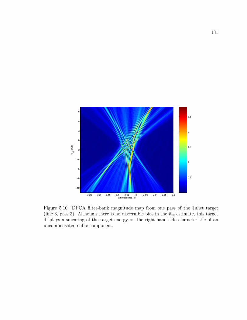
131
azimuth time (s)
v x0 (m
/s)
−3.25 −3.2 −3.15 −3.1 −3.05 −3 −2.95 −2.9 −2.85 −2.8
−10
−8
−6
−4
−2
0
2
4
6
0.5
1
1.5
2
2.5
Figure 5.10: DPCA filter-bank magnitude map from one pass of the Juliet target(line 3, pass 3). Although there is no discernible bias in the vx0 estimate, this targetdisplays a smearing of the target energy on the right-hand side characteristic of anuncompensated cubic component.

132
accurate estimates of acceleration would be needed in any case, since simulations
have shown that one must be concerned with even slight accelerations on the order
of 0.1 m/s2 or less. Future experimental trials could equip controlled movers with
high-accuracy GPS systems functioning at a higher sampling rate and inertial systems
with gyroscopes in order to determine a target’s acceleration time-history.
Summarizing, acceleration (both along- and across-track components) may have
a severe effect on estimation of along-track velocity. This was demonstrated using
theory, simulations, and experimental data. Across-track acceleration ay0 severely
biases the vx0 estimate if it is assumed that targets are travelling at a constant velocity.
If acceleration is acknolwedged as an additional unknown, then there are insufficient
degrees of freedom to solve for all parameters. This issue is further addressed in
Chapter 7. Along-track acceleration ax0 and time-varying across-track acceleration
ay0 also effect vx0 estimation by smearing the target energy across multiple cells in
the filter-bank map and introducing a slight bias in the location of the peak response.
Having described the effects of acceleration on along-track velocity estimation, we
examine its influence on estimating the across-track velocity component in the next
chapter.

133
Chapter 6
Estimation of across-track velocity vy0
Across-track velocity is a fundamental parameter of interest for GMTI applications.
This chapter examines the estimation of across-track velocity using along-track in-
terferometric (ATI) phase, and the impact of acceleration upon this phase. As in
previous chapters, the theory of ATI is reviewed, followed by vy0 estimation using
simulated point targets with various motion components, and ending with examples
from experimental data. The across-track velocities of controlled movers from the
experimental data are estimated using the ATI phase and are compared with GPS
velocities.
6.1 Theory
The along-track interferometric phase computed from two channels of SAR data may
be used to determine the across-track velocity of a target. The history of ATI was
outlined in section 2.3.2 and the basic ATI equation was given in equation 2.27, in
which the fore channel is multiplied by the complex conjugate of the registered aft
channel. The phase is then the argument of the ATI signal, where in the noise-free
case a stationary target should theoretically have zero phase (since fore and registered
aft channels are identical) and a moving target will possess an ATI phase related to
its motion components. The ATI method was chosen to estimate across-track velocity
because of its sensitivity to vy0 compared to other techniques (such as those described
in the latter portions of section 2.3.2). However, ATI phase suffers from a number of
ambiguities which must be resolved prior to velocity estimation. These are outlined
in Appendix B.1.
Along-track interferometric phase is generally computed in the azimuth com-

134
pressed domain for improved signal-to-clutter ratios (see Appendix B.2 for further
explanation). Using the expressions derived for the azimuth compressed signal re-
turns from the fore and aft channels (equations 4.16 and 4.17 from section 4.1.3),
where the reference filter has been matched to the quadratic term of the range equa-
tion only, we can determine a closed form expression for the ATI signal. Applying
equation 2.27 (the ATI equation), and assuming that along-track acceleration ax0 and
across-track acceleration rate ay0 are zero, we have:
ATI(t) = I1(t) I∗2 (t)
=A1 (T − |t|)
Tsinc
(k(T − |t|)
[y0vy0
R0
+ αt
])(6.1)
· A2 (T − |t|)T
sinc
(k(T − |t|)
[y0vy0
R0
+ αt + β
])exp
(jk[g(t)− βt]
).
Substituting equations 4.14 and 4.15 for β and g(t), respectively, and dropping the
negligible d2/v2a term, the ATI phase is given as:
∠ATI(t) =ky0dvy0
R0va
+kd
2R0
t
(vx0 − va) +
[(vx0 − va)
2 + v2y0
(1− y2
0
R20
)+ y0ay0
]va
.
(6.2)
Evaluated at its focused location t = timg from equation 4.7, the ATI phase becomes:
∠ATI(timg) =kdy0vy0
2R0
1
va
− (vx0 − va)
(vx0 − va)2 + v2y0
(1− y2
0
R20
)+ y0ay0
. (6.3)
Note that equation 6.3 is the ATI phase only for a target focused using a reference
filter matched in the quadratic term. If the reference filter contains a non-zero vy0
(and thus a non-zero linear coefficient), then the image focusing time timg will change,
and the ATI phase may be computed using equation 6.2.
6.2 Simulations
Equations 6.2 and 6.3 are verified using simulations for various vx0, vy0 and ay0. The
SAR signals are determined using equation 2.9 to compute the fore channel range

135
history, and equations 2.15 and 2.19 to compute the aft channel range history, which
make use of the far-field approximation only. Additional simulations using non-zero
along-track acceleration ax0 and across-track acceleration rate ay0 are also conducted.
The influence of these parameters on the ATI phase and on the estimation of across-
track velocity is described below. The estimated across-track velocity is denoted vy0.
6.2.1 Variation in ATI with vy0
ATI phase is extremely sensitive to across-track target velocity vy0 since it appears
in the numerator of equation 6.3. This sensitivity may be exploited to derive pre-
cise estimates of the across-track velocity component. However, for vy0 = 0 m/s or
the blind-velocities discussed in Appendix B.1 (corresponding to across-track target
displacements a multiple of λ/2), the ATI phase vanishes and no information for
parameter estimation can be extracted from the ATI phase alone. Polar plots of
the ATI signal at time t = timg for a target with unambiguous across-track speeds
varying from -2.5 to 10 m/s (and all other motion parameters set to zero) are given
in Figure 6.1. Since the ATI magnitude is determined by the multiplication of two
relatively narrow sinc functions (see equation 6.1), the focused image location can be
determined after ATI as the point at which the ATI magnitude is maximum. This
technique may be made more robust using a keyhole filter (as described in Appendix
B.2) to remove interfering clutter with strong amplitudes yet small phases lying close
to the positive real axis.
In the plots of Figure 6.1, one can see distinctly non-zero ATI phase for even small
across-track velocities (e.g. a vy0 of 2.5 m/s gives an ATI phase of approximately
44◦). As well, note that a target with negative across-track velocity has the same
ATI phase as a target with positive vy0 of the same magnitude, except that the
phase has opposite sign. A stationary target has zero ATI phase but has maximum
magnitude, since the reference and target signal functions have complete spectral
overlap. As across-track velocity increases, the spectral overlap decreases, reducing

136
0.2
0.4
0.6
0.8
1
30
210
60
240
90
270
120
300
150
330
180 0
(a) ATI for vy0 = 0 m/s
0.0002
0.0004
0.0006
0.0008
30
210
60
240
90
270
120
300
150
330
180 0
(b) ATI for vy0 = 10 m/s
0.2
0.4
0.6
30
210
60
240
90
270
120
300
150
330
180 0
(c) ATI for vy0 = 2.5 m/s
0.2
0.4
0.6
30
210
60
240
90
270
120
300
150
330
180 0
(d) ATI for vy0 = −2.5 m/s
Figure 6.1: ATI signal for varying across-track velocities vy0 (with zero acceleration).Phase is given in degrees as an angle measured from the positive real axis, andmagnitude as a distance from the origin. Note the sensitivity of the phase to non-zerovy0 and the variation in ATI magnitudes for non-zero vy0.
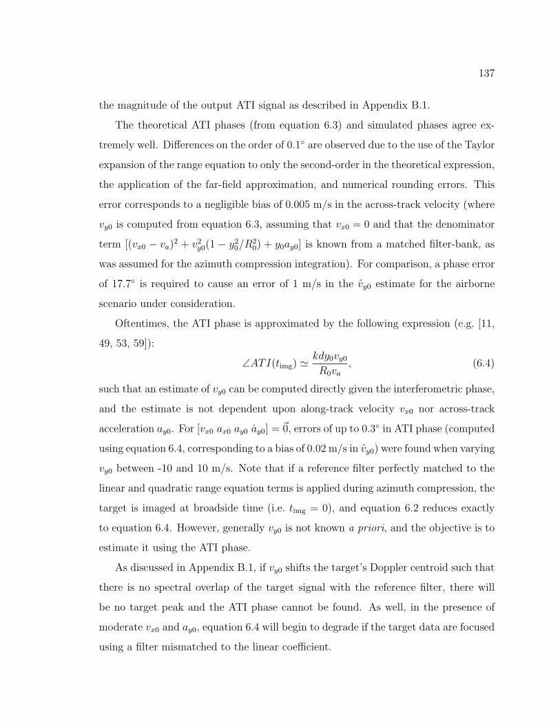
137
the magnitude of the output ATI signal as described in Appendix B.1.
The theoretical ATI phases (from equation 6.3) and simulated phases agree ex-
tremely well. Differences on the order of 0.1◦ are observed due to the use of the Taylor
expansion of the range equation to only the second-order in the theoretical expression,
the application of the far-field approximation, and numerical rounding errors. This
error corresponds to a negligible bias of 0.005 m/s in the across-track velocity (where
vy0 is computed from equation 6.3, assuming that vx0 = 0 and that the denominator
term [(vx0 − va)2 + v2
y0(1 − y20/R
20) + y0ay0] is known from a matched filter-bank, as
was assumed for the azimuth compression integration). For comparison, a phase error
of 17.7◦ is required to cause an error of 1 m/s in the vy0 estimate for the airborne
scenario under consideration.
Oftentimes, the ATI phase is approximated by the following expression (e.g. [11,
49, 53, 59]):
∠ATI(timg) 'kdy0vy0
R0va
, (6.4)
such that an estimate of vy0 can be computed directly given the interferometric phase,
and the estimate is not dependent upon along-track velocity vx0 nor across-track
acceleration ay0. For [vx0 ax0 ay0 ay0] = ~0, errors of up to 0.3◦ in ATI phase (computed
using equation 6.4, corresponding to a bias of 0.02 m/s in vy0) were found when varying
vy0 between -10 and 10 m/s. Note that if a reference filter perfectly matched to the
linear and quadratic range equation terms is applied during azimuth compression, the
target is imaged at broadside time (i.e. timg = 0), and equation 6.2 reduces exactly
to equation 6.4. However, generally vy0 is not known a priori, and the objective is to
estimate it using the ATI phase.
As discussed in Appendix B.1, if vy0 shifts the target’s Doppler centroid such that
there is no spectral overlap of the target signal with the reference filter, there will
be no target peak and the ATI phase cannot be found. As well, in the presence of
moderate vx0 and ay0, equation 6.4 will begin to degrade if the target data are focused
using a filter mismatched to the linear coefficient.

138
6.2.2 Variation in ATI with vx0
As can be seen from equation 6.3, vx0 will influence the ATI phase. The amount it
will shift the ATI phase is dependent both upon the value of vx0 and the across-track
velocity vy0. Examining the theoretical expression for the ATI phase in equation 6.3,
the bias caused by ignoring the vx0 dependence increases indefinitely with increasing
vx0 and vy0. However, this equation does not take into account wrapping of the
spectrum due to a finite azimuth bandwidth. The focused image location timg used to
derive equation 6.3 can only fall between −T and T (twice the original signal length
due to the convolution operation), and thus the error in ATI phase due to ignoring
the vx0 component will not increase indefinitely.
Examining the differences between the simulated ATI phase and that determined
from equation 6.4 for only those target signals with some spectral overlap with the
reference signal, it was found that the maximum bias for −30 ≤ vx0 ≤ 30 m/s and
−30 ≤ vy0 ≤ 30 m/s (scanned in steps of 1 m/s) is 21.7 degrees or 1.2 m/s occurring
at vx0 = −30 m/s and vy0 = ±16 m/s . Figure 6.2 shows some biases between
the vy0-only ATI phase computation and its actual value for a target with vx0 = −30
m/s. These values were computed by taking the simulated ATI phase at its maximum
amplitude, and differencing it from the ATI phase computed from equation 6.4.
If a reference filter closely matched in vy0 (within one m/s) is used to focus the
target data (in addition to being matched in the quadratic term), variation in the ATI
phase with vx0 will bias the vy0 estimate by a maximum of 0.16 m/s, which may or
may not be a concern depending on the required accuracy of the application. When
a reference filter perfectly matched to vy0 is applied in compression, the bias in vy0 is
negligible (for any vx0), and is due only to use of the far-field approximation and the
Taylor series expansion of the range equation.
In the above examples it has been assumed that the quadratic term in the refer-
ence filter has been matched to the quadratic coefficient of the target range history
such that comparisons to the theoretical expression could be made. If this quadratic
139
0.2
0.4
0.6
0.8
1
30
210
60
240
90
270
120
300
150
330
180 0
ATI(timg
)ATI v
y0 only
(a) ATI for vx0 = −30 m/s, vy0 = 0 m/s
0.05
0.1
0.15
30
210
60
240
90
270
120
300
150
330
180 0
ATI(timg
)ATI v
y0 only
(b) ATI for vx0 = −30 m/s, vy0 = 10 m/s
0.2
0.4
0.6
0.8
30
210
60
240
90
270
120
300
150
330
180 0
ATI(timg
)ATI v
y0 only
(c) ATI for vx0 = −30 m/s, vy0 = 2.5 m/s
0.2
0.4
0.6
0.8
30
210
60
240
90
270
120
300
150
330
180 0
ATI(timg
)ATI v
y0 only
(d) ATI for vx0 = −30 m/s, vy0 = −2.5m/s
Figure 6.2: ATI signal for varying across-track velocities vy0 (with zero acceleration)and constant vx0 = −30 m/s (in solid red) compared with the expected ATI phasewhen the vx0 dependence is neglected (in dotted blue). Phase is given in degrees asan angle measured from the positive real axis, and magnitude as a distance from theorigin.

140
term is unmatched then the target will be defocused in both the fore and aft chan-
nels, decreasing the SCR such that the ATI phase will be subject to increased clutter
contamination as described in section B.2. In addition, the smearing of the target
response (as described in section 4.1.2) due to an unmatched quadratic term creates
peaks away from broadside time, such that the peak ATI magnitude is not at broad-
side when vy0 = 0, and the ATI phase at this peak magnitude will give an incorrect
estimate of vy0. This is illustrated in Figure 6.3, where Figure 6.3(a) shows the coinci-
dent fore and aft responses for a point target with vx0 = 10 m/s, vy0 = 0, compressed
using a SWMF, and Figure 6.3(b) shows the target’s ATI phase (for all times, not
just timg). The peak magnitudes occur away from broadside with an ATI phase of
±5.7◦, biasing the computation of vy0 by 0.3 m/s.
6.2.3 Variation in ATI with ay0
Similar to vx0, non-zero ay0 will effect the ATI phase (see the denominator of the
second term in equation 6.3). Because ay0 is multiplied by y0, even small accelerations
such as 0.1 m/s2 will have a noticeable impact upon the phase. For example, for
vx0 = 0 m/s, vy0 = 10 m/s and ay0 = 0.1 m/s2, the ATI phase shifts 3.8 degrees,
creating an error of 0.2 m/s if equation 6.4 is used to compute vy0. This shift may be
lessened or increased in the presence of an along-track velocity depending the signs
of the motion parameters as described in section 4.1.2; vx0 and ay0 of the same sign
will reduce the overall shift, whereas values of opposite signs will increase the shift
in ATI phase. When more severe accelerations (but still plausible) of ±1 m/s2 are
introduced, shifts of up to 36.6◦ (or biases of 2.1 m/s in vy0) are present. Combined
with shifts resulting from vx0 velocity, neglecting the contributions of ay0 to the ATI
phase can give erroneous estimates of vy0. Examples of the effect of ay0 on ATI phase
are shown in Figure 6.4.

141
−0.6 −0.4 −0.2 0 0.2 0.4 0.60
0.01
0.02
0.03
0.04
0.05
0.06
0.07
0.08
0.09
time (s)
Mag
nitu
de
foreaft
(a) Fore and aft target responses(with nearly perfect overlap) com-pressed using a stationary referencefilter.
0.002
0.004
0.006
0.008
0.01
30
210
60
240
90
270
120
300
150
330
180 0
(b) ATI signal of the target (in red)with ATI signal at broadside timegiven in blue.
Figure 6.3: Compressed target response from a SWMF and ATI signal for a pointtarget with vx0 = 10 m/s and all other motion parameters equal to zero. Phase isgiven in degrees as an angle measured from the positive real axis, and magnitudeas a distance from the origin. Note the spread in the ATI phase and note that themaximum channel responses and ATI magnitudes occur at times other than broadsidetime t = 0.

142
0.2
0.4
0.6
0.8
1
30
210
60
240
90
270
120
300
150
330
180 0
ATI(timg
)ATI v
y0 only
(a) ATI for ay0 = 1 m/s2, vy0 = 0 m/s
0.02
0.04
0.06
0.08
0.1
30
210
60
240
90
270
120
300
150
330
180 0
ATI(timg
)ATI v
y0 only
(b) ATI for ay0 = 1 m/s2, vy0 = 10 m/s
0.2
0.4
0.6
0.8
30
210
60
240
90
270
120
300
150
330
180 0
ATI(timg
)ATI v
y0 only
(c) ATI for ay0 = 1 m/s2, vy0 = 2.5 m/s
0.2
0.4
0.6
0.8
30
210
60
240
90
270
120
300
150
330
180 0
ATI(timg
)ATI v
y0 only
(d) ATI for ay0 = 1 m/s2, vy0 = −2.5m/s
Figure 6.4: ATI signal for varying across-track broadside velocities vy0 and constantacross-track acceleration ay0 = 1 m/s2 (in solid red) compared with the expectedATI phase when the ay0 dependence is neglected (in dotted blue). Phase is given indegrees as an angle measured from the positive real axis, and magnitude as a distancefrom the origin.

143
6.2.4 Variation in ATI with ax0 and ay0
Analytically, the ATI phase of a target with non-zero ax0 and/or ay0 components
cannot be computed in closed form. However, we may examine the errors in using
equation 6.4 to estimate vy0 in the presence of along-track acceleration and/or time-
varying across-track acceleration using simulations.
Compared to vx0 and ay0, ax0 and ay0 have a relatively small impact on ATI phase.
For ax0 varied from −1 to 1 m/s2 (scanned in steps of 0.1 m/s2), and vy0 varied from
-30 to 30 m/s (scanned in steps of 1 m/s), the maximum deviation from equation 6.4
was 2.4◦, translating to a bias in vy0 of 0.14 m/s. Similarly, varying ay0 over ±0.1
m/s3 gave a maximum deviation of 4.6◦ or a bias of 0.26 m/s in vy0. Thus, for the
parameter ranges examined, the effects of ax0 and ay0 on ATI phase are nearly an
order of magnitude lower than the influence of vx0 and ay0.
6.2.5 Variation in ATI phase for spaceborne scenarios
The previous sections have presented simulations of the ATI signal based exclusively
on the CV 580 system parameters. The CV 580 airborne system has a comparatively
large azimuth oversampling factor (' 2.8) compared to certain configurations of the
proposed RADARSAT-2 system. The main RADARSAT-2 parameters influencing
ATI phase computations are given in Table 3.2, where both the azimuthal beamwidth
and the PRF are programmable by the operator.
If the azimuth beamwidth is chosen as 0.4◦ and the PRF as 2000 Hz (mid-range
values), and if we are observing a target with an incidence angle of 40◦ from the
satellite, the azimuth oversampling factor will be only 1.1, such that nearly complete
spectral overlap is present between the reference filter and target signal for any target
motion. In this case, the azimuth compression will capture nearly all the target energy
into one peak (due to the large amount of overlap) and the ATI phase will depend
only upon vy0. One disadvantage of the lower overlap factor is that there is little data
uncontaminated by clutter, whereas with a large PRF and a small beamwidth, all

144
signal data with Doppler frequencies outside of the clutter limits and within ±fPRF/2
are free from main-beam clutter (although some sidelobe clutter may remain).
If the azimuth beamwidth is reduced to its minimum of 0.21◦ and the PRF is
increased to its maximum of 3800 Hz, the oversampling factor becomes 3.9, and
thus complete loss of spectral overlap is possible, giving erroneous ATI phase and vy0
estimates. However, for the ground moving target velocities in which we are interested
(−30 ≤ vx0 ≤ 30 m/s and −30 ≤ vy0 ≤ 30 m/s), the maximum bias is only 0.33◦ (or
0.07 m/s). Similarly, ay0 varied in between ±1 m/s2 introduces a maximum bias of
0.83◦ in the ATI phase from equation 6.4 (or 0.13 m/s in vy0). These biases are very
small compared to the expected standard deviation of the ATI phase in the spaceborne
case of 3.2 m/s (derived in section B.2). Because the spaceborne platform moves with
along-track velocity several hundred times faster than the vehicular velocities being
observed, even high target vx0 does not significantly change the Doppler rate (or
slope of the target signal in the TF domain) and its contribution to the ATI phase
in equation 6.3 is small. The denominator of equation 6.3 contains an ay0 term,
but again its contribution is small compared to v2a. As well, even high vy0 does not
significantly shift the Doppler centroid with respect to the total bandwidth, such
that the ±fPRF/2 wrapping will not occur for velocities of interest (at this reduced
azimuth beamwidth and high PRF), and significant spectral overlap will always occur
for velocities of interest. Thus, one need not be concerned with the influence of
vx0, small accelerations (|ax0, ay0| ≤ 1 m/s2), or small across-track acceleration rates
(|ay0| ≤ 0.1 m/s3) on the ATI phase in the RADARSAT-2 scenario.
6.2.6 ATI simulation summary
Along-track interferometric phase has been presented as one metric for estimating the
across-track velocity of a target. However, because ATI uses phase measurements, this
method is subject to ambiguities in its estimates due to directional-ambiguities from
π wraps of the ATI phase and due to sampling limitations in azimuth. The relation
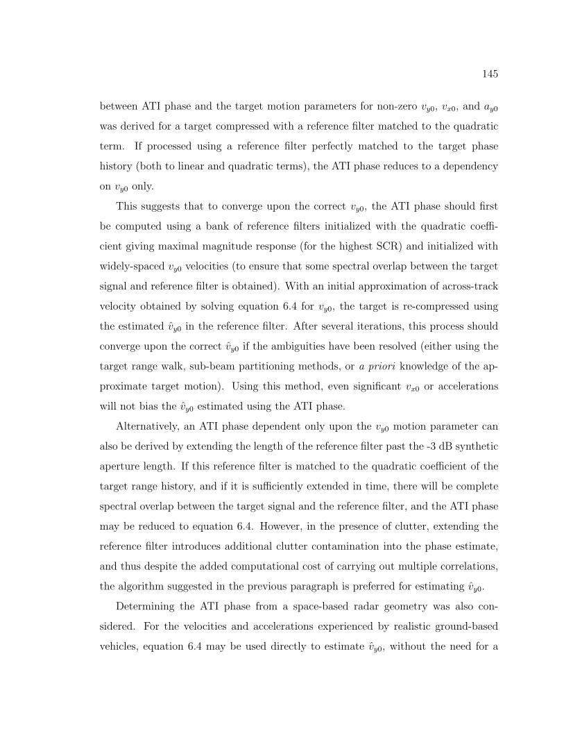
145
between ATI phase and the target motion parameters for non-zero vy0, vx0, and ay0
was derived for a target compressed with a reference filter matched to the quadratic
term. If processed using a reference filter perfectly matched to the target phase
history (both to linear and quadratic terms), the ATI phase reduces to a dependency
on vy0 only.
This suggests that to converge upon the correct vy0, the ATI phase should first
be computed using a bank of reference filters initialized with the quadratic coeffi-
cient giving maximal magnitude response (for the highest SCR) and initialized with
widely-spaced vy0 velocities (to ensure that some spectral overlap between the target
signal and reference filter is obtained). With an initial approximation of across-track
velocity obtained by solving equation 6.4 for vy0, the target is re-compressed using
the estimated vy0 in the reference filter. After several iterations, this process should
converge upon the correct vy0 if the ambiguities have been resolved (either using the
target range walk, sub-beam partitioning methods, or a priori knowledge of the ap-
proximate target motion). Using this method, even significant vx0 or accelerations
will not bias the vy0 estimated using the ATI phase.
Alternatively, an ATI phase dependent only upon the vy0 motion parameter can
also be derived by extending the length of the reference filter past the -3 dB synthetic
aperture length. If this reference filter is matched to the quadratic coefficient of the
target range history, and if it is sufficiently extended in time, there will be complete
spectral overlap between the target signal and the reference filter, and the ATI phase
may be reduced to equation 6.4. However, in the presence of clutter, extending the
reference filter introduces additional clutter contamination into the phase estimate,
and thus despite the added computational cost of carrying out multiple correlations,
the algorithm suggested in the previous paragraph is preferred for estimating vy0.
Determining the ATI phase from a space-based radar geometry was also con-
sidered. For the velocities and accelerations experienced by realistic ground-based
vehicles, equation 6.4 may be used directly to estimate vy0, without the need for a

146
bank of matched filters.
6.3 Experimental Results
Across-track velocity was estimated for each control target extracted from the Petawawa
2000 data using along-track interferometric phase. Appendix A includes a description
of this data set, and section 3.3 details how the targets were detected and their tracks
extracted. A description of the vy0 estimation algorithm is provided below, followed
by a comparison of the across-track velocity estimates from ATI to GPS velocities.
6.3.1 Across-track velocity estimation algorithm
This section outlines the algorithm used to estimate vy0 for the experimental data
set. Firstly, an estimate of along-track velocity vx0 is obtained using the filter-bank
method from Chapter 5. The target track is then azimuth compressed using this vx0
in the reference filter to obtain focused responses for the fore and aft channels. By
processing the data with a filter matched to the signal’s quadratic component, the
target is no longer smeared in the azimuth direction and the signal-to-clutter ratio is
improved.
The ATI signal is computed by multiplying the focused fore data with the complex
conjugate of the focused aft data. The ATI signal is then smoothed using a one-
dimensional moving average filter to reduce noisy peaks, and local maxima in the
ATI magnitude are stored. To avoid clutter contamination, each of these maxima
(which have been normalized to fall between 0 and 1) is weighted by the absolute
value of their phase (which varies from −π to π, with the highest weight given to
those points furthest away from the zero-phase clutter region). The maximum after
weighting should give the best estimate of the ATI phase of the target, and we should
be relatively confident that it has not focused on a clutter peak. The phase is then
unwrapped to fall between 0 and 2π, and its phase shift is translated into an across-

147
track velocity vy0 ATIphs using an inversion of equation 6.4:
vy0 ATIphs = ∠ATI(timg)R0va
kdy0
. (6.5)
A second although less accurate estimate of vy0 is then determined in order to
resolve the π-wrap ambiguity in the ATI phase (see Appendix B.1.1 for a description
of this ambiguity). The range trajectory of the extracted target track provides a range
history over time, although the resolution is only as good as the range pixel spacing
(4 metres in slant range for the CV 580 system). Fitting a parabola (i.e. second-
order polynomial) to this range history, the first-order coefficient (see equation 2.11)
is vy0y0/R0, which - given known incidence angle θinc (where sin θinc = y0/R0) - can
be used to solve for vy0. This estimate of across-track velocity is denoted vy0 parabola,
and it should have the correct sign and a magnitude in the general vicinity of the
true vy0.
Note that only a small portion of the target’s range-history function will be visi-
ble due to the limited synthetic aperture time during which the target is in the radar
beam. If the target is moving very slowly across-track, then the parabolic range his-
tory will be relatively flat and the estimate of vy0 parabola will be very poor. However,
if the target is moving fast across-track, it will cross many range cells during the
observation period, and one will be able to more robustly fit a range-history parabola
to the data and estimate target parameters.
To resolve the ambiguity in the ATI phase, the target is classified as a slow,
medium, or fast mover. To determine the mover category, vy0 parabola is compared to
velocity vy0 θ=π, which is the across-track velocity corresponding to an ATI phase of
π rads.
If:
|vy0 parabola| < |vy0 θ=π|
Then it is a slow mover whose velocity is determined by re-computing vy0 ATIphs
in equation 6.5 after wrapping the phase back to a range of −π to π to get the

148
correct sign.
|vy0 parabola| > |vy0 θ=π| AND |vy0 parabola| < 2|vy0 θ=π|
The target has medium speed whose direction (i.e. sign) is determined by
vy0 parabola. Its velocity is given by vy0 ATIphs if moving in the positive y-direction,
or (2π − vy0 ATIphs) if moving in the negative y-direction.
|vy0 parabola| > 2|vy0 θ=π|
This is a fast mover which will travel through multiple range cells (if range
resolution is reasonably good) over the observation time. Thus, the parabolic
coefficients will likely represent the correct trajectory, and we may take the
across-track velocity to simply be vy0 parabola.
6.3.2 Analysis of estimated velocities
The algorithm described above in section 6.3.1 was applied to each control target in
the Petawawa 2000 experimental data set to estimate across-track velocities. The
across-track velocities for each pass determined using ATI phase and their velocities
as measured using GPS are presented in Appendix A.3. Further examination of the
accuracy of the GPS measurements (estimated at worst-case to be 0.5 m/s), possible
timing synchronization errors between the radar imagery and GPS, and the method
used to convert GPS speed and heading into an across-track velocity component are
also described in Appendix A.3. Given the level of agreement between vy0 GPS and
SAR estimates for many of the targets (e.g. four had differences of less than 0.05
m/s), GPS accuracies are likely much higher than 0.5 m/s.
The mean of the absolute value of the differences between ATI and GPS vy0 esti-
mates was 0.9 m/s, with a standard deviation of 1.5 m/s. The mean falls well within
the standard deviation, and thus no overall bias in the measurements is suspected.
There are three outliers (see l1p5, l1p9 and l3p3 Convoy passes) which have signif-
icantly worse accuracies than the rest of the vy0 estimates. These errors could be

149
due to a poor estimate of vy0 parabola, asymmetric target tracks (i.e. not centred about
broadside time, which is examined in [36]), or contamination of the ATI phase by
other moving vehicles in the convoy.
The standard deviation of 1.5 m/s is slightly higher than that predicted in section
B.2 for an airborne scenario. However, the theoretical estimation took only phase
decorrelation due to additive noise into account. Time decorrelation, speckle and
internal clutter motion, and imperfect channel balancing may also contribute to ATI
phase variations affecting vy0 estimation.
Polar plots of ATI signals after azimuth compression for several of the controlled
movers are shown in Figure 6.5. Figure 6.5(a) shows a well-defined phase for one
pass of the Juliet target. The vy0 estimate for this target is within 0.03 m/s of the
GPS velocity. However, a clean ATI signature does not necessarily guarantee an
accurate estimate of vy0; Figure 6.5(b) displays the ATI signal for l1p9 Convoy with
a sharply defined phase, whose vy0 is 6.2 m/s off from the GPS estimate. Not all
targets have well-defined phases. The l2p6 Convoy target (with an error of 0.25 m/s
in its velocity compared to the GPS) in Figure 6.5(c) shows significant variation in
the ATI phase across the synthetic aperture, likely due to clutter contamination or
contamination from other nearby moving vehicles. However, recall that the ATI phase
used for velocity estimation is only at the peak response of the azimuth compressed
ATI signal, which will have the maximum signal-to-clutter ratio. Bright stationary
clutter is also visible in Figure 6.5(c) as the cluster of points near the positive real
axis with zero ATI phase.
In summary, the results of across-track velocity estimation in experimental data
are in general agreement with the conclusions from the ATI theory and simulations
examined in sections 6.1 and 6.2. As expected, the presence of target acceleration
does not introduce significant biases into the vy0 estimation from along-track inter-
ferometric phase. The mean of the absolute errors was only 0.9 m/s, which is more
than a threefold improvement over the mean error in vx0 for the same targets exam-

150
0.2
0.4
0.6
0.8
1
30
210
60
240
90
270
120
300
150
330
180 0
(a) ATI for l3p3 Juliet.
0.2
0.4
0.6
0.8
1
30
210
60
240
90
270
120
300
150
330
180 0
(b) ATI for l1p9 Convoy.
0.2
0.4
0.6
0.8
1
30
210
60
240
90
270
120
300
150
330
180 0
(c) ATI for l2p6 Convoy.
Figure 6.5: ATI signal (with normalized magnitude) for various experimental targettracks. Phase is given in degrees as an angle measured from the positive real axis,and magnitude as a distance from the origin. Note the well-defined phases in (a) and(b), although this does not indicate the accuracy of the ATI phase estimate (target in(a) had an error of only 0.03 m/s compared to the GPS velocity whereas the target in(b) had an error of 6.2 m/s). Oftentimes the ATI phase is somewhat variable acrossthe compressed synthetic aperture as in (c), which suffers from what is likely cluttercontamination. However, its peak response has a high SCR giving an error of only0.25 m/s compared to the GPS.

151
ined in Chapter 5. A simple algorithm was used to estimate vy0 that did not extend
the reference filter length or apply a bank of reference filters initialized with various
vy0 velocities as was suggested in section 6.2.6. It is fortunate that some amount of
spectral overlap between the target and reference signals was present for each pass,
and thus the filter-bank method was not required for this data set.

152
Chapter 7
Acceleration detection and focusing improvements
Previous chapters have described the effects of target acceleration on detection, fo-
cusing, and velocity estimation. It was found that acceleration has only minor effects
on detection, but can have detrimental effects on focusing moving target signals and
can significantly bias the estimation of along-track velocity vx0 if a constant target
velocity is assumed. It would be desirable to find a method of focusing targets irre-
spective of their motion components and to avoid biased velocity estimates. Even if
one cannot solve for acceleration, being able to detect its presence would provide a
warning to users of the data that along-track velocity estimates may be erroneous.
As previously discussed in Chapter 5, it is difficult to separate across-track accel-
eration ay0 and along-track velocity vx0 components in the second-order term of the
range equation, and thus it is difficult to detect across-track acceleration. However,
some possibilities lie in detecting the dominant motion components in the third-order
term of the range equation (along-track acceleration ax0 and time-varying across-
track acceleration ay0). A third-order polynomial may be fit to the range history,
after which hypothesis testing may be used to determine if the target signature pos-
sesses a significant cubic component.
An alternative to polynomial fitting in the range domain is performing the same
operation in the time-frequency domain. The advantages of the TF domain (including
the reduction of white noise) were described in section 2.4.2. The TF domain also
enables an estimation of the instantaneous frequency of the target track, which is
useful in reconstructing the target phase history for use in a matched filter.
The objective of this chapter is to explore the possibilities that certain acceleration
components(ax0 and ay0) may be detected in target signals, and that accelerating
targets can be focused using time-frequency analysis. The theory of detecting and

153
focusing targets in the TF domain is described, followed by verification of these
algorithms and evaluation of their sensitivity to target motion through simulations.
These algorithms are then applied to the Petawawa 2000 data to detect and focus
accelerating targets in experimental data.
7.1 Theory
The rationale for studying signals in the time-frequency (TF) domain, as well as var-
ious methods of transforming the signal data into the TF domain were outlined in
section 2.4. Recall that the Pseudo Wigner-Ville distribution (PWVD) was identified
as the preferred mapping transform for this application. Estimation of the instan-
taneous frequency of the target is critical to both target focusing and acceleration
detection in the TF domain. An algorithm for extracting the time-frequency history
of a target after applying the PWVD is discussed. Using this frequency history, one
can attempt to detect the presence of certain target accelerations and to estimate the
phase history, with which a focused target image may be obtained.
7.1.1 Tracking the instantaneous frequency
Time-frequency analysis provides a useful tool with which to estimate the instanta-
neous Doppler frequency shift induced by relative radar-target motion [5]. The signal
received by the radar experiences a phase shift ϕ(t) proportional to the variation in
range due to radar and target motion. The instantaneous frequency (IF or f(t)) is
then defined as the first derivative of this phase function with respect to time divided
by 2π [12, 67]:
f(t) =−1
2π
dϕ(t)
dt, (7.1)
where the negative sign is introduced such that positive frequencies represent Doppler
components moving towards the radar, and negative frequencies represent Doppler
components moving away from the radar [52]. We would like to estimate the IF

154
history of accelerating targets, such that the phase function ϕ(t) can be determined
through integration of equation 7.1 for use in focusing and acceleration detection
algorithms.
Having transformed a target signal into the time-frequency domain using the
PWVD, the next step is to extract the TF history (i.e. the IF). An automated al-
gorithm was developed based on the tracking scheme used by Gierull in his target
detection program (see [36, 75]). It is assumed that we are tracking point targets
such that the instantaneous bandwidth of the IF is only one pixel wide (see section
2.4.2).
The frequency detection algorithm begins by applying a power detector to the
DPCA TF magnitude image. All pixels with a DPCA magnitude several dB larger
than the mean (across the entire two-dimensional TF domain) are passed to a tracking
stage. At each azimuth time (or pulse) the pixel with the maximum DPCA magnitude
is added to the frequency track. This reduces a target track spread out across multiple
frequency bins at any one time to a target track a single cell wide in frequency.
In order to create a smoothly varying TF history, one must resolve the frequency
ambiguities to remove wraps at ±fPRF/2. These jumps are present due to undersam-
pling of the signal in azimuth, and the fact that after application of the PWVD the sig-
nal has a period twice that of the original signal spectrum (see section 2.4.3), such that
the PWVD bandwidth is reduced to half the PRF. The tracking algorithm searches
for frequency jumps on the order of ±fPRF/2 and removes these jumps by shifting
the signal up or down in frequency to create a smoothly varying time-frequency his-
tory. Finally, the entire frequency track is shifted by a multiple of ±fPRF/2 such that
the Doppler centroid agrees with the ATI (along-track interferometry) estimate of
across-track velocity (see Chapter 6 for details on the ATI algorithm used).
This method of estimating the instantaneous frequency makes no assumptions
regarding the form of the phase function, and can thus be used for accelerating target
signals as well as linear frequency-modulated signals (such as echoes from targets
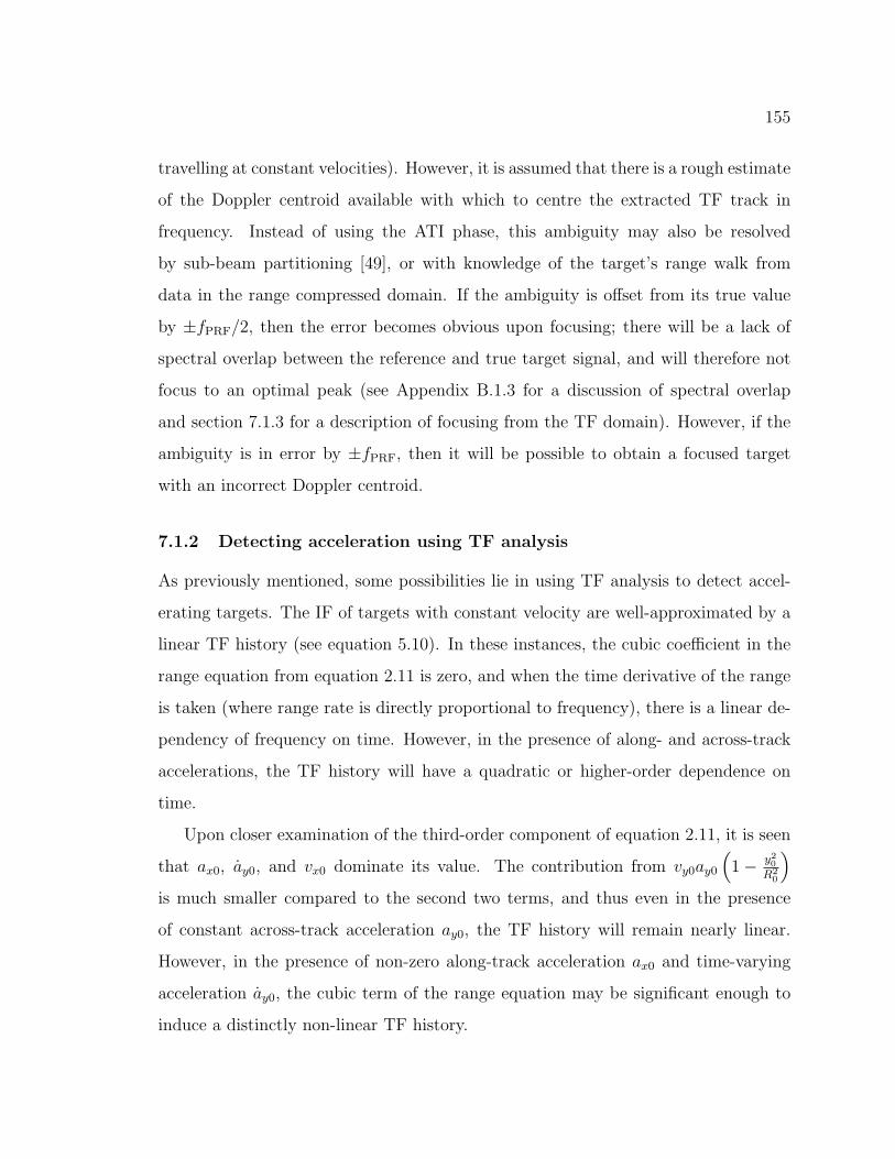
155
travelling at constant velocities). However, it is assumed that there is a rough estimate
of the Doppler centroid available with which to centre the extracted TF track in
frequency. Instead of using the ATI phase, this ambiguity may also be resolved
by sub-beam partitioning [49], or with knowledge of the target’s range walk from
data in the range compressed domain. If the ambiguity is offset from its true value
by ±fPRF/2, then the error becomes obvious upon focusing; there will be a lack of
spectral overlap between the reference and true target signal, and will therefore not
focus to an optimal peak (see Appendix B.1.3 for a discussion of spectral overlap
and section 7.1.3 for a description of focusing from the TF domain). However, if the
ambiguity is in error by ±fPRF, then it will be possible to obtain a focused target
with an incorrect Doppler centroid.
7.1.2 Detecting acceleration using TF analysis
As previously mentioned, some possibilities lie in using TF analysis to detect accel-
erating targets. The IF of targets with constant velocity are well-approximated by a
linear TF history (see equation 5.10). In these instances, the cubic coefficient in the
range equation from equation 2.11 is zero, and when the time derivative of the range
is taken (where range rate is directly proportional to frequency), there is a linear de-
pendency of frequency on time. However, in the presence of along- and across-track
accelerations, the TF history will have a quadratic or higher-order dependence on
time.
Upon closer examination of the third-order component of equation 2.11, it is seen
that ax0, ay0, and vx0 dominate its value. The contribution from vy0ay0
(1− y2
0
R20
)is much smaller compared to the second two terms, and thus even in the presence
of constant across-track acceleration ay0, the TF history will remain nearly linear.
However, in the presence of non-zero along-track acceleration ax0 and time-varying
acceleration ay0, the cubic term of the range equation may be significant enough to
induce a distinctly non-linear TF history.

156
Polynomial fits to the instantaneous frequency provide a method of detecting ax0
and ay0. One may fit a quadratic (i.e. parabola) to the IF of a target and determine
whether or not there is a significant second-order term. However, it is difficult to the-
oretically determine the threshold at which the quadratic coefficient is ‘significant’;
this depends on the SCR, CNR, and probability density function of the clutter, plus a
small second-order coefficient is expected in any case (terms smaller than 1/R20 were
dropped in Taylor series expansion of equation 2.11, but are actually still present).
The acceleration detection threshold will also be constrained by the acceptable prob-
ability of false alarms. The statistical modelling required for significance testing is
beyond the scope of this research, although it represents a potential area for further
study.
A similar approach to acceleration detection could be used in the one-dimensional
(1-D) time domain without any transformation into time-frequency space. In this
case, a cubic polynomial may be fit to the extracted DPCA phase history of the
target, and a threshold may be used to determine whether or not there is a significant
third-order component. However, due to the wide bandwidth of noise in the TF
domain (section 2.4.2), it is expected that time-frequency analysis may provide some
advantage over the 1-D time domain for detecting accelerating targets, particularly
at low SCRs.
In order to compare acceleration detection in the 1-D time and 2-D time-frequency
domains, the IF may be integrated over time to estimate the target phase history ϕ(t).
A third-order polynomial may then be fit to each phase history, and the mean and
variance in each estimate of the cubic coefficient examined. Section 7.2.2 describes
the results of simulations of acceleration detection, including comparisons using phase
histories derived in each domain.

157
7.1.3 Focusing using TF Analysis
The objective of this section is to find a method of generating SAR images of moving
vehicles that does not require knowledge of the vehicle’s motion parameters. Focusing
a moving target is possible if the phase modulation induced on the signal by the
radar-target relative motion can be determined [5]. Provided that the target signal
is sufficiently strong in the DPCA image such that the instantaneous frequency may
be reliably estimated, the IF may be used to compute this phase modulation [5].
Barbarossa was one of the first researchers to propose a scheme for detecting and
focusing moving targets based on joint TF analysis [5]. He put forward one technique
in which the instantaneous phase is used in a matched filter to obtain a focused image
[5, 7], where the instantaneous phase ϕ(t) is evaluated by integrating the estimated
frequency track through time. The integration of a discrete TF track is given by:
ϕ(t) =1
fPRF
t∑t′=−T/2
f(t′) |t| ≤ T
2, (7.2)
where T is the synthetic aperture length in units of time, and f(t) is the target IF at
sampled times t = n/fPRF for integer n. Apart from an unimportant constant term,
the resulting phase from equation 7.2 is a replica of the target phase history.
The reference signal is then exp(jϕ(t)); the time-reverse complex conjugate of
this reference is convolved with the target signal to focus a moving target [29]. Rieck
[67] has demonstrated the use of this technique to focus a moving vessel using multi-
channel SAR data. The advantage of this method is that it does not require any
assumptions regarding the type of phase modulation on the signal (e.g. quadratic,
cubic, etc. ) [5], and thus it may be used to focus accelerating targets or targets
with even higher-order motion components. This method may also be used to focus
moving targets distributed over multiple resolution cells if a rigid body assumption
may be used such that the entire target possesses the same motion.

158
7.2 Simulations
Simulations were conducted to verify the IF tracking, acceleration detection, and
focusing algorithms described in section 7.1. An airborne geometry with radar pa-
rameters typical of the CV 580 system (see values in Table 3.1) is assumed.
7.2.1 Tracking the instantaneous frequency
To verify the ability of the tracking algorithm from section 7.1.1 to extract the in-
stantaneous frequency of a target through time, simulations were performed using
various target motion parameters and various SCRs. An example of the TF history
prior to correction of ±fPRF/2 frequency jumps for a simulated target with vx0 = 10
m/s and vy0 = 15 m/s (zero acceleration) and an SCR of 0 dB is shown in Figure
7.1. An enlarged portion of Figure 7.1 is shown in Figure 7.2, where the detected
azimuth time (s)
frequ
ency
(Hz)
−2 −1.5 −1 −0.5 0 0.5 1 1.5 20
50
100
150
200
250
300
100
200
300
400
500
600
700
800
Figure 7.1: Instantaneous frequency of a simulated target with constant velocity(vx0 = 10 m/s, vy0 = 15 m/s, SCR = 0 dB) tracked through azimuthal slow-time (inwhite), and overlaid on DPCA magnitude transformed into the TF domain using thePWVD.
frequency for each azimuth time is shown in white, clearly following the peak DPCA

159
magnitude in the TF domain. Correlated complex Gaussian clutter was simulated
azimuth time (s)
frequ
ency
(Hz)
0.7 0.71 0.72 0.73 0.74 0.75 0.76 0.77 0.78 0.79 0.8255
260
265
270
275
100
200
300
400
500
600
700
800
Figure 7.2: Enlarged portion of Figure 7.1. Instantaneous frequency of a simulatedtarget with constant velocity (vx0 = 10 m/s, vy0 = 15 m/s, SCR = 0 dB) trackedthrough azimuthal slow-time (in white). The IF track is overlaid on the DPCAmagnitude image transformed into the TF domain using the PWVD. Note that theIF tracking algorithm follows the peak DPCA magnitude response.
with a coherence (represented by ρ) of 0.95, which is a relatively conservative value
for land clutter observed from typical airborne platforms [35]. Additional information
on coherence is available in Appendix B.2.
The tracking algorithm works well for reasonable SCRs. At SCRs below -15 dB
however, the tracking algorithm breaks down as bright noise spikes in the TF domain,
diverting the tracker off of the true IF. Recall that an SCR of 0 dB means that
clutter and target signal components are equally bright, i.e. have equal reflectivity
in the range compressed domain, and thus an SCR of -15 dB is very low, below the
anticipated SCRs for ground moving vehicles [46].

160
Tracking the IF in a spaceborne geometry
The time-frequency tracking algorithm may also be applied to simulations of a space-
borne scenario. Radar/geometry parameters typical of the RADARSAT-2 scenario
(see Table 3.2) were used with a PRF of 2000 Hz and an azimuthal beamwidth of
0.4◦. The increased distance to the scatterers and the radiation-resistant hardware
used in space decreases the clutter-to-noise ratio by approximately 5 to 10 dB [46].
This increase in noise makes tracking of the IF within the 2-D TF DPCA magnitude
image more difficult, particularly for low across-track velocities vy0 which result in
low DPCA magnitudes. Although IF tracking is successful for a simulated target
with vy0 = 15 m/s (as simulated above), noise spikes in the TF domain begin to pose
a problem for vy0 < 5 m/s in the space-based case. An example of the instantaneous
frequency (before correction for ±fPRF /2 jumps) for a target with vy0 = 3 m/s and
all other motion parameters set to zero is shown in Figure 7.3. Note the errors in the
extracted target time-frequency history, which should follow a smooth line. However,
the majority of these errors could be removed with some type of filtering to ignore
isolated IF points, giving a more robust TF track.
7.2.2 Detecting acceleration using TF analysis
Having established the effectiveness of the IF tracking algorithm, the acceleration
detection techniques suggested in section 7.1.2 are now evaluated. Simulations were
performed with non-zero ax0 and ay0 to examine the magnitude of the third-order
coefficient for an accelerating target. The objective was to determine whether or not
this cubic component in the range equation is discernible such that the acceleration
may be detected, even if the target is embedded in strong background clutter.
An approximation of the third-order component can be computed by fitting a cubic
polynomial to the target’s DPCA phase directly. However, as previously mentioned,
the wide bandwidth of noise in the TF domain is expected to prove advantageous
over the 1-D time domain for detecting accelerating targets at low SCRs.

161
azimuth time (s)
frequ
ency
(Hz)
−0.4 −0.3 −0.2 −0.1 0 0.1 0.2 0.3 0.40
100
200
300
400
500
600
700
800
900
2
4
6
8
10
12
14
16
18
Figure 7.3: Instantaneous frequency of a simulated target in a spaceborne geome-try with slow constant velocity (vy0 = 3 m/s and SCR = 0 dB) tracked throughazimuthal slow-time (in white). The IF track is overlaid on the DPCA magnitudeimage transformed into the TF domain using the PWVD. Low coherence and lowDPCA magnitudes introduce errors in the extracted IF track.

162
In order to perform a fair comparison between the TF and 1-D time domains,
it was ensured that no a priori information was introduced into either technique.
For this reason, the thresholding operation used to filter TF pixels before the IF
estimation stage (see section 7.1.1) was removed for these simulations, although this
may degrade the IF tracking operation by capturing bright noise spikes.
Monte Carlo simulations
Monte Carlo simulations were conducted for accelerating and non-accelerating point
targets at a variety of SCRs. The Monte Carlo method solves a problem by generating
a large number of trial runs, and then observes the fraction obeying some property
or properties. This technique is useful in obtaining a numerical solution to problems
too complicated to solve analytically [88].
A constant velocity target with vy0 = 1 m/s and vx0 = 10 m/s was simulated in
addition to an accelerating target with vy0 = 1 m/s, vx0 = 10 m/s, and ax0 = 0.5
m/s2. A non-zero vy0 was chosen such that the DPCA magnitude signal was non-zero
over the course of the observation interval (see Chapter 3). The SCR was varied from
-10 to 30 dB in steps of 2 dB. Two hundred realizations of each target at each SCR
were created in order to generate a statistically significant sample.
An airborne scenario was assumed with radar and geometry parameters given by
Table 3.1. Correlated complex Gaussian clutter was simulated with a coherence (ρ)
of 0.95. Assuming that the only factor contributing to decorrelation of the data is
additive noise, then coherence is related to the clutter-to-noise ratio (CNR) by:
ρ =1
1 + 1CNR
, (7.3)
such that ρ = 0.95 corresponds to a CNR of 25.6 dB. Note that CNRs for the
spaceborne RADARSAT-2 scenario are projected to be to be 5 to 10 dB lower than
the airborne scenario, resulting in coherences on the order of 0.94 [46], although lower
coherences due to image misregistration and other factors are possible.
For each realization, the DPCA target phase was unwrapped to generate the time-

163
dependent phase function ϕ(t). A third-order polynomial was fit to ϕ(t), and the
coefficients recorded. Some issues were encountered in unwrapping the DPCA phase
for high velocity targets at the given sampling frequency. If the target travels more
than λ/4 between sampling intervals in the slant-range direction (i.e. more than π
rads in a polar plot), then the unwrapping algorithm does not know in which direction
to unwrap. Additional unwrapping difficulties may occur if the target bandwidth over
the synthetic aperture exceeds the PRF. See Appendix B.1 for further discussion on
the velocity/acceleration bounds at which these problems occurs. However, neither of
the simulated targets described above had slant-range displacements exceeding λ/4
nor a bandwidth exceeding the PRF, and thus these sampling issues did not affect
the Monte Carlo simulation results.
Having estimated the third-order coefficient in the time domain, each simulated
target track was transformed into the TF domain using the PWVD. The IF was ex-
tracted using the same method as described in section 7.1.1, except for the omission
of the thresholding operation as mentioned in section 7.2.2. The IF was then inte-
grated over time to estimate the phase history ϕ(t). A third-order polynomial was fit
to the phase output from equation 7.2, and the coefficients were retained for further
analysis.
Cramer-Rao lower bound
For comparison purposes, the Cramer-Rao lower bound (CRLB) of the third-order
coefficient was estimated for each target at each SCR. The Cramer-Rao inequality
provides a lower bound on the variance of an unbiased estimator [40, 44]:
〈(θ − θ)2〉 ≥ 1
〈[
ddθ
ln p(x; θ)]2〉 , (7.4)
where 〈·〉 is the expectation operator, θ is the true value of the parameter, θ is
its estimate, p(x; θ) is the probability density function of variable x dependent on
parameter θ, and the right-hand side of the equation is the minimum achievable
variance. Ristic and Boashash [69] have derived the CRLBs of a signal with constant
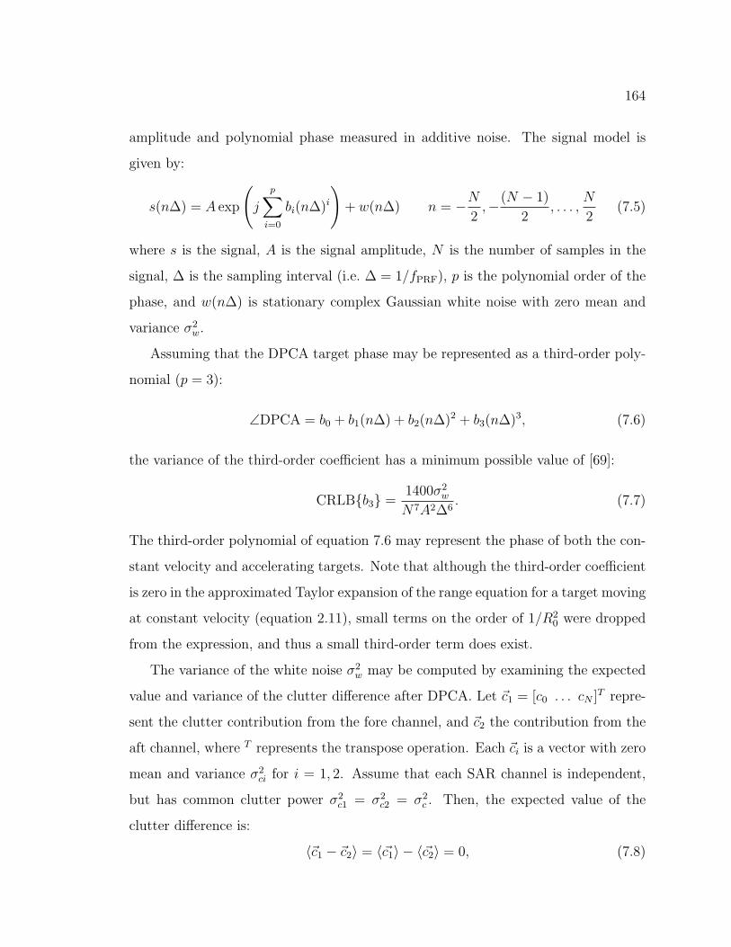
164
amplitude and polynomial phase measured in additive noise. The signal model is
given by:
s(n∆) = A exp
(j
p∑i=0
bi(n∆)i
)+ w(n∆) n = −N
2,−(N − 1)
2, . . . ,
N
2(7.5)
where s is the signal, A is the signal amplitude, N is the number of samples in the
signal, ∆ is the sampling interval (i.e. ∆ = 1/fPRF), p is the polynomial order of the
phase, and w(n∆) is stationary complex Gaussian white noise with zero mean and
variance σ2w.
Assuming that the DPCA target phase may be represented as a third-order poly-
nomial (p = 3):
∠DPCA = b0 + b1(n∆) + b2(n∆)2 + b3(n∆)3, (7.6)
the variance of the third-order coefficient has a minimum possible value of [69]:
CRLB{b3} =1400σ2
w
N7A2∆6. (7.7)
The third-order polynomial of equation 7.6 may represent the phase of both the con-
stant velocity and accelerating targets. Note that although the third-order coefficient
is zero in the approximated Taylor expansion of the range equation for a target moving
at constant velocity (equation 2.11), small terms on the order of 1/R20 were dropped
from the expression, and thus a small third-order term does exist.
The variance of the white noise σ2w may be computed by examining the expected
value and variance of the clutter difference after DPCA. Let ~c1 = [c0 . . . cN ]T repre-
sent the clutter contribution from the fore channel, and ~c2 the contribution from the
aft channel, where T represents the transpose operation. Each ~ci is a vector with zero
mean and variance σ2ci for i = 1, 2. Assume that each SAR channel is independent,
but has common clutter power σ2c1 = σ2
c2 = σ2c . Then, the expected value of the
clutter difference is:
〈~c1 − ~c2〉 = 〈~c1〉 − 〈~c2〉 = 0, (7.8)

165
and the variance is:
var[~c1 − ~c2] = 〈(~c1 − ~c2)∗(~c1 − ~c2)〉
= 〈~c1∗~c1〉 − 〈~c1
∗~c2〉 − 〈~c2∗~c1〉+ 〈~c2
∗~c2〉
= σ2c − σ2
cρ exp(jθ)− σ2cρ exp(−jθ) + σ2
c
= 2σ2c − 2ρ cos θσ2
c .
For stationary terrain the along-track interferometric phase θ = 0, and thus:
var[~c1 − ~c2] = 2σ2c (1− ρ), (7.9)
where ρ is the scene coherence. Substituting equation 7.9 into equation 7.7, and
replacing A/σc by the SCR, we find:
CRLB{b3} =2800(1− ρ)f 6
PRF
N7SCR2 . (7.10)
Analysis of simulations
Figures 7.4 and 7.5 display the absolute mean error and inverse variance of the third-
order coefficient from 200 realizations of a constant velocity target at various signal-
to-clutter ratios. A decibel scale is used in order to emphasize the differences between
polynomial fitting to the DPCA phase directly, and fitting to the phase output from
integration of the IF. Due to the decibel scale, absolute values of the mean error are
taken to avoid taking the logarithm of a negative number.
Similarly, Figures 7.6 and 7.7 illustrate the mean error and inverse variance of
the third-order coefficient from 200 realizations of an accelerating target (vx0 = 10
m/s, vy0 = 1 m/s, ax0 = 0.5 m/s2) at various signal-to-clutter ratios. The plots
from the accelerating and non-accelerating targets are very similar; both display
the same trends as a function of SCR with regards to mean error and variance of
the third-order coefficients. Neither the polynomial fit directly to the DPCA phase
nor the polynomial fit to the output from IF integration have coefficient variances

166
−10 −5 0 5 10 15 20 25 30−70
−60
−50
−40
−30
−20
−10
0
10
20
SCR (dB)
| θ −
θ |
(dB
)
|
direct
PWVD
Figure 7.4: Absolute error in the mean value of the cubic coefficient (of a polynomialfit to the DPCA phase) for a simulated target moving with constant along-trackvelocity vx0 = 10 m/s and across-track velocity vy0 = 1 m/s, graphed as a function ofSCR. ‘Direct’ represents a polynomial fit to the DPCA phase directly, while ‘PWVD’uses integration of the IF estimated from the PWVD for polynomial fitting. Meansare generated from 200 realizations of the target at each SCR. Note the decibel scaleon both axes.

167
−10 −5 0 5 10 15 20 25 30−50
0
50
100
SCR (dB)
1/σ2 (d
B)
direct
PWVD
CRLB
Figure 7.5: Inverse variance of the cubic coefficient (of a polynomial fit to the DPCAphase) for a simulated target moving with constant along-track velocity vx0 = 10 m/sand across-track velocity vy0 = 1 m/s, graphed as a function of SCR. ‘Direct’ repre-sents a polynomial fit to the DPCA phase directly, while ‘PWVD’ uses integrationof the IF estimated from the PWVD for polynomial fitting. Variances are generatedfrom 200 realizations of the target at each SCR. The Cramer-Rao lower bound isin black for reference. Note the decibel scale on both axes; the figure format wasmodelled on figures from [68].
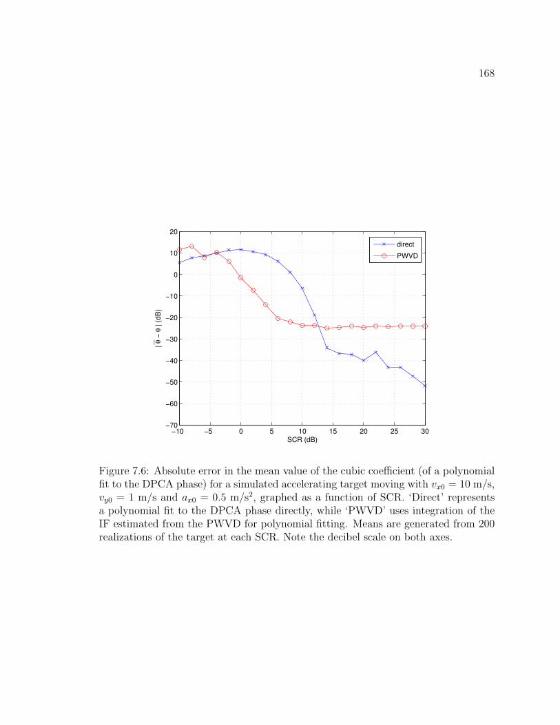
168
−10 −5 0 5 10 15 20 25 30−70
−60
−50
−40
−30
−20
−10
0
10
20
SCR (dB)
| θ −
θ |
(dB
)
|
direct
PWVD
Figure 7.6: Absolute error in the mean value of the cubic coefficient (of a polynomialfit to the DPCA phase) for a simulated accelerating target moving with vx0 = 10 m/s,vy0 = 1 m/s and ax0 = 0.5 m/s2, graphed as a function of SCR. ‘Direct’ representsa polynomial fit to the DPCA phase directly, while ‘PWVD’ uses integration of theIF estimated from the PWVD for polynomial fitting. Means are generated from 200realizations of the target at each SCR. Note the decibel scale on both axes.
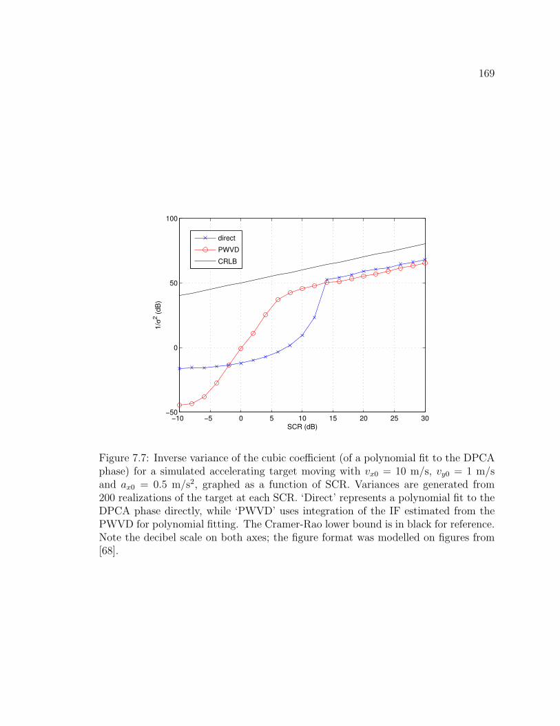
169
−10 −5 0 5 10 15 20 25 30−50
0
50
100
SCR (dB)
1/σ2 (d
B)
direct
PWVD
CRLB
Figure 7.7: Inverse variance of the cubic coefficient (of a polynomial fit to the DPCAphase) for a simulated accelerating target moving with vx0 = 10 m/s, vy0 = 1 m/sand ax0 = 0.5 m/s2, graphed as a function of SCR. Variances are generated from200 realizations of the target at each SCR. ‘Direct’ represents a polynomial fit to theDPCA phase directly, while ‘PWVD’ uses integration of the IF estimated from thePWVD for polynomial fitting. The Cramer-Rao lower bound is in black for reference.Note the decibel scale on both axes; the figure format was modelled on figures from[68].

170
approaching the Cramer-Rao lower bound, and thus neither are statistically efficient
estimators. Further analysis on the statistical properties of each technique was beyond
the scope of this research.
At very low signal-to-clutter ratios (approximately less than -2 dB), the phase
output from the IF integration has both a higher bias in the mean third-order coeffi-
cient and higher variance than integrating the phase directly, although both methods
yield relatively poor results. Improved results may be obtained using the TF method
by reintroducing the power detector threshold in the IF tracking operation, although
this makes comparisons between the direct and PWVD fitting methods inappropri-
ate. Such low SCRs may be present in range compressed data collected over urban
areas. However, as SCR increases to within the 0 to 10 dB range, there is a clear ad-
vantage to using time-frequency analysis, with lower mean errors and lower variances
in the cubic coefficient than when using the direct phase fitting technique. These
improvements are significant given the decibel scale of the plots.
The gains when using the IF to estimate phase can be attributed to reduced
contribution from the clutter noise to the tracked target signal. As discussed in
section 2.4.2, the instantaneous bandwidth of a target in the TF domain is extremely
small at any one time, while the bandwidth of the noise is much larger. After taking
the PWVD, the target energy is concentrated along one arc, whereas the noise is
spread or diluted over the 2-D time-frequency space, and therefore has less influence
on the target signal. A comparison between the phase function ϕ(t) of the unwrapped
DPCA phase, and ϕ(t) computed from the output of IF integration for a constant
velocity target with an SCR of 0 dB, is shown in Figure 7.8. Note the close agreement
between the phase determined using TF analysis and the true DPCA phase of the
target signal (uncorrupted by clutter or noise).
Signal-to-clutter ratios between 0 and 10 dB are expected to be common in realistic
scenes of moving vehicles observed from airborne and spaceborne platforms. Vehicles
moving along a highway in the experimental data (Appendix A.1) were detected with

171
−2 −1.5 −1 −0.5 0 0.5 1 1.5 2−600
−500
−400
−300
−200
−100
0
100
200
300
400
slow−time (s)
φ(t)
(rad
s)
directPWVDtrue
Figure 7.8: Unwrapped DPCA phase through azimuthal slow-time for a target with anSCR of 0 dB moving with constant velocity (vx0 = 10 m/s, vy0 = 1 m/s). Phases areshown prior to polynomial fitting for the direct case (blue) and after transformationby the PWVD and integration of the IF (red). The true DPCA phase of the targetsignal (no added clutter or noise) is given in black.

172
SCRs of between 0.6 to 10.8 dB. Note that the SCR for each vehicle was estimated
from the maximum intensity in the range compressed domain. Thirty-four sample
targets were extracted, which had a mean SCR of 6.4 dB.
As the SCR continues to increase upwards of 10 dB, the target signal sufficiently
overpowers the noise such that direct polynomial fitting to the DPCA phase is the
preferred method of estimating the third-order coefficient to obtain small errors in
the mean and small variances. Whereas the direct method continues to converge
upon the true coefficient value with increasing SCR (where a difference of −∞ in the
logarithmic scale represents zero error in the mean), the TF technique appears to be a
biased estimator of the cubic coefficient (see Figures 7.4 and 7.6). Transformation into
the TF domain is accompanied by some inevitable loss in resolution, and the tracking
operation introduces some quantization noise in determining the IF, thus limiting the
achieveable accuracy and precision in determining the third-order coefficient.
The third-order coefficient for the non-accelerating target phase had a true value
of 0.0094, whereas the cubic coefficient for the accelerating target was 18.3 dB greater
(or approximately 68 times greater) at 0.64. Thus, at high SCRs, accelerating targets
with non-zero ax0 or ay0 should be discernible from targets moving with constant
velocity.
Although beyond the scope of this work, one could assume certain probability den-
sity functions for the target and clutter signals (e.g. Gaussian target and K-distributed
clutter) in order to determine a constant false alarm rate threshold to be used for
acceleration detection. Targets whose third-order coefficients after polynomial fitting
to the phase exceed this threshold could then be flagged as accelerating targets with
a known level of confidence.
To summarize, for targets with very low SCRs TF analysis is poor at detecting
acceleration (worse than fitting a polynomial to the DPCA phase itself), for low SCRs
from 0 to 10 dB TF analysis has lower variance than using the direct phase, and for
high SCRs the direct phase is best. TF analysis is thus promising for the detection

173
of accelerating targets with medium to low SCRs although more research is needed.
Detecting acceleration in a spaceborne geometry
Theoretically the acceleration detection method used to identify significant third-
order coefficients in the airborne scenario may be applied to the space-based case.
However, as previously mentioned, CNRs in the spaceborne situation are expected to
be up to 10 dB lower than in the airborne scenario, decreasing the scene coherence
to approximately 0.94. This increased noise reduces the ability to track the IF and
accurately model the instantaneous DPCA phase, leading to errors in estimates of
the third-order coefficient and difficulties in discerning whether or not there exists
a significant third-order term. As discussed in section 4.1.2, only extremely large
cubic terms create mismatches in the reference and target signals to defocus target
responses, and thus one may not be concerned with detecting the effects of ax0 and
ay0 in the spaceborne scenario in any case.
7.2.3 Focusing using TF Analysis
As described in section 7.1.3, instantaneous phase (estimated from IF integration)
may be used to compress moving point target signals. Simulations of various tar-
get motion parameters and SCRs were conducted to test this method of focusing.
In each instance, focused images of the targets were obtained in the azimuthal di-
mension, where a focused point target appears as a narrow sinc function. Sim-
ulations concentrated on an SCR range from 0 to 10 dB, typical of real vehicle
targets observed from an airborne platform. The focused image of a simulated
target embedded in clutter with an SCR of 0 dB, and moving target parameters
[vx0 vy0 ax0 ay0 ay0]T = [10 m/s 1 m/s 0.1 m/s2 0.1 m/s2 0.01 m/s3]T is shown
in Figure 7.9. An airborne scenario was assumed with radar/geometry parameters
typical of those encountered using the CV 580 system, and the clutter was given a
coherence of 0.95. The -3 dB width of the focused response is approximately 1.0
m. The theoretical -3 dB limit for focusing a stationary target with this system is

174
−5 −4 −3 −2 −1 0 1 2 3 4 50
0.1
0.2
0.3
0.4
0.5
0.6
0.7
0.8
0.9
1
Nor
mal
ized
|DP
CA
|
azimuth (m)
Figure 7.9: Normalized DPCA magnitude of a simulated accelerating target with pa-rameters [vx0 vy0 ax0 ay0 ay0]
T = [10 m/s 1 m/s 0.1 m/s2 0.1 m/s2 0.01 m/s3]T
focused using instantaneous phase from IF integration. An SCR of 0 dB and a cluttercoherence of 0.95 were modelled. Note the narrow sinc response with a -3 dB widthof approximately 1.0 m.

175
0.47 m. Transformations into the TF domain and decorrelation of the clutter due to
additive noise create a slight loss in resolution. As well, changes in the chirp rate of
the received echo due to target motion may impact the azimuthal resolution of the
system by increasing or decreasing the available target bandwidth (see section 4.1.3).
For comparison, the same simulated moving target was focused using conventional
SAR azimuth processing (i.e. a reference filter assuming zero velocity and accelera-
tion), and the compressed image is shown in Figure 7.10. Note the severe degradation
in resolution (with a -3 dB width of 16 m) and the decrease in peak power (where
the DPCA magnitude was normalized by the same factor as that in Figure 7.9).
−50 −40 −30 −20 −10 0 10 20 30 40 500
0.05
0.1
0.15
0.2
Nor
mal
ized
|DP
CA
|
azimuth (m)
Figure 7.10: Normalized DPCA magnitude of a simulated accelerating target with pa-rameters [vx0 vy0 ax0 ay0 ay0]
T = [10 m/s 1 m/s 0.1 m/s2 0.1 m/s2 0.01 m/s3]T
focused using conventional SAR processing (i.e. assuming a stationary target). AnSCR of 0 dB and a clutter coherence of 0.95 were modelled. Note the broad andsmeared response with a -3 dB width of approximately 16 m. DPCA magnitudeswere normalized by the same factor as in Figure 7.9 for comparison purposes.
Focusing in a spaceborne geometry
Theoretically, this method of focusing may also be used to focus targets in the space-
borne case. However, as discussed in the latter portion of section 7.2.2, the decreased

176
clutter-to-noise ratios in the space-based scenario decreases scene coherence such that
may be difficult to track the IF through azimuthal time due to large noise spikes in the
2-D TF domain. For the simulated target from section 7.9 with [vx0 vy0 ax0 ay0 ay0]T =
[10 m/s 1 m/s 0.1 m/s2 0.1 m/s2 0.01 m/s3]T and an SCR of 0 dB, the time-
frequency history of the target could not be successfully tracked for a spaceborne
geometry and noise level. The problem is that vy0 is only 1 m/s, and thus the
DPCA magnitude is very low. Unless the CNR and SCR of the target under con-
sideration are unusually large, focusing using the IF track will be successful in the
RADARSAT-2 spaceborne case only for targets with at least moderate across-track
velocities (e.g. vy0 > 5 m/s).
7.3 Experimental Results
Experimental data were examined in the TF domain with the goal of detecting and
focusing accelerating targets. The data were collected during an experiment con-
ducted at Canadian Forces Base (CFB) Petawawa with the CV 580 C-Band SAR.
The experimental set-up and further results are described in Appendix A. A detection
and tracking algorithm in the range compressed domain using the DPCA technique
for clutter suppression was employed to extract and store the signal history of each
target (see section 3.3).
7.3.1 TF transform
After clutter suppression, the PWVD was applied to each control target to transform
the data into the time-frequency domain. The PWVD was chosen due to its high
TF resolution compared to linear methods, and its ability to attenuate cross-terms
between the signal and noise components. When the standard WVD algorithm was
applied to the experimental data, the noise terms made tracking of the instantaneous
frequency through time much more difficult than compared with the PWVD.
Time-frequency operations were performed using a freely-available toolbox of

177
MATLAB functions developed by Auger et al. at the CNRS (Centre National de
la Recherche Scientifique) in France and at Rice University [2]. Because the target
tracks were extracted individually prior to taking the TF transform, we expect to see
only one target in each TF image. An example of the magnitude of the DPCA signal
from a vehicle target in the TF domain is shown in Figure 7.11. The next section con-
tinues by extracting the frequency history for each target from the two-dimensional
TF image.
azimuth time (s)
Freq
uenc
y (H
z)
−2 −1 0 1 2 3 4 50
50
100
150
200
250
1
2
3
4
5
6
7
8
9
10
x 105
Figure 7.11: DPCA magnitude of a target track (l1p9 Convoy) in the time-frequencydomain after application of the PWVD.
7.3.2 Tracking the instantaneous frequency
The IF tracking algorithm for point targets described in section 7.1.1 was applied to
each of the controlled movers. The corner reflectors and vehicles being tracked in
the experimental data are reasonable approximations of point targets, such that one
should be able to reduce the IF to a single resolution cell for each azimuth time.

178
As an example of the TF history of a target from experimental data, the final IF
track for the target from Figure 7.11 is shown in Figure 7.12 after application of the
IF extraction algorithm. Note that the TF track does not appear perfectly linear;
this IF behaviour will be further examined in sections 7.3.3 and 7.3.4.
−1 0 1 2 3 4 5
200
250
300
350
400
450
500
azimuth time (s)
frequ
ency
(Hz)
Figure 7.12: Instantaneous frequency of a vehicle target (l1p9 Convoy) through az-imuth time. This frequency history was extracted from the TF image of Figure 7.11and corrected for ±fPRF /2 wraps.
Centring the IF in time
One additional step was performed on the experimental data in order to correctly
centre the target track about the time-axis. A time of t = 0 is chosen to be broadside
(denoted t0). If the complete target track for each target is collected (as can be
assumed for simulated targets), then one has only to find the mid-point of the target
track through time, and assign this as broadside. However, in experimental data the
extracted target track may not be symmetrical, and assuming that the mid-point is
t0 may result in an erroneous estimate of broadside time.
In this work, t0 is determined by cross-correlating the antenna gain pattern with
a polynomial fit of the DPCA signal magnitude (where DPCA magnitude is a scaled

179
version of the gain pattern nearly constant over the course of one synthetic aper-
ture, see Chapter 3). The time of maximal correlation is then determined, which
should be approximately equal to broadside time. A polynomial fit to the DPCA
magnitudes is used since the received signal amplitudes are noisy; when the DPCA
magnitudes are input directly into the correlation algorithm, local peaks rather than
the apparent centre of the parabolic forms are selected as broadside. One problem
with this technique is that the gently sloping gain pattern (see Figure 7.13) does not
provide a sharp correlation peak, and thus some errors in the estimated broadside
location are expected. As well, small changes in the DPCA magnitude over the course
of the synthetic aperture due to target along-track velocities and along- and across-
track accelerations (see Chapter 3) will contribute additional errors to the correlation
matching. This technique also assumes that there is no aspect-angle dependence on
the signal amplitude. This may be realistic for corner reflectors, although vehicles
may display slight changes in their RCS over the azimuthal beamwidth. These errors
may give inaccurate estimates of vy0 velocity, but they will not significantly affect
the detection of acceleration, nor the focusing of moving targets since they will only
change the linear component of the IF history.
7.3.3 Detecting acceleration using TF analysis
Polynomial fitting may be applied to the time-frequency tracks of the experimental
data in order to determine whether or not targets possess certain acceleration compo-
nents (specifically ax0 and ay0). Despite efforts to maintain a constant velocity during
the field trial, many of the target tracks extracted from the experimental data were
non-linear in the TF domain, indicating the presence of acceleration. For example,
examining the time-frequency history from an experimental vehicle target in Figure
7.12, it appears as if the IF is a combination of several linear segments. Further
insight into the target motion may be revealed using polynomial fits to the frequency
history and analysis of the residuals between these fits and the extracted IF.

180
−3 −2 −1 0 1 2 3−6
−5
−4
−3
−2
−1
0
azimuth angle off broadside (degrees)
Ant
enna
gai
n (d
B)
Figure 7.13: Antenna gain pattern of the receiving fore antenna for the CV 580system. Note the parabolic shape which does not provide a sharp correlation peak atbroadside.
Polynomials of various orders were fit to the time-frequency tracks of experimental
targets. The majority of target TF tracks had significant second-order components in
their polynomial fits, which suggests the presence of target acceleration. To compare
the results from the experimental data to those from the simulated targets in section
7.2.2, the IF frequency was integrated to determine the phase, and a third-order
polynomial was fit to this phase function. Comparisons of the twenty-two target
signals to nearby clutter revealed a mean SCR of 10.8 dB, and the mean absolute
value of the cubic coefficient was 1.17. Note that the SCR for each target track was
estimated from the maximum intensity in the range compressed domain. Recall that
each target was equipped with a corner reflector, which is why the SCR is higher
than for typical road vehicles. Note the large mean third-order coefficient in the
experimental data, which is nearly twice the value of the cubic coefficient from the
simulated target with ax0 = 0.5 m/s2 at a similar SCR, suggesting the presence of
significant target acceleration.
Differences between the target TF history and polynomial fits to this history for

181
the sample vehicle from Figure 7.12 are shown in Figure 7.14. A suitable model for
Figure 7.14: Differences between a target’s TF track f(t) and its linear fit over time(top), its quadratic fit over time (middle), and its cubic fit over time (bottom). Thetarget is l1p9 Convoy. Note the change in scale of the y-axis in the bottom frame. Thetrends in the residuals indicate the existence of higher-order uncompensated phaseterms in the data.
the target TF history would show residuals randomly distributed about zero. A linear
fit (assuming a target with constant velocity and/or constant vx0 and constant ay0)
is a clearly a poor model of the IF based on the large residuals displayed in the top
frame of Figure 7.14. However, even after compensation of ax0 and ay0 with a second-
order TF fit (see middle frame of Figure 7.14) there exist trends in the residuals,
indicating the presence of higher-order terms in the TF track. A cubic fit to the TF
history somewhat reduces the magnitude of the residuals (see bottom frame noting
the scale change in the y-axis), but deterministic (possibly sinusoidal) trends still

182
persist, revealing a complex (higher-order) TF history for this target.
There are several possible sources for these higher-order variations in the IF track.
Carrara suggests that the primary causes of phase variations (which lead to time-
varying Doppler frequency shifts) are due to uncompensated target and sensor motion,
and approximations in the image formation algorithm [12]. Improvements in the
motion compensation procedures and channel balancing algorithms used to process
the airborne experimental data are in the process of being implemented at the time of
writing. Additional time-variations in the TF track may result from target vibration
and rotation, fluctuation of the rotation centre, inaccuracy in tracking the phase (or
frequency) history, and other variations in the system and the environment [16].
7.3.4 Focusing using TF Analysis
Focusing using instantaneous phase as described in section 7.1.3 was attempted for
the experimental data. For each target track, the instantaneous phase was computed
and a matched filter of the form exp(jϕ(t)) was constructed for azimuth compression.
The reference filter was then convolved with the target signal to focus each moving
target.
To further emphasize the non-linearity and higher-order behaviour of the TF his-
tory of experimental targets, several matched filters were constructed based on various
orders of polynomial fits to the IF. Each polynomial fit was then integrated through
time to obtain an estimate of the instantaneous phase for use in matched filtering.
Figure 7.15 shows the focusing achieved for the vehicle target from Figures 7.12 and
7.14 using three different filters. In the first case (top frame) a reference filter based
on a linear fit to the time-frequency history (which assumes no along-track acceler-
ation nor time-varying across-track acceleration) was used. The extended sidelobes
to one side of the peak response suggest the presence of uncompensated cubic terms
in the target phase function [12]. In the second case (middle frame) a reference filter
based on a third-order polynomial fit was used (which accounts for acceleration terms

183
Figure 7.15: DPCA magnitudes of a vehicle target (l1p9 Convoy) focused usingmatched filters derived from various TF histories. Top: focused from a linear(first-order) fit to frequency history f(t). Middle: focused from a third-order poly-nomial fit to f(t). Bottom: focused from IF track f(t) as extracted from the PWVDdistribution. Note the superior focusing achieved using the extracted time-frequencytrack as opposed to a polynomial fit of the IF.

184
up to ay0 and ax0). In the final case (bottom portion of Figure 7.15), the extracted
time-frequency track itself (no polynomial fit) was summed to determine the phase
history. The -3 dB width of the azimuth response when focused using the IF track
itself is 0.7 m, which is on the order of the expected azimuth resolution of the CV
580 system (quoted as approximately 0.8 m [46] when system noise, system losses,
and energy loss due to the antenna gain patterns are taken into account).
Differences between the third-order TF track and the extracted TF target track
could be caused by target manoeuvring, rotation, vibration and higher-order acceler-
ation terms as well as uncompensated sensor motion. Thus, although target focusing
is improved using a third-order polynomial fit over a linear one, even higher-order ac-
celeration terms are present, and the best resolution is achieved using the extracted
TF target track itself.
The experimental data have shown that azimuth focusing is extremely sensitive to
residual phase deviations from the reference filter. Focusing using the instantaneous
phase offers marked improvements over focusing using stationary world matched filters
or filters initialized with vx0 and vy0 estimated from Chapters 5 and 6. For instance,
note the sharpened focus of the l1p9 Convoy target in the bottom frame of Figure 7.15
compared to the response from the SWMF in Figure 4.18. Substantial improvements
in focusing are also obtained using the instantaneous phase instead of a reference
filter initialized with vx0 and vy0, whose azimuth compressed response is shown in
Figure 7.16.

185
−100 −50 0 50 1000
0.02
0.04
0.06
0.08
0.1
0.12
0.14
0.16
0.18
azimuth (m)
|DP
CA
|
Figure 7.16: DPCA magnitude of a vehicle target (l1p9 Convoy) focused using areference filter initialized with vx0 and vy0 computed from a matched filter-bank andfrom the ATI phase, respectively. Note the severely smeared response and decreasedpeak power compared to focusing using the instantaneous phase in the bottom frameof Figure 7.15
.

186
Chapter 8
Conclusions and extensions
8.1 Conclusions
This research has examined the influence of acceleration on detection, focusing, and
velocity estimation of targets in dual-channel SAR-GMTI data. Although conven-
tional GMTI analysis assumes that targets travel with constant velocity, both con-
stant and time-varying accelerations have detrimental effects on target focusing and
velocity estimation if left uncompensated.
Detection
It was shown that detection of moving targets using the displaced phase centre an-
tenna (DPCA) technique is not significantly affected by acceleration. Targets moving
with non-zero across-track velocity several metres per second away from the blind
velocities have non-zero DPCA magnitudes which may be used to detect and track
the targets through azimuth time.
Focusing
However, acceleration has considerable impact upon focusing. The significant loss
of peak power, azimuthal shift, and azimuthal smearing caused by acceleration were
demonstrated. Across-track acceleration uncompensated in the reference filter during
azimuth compression severely smears the target response. This effect is identical to
the consequence of an uncompensated along-track velocity upon focusing. However,
the smearing due to across-track acceleration can be eliminated using a filter-bank to
determine the quadratic coefficient of the reference filter giving the highest magnitude
response. The primary effect of along-track acceleration and time-varying across-track

187
acceleration is the creation of asymmetric sidelobes to one side of the peak response,
which may be mistakenly identified as secondary targets in the azimuth compressed
imagery. These asymmetric sidelobes may also mask weak targets located close by.
Velocity Estimation
The effects of acceleration on velocity estimation were explored using a bank of
matched filters and along-track interferometric (ATI) phase to estimate the along- and
across-track components, respectively. Estimation of along-track velocity is severely
biased in the presence of even slight across-track acceleration (e.g. less than 0.1 m/s2)
under a constant velocity assumption. However, even if one acknowledges the possibil-
ity of acceleration, there are insufficient degrees of freedom to solve for all unknowns
with dual-channel SAR data, and thus across-track acceleration and along-track ve-
locity cannot be separated. Along-track acceleration and time-varying across-track
acceleration smear the filter-bank response, making identification of the appropriate
filter and corresponding along-track velocity more difficult.
The effects of acceleration on across-track velocity estimated using the ATI phase
were shown to be minimal as long as there is spectral overlap between the target
signal and reference filter. The best estimates of across-track velocity are derived in
the presence of complete spectral overlap, such that a bank of matched filters or an
iteration scheme is recommended for increased accuracies in velocity estimation.
Spaceborne geometries
The impacts of acceleration on GMTI data were primarily considered from an airborne
geometry due to the availability of experimental data from the CV 580 airborne plat-
form. However, spaceborne geometries were also examined since the RADARSAT-2
sensor (which will operate in GMTI mode part of the time) is to be launched in
the near future. Due to changes in geometry for the spaceborne case, resulting in
a shorter synthetic aperture time, the effects of acceleration are not as severe as in
188
the airborne scenario. Many of the effects on focusing and velocity estimation of an
uncompensated third-order component in the range history (due to along-track accel-
eration and time-varying across-track acceleration) are negligible in the spaceborne
case. However, across-track acceleration will introduce an even larger bias into the
estimate of along-track velocity if a constant velocity is assumed in the space-based
scenario.
Detection of acceleration and focusing improvements
In addition to determining the effects of acceleration, it was attempted to detect
the presence of target acceleration and to obtain a focused azimuth response irre-
spective of the motion parameters. Acceleration detection and focusing methods
were suggested making use of the instantaneous frequency (IF), which may be es-
timated after transformation of the data into the two-dimensional time-frequency
domain. Polynomial fits to the IF allow the identification of along-track acceleration
and time-varying across-track acceleration by the targets’ non-linear time-frequency
histories. Equivalently, integration of the IF gives instantaneous phase, to which a
third-order polynomial may be fit and the coefficients examined for a significant cubic
component to indicate acceleration. Due to the suppression of white noise in the TF
domain, the use of the IF for acceleration detection in regions with medium to low
signal-to-clutter ratios (between 0 and 10 dB) was shown to be superior to fitting a
polynomial to the target phase directly.
Integration of the IF allows the target phase history to be reconstructed through
time. This phase history may then used in the reference filter during azimuth com-
pression to obtain a focused image of the target. Targets in simulated and exper-
imental data possessing acceleration components were presented, and were focused
using the instantaneous phase method. These acceleration detection and focusing
algorithms may also be applied in the spaceborne case for moderate across-track ve-
locities (e.g. greater than 5 m/s) such that the DPCA magnitudes are sufficiently

189
large to track the IF.
8.2 Extensions
Additional work on the detection and compensation of acceleration is required before
these detection and focusing methods may be applied operationally. Robust statistical
models must be developed for the phase and amplitude of the DPCA clutter signal,
such that the appropriate detection threshold may be chosen for a given false alarm
rate [35, 78]. Further investigation into reliable methods of phase unwrapping are
required for application of the instantaneous phase focusing algorithm, such that it
may be applied to targets whose displacements exceed the directional ambiguity over
one synthetic aperture.
Even more than detecting acceleration, it would be desirable to estimate the
complete velocity and acceleration vector of a moving target. The use of additional
a priori information such as a database of road networks may help resolve some
of the ambiguities associated with the estimation of target motion parameters. As
well, the use of additional channels of SAR data (beyond the dual-channel scenarios
examined) would provide further degrees of freedom with which to solve for the motion
parameters. The next generation of SAR systems will be equipped with phased array
antennas, allowing increased flexibility and multi-mode operations including splitting
the radar beam into multiple channels [27, 28].
To extend this research on the effects of acceleration, increasingly realistic simu-
lations incorporating inhomogeneous clutter, antenna gain patterns, and fluctuating
radar cross sections could be considered. Collecting GPS data at a higher sampling
rate, or equipping controlled movers with accelerometers or inertial sensors would
provide further insight into the range of acceleration values of interest for ground
vehicles and acceleration’s effects on experimental SAR data.
It also would be useful to examine the theoretical effects of acceleration on incom-
plete target tracks not centred about broadside, and the effects of acceleration in the

190
presence of incorrect estimates of other parameters, situations commonly encountered
in experimental data. One of the most active topics in SAR research today is bistatic
SAR in which the transmitter and receiver are at different locations, sometimes widely
separated, such as an airborne system transmitting and ground antennas receiving
[66]. Investigations of the effects of target acceleration on SAR data collected in
bistatic geometries would be beneficial to a more thorough understanding of bistatic
GMTI.
Perhaps the most important extension of this and other GMTI work is the de-
velopment of error models to estimate the confidence in detection and parameter
estimates. Such a model would require the SCR, CNR, clutter and texture char-
acteristics, system parameters, and noise levels to obtain the correct error bounds.
Attaching a level of uncertainty to each detection and estimate is required before
GMTI may find widespread use in military and civilian applications.

191
References
[1] Adams, R. A. (1995). Calculus: A complete course. Addison-Wesley PublishersLimited, third edition.
[2] Auger, F., Flandrin, P., Goncalves, P., and Lemoine, O. (1996). Time-FrequencyToolbox: Tutorial. Centre National de la Recherche Scientifique (CNRS), Franceand Rice University, USA.
[3] Bamler, R. and Just, D. (1993). Phase statistics and decorrelation in SAR inter-ferograms. Proceedings of the IEEE International Geoscience and Remote SensingSymposium (IGARSS), 3:980–984.
[4] Barbarossa, S. (1992). Detection and imaging of moving objects with syntheticaperture radar. Part 1. Optimal detection and parameter estimation theory. IEEProceedings F Radar and Signal Processing, 139(1):79–88.
[5] Barbarossa, S. and Farina, A. (1992). Detection and imaging of moving objectswith synthetic aperture radar. Part 2: Joint time-frequency analysis by Wigner-Ville distribution. IEE Proceedings F Radar and Signal Processing, 139(1):89–97.
[6] Barbarossa, S. and Farina, A. (1994). Space-time-frequency processing of syntheticaperture radar signals. IEEE Transactions on Aerospace and Electronic Systems,30(2):341–358.
[7] Barbarossa, S. and Scaglione, A. (1998). Autofocusing of SAR images based onthe product high-order ambiguity function. Proceedings of the IEE Radar, Sonarand Navigation, 145(5):269–273.
[8] Barkat, B. (2001). Instantaneous frequency estimation of nonlinear frequency-modulated signals in the presence of multiplicative and additive noise. IEEE Trans-actions on Signal Processing, 49(10):2214–2222.
[9] Blackledge, J. M. (1989). Quantitative Coherent Imaging Theory, Methods andSome Applications. Academic Press.
[10] Bock, R. K. (1998). The data analysis briefbook: Hough transform. Avail-able from: http://rkb.home.cern.ch/rkb/AN16pp/node122.html [Accessed: May10, 2004].
[11] Breit, H., Eineder, M., Holzner, J., Runge, H., and Bamler, R. (2003). Syntheticaperture imaging radar and moving targets. In Proceedings of the IEEE Inter-national Geoscience and Remote Sensing Symposium IGARSS, volume 2, pages1187–1189, Toulouse, France.

192
[12] Carrara, W. G., Goodman, R. S., and Majewski, R. M. (1995). Spotlight Syn-thetic Aperture Radar Signal Processing Algorithms. Artech House Inc.
[13] Cenzo, A. (1981). Synthetic aperture radar and digital processing: An introduc-tion. Technical report N81-18266, Jet Propulsion Laboratory, Pasadena, California,USA.
[14] Chen, V. (2002). Detection of ground moving targets in clutter with rotationalWigner-Radon transforms. In Proceedings of the European Synthetic ApertureRadar conference (EUSAR), pages 229–232, Cologne, Germany.
[15] Chen, V. (2004). Time-frequency analysis for radar imaging, target detection,and feature extraction. IEEE Radar Conference Workshop 3.2.
[16] Chen, V. and Ling, H. (1999). Joint time-frequency analysis for radar signal andimage processing. IEEE Signal Processing Magazine, 16(2):81–93.
[17] Chen, V., Lipps, R., and Bottoms, M. (2001). Radar imaging of ground movingtargets. In Proceedings of the IEEE Radar Conference, pages 426–431, Atlanta,Georgia.
[18] Chiu, S. (2002). SAR along-track interferometry with application toRADARSAT-2 ground moving target indication. In SPIE International Sympo-sium on Remote Sensing, volume 4885, pages 246–255.
[19] Chiu, S. and Sikaneta, I. (2004). Applying fractional Fourier transform to two-aperture SAR-GMTI. In Proceedings of the European SAR conference (EUSAR),Ulm, Germany.
[20] Choi, H. (1998). Signal Processing Issues in Synthetic Aperture Radar and Com-puter Tomography. PhD thesis, University of Illinois.
[21] Coe, D. and White, R. (1995). Moving target detection in SAR imagery: exper-imental results. In Proceedings of the IEEE International Radar Conference, pages644–649, Washington DC.
[22] Coe, D. J. and White, R. G. (1996). Experimental moving target detectionresults from a three-beam airborne SAR. AEU International Journal of ElectronicCommunication, 50(2):157–164.
[23] Curry, G. (1996). A low-cost space-based radar system concept. IEEE Aerospaceand Electronic Systems Magazine, 11(9):21–24.
[24] Ender, J. (1996). Detection and Estimation of Moving Target Signals byMulti-Channel SAR. AEU International Journal of Electronic Communication,50(2):150–156.

193
[25] Ender, J. (1998). Experimental results achieved with the airborne multi-channelSAR system AER-II. In Proceedings of European Synthetic Aperture Radar Con-ference (EUSAR), pages 687–690, Friedrichshafen, Germany.
[26] Ender, J. (1999). Subspace transformation techniques applied to multi-channelSAR/MTI. In Proceedings of IGARSS Session BB2, Hamburg, Germany.
[27] Ender, J., Berens, P., Brenner, A., Rossing, L., and Skupin, U. (2002). Multi-channel SAR/MTI system development at FGAN: from AER to PAMIR. In IEEEInternational Geoscience and Remote Sensing Symposium (IGARSS), volume 3,pages 1697–1701, Toronto, Canada.
[28] Ender, J. and Brenner, A. (2003). PAMIR - a wideband phased array SAR/MTIsystem. IEE Proceedings on Radar, Sonar and Navigation, 150(2):165–172.
[29] Franceschetti, G. and Lanari, R. (1999). Synthetic Aperture Radar Processing.CRC Press.
[30] Franceschetti, G., Migliaccio, M., and Riccio, D. (1995). The SAR simulation:an overview. In Proceedings of the IEEE International Geoscience and RemoteSensing Symposium (IGARSS), volume 3, pages 2283–2285.
[31] Gallop, L. (2003). Personal Communication, October.
[32] Gierull, C. H. (2001). Statistics of SAR interferograms with application to movingtarget detection. Technical report TR 2001-045, Defence Research and Develop-ment Canada - Ottawa.
[33] Gierull, C. H. (2002). Moving target detection with along-track SAR interfer-ometry - a theoretical analysis. Technical report TR 2002-084, Defence Researchand Development Canada - Ottawa.
[34] Gierull, C. H. (2003). Digital channel balancing of along-track interferometricSAR data. technical memorandum TM 2003-024, Defence Research and Develop-ment Canada - Ottawa.
[35] Gierull, C. H. and Livingstone, C. (2004). SAR-GMTI concept for RADARSAT-2. In Klemm, R., editor, The Applications of Space-Time Processing. IEE Press,Stevenage, UK.
[36] Gierull, C. H. and Sikaneta, I. (2004). Ground moving target parameter esti-mation for two-channel SAR. In Proceedings of the European Synthetic ApertureRadar conference (EUSAR), Ulm, Germany.
[37] Gierull, C. H. and Sikaneta, I. C. (2003). Raw data based two-aperture SARground moving target indication. In Proceedings of IGARSS.

194
[38] Goldstein, R. and Zebker, H. (1987). Interferometric radar measurements ofocean surface currents. Nature, 328(20):707–709.
[39] Goodman, N. A. (2002). SAR and MTI Processing of Sparse Satellite Clusters.Doctor of philosophy, Department of Electrical Engineering and Computer Science,University of Kansas.
[40] Helstrom, C. W. (1968). Statistical Theory of Signal Detection. Pergamon PressInc.
[41] Jao, J. K. (2001). SAR image processing for moving target focusing. In Proceed-ings of the IEEE Radar Conference, pages 58–63, Atlanta, Georgia.
[42] Kirscht, M. (1996). Detection and imaging or arbitrarily moving targets withsingle-channel SAR. IEE Proceedings - Radar, Sonar and Navigation, 150(1):7–11.
[43] Klemm, R. (1998). Space-Time Adaptive Processing: principles and applications.The Institution of Electrical Engineers, London.
[44] Kullback, S. (1968). Information theory and statistics. Dover Publications Inc.,New York, N.Y.
[45] Legg, J. A., Bolton, A. G., and Gray, D. A. (1996). SAR moving target detectionusing a nonuniform pri. In EUSAR Proceedings, pages 432–426, Konigswinter,Germany.
[46] Livingstone, C. (2003a). Personal Communication, October.
[47] Livingstone, C. (2003b). Multi-look solution to the GMTI ambiguity problem: Aproposed algorithm. Defence Research and Development Canada - Ottawa internalwebnote.
[48] Livingstone, C. and Sikaneta, I. (2004). Focusing moving targets/terrain imagedwith moving-target matched filters: A tutorial. Technical report TM-2004-160,Defence Research and Development Canada - Ottawa.
[49] Livingstone, C., Sikaneta, I., Gierull, C., Chiu, S., Beaudoin, A., Campbell, J.,Beaudoin, J., Gong, S., and Knight, T. (2002). An airborne synthetic apertureradar (SAR) experiment to support RADARSAT-2 ground moving target indica-tion (GMTI). Canadian Journal of Remote Sensing, 28(6):794–813.
[50] Lombardo, P. (1996). DPCA processing for SAR moving targets detection in thepresence of internal clutter motion and velocity mismatch. In SPIE Proceedings,volume 2958, pages 50–61, Taormina, Italy.

195
[51] MacDonald Dettwiler and Associates Ltd (2004). RADARSAT-2 A New Era inRemote Sensing. Available from: http://www.mda.ca/radarsat-2/ [Accessed: June20, 2004].
[52] Marple, S.L., J. (1998). Time-frequency signal analysis: issues and alterna-tive methods. In Proceedings of the IEEE-SP International Symposium on Time-Frequency and Time-Scale Analysis, pages 329–332, Pittsburgh, Pennsylvania.
[53] Moccia, A. and Rufino, G. (2001). Spaceborne along-track SAR interferometry:performance analysis and mission scenarios. IEEE Transactions on Aerospace andElectronic Systems, 37(1):199–213.
[54] Moreira, J. R. and Keydel, W. (1995). A new MTI-SAR approach using thereflectivity displacement method. IEEE Transactions on Geoscience and RemoteSensing, 33(5):1238–1244.
[55] Murray, D., Coe, D., and White, R. (1997). Experimental MTI with spacebornegeometries. IEE Colloquium on Radar Interferometry, 153(3):1–6.
[56] Nathanson, F. E., Reilly, J. P., and Cohen, M. N. (1999). Radar Design PrinciplesSignal Processing and the Environment. Scitech Publishing Inc., Mendham, NewJersey, second edition.
[57] Nohara, T. J., Premji, A.-N., and Weber, P. T. (1999). Final report: Simulator- space based radar, volume I: Requirements, design and user guide. TechnicalReport DND9802, Sicom Systems Ltd., Ottawa, ON.
[58] NovAtel Inc. (2001). OEM4 Firmware Version 1.00 User Manual - Volume 1Installation and Operation. NovAtel Inc. pg. 75.
[59] Pascazio, V., Schirinzi, G., and Farina, A. (2001). Moving target detection byalong-track interferometry. In IEEE Geoscience and Remote Sensing Symposium(IGARSS), volume 7, pages 3024–3026, Sydney, Australia.
[60] Pettersson, M. (2001). Extraction of moving ground targets by a bistatic ultra-wideband SAR. Proceedings of the IEE Radar, Sonar and Navigation, 148(1):35–49.
[61] Ran, T., Xianjun, P., Xinghao, Z., and Yue, W. (2002). Detection and estimationof moving targets based on fractional Fourier transform. In Proceedings of the 6thInternational Conference on Signal Processing, volume 1, pages 102–105, Beijing,China.
[62] Raney, R. K. (1971). Synthetic aperture imaging radar and moving targets.IEEE Transactions on Aerospace and Electronic Systems, 7(3):499–505.
[63] Raney, R. K. (1982). Processing synthetic aperture radar data. InternationalJournal of Remote Sensing, 3(3):243–257.

196
[64] Raney, R. K. (1985). Theory and measure of certain image norms in SAR.International Journal of Remote Sensing, 23(3):343–348.
[65] Raney, R. K. (1991). Considerations for SAR image quantification unique toorbital systems. IEEE Transactions on Geoscience and Remote Sensing, 29(5):754–760.
[66] Raney, R. K. (1992). Special SAR Techniques and Applications. In AGARDConference on Fundamentals and Special Problems of Synthetic Aperture Radar,pages 10–15, Neuilly Sur Seine, France.
[67] Rieck, W. (1997). Time-frequency distribution of multichannel SAR-data forautofocusing of moving targets. In Radar Conf. Publ. No. 449, pages 224–228.
[68] Rieck, W. (1998). Zeit-Frequenz-Signal-Analyse fur Radaranwendungen mitsynthetischer Apertur (SAR). PhD thesis, Rheinisch-Westfalische TechnischeHochschule Aachen, Shaker Verlag.
[69] Ristic, B. and Boashash, B. (1998). Comments on “The Cramer-Rao lowerbounds for signals with constant amplitude and polynomial phase”. IEEE Trans-actions on Signal Processing, 46(6):1708–1709.
[70] Rodriguez, E. and Martin, J. (1992). Theory and design of interferomet-ric synthetic aperture radars. IEE Proceedings on Radar and Signal Processing,139(2):149–159.
[71] Romeiser, R. and Hirsch, O. (2001). Possibilities and limitations of currentmeasurements by airborne and spaceborne along-track interferometric SAR. InProceedings of the International IEEE Geoscience and Remote Sensing Symposium,volume 1, pages 575–577, Sydney, Australia.
[72] Rosen, P., Hensley, S., Joughin, I., Li, F., Madsen, S., Rodriguez, E., and Gold-stein, R. (2000). Synthetic aperture radar interferometry. Proceedings of the Inter-national IEEE, 88(3):333–382.
[73] Schreier, G., editor (1993). SAR geocoding: data and systems. Wichmann.
[74] Sedwick, R., Hacker, T., and Marais, K. (2000). Performance analysis for aninterferometric space-based GMTI radar system. In Proceedings of the IEEE In-ternational Radar Conference, pages 689–694, Alexandria, Virginia.
[75] Sharma, J. (2003). Summary of C.H. Gierull’s target detection and parameter es-timation algorithm. Defence Research and Development Canada - Ottawa internalwebnote.
[76] Shrader, W. W. and Gregers-Hansen, V. (1990). MTI radar. In Skolnik, M. I.,editor, Radar Handbook, pages 15.1 – 15.69. McGraw-Hill Inc.

197
[77] Sikaneta, I. (2003). Airborne SAR processor. Defence Research and DevelopmentCanada - Ottawa internal webnote.
[78] Sikaneta, I. and Chouinard, J.-Y. (2004). Eigen-decomposition of the multi-channel covariance matrix with applications to SAR-GMTI. Signal Processing,84(9):1501–1535.
[79] Sikaneta, I. and Gierull, C. H. (2004). Ground moving target detection for along-track interferometric SAR data. In Proceedings of the IEEE Aerospace Conference,Big Sky, Montana, USA.
[80] Soumekh, M. (1997). Moving target detection in foliage using along trackmonopulse synthetic aperture radar imaging. IEEE Transactions on Image Pro-cessing, 6(8):1148–1163.
[81] Soumekh, M. (1999). Synthetic Aperture Radar Signal Processing with MATLABalgorithms. Wiley Interscience, New York.
[82] Soumekh, M. and Himed, B. (2002). Moving target detection and imaging usingan X-band along-track monopulse SAR. IEEE Transactions on Aerospace andElectronic Systems, 38(1):315–333.
[83] Sparr, T. and Krane, B. (2003). Time-frequency analysis of vibrating targetsin airborne SAR systems. IEE Proceedings on Radar, Sonar and Navigation,150(3):173–175.
[84] Staudaher, F. M. (1990). Airborne mti. In Skolnik, M. I., editor, Radar Handbook,pages 16.1 – 16.29. McGraw-Hill Inc.
[85] Thayaparan, T. (2000). Linear and quadratic time-frequency representations.technical memorandum DREO-TM-2000-080, Defence Research and DevelopmentCanada - Ottawa.
[86] Thompson, A. and Livingstone, C. (2000). Moving target performance forRADARSAT-2. In Proceedings of the IEEE International Geoscience and RemoteSensing Symposium (IGARSS), volume 6, pages 2599–2601, Honolulu, Hawaii.
[87] Visentin, R. L. (1988). A digital signal processing view of strip-mapping syntheticaperture radar. Master’s thesis, University of Illinois, Urbana, Illinois.
[88] Weisstein, E. W. (1999). Monte carlo method from mathworld - a wolfram web re-source. Available from: http://mathworld.wolfram.com/MonteCarloMethod.html[Accessed: May 17, 2004].
[89] Werness, S., Carrara, W., Joyce, L., and Franczak, D. (1990a). Moving targetimaging algorithm for SAR data. IEEE Transactions on Aerospace and ElectronicSystems, 26(1):57–67.

198
[90] Werness, S. A., Stuff, M. A., and Fienup, J. R. (1990b). Two-dimensional imagingof moving targetes in SAR data. In Proceedings of the 24th Asilomar Conference onSignals, Systems and Computing, paper MP5, pages 16–22, Monterrey, California.
[91] Werninghaus, R. (2004). DLR web portal: TerraSAR-X - a new approach forscience and economy. MacDonald Dettwiler and Associates Ltd., Available from:http://www.dlr.de/dlr/raumfahrt/rf-management/erdbeobachtung/terrasar-x[Accessed: June 20, 2004].
[92] White, R. and Coe, D. (1997). Detection limits for sideways looking MTI radars.In Conference Publ. No. 449, pages 434–438.
[93] Yadin, E. (1995). Evaluation of noise and clutter induced relocation errors inSAR MTI. In Record of the IEEE International Radar Conference, pages 650–655,Alexandria, Virginia.
[94] Yadin, E. (1996). A performance evaluation model for a two port interferometerSAR-MTI. In Proceedings of the 1996 IEEE National Radar Conference, pages261–266, Ann Arbor, Michigan.

199
Appendix A
Experimental data
Data were collected during an experiment conducted at Canadian Forces Base (CFB)
Petawawa with the Environment Canada CV 580 C-Band SAR in November of 2000.
The experimental set up and data processing are described below.
A.1 Experimental set up
The CV 580 system was equipped with two antennas separated in the along-track
direction. Dual-channel SAR data were collected in HH (horizontal) polarization for
eight passes. The aircraft flew in a square twice such that there were four perpen-
dicular flight lines and two passes at each aspect angle. A list of radar parameters
and airborne geometry parameters of the Petawawa 2000 data collection is provided
in Table A.1:
Table A.1: Radar and geometry parameters for CV 580 Petawawa data collection inNovember 2000.
Parameter Value
Carrier frequency (C-band) 5.30 GHzWavelength (λ) 0.0565 mIncidence angle to control targets (θinc) 38 - 57◦
-3 dB antenna beamwidth (β) 3◦
Physical antenna separation distance (d) 0.54 mfPRF/va ratio 5.14 m−1
Pixel spacing (range) (depends on θinc) 5.1 - 7.1 mPixel spacing (azimuth) 0.19 m
Three controlled movers were involved in the data campaign. Control targets were

200
equipped with GPS receivers collecting carrier-phase data (for precise position and
velocity information) and a trihedral corner reflector was mounted to each target. A
stationary GPS receiver (also recording carrier-phase information) was located on site
to provide a reference for differential GPS post-processing. Vehicle velocities ranged
between 2.5 and 18.1 m/s (i.e. between 9 and 65 km/h). The vehicles were travelling
in a low-clutter environment of primarily grassy fields and shrubs, such that target
to clutter contrasts were generally high. The corner reflectors’ bearings and elevation
angles were adjusted for each pass, such that each corner was oriented towards the
expected broadside position of the radar to increase RCS and visibility in the SAR
imagery.
Two of the controlled moving targets (denoted as ‘Delta’ and ‘Juliet’) consisted
of a corner reflector and a GPS system mounted on a cart that moved on a rail track.
These transporters were remotely controlled, engine-powered carts guided by the rail
system which were programmed to move at predetermined speeds. Figures A.1 and
A.2 show the system that was used on both Juliet (a 700 metre track) and Delta (a
650 metre track).
A four-vehicle convoy was also deployed travelling at a relatively constant speed
along a straight segment of Veritable Road (a rough gravel road crossing the military
base). The four vehicles used are shown in Figure A.3. Although the entire convoy
was travelling at approximately the same speed, the latter three targets (labelled
two through four in the figure) were not used in the analysis because they were
not equipped with GPS receivers, and thus there is no reliable ‘truth’ information
regarding their positions and velocities over time. The pick-up truck labelled as
vehicle number one in Figure A.3 is hereafter referred to as ‘Convoy’. A photo mosaic
of the Petawawa site used in the experiment is shown in Figure A.4, with the target
tracks of the controlled movers shown in red. Vehicles on the Trans-Canada Highway
(also visible in Figure A.4) were available as targets of opportunity, although highway
targets were not examined here due to a lack of ground truth.

201
Figure A.1: Delta control target from the Petawawa 2000 data collection ( c© DRDCOttawa).
Rock Gravel
Sand
Brick wall
GPS antenna Velocity Corner reflector
Transporter
Figure A.2: Sketch of Juliet and Delta moving target rail systems with their sur-rounding structure and environment ( c© DRDC Ottawa).

202
Figure A.3: Four vehicle convoy from the Petawawa 2000 data collection ( c© DRDCOttawa).
A.2 Data pre-processing
The data delivered by the CV 580 airborne system are range compressed before being
recorded to tape, but are not azimuth compressed. This is subsequently referred to as
‘raw data’. The raw data are motion compensated and digitally balanced (in which
the amplitude and phase of both channels are matched and registered [34]) using an
in-house software package developed by Ishuwa Sikaneta at Defence Research and
Development Canada - Ottawa named SARPro (version 0.3.0) [77]. After these pre-
processing steps, the data are then passed onto the detection stage.
SARPro begins by performing an IQ balance of each channel separately, in which
it is ensured that the real and imaginary portions of the signal have zero mean and
similar variance. Next, motion compensation is applied to correct for aircraft plat-
form motion deviating from the prescribed, idealized straight-line path. If motion
compensation is not applied, processed images will be defocused and the scatterers’
will be shifted from their true positions [72].
Digital balancing (or calibration) is then performed to correct for the unavoidable

203
Figure A.4: Aerial photograph mosaic of CFB Petawawa training area, site of the 2000GMTI experiment. The tracks of the controlled movers Juliet, Delta, and Convoyare shown in red. A portion of the Trans-Canada Highway is also visible on theright-hand side.

204
channel imperfections and imbalances present in the data. These deficiencies can
be due to thermal noise in the channels, non-ideal imbalanced receiver hardware, or
different antenna gain patterns. Unmatched fore and aft channel transfer functions
result in systematic phase and amplitude terms causing errors in any subtractive
method of detection or parameter estimation such as DPCA or ATI (see section
2.3.2) [34, 79].
A routine called ‘Digibal’ (part of the SARPro package) uses a sophisticated,
adaptive two-dimensional calibration technique to simultaneously balance both mag-
nitudes and phases of the fore and aft channels. During the calibration process co-
registration is automatically performed to line-up the two channels due to differences
in the antenna phase centre locations. The algorithm works by iteratively equalizing
the channel transfer functions. Additional details on the channel balancing algorithm
are available in [34], and further information on the SARPro software package may
be found in [77].
A.3 Motion parameter estimation accuracies
This section includes details on the velocity estimation for each of the twenty-two
control target passes. The accuracies in vx0 and vy0 are broken down separately in
Tables A.2 and A.3. Along-track (vx0) velocities are computed using the filter-bank
algorithm described in Chapter 5, and across-track (vy0) velocities are computed
using along-track interferometric phase, outlined in Chapter 6. Note that line 2, pass
6 (abbreviated l2p6) only had data for the Convoy target since the Juliet and Delta
targets were stationary during imaging time due to a miscommunication with the
aircraft.
Each velocity is compared to values output from GPS; the GPS data were taken
as a best approximation of the true target motion and were used to determine the
accuracies of the parameter estimation algorithms. Technical specifications [58] cite
RMS (root mean square) accuracies of 0.03 m/s in velocity magnitudes computed

205
Table A.2: A comparison of along-track velocities (vx0) estimated using the filter-bankmethod from dual-channel SAR data and GPS. Each of the twenty-two controlledmovers in the Petawawa 2000 experiment are examined. The mean of the absolutevalue of the differences is 2.9 m/s with a standard deviation of 2.6 m/s.
Line Mover vx0 m/s vx0 m/s ∆vx0 m/s)& Pass Name (SAR) (GPS) (SAR - GPS)
l1p5 Juliet 4.37 4.52 -0.15Delta -1.94 5.99 -7.93Convoy 11.45 5.69 5.76
l1p9 Juliet 2.63 2.21 0.42Delta 1.46 5.11 -3.65Convoy 4.46 4.00 0.46
l2p2 Juliet 4.97 1.57 3.40Delta 7.43 7.57 -0.14Convoy 17.03 12.55 4.48
l2p6 Convoy 18.77 17.28 1.49
l3p3 Juliet -2.27 -2.03 -0.24Delta -1.34 -4.81 3.47Convoy -0.53 -4.13 3.60
l3p7 Juliet -0.29 -4.72 4.43Delta 4.73 -4.61 9.34Convoy -4.55 -5.36 0.81
l4p4 Juliet -3.50 -1.83 -1.67Delta -3.05 -7.52 4.47Convoy -13.70 -12.74 -0.96
l4p8 Juliet -4.04 -3.61 -0.43Delta -13.07 -9.42 -3.65Convoy -15.41 -17.37 1.96
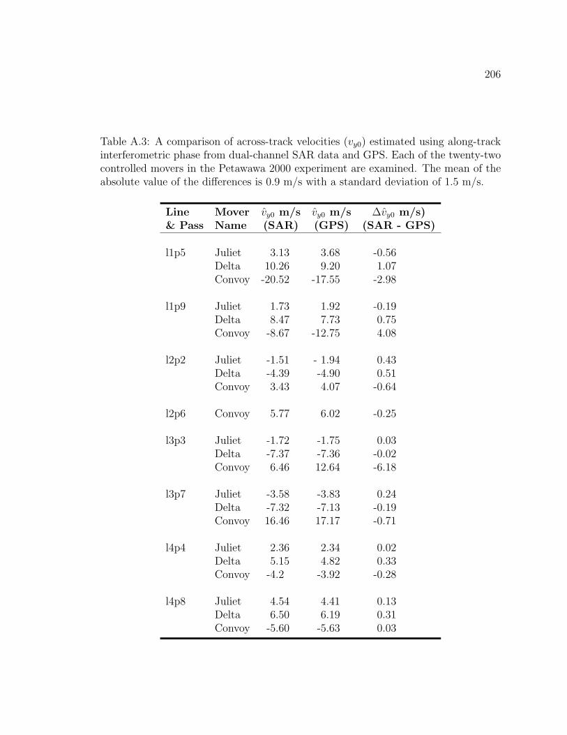
206
Table A.3: A comparison of across-track velocities (vy0) estimated using along-trackinterferometric phase from dual-channel SAR data and GPS. Each of the twenty-twocontrolled movers in the Petawawa 2000 experiment are examined. The mean of theabsolute value of the differences is 0.9 m/s with a standard deviation of 1.5 m/s.
Line Mover vy0 m/s vy0 m/s ∆vy0 m/s)& Pass Name (SAR) (GPS) (SAR - GPS)
l1p5 Juliet 3.13 3.68 -0.56Delta 10.26 9.20 1.07Convoy -20.52 -17.55 -2.98
l1p9 Juliet 1.73 1.92 -0.19Delta 8.47 7.73 0.75Convoy -8.67 -12.75 4.08
l2p2 Juliet -1.51 - 1.94 0.43Delta -4.39 -4.90 0.51Convoy 3.43 4.07 -0.64
l2p6 Convoy 5.77 6.02 -0.25
l3p3 Juliet -1.72 -1.75 0.03Delta -7.37 -7.36 -0.02Convoy 6.46 12.64 -6.18
l3p7 Juliet -3.58 -3.83 0.24Delta -7.32 -7.13 -0.19Convoy 16.46 17.17 -0.71
l4p4 Juliet 2.36 2.34 0.02Delta 5.15 4.82 0.33Convoy -4.2 -3.92 -0.28
l4p8 Juliet 4.54 4.41 0.13Delta 6.50 6.19 0.31Convoy -5.60 -5.63 0.03

207
from differentially processed GPS data such as that available in this experiment. A
summary of the statistical differences between the along- and across-track velocities
computed from the SAR data and the GPS velocities is provided in Table A.4.
Table A.4: A comparison of the absolute differences in along- and across-track ve-locities estimated using SAR data and velocities estimated from GPS. ‘Std.Dev.’represents the standard deviation.
vx0 m/s vy0 m/sAverage | SAR-GPS | 2.9 0.9Std.Dev.| SAR-GPS | 2.6 1.5
In order to separate each GPS velocity into along- and across-track components,
target heading is required. True target heading (with respect to geographic North)
was determined by subtracting adjacent GPS position estimates. True target heading
was then converted into a heading with respect to the aircraft’s line of flight using
aircraft heading from the CV 580’s GPS system. Simple trigonometry was then used
to transform each GPS speed into along- and across-track components for direct
comparison with the velocity estimates from the radar data. Table A.5 shows key
values in this conversion for each target pass, and the accuracy of the GPS along-
and across-track components is further discussed in Appendix A.3.1.
A.3.1 GPS accuracies
Errors in the GPS position estimates will result in GPS velocity and heading inac-
curacies. Typically, the greatest GPS errors occur in altitude due to the nature of
the satellite geometry (horizontally there are satellites located on almost all sides of
the targets such that some errors may cancel, whereas vertically, the satellites are all
located above the user such that errors are additive). Users of the CV 580 system
report typical RMS horizontal positional errors of between 1 to 3 metres, with vertical

208
Table A.5: Transforming GPS speed and heading into along-track and across-trackvelocities (vx0 and vy0). Bearing (i.e. heading) is abbreviated as ‘brg’, speed as ‘spd’,and ‘wrt’ represents ‘with respect to’.
Line Mover GPS GPS aircraft brg (◦) wrt vx0 vy0
& Pass Name spd (m/s) brg (◦) brg (◦) aircraft (m/s) (m/s)
l1p5 Juliet 5.83 0.2 321.0 39.2 4.52 3.68Delta 10.98 17.9 321.0 56.9 5.99 9.20Convoy 18.45 249.0 321.0 288.0 5.69 -17.55
l1p9 Juliet 2.92 2.0 321.0 41.0 2.21 1.92Delta 9.26 17.5 321.0 56.5 5.11 7.73Convoy 13.37 248.4 321.0 287.4 4.00 -12.75
l2p2 Juliet 2.49 0.0 51.0 309.0 1.57 -1.94Delta 9.01 18.1 51.0 327.1 7.57 -4.9Convoy 13.19 69.0 51.0 18.0 12.55 4.07
l2p6 Convoy 18.3 70.2 51.0 19.2 17.28 6.02
l3p3 Juliet 2.68 1.7 141.0 220.7 -2.03 -1.75Delta 8.79 17.8 141.0 236.8 -4.81 -7.36Convoy 13.3 249.1 141.0 108.1 -4.13 12.64
l3p7 Juliet 6.08 0.0 141.0 219.0 -4.72 -3.83Delta 8.49 18.1 141.0 237.1 -4.61 -7.13Convoy 17.98 248.3 141.0 107.3 -5.36 17.17
l4p4 Juliet 2.97 359.0 231.0 128.0 -1.83 2.34Delta 8.93 18.4 231.0 147.4 -7.52 4.82Convoy 13.33 68.1 231.0 197.1 -12.74 -3.92
l4p8 Juliet 5.7 0.3 231.0 129.3 -3.61 4.41Delta 11.27 17.7 231.0 146.7 -9.42 6.19Convoy 18.26 69.0 231.0 198.0 -17.37 -5.63

209
positions generally 1.5 times worse (as a rule of thumb) to give vertical accuracies of
between 1.5 to 4.5 metres [31].
Differencing the mover positions over time gives velocity and heading estimates.
However, offsets between the GPS time and the estimated broadside time of the
target could result in taking GPS measurements at the incorrect epoch. As well, GPS
measurements were collected only every 2 seconds, and the closest measurements to
the estimated imaging time were used for velocity estimation. Perhaps interpolating
GPS measurements to the nearest second would have provided small improvements in
results. If the targets were moving with constant velocity, these timing errors should
not affect GPS velocity estimates. However, in the presence of target acceleration, a
GPS measurement will have a high accuracy, but for an inappropriate time. Assuming
a maximum acceleration of 1 m/s2 and that timing errors could be incorrect by one
epoch (i.e. two seconds), this translates to a worst-case GPS velocity error of 2 m/s
for the intended time.
The theoretical accuracy in GPS heading is heavily dependent upon the speed
of the moving target being examined. At high velocities (e.g. 18.1 m/s, which was
maintained by the Convoy target), a worst-case assumption of 3 metres in horizontal
position translates to a heading error of 9.6 degrees using simple trigonometry. At
low velocities (e.g. 2.5 m/s, such as several passes for Juliet), the target moves less
than the RMS position error between epochs, and thus heading is completely unre-
liable. However, examining the GPS data, the movers’ headings displayed standard
deviations on the order of 1.5 degrees. Assuming that there are no biases in the
target GPS velocity magnitude and heading estimates, and that the aircraft heading
is known exactly, standard deviations in the speed of 0.03 m/s and in the heading of
1.5 degrees gives corresponding worst-case accuracies of 0.5 m/s in vx0 and vy0 for the
velocities and headings observed in the experimental data. This error propagation
was carried out by relating speed (|v|) and heading (α) to along- and across-track

210
velocities as follows:
vx0 = |v| sin α (A.1)
vy0 = |v| cos α. (A.2)
Partially differentiating equations A.1 and A.2 with respect to each parameter, and
squaring, summing, and taking the square root of the result gives the following ex-
pressions for standard deviations (σ) in the vx0 and vy0 velocities from GPS:
σvx0 =√
(σ|v| sin α)2 + (|v| cos ασα)2 (A.3)
σvy0 =√
(σ|v| cos α)2 + (|v| sin ασα)2, (A.4)
where σα is in units of radians.

211
Appendix B
ATI ambiguities and performance analysis
This section examines the various ambiguities present in the along-track interfero-
metric phase, and describes possible errors sources within the ATI phase. Coherence
is one crucial parameter to determining the level of phase noise in ATI SAR data,
and its derivation (assuming the presence of additive noise only) is given in Appendix
B.2.1.
B.1 ATI ambiguities
As previously mentioned, the ATI phase is subject to several ambiguities which will
effect vy0 estimation. Each type of ambiguity and its influence on the ATI phase is
discussed separately below.
B.1.1 Directional ambiguities
ATI phase can only be measured as a value between 0 and 2π (the fractional wave-
length). However, the difference in range to the target between two observations may
be several multiples of the radar wavelength, and thus the phase difference may be
several multiples of 2π, leading to an ambiguity in the ATI phase. When the difference
in the two-way propagation length to the target between observations exceeds λ/2
(i.e. |ϕ1(t) − ϕ2(t)| ≥ π, where ϕ1(t) and ϕ2(t) are the fore and aft phase histories),
the velocity direction (towards or away from the radar) becomes ambiguous. This
occurs for a displacement in slant range greater than or equal to λ/4 over the time it
takes the two apertures to spatially coincide (i.e. d/(2va) seconds for the radar-target
geometry outlined in section 2.3.1). The minimum ground displacement (Dground)

212
causing an ambiguity is then:
Dground =λ
4
1
sin(θinc), (B.1)
where θinc is the incidence angle off of vertical from the radar platform to the target.
Assuming displacement is only in the across-track direction (although this restriction
was lifted in deriving the ATI signal in section 6.1), an ambiguous ATI phase occurs
for across-track ground velocities ≥ |vambig| where
vambig =±Dground
(d/2va)=
±λva
2d sin(θinc). (B.2)
With no along-track target motion and no acceleration, ambiguities occur for across-
track velocities with magnitudes greater than 10.2 m/s for the airborne case (with
an assumed incidence angle of 40◦ and parameters given in Table 3.1) and for vy0
magnitudes greater than 44.0 m/s for the RADARSAT-2 spaceborne case (same in-
cidence angle, with geometry/radar parameters given in Table 3.2). However, these
ambiguities can be resolved by sub-beam partitioning [49], or with knowledge of the
direction of the target’s range walk from data in the range compressed domain. The
sub-beam partitioning (or ‘multi-look’ method) of ambiguity resolution separates each
target signal (from both the fore and aft channels) into fore and aft sub-beams. Each
sub-beam observes the target at different times. If the Doppler centroids of each
sub-beam are sufficiently separated such that the target focuses into separate range
bins in each sub-beam upon compression, and if there is sufficient target energy such
that the target can be detected in each sub-beam, then this provides a crude estimate
of across-track velocity useful in ambiguity resolution [47].
It may be desirable to separate the fore and aft antennae by a short distance d
such that the first ambiguous speed exceeds the maximum expected target speed [93].
However, longer antenna separations can be advantageous since they have increased
sensitivity to target motion, lowering the minimum detectable velocity, and offering
more accurate estimates of across-track velocities if the ambiguities are resolved.
There is a limit to the maximum allowable d however, as physical constraints on the

213
system size prevent the implementation of extremely long interferometric baselines in
a single pass.
B.1.2 Blind-speed ambiguities
In addition to target directional ambiguities, blind-speeds result from nλ/2 displace-
ments of the moving target in slant range over the time between apertures (for any
integer n) [47]. Targets with these displacements have an ATI phase a multiple of 2π,
which appears as a phase of zero. Such targets are difficult to detect in the raw data
domain since their DPCA phase will also be zero (see section 3.1.2), although again,
sub-beam partitioning may be used to detect and estimate the parameters of targets
moving at blind speeds. Recall from section 3.1.2 that for the CV 580 simulated
parameters, the first blind speed occurs at vy0 = 20.3 m/s, whereas the first blind
speed is vy0 = 87.9 m/s for the same target incidence angle using RADARSAT-2
parameters.
B.1.3 Doppler ambiguities
Additional ambiguities in the ATI phase occur due to the finite azimuth bandwidth
of the radar. When the two-way Doppler frequency centroid reaches ±fPRF/2, one
cannot differentiate between targets travelling towards the radar or away. When the
target spectrum has Doppler components exceeding ±fPRF/2, these components are
wrapped to the opposite side of the spectrum such that the signal becomes split
across the ±fPRF/2 boundary (see Figure 4.3) [47]. When half or more of the target
signal is wrapped, it is not apparent which portion belongs to the true target TF
representation, and which portion is wrapped. The Doppler ambiguity occurs for
across-track ground velocities ≥ |vambig Dop| where
vambig Dop =±λfPRF
4 sin(θinc). (B.3)
For signals sampled above twice the Nyquist frequency (where fnyq = 2vaβ/λ and β
is the -3 dB antenna beamwidth), this ambiguity will always occur at a larger across-

214
track velocity magnitude than the directional ambiguity discussed above. For the
airborne CV 580 case (with a PRF of approximately 642.5 Hz, oversampled above
fnyq 2.8 times) vambig Dop occurs at vy0 = ±14.1 m/s for an incidence angle of 40◦.
For the RADARSAT-2 case, the oversampling factor is dependent upon the antenna
transmit and receive beamwidths and the PRF (both of which are programmable).
This gives flexibility in the oversampling ratio from near-Nyquist sampling (i.e. 1) to
nearly 4 (i.e. at a PRF four times the clutter bandwidth), and thus vambig Dop may
vary from ±28 m/s to ±82 m/s.
However, an additional problem may occur in computing the ATI phase for a
target (compressed using a SWMF) when the signal is sampled at more than twice
the Nyquist frequency. Target motion may change the Doppler rate and shift the
Doppler centroid such that there is no spectral overlap between the target signal and
the SWMF, and thus upon compression there is no target peak. The vy0 limits within
which this occurs is dependent upon the target velocities and accelerations and the
incidence angle of observation, and thus varies across the swath and with the target
being examined. The instantaneous Doppler frequency of a target signal received by
the fore antenna is given as:
f(t) = −dφ1(t)
dt· 1
2π
= −2kdR1(t)
dt· 1
2π
= −2
λ
dR1(t)
dt, (B.4)
where a negative sign is required by the sign convention of positive Doppler frequency,
the factor of 2 accounts for the two-way range to the target, the wave number k =
2π/λ converts units from metres to radians (i.e. range to phase), and the factor of
1/(2π) converts units from radians/s into Hz.
Differentiating the Taylor expansion of the range equation (equation 2.11) with
respect to time we are left with a quadratic expression for instantaneous Doppler

215
frequency:
f(t) =−2
λ
(y0vy0
R0
+1
R0
[(vx0 − va)
2 + v2y0
(1− y2
0
R20
)+ y0ay0
]t (B.5)
+3
2R0
[vy0ay0
(1− y2
0
R20
)+ ax0(vx0 − va) +
y0 ay0
3
]t2
).
Given y0, R0 and the target motion parameters [vx0 ax0 ay0 ay0]T , one may find
vy0 such that the Doppler frequency of the target does not overlap the SWMF. The
bandwidth of the stationary reference filter is determined by setting all target mo-
tion parameters to zero in equation B.5 and evaluating f(t) at the start and end
observation times. This gives:
fsta lims =−2
λ
v2a
R0
(±T
2
), (B.6)
where fsta lims are the spectral limits of the SWMF. To find the region of zero spectral
overlap, we want to find vy0 such that the target Doppler frequency track exceeds the
SWMF Doppler limits, and to find vy0 such that when wrapped over the ±fPRF/2
limits, the spectral support of the target does not overlap the trailing/leading edge
of the SWMF (see Figure B.1 for an illustration of these boundaries). Setting the
left-hand side of equation B.5 to ±fsta lims evaluated at t = ±T/2 and solving the
quadratic for vy0 gives the start of zero overlap. Setting the left-hand side to fPRF −
±fsta lims evaluated at ∓T/2 and solving the quadratic gives the end of the zero
overlap. Between these limits, a target compressed with a SWMF will show no target
peak since there is no spectral overlap.
For the standard CV 580 parameter set with vx0 and all accelerations equal to
zero, there is no target output for ±10.2 < vy0 < ±18.0 m/s. However, increasing the
incidence angle by just ten degrees changes these limits to ±8.6 < vy0 < ±15.1 m/s.
Keeping the original incidence angle but introducing an across-track acceleration of
ay0 = −1 m/s2 changes these limits to ±8.1 < vy0 < ±20.1 m/s. As discussed in
section 6.2.6, the ATI phase should be computed by iteration or by using a bank

216
time
frequency
SWMF
Target signal v y0 > 0
Zero - overlap begins
+ PRF/2
- PRF/2
Zero - overlap ends
Wrapped target signal v y0 > 0
+ f sta . lims
- f sta . lims
Figure B.1: Example TF representation of a SWMF (in solid blue) and a targetmoving in the across-track direction with sufficient vy0 > 0 m/s such that there iszero spectral overlap between the target and reference signals (see dotted red lines).The frequency bounds at which zero spectral overlap begins and ends are delineatedfor a PRF 2.8 times greater than the clutter bandwidth (simulating the CV 580system). If vy0 increases beyond the end of zero overlap, the aliased signal will wrapback into the spectral boundaries of the reference filter.

217
of reference filters initialized with various vy0 parameters such that some spectral
overlap (and thus a target response) will be present for at least one reference filter.
The amount of spectral overlap between the target Doppler bandwidth and the
reference filter determines the magnitude of the resulting signal, and thus the mag-
nitude of the ATI phase. When there is no overlap (or very minimal overlap), the
magnitude becomes close to zero, approaching levels of the thermal noise and resid-
ual clutter, and thus the target phase may not be discernible. At target Dopplers
in excess of ±fPRF/2, the apparent frequencies of the signals become cyclic (due to
sampling they are wrapped to be within ±fPRF/2). At velocity magnitudes above
the upper zero-overlap limit, the overlap between the target and reference filter in-
creases until the wrapped Doppler centroid is equal to zero, at which point there is
maximal overlap once more with the SWMF. When the target spectrum is split over
the ±fPRF/2 boundary, the two portions of the target track will focus under SAR
processing as weak, smeared targets. Unless the target has a strong RCS, spectral
segments shorter than 1/4 of the processed bandwidth may not be detectable in the
ATI phase [47]. These ambiguities and various other match filtering issues are treated
in detail in [48].
B.2 Performance analysis
Ideally, after co-registration the two SAR channels are identical for stationary terrain
(i.e. clutter) and examining the interferogram, only moving targets should remain
in the differential data [35]. It is generally assumed that the time interval between
observations is sufficiently short to avoid the effects of time decorrelation in the scene,
and it is assumed that phase differences are due solely to changes in the slant range
to targets between epochs [53]. However, in reality, channel decorrelations do exist
such that clutter possesses non-zero ATI phase, and the target signal will always be
contaminated with clutter power [33]. If the resolution cell is larger than the target
size, pixels will contain both clutter and target components. Even if a target occupies

218
an entire resolution cell (thus masking the clutter beneath it), in the presence of an
unmatched vy0 in the reference filter, the target is shifted and superimposed on clutter
at another azimuthal location. Investigating the probability density function of the
SAR interferogram when target signals are superimposed upon clutter echoes, Gierull
found that a bias exists in the ATI phase which is dependent upon the SCR of the
received signal [33].
This relationship between SCR and ATI phase is the principal reason that ATI
phase is generally obtained in the azimuth compressed domain. The SCR is too weak
in the range compressed domain to neglect the clutter contamination. However, a
reference filter matched to the target’s quadratic component of the range equation will
increase the SCR by enhancing (focusing) the target signal and smearing the clutter,
and thus the complex sum of target and clutter components will be dominated by the
strong target signal. For parameter estimation, the ATI phase should be evaluated
only at its focused position timg after azimuth compression to reduce these clutter
contamination effects.
There are several other potential error sources in the ATI phase although system-
atic effects are the largest concern. Systematic differential phase between channels
will severely bias the ATI phase estimate. This can occur when the transfer functions
of the two channels are different and possibly varying across the swath. Unequal phase
delays through the two receiver chains, variations in the antenna phase centres with
azimuth or incidence angle, and multipath (such as the scattering of radar echoes off
the wings, fuselage, or radome in the airborne case or reflections off booms or other
structures in the spaceborne scenario) will contribute to errors in the ATI phase [72].
Adaptive channel balancing techniques which match the transfer functions of the two
channels may be used to compensate for these systematic low-frequency errors in the
data (see [34]).
Phase noise contributes additional uncertainty to the ATI phase and limits one’s
ability to detect slowly moving targets. System additive noise and speckle/internal

219
motion from the clutter causes phase decorrelation between the two channels, result-
ing in a noisy estimate of the interferometric phase of the signal of interest [86]. If
we let ρ be the correlation coefficient (also called coherence) between the two signals,
and assuming that the only factor contributing to decorrelation is additive thermal
noise, then [3, 70]:
ρ =〈z1z
∗2〉√
〈|z1|2〉〈|z2|2〉=
1
1 + 1CNR
, (B.7)
where z1 and z2 are the clutter plus noise signals from the fore and aft apertures
respectively, ∗ denotes complex conjugation, | � | denotes absolute value, 〈�〉 denotes
expectation, and CNR represents the clutter-to-noise ratio. Equation B.7 is derived
in Appendix B.2.1. As the CNR approaches infinity, the coherence goes to unity. For
single-pass ATI, coherences are normally quite high (e.g. larger than 0.95) although
they may be significantly lower for water surfaces (where ρ less than 0.80 are com-
mon) [35]. Assuming that the thermal noise contributing to a non-zero coherence is
normally distributed with mean zero and standard deviation σ given by [70]:
σ =1√2
√1− ρ2
ρ, (B.8)
then the corresponding across-track velocity noise (computed from the phase, assum-
ing no along-track motion or accelerations) is also normally distributed with mean
zero and standard deviation σvy [86]:
σvy = σλ
2π
va
d sin(θinc). (B.9)
For a coherence of 0.95, equation B.9 gives a standard deviation in vy0 of 0.8 m/s for
the airborne case and 3.2 m/s for the RADARSAT-2 scenario.
This phase decorrelation also limits the minimum detectable velocity using ATI
phase. When plotted on the complex plane, the phase of the ATI signal is the angle
measured from the positive real axis, and its magnitude is the distance from the
origin. With an ideal ‘noise-free’ radar and perfectly stationary scatterers, the clutter
is completely coherent between channels (i.e. ρ = 1) and maps to the real axis [49].

220
However, partial decorrelation of the channels over the SAR aperture results in ATI
phase measurements of stationary scene elements deviating away from the real axis
(see Figure B.2). Such decorrelation can result from additive noise in the radar
system, phase noise of the radar, and motion of the clutter over the observation
period [49]. Note that this mapping of the clutter to the vicinity of the real axis
occurs only for land clutter. On sea surfaces, the background clutter will move due to
surface waves and currents, and the ATI phase of the background will have a non-zero
average angle [78].
270
0
90
180
Q
IStationaryterrain
objectMoving
Figure B.2: Illustration of the across-track interferometric (ATI) signal in the complexplane for a moving target with accompanying clutter, where I is the inphase (real) axisand Q the quadrature (imaginary) axis. The moving target has distinctly non-zerophase, whereas (except for thermal noise near the origin) stationary terrain maps intoa statistical distribution about the positive real axis. Adapted from [49].
Stationary clutter may be suppressed in the ATI complex image by nulling the
magnitudes of all signal components whose phases lie within a given threshold of the
real axis[49]. This nulling is accomplished using a so-called ‘keyhole’ filter, whose
threshold may be chosen based on a given constant false alarm rate (CFAR) and

221
knowledge of the marginal phase distribution [32]. The minimum detectable velocity
is limited by the choice of this threshold; moving targets are identified as those data
whose phase angles are greater than that defined by the filter threshold. All ATI data
(including slow-moving targets) with phases below this threshold are assumed to be
stationary clutter and are thus removed.
Other possible sources of error in the ATI phase include atmospheric effects, al-
though these are negligible since both signals propagate through the same portion of
the atmosphere nearly simultaneously, such that ionospheric or tropospheric delays
are the same in each channel. Errors in the baseline between the two antennas would
also contribute to errors in parameter estimation from ATI phase, although in the CV
580 and RADARSAT-2 cases this baseline is very well known; baseline errors pose
more of a problem when instead of on a rigid body, antennas are placed on the wings
of an aircraft (which oscillate slightly during flight) or on a boom (whose movements
may be difficult to control), or when repeat-pass interferometry is performed. The
presence of an across-track component in the baseline (such as when the radar point-
ing angle is not orthogonal to the flight path) will introduce some phase variation due
to the topography in addition to phase differences due to target motion.
B.2.1 Coherence
A simplified expression for the correlation coefficient - often called coherence (ρ)
- between two interferometric channels of clutter is derived. Let the fore and aft
signals at any instant in time be represented by z1 and z2, respectively:
z1 = c + n1
z2 = c + n2, (B.10)
where c is the common clutter component in each channel, and n1 and n2 are noise
components in each channel. Let the clutter c be a complex random variable with
mean 0 and variance σ2c , and n1 and n2 are also complex random variables, each with

222
mean 0 and variance σ2n. We assume that the clutter and noise are independent, and
that n1 is independent from n2. Assuming that additive noise n is the only factor
contributing to scene decorrelation, the coherence is given by:
ρ =〈z1z
∗2〉√
〈|z1|2〉〈|z2|2〉, (B.11)
where ∗ denotes complex conjugation, | � | denotes absolute value, and 〈�〉 denotes
expectation.
Simplifying the numerator:
〈z1z∗2〉 = 〈(c + n1)(c + n2)〉
= 〈cc∗ + cn∗2 + n1c∗ + n1n
∗2〉
= σ2c . (B.12)
Simplifying each term in the denomentor:
〈|z1|2〉 = 〈z1z∗1〉
= 〈(c + n1)(c + n1)∗〉
= 〈cc∗ + cn∗1 + n1c∗ + n1n
∗1〉
= σ2c + σ2
n. (B.13)
〈|z2|2〉 = σ2c + σ2
n. (B.14)
Plugging in the results from B.12, B.13, and B.14 into B.11, we find the coherence:
ρ =σ2
c
σ2c + σ2
n
. (B.15)
Letting σ2c/σ
2n represent the clutter-to-noise ratio (CNR), the coherence may also be
given as:
ρ =1
1 + 1CNR
, (B.16)
which completes the derivation of equation B.7.