uav-licam system development: calibration and …...uav-licam system development: calibration and...

UAV-LiCAM SYSTEM DEVELOPMENT: CALIBRATION AND GEO-REFERENCING

C. Cortes 1,*, M. Shahbazi 1, P. Ménard 2

1 Dept. of Geomatics Engineering, University of Calgary, Alberta, Canada – (cecortes, mozhdeh.shahbazi)@ucalgary.ca 2 Centre de géomatique du Québec Inc, Saguenay, Québec, Canada – [email protected]

Commission II, WG I

KEY WORDS: UAV, Lidar, Camera, GNSS/INS, Self-calibration, Unscented Particle Filtering, Geometric Primitives ABSTRACT: In the last decade, applications of unmanned aerial vehicles (UAVs), as remote-sensing platforms, have extensively been investigated for fine-scale mapping, modeling and monitoring of the environment. In few recent years, integration of 3D laser scanners and cameras onboard UAVs has also received considerable attention as these two sensors provide complementary spatial/spectral information of the environment. Since lidar performs range and bearing measurements in its body-frame, precise GNSS/INS data are required to directly geo-reference the lidar measurements in an object-fixed coordinate system. However, such data comes at the price of tactical-grade inertial navigation sensors enabled with dual-frequency RTK-GNSS receivers, which also necessitates having access to a base station and proper post-processing software. Therefore, such UAV systems equipped with lidar and camera (UAV-LiCam Systems) are too expensive to be accessible to a wide range of users. Hence, new solutions must be developed to eliminate the need for costly navigation sensors. In this paper, a two-fold solution is proposed based on an in-house developed, low-cost system: 1) a multi-sensor self-calibration approach for calibrating the Li-Cam system based on planar and cylindrical multi-directional features; 2) an integrated sensor orientation method for georeferencing based on unscented particle filtering which compensates for time-variant IMU errors and eliminates the need for GNSS measurements.

1. INTRODUCTION

1.1 Technology Overview

Techniques of visual three-dimensional (3D) mapping are either based on passive imaging (e.g. application of photogrammetry) or active ranging (e.g. laser scanning) (Nouwakpo et al., 2015). The sensors (e.g. digital cameras or 3D light detection and ranging (lidar) sensors) can be integrated either to terrestrial mobile/static platforms or, alternatively, to aerial platforms such as manned aircrafts and unmanned aerial vehicles (UAVs). Terrestrial platforms have several advantages. For instance, their control is simpler; they have considerable payload capacity; and they are closer to the terrain, thus, the data can be acquired with higher spatial resolution. However, their access to areas of interest can be limited. In comparison with manned aerial platforms, unmanned aerial vehicles (UAVs) have recently gained higher relevance in different fields of remote sensing. This is mainly due to the fact that by integrating consumer-grade imaging and ranging sensors to UAVs, data with high temporal and spatial resolutions can be acquired at considerably lower costs and by less effort (Shahbazi et al., 2014). In several studies, investigations have been performed to compare the advantages and disadvantages of 3D reconstruction using photogrammetry versus laser scanning. The simple conclusion could be that any 3D-vision technology has its own pros and cons. There is no technology which is completely robust against all the sources of error and noise caused by sensor characteristics and/or environmental factors, such as light intensity variations, shadows, adverse weather conditions (rain, snow, mist and dust), reflectivity variations (caused by material, colour and texture), different penetration strengths, moving objects in the scene, occlusions, systematic and random errors of georeferencing, etc. Thus, depending on the application, different sensors can be fused so that their integrated data can provide a more robust performance.

Various commercial systems that incorporate both sensors (camera and lidar) within a UAV platform have recently been developed. The most popular systems, manufactured by Phoenix and Riegl, host a tactical-grade inertial navigation system (INS) that helps directly georeference the sensors data with centimetre-level accuracy. The cost of the high-accuracy INS systems drive the overall price of these systems up making them inaccessible to a large range of potential users. This paper proposes a solution that utilizes an industrial-grade INS instead to achieve similar accuracy in merging point clouds and georeferencing data. 1.2 Related Work

A key factor to maximize the geometric quality of the data acquired by a sensor is to ensure its accurate calibration and modeling of systematic errors that affect its measurements. In the case of a Li-Cam system, three basic types of geometric calibration are required: intrinsic camera calibration, intrinsic lidar calibration, extrinsic system calibration. 1.2.1. Calibration: Camera calibration using photogrammetric techniques is a well-studied topic, and the integration of digital cameras to UAVs has also been investigated extensively during the last few years (Remondino and Fraser, 2006; Shahbazi et al., 2015). The method implemented in this paper is based on the work described in (Shahbazi et al., 2017), in which a sparse free-network self-calibrating bundle adjustment (BA) is used to estimate the calibration parameters; in this work, multiple cameras are calibrated simultaneously, and the BA unknown parameters are decorrelated considerably. There are also several studies in the literature that are dedicated to the analysis of the intrinsic and extrinsic calibration of airborne laser scanners (ALS) (Habib et al., 2010). The definition of additional parameters, which are used to model systematic errors, depends mainly on the type of the lidar sensor

The International Archives of the Photogrammetry, Remote Sensing and Spatial Information Sciences, Volume XLII-1, 2018 ISPRS TC I Mid-term Symposium “Innovative Sensing – From Sensors to Methods and Applications”, 10–12 October 2018, Karlsruhe, Germany

This contribution has been peer-reviewed. https://doi.org/10.5194/isprs-archives-XLII-1-107-2018 | © Authors 2018. CC BY 4.0 License.

107

and its scanning mechanism (Glennie et al., 2016; Lichti, 2007; Glennie and Lichti, 2011, 2010; Atanacio-Jiménez et al., 2011). Apart from the intrinsic errors, other important factors are the errors of the platform position and orientation as well as the errors of system calibration (Skaloud and Lichti, 2006). Early studies of system calibration are based on recovering the misalignment of INS-lidar through signalized target points. However, target points cannot be directly recognized in an ALS point cloud due to its large point spacing and low density. That is, interpolation of the target points from the lidar point cloud (PC) limits the pointing and calibration accuracy. Comparatively, the recent methods using features of known shape are more rigorous for lidar system calibration. These methods can be broadly divided into two categories. The first category includes methods based on iterative closest point (ICP) estimation of calibration parameters through minimizing the inconsistency between the points of overlapping scan strips which are located on common features (Habib et al., 2010). The ICP solution can be computationally expensive since a high number of iterations are required and the volume of ALS data is relatively large (Chan et al., 2013). The second category includes methods based on least-square (LS) estimation of calibration parameters through conditioning points lying on specific features, e.g. planar features (Glennie et al., 2016), linear features (Le Scouarnec et al., 2014), catenary features (Chan et al., 2013), and pole-like features (Chan et al., 2015). Due to depending on INS/GPS observations, all the studies need to consider the level of uncertainty of these observations in the self-calibration adjustment and to re-perform the calibration to measure bore-sight and lever-arm uncompensated errors during the flight when the INS/GPS observations become more accurate. Another issue, reported by previous studies, is the high correlation between calibration parameters in the LS adjustment. Studies have shown that using multiple features (e.g. several planes) and multiple geometric primitives (e.g. catenary and planar features) can considerably reduce the correlation between the calibration parameters. When it comes to the UAVs as airborne lidar platforms, the calibration problem should be treated differently due to the following reasons. First, because of UAV payload limits, compact lidar sensors are built with specific mapping characteristics compared with traditional airborne lidar devices (e.g. different vertical field of view, footprint size, penetration strength, numbers of returns, density per square meter, etc.). Second, compact and low-cost GNSS-based inertial navigation systems (usually non-differential) are used for georeferencing the lidar point clouds, which have low accuracy and precision. Therefore, the calibration of UAV-based lidar systems is still an active area of research (Kasturi et al., 2016; Guerreiro et al., 2014; Tulldahl et al., 2015; Teichman et al., 2013; Wallace et al., 2012). Most of the current studies analyse the extrinsic calibration of lidar with respect to the INS. However, less attention is given to the intrinsic calibration of the sensors. Studies have also been performed for extrinsically calibrating a lidar sensor with respect to a camera, or to perform their joint calibration (e.g. Gong et al., 2013). Simultaneous internal calibration of 3D lidar and extrinsic calibration between a lidar and a Ladybug camera based on planar features was proposed in (Mirzaei et al., 2012), where a mean distance error of -0.67 mm with a standard deviation of 55 mm was achieved. Park et al. (2014) proposed using the vertices of a polygonal planar boards to find point correspondences between 2D images and 3D lidar data. For extrinsic calibration of sparse 3D lidar sensors such as Velodyne VLP-16, this method would be prone to erroneous

estimation of the polygon edges, which would propagate into the vertices calculation and, thus, would affect the estimated calibration parameters adversely. Furthermore, the edge estimation is based only on a few points and any outlier would have a significant impact on the resulting calibration parameters. 1.2.2. Georeferencing: One of the objectives of the project described in this paper is to correct the trajectory of the UAV derived from Inertial Measurement Unit (IMU) measurements using camera poses, derived via robust structure-from-motion and bundle adjustment (Shahbazi et al., 2015, 2017). As it is commonly known, the position derived from IMU measurements can rapidly drift due to accelerometer and gyroscope biases and their random walks. Since the position is derived from the integration of acceleration and angular velocity measurements, errors in these raw measurements propagate exponentially causing large errors in the estimated positions. Most inertial navigation systems integrate IMU and Global Navigation Satellite System (GNSS) measurements together using various Bayesian recursive filtering techniques to compensate for their errors. The GNSS measurements are used to estimate IMU errors and correct the position. This sensor integration works quite well when multipath-free GNSS signals can be consistently received from a good geometric configuration of satellites. However, in many cases such as urban canyons, forested areas, and indoor environments, GNSS signals are not reliable or available. In the case of low-cost UAV platforms, due to their payload and cost constrains, low-cost GNSS receivers are used whose positioning accuracy can be insufficient for certain applications. UAVs are usually equipped with digital cameras which are used to capture imagery and generate photogrammetric point clouds. One of the outputs of this process include optimized 3D position and orientation of the camera at each epoch, which even without any ground control points can have high relative accuracy. Thus, camera-based position and orientation can be strong alternate observations to be integrated with IMU measurements (if the relative orientation parameters between the IMU and digital camera are known). Particle filtering is a Bayesian recursive filtering method that can be used to accomplish this objective. As explained in (Doucet and Johansen, 2011), particle filters have several advantages over other popular methods (e.g. Extended Kalman Filter), such as its ability to yield optimal estimations with non-Gaussian believes. 1.3 System Overview

The low-cost mapping system developed in this study is equipped with a 3D spinning laser scanner (Velodyne VLP-16), a DSLR optical camera (Sony a6000), and an industrial-grade INS (VectorNav VN-200), as shown in Figure 1.

Figure 1. UAV-LiCam System



108

2. METHODOLOGY

In the case of our UAV-LiCam system, three basic types of geometric calibration are performed: intrinsic camera calibration, intrinsic lidar calibration, and extrinsic system calibration. In this approach, the camera calibration takes place separately. Once the camera calibration is accomplished and the camera is firmly attached to the system, the relative orientation parameters between the three sensors (camera, IMU, lidar) as well as the lidar intrinsic parameters are estimated simultaneously through a combined bundle adjustment. In this study, an external camera to the system (a DSLR Canon M5) is also used in the process of system calibration. Therefore, the two cameras need intrinsic calibration. The systematic errors caused by : 1) lens radial distortion; 2) lens decentring distortion; 3) affinity and non-orthogonality of sensor are modelled, and interior orientation parameters (principal point offsets and focal length) are estimated for both cameras in one adjustment procedure. The readers are referred to our previous work (Shahbazi et al., 2015 and 2017) where the details of our sparse free-network multi-camera self-calibrating bundle adjustment approach can be found. 2.1 System Calibration

Intrinsic lidar calibration involves the modelling of the systematic errors of range, elevation-angle and horizontal-direction measurements. The VLP-16 sensor includes 16 lasers, each of which has a specific set of intrinsic calibration parameters. In this study, only three intrinsic parameters are calibrated: range zero-error; horizontal circle scale error; vertical circle zero index error. The local 3D coordinates of a point (i) at time (t) measured by the j’th laser via observing range (ri,t), horizontal direction (βi,t), and elevation angle (θi,t) can be calculated as in Equation (1),

, , , ,

, , , , ,

, ,

( ) cos( )sin( )

x ( ) cos( ) cos( )

( )sin( )

i t j j i t i t j i tj j j j

i t i t j j i t i t j i tj j j j j

i t j j i tj j

r a c b

r a c b

r a c

θ β β

θ β β

θ

+ + + = + + + + +

(1)

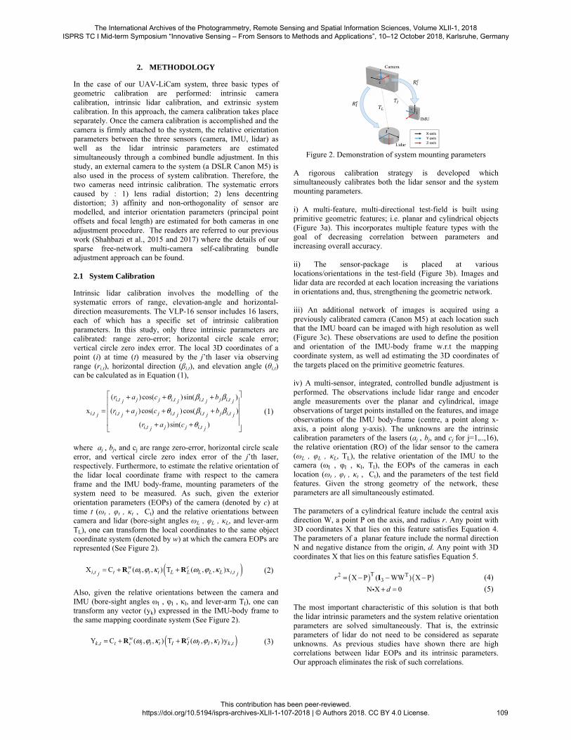
where aj , bj, and cj are range zero-error, horizontal circle scale error, and vertical circle zero index error of the j’th laser, respectively. Furthermore, to estimate the relative orientation of the lidar local coordinate frame with respect to the camera frame and the IMU body-frame, mounting parameters of the system need to be measured. As such, given the exterior orientation parameters (EOPs) of the camera (denoted by c) at time t (ωt , φt , κt , Ct) and the relative orientations between camera and lidar (bore-sight angles ωL , φL , κL, and lever-arm TL), one can transform the local coordinates to the same object coordinate system (denoted by w) at which the camera EOPs are represented (See Figure 2).

( ), ,X C ( , , ) T ( , , )xw ci t t c t t t L L L L L i tj j

ω ϕ κ ω ϕ κ= + +R R (2)

Also, given the relative orientations between the camera and IMU (bore-sight angles ωI , φI , κI, and lever-arm TI), one can transform any vector (yk) expressed in the IMU-body frame to the same mapping coordinate system (See Figure 2).

( ), ,Y C ( , , ) T ( , , )yw ck t t c t t t I I I I I k tω ϕ κ ω ϕ κ= + +R R (3)

Figure 2. Demonstration of system mounting parameters

A rigorous calibration strategy is developed which simultaneously calibrates both the lidar sensor and the system mounting parameters. i) A multi-feature, multi-directional test-field is built using primitive geometric features; i.e. planar and cylindrical objects (Figure 3a). This incorporates multiple feature types with the goal of decreasing correlation between parameters and increasing overall accuracy. ii) The sensor-package is placed at various locations/orientations in the test-field (Figure 3b). Images and lidar data are recorded at each location increasing the variations in orientations and, thus, strengthening the geometric network. iii) An additional network of images is acquired using a previously calibrated camera (Canon M5) at each location such that the IMU board can be imaged with high resolution as well (Figure 3c). These observations are used to define the position and orientation of the IMU-body frame w.r.t the mapping coordinate system, as well ad estimating the 3D coordinates of the targets placed on the primitive geometric features. iv) A multi-sensor, integrated, controlled bundle adjustment is performed. The observations include lidar range and encoder angle measurements over the planar and cylindrical, image observations of target points installed on the features, and image observations of the IMU body-frame (centre, a point along x-axis, a point along y-axis). The unknowns are the intrinsic calibration parameters of the lasers (aj , bj, and cj for j=1,..,16), the relative orientation (RO) of the lidar sensor to the camera (ωL , φL , κL, TL), the relative orientation of the IMU to the camera (ωI , φI , κI, TI), the EOPs of the cameras in each location (ωt , φt , κt , Ct), and the parameters of the test field features. Given the strong geometry of the network, these parameters are all simultaneously estimated. The parameters of a cylindrical feature include the central axis direction W, a point P on the axis, and radius r. Any point with 3D coordinates X that lies on this feature satisfies Equation 4. The parameters of a planar feature include the normal direction N and negative distance from the origin, d. Any point with 3D coordinates X that lies on this feature satisfies Equation 5.

( ) ( )23X P ( WW ) X Pr

Τ Τ= − − −I (4)

N X 0d+ = (5) The most important characteristic of this solution is that both the lidar intrinsic parameters and the system relative orientation parameters are solved simultaneously. That is, the extrinsic parameters of lidar do not need to be considered as separate unknowns. As previous studies have shown there are high correlations between lidar EOPs and its intrinsic parameters. Our approach eliminates the risk of such correlations.



109

a)

b)

c)

d)

e)

Figure 3. Calibration fields; a) system/lidar calibration field; b) stations (black frames), where data with the Li-Cam system is collected from the field of Figure 3a; c) stations (red frames), where images with the external camera are collected from the

test-field; d) camera calibration test-field; e) checkerboard panel for camera calibration accuracy validation

2.2 Georeferencing

To represent non-Gaussian probability distributions, particle filters sample multiple particles from the non-Gaussian belief. If sufficient particles are sampled, then a close approximation of the belief can be obtained. Each particle is a hypothesis of the current state. The true state lies where the highest density of particles is. Particle filters make use of importance sampling to assign a weight to each randomly sampled particle. This weight is inversely proportional to the difference between the proposal function (prediction) and the actual belief distribution (based on external measurements). The closer a particle represents the true belief, the higher its weight will be. Once a weight is assigned to every particle, a re-sampling of the particles based on their associated weights replaces the least probable particles by more probable ones. In this study, unscented particle filtering (UPF) is used to integrate the IMU measurements (3D acceleration and angular velocity) with camera observations (exterior orientation parameters as well as parameters of geometric primitives present in the scene) and lidar observations (points lying on those geometric primitives). The reason to use unscented filtering is to deal with non-linearity of both transition and measurement functions with respect to measurements, controls, and the state. The details of this approach are presented in Figure 4. The general structure of the implemented UPF is as follows: i) The state vector includes: 3D position of the lidar origin, 3D rotations of the lidar frame w.r.t. the object-fixed coordinate system, 3D velocity of the lidar, 3D bias of the accelerometer, 3D bias of the gyroscope. ii) The control data includes: 3D accelerations and angular velocities measured by the IMU. iii) The transition probability is based on kinematic motion models, and the process noises include: 3D velocity impulses, 3D rotation perturbations, random walks of accelerometer and gyroscope biases. iv) The importance weights are derived from the measurement probabilities that are based on two types of observations: lidar pose relative to known camera poses, and lidar measurements from geometric primitives, e.g. planes, present in the scene assuming that the parameters of such primitives are derived using camera observations.

Figure 4. Workflow of lidar point cloud geo-referencing using

UPF The mathematical details of UPF are avoided, and readers are referred to (Ducet and Johansen, 2010).



110

3. EXPERIMENTS

3.1 Camera Calibration

The camera calibration was first carried out separately. A calibration test field (Figure 3d) was designed based on the specifications of the Sony a6000 and Canon M5 cameras. A few targets (3 to 12) on each wall were surveyed with a total station to establish an object space coordinate system. The 3D coordinates of all the other targets were approximated via ray-casting; these approximate coordinates were only used for facilitating the target labelling without the need for coded targets and also for estimating the initial EOPs of images. 2D target observations from a total of 30 images (per camera) were then extracted using our semi-automated target detection and labelling software. An additional set of 10 images (per camera) of a calibration checkerboard panel (Figure 3e) were used to validate the accuracy of the estimated calibration parameters. 3.2 System/Lidar Calibration

The data collection for lidar and system calibration took place in an open hallway at the University of Calgary engineering building. As it can be seen in Figure 3a, circular targets were placed on all the features of interest. In total, 3 cylindrical concrete pillars and 11 different planes formed the calibration test field. These features covered an area of 4x14x3 meters at 6 different directions, including floor and ceiling. All targets were surveyed with a total station; some of these coordinates were used as control-point observations in the integrated bundle adjustment.

3.3 Georeferencing

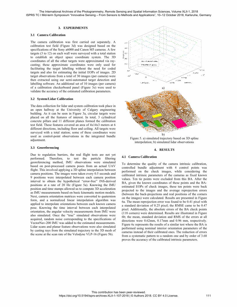
Due to regulation barriers, the real flight tests are not yet performed. Therefore, to test the particle filtering georeferencing method, IMU observations were simulated based on post-processed camera poses from an actual UAV flight. This involved applying a 3D spline interpolation between camera positions. The images were taken every 0.5 seconds and 9 positions were interpolated between each camera position interval to obtain the hypothetical “error-free” INS-derived positions at a rate of 20 Hz (Figure 5a). Knowing the IMU position and time stamps allowed us to compute 3D acceleration as IMU measurements based on basic kinematic motion models. Next, camera orientation matrices were converted to quaternion form, and a normalized linear interpolation algorithm was applied to interpolate orientations between each known camera pose. Knowing the time interval between each interpolated orientation, the angular velocity measurements from IMU were also simulated. Once the “true” simulated observations were acquired, random noise corresponding to the specifications of VectorNav-200 IMU was added to the estimated measurements. Lidar scans and planar feature observations were also simulated by casting rays from the simulated trajectory to the 3D mesh of the scene at the scan rate of the Velodyne VLP-16 (Figure 5b).

a)

b)

Figure 5. a) simulated trajectory based on 3D spline interpolation; b) simulated lidar observations

4. RESULTS

4.1 Camera Calibration

To determine the quality of the camera intrinsic calibration, controlled bundle adjustment with 4 control points was performed on the check images, while considering the calibrated intrinsic parameters of the cameras as fixed known values. Ten tie points were excluded from this BA. After the BA, given the known coordinates of these points and the BA-estimated EOPs of check images, these ten points were back projected to the images and the average reprojection errors (between the back-projections and real positions of the corners on the images) were calculated. Results are presented in Figure 6a. The mean reprojection error was found to be 0.41 pixel with a standard deviation of 0.25 pixel; the RMSE came to be 0.47 pixel. Additionally, the absolute errors of the BA check points (118 corners) were determined. Results are illustrated in Figure 6b; the mean, standard deviation and RMS of the errors at all directions were 0.62mm, 0.17mm and 0.96 mm, respectively. Figure 6c represents the results of a similar test where the BA is performed using nominal interior orientation parameters of the cameras instead of their calibrated ones. The reduction of errors from a systematic pattern to a random one and by order of 3.68 proves the accuracy of the calibrated intrinsic parameters.

Hei

ght (

m)



111

a)

b)

c)

Figure 6. Calibration accuracy validation; a) reprojection errors on check points that not entered to BA; b) absolute errors on BA

check points; c) absolute errors on BA check points before calibration

4.2 System Calibration

The estimated extrinsic calibration parameters of the camera and lidar with respect to the IMU body frame are summarized in Table 1. The estimated range zero-errors were less than 1.4 cm for all lasers; the horizontal circle scale errors were smaller than 0.004, and the vertical circle zero index errors were less than 0.03 radians.

Table 1. Summary of system mounting parameters

x (cm) y z

TL 1.78 -25.52 5.95

TI -3.30 -8.88 9.58

ω (rad) φ κ

1.579 -0.002 3.127

3.273 0.067 -1.546

To analyse the quality of lidar calibration, the lidar points on two check planes (planar features not entered in the self-

calibration) from one station were considered. Planes were fitted to these points both before and after applying the intrinsic calibration parameters. The average, StD and RMS of residuals from the planes before calibration were 0.008, 0.006, 0.010 m, respectively, which were improved to 0.005, 0.003, 0.006 m after calibration; i.e. 37.5% error reduction. These results are shown in Figure 7.

a)

b)

Figure 7. Residuals from corresponding planes after (a) and before (b) applying the intrinsic calibration parameters

4.3 Geo-referencing

A section of the computed trajectory based on UPF is shown in Figure 8. This illustration clearly shows the positional error predicted via IMU measurements increasing while there are no external measurements. When an external measurement (here the camera pose estimated via structure-from-motion) is received, the predicted particles (blue dots) are re-weighted based on the camera observations (red circle). The particle with highest probability (black circle) is chosen as the current state and the correction is made. Finally, the particles with high weights are re-sampled (green dots) and the next epoch of IMU observations are predicted. To evaluate the camera-aided trajectory, two other scenarios are tested, IMU measurements alone and GNSS-aided one (Figure 9). Evidently, IMU drifts result in error accumulations and the trajectory cannot be estimated only with the IMU (see Figure 9c). The GNSS-assisted trajectory yields much better results with a maximum error of 4.5 meters (see Figure 9b). The most promising results come from the camera-assisted estimation of the trajectory, which demonstrates positional errors with average of 20 cm, and not exceeding 1.2 meters (see Figure 9a). However, as seen in Figure 9a, there are spikes in the errors at an almost constant rate. These spikes take place at the instances where the UAV is turning 90 degrees to change direction, which leads us to believe it is due to the method used to simulate the IMU data and not relevant to the UPF estimations. Investigation of this issue as well as the impact of planar-feature observations on the trajectory estimation are left to the future work.



112

Figure 8. A section of the computed trajectory by the particle

filtering method compared to the true trajectory

a)

b)

c)

Figure 9. Positional errors of three different trajectories; a) camera-aided UPF; b) GNSS aided UPF; c) IMU alone

5. CONCLUSION

This paper presented our methodological workflow for developing a cost-effective UAV Li-Cam system. Apart from the hardware-integration aspects, the main challenges in developing this UAV-LiCam system include system-calibration and geo-referencing. Traditionally, relative pose of the lidar with respect to the IMU is measured in an offline self-calibration procedure. However, because of the dependence on GNSS/INS observations, the system calibration needs to be re-performed during the flight to measure bore-sights and lever-arms uncompensated errors when the GNSS/INS observations become more accurate. Another issue with which this type of calibration should deal is the high correlation between unknown parameters in the self-calibrating adjustment. The integrated calibration method proposed in this study solved for all system and lidar parameters simultaneously, which reduces the risk of such correlations and does not require any GNSS/INS measurements. Improvement of 37% on precision of lidar observations was achieved after calibration. Another challenge with this system is geo-referencing the lidar point clouds with an accuracy comparable to the high accuracy of indirectly geo-referenced, image-based point clouds. High accuracy cannot be achieved via direct geo-refencing using an industrial-grade GNSS/INS. Therefore, we proposed using the camera pose data, obtained via structure-from-motion, to replace the GNSS. Camera-assisted geo-referencing improves the results more than 3 times when compared to GNSS-assisted georeferencing. In the future, real flight tests will be performed to evaluate the proposed UAV Li-Cam system. Evaluations of correlations among the calibration parameters will be done in order to identify other scanner intrinsic parameters that might be able to be calibrated without being correlated to existing parameters. Temporal stability analysis of both the lidar observations as well the estimated calibration parameters will also be performed via monthly regular calibrations.

ACKNOWLEDGEMENTS

This study is supported by awards from the Centre de Géomatique du Québec and Mitacs, as well as Discovery Grant (Mapping via Vision-guided Unmanned Systems) from Natural Sciences and Engineering Research Council of Canada.

0 10 20 30 40 50 60 70 80time (s)

0

0.2

0.4

0.6

0.8

1

Pos

itio

n E

rror

(m

)

0 10 20 30 40 50 60 70 80time (s)

0

0.5

1

1.5

2

2.5

3

3.5

4

Pos

itio

n E

rror

(m

)

Posi

tion

Err

or (

m)



113

REFERENCES

Atanacio-Jiménez, G., González-Barbosa, J.J., Hurtado-Ramos, J.B., Ornelas-Rodríguez, F.J., Jiménez-Hernández, H., García-Ramirez, T. and González-Barbosa, R., 2011. LIDAR velodyne HDL-64E calibration using pattern planes. International Journal of Advanced Robotic Systems, 8(5), pp. 70-82. Chan, T., and Lichti D.D., 2015. Automatic In situ calibration of a spinning beam lidar system in static and kinematic modes. Remote Sensing, 7 (8), pp. 10480–500. Chan, T., Lichti, D.D. and Glennie C.L., 2013. Multi-Feature based boresight self-calibration of a terrestrial mobile mapping system. ISPRS Journal of Photogrammetry and Remote Sensing, 82(August), pp. 112–24. Doucet, A., and Johansen, A.M. 2011. A Tutorial on particle filtering and smoothing: fifteen years later. Handbook of Nonlinear Filtering, 12, pp. 656–704. Glennie, C.L., Kusari, A., and Facchin A.,. 2016. Calibration and stability analysis of the VLP-16 laser scanner. In: ISPRS - International Archives of the Photogrammetry, Remote Sensing and Spatial Information Sciences, XL-3/W4, pp. 55–60, doi.org/10.5194/isprs-archives-XL-3-W4-55-2016. Glennie, C.L., and Lichti, D.D.. 2010. Static calibration and analysis of the Velodyne HDL-64E S2 for high accuracy mobile scanning.Remote Sensing, 2 (6), pp. 1610–24. Gong, X., Lin, Y. and Liu, J., 2013. 3D lidar-camera extrinsic calibration using an arbitrary trihedron. Sensors, 13(2), pp. 1902-1918. Guerreiro, B.J., Silvestre, C. and Oliveira, P., 2014. Automatic 2-D lidar geometric calibration of installation bias. Robotics and Autonomous Systems, 62(8), pp. 1116-1129.

Habib, A., Bang, K.I., Kersting, A.P. and Chow, J., 2010. Alternative methodologies for lidar system calibration. Remote Sensing, 2(3), pp. 874-907. Kasturi, A., Milanovic, V., Atwood, B.H. and Yang, J., 2016, May. UAV-borne lidar with MEMS mirror-based scanning capability. In: Proceedings of SPIE Defense and Security, pp. 98320M-98320M, doi.org/10.1117/12.2224285.

Le Scouarnec, R., Touzé, T., Lacambre, J.B. and Seube, N., 2014. A new reliable boresight calibration method for mobile laser scanning applications. In: The International Archives of Photogrammetry, Remote Sensing and Spatial Information Sciences, XL-3/W1, pp. 67-72, doi.org/ 10.5194/isprsarchives-XL-3-W1-67-2014. Lichti, D.D., 2007. Error modelling, calibration and analysis of an AM–CW terrestrial laser scanner system. ISPRS Journal of Photogrammetry and Remote Sensing, 61(5), pp. 307-324. Mirzaei, F.M, Kottas, D.G., and Roumeliotis, S.I., 2012. 3D lidar–camera intrinsic and extrinsic calibration: identifiability and analytical least-squares-based initialization. The International Journal of Robotics Research, 31 (4), pp. 452–67.

Nouwakpo, S.K., Weltz, M.A. and McGwire, K., 2015. Assessing the performance of structure�from�motion photogrammetry and terrestrial LiDAR for reconstructing soil surface microtopography of naturally vegetated plots. Earth Surface Processes and Landforms, 41(3), pp. 308-322. Park, Y., Yun, S., Won, C., Cho, K., Um, K. and Sim, S. 2014. Calibration between color camera and 3D lidar instruments with a polygonal planar board. Sensors, 14 (3), pp. 5333–53. Remondino, F. and Fraser, C., 2006. Digital camera calibration methods: considerations and comparisons. In: International Archives of Photogrammetry, Remote Sensing and Spatial Information Sciences, XXXVI(5), pp.266-272. Shahbazi, M., Sohn, G., Théau, J. and Menard, P., 2015. Development and evaluation of a UAV-photogrammetry system for precise 3D environmental modeling. Sensors, 15(11), pp. 27493-27524 Shahbazi, M., Théau, J. and Ménard, P., 2014. Recent applications of unmanned aerial imagery in natural resource management. GIScience & Remote Sensing, 51(4), pp. 339-365. Tulldahl, H.M., Bissmarck, F., Larsson, H., Grönwall, C. and Tolt, G., 2015. Accuracy evaluation of 3D lidar data from small UAV. In: Proceedings of SPIE Security and Defence. pp. 964903-964903, doi.org/10.1117/12.2194508. Teichman, A., Miller, S. and Thrun, S., 2013. Unsupervised intrinsic calibration of depth sensors via SLAM. In: Proceedings of Robotics: Science and Systems, pp. 1-27, doi.org/ 10.15607/RSS.2013.IX.027. Wallace, L., Lucieer, A., Watson, C. and Turner, D., 2012. Development of a UAV-LiDAR system with application to forest inventory. Remote Sensing, 4(6), pp. 1519-1543.



114

uav-licam system development: calibration and …...uav-licam system development: calibration and...

Documents