uab - ectc 2014 proceedings - section 3 page€¦ · was important to make sure the platform built...

SECTION 3

DYNAMIC SYSTEMS & CONTROL

UAB School of Engineering - ECTC 2014 Proceedings - Vol. 13 47

Proceedings of the Fourteenth Annual Early Career Technical Conference The University of Alabama, Birmingham ECTC 2014 November 1 – 2, 2014 - Birmingham, Alabama USA

LOW-COST PLATFORM FOR AUTONOMOUS GROUND VEHICLE RESEARCH

Nikhil Ollukaren, Dr. Kevin McFall Southern Polytechnic State University

Marietta, Georgia, United States of America

ABSTRACT This research paper investigates what it takes to design an

affordable autonomous ground vehicle platform from the ground up. Using a handful of readily available parts, a go-kart sized vehicle was built and made functional for approximately $400. Using an independent direct drive rear wheel system, the vehicle can achieve a fixed axis rotation. Using vision algorithms loaded onto a Raspberry Pi, the robot is able to detect a red target and send commands to the Arduino. The Arduino controls the motion logic and allows the vehicle to follow the target. While the vision logic run on the Raspberry Pi is not the main focus of this research paper, developing it was important to make sure the platform built could achieve the necessary mobility. The vehicle can also be driven manually using a hand held controller. The vehicle platform was completed, along with wiring of components, and it achieved motion on a flat smooth surface. This platform will allow for expansion of the project into more complex tasks and can be upgraded as resources allow.

INTRODUCTION Recent years have seen an explosion of research into

autonomous vehicles [1–7]. This project aims to design and build a platform that uses visual data to navigate its surroundings. Using simple and affordable microcontroller boards, a vehicle was created that was able to track and follow a specified moving target using visual algorithms to supply motion logic. Other research teams have successfully designed systems that can, using a stationary camera, track specified shapes and colors. And still others have mounted multisensory arrays onto automobiles and achieved controlled environment autonomous travel such as Google’s driverless car [8]. As far as commercial success a few civilian vehicles have driver assistive features, but no fully autonomous automobile is available to the consumer. So far a few states have legalized driverless vehicles on state roads, and others have legislation in the works. Through this research, technologies can be developed that can utilize this new market space and radically change the transportation industry.

This research paper will focus on creating a robust mechanical platform that will have the capabilities to simulate a go-kart sized vehicle. It will be designed so that it has a high

degree of maneuverability and space for expansion of the project as time goes on. Building this platform should also be very affordable so that it can be repaired economically and also allow for more individuals the opportunity to explore autonomous vehicles.

VEHICLE DESIGN In order to test visual tracking code for the autonomous

vehicle, a physical platform was required to mount the necessary mechanical and electrical hardware. Other requirements included a sturdy design, high maneuverability, proper clearance, and height specifications, which should be achieved with a build cost as low as possible. Additionally a control device would allow for manual driving of the vehicle and would toggle into autonomous mode or kill power to the driver motors entirely.

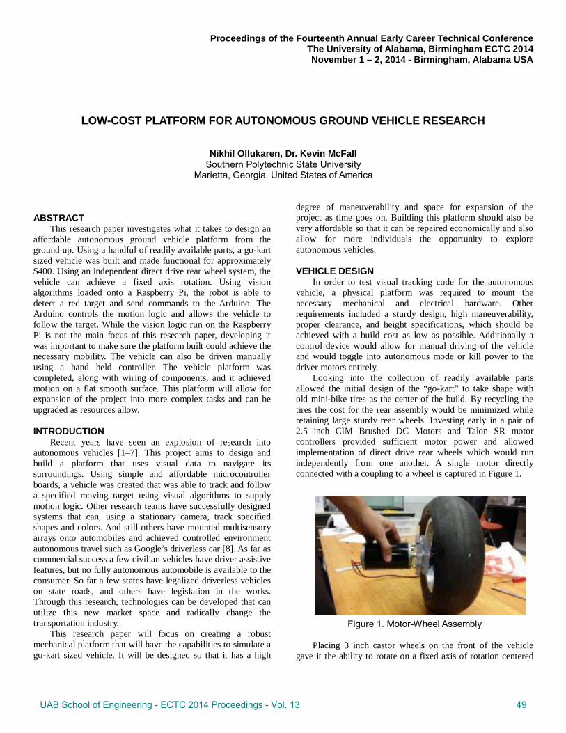
Looking into the collection of readily available parts allowed the initial design of the “go-kart” to take shape with old mini-bike tires as the center of the build. By recycling the tires the cost for the rear assembly would be minimized while retaining large sturdy rear wheels. Investing early in a pair of 2.5 inch CIM Brushed DC Motors and Talon SR motor controllers provided sufficient motor power and allowed implementation of direct drive rear wheels which would run independently from one another. A single motor directly connected with a coupling to a wheel is captured in Figure 1.

Figure 1. Motor-Wheel Assembly

Placing 3 inch castor wheels on the front of the vehicle

gave it the ability to rotate on a fixed axis of rotation centered


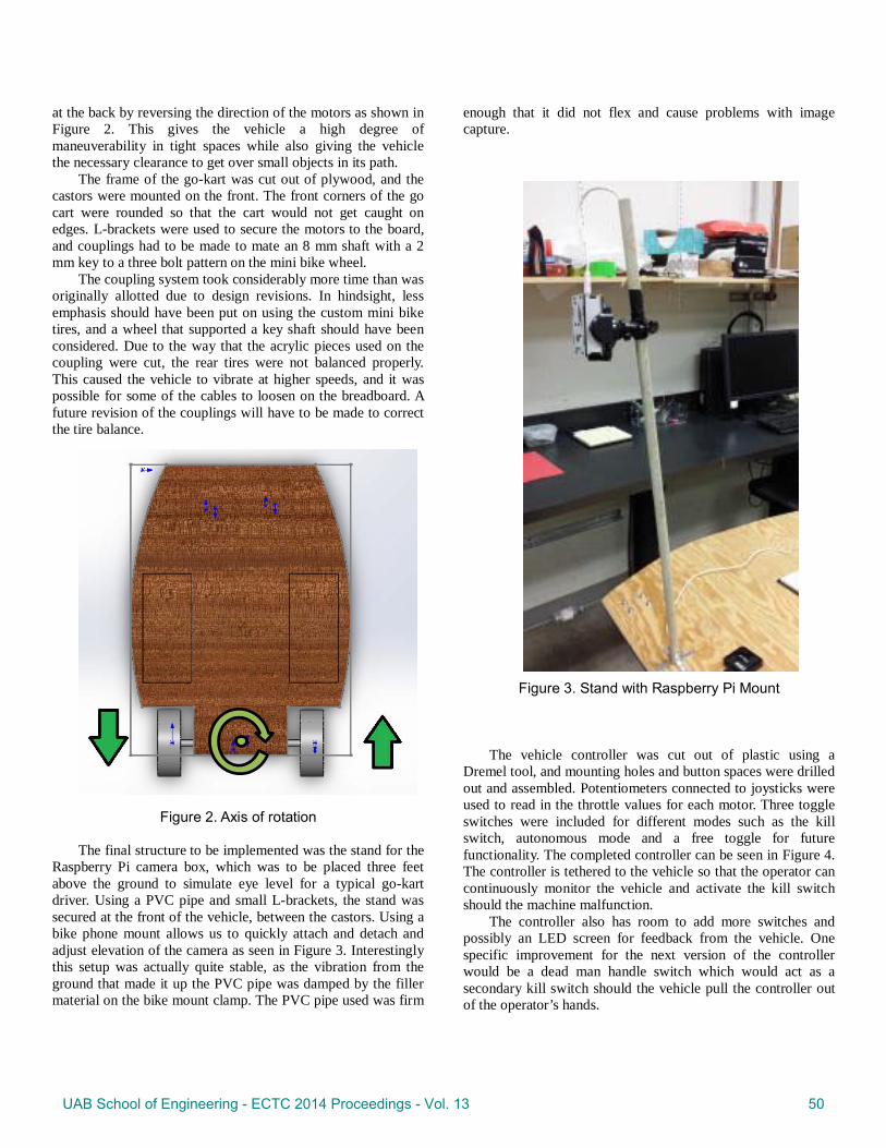
at the back by reversing the direction of the motors as shown in Figure 2. This gives the vehicle a high degree of maneuverability in tight spaces while also giving the vehicle the necessary clearance to get over small objects in its path.

The frame of the go-kart was cut out of plywood, and the castors were mounted on the front. The front corners of the go cart were rounded so that the cart would not get caught on edges. L-brackets were used to secure the motors to the board, and couplings had to be made to mate an 8 mm shaft with a 2 mm key to a three bolt pattern on the mini bike wheel.

The coupling system took considerably more time than was originally allotted due to design revisions. In hindsight, less emphasis should have been put on using the custom mini bike tires, and a wheel that supported a key shaft should have been considered. Due to the way that the acrylic pieces used on the coupling were cut, the rear tires were not balanced properly. This caused the vehicle to vibrate at higher speeds, and it was possible for some of the cables to loosen on the breadboard. A future revision of the couplings will have to be made to correct the tire balance.

Figure 2. Axis of rotation

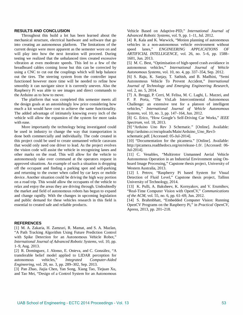
The final structure to be implemented was the stand for the

Raspberry Pi camera box, which was to be placed three feet above the ground to simulate eye level for a typical go-kart driver. Using a PVC pipe and small L-brackets, the stand was secured at the front of the vehicle, between the castors. Using a bike phone mount allows us to quickly attach and detach and adjust elevation of the camera as seen in Figure 3. Interestingly this setup was actually quite stable, as the vibration from the ground that made it up the PVC pipe was damped by the filler material on the bike mount clamp. The PVC pipe used was firm

enough that it did not flex and cause problems with image capture.

Figure 3. Stand with Raspberry Pi Mount

The vehicle controller was cut out of plastic using a

Dremel tool, and mounting holes and button spaces were drilled out and assembled. Potentiometers connected to joysticks were used to read in the throttle values for each motor. Three toggle switches were included for different modes such as the kill switch, autonomous mode and a free toggle for future functionality. The completed controller can be seen in Figure 4. The controller is tethered to the vehicle so that the operator can continuously monitor the vehicle and activate the kill switch should the machine malfunction.

The controller also has room to add more switches and possibly an LED screen for feedback from the vehicle. One specific improvement for the next version of the controller would be a dead man handle switch which would act as a secondary kill switch should the vehicle pull the controller out of the operator’s hands.


Figure 4. Vehicle Controller

The completed platform met all of the design

specifications, starting with being able to emulate the go-kart dimensions and placing the camera at a view point that would emulate the diver’s point of view. The platform needed to be nimble as well, and this was achieved through the castor and tank drive system. The final design requirement was to allow space for the platform to grow. By leaving seven square feet of plywood space available, the second iteration of sensors will have more than enough space to be mounted. By recycling older components into the design, we were able to keep assembly costs under $400 for the entire build. Figure 5 shows the completed platform with all of the components wired.

MICROCONTROLLER PROGRAMMING While versatile and simple to use, microcontrollers like the

Arduino and applications processors like the Raspberry Pi are limited in their processing speed, especially if parallel processing threads are required. For this reason, an Arduino Uno was chosen to send pulse width modulation (PWM) signals to the motor controllers and the Raspberry Pi for processing the camera image in order to compartmentalize the computing tasks. The Pi was chosen for its camera module, which connects directly to the board with a dedicated camera port. Both the Pi and camera are protected by placing them in a commercially available enclosure.

The Pi collects visual information from the camera, processes it, and sends serial data commands to the Arduino via USB cable as illustrated in Figure 6. The role of the Arduino is to read inputs from the controller and Pi, and write appropriate PWM commands to the motor controllers as described in Figure 7. The PWM signals to the Talon motor controllers consist of 1 to 2 ms pulses periodically with a 20 ms period. Full counter-clockwise motion is achieved with a 1 ms pulse, where 1.5 ms is neutral and 2 ms full clockwise rotation. The software limits PWM output between 1.1 and 1.8 ms in order to operate the tethered vehicle at reasonable speeds.

Figure 5. Completed Vehicle Powering both the Arduino and Pi with a single battery was

more complicated than anticipated. Most desirable would be to power the Arduino with a battery and subsequently the Pi via the USB serial connection; attaching a battery to the vehicle chassis along with the Arduino is simpler than adding one to the Pi mounted on a post. Constructing a supply for the Arduino from a 9 V battery, battery snap, and 2.1 mm power plug is straightforward, and takes advantage of the built-in voltage regulator on the Arduino. However, a diode in the Arduino circuitry [9] allows powering the Arduino via USB but prevents it from supplying power to USB connected devices. As a workaround, a USB cable was modified, with its power wire connected to the 5 V output on the Arduino rather than to the USB connector. Power was supplied to the Pi, although none of the USB ports would activate, not even serial communication across the cable powering it from the Arduino. The final design places a battery pack with the Pi instead, which powers the Arduino via a standard USB cable. A Bytech portable battery charger was used to deliver the requisite 5 V to the Pi, which has no internal voltage regulator and therefore should not be powered directly with batteries. The overall system schematic of how all the components are connected is presented in Figure 8. The source code for the Python script running on the Pi and the Arduino sketch appear in Appendix A and B, respectively.


Figure 6. Flow chart for Raspberry Pi programming.

Figure 7. Flow chart for Arduino programming.

IMAGE PROCESSING The eventual goal of this project is to equip the

autonomous vehicle with sophisticated image processing

algorithms to offer obstacle avoidance and detection of road boundaries for steering control. As a proof of concept, the prototype is programmed to detect and follow a sheet of red paper. The picamera Python library [10] can acquire images at 30 frames per second (FPS), but the overhead of processing the image generally reduces the rate to 2-5 FPS [11], [12]. But the simple code tested using capture_continuous yielded only approximately 1 FPS, which is sufficient for a prototype but obviously must be improved upon for a relevant autonomous vehicle.

The OpenCV computer vision library [13], [14] is used to encode the raw image input into a useful matrix in order to create a binary image true for pixels with red components over 68% and with blue and green components under 47%. A non-zero command is sent via USB to the Arduino if the number of true pixels in the binary image exceeds a particular threshold. The value sent is proportional to the average horizontal position of the true pixels with 1 corresponding to the left side, 64 to middle, and 127 to the right side. Engaging the kill switch on the controller prevents the vehicle from following spurious red objects in the background.

Figure 8. System schematic

The image acquisition and processing script is run

automatically in the background (using the & tag) during startup by executing it in the /etc/rc.local file just before the exit command.

Arduino

Talon SR Talon SR

CIM Motors CIM Motors

Raspberry Pi

DO6 DO9

Portable Battery

USB

USB

12 V Battery

Controller

Read value from kill switch

Kill? Yes

No

Read value from mode switch

Read values from potentiometers

Write PWM proportional to potentiometer values

No Manual?

Value = 1?

Yes

Yes

Write PWM: value = 2 left

turn, 64 straight, 127 right turn

No

Read value from Pi between 1 and 128

Acquire image

Process image

Send value between

0 and 127 to Arduino


RESULTS AND CONCLUSION Throughout this build a lot has been learned about the

mechanical structure, electrical hardware and software that go into creating an autonomous platform. The limitations of the current design were more apparent as the semester wore on and will play into how the next iteration will proceed. During testing we realized that the unbalanced tires created excessive vibration at even moderate speeds. This led to a few of the breadboard cables coming loose but this can be corrected by using a CNC to cut out the couplings which will help balance out the tires. The steering system from the controller input functioned however more time will be needed to refine how smoothly it can navigate since it is currently uneven. Also the Raspberry Pi was able to see images and direct commands to the Arduino as to how to move.

The platform that was completed this semester meets all the design goals at an astonishingly low price considering how much a kit would have cost to achieve the same functionality. The added advantage of intimately knowing every inch of the vehicle will allow the expansion of the system for more tasks with ease.

More importantly the technology being investigated could be used in industry to change the way that transportation is done both commercially and individually. The code created in this project could be used to create unmanned vehicle caravans that would only need one driver to lead. As the project evolves the vision code will assist the vehicle in recognizing lanes and other marks on the road. This will allow for the vehicle to autonomously take over command at the operators request in approved situations. An example of such a situation is dropping off the occupant and finding a parking spot and self-parking and returning to the owner when called by car keys or mobile device. Another situation could be driving the high way portion on a road trip. This would allow the occupants of the vehicle to relax and enjoy the areas they are driving through. Undoubtedly the market and field of autonomous robots has begun to expand and change rapidly. With the changes in upcoming legislation and public demand for these vehicles research in this field is essential to created safe and reliable products.

REFERENCES [1] M. A. Zakaria, H. Zamzuri, R. Mamat, and S. A. Mazlan, “A Path Tracking Algorithm Using Future Prediction Control with Spike Detection for an Autonomous Vehicle Robot,” International Journal of Advanced Robotic Systems, vol. 10, pp. 1–9, Aug. 2013. [2] R. Domínguez, J. Alonso, E. Onieva, and C. González, “A transferable belief model applied to LIDAR perception for autonomous vehicles,” Integrated Computer-Aided Engineering, vol. 20, no. 3, pp. 289–302, Sep. 2013. [3] Pan Zhao, Jiajia Chen, Yan Song, Xiang Tao, Tiejuan Xu, and Tao Mei, “Design of a Control System for an Autonomous

Vehicle Based on Adaptive-PID,” International Journal of Advanced Robotic Systems, vol. 9, pp. 1–11, Jul. 2012. [4] R. Kala and K. Warwick, “Motion planning of autonomous vehicles in a non-autonomous vehicle environment without speed lanes,” ENGINEERING APPLICATIONS OF ARTIFICIAL INTELLIGENCE, vol. 26, no. 5–6, pp. 1588–1601, Jun. 2013. [5] M. C. Best, “Optimisation of high-speed crash avoidance in autonomous vehicles,” International Journal of Vehicle Autonomous Systems, vol. 10, no. 4, pp. 337–354, Sep. 2012. [6] S. Raju, K. Sanjay, T. Sathish, and B. Madhini, “Semi Autonomous Vehicle To Prevent Accident,” International Journal of Technology and Emerging Engineering Research, vol. 2, no. 5, 2014. [7] A. Broggi, P. Cerri, M. Felisa, M. C. Laghi, L. Mazzei, and P. P. Porta, “The VisLab Intercontinental Autonomous Challenge: an extensive test for a platoon of intelligent vehicles,” International Journal of Vehicle Autonomous Systems, vol. 10, no. 3, pp. 147–164, Jun. 2012. [8] G. Erico, “How Google’s Self-Driving Car Works,” IEEE Spectrum, vol. 18, 2013. [9] “Arduino Uno Rev 3 Schematic.” [Online]. Available: http://arduino.cc/en/uploads/Main/Arduino_Uno_Rev3-schematic.pdf. [Accessed: 05-Jul-2014]. [10] “Documentation for the picamera.” [Online]. Available: http://picamera.readthedocs.org/en/release-1.0/. [Accessed: 06-Jul-2014]. [11] C. Venables, “Multirotor Unmanned Aerial Vehicle Autonomous Operation in an Industrial Environment using On-board Image Processing,” Capstone thesis project, University of Western Australia, 2013. [12] I. Petrov, “Raspberry Pi based System for Visual Detection of Fluid Level,” Capstone thesis project, Tallinn University of Technology, 2014. [13] K. Pulli, A. Baksheev, K. Kornyakov, and V. Erumihov, “Real-Time Computer Vision with OpenCV,” Communications of the ACM, vol. 55, no. 6, pp. 61–69, Jun. 2012. [14] S. Brahmbhatt, “Embedded Computer Vision: Running OpenCV Programs on the Raspberry Pi,” in Practical OpenCV, Apress, 2013, pp. 201–218.


APPENDIX A – RASPBERRY PI PYTHON SCRIPT import io import cv2 import numpy as np from serial import Serial rowRes = 60 colRes = 80 ser = Serial('/dev/ttyACM0') with picamera.PiCamera() as camera: camera.resolution = (colRes, rowRes) camera.framerate = 30 stream = io.BytesIO() for foo in camera.capture_continuous (stream, format='jpeg'): stream.truncate() stream.seek(0) data = np.fromstring (stream.getvalue(), dtype=np.uint8) im = cv2.imdecode(data,1) B = im[:,:,0] // Blue G = im[:,:,1] // Green R = im[:,:,2] // Red ind = (R>175) & (B<120) & (G<120) x = 0 count = 0 for row in range(0,rowRes): for col in range(0,colRes) if(ind[row,col] == True): x += col count += 1 x = x/(count+1) // Avoid divide 0 cover=float(count)/rowRes/colRes*100 scale = int(float(x+1)/colrRes*128) if(cover > 0.2): ser.write(str(unichr(scale else:

ser.write(str(unichr(1)))

APPENDIX B – ARDUINO SKETCH #define baseSpeed 200 #define maxSpeed 400 int val = 1; int newVal, time, buffer; int right, left; void setup() { pinMode(6, OUTPUT); // Left motor pinMode(9, OUTPUT); // Right motor pinMode(5, INPUT); // Mode switch pinMode(4, INPUT); // Kill switch Serial.begin(9600); } void loop() { if(digitalRead(4) == LOW) {

if(digitalRead(5) == LOW) { newVal = 0; while((buffer=Serial.read())>=0) newVal = buffer; if(newVal > 0) val = newVal; if(val == 1) { digitalWrite(6,HIGH); delayMicroseconds(1500); digitalWrite(6,LOW); delayMicroseconds(20000-1500); } else { if(val < 64) { // Move left time = map(val,64,0, baseSpeed,maxSpeed); digitalWrite(6,HIGH); digitalWrite(9,HIGH); delayMicroseconds(1500-

baseSpeed); digitalWrite(6,LOW); delayMicroseconds(baseSpeed + time); digitalWrite(9,LOW); delayMicroseconds(20000 – 1500 - time); } else { // Move right time = map(val, 64, 128, 0, maxSpeed-baseSpeed); digitalWrite(6,HIGH); digitalWrite(9,HIGH delayMicroseconds(1500-time); digitalWrite(6,LOW); delayMicroseconds(time + baseSpeed); digitalWrite(9,LOW); delayMicroseconds(20000 – 1500 - time); } } } else { // Manual mode left = map(analogRead(1),0,1023, 1500,1500+maxSpeed); right = map(analogRead(2),0,1023, 1500,1500+maxSpeed); digitalWrite(6,HIGH); digitalWrite(9,HIGH); delayMicroseconds(1500 - left); digitalWrite(6,LOW); delayMicroseconds(left + right); digitalWrite(9,LOW); delayMicroseconds(20000 - 1500 – right); } } }



LASER SCANNING VIBROMETER FOR REMOTE PROCESS PERFORMANCE MONITORING OF AUTOMATED MANUFACTURING OPERATIONS

Hadi Fekrmandi David Meiller

Florida International University Miami, Florida, USA

Ibrahim Nur Tansel Florida International University

Miami, Florida, USA

Abdullah Alrashidi

University of Miami Miami, Florida, USA

ABSTRACT In this study the Surface Response to Excitation method

(SURE) is employed for remote performance monitoring of manufacturing operations. Basic manufacturing operations including cutting and drilling are studied and the ability of the method to evaluate the dimensional accuracy of each process is investigated.

The SURE method uses piezoelectric elements to monitor the changes to the condition of structure. One of the piezo elements excites the high frequency surface guided waves and the second piezo senses the received waves in another point. In this study, a laser-scanning vibrometer (LSV) is used to measure surface vibrations. The advantage of LSV over the piezo sensor is that the measurements are not limited to a certain point, and LSV can scan surface vibrations from any point on the surface of the structure. Each operation was performed in a certain number of steps and during each step laser scanning LSV made measurements from the predetermined scan-points on a grid.

The normalized sums of square differences (NSSDs) of the frequency spectrums in every step of the operations are calculated using the SURE algorithm. Results revealed that the NSSD values increase at each step of operation. Therefore, dimensional accuracy of the work piece could be related to NSSD values to monitor the quality of the performance of process. This behavior was observed not only in scan points adjacent to the position of operation, but also it was observed to some extent in all of the scan points. Also the contour map plots of NSSD values clearly demonstrated the creation and development of the operation in the correct position.

The proposed method has an advantage over conventional vision-based process performance monitoring systems. By choosing the scan points away from the position of operation, it is possible to monitor the procedure without the need to interrupt the operation for cleaning the work piece. The reliability of this technique is examined through observation of similar results after repeating the experimentation in similar conditions.

INTRODUCTION Automation is essential for manufacturing products with

reasonable cost. During automated manufacturing, the quality of the manufacturing process should be monitored. Many methods have been developed to evaluate the manufacturing operation; however, the complexity and the cost of these systems limit their implementation in industry. The purpose of this study was to develop a new structural health monitoring method for condition monitoring of the quality of the machining operations.

The structural health monitoring (SHM) community has developed methods for the evaluation of the integrity of structures, which resulted in improvement of reliability and decrease in periodical maintenances. More recently, active structural health monitoring methods have received a lot of attention. These methods detect structural defects via exciting the surface of the structure and monitoring its response at another point. The major trends in the active health monitoring techniques could be divided into two main categories: the lamb wave based methods [1,2] or impedance based (EMI) methods [3,4

In the surface guided waves (lamb wave) based methods, structural problems are detected from monitoring the reflections of high frequency emitted signals. The changes of the characteristics of the received signals are processed through time-frequency techniques [

].

5]. However, in the electro-mechanical impedance-based approaches [6], the variation in the impedance of a piezoelectric element attached to the surface of the structure is a criterion to detect structural damage. Experimental studies have shown that the impedance characteristics of a structure are subjected to considerable changes when the structure is exposed to defects with different sizes and types. It has been shown that the impedance-based methods are more sensitive to loading status of structures compared to lamb wave based methods [7

The capabilities of the commercially available automated manufacturing systems are limited to vision-based systems. Due to bulkiness of equipment and expensive costs involved in their processes and some limitations, the commercial

].


implementation of those methods is pending more research and development. Surface Response to Excitation or the SURE Method [7F8], is a structural health monitoring technique that uses two or more piezoelectric sensors on the part’s surface. One of these sensors excites the part at a certain frequency range and creates surface waves. These waves propagate on the surface of the structure. The other piezoelectric element(s) receive the waves initiated from the first piezo. For large and remote access to structures, it is not practical to attach numerous piezoelectric elements in order to get data. For this reason, a laser vibrometer was used as an alternative non-contact data acquisition sensor to gather data via a pre-defined set of scanning points on the structure in SHM applications [ 8F9]. The feasibility of the SURE approach for machining condition monitoring was shown through detecting the modifications to the work-piece, including cuts, holes and welding. However, the reliability of the method was not studied. Also in the past, the data acquisition was limited to the location of attached sensors.

In this study, the scanning laser vibrometer (SLV) was used to evaluate the surface response characteristics at a set of measurement points using the SURE method. Previously, researchers have used the laser vibrometers for health monitoring purposes by evaluating the modal parameters [9F10], strain energy [ 10F11] and the lamb waves [ 11F12] to evaluate the integrity of structures. The guided lamb wave method was also successfully implemented via the SLV to detect fatigue cracks. Bolted joints like gas pipelines and composite structures have been reported to be monitored using EMI based techniques compared to guided lamb wave based methods [ 12F13]. Various sensors, measured signals and signal processing techniques have been used for tool condition monitoring [ 13F14]. Tansel et al. [ 14F15] studied the feasibility of surface guided based techniques for tool condition monitoring. They indicated that the tool wear could be measured accurately with these methods; however, in their method, the tool needs to stop in order to be monitored. Also, surface scratches due to chips could be a resource of variations in measurements.

The objective of this study is to develop a new machining condition monitoring method based on the available structural health monitoring techniques adapted to the application at automated manufacturing processes. We pursued the developments in structural health monitoring techniques within the data acquisition, implementation and signal processing techniques to accomplish a reliable manufacturing process monitoring method. Basic metal cutting processes were considered for this study, including drilling, cutting and assembling.

SURE METHOD THEORY Tansel et al. [ 15F16] developed the surface response to the

excitation (SURE) method. This method requires much simpler and cheaper experimental setup compared to the EMI method. The SURE method uses a piezoelectric element to excite the surface through a certain frequency range, and the surface response is measured with another piezoelectric element sensor

or non-contact laser scanning vibrometer. Like the impedance method, the SURE method calculates the Sum of the Squared Differences (SSD’s) of the magnitude of the transfer function with respect to a reference measurement. It evaluates the estate of health of structure versus its reference status by monitoring these values.

The reference scan is captured before any machining operation on work piece. Then, after each step of operation, another scan is captured. Due to the presence of the operation on the work-piece, its surface response to excitation changes. To quantify this change, the Normalized Sum of the Squared Differences (NSSDs) method is used. First, square differences of scan data versus reference scan is calculated.

[𝐃]𝑚×𝑛 = ‖[𝐀]𝑚×𝑛 − [𝐑]𝑚×𝑛‖2 (1)

(1) R and A are the reference and secondary (altered) data

matrices obtained by the spectrum analyzer. The dimension of these matrices is m rows by n columns. m is the number of scan points and n depends on the sampling frequency of data acquisition system. Therefore each data matrices includes the m number of frequency spectrums, where each of them is distributed over the n frequencies. Sum of square differences (SSD) could be calculated from the following equation:

[𝐒]1×𝑛 = ∑ [𝐃]𝑚×𝑛 (2) The Normalized Squared Differences (NSSDs) are also

obtained by averaging the squared differences values. Dividing SSD matrix with its average value does this:

[𝐃]��𝑚×𝑛 = 1

𝑎𝑣𝑔[𝐃]𝑚×𝑛 (3)

Figure 1 shows the SSD values calculated for spectra of a

scan point on two successive measurements. In the first case on the left, the spectrum of the point is compared to the reference value before anything changes in the condition of structure. In the second case, the spectrum of the point on the grid is compared to the reference value after a load was applied on the structure.

The SSD value in Figure 1 was for a single scan point on the beam. The SURE algorithm calculates the SSD values for the entire scan region. In our study, the change in condition of the structure was the cut and drill hole, and we examined the possibility of using the SURE method to monitor the condition of the operation and possibly evaluate the state of the progress of manufacturing operation.

EXPERIMENTAL TEST SET UP The specimen that was used in this experimentation was a

2in×36in×1/16in aluminum beam. An APC piezoelectric element model D-.750"-2MHz-850 WFB was attached to the middle of the beam using the LOCTITE Hysol Product E-30CL epoxy adhesive. The aluminum beam was clamped in both ends


within a wood frame. This wood frame and beam were fixed to the experiment table to avoid any movements during the operations. This way the scan points remained the same at all steps of the operation. Figure 3 shows the beam, piezo element and frame.

Figure 1 The change of squares of the differences

(SSD’s) in drilling operation.

Figure 2 aluminum beam with a piezoelectric attached in

the middle of it and fixed within the wood frame In this study, a laser scanning Doppler vibrometer (LSV),

model Polytech PSV-400, measured the surface vibrations from a grid of scan points on the aluminum beam. The laser vibrometer includes the scanning head and control system. The junction box of the laser vibrometer has a built-in function generator. During the tests, the function generator constantly generated sweep sign waves with a maximum amplitude of 5V within the 20-40 kHz. Due to the electro-mechanical property of PZT material and the boding between the piezo and beam

surface, the surface guided waves were excited on the beam surface through the piezo element. The frequency range was limited to maximum of 40 kHz according to the maximum sampling ratio of laser vibrometer analogue to digital convertor. A schematic of experimentation procedure is shown in the figure 3.

Figure 3 schematic of experimentation process

As shown in Figure 4, the scan grid includes 42 scan points that are arranged in 3 rows and 14 columns with the piezo element at the middle. The scan points were evenly distributed on both sides of the piezo and the scan points on the piezo were disabled. Size of scan area is 1.5in×21in. Scan grid includes two local operation regions where the manufacturing operations were performed. Region 1 (R1) was used for cutting and region 2 (R2) was used for drilling. Scan points were marked on the work piece in order to make sure that at every step scans were exactly were captured from the same points.

At the first step of experimentation, a cutting operation was performed on at region 1 which is 3in left of the beam center. The depths of cut were 0.125 in, 0.250 in and 0.375 in respectively. The second operation was drilling at region 2, which was performed at 6 steps. Table 1 shows the diameter of drill cutter that was used to create the hole on the aluminum beam at every step:

The PSV software of laser is capable of calculating the Fast Fourier Transform (FFT) of measured time data. The entire scan was captured in a single data file and exported for the post processing purpose. In our study, MATLAB was used to program and implement the SURE algorithm. The NSSD values were calculated for all scan points for each step of operation. Contour map graphs of NSSD values were plotted to visualize the behavior of NSSDs and relate them to the manufacturing operation being studied.


Figure 4. 3×14 scan grid with 42 scan points; Region 1

for cutting (R1) and Region 2 (R2) for drilling

Table 1: Drill hole diameters at during a 6 step drilling process

1 2 3 4 5 6 7 8 .09375 .1093 .125 .1562 .1875 .21875 0.1875 0.250

RESULTS Figure 5 shows the contour map of normalized squared

differences for the cutting process. The red region of the contour map graph clearly identifies the cutting process on the upper edge of aluminum beam in the correct location.

Figure 5 The cutting process on the aluminum beam and

the corresponding contour map of normalized sum of squared differences (NSSDs)

The interesting phenomenon about the obtained results is that although the maximum changes in NSSD values are around the cutting edge, other areas of the beam also demonstrate changes in NSSD values to some extent. There is a yellow and orange area on the left of the hot spot in figure 5, while the right of the cutting edge is mostly blue. This means the NSSD values have undergone more changes in the left hand-side of the cutting edge than the right-hand-side. This phenomenon makes sense knowing that the piezoelectric is located at the center of the beam and the cutting region R1 that is located on the left side of the piezo actuator. The piezo element excited the surface waves and they traveled from center to left of the beam. Once the cutting process was performed, the presence of the cutting edge on the path of surface waves caused change in their propagation characteristics to the rest of the beam. This fact was reflected in the NSSD values, and they increased to some extent in the orange and yellow area of the Figure 5.

During the experiments, the NSSDs values of every scan point was increased after every step of the cutting process. This phenomenon is shown at the Figure 6 for a scan point in the red area close to the cutting operation.

Figure 6 Normalized sum of squared differences (NSSDs) of scan point [2,6] at during the cutting

operation The NSSD values showed similar pattern even in the scan

points that were not adjacent to the cutting edge. Authors believe this phenomenon could be used to monitor the performance of the cutting operation in automated manufacturing systems.

Figure 7 shows an example of the NSSDs on the left of the cut edge within the yellow-orange area of figure 5.

Figure 7 Normalized sum of squared differences (NSSDs)

of scan point [1,3] at during the cutting operation


Due to the observation of Figure 6, the NSSD values could be collected away from where the process is happening for the purpose of the process performance monitoring. The importance of this point is that in industrial manufacturing the area close to the cutting process usually is covered with chips and cooling agent and could not be used for the data acquisition purpose. Even in the vision-based systems cleaning and removing the work-piece is the biggest challenge for commercial application.

The drilling process was performed through 8 steps on the region R2 on the beam. Figure 8 shows how the NSSD values successfully identify the correct location of the drill hole. The red area shows that the maximum values of NSSDs are occurred at adjacent to the drill hole. There is also a yellow area on the right side of the red spot. The presence of this area shows that the wave propagation characteristics are changed after waves travel through the drill hole area.

Figure 8 The drilling process on the aluminum beam and

the corresponding contour map of normalized sum of squared differences (NSSDs)

In figure 9 the NSSD values at each step of drilling process

on a scan point within the red area of figure 8 is shown. A similar increasing behavior could be observed compared to the cutting process. The behavior is almost consistent thought the entire experimentation (other than the step 7) and NSSD values almost doubled at the last step. Therefore, they could be correlated to the hole-diameter and be employed in development of drilling process performance monitoring.

The inconsistency that was observed in the step 7 of the drilling process was due to the noise in laser vibrometer measurements. During this study, the scans performed completely automatically. After each step of operations, the LSV automatically scanned the entire grid and it switched from one scan point to another without the any interference. Although this is much more convenient to perform the scans, it leaves the vulnerability to presence of noise in the measurements and could lead to reduced reliability of method.

Figure 9 Normalized sum of squared differences (NSSDs)

of scan point [2.11] at during the drilling operation In order to reduce the size and cost of the proposed

method, an embedded electronic device has been developed in FIU’s mechatronics laboratory [17

]. A budget estimation of this device is presented in Table 2:

Table 2: estimate budget for implementation of SuRE method

Equipment Alternative Embedded Device Price

Function Generator

Digital Data Synthesizer (DDS-60)

$65

Amplifier Integrated Circuit OPAMP $6.62

DAQ system Integrated Circuit DSP $6.54

Laser vibrometer

WFB PZT element $15

Total $93.16

CONCLUSION In this study, we developed an automated process

monitoring of manufacturing processes through modification of an already existing structural health monitoring technique. The authors believe that once an efficient SHM process is developed, it could be implemented with minimal expense and equipment, and it would be possible to inspect several manufacturing processes. The advantages of such a method are non - interference with the manufacturing process and evaluation of tool or product condition with complicated configuration. Development of a non-contact SHM method for the automated manufacturing process monitoring and feasibility of embedded implementation via the SURE based algorithm will considerably reduce maintenance and operation costs of tools and quality control of products. Due to simplicity of the proposed algorithm, the method avoided heavy computational costs and expensive equipment required in methods like machine vision based SHM. Due to the non-contact nature of the laser beam, it was possible to collect data from any point on the work-piece and locate the best possible points to locate the piezoelectric elements.


The method’s implementation in real world automated manufacturing processes requires considerable more experimentation, in order to overcome some of the non-addressed challenges. The piezo location and optimization of the number of exciters and sensors will be an important topic of future studies in this work. Since a single work-piece could go through several different operations during its journey in the production line, more work is required to develop a method in order to be able to detect multiple operations from each other on a single work-piece. Since the method is being developed from a structural health monitoring background, one of the most important parameters that will be subjected to study is the consistency of the monitoring process. The effect of environmental parameters like temperature and humidity and the effect of work piece material also need to be clarified. In this case the laser vibrometer is going to be used as the non-contact sensor, a comprehensive investigation of the effect of the noise in measurements is necessary.

ACKNOWLEDGEMENT The authors acknowledge the FIU Graduate School for

providing support for this research in the form of Dissertation Year Fellowship. Also, authors gratefully acknowledge Army Research Office for funding the shared facilities used in this research at Florida International University (Grant Number 58940-RT-REP). The test pieces were prepared with Richard-Todd Zicarelli’s help at the Engineering Manufacturing Center (EMC) of the Florida International University. His help has been greatly appreciated.

REFERENCES [1] A. Raghavan, and C. E. Cesnik, "Review of guided-wave structural health monitoring. Shock and Vibration Digest," vol. 39(2), pp. 91-116, 2007. [2] Su, Z., Ye, L., & Lu, Y. (2006). Guided Lamb waves for identification of damage in composite structures: A review. Journal of sound and vibration, 295(3), 753-780. [3] W. Yan, and W. Q. Chen "Structural health monitoring using high-frequency electromechanical impedance signatures. Advances in Civil Engineering," 2010. [4] V. G. Annamdas, and M. A. Radhika, "Electromechanical impedance of piezoelectric transducers for monitoring metallic and non-metallic structures: A review of wired, wireless and energy-harvesting methods. Journal of Intelligent Material Systems and Structures," vol. 24(9), pp. 1021-1042, 2013. [5] Su, Z., Ye, L., & Lu, Y. (2006). Guided Lamb waves for identification of damage in composite structures: A review. Journal of sound and vibration, 295(3), 753-780. [6] Park, G., Sohn, H., Farrar, C. R., & Inman, D. J. (2003). Overview of piezoelectric impedance-based health monitoring and path forward. Shock and Vibration Digest, 35(6), 451-464. [7] I. N. Tansel, J. Rojas, and B. Uragun "Localization of problems with Surface Response to Excitation Method. In 6th International Conference on Recent Advances in Space Technologies-RAST2013," April 2013.

[8] Ibrahim N. Tansel, Benjamin L.Grisso , Gurjiwan Singh , Gurjashan Singh, Srikanth Korla , Liming W. Salvino, “Health Monitoring of Aluminum Weldings with the Surface Response to Excitation (SuRE) Approach,” Proceedings of the 8th International Workshop on Structural Health Monitoring 2011. [9] Hadi Fekrmandi, Javier Rojas, Jason Campbell, Ibrahim Nur Tansel, Bulent Kaya, Sezai Taskin, “Surface Response to Excitation Method for Structural Health Monitoring of Multi-Bolt Joints on a Robotic Arm Using a Scanning Laser Vibrometer”, International Journal of Prognostics and Health Management, 2014, Vol 5. [10] Farrar, C. R., Hemez, F. M., Shunk, D. D., Stinemates, D. W., Nadler, B. R., & Czarnecki, J. J. (2004). A review of structural health monitoring literature: 1996-2001 (p. 303). Los Alamos,, New Mexico: Los Alamos National Laboratory. [11] Sharma, V. K. (2009). Laser doppler vibrometer for efficient structural health monitoring. PhD thesis, Georgia Institute of Technology, 2008. [12] Staszewski, W. J., Lee, B. C., Mallet, L., & Scarpa, F. (2004). Structural health monitoring using scanning laser vibrometry: I. Lamb wave sensing. Smart Materials and Structures, 13(2), 251. [13] D. M. Peairs, G. Park, and D. J. Inman, "Improving accessibility of the impedance-based structural health monitoring method. Journal of Intelligent Material Systems and Structures," vol. 15(2), pp. 129-139, 2004. [14] Rehorn, Adam G., Jin Jiang, and Peter E. Orban. "State-of-the-art methods and results in tool condition monitoring: a review." The International Journal of Advanced Manufacturing Technology 26.7-8 (2005): 693-710. [15] Tansel, Ibrahim N., et al. "Wear estimation by testing the elastic behavior of tool surface." International Journal of Machine Tools and Manufacture 51.10 (2011): 745-752. [16] Tansel, I. N., Singh, G., Korla, S., Grisso, B. L., Salvino, L. W., & Uragun, B. (2011, June). Monitoring the integrity of machine assemblies by using surface response to excitation (SuRE) approach. In Recent Advances in Space Technologies (RAST), 2011 5th International Conference on (pp. 64-67). IEEE. [17] Tansel, Ibrahim N., Javier Rojas, Ahmet Yapici, and Balemir Uragun. "Study of the computational efficiency and validity of the surface response to excitation method." In AIAA infoterch and aerospace conference, pp. 19-21. 2012.



VISUAL LANE DETECTION ALGORITHM USING THE PERSPECTIVE TRANSFORM

Dr. Kevin S. McFall and David J. Tran Southern Polytechnic State University

Marietta, GA USA

ABSTRACT This manuscript develops a visual lane detection algorithm

using the Hough transform to detect strong lines in a road image as candidates for lane boundaries. The search space in the Hough transform is reduced by searching for lane boundaries where they were detected in the previous video frame. The perspective transform is applied to determine the position and orientation of candidate lines, which are trusted as true boundaries if the detected lane width falls within a specified tolerance of the actual width. Results from a nearly 8-minute long video of highway driving in rain indicate that lane boundaries are correctly identified in 95% of the images. Detection errors occur primarily during lane changes and poor lighting when entering underpasses. Including data from inertial measurements, location on digital maps, and steering direction would help to reduce or eliminate the instances of incorrectly detected lane location.

INTRODUCTION Within the past decade the development of autonomous

automobiles has grown significantly. Semi-autonomous vehicles are becoming more common in the commercial car industry. Audi, for example is reinventing their vehicles with many semi-autonomous features such as adaptive cruise control, side assist, and lane assist [1]. However, fully autonomous vehicles are still not available to the public. One factor of autonomous vehicles that requires refinement and improvement is the road detection system. The most common detection method is through a vision-based system due to the ability to collect data in a nonintrusive manner [2]. Typically a vision-based system uses a camera to capture footage and a sensor or laser to scan the preceding road area. Several methods are used to approach a vision-based road detection system. One concept analyzes road textures, and segments the road image based on road and non-road regions [3]. A system using visual memory stores guiding images to determine a drivable path for current road images [4]. A detection method for urban areas was proposed to identify curbs by using a Markov chain to detect and link curb points [5]. Issues involving these methods include the lack of precision and reliability when functioning on a variety of roads and the inability to identify lane boundaries on multi-lane roads.

Lane detection can be accomplished using a variety of techniques. One system used color extraction to identify lane markings on roads. However size, shape, and motion was also considered in the detection process in order to differentiate lanes and cars of similar color [6]. A fusion-based method of laser scanners and video footage was developed to locate the drivable region and then detect any necessary lanes on roads [7]. A vision-based system incorporated vehicle localization on a digital map to detect and predict lanes [8]. Another approach develops modeled spatial context information shared by lanes, using an algorithm applied learns to address issues with shadows [9].

This manuscript introduces a lane-detection approach using the perspective transform, including an approximate distance from both the left and right lane boundaries. A detection algorithm is applied by searching for lines with the largest Hough transform value within the detection range where boundary lines are expected. The algorithm then determines whether the lines are to be trusted as the true lane boundaries based on their physical distances as computed from the perspective transform. In order to successfully navigate autonomously, only one line boundary need be trusted at any time as the position of other unknown boundary can be accurately approximated.

PERSPECTIVE TRANSFORM Image generation in cameras follows the central imaging

model in Figure 1 [10] where a camera with focal length f is physically placed at the origin of the XYZ axes. Using similar triangles, a point P in space is projected to position p on the xy image plane according to

and X Yx f y fZ Z

= = (1)

A lane boundary line Z MX B= + (2) with slope M and intercept B in space would be located a distance L to the left of the driver at an angle φ as in Figure 2 where


cot and cscM B Lφ φ= = (3) Assuming all objects to be detected, i.e. lane boundary lines, are located at Y = H where H is the height of the camera above the ground, and substituting Equation (2) into Equation (1), the lane boundary projects to the line

HM Hfy x mx bB B

= − + = + (4)

in the image plane. The detection algorithm supplies the image line parameters m and b which combined with Equation (3) simplify to a lane boundary positioned at

1

2 2 2 and tanH bL

mfb f mφ −= = −

+ (5)

In general, a line in the image plane could correspond to an infinite number of lines in real space, but Equation (5) shows that restricting lines to a horizontal plane distance H below the camera achieves a one-to-one correspondence between lines in the image plane and real space.

Figure 1: Geometry for projecting a point P in XYZ space

to its location p on the xy camera image plane.

The diagonal angle of view ψ is the angle between lines from opposite corners of the image to the XYZ origin. This angle, along with focal length f and image aspect ratio R, define the width of the image as

( )12

2

2 tan

1 1

fw

R

ψ=

+ (6)

Figure 2: Geometry of a lane boundary line in real space for a car travelling at a distance L from the

line directed at an angle φ away from line.

Note that b is measured in length units and can be converted to a pixel position with

pixcN

b bw

= (7)

where Nc is the horizontal pixel resolution. Combining Equations (5)-(7) rewrite the lane boundary position and orientation as

( )

( )

22 21

pix 2

1pix 21

2

and2 tan 1 1

2 tantan

1 1

c

c

HLb N R m

b

mN R

ψ

ψφ −

= + +

= −+

(8)

Locating the lane line boundary in relation to the driver therefore requires the detection algorithm to supply the equation of the line in the image plane via m and bpix, the camera height H, horizontal image resolution Nc, aspect ratio R, and angle of view φ. Note that the angle of view is the only required specification of the camera hardware.

LINE DETECTION USING HOUGH TRANSFORM The strategy for the line detection algorithm is to first

apply a Canny edge filter to create a binary image in which to search for lines. A Hough transform [10] then tallies the number of pixels in the binary image falling on any given line in the image. In order to reduce the complexity of the Hough transform, the top half of the image is cropped out since it falls above the vanishing point for all road boundary lines. Additionally, the left and right lane boundaries will always be located in the left and right sides of the image, respectively. For this reason the bottom left and bottom right quarters of the road image are analyzed separately.

X

Z

L φ

B

M 1

Z

Y

X

y

x

P(X,Y,Z)

p

f


The Hough transform discretizes all possible lines using parameters ρ and θ rather than m and b as illustrated in Figure 4 to avoid discontinuities in the value of slope. The quantity ρ, measured in pixels, represents the perpendicular distance from the line to the top left corner of the image, which is different depending on whether the left or right bottom quarter image is being analyzed as reflected in parts a) and b) of Figure 4. The detection algorithm returns the distance ρ and angle θ of a detected line, which is converted to slope using

tanm θ= (9) and pixel intercept with

1pix 2 tan

sincb N ρ θθ

= − −

(10)

for a line to the left in Figure 4a and

pix cosb ρ

θ= (11)

for a line to the right in Figure 4b.

Figure 4: Defining a line in the image space with either m and b or ρ and θ for the a) lower left quarter image and

the b) lower right quarter image.

Results of the Hough transform appear as an image such as that in Figure 5b where the pixel intensity for a line with any given ρ and θ represents the number of pixels in the binary edge image which fall on the line. The guiding principle for the detection algorithm is to find local maximum in the Hough image in the vicinity of where the lane boundary was identified in the image stream’s previous picture frame. The road scene in Figure 5a produces the Hough image in Figure 5b where the dashed line on the road and circle in the Hough image represent where the lane boundary was in the previous frame. A first estimate for the new lane boundary is determined by finding the maximum Hough value within a limited range bounded by the smallest square area surrounding the circle in Figure 5b. This square area is successively enlarged until both the average and maximum Hough value in the bounded area stop increasing.

The ρ and θ line with the largest Hough value within the final bounded area is selected as a potential lane boundary line. Notice how the two sides of the lane stripe are identified by the detection algorithm, either of which are acceptable, and other strong lines such as the road edge and guardrail are avoided.

Figure 5: Road image a) and corresponding Hough transform b) used in the algorithm for detecting lane

boundaries.

EVALUATING THE ACCURACY OF DETECTED LINES The line detection algorithm described above may fail for

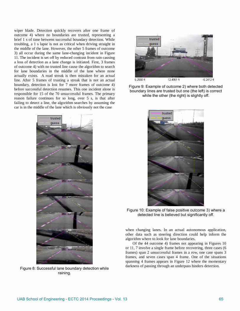
any number of reasons such as poor lighting, occluded camera view, nondescript lane boundary lines, etc. The perspective transformation is used to identify false positives returned by the detection algorithm. The ρ and θ values for the left and right potential lane boundaries are used with Equations (9)-(11) and Equation (8) to determine the distance from and angle each line makes with the camera position. The position of both boundary lines are trusted if the distance between them is within 10% of the known lane width for the road. An example of such a situation appears in Figure 6a where both trusted lane boundaries are marked with solid lines. Also indicated are the

lane position from previous frame

successive lines identified by the detection algorithm

other strong lines in image

a)

b)

ρ (pixels)

θ (rad)

lane position from previous frame successive lines identified by the

detection algorithm

other strong lines in image

boundary of growing region to locate maximum

b) y

–m 1

ρ b

θ x

a) y

–m 1

ρ b

θ x


distances from the camera of both detected lines (left and right), and the difference between them (center) which is a reflection of the detected lane width. If the distance between detected lines is not within tolerance, one of the detected lines may still be trusted according to: • Trust the detected left (or right) line if it was trusted in the

previous frame and its distance L has not changed more than 1/6 of a lane width and the angle φ has not changed more than 5° from the previous frame.

• Trust the closer of the two detected lines if the distance between them is within 10% of the known double lane width (this covers the case where the detection algorithm correctly identifies a two lane span instead of one)

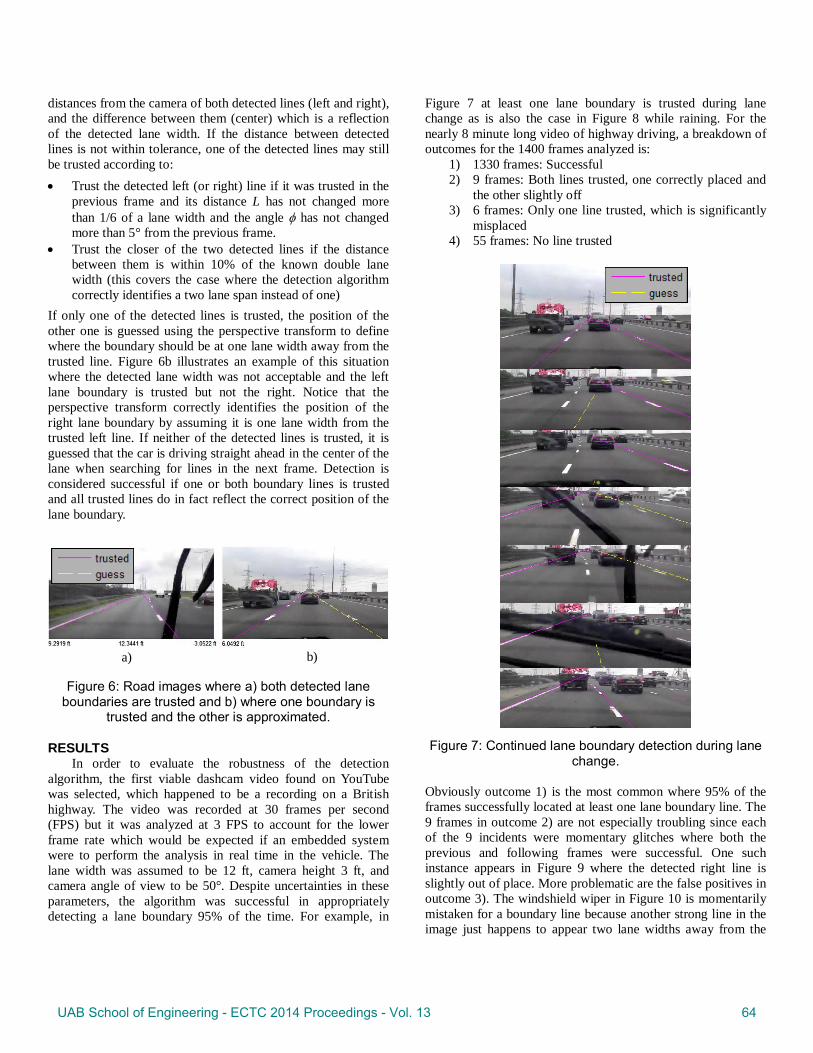
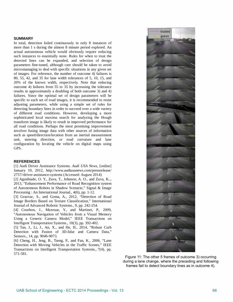
If only one of the detected lines is trusted, the position of the other one is guessed using the perspective transform to define where the boundary should be at one lane width away from the trusted line. Figure 6b illustrates an example of this situation where the detected lane width was not acceptable and the left lane boundary is trusted but not the right. Notice that the perspective transform correctly identifies the position of the right lane boundary by assuming it is one lane width from the trusted left line. If neither of the detected lines is trusted, it is guessed that the car is driving straight ahead in the center of the lane when searching for lines in the next frame. Detection is considered successful if one or both boundary lines is trusted and all trusted lines do in fact reflect the correct position of the lane boundary.

Figure 6: Road images where a) both detected lane boundaries are trusted and b) where one boundary is

trusted and the other is approximated.

RESULTS In order to evaluate the robustness of the detection

algorithm, the first viable dashcam video found on YouTube was selected, which happened to be a recording on a British highway. The video was recorded at 30 frames per second (FPS) but it was analyzed at 3 FPS to account for the lower frame rate which would be expected if an embedded system were to perform the analysis in real time in the vehicle. The lane width was assumed to be 12 ft, camera height 3 ft, and camera angle of view to be 50°. Despite uncertainties in these parameters, the algorithm was successful in appropriately detecting a lane boundary 95% of the time. For example, in

Figure 7 at least one lane boundary is trusted during lane change as is also the case in Figure 8 while raining. For the nearly 8 minute long video of highway driving, a breakdown of outcomes for the 1400 frames analyzed is:

1) 1330 frames: Successful 2) 9 frames: Both lines trusted, one correctly placed and

the other slightly off 3) 6 frames: Only one line trusted, which is significantly

misplaced 4) 55 frames: No line trusted

Figure 7: Continued lane boundary detection during lane

change. Obviously outcome 1) is the most common where 95% of the frames successfully located at least one lane boundary line. The 9 frames in outcome 2) are not especially troubling since each of the 9 incidents were momentary glitches where both the previous and following frames were successful. One such instance appears in Figure 9 where the detected right line is slightly out of place. More problematic are the false positives in outcome 3). The windshield wiper in Figure 10 is momentarily mistaken for a boundary line because another strong line in the image just happens to appear two lane widths away from the

a) b)


wiper blade. Detection quickly recovers after one frame of outcome 4) where no boundaries are trusted, representing a brief 1 s of time between successful boundary detection. While troubling, a 1 s lapse is not as critical when driving straight in the middle of the lane. However, the other 5 frames of outcome 3) all occur during the same lane-changing incident in Figure 11. The incident is set off by reduced contrast from rain causing a loss of detection as a lane change is initiated. First, 3 frames of outcome 4) with no trusted line cause the algorithm to search for lane boundaries in the middle of the lane where none actually exists. A road streak is then mistaken for an actual line. After 5 frames of trusting a streak that is not an actual boundary, detection is lost for 7 more frames of outcome 4) before successful detection resumes. This one incident alone is responsible for 15 of the 70 unsuccessful frames. The primary reason failure continues for so long, over 5 s, is that after failing to detect a line, the algorithm searches by assuming the car is in the middle of the lane which is obviously not the case

Figure 8: Successful lane boundary detection while

raining.

Figure 9: Example of outcome 2) where both detected boundary lines are trusted but one (the left) is correct

while the other (the right) is slightly off.

Figure 10: Example of false positive outcome 3) where a

detected line is believed but significantly off.

when changing lanes. In an actual autonomous application, other data such as steering direction could help inform the algorithm where to look for lane boundaries.

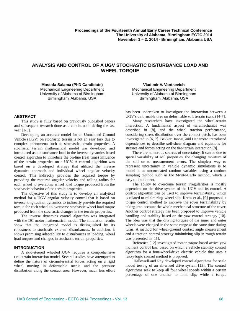
Of the 44 outcome 4) frames not appearing in Figures 10 or 11, 7 involve a single frame before recovering, three cases (6 frames) span 2 unsuccessful frames in a row, one case spans 3 frames, and seven cases span 4 frame. One of the situations spanning 4 frames appears in Figure 12 where the momentary darkness of passing through an underpass hinders detection.


SUMMARY In total, detection failed continuously in only 8 instances of more than 1 s during the almost 8 minute period explored. An actual autonomous vehicle would obviously require reducing such instances to essentially none. Rules for when to trust the detected lines can be expanded, and selection of design parameters fine-tuned, although care should be taken to avoid micromanaging to deal with specific situations in any given set of images. For reference, the number of outcome 4) failures is 80, 55, 42, and 35 for lane width tolerances of 5, 10, 15, and 20% of the known width, respectively. Note that reducing outcome 4) failures from 55 to 35 by increasing the tolerance results in approximately a doubling of both outcome 3) and 4) failures. Since the optimal set of design parameters will be specific to each set of road images, it is recommended to resist adjusting parameters, while using a simple set of rules for detecting boundary lines in order to succeed over a wide variety of different road conditions. However, developing a more sophisticated local maxima search for analyzing the Hough transform image is likely to result in improved performance for all road conditions. Perhaps the most promising improvement involves fusing image data with other sources of information such as speed/direction/location from an inertial measurement unit, steering direction, or road curvature and lane configuration by locating the vehicle on digital maps using GPS.

REFERENCES [1] Audi Driver Assistance Systems. Audi USA News, [online] January 10, 2012, http://www.audiusanews.com/pressrelease/ 2757//driver-assistance-systems (Accessed: August 2014) [2] Agunbiade, O. Y., Zuva, T., Johnson, A. O., and Zuva, K.., 2013, “Enhancement Performance of Road Recognition system of Autonomous Robots in Shadow Scenario,” Signal & Image Processing : An International Journal., 4(6), pp. 1-12. [3] Graovac, S., and Goma, A., 2012, “Detection of Road Image Borders Based on Texture Classification,” International Journal of Advanced Robotic Systems., 9, pp. 242-254. [4] Courbon, J., Mezouar, Y., and Martinet, P., 2009, “Autonomous Navigation of Vehicles from a Visual Memory Using a Generic Camera Model,” IEEE Transactions on Intelligent Transportation Systems., 10(3), pp. 392-402. [5] Tan, J., Li, J., An, X., and He, H., 2014, “Robust Curb Detection with Fusion of 3D-lidar and Camera Data,” Sensors., 14, pp. 9046-9073. [6] Cheng, H., Jeng, B., Tseng, P., and Fan, K., 2006, “Lane Detection with Moving Vehicles in the Traffic Scenes,” IEEE Transactions on Intelligent Transportation Systems., 7(4), pp. 571-581.

Figure 11: The other 5 frames of outcome 3) occurring

during a lane change, where the preceding and following frames fail to detect boundary lines as in outcome 4).


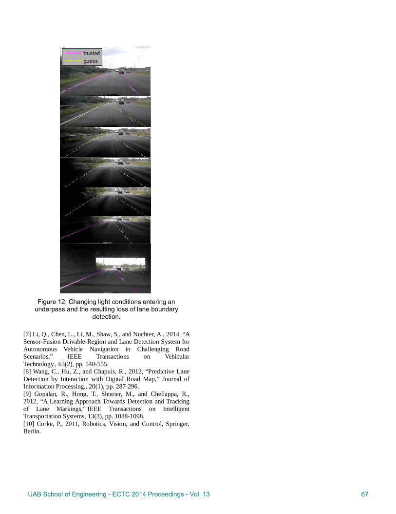
Figure 12: Changing light conditions entering an

underpass and the resulting loss of lane boundary detection.

[7] Li, Q., Chen, L., Li, M., Shaw, S., and Nuchter, A., 2014, “A Sensor-Fusion Drivable-Region and Lane Detection System for Autonomous Vehicle Navigation in Challenging Road Scenarios,” IEEE Transactions on Vehicular Technology., 63(2), pp. 540-555. [8] Wang, C., Hu, Z., and Chapuis, R., 2012, “Predictive Lane Detection by Interaction with Digital Road Map,” Journal of Information Processing., 20(1), pp. 287-296. [9] Gopalan, R., Hong, T., Shneier, M., and Chellappa, R., 2012, “A Learning Approach Towards Detection and Tracking of Lane Markings,” IEEE Transactions on Intelligent Transportation Systems, 13(3), pp. 1088-1098. [10] Corke, P., 2011, Robotics, Vision, and Control, Springer, Berlin.



ANALYSIS AND CONTROL OF A UGV STOCHASTIC DISTURBANCE LOAD AND WHEEL TORQUE

Mostafa Salama (PhD Candidate) Mechanical Engineering Department University of Alabama at Birmingham

Birmingham, Alabama, USA

Vladimir V. Vantsevich Mechanical Engineering Department University of Alabama at Birmingham

Birmingham, Alabama, USA

ABSTRACT This study is fully based on previously published papers

and subsequent research done as a continuation during the last year [1-3].

Developing an accurate model for an Unmanned Ground Vehicle (UGV) on stochastic terrain is not an easy task due to complex phenomena such as stochastic terrain properties. A stochastic terrain mathematical model was developed and introduced as a disturbance load in the inverse dynamics-based control algorithm to introduce the on-line (real time) influence of the terrain properties on a UGV. A control algorithm was based on a developed strategy that utilized the inverse dynamics approach and individual wheel angular velocity control. This indirectly provides the required torque by providing the required angular velocity and rolling radius for each wheel to overcome wheel load torque produced from the stochastic behavior of the terrain properties.

The objective of this study is to develop an analytical method for a UGV angular velocity control that is based on inverse longitudinal dynamics to indirectly provide the required torque for each wheel to overcome stochastic wheel load torque produced from the stochastic changes in the terrain properties.

The inverse dynamics control algorithm was integrated with the DC motor mathematical model. The simulation results show that the integrated model is distinguished by its robustness to stochastic external disturbances. In addition, it shows promising adaptability to disturbances in loading, wheel load torques and changes in stochastic terrain properties.

INTRODUCTION A skid-steered wheeled UGV requires a comprehensive

tire-terrain interaction model. Several studies have attempted to define the nature of circumferential forces acting on a rigid wheel moving in deformable media and the pressure distribution along the contact area. However, much less effort

has been undertaken to investigate the interaction between a UGV’s deformable tires on deformable soft terrain (sand) [4-7].

Many researchers have investigated the wheel-terrain interaction. A fundamental aspect of terramechanics was described in [8], and the wheel traction performance, considering stress distribution over the contact patch, has been investigated in [6, 7]. Bekker, Janosi, and Hanamoto introduced dependences to describe soil-shear diagram and equations for stresses and forces acting on the tire-terrain interaction [8].

There are numerous sources of uncertainty. It can be due to spatial variability of soil properties, the changing moisture of the soil or to measurement errors. The simplest way to represent uncertainty in vehicle dynamic simulations is to model it as uncorrelated random variables using a random sampling method such as the Monte-Carlo method, which is easy to implement.

The ability to overcome terrain irregularities is mostly dependent on the drive system of the UGV and its control. A control algorithm can be used to improve terrainability, which is related to minimizing wheel slip. Krebs et al., [9] proposed a torque control method to improve the rover terrainability by taking into account the whole mechanical structure of the rover. Another control strategy has been proposed to improve vehicle handling and stability based on the yaw control strategy [10]. The idea was that the driving torques of the inner and outer wheels were changed in the same range at the same time during turns. A method for wheel-ground contact angle measurement and a traction control strategy minimizing slip in rough terrain was presented in [11].

Reference [12] investigated motor torque-based active yaw moment control law, based on which a vehicle stability control algorithm for a four-wheel-drive electric vehicle that uses a fuzzy logic control method is proposed.

Hallowell and Ray developed control algorithms for scale model testing of an all-wheel drive system [13]. The control algorithms seek to keep all four wheel speeds within a certain percentage of one another to limit slip, while a torque


distribution system sets the torque command for each wheel, based on its loading and the need to produce a yaw moment [13]. A method for providing optimal torque to each independently driven wheel of a vehicle moving on a slope is given in [14], with a conclusion that the front/rear torque split can be organized proportionally to the ratio of the normal reactions of the wheels.

The UGV is propelled by individual electric motors at each wheel. This enables individual control of each wheel as well as the ability to calculate the rolling radius of each wheel in the driving mode. The vehicle is considered a rigid body, since it does not have a suspension.

A control method for tracking electric ground vehicle planar motion while achieving the optimal energy consumption was presented in [15]. In reference [16], a longitudinal vehicle dynamics controller was designed to control the traction electric motor and reduce the wheel slippage of a front wheel drive vehicle.

It was found by a rigorous theoretical analysis and confirmed in experiments Lefarov and his research group in 1960s and 1970s that the power expended in wheel slippage of a 4x4 drive vehicle is at a minimum at equal slippages of the wheels [17-19].

Wong demonstrated analytically that the slip efficiency is maximized when the slip of the front wheels equals that of the rear wheels. This was done for a 4x4 vehicle subjected to a drawbar load under normal operating conditions; the study was based on a tire-soil interaction research carried out by Reece [20]. Wong et al. showed experimentally that slip efficiency attains its maximum at a theoretical speed ratio equal or close to 1. This means that the slip efficiency reaches its peak when the theoretical velocities of the front and rear wheels are equal to one another [21, 22].

While the majority investigated torque control for each side of the UGV, some focused on individual torque control, which requires measurements of the the torque on each wheel. Also, the rolling radius in the model had not yet been taken into account. The studies referred to were performed for vehicles in steady motion. In addition, controlling UGV wheel angular velocities individually based on the inverse longitudinal dynamics approach was not yet introduced to overcome stochastic terrain disturbances. Thus, a control algorithm is developed based on the inverse dynamics approach, which provides each wheel with both the specified angular velocity and rolling radius to indirectly provide the required wheel torques for a desired input program of motion.

The next section of this study presents key elements of the stochastic tire-terrain interaction that were analyzed based on the Monte Carlo method and integrated with the pneumatic wheel mathematical model. Then, analysis of the rolling resistance in longitudinal motion is presented, as is the generation of the stochastic wheel load torque from the rolling resistance force.

In addition, the UGV mathematical model based on the inverse dynamics approach with the control model will be

introduced. Lastly, the mathematical simulation results will be discussed.

STOCHASTIC TERRAIN PROPERTIES

From the terramechanics approach, which relates the normal and shear stress components, the tire-terrain interaction and how it relates with the wheel forces, it is obvious that the terrain properties 𝑘𝑐 ,𝑘𝜙 ,𝑛, 𝑐,𝜙 and 𝐾 have a direct effect on the calculation of the normal and shear stresses and on circumferential force (thrust) produced in the tire-terrain contact [1].

According to [23], there are numerous sources of uncertainty in a terrain. Uncertainty in geotechnical terrain properties can be formally grouped into Aleatory and Epistemic uncertainty [24]. Aleatory uncertainty represents the natural randomness of a property and, as such, is a function of the spatial variability of the property. Recognizing spatial variability is important because it can help distinguish the distances over which it occurs compared to the scale of the data of interest [25]. Epistemic uncertainty results from a lack of information and shortcomings in measurement and/or calculation.

An extensive literature review was done. Few studies investigated the uncertainty behavior of soil parameters. Madsen [23] showed experimental raw values for nominal soil parameters values from Wong [7] for dry sand with 0% moisture shown in Table 1. It was assumed that spatial variability leads to uncertainty of ±5% about the nominal values [23].

Table 1: Deterministic soil parameters [7] 𝒌𝒄 𝒌𝝓 𝒏 𝒄 𝝓 𝑲

𝒌𝑵/𝒎𝒏+𝟏 𝑘𝑁/𝑚𝑛+2 - 𝑘𝑁/𝑚2 Degrees 𝑚𝑚 0.999 1528.4 1.1 1.04 28 10

According to the literature, it can be said that the soil

parameters can be considered as stochastic variables, where the mean values are the deterministic values shown in Table 1, while the standard deviation, minimum, and maximum were calculated based on the experimental data from [23].

Table 2 shows mean, standard deviation, minimum, and maximum for experimental data in [23].

Table 2: Statistical soft-soil parameters 𝒌𝒄 𝒌𝝓 𝒏 𝒄 𝝓 𝑲

Mean 0.999 1528.4 1.1 1.04 28 10 STD 0.029 44.79 0.032 0.03 0.57 0.001 Min 0.951 1457.6 1.045 0.960 26.58 9.512 Max 1.047 1601.2 1.154 1.115 29.27 10.497 Uncertainties in vehicle dynamic simulations can be

modeled as uncorrelated random variables using random


sampling method such as the Monte Carlo method. This is easy to implement; however, it needs a large number of runs, i.e., 1000.

The Monte Carlo method can be defined as a stochastic simulation that generates random values providing approximate solutions for mathematical problems by performing computational sampling experiments [26]. One of the method’s advantages is the computational efficiency for a high number of parameters, such as complex analytical functions and combinatorial problems, especially relevant for the present work. The Monte Carlo simulation is based on the production of pseudo-random uniformly distributed values, a basic probabilistic distribution, required to simulate all other distributions where the produced numbers must be independent; that is, the number generated in one run does not influence the value of the next one [26].

The efficiency of the stochastic simulation depends on the knowledge about the problem, i.e., the prior information that constrains the simulation; thus the importance of good probability distribution fitting with reliable parameters [27].

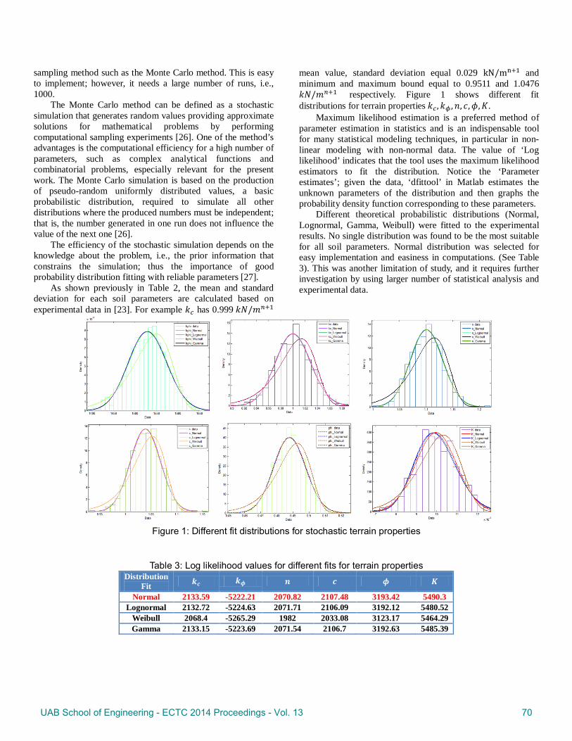
As shown previously in Table 2, the mean and standard deviation for each soil parameters are calculated based on experimental data in [23]. For example 𝑘𝑐 has 0.999 𝑘𝑁/𝑚𝑛+1

mean value, standard deviation equal 0.029 kN/mn+1 and minimum and maximum bound equal to 0.9511 and 1.0476 𝑘𝑁/𝑚𝑛+1 respectively. Figure 1 shows different fit distributions for terrain properties 𝑘𝑐 ,𝑘𝜙 ,𝑛, 𝑐,𝜙,𝐾.

Maximum likelihood estimation is a preferred method of parameter estimation in statistics and is an indispensable tool for many statistical modeling techniques, in particular in non-linear modeling with non-normal data. The value of ‘Log likelihood’ indicates that the tool uses the maximum likelihood estimators to fit the distribution. Notice the ‘Parameter estimates’; given the data, ‘dfittool’ in Matlab estimates the unknown parameters of the distribution and then graphs the probability density function corresponding to these parameters.

Different theoretical probabilistic distributions (Normal, Lognormal, Gamma, Weibull) were fitted to the experimental results. No single distribution was found to be the most suitable for all soil parameters. Normal distribution was selected for easy implementation and easiness in computations. (See Table 3). This was another limitation of study, and it requires further investigation by using larger number of statistical analysis and experimental data.

Figure 1: Different fit distributions for stochastic terrain properties

Table 3: Log likelihood values for different fits for terrain properties Distribution

Fit 𝒌𝒄 𝒌𝝓 𝒏 𝒄 𝝓 𝑲

Normal 2133.59 -5222.21 2070.82 2107.48 3193.42 5490.3 Lognormal 2132.72 -5224.63 2071.71 2106.09 3192.12 5480.52

Weibull 2068.4 -5265.29 1982 2033.08 3123.17 5464.29 Gamma 2133.15 -5223.69 2071.54 2106.7 3192.63 5485.39


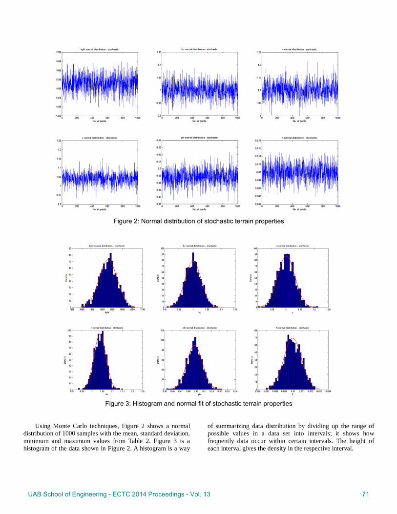
Figure 2: Normal distribution of stochastic terrain properties

Figure 3: Histogram and normal fit of stochastic terrain properties

Using Monte Carlo techniques, Figure 2 shows a normal

distribution of 1000 samples with the mean, standard deviation, minimum and maximum values from Table 2. Figure 3 is a histogram of the data shown in Figure 2. A histogram is a way

of summarizing data distribution by dividing up the range of possible values in a data set into intervals; it shows how frequently data occur within certain intervals. The height of each interval gives the density in the respective interval.


RESISTANCE TO MOTION IN LONGITUDINAL DIRECTION

When moving on uneven, off-road terrain, energy is consumed to overcome the motion resistance. The motion resistance is the sum of several components that occur between the tire and terrain or in the tire itself on a rigid surface. The main components are the soil compaction, rolling resistance (or resistance due to the tire flexing), and bulldozing resistance. Understanding each component is very essential for the UGV dynamics analysis. The main components of the resistance to motion are expressed as [7]

𝑅𝑥 = 𝑅𝑐 + 𝑅𝑏 + 𝑅𝑓 (1)

where 𝑅𝑥 is the total motion resistance force, 𝑅𝑏 is the component due to bulldozing the soil in front of the wheel, 𝑅𝑐 is the component due to soil compaction and 𝑅𝑓 is the component due to the tire flexing [7].

Bekker proposed the following expression to determine the compaction resistance of a soil [28]

𝑅𝑐 = [𝑏(𝑝𝑖+𝑝𝑐)](𝑛+1)/𝑛

�𝑘𝑐+𝑏𝑘𝜙�1𝑛 (𝑛+1)

(2)

where 𝑝𝑖 is the tire inflation pressure and 𝑝𝑐 is the tire carcass stiffness pressure, 𝑏 is the wheel width when it is the smaller dimension of the contact patch. Pressure 𝑝𝑐 is difficult to determine, since it varies with the change of the inflation pressure and normal load of the tire. For this case, Bekker introduced an expression to determine the ground pressure 𝑝𝑔, which is equal to the sum of both inflation pressure and tire carcass stiffness pressure. The latter is normally available in the tire manufacturer documentation for a given inflation pressure and wheel load [8].

Due to the hysteresis of the tire material caused by the flexing of the tire, resisting force 𝑅𝑓 against the motion of the tire appears. Bekker proposed the following semi-empirical relation to predict 𝑅𝑓 based on test data [28]:

𝑅𝑓 = �3.581 𝑏 𝐷2 𝑝𝑔 𝜀 (0.0349𝜃𝑐−sin 2𝜃𝑐)�𝜃𝑐(𝐷−2𝛿𝑡)

(3)

𝜃𝑐 = 𝑐𝑜𝑠−1[(𝐷 − 2𝛿𝑡)/𝐷] is the contact angle in degrees and 𝜀 = 1 − exp (−𝑘𝑒𝛿𝑡/ℎ), while 𝛿𝑡 is the tire deflection, ℎ is the tire section height, the coefficient 𝑘𝑒 is equal to 15 for bias-ply tire and 7 for radial-ply tire [7].

Bulldozing resistance is developed when a substantial soil mass is displaced by a wheel, as shown in Figure 4. The wheel compresses the surface layers of the soil and pushes the compacted soil in front and behind the tire [8].

Bulldozing resistance can be calculated by implementing the theory of bearing capacity of soils subject to various criteria of failure [8]

𝑅𝑏 = � 𝑏 sin(𝛼+𝜙)2 sin 𝛼 cos𝜙

� �2 𝑐 𝐾𝑐 𝑧 + 𝛾 𝐾𝛾𝑧2� + 𝜋𝛾𝑙𝑟3(90−𝜙)540

+𝜋𝑐𝑙𝑟2

180+ 𝑐𝑙𝑟2 tan(45 + 𝜙

2) (4)

where 𝐾𝑐 = (𝑁𝑐 − tan𝜙) cos2 𝜙, 𝐾𝛾 = � 2𝑁𝛾tan𝜙

+ 1� cos2 𝜙,

𝛼 = cos−1(1 − 2𝑧𝐷

), and 𝑙𝑟 = 𝑧 tan2(45− 𝜙2

).

where 𝑧 is the wheel sinkage , 𝛼 is the angle of approach, 𝑙𝑟 is the distance of rupture, 𝑁𝑐 and 𝑁𝛾 are Terzaghi Coefficients [29], 𝐷 is the wheel diameter, and 𝛾 is the soil density.

Figure 4. Bulldozer effect in longitudinal direction

STOCHASTIC DISTURBANCE TORQUE

The disturbance load torque at the motor’s shaft can affect the performance of the motor and the UGV. Taking this disturbance into account enhances the robustness of the system. The disturbance load is generated using stochastic terrain behavior characteristics [1,2].

The wheel load torque can be determined from

𝑇𝑤𝑙𝑖′(′′) = �𝑅𝑥𝑖

′(′′) + 𝐹𝑓𝑟𝑎𝑚𝑒.𝑥𝑖′(′′) + 𝐹𝑗𝑖

′(′′)� 𝑟𝑤0𝑖′(′′) + 𝐼𝑤𝑖

′(′′)𝜀𝑤𝑖′(′′)

(5)

where 𝐼𝑤 is the wheel inertia, 𝜀𝑤 is the wheel angular acceleration and 𝑟𝑤0 is the wheel radius in the driven mode.


𝑅𝑥𝑖′(′′) were calculated from Eqn. (1), which was used in

the terrain blocks in the control algorithm block diagram shown in Fig. 10, which have a stochastic behavior produced from the stochastic terrain.

Figure 5 shows the stochastic load torque to all wheels of the UGV on a horizontal terrain (no longitudinal slopes or terrain irregularities).

Figure 5: Stochastic load torque

UGV INVERSE DYNAMICS AND CONTROL

A free-body diagram of an AWD (All Wheel Drive) UGV within the plain of the road is shown in Fig. 6.

Figure 6: A free-body diagram of an all-wheel drive UGV

in straight motion

Figure 6 gives a free-body diagram of UGV normal and

longitudinal dynamics on a slope. With reference to Figs 6 and 7, the equation of motion with the longitudinal acceleration 𝑎𝑥 of the vehicle is written in inverse dynamics formulation in order to determine the UGV total circumferential force 𝐹𝑥𝛴:

𝐹𝑥𝛴 = ∑ 𝐹𝑥𝑖′(′′)2

𝑖=1 = ∑ 𝑅𝑥𝑖′(′′)2

𝑖=1 + 𝑊𝑎𝑎𝑥𝛿𝑟𝑔

± 𝑊𝑎 𝑠𝑖𝑛 𝜃𝑛 + 𝐷𝑎 (6)

where 𝑅𝑥𝑖 is the total rolling resistance force, 𝑊𝑎 is the UGV weight, and ′ and ′′ superscripts denote for right and left wheels, respectively. 𝛿𝑟 is the mass factor that makes allowance for the inertia of rotating masses of the vehicle. As was shown by an analysis, the small frontal area and low operating speed of the UGV allow the air drag 𝐷𝑎 to be neglected.

Figure 7: Vehicle on grade

Figure 8: Normal tire reactions diagram

The vehicle is considered as a rigid body, since it does not

have a suspension as shown in Figs 7 and 8. Taking moments around contact patch of the front axle,

one can receive

𝑅𝑧2(𝑙2 − 𝑎𝑑2) = 𝑅𝑧1𝑎𝑑1 + 𝑚𝑎𝑎𝑥ℎ + 𝑊𝑎 𝑐𝑜𝑠 𝜃𝑛 𝑙0 +𝑊𝑎 𝑠𝑖𝑛 𝜃𝑛 ℎ (7)

For calculation simplicity it can be assumed that 𝑎𝑑1 =

𝑎𝑑2 = 0 (adi is the shift of the normal reaction due to internal tire friction and friction in road-tire contact patch). See Fig. 7.

When the plane of motion is horizontal, 𝜃𝑛 = 0. In addition, it can be assumed that the bulldozing resistances are acting in the same plane of the contact patch. In this case, Eqn. (7) can be written as


𝑅𝑧2 = 𝑊𝑎𝑙0𝑙2

+ 𝑚𝑎𝑎𝑥ℎ𝑙2

(8)

Taking moments around the contact patch of the rear axle,

the following expression is obtained for the normal tire reaction of the front wheels

𝑅𝑧1 = 𝑊𝑎𝑙2−𝑙0𝑙2

− 𝑚𝑎𝑎𝑥ℎ𝑙2

(9)

As seen in Fig. 8, taking the summation of moments about

left side contact patches

𝑅𝑧′ = 𝑊𝑎2−𝑚𝑎𝑎𝑦

ℎ𝑡𝑏

(10)

And by taking the summation of moments about right side

contact patches

𝑅𝑧′′ = 𝑊𝑎2

+ 𝑚𝑎𝑎𝑦ℎ𝑡𝑏

(11)

The normal loads vary due to three factors, including

weight transfer caused by the acceleration, terrain inclination, and a stochastic micro-profile from uneven terrain. The normal loads on each wheel are derived from summing the moments about the ground contact point of the front tires. The acceleration is specified, since the study utilizes the inverse dynamics approach.

Figure 9 shows the results of computer simulations of a stochastic rolling resistance in steady state motion (longitudinal acceleration of the wheel equal to zero) computed using the method introduced.

Figure 9: Stochastic rolling resistance for a UGV

The UGV control algorithm presented is based on the

wheel inverse dynamics-based control presented in the last section. There are two loops in each wheel control: (i) an internal loop to control the acceleration �̇�𝑤, and (ii) an external loop to control the angular velocity 𝜔𝑤.

The inverse dynamics approach requires a defined program of motion as an input to the simulation model. The developed control algorithm controls the angular velocity of four independent driven wheels by equating the slip of each wheel.

First, the input acceleration profile is integrated to obtain the UGV longitudinal velocity 𝑉𝑥 which is used in conjunction with the wheel rolling radius to calculate the reference angular velocity 𝜔𝑤∗ for each wheel as shown in Figure 3.41.

By substituting in Eqn. (6), the UGV total circumferential force can be calculated for different program of motion, plane inclination, and different terrain properties. This requires summing all circumferential forces for all wheels, equating it with Equation (6) and solving the equation for sδ when all slippages are the same.

In parallel, the Terrain blocks in Fig. 10 contain all equations related to the terrain properties, which are used to generate stochastic terrain characteristics under each wheel independently. Then, the Load blocks calculate stochastic wheel load torques. At the same time, the Wheels blocks have the wheel angular velocity control block diagram. These blocks are used to calculate angular velocities and the required wheel motor torques to overcome stochastic disturbance torques.

Figure 10: Control algorithm block diagram

RESULTS

Once applying a stochastic load, the output wheel angular velocity is no longer able to reach the reference input (specified) angular velocity, (see Fig. 11). It should be emphasized here that this computational test is conducted under the condition where all the wheels are independent from each other, i.e., there is no simulation of mechanical connection


between the wheels and the vehicle frame. In the case when no control is applied, the front wheels have lower angular velocities due to higher rolling resistance. The multi-pass effect has a huge influence on the rolling resistance for the rear tires as shown before in Fig. 5. Therefore, the rotational speed of the rear wheels is higher than that of the front wheels.

Figure11: Stochastic wheel angular velocities

𝝎𝒘𝒊′(′′) without inverse dynamic control

The corresponding wheel torques applied to the four

wheels to overcome stochastic terrain load and provide the angular velocities shown in Fig. 11 are shown in Fig. 12.

Figure 12: Stochastic electric motor torque 𝑻𝒎𝒘𝒊

′(′′) produced to overcome the stochastic wheel load torque

𝑻𝒘𝒍𝒊′(′′) without inverse dynamic control

In order to test the proposed control algorithm for all four

wheels sitting on the same frame and having the same linear velocity 𝑉𝑥, an acceleration profile is generated and used as a required program of UGV motion as shown in Fig. 13.

Figure 13: Specified longitudinal acceleration 𝒂𝒙,𝒎 𝒔𝒆𝒄𝟐⁄

Figure 14 illustrates the specified longitudinal velocity

profile that is obtained through the integration of the acceleration.

Figure 14: Specified longitudinal velocity 𝑽𝒙,𝒎 𝒔𝒆𝒄⁄ Figure 15 confirms that the calculated angular velocities

for each wheel are identical with the required (specified) angular velocity, which means that the control algorithm is working properly with minimal error (not exceeding 0.1%) and is very stable in the UGV normal operating conditions.

Figure 15: Angular velocity 𝝎𝒘𝒊

′(′′),𝑹𝑷𝑴

The corresponding wheels motors torques vary to compensate for uncertainties in the stochastic terrain load as shown in Fig. 16.


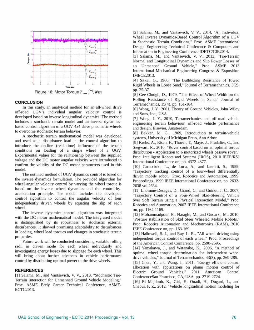
Figure 16: Motor Torque 𝑻𝒎𝒘𝒊

′(′′),𝑵𝒎

CONCLUSION In this study, an analytical method for an all-wheel drive

off-road UGV’s individual angular velocity control is developed based on inverse longitudinal dynamics. The method includes a stochastic terrain model and an inverse dynamics-based control algorithm of a UGV 4x4 drive pneumatic wheels to overcome stochastic terrain behavior.

A stochastic terrain mathematical model was developed and used as a disturbance load in the control algorithm to introduce the on-line (real time) influence of the terrain conditions on loading of a single wheel of a UGV. Experimental values for the relationship between the supplied voltage and the DC motor angular velocity were introduced to confirm the validity of the DC motor parameters used in this model.

The outlined method of UGV dynamics control is based on the inverse dynamics formulation. The provided algorithm for wheel angular velocity control by varying the wheel torque is based on the inverse wheel dynamics and the control-by-acceleration principle. The model includes the developed control algorithm to control the angular velocity of four independently driven wheels by equating the slip of each wheel.

The inverse dynamics control algorithm was integrated with the DC motor mathematical model. The integrated model is distinguished by its robustness to stochastic external disturbances. It showed promising adaptability to disturbances in loading, wheel load torques and changes in stochastic terrain properties.

Future work will be conducted considering variable rolling radii in driven mode for each wheel individually and investigating energy losses due to slippage for each wheel. This will bring about further advances in vehicle performance control by distributing optimal power to the drive wheels.

REFERENCES [1] Salama, M., and Vantsevich, V. V., 2013, "Stochastic Tire-Terrain Interaction for Unmanned Ground Vehicle Modeling," Proc. ASME Early Career Technical Conference, ASME-ECTC2013.

[2] Salama, M., and Vantsevich, V. V., 2014, "An Individual Wheel Inverse Dynamics-Based Control Algorithm of a UGV in Stochastic Terrain Conditions," Proc. ASME International Design Engineering Technical Conference & Computers and Information in Engineering Conference IDETC/CIE2014. [3] Salama, M., and Vantsevich, V. V., 2013, "Tire-Terrain Normal and Longitudinal Dynamics and Slip Power Losses of an Unmanned Ground Vehicle," Proc. ASME 2013 International Mechanical Engineering Congress & Exposition IMECE2013. [4] Sitkei, G., 1966, "The Bulldozing Resistance of Towed Rigid Wheels in Loose Sand," Journal of Terramechanics, 3(2), pp. 25-37. [5] Gee-Clough, D., 1979, "The Effect of Wheel Width on the Rolling Resistance of Rigid Wheels in Sand," Journal of Terramechanics, 15(4), pp. 161-184. [6] Wong, J. Y., 2001, Theory of Ground Vehicles, John Wiley and Sons, Inc., USA. [7] Wong, J. Y., 2010, Terramechanics and off-road vehicle engineering terrain behaviour, off-road vehicle performance and design, Elsevier, Amsterdam. [8] Bekker, M. G., 1969, Introduction to terrain-vehicle systems, University of Michigan Press, Ann Arbor. [9] Krebs, A., Risch, F., Thueer, T., Maye, J., Pradalier, C., and Siegwart, R., 2010, "Rover control based on an optimal torque distribution - Application to 6 motorized wheels passive rover," Proc. Intelligent Robots and Systems (IROS), 2010 IEEE/RSJ International Conference on, pp. 4372-4377. [10] Caracciolo, L., de Luca, A., and Iannitti, S., 1999, "Trajectory tracking control of a four-wheel differentially driven mobile robot," Proc. Robotics and Automation, 1999. Proceedings. 1999 IEEE International Conference on, pp. 2632-2638 vol.2634. [11] Lhomme-Desages, D., Grand, C., and Guinot, J. C., 2007, "Trajectory Control of a Four-Wheel Skid-Steering Vehicle over Soft Terrain using a Physical Interaction Model," Proc. Robotics and Automation, 2007 IEEE International Conference on, pp. 1164-1169. [12] Mohammadpour, E., Naraghi, M., and Gudarzi, M., 2010, "Posture stabilization of Skid Steer Wheeled Mobile Robots," Proc. Robotics Automation and Mechatronics (RAM), 2010 IEEE Conference on, pp. 163-169. [13] Hallowell, S. J., and Ray, L. R., "All wheel driving using independent torque control of each wheel," Proc. Proceedings of the American Control Conference, pp. 2590-2595. [14] Yamakawa, J., and Watanabe, K., 2006, "A method of optimal wheel torque determination for independent wheel drive vehicles," Journal of Terramechanics, 43(3), pp. 269-285. [15] Chen, Y., and Wang, J., 2011, "Energy efficient control allocation with applications on planar motion control of Electric Ground Vehicles," 2011 American Control ConferenceSan Francisco, CA, USA, pp. 2719-2724. [16] El Majdoub, K., Giri, F., Ouadi, H., Dugard, L., and Chaoui, F. Z., 2012, "Vehicle longitudinal motion modeling for


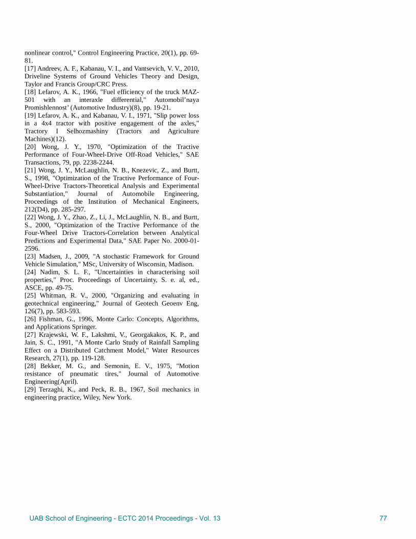
nonlinear control," Control Engineering Practice, 20(1), pp. 69-81. [17] Andreev, A. F., Kabanau, V. I., and Vantsevich, V. V., 2010, Driveline Systems of Ground Vehicles Theory and Design, Taylor and Francis Group/CRC Press. [18] Lefarov, A. K., 1966, "Fuel efficiency of the truck MAZ-501 with an interaxle differential," Automobil’naya Promishlennost’ (Automotive Industry)(8), pp. 19-21. [19] Lefarov, A. K., and Kabanau, V. I., 1971, "Slip power loss in a 4x4 tractor with positive engagement of the axles," Tractory I Selhozmashiny (Tractors and Agriculture Machines)(12). [20] Wong, J. Y., 1970, "Optimization of the Tractive Performance of Four-Wheel-Drive Off-Road Vehicles," SAE Transactions, 79, pp. 2238-2244. [21] Wong, J. Y., McLaughlin, N. B., Knezevic, Z., and Burtt, S., 1998, "Optimization of the Tractive Performance of Four-Wheel-Drive Tractors-Theoretical Analysis and Experimental Substantiation," Journal of Automobile Engineering, Proceedings of the Institution of Mechanical Engineers, 212(D4), pp. 285-297. [22] Wong, J. Y., Zhao, Z., Li, J., McLaughlin, N. B., and Burtt, S., 2000, "Optimization of the Tractive Performance of the Four-Wheel Drive Tractors-Correlation between Analytical Predictions and Experimental Data," SAE Paper No. 2000-01-2596. [23] Madsen, J., 2009, "A stochastic Framework for Ground Vehicle Simulation," MSc, University of Wisconsin, Madison. [24] Nadim, S. L. F., "Uncertainties in characterising soil properties," Proc. Proceedings of Uncertainty, S. e. al, ed., ASCE, pp. 49-75. [25] Whitman, R. V., 2000, "Organizing and evaluating in geotechnical engineering," Journal of Geotech Geoenv Eng, 126(7), pp. 583-593. [26] Fishman, G., 1996, Monte Carlo: Concepts, Algorithms, and Applications Springer. [27] Krajewski, W. F., Lakshmi, V., Georgakakos, K. P., and Jain, S. C., 1991, "A Monte Carlo Study of Rainfall Sampling Effect on a Distributed Catchment Model," Water Resources Research, 27(1), pp. 119-128. [28] Bekker, M. G., and Semonin, E. V., 1975, "Motion resistance of pneumatic tires," Journal of Automotive Engineering(April). [29] Terzaghi, K., and Peck, R. B., 1967, Soil mechanics in engineering practice, Wiley, New York.


uab - ectc 2014 proceedings - section 3 page€¦ · was important to make sure the platform built...

Documents