Circuit Analisys 1

U4. Introduction to passive

filters

Circuit Analysis, 2012-13

Circuit Analisys 2

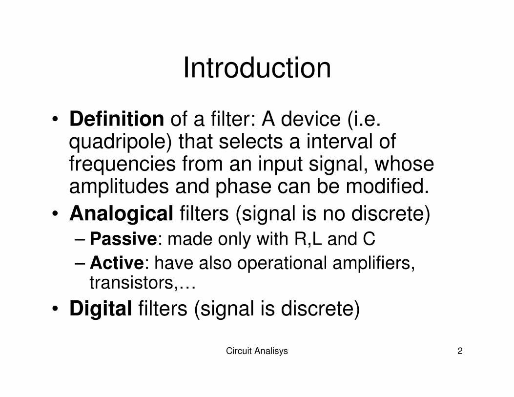
Introduction

• Definition of a filter: A device (i.e. quadripole) that selects a interval of frequencies from an input signal, whose amplitudes and phase can be modified.

• Analogical filters (signal is no discrete)– Passive: made only with R,L and C

– Active: have also operational amplifiers, transistors,…

• Digital filters (signal is discrete)

Circuit Analisys 3

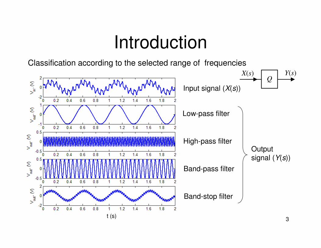
Introduction

X(s) Y(s)Q

t (s)

Input signal (X(s))

Low-pass filter

High-pass filter

Band-pass filter

Band-stop filter

Output

signal (Y(s))

Classification according to the selected range of frequencies

Circuit Analisys 4

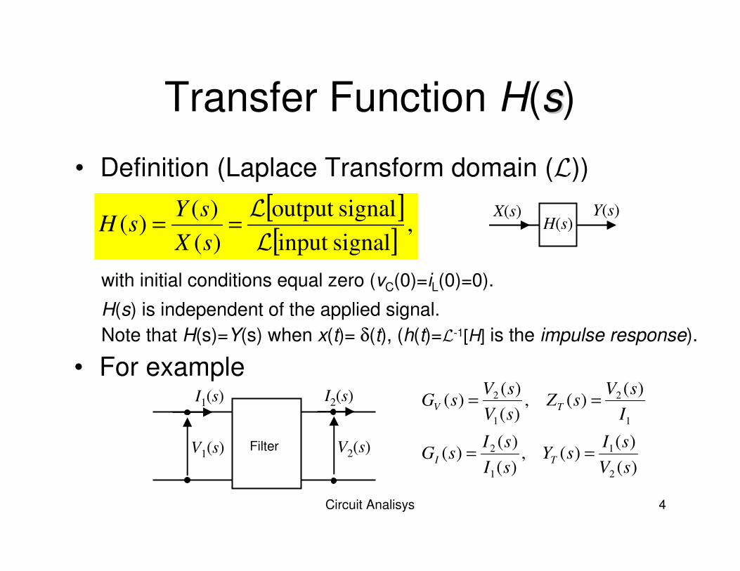
Transfer Function H(ss)

• Definition (Laplace Transform domain (L))

[ ][ ]

,signalinput

signaloutput

)(

)()(

L

L==

sX

sYsH

I1(s) I2(s)

V2(s)V1(s) Filter

)(

)()(,

)(

)()(

)()(,

)(

)()(

2

1

1

2

1

2

1

2

sV

sIsY

sI

sIsG

I

sVsZ

sV

sVsG

TI

TV

==

==

X(s) Y(s)H(s)

with initial conditions equal zero (vC(0)=iL(0)=0).

H(s) is independent of the applied signal.

Note that H(s)=Y(s) when x(t)= δ(t), (h(t)=L-1[H] is the impulse response).

• For example

Circuit Analisys 5

Transfer Function

• Example 1

• Example 2

What kind of filter are they?

Circuit Analisys 6

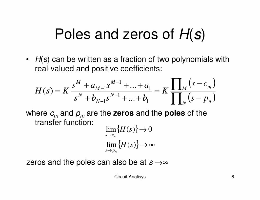
Poles and zeros of H(ss)

• H(s) can be written as a fraction of two polynomials with real-valued and positive coefficients:

( )( )∏

∏−

−=

+++

+++=

−−

−−

N n

M m

N

N

N

M

M

M

ps

csK

bsbs

asasKsH

1

1

1

1

1

1

...

...)(

where cm and pm are the zeros and the poles of the transfer function:

∞→

→

→

→

)(lim

0)(lim

sH

sH

m

m

ps

cs

zeros and the poles can also be at s →∞

Circuit Analisys 7

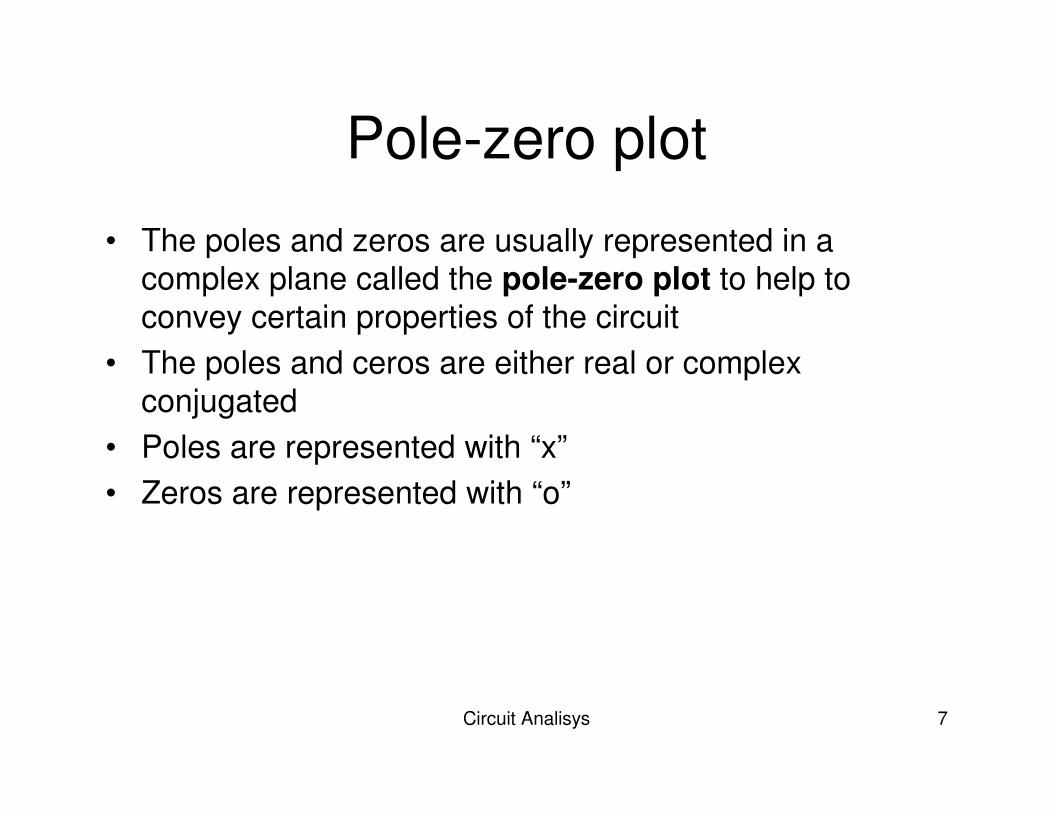
Pole-zero plot

• The poles and zeros are usually represented in a complex plane called the pole-zero plot to help to

convey certain properties of the circuit

• The poles and ceros are either real or complex

conjugated

• Poles are represented with “x”

• Zeros are represented with “o”

Circuit Analisys 8

Frequency response of the

Transfer Function H(ω)

• Frequency response using sinusoidal signals,

then s=jω :( )( )

( ))(jexp)(j

j)( ωφω

ω

ωω H

p

cKH

N n

M m=

−

−=

∏∏

• H(ω) becomes high for ω close to pn

• H(ω) becomes low for ω close to cm

,)](Re[

)](Im[arctan)(

,j

j)(

ω

ωωφ

ω

ωω

H

H

p

cKH

N n

M m

=

−

−=

∏∏

where

is the amplitude response,

is the phase response.

Circuit Analisys 9

Pole-zero plot and |H(ω)|

• Example 3

( )( ),)(

21

1

psps

cssH

−−

−= Poles at s = p1, p2

Zero at s = c1

Poles at s =−1±j5

Zero at s = −5

Poles at s =−1±j10

Zero at s = −5

Poles at s =−5±j10

Zero at s = −5

The closer

the pole to

the imaginary

axis, the

more

pronounced

is the

maximum

Circuit Analisys 10

Pole-zero plot and |H(ω)|

• Example 1

,10

10)(

1

1

+=

+=

sssH

RC

RC

Pole at s= -10

Zero at s→∞

−

+=

+=

10exp

100

10

10

10)(

2

ω

ωωω j

jH

Data: R=1 kΩ, C=100 µF

Circuit Analisys 11

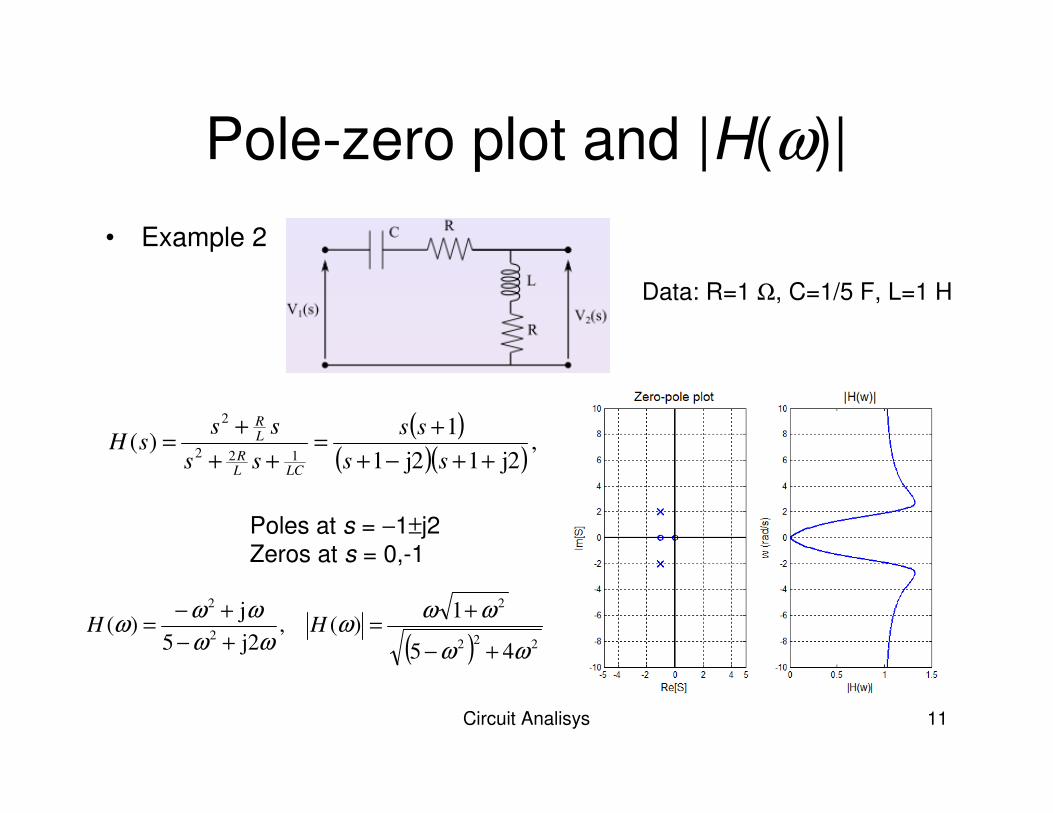
Pole-zero plot and |H(ω)|

• Example 2

( )( )( )

,2j12j1

1)(

122

2

++−+

+=

++

+=

ss

ss

ss

sssH

LCLR

LR

Poles at s = −1±j2Zeros at s = 0,-1

( ) 222

2

2

2

45

1)(,

j25

j)(

ωω

ωωω

ωω

ωωω

+−

+=

+−

+−= HH

Data: R=1 Ω, C=1/5 F, L=1 H

Circuit Analisys 12

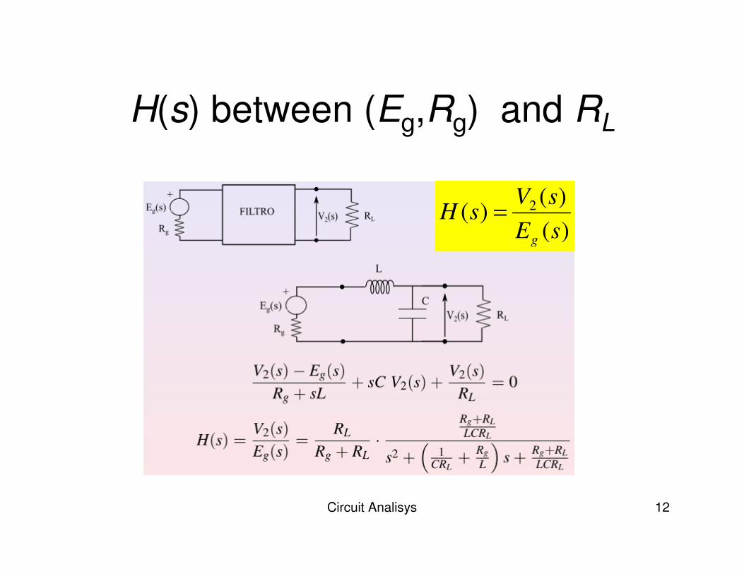
H(s) between (Eg,Rg) and RL

)(

)()( 2

sE

sVsH

g

=

Circuit Analisys 13

Examples of RLC passive filters

• Low-pass filter

– 1st order

– 2nd order

• High-pass filter

– 1rt order

– 2nd order

• Band-pass filter

• Band-stop filter

Circuit Analisys 14

Example: Low-pass filer

Circuit Analisys 15

Example: High-pass filer

Circuit Analisys 16

Example: Band-pass filer

Circuit Analisys 17

Example: Band-stop filter

Circuit Analisys 18

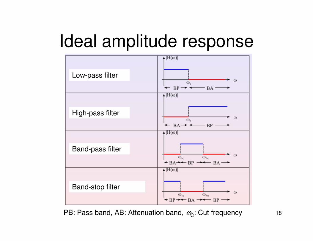
Ideal amplitude response

Low-pass filter

High-pass filter

Band-pass filter

Band-stop filter

PB: Pass band, AB: Attenuation band, ωC: Cut frequency

Circuit Analisys 19

Impulse response of ideal filters

• Ideal filters can not be implemented in practice

• The real filer have to be approached to the ideal filter response using different methods

• The approached filters have not a constant response in the PB and are not entirely zero in the AB

• There exist a transition band between PB and AB

• The order of the filter coincides with the number of poles of H(s)

• The higher the order of the filter the close is his behavior as an ideal filter

• To design filters, layout templates with the tolerance margins are used

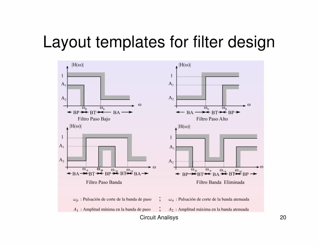
Circuit Analisys 20

Layout templates for filter design

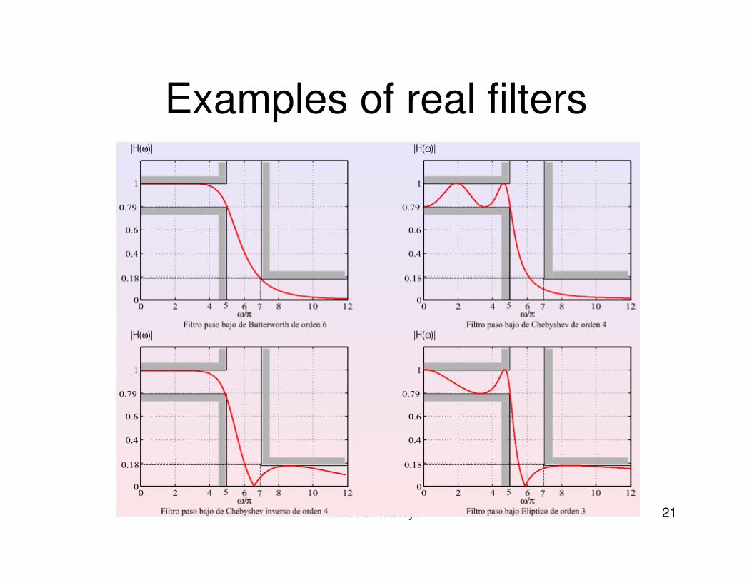
Circuit Analisys 21

Examples of real filters

Circuit Analisys 22

1st order Low-pass filter

• Transfer functionc

c

sksH

ω

ω

+=)(

where ωωωωc is the cut frequency, at this frequency the attenuation of the signal is 3dB:

2

1

)(

)(3

)(

)(log20

maxmax

10 =⇒=−==

ω

ω

ω

ωωωωω

H

H

H

Hcc

22)(

c

ckHωω

ωω

+=

Circuit Analisys 23

Examples 1st order Low-pass filter

• Low-pass RC: • Low-pass RL

L

R

H

c

LR

LR

=

+=

ω

ωω ,

j)(

RC

H

c

RC

RC

1

,j

)(1

1

=

+=

ω

ωω

Circuit Analisys 24

1st order High-pass filter

• Transfer functioncs

sksH

ω+=)(

2

1

)(

)(3

)(

)(log20

maxmax

10 =⇒=−==

ω

ω

ω

ωωωωω

H

H

H

Hcc

22)(

c

kHωω

ωω

+=

where ωωωωc is the cut frequency, at this frequency the attenuation of the signal is 3dB:

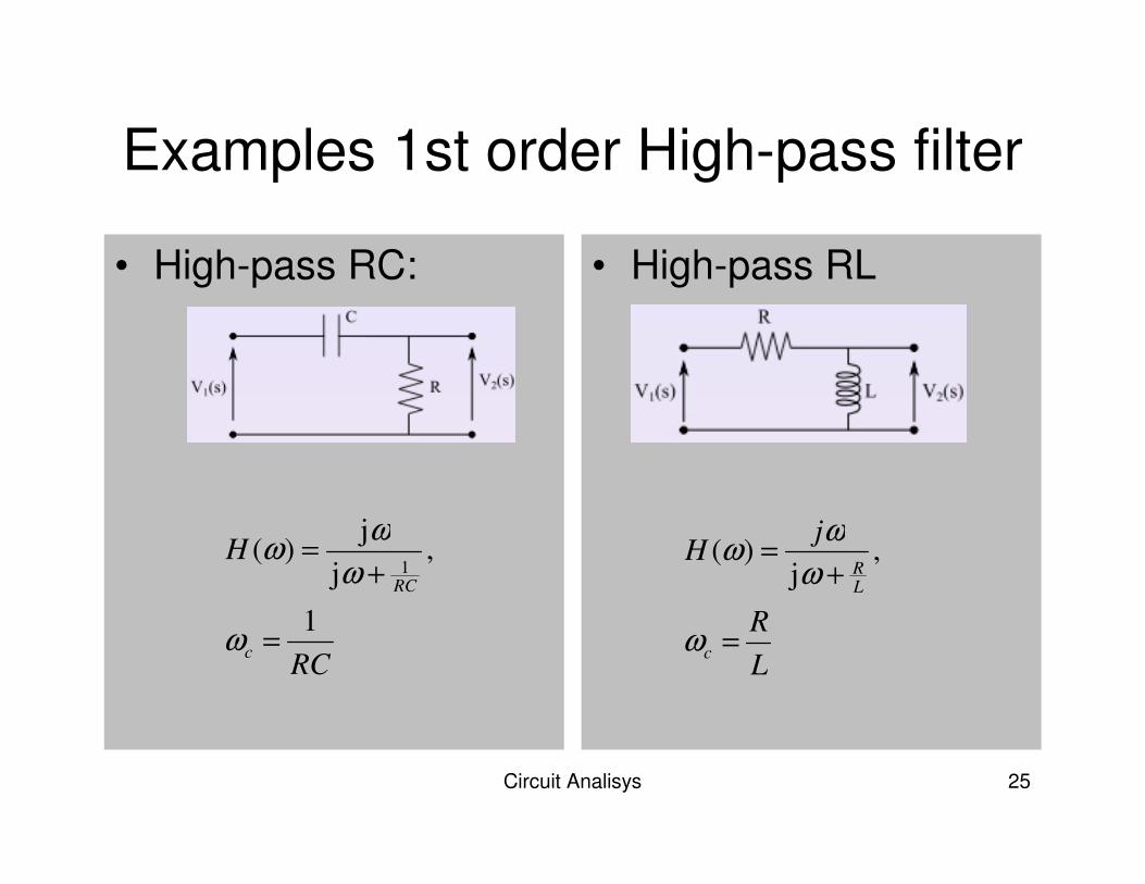
Circuit Analisys 25

Examples 1st order High-pass filter

• High-pass RC: • High-pass RL

L

R

jH

c

LR

=

+=

ω

ω

ωω ,

j)(

RC

H

c

RC

1

,j

j)(

1

=

+=

ω

ω

ωω

Circuit Analisys 26

2st order passive filters

• Transfer function:

• N2(s): Polynomial of order ≤ 2

• ξ: Damping coefficient

• ω0: Characteristic frequency of the filter

• Q=1/(2ξ): Quality factor of the circuit

• B= ω0 /Q: Band width of the circuit

2

0

2

2

2

00

2

2

21

2

2

0

)(

2

)()()(

ωωξω ω ++=

++=

++=

ss

sNk

ss

sNk

asas

sNksH

Q

Circuit Analisys 27

2nd order passive filters

• With 2nd order filter the four type of filters can be obtained (with 1st order only two)

• The poles of H(s) are:

• Depending on the value of ξ (or Q) we distinguish the following two poles:– Real and different (ξ>1 or Q<1/2)– Real and equal (ξ=1 or Q=1/2)– Complex conjugated (ξ<1 or Q>1/2)

• Depending on N2(s) we have the following special cases:

( ) ( )14j12

1j 202

02,1 −±−=−±−= QQ

sp

ωξξω

Circuit Analisys 28

2nd order filters

• Low-pass filter

• High-pass filter

• Band-pass filter

• Band-stop filter

Circuit Analisys 29

2nd order Low-pass filter

Example:

Circuit Analisys 30

2nd order High-pass filter

Example:

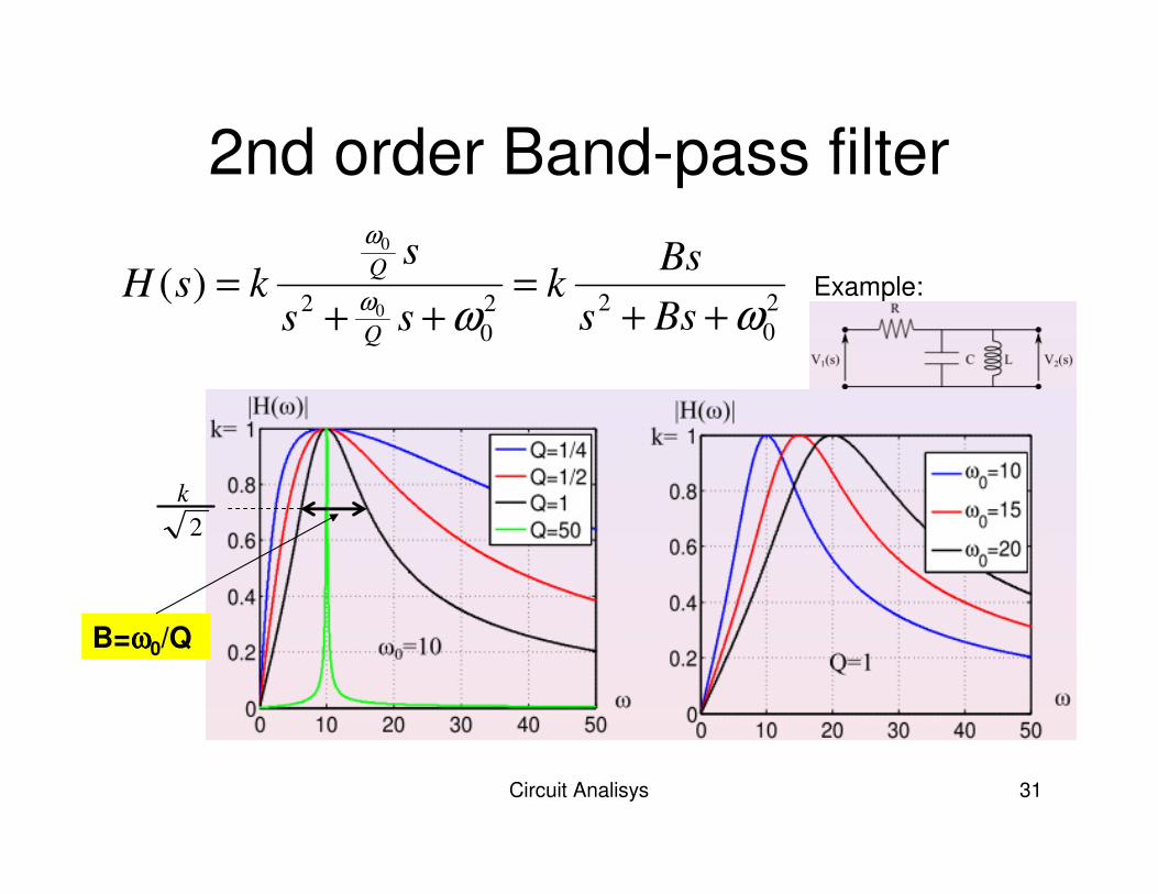
Circuit Analisys 31

2nd order Band-pass filter

B=ωωωω0/Q

2

k

2

0

22

0

2 0

0

)(ωωω

ω

++=

++=

Bss

Bsk

ss

sksH

Q

QExample:

Circuit Analisys 32

2nd order Band-stop filter

Example:

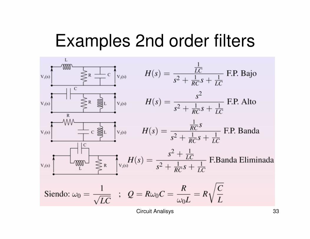
Circuit Analisys 33

Examples 2nd order filters