u. saravanan march 2013 · four concepts in mechanics and in section 1.2 we look at the equations...
TRANSCRIPT
Advanced Solid Mechanics
U. Saravanan
March 2013

ii

Contents
1 Introduction 11.1 Basic Concepts in Mechanics . . . . . . . . . . . . . . . . . . . 2
1.1.1 What is force? . . . . . . . . . . . . . . . . . . . . . . . 21.1.2 What is stress? . . . . . . . . . . . . . . . . . . . . . . 41.1.3 What is displacement? . . . . . . . . . . . . . . . . . . 61.1.4 What is strain? . . . . . . . . . . . . . . . . . . . . . . 7
1.2 Basic Equations in Mechanics . . . . . . . . . . . . . . . . . . 81.2.1 Equilibrium equations . . . . . . . . . . . . . . . . . . 81.2.2 Strain-Displacement relation . . . . . . . . . . . . . . . 91.2.3 Compatibility equation . . . . . . . . . . . . . . . . . . 111.2.4 Constitutive relation . . . . . . . . . . . . . . . . . . . 11
1.3 Classification of the Response of Materials . . . . . . . . . . . 131.3.1 Non-dissipative response . . . . . . . . . . . . . . . . . 131.3.2 Dissipative response . . . . . . . . . . . . . . . . . . . 15
1.4 Solution to Boundary Value Problems . . . . . . . . . . . . . . 191.4.1 Displacement method . . . . . . . . . . . . . . . . . . . 201.4.2 Stress method . . . . . . . . . . . . . . . . . . . . . . . 201.4.3 Semi-inverse method . . . . . . . . . . . . . . . . . . . 21
1.5 Summary . . . . . . . . . . . . . . . . . . . . . . . . . . . . . 22
2 Mathematical Preliminaries 232.1 Overview . . . . . . . . . . . . . . . . . . . . . . . . . . . . . . 232.2 Algebra of vectors . . . . . . . . . . . . . . . . . . . . . . . . . 232.3 Algebra of second order tensors . . . . . . . . . . . . . . . . . 28
2.3.1 Orthogonal tensor . . . . . . . . . . . . . . . . . . . . . 342.3.2 Symmetric and skew tensors . . . . . . . . . . . . . . . 352.3.3 Projection tensor . . . . . . . . . . . . . . . . . . . . . 372.3.4 Spherical and deviatoric tensors . . . . . . . . . . . . . 37
iii

iv CONTENTS
2.3.5 Polar Decomposition theorem . . . . . . . . . . . . . . 382.4 Algebra of fourth order tensors . . . . . . . . . . . . . . . . . 38
2.4.1 Alternate representation for tensors . . . . . . . . . . . 402.5 Eigenvalues, eigenvectors of tensors . . . . . . . . . . . . . . . 41
2.5.1 Square root theorem . . . . . . . . . . . . . . . . . . . 432.6 Transformation laws . . . . . . . . . . . . . . . . . . . . . . . 44
2.6.1 Vectorial transformation law . . . . . . . . . . . . . . . 442.6.2 Tensorial transformation law . . . . . . . . . . . . . . . 452.6.3 Isotropic tensors . . . . . . . . . . . . . . . . . . . . . 46
2.7 Scalar, vector, tensor functions . . . . . . . . . . . . . . . . . . 472.8 Gradients and related operators . . . . . . . . . . . . . . . . . 522.9 Integral theorems . . . . . . . . . . . . . . . . . . . . . . . . . 59
2.9.1 Divergence theorem . . . . . . . . . . . . . . . . . . . . 592.9.2 Stokes theorem . . . . . . . . . . . . . . . . . . . . . . 592.9.3 Green’s theorem . . . . . . . . . . . . . . . . . . . . . . 60
2.10 Summary . . . . . . . . . . . . . . . . . . . . . . . . . . . . . 632.11 Self-Evaluation . . . . . . . . . . . . . . . . . . . . . . . . . . 63
3 Kinematics 693.1 Overview . . . . . . . . . . . . . . . . . . . . . . . . . . . . . . 693.2 Body . . . . . . . . . . . . . . . . . . . . . . . . . . . . . . . . 693.3 Deformation Gradient . . . . . . . . . . . . . . . . . . . . . . 753.4 Lagrangian and Eulerian description . . . . . . . . . . . . . . 773.5 Displacement, velocity and acceleration . . . . . . . . . . . . . 79
3.5.1 Gradient of displacement . . . . . . . . . . . . . . . . . 803.5.2 Example . . . . . . . . . . . . . . . . . . . . . . . . . . 81
3.6 Transformation of curves, surfaces and volume . . . . . . . . . 823.6.1 Transformation of curves . . . . . . . . . . . . . . . . . 873.6.2 Transformation of areas . . . . . . . . . . . . . . . . . 933.6.3 Transformation of volumes . . . . . . . . . . . . . . . . 94
3.7 Properties of the deformation tensors . . . . . . . . . . . . . . 943.8 Strain Tensors . . . . . . . . . . . . . . . . . . . . . . . . . . . 953.9 Normal and shear strain . . . . . . . . . . . . . . . . . . . . . 98
3.9.1 Normal strain . . . . . . . . . . . . . . . . . . . . . . . 993.9.2 Principal strain . . . . . . . . . . . . . . . . . . . . . . 1003.9.3 Shear strain . . . . . . . . . . . . . . . . . . . . . . . . 1013.9.4 Transformation of linearized strain tensor . . . . . . . . 102
3.10 Homogeneous Motions . . . . . . . . . . . . . . . . . . . . . . 103
CONTENTS v
3.10.1 Rigid body Motion . . . . . . . . . . . . . . . . . . . . 1053.10.2 Uniaxial or equi-biaxial motion . . . . . . . . . . . . . 1063.10.3 Isochoric motions . . . . . . . . . . . . . . . . . . . . . 108
3.11 Compatibility condition . . . . . . . . . . . . . . . . . . . . . 1103.12 Summary . . . . . . . . . . . . . . . . . . . . . . . . . . . . . 1133.13 Self-Evaluation . . . . . . . . . . . . . . . . . . . . . . . . . . 114
4 Traction and Stress 1214.1 Overview . . . . . . . . . . . . . . . . . . . . . . . . . . . . . . 1214.2 Traction vectors and stress tensors . . . . . . . . . . . . . . . 122
4.2.1 Cauchy stress theorem . . . . . . . . . . . . . . . . . . 1244.2.2 Components of Cauchy stress . . . . . . . . . . . . . . 124
4.3 Normal and shear stresses . . . . . . . . . . . . . . . . . . . . 1274.4 Principal stresses and directions . . . . . . . . . . . . . . . . . 128
4.4.1 Maximum and minimum normal traction . . . . . . . . 1284.4.2 Maximum and minimum shear traction . . . . . . . . . 129
4.5 Stresses on a Octahedral plane . . . . . . . . . . . . . . . . . . 1314.6 Examples of state of stress . . . . . . . . . . . . . . . . . . . . 1324.7 Other stress measures . . . . . . . . . . . . . . . . . . . . . . . 135
4.7.1 Piola-Kirchhoff stress tensors . . . . . . . . . . . . . . 1354.7.2 Kirchhoff, Biot and Mandel stress measures . . . . . . 137
4.8 Summary . . . . . . . . . . . . . . . . . . . . . . . . . . . . . 1374.9 Self-Evaluation . . . . . . . . . . . . . . . . . . . . . . . . . . 138
5 Balance Laws 1435.1 Overview . . . . . . . . . . . . . . . . . . . . . . . . . . . . . . 1435.2 System . . . . . . . . . . . . . . . . . . . . . . . . . . . . . . . 1435.3 Conservation of Mass . . . . . . . . . . . . . . . . . . . . . . . 1445.4 Conservation of momentum . . . . . . . . . . . . . . . . . . . 148
5.4.1 Conservation of linear momentum . . . . . . . . . . . . 1525.4.2 Conservation of angular momentum . . . . . . . . . . . 154
5.5 Summary . . . . . . . . . . . . . . . . . . . . . . . . . . . . . 1585.6 Self-Evaluation . . . . . . . . . . . . . . . . . . . . . . . . . . 158
6 Constitutive Relations 1616.1 Overview . . . . . . . . . . . . . . . . . . . . . . . . . . . . . . 1616.2 Definition of elastic process . . . . . . . . . . . . . . . . . . . 1626.3 Restrictions on constitutive relation . . . . . . . . . . . . . . . 166
vi CONTENTS
6.3.1 Restrictions due to objectivity . . . . . . . . . . . . . . 1666.3.2 Restrictions due to Material Symmetry . . . . . . . . . 179
6.4 Isotropic Hooke’s law . . . . . . . . . . . . . . . . . . . . . . . 1826.5 Material parameters . . . . . . . . . . . . . . . . . . . . . . . 185
6.5.1 Young’s modulus and Poisson’s ratio . . . . . . . . . . 1856.5.2 Shear Modulus . . . . . . . . . . . . . . . . . . . . . . 1876.5.3 Bulk Modulus . . . . . . . . . . . . . . . . . . . . . . . 187
6.6 Restriction on material parameters . . . . . . . . . . . . . . . 1886.7 Internally constraint materials . . . . . . . . . . . . . . . . . . 189
6.7.1 Incompressible materials . . . . . . . . . . . . . . . . . 1926.8 Orthotropic Hooke’s law . . . . . . . . . . . . . . . . . . . . . 1956.9 Summary . . . . . . . . . . . . . . . . . . . . . . . . . . . . . 1986.10 Self-Evaluation . . . . . . . . . . . . . . . . . . . . . . . . . . 199
7 Boundary Value Problem: Formulation 2057.1 Overview . . . . . . . . . . . . . . . . . . . . . . . . . . . . . . 2057.2 Formulation of boundary value problem . . . . . . . . . . . . . 2077.3 Techniques to solve boundary value problems . . . . . . . . . . 209
7.3.1 Displacement method . . . . . . . . . . . . . . . . . . . 2097.3.2 Stress method . . . . . . . . . . . . . . . . . . . . . . . 211
7.4 Illustrative example . . . . . . . . . . . . . . . . . . . . . . . . 2177.4.1 Inflation of an annular cylinder . . . . . . . . . . . . . 2177.4.2 Uniaxial tensile loading of a plate with a hole . . . . . 224
7.5 General results . . . . . . . . . . . . . . . . . . . . . . . . . . 2327.5.1 Uniqueness of solution . . . . . . . . . . . . . . . . . . 2337.5.2 Principle of superposition . . . . . . . . . . . . . . . . 235
7.6 Summary . . . . . . . . . . . . . . . . . . . . . . . . . . . . . 2367.7 Self-Evaluation . . . . . . . . . . . . . . . . . . . . . . . . . . 237
8 Bending of Prismatic Straight Beams 2438.1 Overview . . . . . . . . . . . . . . . . . . . . . . . . . . . . . . 2438.2 Symmetrical bending . . . . . . . . . . . . . . . . . . . . . . . 248
8.2.1 Strength of materials solution . . . . . . . . . . . . . . 2488.2.2 2D Elasticity solution . . . . . . . . . . . . . . . . . . . 252
8.3 Asymmetrical bending . . . . . . . . . . . . . . . . . . . . . . 2748.4 Shear center . . . . . . . . . . . . . . . . . . . . . . . . . . . . 282
8.4.1 Illustrative examples . . . . . . . . . . . . . . . . . . . 2838.5 Summary . . . . . . . . . . . . . . . . . . . . . . . . . . . . . 292

CONTENTS vii
8.6 Self-Evaluation . . . . . . . . . . . . . . . . . . . . . . . . . . 293
9 End Torsion of Prismatic Bars 2979.1 Overview . . . . . . . . . . . . . . . . . . . . . . . . . . . . . . 2979.2 Twisting of thick walled closed section . . . . . . . . . . . . . 300
9.2.1 Circular bar . . . . . . . . . . . . . . . . . . . . . . . . 3039.3 Twisting of solid open section . . . . . . . . . . . . . . . . . . 304
9.3.1 Solid elliptical section . . . . . . . . . . . . . . . . . . 3139.3.2 Solid rectangular section . . . . . . . . . . . . . . . . . 3189.3.3 Thin rolled section . . . . . . . . . . . . . . . . . . . . 3239.3.4 Triangular cross section . . . . . . . . . . . . . . . . . 327
9.4 Twisting of hollow section . . . . . . . . . . . . . . . . . . . . 3299.4.1 Hollow elliptical section . . . . . . . . . . . . . . . . . 3339.4.2 Thin walled tubes . . . . . . . . . . . . . . . . . . . . . 334
9.5 Summary . . . . . . . . . . . . . . . . . . . . . . . . . . . . . 3379.6 Self-Evaluation . . . . . . . . . . . . . . . . . . . . . . . . . . 337
10 Bending of Curved Beams 34510.1 Overview . . . . . . . . . . . . . . . . . . . . . . . . . . . . . . 34510.2 Winkler-Bach formula for curved beams . . . . . . . . . . . . 34610.3 2D Elasticity solution for curved beams . . . . . . . . . . . . . 351
10.3.1 Pure bending . . . . . . . . . . . . . . . . . . . . . . . 35110.3.2 Curved cantilever beam under end load . . . . . . . . . 356
10.4 Summary . . . . . . . . . . . . . . . . . . . . . . . . . . . . . 35910.5 Self-Evaluation . . . . . . . . . . . . . . . . . . . . . . . . . . 360
11 Beam on Elastic Foundation 36311.1 Overview . . . . . . . . . . . . . . . . . . . . . . . . . . . . . . 36311.2 General formulation . . . . . . . . . . . . . . . . . . . . . . . . 36311.3 Example 1: Point load . . . . . . . . . . . . . . . . . . . . . . 36511.4 Example 2: Concentrated moment . . . . . . . . . . . . . . . . 37011.5 Example 3: Uniformly distributed load . . . . . . . . . . . . . 37211.6 Summary . . . . . . . . . . . . . . . . . . . . . . . . . . . . . 37311.7 Self-Evaluation . . . . . . . . . . . . . . . . . . . . . . . . . . 374

Chapter 1
Introduction
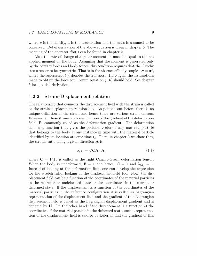
This course builds upon the concepts learned in the course “Mechanics ofMaterials” also known as “Strength of Materials”. In the “Mechanics of Ma-terials” course one would have learnt two new concepts “stress” and “strain”in addition to revisiting the concept of a “force” and “displacement” thatone would have mastered in a first course in mechanics, namely “EngineeringMechanics”. Also one might have been exposed to four equations connect-ing these four concepts, namely strain-displacement equation, constitutiveequation, equilibrium equation and compatibility equation. Figure 1.1 pic-torially depicts the concepts that these equations relate. Thus, the straindisplacement relation allows one to compute the strain given a displacement;constitutive relation gives the value of stress for a known value of the strainor vice versa; equilibrium equation, crudely, relates the stresses developed inthe body to the forces and moment applied on it; and finally compatibilityequation places restrictions on how the strains can vary over the body sothat a continuous displacement field could be found for the assumed strainfield.
In this course too we shall be studying the same four concepts and fourequations. While in the “mechanics of materials” course, one was introducedto the various components of the stress and strain, namely the normal andshear, in the problems that was solved not more than one component of thestress or strain occurred simultaneously. Here we shall be studying theseproblems in which more than one component of the stress or strain occurssimultaneously. Thus, in this course we shall be generalizing these conceptsand equations to facilitate three dimensional analysis of structures.
Before venturing into the generalization of these concepts and equations,
1

2 CHAPTER 1. INTRODUCTION
Force Displacement
Stress StrainConstitutiverelation
Strain-displacementrelation
Equilibrium e uations
Compatibilityequationsq
Figure 1.1: Basic concepts and equations in mechanics
a few drawbacks of the definitions and ideas that one might have acquiredfrom the previous course needs to be highlighted and clarified. This weshall do in sections 1.1 and 1.2. Specifically, in section 1.1 we look at thefour concepts in mechanics and in section 1.2 we look at the equations inmechanics. These sections also serve as a motivation for the mathematicaltools that we would be developing in chapter 2. Then, in section 1.3 we lookinto various idealizations of the response of materials and the mathematicalframework used to study them. However, in this course we shall be onlyfocusing on the elastic response or more precisely, non-dissipative responseof the materials. Finally, in section 1.4 we outline three ways by which wecan solve problems in mechanics.
1.1 Basic Concepts in Mechanics
1.1.1 What is force?
Force is a mathematical idea to study the motion of bodies. It is not “real”as many think it to be. However, it can be associated with the twitching ofthe muscle, feeling of the burden of mass, linear translation of the motor, soon and so forth. Despite seeing only displacements we relate it to its causethe force, as the concept of force has now been ingrained.

1.1. BASIC CONCEPTS IN MECHANICS 3
Let us see why force is an idea that arises from mathematical need. Say,the position1 (xo) and velocity (vo) of the body is known at some time, t= to, then one is interested in knowing where this body would be at a latertime, t = t1. It turns out that mathematically, if the acceleration (a) of thebody at any later instant in time is specified then the position of the bodycan be determined through Taylor’s series. That is if
a =d2x
dt2= fa(t), (1.1)
then from Taylor’s series
x1 = x(t1) = x(to) +dx
dt
∣∣∣∣t=to
(t1 − to) +d2x
dt2
∣∣∣∣t=to
(t1 − to)2
2!
+d3x
dt3
∣∣∣∣t=to
(t1 − to)3
3!+d4x
dt4
∣∣∣∣t=to
(t1 − to)4
4!+ . . . , (1.2)
which when written in terms of xo, vo and a reduces to2
x1 = xo + vo(t1 − to) + fa(to)(t1 − to)2
2!+dfadt
∣∣∣∣t=to
(t1 − to)3
3!
+d2fadt2
∣∣∣∣t=to
(t1 − to)4
4!+ . . . . (1.3)
Thus, if the function fa is known then the position of the body at any otherinstant in time can be determined. This function is nothing but force perunit mass3, as per Newton’s second law which gives a definition for the force.This shows that force is a function that one defines mathematically so thatthe position of the body at any later instance can be obtained from knowingits current position and velocity.
It is pertinent to point out that this function fa could also be prescribedusing the position, x and velocity, v of the body which are themselves func-tion of time, t and hence fa would still be a function of time. Thus, fa =g(x(t),v(t), t). However, fa could not arbitrarily depend on t, x and v. At
1Any bold small case alphabet denotes a vector. Example a, x.2Here it is pertinent to note that the subscripts denote the instant in time when position
or velocity is determined. Thus, xo denotes the position at time to and x1 denotes theposition at time t1.
3Here the mass of the body is assumed to be a constant.

4 CHAPTER 1. INTRODUCTION
this point it suffices to say that the other two laws of Newton and certainobjectivity requirements have to be met by this function. We shall see whatthese objectivity requirements are and how to prescribe functions that meetthis requirement subsequently in chapter - 6.
Next, let us understand what kind of quantity is force. In other words isforce a scalar or vector and why? Since, position is a vector and accelerationis second time derivative of position, it is also a vector. Then, it follows fromequation (1.1) that fa also has to be a vector. Therefore, force is a vectorquantity. Numerous experiments also show that addition of forces followvector addition law (or the parallelogram law of addition). In chapter 2 weshall see how the vector addition differs from scalar addition. In fact it is thisaddition rule that distinguishes a vector from a scalar and hence confirmsthat force is a vector.
As a summary, we showed that force is a mathematical construct whichis used to mathematically describe the motion of bodies.
1.1.2 What is stress?
As is evident from figure 1.1, stress is a quantity derived from force. Thecommonly stated definitions in an introductory course in mechanics for stressare:
1. Stress is the force acting per unit area
2. Stress is the resistance offered by the body to a force acting on it
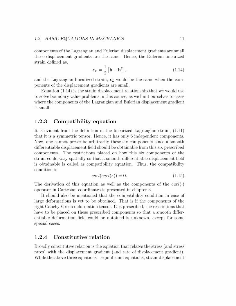
While the first definition tells how to compute the stress from the force, thisdefinition holds only for simple loading case. One can construct a numberof examples where definition 1 does not hold. The following two cases arepresented just as an example. Case -1: A cantilever beam of rectangular crosssection with a uniform pressure, p, applied on the top surface, as shown infigure 1.2a. According to the definition 1 the stress in the beam should bep, but it is not. Case -2: An annular cylinder subjected to a pressure, pat its inner surface, as shown in figure 1.2b. The net force acting on thecylinder is zero but the stresses are not zero at any location. Also, the stressis not p, anywhere in the interior of the cylinder. This being the state ofthe first definition, the second definition is of little use as it does not tellhow to compute the stress. These definitions does not tell that there arevarious components of the stress nor whether the area over which the force

1.1. BASIC CONCEPTS IN MECHANICS 5
P
(a) A cantilever beam with uniformpressure applied on its top surface.
P
(b) An annular cylinder subjected tointernal pressure.
Figure 1.2: Structures subjected to pressure loading
is considered to be distributed is the deformed or the undeformed. They donot distinguish between traction (or stress vector), t(n) and stress tensor, σ.
Traction is the distributed force acting per unit area of a cut surfaceor boundary of the body. This traction apart from varying spatially andtemporally also depends on the plane of cut characterized by its normal.This quantity integrated over the cut surface gives the net force acting onthat surface. Consequently, since force is a vector quantity this traction isalso a vector quantity. The component of the traction along the normaldirection4, n is called as the normal stress (σ(n)). The magnitude of thecomponent of the traction5 acting parallel to the plane is called as the shearstress (τ(n)).
If the force is distributed over the deformed area then the correspondingtraction is called as the Cauchy traction (t(n)) and if the force is distributedover the undeformed or original area that traction is called as the Piolatraction (p(n)). If the deformed area does not change significantly from the
4 Here n is a unit vector.5Recognize that there would be two components of traction acting on the plane of cut.
Shear stress is neither of those components. For example, if traction on a plane whosenormal is ez is, t(ez) = axex + ayey + azez, then the normal stress σ(ez) = az and the
shear stress τ(ez) =√a2x + a2y. See chapter 4 for more details.
6 CHAPTER 1. INTRODUCTION
original area, then both these traction would have nearly the same magnitudeand direction. More details about these traction is presented in chapter 4.
The stress tensor, is a linear function (crudely, a matrix) that relates thenormal vector, n to the traction acting on that plane whose normal is n. Thestress tensor could vary spatially and temporally but does not change withthe plane of cut. Just like there is Cauchy and Piola traction, depending onover which area the force is distributed, there are two stress tensors. TheCauchy (or true) stress tensor, σ and the Piola-Kirchhoff stress tensor (P).While these two tensors may nearly be the same when the deformed area isnot significantly different from the original area, qualitatively these tensorsare different. To satisfy the moment equilibrium in the absence of bodycouples, Cauchy stress tensor has to be symmetric tensor (crudely, symmetricmatrix) and Piola-Kirchhoff stress tensor cannot be symmetric. In fact thetranspose of the Piola-Kirchhoff stress tensor is called as the engineeringstress or nominal stress. Moreover, there are many other stress measuresobtained from the Cauchy stress and the gradient of the displacement whichshall be studied in chapter 4.
1.1.3 What is displacement?
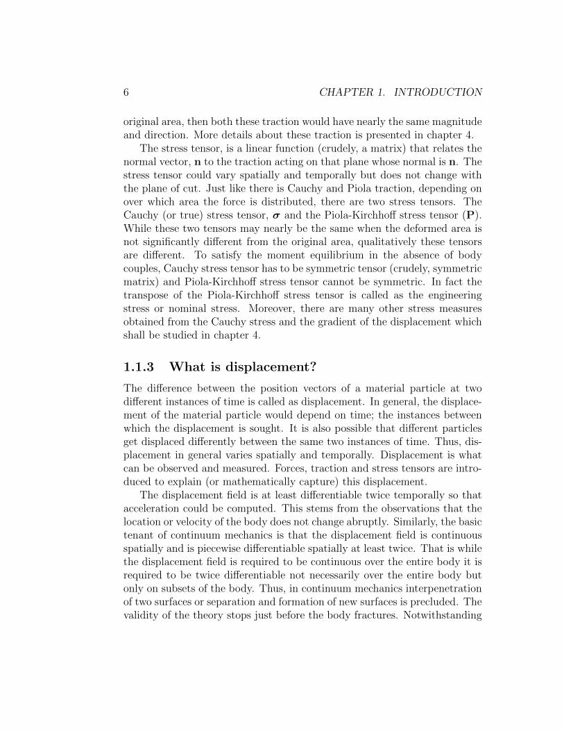
The difference between the position vectors of a material particle at twodifferent instances of time is called as displacement. In general, the displace-ment of the material particle would depend on time; the instances betweenwhich the displacement is sought. It is also possible that different particlesget displaced differently between the same two instances of time. Thus, dis-placement in general varies spatially and temporally. Displacement is whatcan be observed and measured. Forces, traction and stress tensors are intro-duced to explain (or mathematically capture) this displacement.
The displacement field is at least differentiable twice temporally so thatacceleration could be computed. This stems from the observations that thelocation or velocity of the body does not change abruptly. Similarly, the basictenant of continuum mechanics is that the displacement field is continuousspatially and is piecewise differentiable spatially at least twice. That is whilethe displacement field is required to be continuous over the entire body it isrequired to be twice differentiable not necessarily over the entire body butonly on subsets of the body. Thus, in continuum mechanics interpenetrationof two surfaces or separation and formation of new surfaces is precluded. Thevalidity of the theory stops just before the body fractures. Notwithstanding

1.1. BASIC CONCEPTS IN MECHANICS 7
this many attempt to use continuum mechanics concepts to understand theprocess of fracture.
A body is said to undergo rigid body displacement if the distance betweenany two particles that belongs to the body remains unchanged. That is ina rigid body displacement the particles that belong to a body do not moverelative to each other. A body is said to be rigid if it always undergoes onlyrigid body displacement under action of any force. On the other hand, a bodyis said to be deformable if it allows relative displacement of its particles underthe action of some force. Though, all real bodies are deformable, at timesone could idealize a given body as rigid under the action of certain forces.
1.1.4 What is strain?
One observes that rigid body displacements of the body does not give raiseto any stresses. Further, stresses are induced only when there is relativedisplacement of the material particles. Consequently, one requires a measure(or metric) for this relative displacement so that it can be related to thestress. The unique measure of relative displacement is the stretch ratio,λ(A), defined as the ratio of the deformed length to the original length of amaterial fiber along a given direction, A. (Note that here A is a unit vector.)However, this measure has the drawback that when the body is not deformedthe stretch ratio is 1 (by virtue of the deformed length being same as theoriginal length) and hence inconvenient to write the constitutive relation ofthe form
σ(A) = f(λ(A)), (1.4)
where σ(A) denotes the normal stress on a plane whose normal is A. Sincethe stress is zero when the body is not deformed, the function f should besuch that f(1) = 0. Mathematical implementation of this condition thatf(1) = 0 and that f be a one to one function is thought to be difficult whenf is a nonlinear function of λ(A). Consequently, another measure of relativedisplacement is sought which would be 0 when the body is not deformed andless than zero when compressed and greater than zero when stretched. Thismeasure is called as the strain, ε(A). There is no unique way of obtaining thestrain from the stretch ratio. The following functions satisfy the requirementof the strain:
ε(A) =λm(A) − 1
m, ε(A) = ln(λ(A)), (1.5)

8 CHAPTER 1. INTRODUCTION
where m is some real number and ln stands for natural logarithm. Thus, ifm = 1 in (1.5a) then the resulting strain is called as the engineering strain,if m = −1, it is called as the true strain, if m = 2 it is Cauchy-Green strain.The second function wherein ε(A) = ln(λ(A)), is called as the Hencky strainor the logarithmic strain.
Just like the traction and hence the normal stress changes with the ori-entation of the plane, the stretch ratio also changes with the orientationalong which it is measured. We shall see in chapter 3 that a tensor calledthe Cauchy-Green deformation tensor carries all the information required tocompute the stretch ratio along any direction. This is akin to the stress ten-sor which when known we could compute the traction or the normal stressin any plane.
1.2 Basic Equations in Mechanics
Having gained a superficial understanding of the four concepts in mechanicsnamely the force, stress, displacement and strain, let us look at the fourequations that connect these concepts and the reasoning used to obtain them.
1.2.1 Equilibrium equations
Equilibrium equations are Newton’s second law which states that the rate ofchange of linear momentum would be equal in magnitude and direction tothe net applied force. Deformable bodies are subjected to two kinds of forces,namely, contact force and body force. As the name suggest the contact forcearises by virtue of the body being in contact with its surroundings. Tractionarises only due to these contact force and hence so does the stress tensor.The magnitude of the contact force depends on the contact area betweenthe body and its surroundings. On the other hand, the body forces areaction at a distance forces. Examples of body force are gravitational force,electromagnetic force. The magnitude of these body forces depend on themass of the body and hence are generally expressed as per unit mass of thebody and denoted by b.
On further assuming that the Newton’s second law holds for any subpartof the body and that the stress field is continuously differentiable within thebody the equilibrium equations can be written as:
div(σ) + ρb = ρa, (1.6)
1.2. BASIC EQUATIONS IN MECHANICS 9
where ρ is the density, a is the acceleration and the mass is assumed to beconserved. Detail derivation of the above equation is given in chapter 5. Themeaning of the operator div(·) can be found in chapter 2.
Also, the rate of change of angular momentum must be equal to the netapplied moment on the body. Assuming that the moment is generated onlyby the contact forces and body forces, this condition requires that the Cauchystress tensor to be symmetric. That is in the absence of body couples, σ = σt,where the superscript (·)t denotes the transpose. Here again the assumptionsmade to obtain the force equilibrium equation (1.6) should hold. See chapter5 for detailed derivation.
1.2.2 Strain-Displacement relation
The relationship that connects the displacement field with the strain is calledas the strain displacement relationship. As pointed out before there is nounique definition of the strain and hence there are various strain tensors.However, all these strains are some function of the gradient of the deformationfield, F; commonly called as the deformation gradient. The deformationfield is a function that gives the position vector of any material particlethat belongs to the body at any instance in time with the material particleidentified by its location at some time to. Then, in chapter 3 we show that,the stretch ratio along a given direction A is,
λ(A) =√
CA ·A, (1.7)
where C = FtF, is called as the right Cauchy-Green deformation tensor.When the body is undeformed, F = 1 and hence, C = 1 and λ(A) = 1.Instead of looking at the deformation field, one can develop the expressionfor the stretch ratio, looking at the displacement field too. Now, the dis-placement field can be a function of the coordinates of the material particlesin the reference or undeformed state or the coordinates in the current ordeformed state. If the displacement is a function of the coordinates of thematerial particles in the reference configuration it is called as Lagrangianrepresentation of the displacement field and the gradient of this Lagrangiandisplacement field is called as the Lagrangian displacement gradient and isdenoted by H. On the other hand if the displacement is a function of thecoordinates of the material particle in the deformed state, such a representa-tion of the displacement field is said to be Eulerian and the gradient of this

10 CHAPTER 1. INTRODUCTION
Eulerian displacement field is called as the Eulerian displacement gradientand is denoted by h. Then it can be shown that (see chapter 3),
F = H + 1, F−1 = 1− h, (1.8)
where, 1 stands for identity tensor (see chapter 2 for its definition). Now,the right Cauchy-Green deformation tensor can be written in terms of theLagrangian displacement gradient as,
C = 1 + H + Ht + HtH. (1.9)
Note that the if the body is undeformed then H = 0. Hence, if one cannotsee the displacement of the body then it is likely that the components ofthe Lagrangian displacement gradient are going to be small, say of order10−3. Then, the components of the tensor HtH are going to be of the order10−6. Hence, the equation (1.9) for this case when the components of theLagrangian displacement gradient is small can be approximately calculatedas,
C = 1 + 2εL, (1.10)
where
εL =1
2
[H + Ht
], (1.11)
is called as the linearized Lagrangian strain. We shall see in chapter 3 thatwhen the components of the Lagrangian displacement gradient is small, thestretch ratio (1.7) reduces to
λA = 1 + εLA ·A. (1.12)
Thus we find that εL contains information about changes in length alongany given direction, A when the components of the Lagrangian displacementgradient are small. Hence, it is called as the linearized Lagrangian strain.We shall in chapter 3 derive the various strain tensors corresponding to thevarious definition of strains given in equation (1.5).
Further, since FF−1 = 1, it follows from (1.8) that
H = h + Hh, (1.13)
which when the components of both the Lagrangian and Eulerian displace-ment gradient are small can be approximated as H = h. Thus, when the
1.2. BASIC EQUATIONS IN MECHANICS 11
components of the Lagrangian and Eulerian displacement gradients are smallthese displacement gradients are the same. Hence, the Eulerian linearizedstrain defined as,
εE =1
2
[h + ht
], (1.14)
and the Lagrangian linearized strain, εL would be the same when the com-ponents of the displacement gradients are small.
Equation (1.14) is the strain displacement relationship that we would useto solve boundary value problems in this course, as we limit ourselves to caseswhere the components of the Lagrangian and Eulerian displacement gradientis small.
1.2.3 Compatibility equation
It is evident from the definition of the linearized Lagrangian strain, (1.11)that it is a symmetric tensor. Hence, it has only 6 independent components.Now, one cannot prescribe arbitrarily these six components since a smoothdifferentiable displacement field should be obtainable from this six prescribedcomponents. The restrictions placed on how this six components of thestrain could vary spatially so that a smooth differentiable displacement fieldis obtainable is called as compatibility equation. Thus, the compatibilitycondition is
curl(curl(ε)) = 0. (1.15)
The derivation of this equation as well as the components of the curl(·)operator in Cartesian coordinates is presented in chapter 3.
It should also be mentioned that the compatibility condition in case oflarge deformations is yet to be obtained. That is if the components of theright Cauchy-Green deformation tensor, C is prescribed, the restrictions thathave to be placed on these prescribed components so that a smooth differ-entiable deformation field could be obtained is unknown, except for somespecial cases.
1.2.4 Constitutive relation
Broadly constitutive relation is the equation that relates the stress (and stressrates) with the displacement gradient (and rate of displacement gradient).While the above three equations - Equilibrium equations, strain-displacement

12 CHAPTER 1. INTRODUCTION
relation, compatibility equations - are independent of the material that thebody is made up of and/or the process that the body is subjected to, theconstitutive relation is dependent on the material and the process. Consti-tutive relation is required to bring in the dependance of the material in theresponse of the body and to have as many equations as there are unknowns,as will be shown in chapter 6.
The fidelity of the predictions, namely the likely displacement or stressfor a given force depends only on the constitutive relation. This is so becausethe other three equations are the same irrespective of the material that thebody is made up of. Consequently, a lot of research is being undertaken toarrive at better constitutive relations for materials.
It is difficult to have a constitutive relation that could describe the re-sponse of a material subjected to any process. Hence, usually constitutiverelations are prescribed for a particular process that the material undergoes.The variables in the constitutive relation depends on the process that is beingstudied. The same material could undergo different processes depending onthe stimuli; for example, the same material could respond elastically or plas-tically depending on say, the magnitude of the load or temperature. Henceit is only apt to qualify the process and not the material. However, it iscustomary to qualify the material instead of the process too. This we shalldesist.
Traditionally, the constitutive relation is said to depend on whether thegiven material behaves like a solid or fluid and one elaborates on how toclassify a given material as a solid or a fluid. A material that is not a solidis defined as a fluid. This means one has to define what a solid is. A coupleof definitions of a solid are listed below:
1. Solid is one which can resist sustained shear forces without continuouslydeforming
2. Solid is one which does not take the shape of the container
Though these definitions are intuitive they are ambiguous. A class of mate-rials called “viscoelastic solids”, neither take the shape of the container norresist shear forces without continuously deforming. Also, the same mate-rial would behave like a solid, like a mixture of a solid and a fluid or like afluid depending on say, the temperature and the mechanical stress it is beingsubjected to. These prompts us to say that a given material behaves in asolid-like or fluid-like manner. However, as we shall see, this classification of

1.3. CLASSIFICATION OF THE RESPONSE OF MATERIALS 13
a given material as solid or fluid is immaterial. If one appeals to thermody-namics for the classification of the processes, the response of materials couldbe classified based on (1) Whether there is conversion of energy from oneform to another during the process, and (2) Whether the process is thermo-dynamically equilibrated. Though, in the following section, we classify theresponse of materials based on thermodynamics, we also give the commonlystated definitions and discuss their shortcomings. In this course, as well asin all these classifications, it is assumed that there are no chemical changesoccurring in the body and hence the composition of the body remains aconstant.
1.3 Classification of the Response of Materi-
als
First, it should be clarified that one should not get confused with the realbody and its mathematical idealization. Modeling is all about idealizationsthat lead to predictions that are close to observations. To illustrate, theearth and the sun are assumed as point masses when one is interested inplanetary motion. The same earth is assumed as a rigid sphere if one isinterested in studying the eclipse. These assumptions are made to make theresulting problem tractable without losing on the required accuracy. In thesame sprit, the all material responses, some amount of mechanical energy isconverted into other forms of energy. However, in some cases, this loss in themechanical energy is small that it can be idealized as having no loss, i.e., anon-dissipative process.
1.3.1 Non-dissipative response
A response is said to be non-dissipative if there is no conversion of mechanicalenergy to other forms of energy, namely heat energy. Commonly, a materialresponding in this fashion is said to be elastic. The common definitions ofelastic response,
1. If the body’s original size and shape can be recovered on unloading,the loading process is said to be elastic.
2. Processes in which the state of stress depends only on the current strain,is said to be elastic.

14 CHAPTER 1. INTRODUCTION
The first definition is of little use, because it requires one to do a complimen-tary process (unloading) to decide on whether the process that needs to beclassified as being elastic. The second definition, though useful for decidingon the variables in the constitutive relation, it also requires one to do a com-plimentary process (unload and load again) to decide on whether the firstprocess is elastic. The definition based on thermodynamics does not sufferfrom this drawback. In chapter 6 we provide examples where these three def-initions are not equivalent. However, many processes (approximately) satisfyall the three definitions.
This class of processes also proceeds through thermodynamically equili-brated states. That is, if the body is isolated at any instant of loading (ordisplacement) then the stress, displacement, internal energy, entropy do notchange with time.
Ideal gas, a fluid is the best example of a material that responds in anon-dissipative manner. Metals up to a certain stress level, called the yieldstress, are also idealized as responding in a non dissipative manner. Thus,the notion that only solids respond in a non-dissipative manner is not correct.
Thus, for these non-dissipative, thermodynamically equilibrated processesthe Cauchy stress and the deformation gradient can in general be relatedthrough an implicit function. That is, for isotropic materials (see chapter6 for when a material is said to be isotropic), f(σ,F) = 0. However, inclassical elasticity it is customary to assume that Cauchy stress in a isotropicmaterial is a function of the deformation gradient, σ = f(F). On requiringthe restriction6 due to objectivity and second law of thermodynamics to hold,it can be shown that if σ = f(F), then
σ =∂ψR∂J3
1 +2
J3
[∂ψR∂J1
B− ∂ψR∂J2
B−1
], (1.16)
where ψR = ψR(J1, J2, J3) is the Helmoltz free energy defined per unit volumein the reference configuration, also called as the stored energy, B = FFt andJ1 = tr(B), J2 = tr(B−1), J3 =
√det(B). When the components of the
displacement gradient is small, then (1.16) reduces to,
σ = tr(ε)λ1 + 2µε, (1.17)
on neglecting the higher powers of the Lagrangian displacement gradientand where λ and µ are called as the Lame constants. The equation (1.17) is
6See chapter 6 for more details about these restrictions.
1.3. CLASSIFICATION OF THE RESPONSE OF MATERIALS 15
the famous Hooke’s law for isotropic materials. In this course Hooke’s lawis the constitutive equation that we shall be using to solve boundary valueproblems.
Before concluding this section, another misnomer needs to be clarified.As can be seen from equation (1.16) the relationship between Cauchy stressand the displacement gradient can be nonlinear when the response is non-dissipative. Only sometimes as in the case of the material obeying Hooke’slaw is this relationship linear. It is also true that if the response is dissi-pative, the relationship between the stress and the displacement gradient isalways nonlinear. However, nonlinear relationship between the stress and thedisplacement gradient does not mean that the response is dissipative. Thatis, nonlinear relationship between the stress and the displacement gradientis only a necessary condition for the response to be dissipative but not asufficient condition.
1.3.2 Dissipative response
A response is said to be dissipative if there is conversion of mechanical energyto other forms of energy. A material responding in this fashion is popularlysaid to be inelastic. There are three types of dissipative response, which weshall see in some detail.
Plastic response
A material is said to deform plastically if the deformation process proceedsthrough thermodynamically equilibrated states but is dissipative. That is,if the body is isolated at any instant of loading (or displacement) then thestress, displacement, internal energy, entropy do not change with time. Byvirtue of the process being dissipative, the stress at an instant would dependon the history of the deformation. However, the stress does not depend on therate of loading or displacement by virtue of the process proceeding throughthermodynamically equilibrated states.
For plastic response, the classical constitutive relation is assumed to beof the form,
σ = f(F,Fp, q1, q2), (1.18)
where Fp, q1, q2 are internal variables whose values could change with de-formation and/or stress. For illustration, we have used two scalar internalvariables and one second order tensor internal variable while there can be any

16 CHAPTER 1. INTRODUCTION
number of tensor or scalar internal variables. In some theories the internalvariables are given a physical interpretation but in general, these variableneed not have any meaning and are proposed for mathematical modelingpurpose only.
Thus, when a material deforms plastically, it does not return back toits original shape when unloaded; there would be a permanent deformation.Hence, the process is irreversible. The response does not depend on the rateof loading (or displacement). Metals like steel at room temperature respondplastically when stressed above a particular limit, called the yield stress.
Viscoelastic response
If the dissipative process proceeds through states that are not in thermody-namic equilibrium7, then it is said to be viscoelastic. Therefore, if a body isisolated at some instant of loading (or displacement) then the displacement(or the stress) continues to change with time. A viscoelastic material whensubjected to constant stress would result in a deformation that changes withtime which is called as creep. Also, when a viscoelastic material is subjectedto a constant deformation field, its stress changes with time and this is calledas stress relaxation. This is in contrary to a elastic or plastic material whichwhen subjected to a constant stress would have a constant strain.
The constitutive relation for a viscoelastic response is of the form,
f(σ,F, σ, F) = 0, (1.19)
where σ denotes the time derivative of stress and F time derivative of thedeformation gradient. Though here we have truncated to first order timederivatives, the general theory allows for higher order time derivatives too.
Thus, the response of a viscoelastic material depends on the rate at whichit is loaded (or displaced) apart from the history of the loading (or dis-placement). The response of a viscoelastic material changes depending onwhether load is controlled or displacement is controlled. This process toois irreversible and there would be unrecovered deformation immediately onremoval of the load. The magnitude of unrecovered deformation after a longtime (asymptotically) would tend to zero or remain the same constant valuethat it is immediately after the removal of load.
7A body is said to be in thermodynamic equilibrium if no quantity that describes itsstate changes when it is isolated from its surroundings. A body is said to be isolated whenthere is no mass or energy flux in to or out of the body.

1.3. CLASSIFICATION OF THE RESPONSE OF MATERIALS 17
Constitutive relations of the form,
σ = f(F), (1.20)
which is a special case of the viscoelastic constitutive relation (1.19), is thatof a viscous fluid.
In some treatments of the subject, a viscoelastic material would be saidto be a combination of a viscous fluid and an elastic solid and the viscoelasticmodels are obtained by combining springs and dashpots. There are severalphilosophical problems associated with this viewpoint about which we cannotelaborate here.
Viscoplastic response
This process too is dissipative and proceeds through states that are notin thermodynamic equilibrium. However, in order to model this class ofresponse the constitutive relation has to be of the form,
f(σ,F, σ, F,Fp, q1, q2) = 0, (1.21)
where Fp, q1, q2 are the internal variables whose values could change withdeformation and/or stress. Their significance is same as that discussed forplastic response. As can be easily seen the constitutive relation form forthe viscoplastic response (1.21) encompasses viscoelastic, plastic and elasticresponse as a special case.
In this case, constant load causes a deformation that changes with time.Also, a constant deformation causes applied load to change with time. Theresponse of the material depends on the rate of loading or displacement.The process is irreversible and there would be unrecovered deformation onremoval of load. The magnitude of this unrecovered deformation varies withrate of loading, time and would tend to a value which is not zero. Thisdependance of the constant value that the unrecovered deformation tendson the rate of loading, could be taken as the characteristic of viscoplasticresponse.
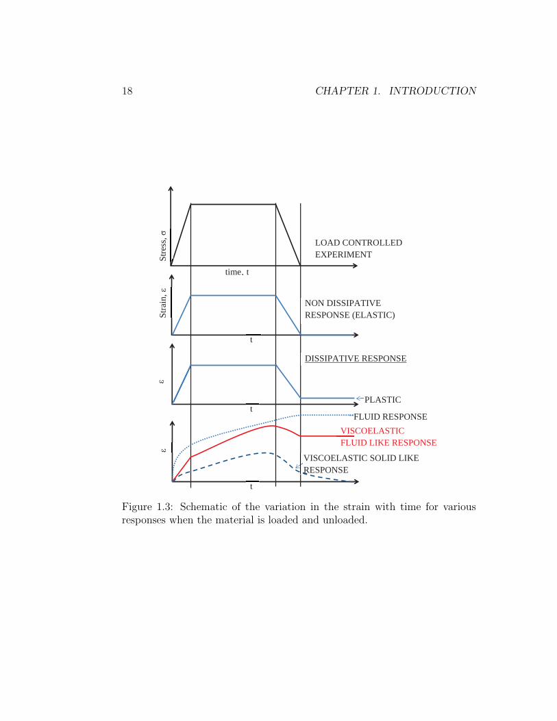
Figure 1.3 shows the typical variation in the strain for various responseswhen the material is loaded, held at a constant load and unloaded, as dis-cussed above. This kind of loading is called as the creep and recovery loading,helps one to distinguish various kinds of responses.
As mentioned already, in this course we shall focus on the elastic or non-dissipative response only.
18 CHAPTER 1. INTRODUCTION
FLUID RESPONSE
LOAD CONTROLLED EXPERIMENT
NON DISSIPATIVE RESPONSE (ELASTIC)
DISSIPATIVE RESPONSE
PLASTIC
VISCOELASTIC FLUID LIKE RESPONSE
VISCOELASTIC SOLID LIKE RESPONSE
t
t
t
Stre
ss, σ
ε
ε St
rain
, ε
time‚ t
Figure 1.3: Schematic of the variation in the strain with time for variousresponses when the material is loaded and unloaded.
1.4. SOLUTION TO BOUNDARY VALUE PROBLEMS 19
1.4 Solution to Boundary Value Problems
A boundary value problem is one in which we specify the traction applied onthe surface of a body and/or displacement of the boundary of a body andare interested in finding the displacement and/or the stress at any interiorpoint in the body or on part of the boundary where they were not specified.This specification of the boundary traction and/or displacement is calledas boundary condition. The boundary condition is in a sense constitutiverelation for the boundary. It tells how the body and its surroundings interact.Thus, in a boundary value problem one needs to prescribe the geometry of thebody, the constitutive relation for the material that the body is made up of forthe process it is going to be subjected to and the boundary condition. Usingthis information one needs to find the displacement and stress that the bodyis subjected to. The so found displacement and stress field should satisfy theequilibrium equations, constitutive relations, compatibility conditions andboundary conditions.
The purpose of formulating and solving a boundary value problem is to:
1. To ensure the stresses are within prescribed limits
2. To ensure that the displacements are within prescribed limits
3. To find the distribution of forces and moments on part of the boundarywhere displacements are specified
There are four type of boundary conditions. They are
1. Displacement boundary condition: Here the displacement of theentire boundary of the body alone is specified. This is also called asDirichlet boundary condition
2. Traction boundary condition: Here the traction on the entire bound-ary of the body alone is specified. This is also called as Neumannboundary condition
3. Mixed boundary condition: Here the displacement is specified onpart of the boundary and traction is specified on the remaining part ofthe boundary. Both traction as well as displacement are not specifiedover any part of boundary

20 CHAPTER 1. INTRODUCTION
4. Robin boundary condition: Here both the displacement and thetraction are specified on the same part of the boundary.
There are three methods by which the displacement and stress field inthe body can be found, satisfying all the required governing equations andthe boundary conditions. Outline of these methods are presented next. Thechoice of a method depends on the type of boundary condition.
1.4.1 Displacement method
Here displacement field is taken as the basic unknown. Then, using thestrain displacement relation, (1.14) the strain is computed. This strain insubstituted in the constitutive relation, (1.17) to obtain the stress. The stressis then substituted in the equilibrium equation (1.6) to obtain 3 second orderpartial differential equations in terms of the components of the displacementfield as,
(λ+ µ)grad(div(u)) + µ∆u + ρb = ρd2u
dt2, (1.22)
where ∆(·) stands for the Laplace operator and t denotes time. The detailderivation of this equation is given in chapter 7. Equation (1.22) is called theNavier-Lame equations. Thus, in the displacement method equation (1.22)is solved along with the prescribed boundary condition.
If three dimensional solid elements are used for modeling the body infinite element programs, then the weakened form of equation (1.22) is solvedfor the specified boundary conditions.
1.4.2 Stress method
In this method, the stress field is assumed such that it satisfies the equilib-rium equations as well as the prescribed traction boundary conditions. Forexample, in the absence of body forces and static equilibrium, it can be eas-ily seen that if the Cartesian components of the stress are derived from apotential, φ = φ(x, y, z) called as the Airy’s stress potential as,
σ =
∂2φ∂y2
+ ∂2φ∂z2
− ∂2φ∂x∂y
− ∂2φ∂x∂z
− ∂2φ∂x∂y
∂2φ∂x2
+ ∂2φ∂z2
− ∂2φ∂y∂z
− ∂2φ∂x∂z
− ∂2φ∂y∂z
∂2φ∂x2
+ ∂2φ∂y2
, (1.23)

1.4. SOLUTION TO BOUNDARY VALUE PROBLEMS 21
then the equilibrium equations are satisfied. Having arrived at the stress,the strain is computed using
ε =1
2µσ − λtr(σ)
2µ(3λ+ 2µ)1, (1.24)
obtained by inverting the constitutive relation, (1.17). In order to be ableto find a smooth displacement field from this strain, it has to satisfy com-patibility condition (1.15). This procedure is formulated in chapter 7 and isfollowed to solve some boundary value problems in chapters 8 and 9.
1.4.3 Semi-inverse method
This method is used to solve problems when the constitutive relation is notgiven by Hooke’s law (1.17). When the constitutive relation is not given byHooke’s law, displacement method results in three coupled nonlinear partialdifferential equations for the displacement components which are difficult tosolve. Hence, simplifying assumptions are made for the displacement field,wherein a the displacement field is prescribed but for some constants and/orsome functions. Except in cases where the constitutive relation is of the form(1.16), one has to make an assumption on the components of the stress whichwould be nonzero for this prescribed displacement field. Then, these nonzerocomponents of the stress field is found in terms of the constants and unknownfunctions in the displacement field. On substituting these stress componentsin the equilibrium equations and boundary conditions, one obtains differen-tial equations for the unknown functions and algebraic equations to find theunknown constants. The prescription of the displacement field is made insuch a way that it results in ordinary differential equations governing theform of the unknown functions. Since part displacement and part stress areprescribed it is called semi-inverse method. This method of solving equationswould not be illustrated in this course.
Finally, we say that the boundary value problem is well posed if (1) Thereexist a displacement and stress field that satisfies the boundary conditionsand the governing equations (2) There exist only one such displacement andstress field (3) Small changes in the boundary conditions causes only smallchanges in the displacement and stress fields. The boundary value problemobtained when Hooke’s law (1.17) is used for the constitutive relation isknown to be well posed, as will be discussed in chapter 7.
22 CHAPTER 1. INTRODUCTION
1.5 Summary
Thus in this chapter we introduced the four concepts in mechanics, the fourequations connecting these concepts as well as the methodologies used tosolve boundary value problems. In the following chapters we elaborate onthe same topics. It is not intended that in a first reading of this chapter,one would understand all the details. However, reading the same chapterat the end of this course, one should appreciate the details. This chaptersummarizes the concepts that should be assimilated and digested during thiscourse.

Chapter 2
Mathematical Preliminaries
2.1 Overview
In the introduction, we saw that some of the quantities like force is a vectoror first order tensor, stress is a second order tensor or simply a tensor. Thealgebra and calculus associated with these quantities differs, in some aspectsfrom that of scalar quantities. In this chapter, we shall study on how to ma-nipulate equations involving vectors and tensors and how to take derivativesof scalar valued function of a tensor or tensor valued function of a tensor.
2.2 Algebra of vectors
A physical quantity, completely described by a single real number, such astemperature, density or mass is called a scalar. A vector is a directed lineelement in space used to model physical quantities such as force, velocity,acceleration which have both direction and magnitude. The vector couldbe denoted as v or v. Here we denote vectors as v. The length of thedirected line segment is called as the magnitude of the vector and is denotedby |v|. Two vectors are said to be equal if they have the same direction andmagnitude. The point that vector is a geometric object, namely a directedline segment cannot be overemphasized. Thus, for us a set of numbers is nota vector.
The sum of two vectors yields a new vector, based on the parallelogram
23

24 CHAPTER 2. MATHEMATICAL PRELIMINARIES
law of addition and has the following properties:
u + v = v + u, (2.1)
(u + v) + w = u + (v + w), (2.2)
u + o = u, (2.3)
u + (−u) = o, (2.4)
where o denotes the zero vector with unspecified direction and zero length, u,v, w are any vectors. The parallelogram law of addition has been proposedfor the vectors because that is how forces, velocities add up.
Then the scalar multiplication αu produces a new vector with the samedirection as u if α > 0 or with the opposite direction to u if α < 0 with thefollowing properties:
(αβ)u = α(βu), (2.5)
(α + β)u = αu + βu, (2.6)
α(u + v) = αu + αv, (2.7)
where α, β are some scalars(real number).The dot (or scalar or inner) product of two vectors u and v denoted by
u · v assigns a real number to a given pair of vectors such that the followingproperties hold:
u · v = v · u, (2.8)
u · o = 0, (2.9)
u · (αv + βw) = α(u · v) + β(u ·w), (2.10)
u · u > 0, for all u 6= o, and
u · u = 0, if and only if u = o. (2.11)
The quantity |u| (or ‖u‖) is called the magnitude (or length or norm) of avector u which is a non-negative real number is defined as
|u| = (u · u)1/2 ≥ 0. (2.12)
A vector e is called a unit vector if |e| = 1. A nonzero vector u is said tobe orthogonal (or perpendicular) to a nonzero vector v if: u · v = 0. Then,the projection of a vector u along the direction of a vector e whose length isunity is given by: u · e
2.2. ALGEBRA OF VECTORS 25
So far algebra has been presented in symbolic (or direct or absolute)notation. It represents a very convenient and concise tool to manipulatemost of the relations used in continuum mechanics. However, particularly incomputational mechanics, it is essential to refer vector (and tensor) quantitiesto a basis. Also, for carrying out mathematical operations more intuitivelyit is often helpful to refer to components.
We introduce a fixed set of three basis vectors e1, e2, e3 (sometimesintroduced as i, j, k) called a Cartesian basis, with properties:
e1 · e2 = e2 · e3 = e3 · e1 = 0, e1 · e1 = e2 · e2 = e3 · e3 = 1, (2.13)
so that any vector in three dimensional space can be written in terms of thesethree basis vectors with ease. However, in general, it is not required for thebasis vectors to be fixed or to satisfy (2.13). Basis vectors that satisfy (2.13)are called as orthonormal basis vectors.
Any vector u in the three dimensional space is represented uniquely by alinear combination of the basis vectors e1, e2, e3, i.e.
u = u1e1 + u2e2 + u3e3, (2.14)
where the three real numbers u1, u2, u3 are the uniquely determined Cartesiancomponents of vector u along the given directions e1, e2, e3, respectively.In other words, what we are doing here is representing any directed linesegment as a linear combination of three directed line segments. This is akinto representing any real number using the ten arabic numerals.
If an orthonormal basis is used to represent the vector, then the compo-nents of the vector along the basis directions is nothing but the projectionof the vector on to the basis directions. Thus,
u1 = u · e1, u2 = u · e2, u3 = u · e3. (2.15)
Using index (or subscript or suffix) notation relation (2.14) can be writtenas u =
∑3i=1 uiei or, in an abbreviated form by leaving out the summation
symbol, simply as
u = uiei, (sum over i = 1,2,3), (2.16)
where we have adopted the summation convention, invented by Einstein. Thesummation convention says that whenever an index is repeated (only once)in the same term, then, a summation over the range of this index is implied
26 CHAPTER 2. MATHEMATICAL PRELIMINARIES
unless otherwise indicated. The index i that is summed over is said to bea dummy (or summation) index, since a replacement by any other symboldoes not affect the value of the sum. An index that is not summed over in agiven term is called a free (or live) index. Note that in the same equation anindex is either dummy or free. Here we consider only the three dimensionalspace and denote the basis vectors by eii∈1,2,3 collectively.
In light of the above, relations (2.13) can be written in a more convenientform as
ei · ej = δij ≡
1, if i = j,0, if i 6= j,
, (2.17)
where δij is called the Kronecker delta. It is easy to deduce the followingidentities:
δii = 3, δijui = uj, δijδjk = δik. (2.18)
The projection of a vector u onto the Cartesian basis vectors, ei yields theith component of u. Thus, in index notation u · ei = ui.
As already mentioned a set of numbers is not a vector. However, for easeof computations we represent the components of a vector, u obtained withrespect to some basis as,
u =
u1
u2
u3
, (2.19)
instead of writing as u = uiei using the summation notation introducedabove. The numbers u1, u2 and u3 have no meaning without the basis vectorswhich are present even though they are not mentioned explicitly.
If ui and vj represents the Cartesian components of vectors u and vrespectively, then,
u · v = uivjei · ej = uivjδij = uivi, (2.20)
|u|2 = uiui = u21 + u2
2 + u23. (2.21)
Here we have used the replacement property of the Kronecker delta to writevjδij as vi which reflects the fact that only if j = i is δij = 1 and otherwiseδij = 0.
The cross (or vector) product of u and v, denoted by u ∧ v produces a
2.2. ALGEBRA OF VECTORS 27
v
u
u v
-u v
Figure 2.1: Cross product of two vectors u and v
new vector satisfying the following properties:
u ∧ v = −(v ∧ u), (2.22)
(αu) ∧ v = u ∧ (αv) = α(u ∧ v), (2.23)
u ∧ (v + w) = (u ∧ v) + (u ∧w), (2.24)
u ∧ v = o, iff u and v are linearly dependent (2.25)
when u 6= o v 6= o. Two vectors u and v are said to be linearly dependentif u = αv, for some constant α. Note that because of the first property thecross product is not commutative.
The cross product characterizes the area of a parallelogram spanned bythe vectors u and v given that
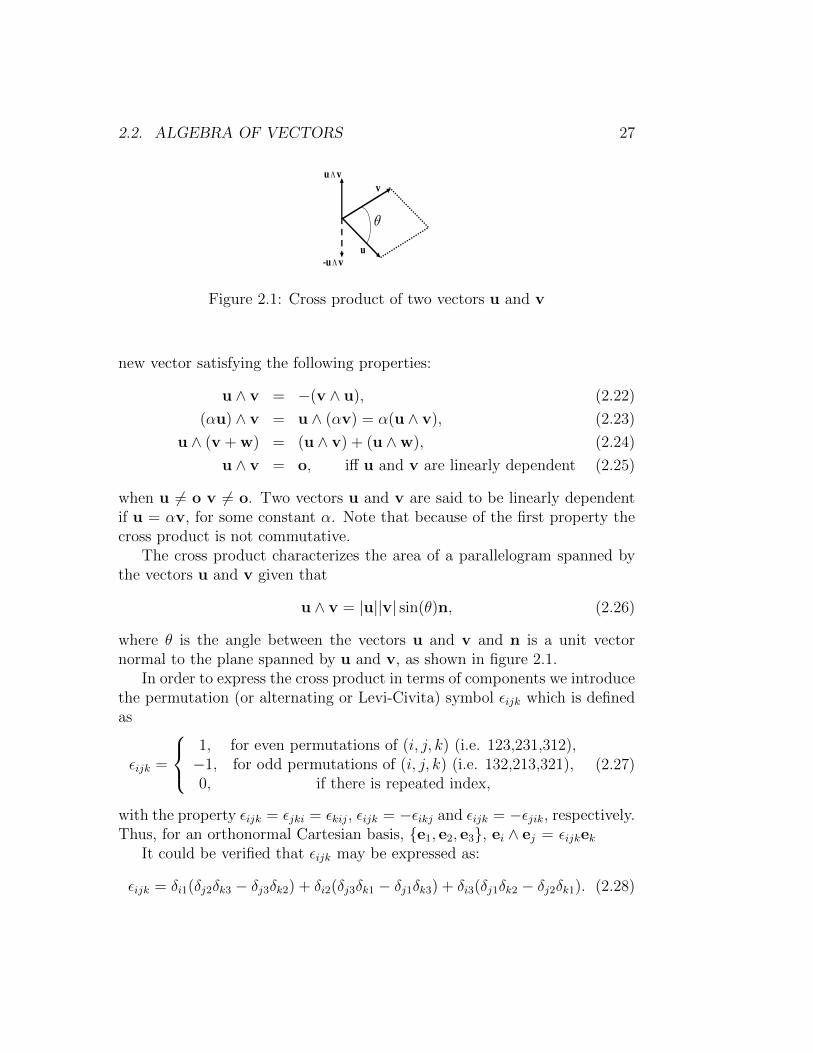
u ∧ v = |u||v| sin(θ)n, (2.26)
where θ is the angle between the vectors u and v and n is a unit vectornormal to the plane spanned by u and v, as shown in figure 2.1.
In order to express the cross product in terms of components we introducethe permutation (or alternating or Levi-Civita) symbol εijk which is definedas
εijk =
1, for even permutations of (i, j, k) (i.e. 123,231,312),−1, for odd permutations of (i, j, k) (i.e. 132,213,321),0, if there is repeated index,
(2.27)
with the property εijk = εjki = εkij, εijk = −εikj and εijk = −εjik, respectively.Thus, for an orthonormal Cartesian basis, e1, e2, e3, ei ∧ ej = εijkek
It could be verified that εijk may be expressed as:
εijk = δi1(δj2δk3 − δj3δk2) + δi2(δj3δk1 − δj1δk3) + δi3(δj1δk2 − δj2δk1). (2.28)
28 CHAPTER 2. MATHEMATICAL PRELIMINARIES
It could also be verified that the product of the permutation symbols εijkεpqris related to the Kronecker delta by the relation
εijkεpqr = δip(δjqδkr−δjrδkq)+δiq(δjrδkp−δjpδkr)+δir(δjpδkq−δjqδkp). (2.29)
We deduce from the above equation (2.29) the important relations:
εijkεpqk = δipδjq − δiqδjp, εijkεpjk = 2δip, εijkεijk = 6. (2.30)
The triple scalar (or box) product: [u,v,w] represents the volume V ofa parallelepiped spanned by u, v, w forming a right handed triad. Thus, inindex notation:
V = [u,v,w] = (u ∧ v) ·w = εijkuivjwk. (2.31)
Note that the vectors u, v, w are linearly dependent if and only if their scalartriple product vanishes, i.e., [u,v,w] = 0
The product (u ∧ v) ∧ w is called the vector triple product and it maybe verified that
(u ∧ v) ∧w = εkqr(εijkuivj)wqer = εqrkεijkuivjwqer (2.32)
= (δqiδrj − δqjδri)uivjwqer (2.33)
= (uqvrwq − urvqwq)er (2.34)
= (u ·w)v − (v ·w)u. (2.35)
Similarly, it can be shown that
u ∧ (v ∧w) = (u ·w)v − (u · v)w. (2.36)
Thus triple product, in general, is not associative, i.e., u∧(v∧w) 6= (u∧v)∧w.
2.3 Algebra of second order tensors
A second order tensor A, for our purposes here, may be thought of as a linearfunction that maps a directed line segment to another directed line segment.This we write as, v = Au where A is the linear function that assigns a vectorv to each vector u. Since A is a linear function,
A(αu + βv) = αAu + βAv, (2.37)
2.3. ALGEBRA OF SECOND ORDER TENSORS 29
for all vectors u, v and all scalars α, β.If A and B are two second order tensors, we can define the sum A + B,
the difference A − B and the scalar multiplication αA by the rules
(A±B)u = Au±Bu, (2.38)
(αA)u = α(Au), (2.39)
where u denotes an arbitrary vector. The important second order unit (oridentity) tensor 1 and the second order zero tensor 0 are defined, respectively,by the relation 1u = u and 0u = o, for all (∀) vectors u.
If the relation v · Av ≥ 0 holds for all vectors, then A is said to be apositive semi-definite tensor. If the condition v ·Av > 0 holds for all nonzerovectors v, then A is said to be positive definite tensor. Tensor A is callednegative semi-definite if v ·Av ≤ 0 and negative definite if v ·Av < 0 forall vectors, v 6= o, respectively.
The tensor (or direct or matrix) product or the dyad of the vectors u andv is denoted by u⊗ v. It is a second order tensor which linearly transformsa vector w into a vector with the direction of u following the rule
(u⊗ v)w = (v ·w)u. (2.40)
The dyad satisfies the linearity property
(u⊗ v)(αw + βx) = α(u⊗ v)w + β(u⊗ v)x. (2.41)
The following relations are easy to establish:
(αu + βv)⊗w = α(u⊗w) + β(v ⊗w), (2.42)
(u⊗ v)(w ⊗ x) = (v ·w)(u⊗ x), (2.43)
A(u⊗ v) = (Au)⊗ v, (2.44)
where, A is an arbitrary second order tensor, u, v, w and x are arbitraryvectors and α and β are arbitrary scalars. Dyad is not commutative, i.e.,u⊗ v 6= v ⊗ u and (u⊗ v)(w ⊗ x) 6= (w ⊗ x)(u⊗ v).
A dyadic is a linear combination of dyads with scalar coefficients, forexample, α(u ⊗ v) + β(w ⊗ x). Any second-order tensor can be expressedas a dyadic. As an example, the second order tensor A may be representedby a linear combination of dyads formed by the Cartesian basis ei, i.e.,
30 CHAPTER 2. MATHEMATICAL PRELIMINARIES
A = Aijei ⊗ ej. The nine Cartesian components of A with respect to ei,represented by Aij can be expressed as a matrix [A], i.e.,
[A] =
A11 A12 A13
A21 A22 A23
A31 A32 A33
. (2.45)
This is known as the matrix notation of tensor A. We call A, which isresolved along basis vectors that are orthonormal and fixed, a Cartesiantensor of order two. Then, the components of A with respect to a fixed,orthonormal basis vectors ei is obtained as:
Aij = ei ·Aej. (2.46)
The Cartesian components of the unit tensor 1 form the Kronecker deltasymbol, thus 1 = δijei ⊗ ej = ei ⊗ ei and in matrix form
1 =
1 0 00 1 00 0 1
(2.47)
Next we would like to derive the components of u⊗v along an orthonor-mal basis ei. Using the representation (2.46) we find that
(u⊗ v)ij = ei · (u⊗ v)ej
= (ei · u)(ej · v)
= uivj, (2.48)
where ui and vj are the Cartesian components of the vectors u and v re-spectively. Writing the above equation in the convenient matrix notation wehave
(u⊗ v)ij =
u1
u2
u3
[ v1 v2 v3
]=
u1v1 u1v2 u1v3
u2v1 u2v2 u2v3
u3v1 u3v2 u3v3
. (2.49)
The product of two second order tensors A and B, denoted by AB,is again a second order tensor. It follows from the requirement (AB)u =A(Bu), for all vectors u.
2.3. ALGEBRA OF SECOND ORDER TENSORS 31
Further, the product of second order tensors is not commutative, i.e., AB6= BA. The components of the product AB along an orthonormal basis eiis found to be:
(AB)ij = ei · (AB)ej = ei ·A(Bej), (2.50)
= ei ·A(Bkjek) = (ei ·Aek)Bkj, (2.51)
= AikBkj. (2.52)
The following properties hold for second order tensors:
A + B = B + A, (2.53)
A + 0 = A, (2.54)
A + (−A) = 0, (2.55)
(A + B) + C = A + (B + C), (2.56)
(AB)C = A(BC) = ABC, (2.57)
A2 = AA, (2.58)
(A + B)C = AC + BC, (2.59)
Note that the relations AB = 0 and Au = o does not imply that A orB is 0 or u = o.
The unique transpose of a second order tensor A denoted by At is gov-erned by the identity:
v ·Atu = u ·Av (2.60)
for all vectors u and v.Some useful properties of the transpose are
(At)t = A, (2.61)
(αA + βB)t = αAt + βBt, (2.62)
(AB)t = BtAt, (2.63)
(u⊗ v)t = v ⊗ u. (2.64)
From identity (2.60) we obtain ei ·Atej = ej ·Aei, which gives, in regardto equation (2.46), the relation (At)ij = Aji.
The trace of a tensor A is a scalar denoted by tr(A) and is defined as:
tr(A) =[Au,v,w] + [u,Av,w] + [u,v,Aw]
[u,v,w](2.65)

32 CHAPTER 2. MATHEMATICAL PRELIMINARIES
where u, v, w are any vectors such that [u,v,w] 6= 0, i.e., these vectorsspan the entire 3D vector space. Thus, tr(m⊗ n) = m · n. Let us see how:Without loss of generality we can assume the vectors u, v and w to be m,n and (m ∧ n) respectively. Then, (2.65) becomes
tr(m⊗ n) =(n ·m)[m,n,m ∧ n] + |n|[m,m,m ∧ n] + [m,n,n][m,n,m]
[m,n,m ∧ n],
= n ·m. (2.66)
The following properties of trace is easy to establish from (2.65):
tr(At) = tr(A), (2.67)
tr(AB) = tr(BA), (2.68)
tr(αA + βB) = αtr(A) + βtr(B). (2.69)
Then, the trace of a tensor A with respect to the orthonormal basis ei isgiven by
tr(A) = tr(Aijei ⊗ ej) = Aijtr(ei ⊗ ej)
= Aijei · ej = Aijδij = Aii
= A11 + A22 + A33 (2.70)
The dot product between two tensors denoted by A ·B, just like the dotproduct of two vectors yields a real value and is defined as
A ·B = tr(AtB) = tr(BtA) (2.71)
Next, we record some useful properties of the dot operator:
1 ·A = tr(A) = A · 1, (2.72)
A · (BC) = BtA ·C = ACt ·B, (2.73)
A · (u⊗ v) = u ·Av, (2.74)
(u⊗ v) · (w ⊗ x) = (u ·w)(v · x). (2.75)
Note that if we have the relation A·B = C·B, in general, we cannot concludethat A equals C. A = C only if the above equality holds for any arbitraryB.
The norm of a tensor A is denoted by |A| (or ‖A‖). It is a non-negativereal number and is defined by the square root of A ·A, i.e.,
|A| = (A ·A)1/2 = (AijAij)1/2. (2.76)
2.3. ALGEBRA OF SECOND ORDER TENSORS 33
The determinant of a tensor A is defined as:
det(A) =[Au,Av,Aw]
[u,v,w], (2.77)
where u, v, w are any vectors such that [u,v,w] 6= 0, i.e., these vectors spanthe entire 3D vector space. In index notation:
det(A) = εijkAi1Aj2Ak3. (2.78)
Then, it could be shown that
det(AB) = det(A) det(B), (2.79)
det(At) = det(A). (2.80)
A tensor A is said to be singular if and only if det(A) = 0. If A is anon-singular tensor i.e., det(A) 6= 0, then there exist a unique tensor A−1,called the inverse of A satisfying the relation
AA−1 = A−1A = 1. (2.81)
If tensors A and B are invertible (i.e., they are non-singular), then the prop-erties
(AB)−1 = B−1A−1, (2.82)
(A−1)−1 = A, (2.83)
(αA)−1 =1
αA−1, (2.84)
(A−1)t = (At)−1 = A−t, (2.85)
A−2 = A−1A−1, (2.86)
det(A−1) = (det(A))−1, (2.87)
hold.Corresponding to an arbitrary tensor A there is a unique tensor A∗, called
the adjugate of A, such that
A∗(a ∧ b) = Aa ∧Ab, (2.88)
for any arbitrary vectors a and b in the vector space. Suppose that A isinvertible and that a, b, c are arbitrary vectors, then
At∗(a ∧ b) · c = [Ata,Atb,AtA−tc]
= det(At)(a ∧ b) · A−tc= det(A)A−1(a ∧ b) · c, (2.89)

34 CHAPTER 2. MATHEMATICAL PRELIMINARIES
where successive use has been made of equations (2.88), (2.81), (2.63), (2.77)and (2.60). Because of the arbitrariness of a, b, c there follows the connection
A−1 =1
det(A)At∗, (2.90)
between the inverse of A and the adjugate of At.
2.3.1 Orthogonal tensor
An orthogonal tensor Q is a linear function satisfying the condition
Qu ·Qv = u · v, (2.91)
for all vectors u and v. As can be seen, the dot product is invariant (its valuedoes not change) due to the transformation of the vectors by the orthogonaltensor. The dot product being invariant means that both the angle, θ betweenthe vectors u and v and the magnitude of the vectors |u|, |v| are preserved.Consequently, the following properties of orthogonal tensor can be inferred:
QQt = QtQ = 1, (2.92)
det(Q) = ±1. (2.93)
It follows from (2.92) that Q−1 = Qt. If det(Q) = 1, Q is said to be properorthogonal tensor and this transformation corresponds to a rotation. On theother hand, if det(Q) = −1, Q is said to be improper orthogonal tensor andthis transformation corresponds to a reflection superposed on a rotation.
Figure 2.2 shows what happens to two directed line segments, u1 andv1 under the action the two kinds of orthogonal tensors. A proper orthogo-nal tensor corresponding to a rotation about the e3 basis, whose Cartesiancoordinate components are given by
Q =
cos(α) sin(α) 0− sin(α) cos(α) 0
0 0 1
, (2.94)
transforms, u1 to u+1 and v1 to v+
1 , maintaining their lengths and the anglebetween these line segments. Here α = Φ − Θ. An improper orthogonal

2.3. ALGEBRA OF SECOND ORDER TENSORS 35
u 1+
e1
e₂
u 1
v 1
v 1+
u 1-
v 1-
Figure 2.2: Schematic of transformation of directed line segments u1 and v1
under the action of proper orthogonal tensor to u+1 and v+
1 as well as byimproper orthogonal tensor to u−1 and v−1 respectively.
tensor corresponding to reflection about e1 axis, whose Cartesian coordinatecomponents are given by
Q =
−1 0 00 1 00 0 1
, (2.95)
transforms, u1 to u−1 and v1 to v−1 , still maintaining their lengths and theangle between these line segments a constant.
2.3.2 Symmetric and skew tensors
A symmetric tensor, S and a skew symmetric tensor, W are such:
S = St or Sij = Sji, W = −Wt or Wij = −Wji, (2.96)
therefore the matrix components of these tensor reads
[S] =
S11 S12 S13
S12 S22 S23
S13 S23 S33
, [W] =
0 W12 W13
−W12 0 W23
−W13 −W23 0
, (2.97)
36 CHAPTER 2. MATHEMATICAL PRELIMINARIES
thus, there are only six independent components in symmetric tensors andthree independent components in skew tensors. Since, there are only threeindependent scalar quantities that in a skew tensor, it behaves like a vectorwith three components. Indeed, the relation holds:
Wu = ω ∧ u, (2.98)
where u is any vector and ω characterizes the axial (or dual) vector of theskew tensor W, with the property |ω| = |W|/
√2 (proof is omitted). The
relation between the Cartesian components of W and ω is obtained as:
Wij = ei ·Wej = ei · (ω ∧ ej) = ei · (ωkek ∧ ej)
= ei · (ωkεkjlel) = ωkεkjlδil
= εkjiωk = −εijkωk. (2.99)
Thus, we get
W12 = −ε12kωk = −ω3, (2.100)
W13 = −ε13kωk = ω2, (2.101)
W23 = −ε23kωk = −ω1, (2.102)
where the components W12, W13, W23 form the entries of the matrix [W] ascharacterized in (2.97)b.
Any tensor A can always be uniquely decomposed into a symmetric ten-sor, denoted by S (or sym(A)), and a skew (or antisymmetric) tensor, de-noted by W (or skew(A)). Hence, A = S + W, where
S =1
2(A + At), W =
1
2(A−At) (2.103)
Next, we shall look at some properties of symmetric and skew tensors:
S ·B = S ·Bt = S · 1
2(B + Bt), (2.104)
W ·B = −W ·Bt = W · 1
2(B−Bt), (2.105)
S ·W = W · S = 0, (2.106)
where B denotes any second order tensor. The first of these equalities in theabove equations is due to the property of the dot and trace operator, namelyA ·B = At ·Bt and that A ·B = B ·A.

2.3. ALGEBRA OF SECOND ORDER TENSORS 37
2.3.3 Projection tensor
Consider any vector u and a unit vector e. Then, we write u = u‖ + u⊥,with u‖ and u⊥ characterizing the projection of u onto the line spanned by eand onto the plane normal to e respectively. Using the definition of a tensorproduct (2.40) we deduce that
u‖ = (u · e)e = (e⊗ e)u = P‖eu, (2.107)
u⊥ = u− u‖ = u− (e⊗ e)u = (1− e⊗ e)u = P⊥e u, (2.108)
where
P‖e = e⊗ e, (2.109)
P⊥e = 1− e⊗ e, (2.110)
are projection tensors of order two. A tensor P is a projection if P is sym-metric and Pn = P where n is a positive integer, with properties:
P‖e + P⊥e = 1, (2.111)
P‖eP‖e = P‖e, (2.112)
P⊥e P⊥e = P⊥e , (2.113)
P‖eP⊥e = 0. (2.114)
2.3.4 Spherical and deviatoric tensors
Any tensor of the form α1, with α denoting a scalar is known as a sphericaltensor.
Every tensor A can be decomposed into its so called spherical part andits deviatoric part, i.e.,
A = α1 + dev(A), or Aij = αδij + [dev(A)]ij, (2.115)
where α = tr(A)/3 = Aii/3 and dev(A) is known as a deviator of A or adeviatoric tensor and is defined as dev(A) = A − (1/3)tr(A)1, or [dev(A)]ij= Aij − (1/3)Akkδij. It then can be easily verified that tr(dev(A)) = 0, forany second order tensor A.

38 CHAPTER 2. MATHEMATICAL PRELIMINARIES
2.3.5 Polar Decomposition theorem
Above we saw two additive decompositions of an arbitrary tensor A. Of com-parable significance in continuum mechanics are the multiplicative decompo-sitions afforded by the polar decomposition theorem. This result states thatan arbitrary invertible tensor A can be uniquely expressed in the forms
A = QU = VQ, (2.116)
where Q is an orthogonal tensor and U, V are positive definite symmetrictensors. It should be noted that Q is proper or improper orthogonal accordingas det(A) is positive or negative. (See, for example, Chadwick [1] for proofof the theorem.)
2.4 Algebra of fourth order tensors
A fourth order tensor A may be thought of as a linear function that mapssecond order tensor A into another second order tensor B. While this istoo narrow a viewpoint1, it suffices for the study of mechanics. We write B= A : A which defines a linear transformation that assigns a second ordertensor B to each second order tensor A.
We can express any fourth order tensor, A in terms of the three Cartesianbasis vectors as
A = Aijklei ⊗ ej ⊗ ek ⊗ el, (2.117)
where Aijkl are the Cartesian components of A. Thus, the fourth order tensorA has 34 = 81 components. Remember that any repeated index has to besummed from one through three.
One example for a fourth order tensor is the tensor product of the fourvectors u, v, w, x, denoted by u⊗ v⊗w⊗ x. We have the useful property:
(u⊗ v)⊗ (w ⊗ x) = u⊗ v ⊗w ⊗ x. (2.118)
If A = u⊗ v ⊗w ⊗ x, then it is easy to see that the Cartesian componentsof A, Aijkl = uivjwkxl, where ui, vj, wk, xl are the Cartesian components ofthe vectors u, v, w and x respectively.
1A fourth order tensor can operate on a vector to yield third order tensor or can operateon a third order tensor to yield an vector.

2.4. ALGEBRA OF FOURTH ORDER TENSORS 39
Another example of a fourth order tensor, is the tensor obtained from thetensor product of two second order tensors, i.e., D = A⊗B, where A, B aresecond order tensors and D is the fourth order tensor. In index notation wemay write: Dijkl = AijBkl where Dijkl, Aij, Bkl are the Cartesian componentsof the respective tensors.
The double contraction of a fourth order tensor A with a second ordertensor B results in a second order tensor, denoted by A : B with the propertythat:
(u⊗ v ⊗w ⊗ x) : (y ⊗ z) = (w · y)(x · z)(u⊗ v), (2.119)
(y ⊗ z) : (u⊗ v ⊗w ⊗ x) = (u · y)(v · z)(w ⊗ x). (2.120)
Hence, we can show that the components of A, Aijkl can be expressed as
Aijkl = (ei ⊗ ej) · A : (ek ⊗ el) = (ei ⊗ ej) : A · (ek ⊗ el) (2.121)
Next, we compute the Cartesian components of A : B to be:
A : B = AijklBmn(ei ⊗ ej ⊗ ek ⊗ el) : (em ⊗ en)
= AijklBmnδkmδlnei ⊗ ej
= AijklBklei ⊗ ej, (2.122)
where Aijkl and Bmn are the Cartesian components of the tensors A and B.Note that B : A 6= A : B.
Then, the following can be established:
(A⊗B) : C = (B ·C)A, (2.123)
A : (B⊗C) = (A ·B)C, (2.124)
where A, B, C and D are second order tensors.The unique transpose of a fourth order tensor A denoted by At is governed
by the identityB · At : C = C · A : B = A : B ·C (2.125)
for all the second order tensors B and C. From the above identity we deducethe index relation (At)ijkl = Aklij. The following properties of fourth ordertensors can be established:
(At)t = A, (2.126)
(A⊗B)t = B⊗A. (2.127)
40 CHAPTER 2. MATHEMATICAL PRELIMINARIES
Next, we define fourth order unit tensors I and I so that
A = I : A, At = I : A, (2.128)
for any second order tensor A. These fourth order unit tensors may berepresented by
I = δikδjlei ⊗ ej ⊗ ek ⊗ el = ei ⊗ ej ⊗ ei ⊗ ej, (2.129)
I = δilδjkei ⊗ ej ⊗ ek ⊗ el = ei ⊗ ej ⊗ ej ⊗ ei, (2.130)
where (I)ijkl = δikδjl and (I)ijkl = δilδjk define the Cartesian components ofI and I, respectively. Note that I 6= It.
The deviatoric part of a second order tensor A may be described by meansof a fourth order projection tensor, P where
dev(A) = P : A, P = I− 1
31⊗ 1. (2.131)
Thus the components of dev(A) and A are related through the expression[dev(A)]ij = PijklAkl, with Pijkl = δikδjl − (1/3)δijδkl.
Similarly, the fourth order tensors S and W given by
S =1
2(I + I), W =
1
2(I− I), (2.132)
are such that for any second order tensor A, they assign symmetric and skewpart of A respectively, i.e.,
S : A =1
2(A + At), W : A =
1
2(A−At). (2.133)
2.4.1 Alternate representation for tensors
Till now, we represented second order tensor components in a matrix form,for the advantages that it offers in computing other quantities and definingother operators. However, when we want to study mapping of second or-der tensor on to another second order tensor, this representation seem to beinconvenient. For this purpose, we introduce this alternate representation.Now, we view the second order tensor as a column vector of nine components

2.5. EIGENVALUES, EIGENVECTORS OF TENSORS 41
instead of a 3 by 3 matrix as introduced in (2.45). The order of these com-ponents is subjective. Keeping in mind the application of this is to studyelasticity, we order the components of a general second order tensor, A, as,
A =
A11
A22
A33
A12
A13
A21
A23
A31
A32
. (2.134)
In view of this, the fourth order tensor, which for us is a linear functionthat maps a second order tensor to another second order tensor, can berepresented as a 9 by 9 matrix as,
Bi =9∑j=1
[C]ijAj, i = 1 . . . 9. (2.135)
where A and B are second order tensors and C is a fourth order tensor. Notethat as before the fourth order tensor has 81 (=9*9) components. Thus, nowthe fourth order tensor is a matrix which is the reason for representing thesecond order tensor as vector.
2.5 Eigenvalues, eigenvectors of tensors
The scalar λi characterize eigenvalues (or principal values) of a tensor A ifthere exist corresponding nonzero normalized eigenvectors ni (or principaldirections or principal axes) of A, so that
Ani = λini, (i = 1,2,3; no summation). (2.136)
To identify the eigenvectors of a tensor, we use subsequently a hat on thevector quantity concerned, for example, n.
Thus, a set of homogeneous algebraic equations for the unknown eigen-values λi, i = 1,2,3, and the unknown eigenvectors ni, i = 1,2,3, is
(A− λi1)ni = o, (i = 1,2,3; no summation). (2.137)
42 CHAPTER 2. MATHEMATICAL PRELIMINARIES
For the above system to have a solution ni 6= o the determinant of the systemmust vanish. Thus,
det(A− λi1) = 0 (2.138)
where
det(A− λi1) = −λ3i + I1λ
2i − I2λi + I3. (2.139)
This requires that we solve a cubic equation in λ, usually written as
λ3 − I1λ2 + I2λ− I3 = 0, (2.140)
called the characteristic polynomial (or equation) for A, the solutions ofwhich are the eigenvalues λi, i = 1,2,3. Here, Ii, i = 1,2,3, are the so-calledprincipal scalar invariants of A and are given by
I1 = tr(A) = Aii = λ1 + λ2 + λ3,
I2 =1
2[(tr(A))2 − tr(A2)] =
1
2(AiiAjj − AmnAnm) = λ1λ2 + λ2λ3 + λ1λ3,
I3 = det(A) = εijkAi1Aj2Ak3 = λ1λ2λ3. (2.141)
If A is invertible then we can compute I2 using the expression I2 = tr(A−1)det(A).
A repeated application of tensor A to equation (2.136) yields Aαni =λαi ni, i = 1,2,3, for any positive integer α. (If A is invertible then α canbe any integer; not necessarily positive.) Using this relation and (2.140)multiplied by ni, we obtain the well-known Cayley-Hamilton equation:
A3 − I1A2 + I2A− I31 = 0. (2.142)
It states that every second order tensor A satisfies its own characteristicequation. As a consequence of Cayley-Hamilton equation, we can expressAα in terms of A2, A, 1 and principal invariants for positive integer, α >2. (If A is invertible, the above holds for any integer value of α positive ornegative provided α 6= 0, 1, 2.)
For a symmetric tensor S the characteristic equation (2.140) always hasthree real solutions and the set of eigenvectors form a orthonormal basisni (the proof of this statement is omitted). Hence, for a positive definitesymmetric tensor A, all eigenvalues λi are (real and) positive since, using(2.136), we have λi = ni ·Ani > 0, i = 1,2,3.

2.5. EIGENVALUES, EIGENVECTORS OF TENSORS 43
Any symmetric tensor S may be represented by its eigenvalues λi, i =1,2,3, and the corresponding eigenvectors of S forming an orthonormal basisni. Thus, S can be expressed as
S =3∑i=1
λini ⊗ ni, (2.143)
called the spectral representation (or spectral decomposition) of S. Thus,when orthonormal eigenvectors are used as the Cartesian basis to representS then
[S] =
λ1 0 00 λ2 00 0 λ3
. (2.144)
The above holds when all the three eigenvalues are distinct. On the otherhand, if there exists a pair of equal roots, i.e., λ1 = λ2 = λ 6= λ3, with anunique eigenvector n3 associated with λ3, we deduce that
S = λ3(n3 ⊗ n3) + λ[1− (n3 ⊗ n3)] = λ3P‖n3
+ λP⊥n3, (2.145)
where P‖n3
and P⊥n3denote projection tensors introduced in (2.109) and
(2.110) respectively. Finally, if all the three eigenvalues are equal, i.e., λ1
= λ2 = λ3 = λ, thenS = λ1, (2.146)
where every direction is a principal direction and every set of mutually or-thogonal basis denotes principal axes.
It is important to recognize that eigenvalues characterize the physicalnature of the tensor and that they do not depend on the coordinates chosen.
2.5.1 Square root theorem
Let C be symmetric and positive definite tensor. Then there is a uniquepositive definite, symmetric tensor U such that
U2 = C. (2.147)
We write√
C for U. If spectral representation of C is:
C =3∑i=1
λini ⊗ ni, (2.148)
44 CHAPTER 2. MATHEMATICAL PRELIMINARIES
then the spectral representation for U is:
U =3∑i=1
√λini ⊗ ni, (2.149)
where we have assumed that the eigenvalues of C, λi are distinct. On theother hand if λ1 = λ2 = λ3 = λ then
U =√λ1. (2.150)
If λ1 = λ2 = λ 6= λ3, with an unique eigenvector n3 associated with λ3 then
U =√λ3(n3 ⊗ n3) +
√λ[1− (n3 ⊗ n3)] (2.151)
(For proof of this theorem, see for example, Gurtin [2].)
2.6 Transformation laws
Consider two sets of mutually orthogonal basis vectors which share a com-mon origin. They correspond to a ‘new’ and an ‘old’ (original) Cartesiancoordinate system which we assume to be right-handed characterized by twosets of basis vectors ei and ei, respectively. Hence, the new coordinatesystem could be obtained from the original one by a rotation of the basisvectors ei about their origin. We then define the directional cosine matrix,Qij, as,
Qij = ei · ej = cos(θ(ei, ej)). (2.152)
Note that the first index on Qij indicates the ‘old’ components whereas thesecond index holds for the ‘new’ components.
It is worthwhile to mention that vectors and tensors themselves remaininvariant upon a change of basis - they are said to be independent of thecoordinate system. However, their respective components do depend uponthe coordinate system introduced. This is the reason why a set of numbersarranged as a 3 by 1 or 3 by 3 matrix is not a vector or a tensor.
2.6.1 Vectorial transformation law
Consider some vector u represented using the two sets of basis vectors eiand ei, i.e.,
u = uiei = uj ej. (2.153)

2.6. TRANSFORMATION LAWS 45
Recalling the method to find the components of the vector along the basisdirections, (2.15),
uj = u · ej = (uiei) · ej = Qijui, (2.154)
from the definition of the directional cosine matrix, (2.152). We assume thatthe relation between the basis vectors ei and ej is known and hence giventhe components of a vector in a basis, its components in another basis canbe found using equation (2.154).
In an analogous manner, we find that
uj = u · ej = (uiei) · ej = Qjiui. (2.155)
The results of equations (2.154) and (2.155) could be cast in matrix notationas
[u] = [Q]t[u], and [u] = [Q][u], (2.156)
respectively. It is important to emphasize that the above equations are notidentical to u = Qtu and u = Qu, respectively. In (2.156) [u] and [u]are column vectors characterizing components of the same vector in twodifferent coordinate systems, whereas u and u are different vectors, in thelater. Similarly, [Q] is a matrix of directional cosines, it is not a tensor eventhough it has the attributes of an orthogonal tensor as we will see next.
Combining equations (2.154) and (2.155), we obtain
uj = Qjiui = QjiQaiua, and uj = Qijui = QijQiaua (2.157)
Hence, (QaiQji − δja)ua = 0 and (QijQia − δja)ua = 0 for any vector u.Therefore,
QaiQji = δja, or [Q][Q]t = [1], (2.158)
QiaQij = δja, or [Q]t[Q] = [1]. (2.159)
Thus, the transformation matrix, Qij is sometimes called as orthogonal ma-trix but never as orthogonal tensor.
2.6.2 Tensorial transformation law
To determine the transformation laws for the Cartesian components of anysecond-order tensor A, we proceed along the lines similar to that done for

46 CHAPTER 2. MATHEMATICAL PRELIMINARIES
vectors. Since, we seek the components of the same tensor in two differentbasis,
A = Aabea ⊗ eb = Aijei ⊗ ej. (2.160)
Then it follows from (2.46) that,
Aij = ei ·Aej = ei · (Aabea ⊗ eb)ej
= Aab(eb · ej)(ea · ei) = AabQaiQbj. (2.161)
In matrix notation, [A] = [Q]t[A][Q]. In an analogous manner, we find that
Aij = QikQjmAkm, or [A] = [Q][A][Q]t. (2.162)
We emphasize again that these transformations relates the different matrices[A] and [A], which have the components of the same tensor A and the equa-tions [A] = [Q]t[A][Q] and [A] = [Q][A][Q]t differ from the tensor equationsA = QtAQ and A = QAQt, relating two different tensors, namely A andA.
Finally, the 3n components Aj1j2...jn of a tensor of order n (with n indicesj1, j2, . . ., jn) transform as
Ai1i2...in = Qj1i1Qj2i2 . . . QjninAj1j2...jn . (2.163)
This tensorial transformation law relates the different components Ai1i2...in(along the directions e1, e2, e3) and Aj1j2...jn (along the directions e1, e2, e3)of the same tensor of order n.
We note that, in general a second order tensor, A will be represented asAijei⊗Ej, where ei and Ej are different basis vectors spanning the samespace. It is not necessary that the directional cosines Qij = Ei · Ei and qij =ei · ei be the same, where ei and Ej are the ‘new’ basis vectors with respect towhich the matrix components of A is sought. Thus, generalizing the aboveis straightforward; each directional cosine matrices can be different, contraryto the assumption made.
2.6.3 Isotropic tensors
A tensor A is said to be isotropic if its components are the same underarbitrary rotations of the basis vectors. The requirement is deduced fromequation (2.161) as
Aij = QkiQmjAkm or [A] = [Q]t[A][Q]. (2.164)
2.7. SCALAR, VECTOR, TENSOR FUNCTIONS 47
Of course here we assume that the components of the tensor are with respectto a single basis and not two or more independent basis.
Note that all scalars, zeroth order tensors are isotropic tensors. Also, zerotensors and unit tensors of all orders are isotropic. It can be easily verifiedthat for second order tensors spherical tensor is also isotropic. The mostgeneral isotropic tensor of order four is of the form
α(1⊗ 1) + βI + γI, (2.165)
where α, β, γ are scalars. The same in component form is given by: αδijδkl+ βδikδjl + γδilδjk.
2.7 Scalar, vector, tensor functions
Having got an introduction to algebra of tensors we next focus on tensorcalculus. Here we shall understand the meaning of a function and definewhat we mean by continuity and derivative of a function.
A function is a mathematical correspondence that assigns exactly oneelement of one set to each element of the same or another set. Thus, ifwe consider scalar functions of one scalar variable, then for each element(value) in the subset of the real line one associates an element in the realline or in the space of vectors or in the space of second order tensors. Forexample, Φ = Φ(t), u = u(t) = ui(t)ei, A = A(t) = Aij(t)ei ⊗ ej are scalarvalued, vector valued, second order tensor valued scalar functions with a setof Cartesian basis vectors assumed to be fixed. The components ui(t) andAij(t) are assumed to be real valued smooth functions of t varying over acertain interval.
The first derivative of the scalar function Φ is simply Φ = dΦ/dt. Recol-lecting from a first course in calculus, dΦ/dt stands for that unique value ofthe limit
limh→0
Φ(t+ h)− Φ(t)
h(2.166)
The first derivative of u and A with respect to t (rate of change) de-noted by u = du/dt and A = dA/dt, is given by the first derivative of theirassociated components. Since, dei/dt = o, i = 1, 2, 3, we have
u = ui(t)ei, A = Aij(t)ei ⊗ ej. (2.167)
48 CHAPTER 2. MATHEMATICAL PRELIMINARIES
In general, the nth derivative of u and A (for any desired n) denoted bydnu/dtn and dnA/dtn, is a vector-valued and tensor-valued function whosecomponents are dnui/dt
n and dnAij/dtn, respectively. Again we have as-
sumed that dei/dt = o.By applying the rules of differentiation, we obtain the identities:
˙u± v = u± v, (2.168)
Φu = Φu + Φu, (2.169)˙u⊗ v = u⊗ v + u⊗ v, (2.170)˙A±B = A± B, (2.171)
Au = Au + Au, (2.172)
At = At, (2.173)˙A ·B = A ·B + A · B, (2.174)
AB = AB + AB, (2.175)
where Φ is a scalar valued scalar function, u and v are vector valued scalarfunction, A and B are second order tensor valued scalar function. Here andelsewhere in this notes, the overbars cover the quantities to which the dotoperations are applied.
Since, AA−1 = 1,˙
AA−1 = 0. Hence, we compute:
˙A−1 = −A−1AA−1. (2.176)
A tensor function is a function whose arguments are one or more tensorvariables and whose values are scalars, vectors or tensors. The functionsΦ(B), u(B), and A(B) are examples of so-called scalar-valued, vector-valuedand second order tensor-valued functions of one second order tensor variableB, respectively. In an analogous manner, Φ(v), u(v), and A(v) are scalar-valued, vector-valued and second order tensor-valued functions of one vectorvariable v, respectively.
Let D denote the region of the vector space that is of interest. Then ascalar field Φ, defined on a domain D, is said to be continuous if
limα→0|Φ(v + αa)− Φ(v)| = 0, ∀v ∈ D, a ∈ V, (2.177)
where V denote the set of all vectors in the vector space. The properties ofcontinuity are attributed to a vector field u and a tensor field A defined onD, if they apply to the scalar field u · a and a ·Ab ∀ a and b ∈ V.
2.7. SCALAR, VECTOR, TENSOR FUNCTIONS 49
Consider a scalar valued function of one second order tensor variable A,Φ(A). Assuming the function Φ is continuous in A, the derivative of Φ withrespect to A, denoted by ∂Φ
∂A, is the second order tensor that satisfies
∂Φ
∂A·U =
d
ds[Φ(A + sU)] |s=0 = tr(
(∂Φ
∂A
)tU) = tr(
∂Φ
∂AUt), (2.178)
for any second order tensor U.Example: If Φ(A) = det(A), find ∂Φ
∂Aboth when A is invertible and
when it is not.Taking trace of the Cayley-Hamilton equation (2.142) and rearranging we
get
det(A) =1
6[2tr(A3)− 3tr(A)tr(A2) + (tr(A))3]. (2.179)
Hence,
∂[det(A)]
∂A=
1
6[2∂[tr(A3)]
∂A+3
∂[tr(A)]
∂A[(tr(A))2−tr(A2)]−3tr(A)
∂[tr(A2)]
∂A].
(2.180)Using the properties of trace and dot product we find that
tr(A + sU) = tr(A) + s1 ·U, (2.181)
tr([A + sU]2) = tr(A2) + 2sAt ·U + s2tr(U2), (2.182)
tr([A + sU]3) = tr(A3) + 3s(At)2 ·U + 3s2At ·U2 + s3tr(U3),(2.183)
from which, we deduce that
∂[tr(A)]
∂A= 1, (2.184)
∂[tr(A2)]
∂A= 2At, (2.185)
∂[tr(A3)]
∂A= 3(At)2, (2.186)
using equation (2.178). Substituting equations (2.184) through (2.186) in(2.180) we get
∂[det(A)]
∂A= (At)2 + I21− I1A
t. (2.187)
If A is invertible, then multiplying (2.142) by A−t and rearranging we get
(At)2 − I1At + I21 = I3A
−t. (2.188)

50 CHAPTER 2. MATHEMATICAL PRELIMINARIES
In light of the above equation, (2.187) reduces to
∂[det(A)]
∂A= det(A)A−t. (2.189)
Next, we consider a smooth tensor valued function of one second ordertensor variable A, f(A). As before, the derivative of f with respect to A,denoted by ∂f
∂A, is the fourth order tensor that satisfies
∂f
∂A: U =
d
ds[f(A + sU)] |s=0, (2.190)
for any second order tensor U.It is straight forward to see that when f(A) = A, where A is any second
order tensor, then (2.190) reduces to
∂f
∂A: U = U, (2.191)
hence, ∂f∂A
= I, the fourth order unit tensor where we have used equation(2.128a).
If f(A) = At where A is any second order tensor, then using (2.190) itcan be shown that ∂f
∂A= I obtained using equation (2.128b).
Now, say the tensor valued function f is defined only for symmetric ten-sors, and that f(S) = S, where S is a symmetric second order tensor. Com-pute the derivative of f with respect to S, i.e., ∂f
∂S.
First, since the function f is defined only for symmetric tensors, we haveto generalize the function for any tensor. This is required because U is anysecond order tensor. Hence, f(S) = f(1
2[A + At]) = f(A), where A is any
second order tensor. Now, find the derivative of f with respect to A and thenrewrite the result in terms of S. The resulting expression is the derivative off with respect to S. Hence,
f(A + sU) =1
2[A + At + s[U + Ut]]. (2.192)
Substituting the above in equation (2.190) we get
∂ f
∂A: U =
1
2[U + Ut]. (2.193)
Thus,∂ f
∂A=
1
2[I + I]. (2.194)
2.7. SCALAR, VECTOR, TENSOR FUNCTIONS 51
Consequently,∂f
∂S=
∂ f
∂A=
1
2[I + I]. (2.195)
Example - 1: Assume that A is an invertible tensor and f(A) = A−1.Then show that
∂f
∂A: U = −A−1UA−1. (2.196)
Recalling that all invertible tensors satisfy the relation AA−1 = 1, we obtain
(A + sU)(A + sU)−1 = 1. (2.197)
Differentiating the above equation with respect to s
U(A + sU)−1 + (A + sU)d
ds(A + sU)−1 = 0. (2.198)
Evaluating the above equation at s = 0, and rearranging
∂f
∂A: U =
d
ds(A + sU)−1|s=0 = −A−1UA−1. (2.199)
Hence proved.Example - 2: Assume that S is an invertible symmetrical tensor and
f(S) = S−1. Find ∂f∂S
.As before generalizing the given function, we have f(A) = 1
2[A+At]−1.
Following the same steps as in the previous example we obtain:
[A + At + s(U + Ut)][A + At + s(U + Ut)]−1 = 1. (2.200)
Differentiating the above equation with respect to s and evaluating at s = 0and rearranging we get
∂ f
∂A: U = 2
d
ds[A+At + s(U+Ut)]−1|s=0 = 2[A+At]−1[U+Ut][A+At]−1.
(2.201)Therefore,
∂f
∂S: U = −1
2S−1[U + Ut]S−1. (2.202)
Let Φ be a smooth scalar-valued function and A, B smooth tensor-valuedfunctions of a tensor variable C. Then, it can be shown that
∂(A ·B)
∂C= A :
∂B
∂C+ B :
∂A
∂C, (2.203)
∂(ΦA)
∂C= A⊗ ∂Φ
∂C+ Φ
∂A
∂C. (2.204)

52 CHAPTER 2. MATHEMATICAL PRELIMINARIES
2.8 Gradients and related operators
In this section, we consider scalar and vector-valued functions that assign ascalar and vector to each element in the subset of the set of position vectorsfor the points in 3D space. If x denotes the position vector of points in the3D space, then Φ(x) is a function that assigns a scalar Φ to each point inthe 3D space of interest and Φ is called the scalar field. A few examples ofscalar fields are temperature, density, energy. Similarly, the vector field u(x)assigns a vector to each point in the 3D space of interest. Displacement,velocity, acceleration are a few examples of vector fields.
Let D denote the region of the 3D space that is of interest, that is theset of position vectors of points that is of interest in the 3D space. Then ascalar field Φ, defined on a domain D, is said to be continuous if
limα→0|Φ(x + αa)− Φ(x)| = 0, ∀x ∈ D, a ∈ E, (2.205)
where E denote the set of all position vectors of points in the 3D space anda is a constant vector. The scalar field Φ is said to be differentiable if thereexist a vector field w such that
limα→0|w(x) · a− α−1[Φ(x + αa)− Φ(x)]| = 0, ∀x ∈ D, a ∈ E. (2.206)
It can be shown that there is at most one vector field, w satisfying the aboveequation (proof omitted). This unique vector field w is called the gradientof Φ and denoted by grad(Φ).
The properties of continuity and differentiability are attributed to a vectorfield u and a tensor field T defined on D, if they apply to the scalar field u ·aand a · Tb ∀ a and b ∈ E. Given that the vector field u, is differentiable,the gradient of u denoted by grad(u), is the tensor field defined by
grad(u)ta = grad(u · a) ∀a ∈ E (2.207)
The divergence and the curl of a vector u denoted as div(u) and curl(u), arerespectively scalar valued and vector valued and are defined by
div(u) = tr(grad(u)), (2.208)
curl(u) · a = div(u ∧ a), ∀a ∈ E. (2.209)
When the tensor field T is differentiable, its divergence denoted by div(T),is the vector field defined by
div(T) · a = div(Ta), ∀a ∈ E. (2.210)

2.8. GRADIENTS AND RELATED OPERATORS 53
If grad(Φ) exist and is continuous, Φ is said to be continuously differen-tiable and this property extends to u and T if grad(u · a) and grad(a ·Tb)exist and are continuous for all a, b ∈ E.
An important identity: For a continuously differentiable vector field, u
div((grad(u))t) = grad(div(u)). (2.211)
(Proof omitted)Let Φ and u be some scalar and vector field respectively. Then, the
Laplacian operator, denoted by ∆ (or by ∇2), is defined as
∆(Φ) = div(grad(Φ)), ∆(u) = div(grad(u)). (2.212)
The Hessian operator, denoted by ∇∇ is defined as
∇∇(Φ) = grad(grad(Φ)) (2.213)
If a vector field u is divergence free (i.e. div(u) = 0) then it is calledsolenoidal. It is called irrotational if curl(u) = o. It can be establishedthat
curl(curl(u)) = grad(div(u))−∆(u). (2.214)
Consequently, if a vector field, u is both solenoidal and irrotational, then∆(u) = o (follows from the above equation) and such a vector field is saidto be harmonic. If a scalar field Φ satisfies ∆(Φ) = 0, then Φ is said to beharmonic.
Potential theorem: Let u be a smooth point field on an open or closedsimply connected region R and let curl(u) = o. Then there is a continuouslydifferentiable scalar field on R such that
u = grad(Φ) (2.215)
From the definition of grad (2.207), it can be seen that it is a linearoperator. That is,
grad(u1 + u2) = grad(u1) + grad(u2). (2.216)
Consequently, all other operators div, ∆ are also linear operators.Before concluding this section we collect a few identities that are useful
subsequently. Here Φ, Ψ are scalar fields, u, v are vector fields and A is
54 CHAPTER 2. MATHEMATICAL PRELIMINARIES
second order tensor field.
div(Φu) = Φdiv(u) + u · grad(Φ), (2.217)
div(ΦA) = Φdiv(A) + Atgrad(Φ), (2.218)
div(Atu) = div(A) · u + A · grad(u), (2.219)
div(u ∧ v) = v · curl(u)− u · curl(v), (2.220)
div(u⊗ v) = (grad(u))v + div(v)u, (2.221)
grad(ΦΨ) = Ψgrad(Φ) + Φgrad(Ψ), (2.222)
grad(Φu) = u⊗ grad(Φ) + Φgrad(u), (2.223)
grad(u · v) = (grad(u))tv + (grad(v))tu, (2.224)
curl(Φu) = grad(Φ) ∧ u + Φcurl(u), (2.225)
curl(u ∧ v) = udiv(v)− vdiv(u) + (grad(u))v − (grad(v))u,(2.226)
∆(u · v) = v ·∆(u) + 2grad(u) · grad(v) + u ·∆(v). (2.227)
Till now, in this section we defined all the quantities in closed form butwe require them in component form to perform the actual calculations. Thiswould be the focus in the reminder of this section. In the following, let eidenote the Cartesian basis vectors and xi i = 1, 2, 3, the Cartesian coordi-nates.
Let Φ be differentiable scalar field, then it follows from equation (2.206),on replacing a by the base vectors ei in turn, that the partial derivatives ∂Φ
∂xi
exist in D and that, moreover, wi = ∂Φ∂xi
. Hence
grad(Φ) =∂Φ
∂xiei. (2.228)
Let u be differentiable vector field in D and a some constant vector in E.Then, using (2.228) we compute
grad(u·a) =∂(u · a)
∂xiei =
∂up∂xi
apei =∂up∂xi
eia·ep =
(∂up∂xi
ei ⊗ ep
)a, (2.229)
where ap and up are the Cartesian components of a and u respectively. Con-sequently, appealing to definition (2.207) we obtain
grad(u) =∂up∂xi
ep ⊗ ei. (2.230)

2.8. GRADIENTS AND RELATED OPERATORS 55
Then, according to the definition for divergence, (2.208)
div(u) =∂up∂xp
. (2.231)
Next, we compute div(u ∧ a) to be
div(u ∧ a) = ±∂(εijkuiaj)
∂xk= ±εijk
∂ui∂xk
aj = ±(εijk
∂ui∂xk
ej
)· (epap), (2.232)
using (2.231). Comparing the above result with the definition of curl in(2.209) we infer
curl(u) = ±εijk∂ui∂xk
ej (2.233)
Finally, let T be a differentiable tensor field in D, then we compute
div(Ta) =∂Tijaj∂xi
=∂Tij∂xi
aj =
(∂Tij∂xi
ej
)· (apep), (2.234)
using equation (2.231). Then, we infer
div(T) =∂Tij∂xi
ej, (2.235)
from the definition (2.210).The component form for the other operators, namely Laplacian and Hes-
sian can be obtained as
∆(Φ) =∂2Φ
∂x2i
, ∆(u) =∂2uj∂x2
i
ej, sum i from 1 to 3,(2.236)
∇∇(Φ) =∂2Φ
∂xi∂xjei ⊗ ej, (2.237)
respectively.Above we obtained the components of the different operators in Cartesian
coordinate system, we shall now proceed to obtain the same with respect toother coordinate systems. While using the method illustrated here we couldobtain the components in any orthogonal curvilinear system, we choose thecylindrical polar coordinate system for illustration.
56 CHAPTER 2. MATHEMATICAL PRELIMINARIES
First, we outline a general procedure to find the basis vectors for a givenorthogonal curvilinear coordinates. A differential vector dp in the 3D vec-tor space is written as dp = dxiei relative to Cartesian coordinates. Thesame coordinate independent vector in orthogonal curvilinear coordinates iswritten as
dp =∂p
∂xidxi =
∂p
∂zidzi, (2.238)
where zi denotes curvilinear coordinates. But
dp = dxiei = dzigi, (2.239)
where gi is the basis vectors in the orthogonal curvilinear coordinates. Thus,
ei =∂p
∂xi, and gi =
∂p
∂zi. (2.240)
Comparing equations (2.239) and (2.240) we obtain the desired transforma-tion relation between the bases to be:
gi =∂p
∂zi=
∂p
∂xk
∂xk∂zi
=∂xk∂zi
ek (2.241)
The basis gi so obtained will vary from point to point in the Euclidean spaceand will be orthogonal (by the choice of curvilinear coordinates) at each pointbut not orthonormal. Hence we define
(ec)i = gi/|gi|, (no summation on i) (2.242)
and use these as the basis vectors for the orthogonal curvilinear coordinates.
Let (x, y, z) denote the coordinates of a typical point in Cartesian coor-dinate system and (r, θ, Z) the coordinates of a typical point in cylindricalpolar coordinate system. Then, the coordinate transformation from cylindri-cal polar to Cartesian and vice versa is given by:
x = r cos(θ), y = r sin(θ), z = Z, (2.243)
r =√x2 + y2, θ = tan−1
(yx
), Z = z, (2.244)

2.8. GRADIENTS AND RELATED OPERATORS 57
respectively. From these we compute
∂r
∂x= cos(θ),
∂r
∂y= sin(θ),
∂r
∂z= 0, (2.245)
∂θ
∂x= −1
rsin(θ),
∂θ
∂y=
1
rcos(θ),
∂θ
∂z= 0, (2.246)
∂Z
∂x= 0,
∂Z
∂y= 0,
∂Z
∂z= 1, (2.247)
∂x
∂r= cos(θ),
∂x
∂θ= −r sin(θ),
∂x
∂Z= 0, (2.248)
∂y
∂r= sin(θ),
∂y
∂θ= r cos(θ),
∂y
∂Z= 0, (2.249)
∂z
∂r= 0,
∂z
∂θ= 0,
∂z
∂Z= 1. (2.250)
Consequently, the orthonormal cylindrical polar basis vectors (er, eθ, eZ)and Cartesian basis vectors (e1, e2, e3) are related through the equations
er = cos(θ)e1 + sin(θ)e2, (2.251)
eθ = − sin(θ)e1 + cos(θ)e2, (2.252)
eZ = e3, (2.253)
obtained using equation (2.242) along with a change in notation: ((ec)1,(ec)2,(ec)3) = (er, eθ, eZ).
Now, we can compute the components of grad(Φ) in cylindrical polarcoordinates. Towards this, we obtain
grad(Φ) =∂Φ
∂xe1 +
∂Φ
∂ye2 +
∂Φ
∂ze3, in Cartesian coordinate system
=
(∂Φ
∂r
∂r
∂x+∂Φ
∂θ
∂θ
∂x+∂Φ
∂Z
∂Z
∂x
)e1
+
(∂Φ
∂r
∂r
∂y+∂Φ
∂θ
∂θ
∂y+∂Φ
∂Z
∂Z
∂y
)e2
+
(∂Φ
∂r
∂r
∂z+∂Φ
∂θ
∂θ
∂z+∂Φ
∂Z
∂Z
∂z
)e3
=∂Φ
∂r(cos(θ)e1 + sin(θ)e2) +
1
r
∂Φ
∂θ(− sin(θ)e1 + cos(θ)e2) +
∂Φ
∂Ze3
=∂Φ
∂rer +
1
r
∂Φ
∂θeθ +
∂Φ
∂ZeZ , (2.254)
58 CHAPTER 2. MATHEMATICAL PRELIMINARIES
using the chain rule for differentiation.To obtain the components of grad(u) one can follow the same procedure
outlined above or can compute the same using the above result and thedefinition of grad (2.207) as detailed below:
grad(u · a) =
(∂
∂rer +
1
r
∂
∂θeθ +
∂
∂zez
)(urar + uθaθ + uZaZ)
=
[∂ur∂r
ar +∂uθ∂r
aθ +∂uZ∂r
aZ
]er
+1
r
[∂ur∂θ
ar + uraθ +∂uθ∂θ
aθ − uθar +∂uZ∂θ
aZ
]eθ
+
[∂ur∂Z
ar +∂uθ∂Z
aθ +∂uZ∂Z
aZ
]eZ , (2.255)
where we have used the following identities:
∂ar∂r
=∂aθ∂r
=∂aZ∂r
= 0, (2.256)
∂ar∂θ
= aθ,∂aθ∂θ
= −ar,∂aZ∂θ
= 0, (2.257)
∂ar∂Z
=∂aθ∂Z
=∂aZ∂Z
= 0, (2.258)
obtained by recognizing that only the Cartesian components of a are to betreated as constants and not the cylindrical polar components, ar = ax cos(θ)+ ay sin(θ), aθ = −ax sin(θ) + ay cos(θ), aZ = az. From (2.255) and (2.207)the matrix components of grad(u) in cylindrical polar coordinates are writtenas
grad(u) =
∂ur∂r
1r∂ur∂θ− uθ
r∂ur∂Z
∂uθ∂r
1r∂uθ∂θ
+ urr
∂uθ∂Z
∂uZ∂r
1r∂uZ∂θ
∂uZ∂Z
. (2.259)
Using the techniques illustrated above the following identities can be es-tablished:
div(u) =∂ur∂r
+urr
+1
r
∂uθ∂θ
+∂uZ∂Z
, (2.260)
div(T) =
∂Trr∂r
+ 1r∂Tθr∂θ
+ ∂TZr∂Z
+ Trr−Tθθr
∂Trθ∂r
+ 1r∂Tθθ∂θ
+ ∂TZθ∂Z
+ Trθ+Tθrr
∂TrZ∂r
+ 1r∂TθZ∂θ
+ ∂TZZ∂Z
+ TrZr
. (2.261)

2.9. INTEGRAL THEOREMS 59
2.9 Integral theorems
2.9.1 Divergence theorem
Suppose u(x) is a vector field defined on some convex three dimensionalregion, R in physical space with volume v and on a closed surface a boundingthis volume2 and u(x) is continuous in R and continuously differentiable inthe interior of R. Then, ∫
a
u · nda =
∫v
div(u)dv, (2.262)
where, n is the outward unit normal field acting along the surface a, dv andda are infinitesimal volume and surface element, respectively. Proof of thistheorem is beyond the scope of these notes.
Using (2.262) the following identities can be established:∫a
Anda =
∫v
div(A)dv, (2.263)∫a
Φnda =
∫v
grad(Φ)dv, (2.264)∫a
n ∧ uda =
∫v
curl(u)dv, (2.265)∫a
u⊗ nda =
∫v
grad(u)dv, (2.266)∫a
u ·Anda =
∫v
div(Atu)dv, (2.267)
where Φ, u, A are continuously differentiable scalar, vector and tensor fieldsdefined in v and continuous in v and n is the outward unit normal field actingalong the surface a.
2.9.2 Stokes theorem
Stokes theorem relates a surface integral, which is valid over any open surfacea, to a line integral around the bounding single simple closed curve c in threedimensional space. Let dx denote the tangent vector to the curve, c and n
2To be more precise, it is sufficient if the domain is a regular region. See Kellogg [3] tounderstand what a regular region is.

60 CHAPTER 2. MATHEMATICAL PRELIMINARIES
Surface element ds
Surface s
Curve c
n
x3
x1x2
dx
Figure 2.3: Open surface
denote the outward unit vector field n normal to s. The curve c has positiveorientation relative to n in the sense shown in figure 2.3. The indicated circuitwith the adjacent points 1, 2, 3 (1, 2 on curve c and 3 an interior point ofthe surface s) induced by the orientation of c is related to the direction of n(i.e., a unit vector normal to s at point 3) by right-hand screw rule. For acontinuously differentiable vector field u defined on some region containinga, we have ∫
a
curl(u) · nda =
∮c
u · dx. (2.268)
Let Φ and u be continuously differentiable scalar and vector fields definedon a and c and n is the outward drawn normal to a. Then, the following canbe shown: ∮
c
Φdx =
∫a
n ∧ grad(Φ)da, (2.269)∮c
u ∧ dx =
∫a
[div(u)n− (grad(u))tn]da. (2.270)
2.9.3 Green’s theorem
Finally, we record Greens’s theorem. We do this first for simply connecteddomain and then for multiply connected domain. If any curve within the

2.9. INTEGRAL THEOREMS 61
domain can be shrunk to a point in the domain without leaving the domain,then such a domain is said to be simply connected. A domain that is notsimply connected is said to be multiply connected.
Applying Stoke’s theorem, (2.268) to a planar simply connected domainwith the vector field given as u = f(x, y)e1 + g(x, y)e2,∫
a
(∂f
∂y− ∂g
∂x
)dxdy =
∮c
(fdx+ gdy). (2.271)
The above equation (2.271) when f(x, y) = 0 reduces to∫a
∂g
∂xdxdy =
∮c
−gdy =
∮c
−g sin(θ)ds =
∮c
gnxds, (2.272)
where θ is the angle made by the tangent to the curve c with e1 and nx isthe component of the unit normal n along e1 direction, refer to figure 2.4.Then, when g(x, y) = 0 equation (2.271) yields,∫
a
∂f
∂ydxdy =
∮c
fdx =
∮c
f cos(θ)ds =
∮c
fnyds, (2.273)
where ny is the component of the unit normal along the e2 direction.
Similarly, applying Stoke’s theorem (2.268) to a vector field, u = f(y, z)e2
+ g(y, z)e3 defined over a planar simply connected domain,∫a
(∂g
∂y− ∂f
∂z
)dydz =
∮c
(fdy + gdz). (2.274)
The above equation (2.274) when f(y, z) = 0 reduces to∫a
∂g
∂ydydz =
∮c
gnyds, (2.275)
where ny is the component of the normal to the curve along the e2 directionand when g(y, z) = 0 yields∫
a
∂f
∂zdydz =
∮c
fnzds, (2.276)
where nz is the component of the normal to the curve along the e3 direction.

62 CHAPTER 2. MATHEMATICAL PRELIMINARIES
e2
e1
n ny
nx dy
dx
ds
θ
θ
Figure 2.4: Relation between tangent and normal vectors to a curve in xyplane
Figure 2.5: Illustration of a multiply connected region

2.10. SUMMARY 63
In a simply connected domain, the region of interest has a single simpleclosed curve. In a multiply connected domain, the region of interest hasseveral simple closed curves, like the one shown in figure 2.5. If the lineintegrals are computed by traversing in the direction shown in figure 2.5,∫
a
(∂f
∂y− ∂g
∂x
)dxdy =
∮C0
(fdx+ gdy)−N∑i=1
∮Ci
(fdx+ gdy), (2.277)
where the functions f and g are continuously differentiable in the domain,C0 is the outer boundary of the domain, Ci’s are the boundary of the voidsin the interior of the domain and we have assumed that there are N suchvoids in the domain. We emphasize again our assumption that we transversethe interior voids in the same sense as the outer boundary.
The above equation (2.277) when f(x, y) = 0 reduces to∫a
∂g
∂xdxdy =
∮C0
gn0xds0 −
N∑i=1
∮Ci
gnixdsi, (2.278)
where nix is the component of the unit normal n along e1 direction of the ith
curve. Then, when g(x, y) = 0 equation (2.277) yields,∫a
∂f
∂ydxdy =
∮C0
fn0yds0 −
N∑i=1
∮Ci
fniydsi, (2.279)
where niy is the component of the unit normal along the e2 direction of theith curve.
2.10 Summary
In this chapter, we looked at the mathematical tools required to embark on astudy of mechanics. In particular, we began with a study on algebra of tensorsand then graduated to study tensor calculus. Most of the mathematicalresults that we would be using is summarized in this chapter.
2.11 Self-Evaluation
1. Give reasons for the following: (a) δii = 3, (b) δijδij = 3, (c) δijai =aj, (d) δijajk = aik, (e) δijakj = aki, (f) δijaij = aii, (g) δijδjkδik = 3,

64 CHAPTER 2. MATHEMATICAL PRELIMINARIES
(h) δikδjmδij = δkm (i) εkki = 0, (j) δijεijk = 0, (k) εijkεijk = 6, whereδij denotes the Kronecker delta and εijk the permutation symbol
2. Show that aij = aji when εijkajk = 0. εijk is the permutation symbol
3. Expand aijbij
4. Expand Dijxixj. If possible simplify the expression Dijxixj when (a)Dij = Dji (b) Dij = −Dji
5. Express the expression ci = Aijbj− bi as ci = Bijbj and thus obtain Bij
6. Consider two vectors a = e1 + 4e2 + 6e3 and b = 2e1 + 4e2, where eiare orthonormal Cartesian basis vectors. For these vectors compute,
(a) Norm of a
(b) The angle between vectors a and b
(c) The area of the parallelogram bounded by the vectors a and b
(d) b ∧ a
(e) The component of vector a in the direction z = e1 + e2.
7. Show that y = mx where y and x are vectors and m is a scalar isa linear transformation. Find the second order tensor that maps thegiven vector x on to y.
8. Show that y = mx + c where y, x and c are vectors and m is a scalaris not a linear transformation.
9. Establish the following εijkTjkei = (T23−T32)e1 +(T31−T13)e2 +(T12−T21)e3 and use this to show that δijεijkek = o. Here ei denotesthe orthonormal Cartesian basis, δij the Kronecker delta and εijk thepermutation symbol
10. Show that if tensor A is positive definite then det(A) > 0
11. Using Cayley-Hamilton theorem, deduce that
I3 = [tr(A)]3 − 3tr(A)tr(A2) + 2tr(A3)/6
for an arbitrary tensor A.
2.11. SELF-EVALUATION 65
12. Let A be an arbitrary tensor. Show that AtA and AAt are positivesemi-definite symmetric tensors. If A is invertible, prove that thesetensors - AtA and AAt - are positive definite.
13. Let u, v, w, x be arbitrary vectors and A an arbitrary tensor. Showthat
(a) (u⊗ v)(w ⊗ x) = (v ·w)(u⊗ x)
(b) A(u⊗ v) = (Au)⊗ v
(c) (u⊗ v)A = u⊗ (Atv)
14. Let Q be a proper orthogonal tensor. If p,q, r form an orthonormalbasis then a general representation for Q is: Q = p⊗p + (q⊗ q + r⊗r) cos(θ) + (r⊗ q− q⊗ r) sin(θ). Now, show that
(a) I1 = I2 = 1 + 2 cos(θ)
(b) I3 = 1
(c) Q has only one real eigen value if θ 6= 0, π
15. Let A be an invertible tensor which depends upon a real parameter, t.Assuming that dA
dtexists, prove that
d(det(A))
dt= det(A)tr
(dA
dtA−1
)16. Let φ(A) = det(A) and A be an invertible tensor. Then, show that
∂φ∂A
= I3A−1
17. Let φ, u and T be differentiable scalar, vector and tensor fields. Usingindex notation verify the following for Cartesian coordinate system:
(a) grad(φu) = u⊗ grad(φ) + φgrad(u)
(b) div(
uφ
)= 1
φdiv(u)− 1
φ2u · grad(φ)
(c) div(φT) = Ttgrad(φ) + φdiv(T)
(d) curl(grad(φ)) = o
(e) grad(u · u) = 2grad(u)tu
(f) div(Ttu) = T · grad(u) + u · div(T)
66 CHAPTER 2. MATHEMATICAL PRELIMINARIES
18. If A is an invertible tensor, then it can be decomposed uniquely as A= RU = VR where R is an orthogonal tensor, and U, V are positivedefinite symmetric tensors. Then, show that AAt = V2 and AtA =U2. Using these results prove that the eigenvalues of AtA and AAt arethe same and that their eigenvectors are related as: pi = Rqi, wherepi are the eigenvectors of AAt and qi are the eigenvectors of AtA.
19. The matrix components of a tensor A when represented using Cartesiancoordinate basis are
A =
1 1 11 1 11 1 1
.
For this tensor find the following:
(a) The spherical and deviatoric parts of A
(b) The eigenvalues of A
(c) The eigenvectors of A
20. Let a new right-handed Cartesian coordinate system be represented bythe set ei of basis vectors with transformation law e2 = − sin(θ)e1 +cos(θ)e2, e3 = e3. The origin of the new coordinate system coincideswith the old origin.
(a) Find e1 in terms of the old set ei of basis vectors
(b) Find the orthogonal matrix [Q]ij that expresses the directionalcosine of the new basis with respect to the old one
(c) Express the vector u = −6e1 − 3e2 + e3 in terms of the new setei of basis vectors
(d) Express the position vector, r of an arbitrary point using bothei and ei basis and establish the relationship between thecomponents of r represented using ei basis and ei basis.
21. For the following components of a second order tensor:
T =
10 4 −64 −6 8−6 8 14
,
relative to a Cartesian orthonormal basis, ei, determine

2.11. SELF-EVALUATION 67
(a) The principal invariants
(b) The principal values, p1, p2, p3
(c) The orientation of the principal directions with respect to theCartesian basis, e
(d) The orientation of the orthonormal basis, ei with respect to thebasis, ei, so that the stress tensor has a matrix representationof the form, T = diag[p1, p2, p3] when expressed with respect tothe ei basis
(e) The transformation matrix, [Q]ij which transforms the set of or-thonormal basis ei to ei.
(f) The components of the same tensor T with respect to a basis eiwhen e1 = (
√3e1 + e2)/2, e2 = (−e1 +
√3e2)/2, e3 = e3.
22. Let a tensor A be given by: A = α[1− e1 ⊗ e1] + β[e1 ⊗ e2 + e2 ⊗ e1],where α and β are scalars and e1 and e2 are orthogonal unit vectors.
(a) Show that the eigenvalues (λi) of A are
λ1 = α, λ2 =α
2+
√α2
4+ β2, λ3 =
α
2−√α2
4+ β2,
(b) Derive and show that the associated normalized eigenvectors niare given by:
n1 = e3, n2 =e1 + (λ2/β)e2√
1 + λ22/β
2, n3 =
e1 + (λ3/β)e2√1 + λ2
3/β2.
23. Show that u∧v is the axial vector for v⊗u−u⊗v. Using this establishthe identity a ∧ (b ∧ c) = (b ⊗ c − c ⊗ b)a, ∀ a,b, c ∈ V. Use couldbe made of the identity [(u ∧ v) ∧ u] · v = (u ∧ v) · (u ∧ v).
24. Let R be a regular region and T a tensor field which is continuous inR and continuously differentiable in the interior of R. Show that,∫
∂Rx ∧Ttnda =
∫R
(x ∧ div(T)− τ )dv,
where x is the position of a representative point of R and τ is the axialvector of T−Tt. (Hint: Make use of the identity obtained in problem23.)

68 CHAPTER 2. MATHEMATICAL PRELIMINARIES
25. Let (r, θ, φ) denote the spherical coordinates of a typical point relatedto the Cartesian coordinates (x, y, z) through x = r cos(θ) cos(φ), y= r cos(θ) sin(φ), z = r sin(θ). Then express the spherical coordinatebasis in terms of the Cartesian basis and show that
grad(α) =∂α
∂rer +
1
r
∂α
∂θeθ +
1
r cos(θ)
∂α
∂φeφ,
grad(v) =
∂vr∂r
1r∂vr∂θ− vθ
r1
r cos(θ)∂vr∂φ− vφ
r∂vθ∂r
1r∂vθ∂θ
+ vrr
1r cos(θ)
∂vθ∂φ− vφ
rtan(θ)
∂vφ∂r
1r
∂vφ∂θ
1r cos(θ)
∂vφ∂φ
+ vrr− vθ
rtan(θ)
,
div(T) =∂Trr∂r
+ 1r∂Tθr∂θ
+ 1r cos(θ)
∂Tφr∂φ
+ 1r[2Trr − Tθθ − Tφφ]
∂Trθ∂r
+ 1r∂Tθθ∂θ
+ 1r cos(θ)
∂Tφθ∂φ
+ 1r[2Trθ + Tθr + (Tθθ − Tφφ) tan(θ)]
∂Trφ∂r
+ 1r
∂Tθφ∂θ
+ 1r cos(θ)
∂Tφφ∂φ
+ 1r[2Trφ + Tφr + (Tφθ + Tθφ) tan(θ)]
,
where α is a scalar field, v is a vector field represented in sphericalcoordinates and T is a tensor field also represented using sphericalcoordinate basis vectors.

Chapter 3
Kinematics
3.1 Overview
Kinematics is the study of motion, regardless of what is causing it. Allbodies in this universe are in motion. Hence, it becomes important to un-derstand how the motion can be described or abstracted mathematically.First, we shall strive to develop an intuitive understanding of certain prim-itive concepts, namely, body, position and time. Then, we shall proceed todefine motion, displacement and velocity fields. Here we shall see that thereare two ways of mathematically representing these fields, called the mate-rial description and spatial description. Then, we shall dwell on kinematicalconsiderations which are basic to solid mechanics.
3.2 Body
Intuitively we understand what a body is. We think that the body is madeof a number of particles. Picking up some arbitrary particle we can talkabout particles that are on top or below this particle, in front or behind thisparticle, and to the right or left of this particle. This relationship betweenthe particles is maintained in all motions of the body, that is if two particlesis on two different sides of another particle, these two particles stay on eitherside of the other particle for any motion of the body. Therefore, we saythat the body is made up of ordered particles. If the number of particles iscountless then the body is described as a continuum and when it is countableit is described to be discrete.
69
70 CHAPTER 3. KINEMATICS
Now, we want to express these intuitive notions of the body in the lan-guage of mathematics. The mathematical analogue of the material particleis the point. Mathematically, by point we mean a collection of ‘n’ (real)numbers, for our purposes here. Assuming that we have a scale to measurethe distance, then to identify other particles from a given particle, we need togive three distances, namely the distance on top, to the right and in the frontof that particular particle. Hence, for each point we have to associate threenumbers corresponding to the three distances mentioned above. Thereforethe points are said to belong to a three dimensional space, since the value ofn is 3. If we use a linear scale, which is the usual practice, to measure thedistance then we say that the points belong to a 3D Euclidean space or morespecifically 3D Euclidean translation space, also sometimes referred to as 3DEuclidean point space. Further, in the language of mechanics, this mappingof the particles to points in the 3D Euclidean space is called a placer and isdenoted by κ.
Though one might understand what a body is intuitively, some choicesmade here to mathematically represent it needs deliberation. For this we needto understand the mathematical notion of a “point”. Though we associate - ·- it as a point. It is not. · is at best a collection of points. Point by definition isa limiting sphere obtained when the radius of the sphere tends to zero. Thusone cannot see a point; its volume is also zero. Stacking of points along onedirection alone yields a line, stacking of lines along a direction perpendicularto the direction of the line yields a plane, stacking of planes along the normaldirection to the plane yields a 3D cube which alone can be seen and has avolume. Thus, one should realize that by stacking countless number of pointsof zero volume we have created a finite volume, as a consequence of limitingprocess. Consequently, the same1 countless number of points could occupydifferent volumes at different instances in time.
It should be clear from the above discussion that particle is not a chunk ofmaterial that many believe it to be. This is because the particle is mapped onto the mathematical idea of a point which as we saw above has zero volume.
Let B denote the abstract body, that is the set of particles that constitutethe body. Assuming that the body is made of only 8 particles we write
B = (X, Y, Z)|X ∈ 0, 1, Y ∈ 0, 1, Z ∈ 0, 1, (3.1)
1When the number of points is countless, using this adjective same is a oxymoron. Butit is used to convey an idea.

3.2. BODY 71
meaning that the eight particles are mapped on to the points (0, 0, 0), (1, 0, 0),(1, 1, 0), (0, 1, 0), (0, 0, 1), (1, 0, 1), (1, 1, 1), (0, 1, 1). The right hand side ofthe equation (3.1) means the following: Take an element each from the setX, Y and Z and form a new set called B which is the collection of these threeelements. Mathematically, this is stated as: the set B is obtained by takingthe Cartesian product2 of the sets X, Y and Z. The elements in the set Xare 0 and 1 and that in the set Y and Z are also 0 and 1. The elements inthe set need not be discrete they can be continuous also. In fact, they haveto be continuous when the body is a continuum.
Thus, for the body made up of countless number of material particles, wewrite
B = (X, Y, Z)|0 ≤ X ≤ 1, 0 ≤ Y ≤ 1, 0 ≤ Z ≤ 1. (3.2)
By this, we mean that each point within the unit cube is occupied by amaterial particle belonging to the body. Since the body occupies contiguousregion in space it is apt that it is described as a continuum. Pictorially thisconfiguration of the body is represented as shown in figure 3.1a.
It is just incidental that one of the vertex of the cube coincides with thepoint (0, 0, 0). Another person can map the same body onto a different regionof the Euclidean space and thus he might write
B = (X, Y, Z)|X0 ≤ X ≤ X0 +1, Y0 ≤ Y ≤ Y0 +1, Z0 ≤ Z ≤ Z0 +1, (3.3)
where, X0, Y0, Z0 are some constants. This representation of the unit cubeis shown pictorially in figure 3.1b. In fact, it is not necessary that the cubebe oriented such that the normal to its faces coincide with the Cartesiancoordinate basis, it can make an angle with the coordinate basis too, asshown in figure 3.1c. This configuration of the body is analytically expressedas:
B = (X cos(θ) + Y sin(θ)−X0,−X sin(θ) + Y cos(θ)− Y0, Z − Z0)
|0 ≤ X ≤ 1, 0 ≤ Y ≤ 1, 0 ≤ Z ≤ 1, (3.4)
where, X0, Y0, Z0 and θ are some constants.Before proceeding further, we recap the properties of the placers. First,
the placers are one to one functions that is each material particle gets mapped
2The Cartesian product of two sets X and Y, denoted X × Y , is the set of all possibleordered pairs whose first component is a member of X and whose second component is amember of Y.
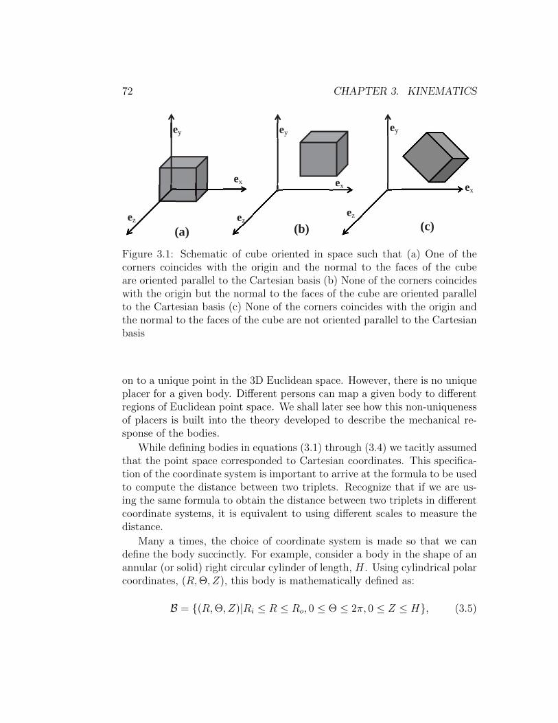
72 CHAPTER 3. KINEMATICS
ex ex
ey
ez
ex x
ey
ez
ex ex
ey
ez
(a) (b) (c)
Figure 3.1: Schematic of cube oriented in space such that (a) One of thecorners coincides with the origin and the normal to the faces of the cubeare oriented parallel to the Cartesian basis (b) None of the corners coincideswith the origin but the normal to the faces of the cube are oriented parallelto the Cartesian basis (c) None of the corners coincides with the origin andthe normal to the faces of the cube are not oriented parallel to the Cartesianbasis
on to a unique point in the 3D Euclidean space. However, there is no uniqueplacer for a given body. Different persons can map a given body to differentregions of Euclidean point space. We shall later see how this non-uniquenessof placers is built into the theory developed to describe the mechanical re-sponse of the bodies.
While defining bodies in equations (3.1) through (3.4) we tacitly assumedthat the point space corresponded to Cartesian coordinates. This specifica-tion of the coordinate system is important to arrive at the formula to be usedto compute the distance between two triplets. Recognize that if we are us-ing the same formula to obtain the distance between two triplets in differentcoordinate systems, it is equivalent to using different scales to measure thedistance.
Many a times, the choice of coordinate system is made so that we candefine the body succinctly. For example, consider a body in the shape of anannular (or solid) right circular cylinder of length, H. Using cylindrical polarcoordinates, (R,Θ, Z), this body is mathematically defined as:
B = (R,Θ, Z)|Ri ≤ R ≤ Ro, 0 ≤ Θ ≤ 2π, 0 ≤ Z ≤ H, (3.5)
3.2. BODY 73
where Ri and Ro are some positive constants, with Ri = 0 for a solid cylinder.Try defining this body using Cartesian coordinates.
Experience has shown that it is easier to do computations if we use vectorspace instead of point space. Naively, while in vector spaces we speak ofposition vectors of a point, in point space we speak about the coordinatesof a point. Next, we would like to establish this relationship between themathematical ideas of the vector space and point space. To do this, for eachordered pair of points (a, b) in the Euclidean point space E there corresponds
a unique vector in the Euclidean vector space, V, denoted by ~ab, with theproperties
(i) ~ba = −~ab, ∀ a, b ∈ E .
(ii) ~ab = ~ac + ~cb, ∀ a, b, c ∈ E .
(iii) Choosing arbitrarily a point o from E , and a Cartesian coordinate basisto span the vector space, V, there corresponds to each vector a ∈ V aunique point a ∈ E such that a = ~oa, the point o is called the originand a the position of a relative to o.
In other words, property (iii) states that the components of any vector a(a1, a2, a3) relative to a chosen Cartesian coordinate basis correspond to thecoordinates of some point a in E . The fact that this holds only for Carte-sian coordinate system cannot be overemphasized. To see this, recall that incylindrical polar coordinate system even though a triplet (R,Θ, Z) charac-terizes a point in E , position vectors have components of the form (R, 0, Z)only. That is the components of the position vector of a point is not sameas the coordinates of the point.
The notions of distance and angle in E are derived from the scalar producton the supporting vector space V: the distance between the arbitrary pointsa and b is defined by |~ab| and the angle, α subtended by a and b at a thirdarbitrary point c by
α = cos−1
(~ca · ~cb|~ca||~cb|
), (0 ≤ φ ≤ π). (3.6)
Thus, the choice of scale corresponds to the different expressions for thescalar product.
Considering the physical body to be made up of material particles, de-noted by P , we have seen how it can be mapped to the 3D Euclidean point

74 CHAPTER 3. KINEMATICS
space and hence to the 3D Euclidean vector space. Thus, the region occupiedby this body in the 3D Euclidean vector space is called as the configurationof the body and is denoted by B. Then, the placing function κ: B → B andits inverse κ−1: B → B are defined as:
X = κ(P ), P = κ−1(X). (3.7)
Recognize that the inverse exist because the mappings are one to one bydefinition. Henceforth, by placer we mean placing the body in the Euclideanvector space not the point space.
Next, let us understand what time is. Time concerns with the orderingof events. That is, it tells us whether an event occurred before or after aparticular event. We shall assume that we cannot count the number of events.Hence, we map the events to the points on a real line. This assumption thatthe number of events is countless, is required so that we can take derivativeswith respect to time. The part of the real line that is used to map a set ofevents is the prerogative of the person who establishes this correspondencewhich is similar to the mapping of the body on to the 3D Euclidean pointspace. The motion of a body is considered to be an event in mechanics.When a body moves, its configuration changes, that is the region occupiedby the body in the 3D Euclidean vector space changes.
Let t be a real variable denoting time such that t ∈ I ⊆ R, set of reals.If we could associate a configuration, Bt for the body B for each instant oftime in the interval of interest then the family of configurations Bt : t ∈ Iis called motion of B. Hence, we can define functions φ: B × I → Bt andφ−1: Bt × I → B such that
x = φ(P, t), P = φ−1(x, t). (3.8)
In a motion of B a typical particle, P occupies a succession of points whichtogether form a curve in E . This curve is called the path of P and is given ina parametric manner by equation (3.8a). The velocity and acceleration of Pare defined as rate of change of position and velocity with time, respectively,as P traverses its path.
While the definition of motion by (3.8a) is satisfactory, it would be usefulif it were to be a function of the vectors instead of points. To achieve this wemake use of the equation (3.7b). That is we choose a certain configurationof the body and identify the particles by the position vector of the point itoccupies in this configuration, then
x = φ(κ−1(X), t) = χκ(X, t). (3.9)
3.3. DEFORMATION GRADIENT 75
χκ is called the motion field and the subscript κ denotes that it depends onthe configuration which is used to identify the particles. The configuration inwhich the particles are identified is called the reference configuration and isdenoted by Br. This definition does not require the reference configurationto be a configuration actually occupied by the body during its motion. If thereference configuration were to be a configuration actually occupied by thebody during its motion at some time to, then (3.9) could be obtained from(3.8) as
x = φ(φ−1(X, to), t) = χto(X, t). (3.10)
We call χκ (or χto) the deformation field when it is independent of time orits dependence on time is irrelevant.
Now, we would like to make a few remarks. The definition of a bodyand motion is independent of whether we are concerned with rigid body ordeformable body. However, certain structures or details impounded on thebody depends on this choice. Till now, we have been talking about thebody being a set of particles but to be precise we should have said materialparticles. This detail is important within the context of deformable bodies,as we shall see later. It should also be remembered that the distinction thata given particle is steel or wood is made right in the beginning. Thus, withinthe realms of classical mechanics we cannot model chemically reacting bodywhere material particles of a particular type gets transformed into another.Because the body is considered to be a fixed set of material particles, theycannot die or be born or get transformed.
As we shall see later, an important kinematical quantity in the studyof deformable bodies is the gradient of motion. For us to be able to findthe gradient of motion, we require the motion field, (3.9) to be continuouson B and there should exist countless material particles of the same type(material) in spheres of radius, r for any value of r less than δo where δo issome constant. It is for this purpose, in the study of deformable bodies werequire the body to be a continuum.
3.3 Deformation Gradient
The gradient of motion is generally called the deformation gradient and isdenoted by F. Thus
F =∂x
∂X= O(x). (3.11)

76 CHAPTER 3. KINEMATICS
Since, χ is a function of both X and t we have used a partial derivative inthe definition of the deformation gradient. Also, we haven’t defined it asGrad(x) because for the Grad operator, as defined in chapter 2, the rangeof the function for which gradient is sought is any vector; not just positionvectors. The difference becomes evident in curvilinear coordinate systemslike the cylindrical polar coordinates.
Let Ei be the three Cartesian basis vectors in the reference configu-ration and ei the basis vectors in the current configuration. Then, thedeformation gradient is written as
F = Fijei ⊗ Ej. (3.12)
In general, the basis vectors ei and Ej need not be the same. Since thedeformation gradient depends on two sets of basis vectors, it is called a two-point tensor. It is pertinent here to point out that the grad operator asdefined in chapter 2 (2.207), is not a two-point tensor either. The matrixcomponents of the deformation gradient in Cartesian coordinate system is
(F)ij =
∂x∂X
∂x∂Y
∂x∂Z
∂y∂X
∂y∂Y
∂y∂Z
∂z∂X
∂z∂Y
∂z∂Z
, (3.13)
where (X, Y, Z) and (x, y, z) are the Cartesian coordinates of a typical mate-rial particle, P in the reference and current configuration respectively. Simi-larly, the matrix components of the deformation gradient in cylindrical polarcoordinate system is:
(F)ij =
∂r∂R
1R∂r∂Θ
∂r∂Z
r ∂θ∂R
rR∂θ∂Θ
r ∂θ∂Z
∂z∂R
1R∂z∂Θ
∂z∂Z
, (3.14)
where (R,Θ, Z) and (r, θ, z) are the cylindrical polar coordinates of a typicalmaterial particle, P in the reference and current configuration respectively.Substituting
X = R cos(Θ), Y = R sin(Θ), Z = Z,
x = r cos(θ), y = r sin(θ), z = z, (3.15)

3.4. LAGRANGIAN AND EULERIAN DESCRIPTION 77
in (3.13) we obtain
(F)xX(F)xY(F)xZ(F)yX(F)yY(F)yZ(F)zX(F)zY(F)zZ
=
∂r∂X
cos(θ)− r sin(θ) ∂θ∂X
∂r∂Y
cos(θ)− r sin(θ) ∂θ∂Y
∂r∂Z
cos(θ)− r sin(θ) ∂θ∂Z
∂r∂X
sin(θ) + r cos(θ) ∂θ∂X
∂r∂Y
sin(θ) + r cos(θ) ∂θ∂Y
∂r∂Z
sin(θ) + r cos(θ) ∂θ∂Z
∂z∂X∂z∂Y∂z∂Z
(3.16)
where
∂(·)∂X
= cos(Θ)∂(·)∂R− sin(Θ)
R
∂(·)∂Θ
, (3.17)
∂(·)∂Y
= sin(Θ)∂(·)∂R
+cos(Θ)
R
∂(·)∂Θ
, (3.18)
∂(·)∂Z
=∂(·)∂Z
, (3.19)
from which we obtain (3.14) recognizing that
ER = cos(Θ)E1 + sin(Θ)E2, er = cos(θ)e1 + sin(θ)e2,EΘ = − sin(Θ)E1 + cos(Θ)E2, eθ = − sin(θ)e1 + cos(θ)e2,EZ = E3, ez = e3,
where ER,EΘ,EZ and er, eθ, ez are the cylindrical polar coordinate basisvectors obtained from (2.242) using (3.15). Comparing equations (3.14) with(2.259) we see the difference between the Grad operator and O operator.
3.4 Lagrangian and Eulerian description
In the development of the basic principles of continuum mechanics, a body Bis endowed with various physical properties which are represented by scalaror tensor fields, defined either on a reference configuration, Br or on thecurrent configuration Bt. In the former case, the independent variables arethe position vectors of the particles in the reference configuration, X andtime, t. This characterization of the field with X and t as independent

78 CHAPTER 3. KINEMATICS
variables is called Lagrangian (or material) description. In the latter case,the independent variables are the position vectors of the particles in thecurrent configuration, x and time, t. The characterization of the field withx and t as independent variables is called Eulerian (or spatial) description.Thus, density, displacement and stress are examples of scalar, vector andsecond order tensor fields respectively and can be represented as
ρ = ρ(X, t) = ρ(x, t), (3.20)
u = u(X, t) = u(x, t), (3.21)
σ = σ(X, t) = σ(x, t), (3.22)
where the second equality is obtained by using the relation X = χ−1κ (x, t),
which is possible because the function χκ in (3.9) is one to one. Here functionswith a hat denote that the independent variables are X and t, while functionswith a tilde denote that the independent variables are x and t.
To understand the difference between the Lagrangian description andEulerian description, consider the flow of water through a pipe from a largetank. Now, if we seed the tank with micro-spheres and determine the velocityof these spheres as a function of time and their initial position in the tankthen we get the Lagrangian description for the velocity. On the other hand,if we choose a point in the pipe and determine the velocity of the particlescrossing that point as a function of time then we get the Eulerian descriptionof velocity. While in fluid mechanics we use the Eulerian description, in solidmechanics we use Lagrangian description, mostly.
Next, we define what is called as the material time derivative or La-grangian time derivative or total time derivative and spatial time derivativeor Eulerian time derivative. It could be inferred from the above that variousvariables of interest are functions of time, t and either X or x. Hence, whenwe differentiate these variables with respect to time, we can hold either X aconstant or x a constant. If we hold X a constant while differentiating withtime, we call such a derivative total time derivative and denote it by D(·)
Dt.
On the other hand if we hold x a constant, we call it spatial time derivativeand denote it by d(·)
dt. Thus, for the scalar field defined by, say (3.20) we have
Dρ
Dt=
∂ρ
∂t=∂ρ
∂t+ grad(ρ) · v, (3.23)
dρ
dt=
∂ρ
∂t=∂ρ
∂t+Grad(ρ) · dX
dt, (3.24)
3.5. DISPLACEMENT, VELOCITY AND ACCELERATION 79
where grad(·) stands for the gradient with respect to x, Grad(·) stands for thegradient with respect to X and v = Dx
Dt. The above equations are obtained
by using the chain rule. Similarly, for a vector field defined by (3.21) we have
Du
Dt=
∂u
∂t=∂u
∂t+ grad(u)v, (3.25)
du
dt=
∂u
∂t=∂u
∂t+Grad(u)
dX
dt. (3.26)
Recognize that DXDt
= o and dxdt
= o.Finally, a note on the notation. If the starting letter is capitalized for any
of the operators introduced in chapter 2 then it means that the derivative iswith respect to the material coordinates, i.e. X otherwise, the derivative iswith respect to the spatial coordinates, i.e. x. In the above, we have alreadyused this convention for the gradient operator.
3.5 Displacement, velocity and acceleration
The vector field, u, defined as
u = x−X, (3.27)
represents the displacement field, that is the displacement of the materialparticles initially at X or currently at x depending on whether Lagrangianor Eulerian description is used. Thus,
u(X, t) = χκ(X, t)−X, (3.28)
u(x, t) = x− χ−1κ (x, t). (3.29)
Figure 3.2 schematically shows the displacement vector. As shown in thefigure, displacement vector is a straight line segment joining the locationof a material particle in the current and reference configuration. While,in the schematic we have used the same coordinate system to describe allthe three directed line segments namely, the position vector of a particlein the reference configuration, current configuration and the displacementvector; this is not necessary. In fact, if one uses cylindrical polar coordinatebasis, the position vector of the material particle in the current and referenceconfiguration, in general would be different.
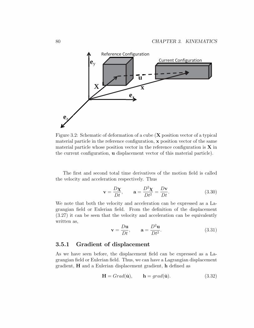
80 CHAPTER 3. KINEMATICS
ex ex
ey
ez
X x u
Current Configuration Reference Configuration
Figure 3.2: Schematic of deformation of a cube (X position vector of a typicalmaterial particle in the reference configuration, x position vector of the samematerial particle whose position vector in the reference configuration is X inthe current configuration, u displacement vector of this material particle).
The first and second total time derivatives of the motion field is calledthe velocity and acceleration respectively. Thus
v =Dχ
Dt, a =
D2χ
Dt2=Dv
Dt. (3.30)
We note that both the velocity and acceleration can be expressed as a La-grangian field or Eulerian field. From the definition of the displacement(3.27) it can be seen that the velocity and acceleration can be equivalentlywritten as,
v =Du
Dt, a =
D2u
Dt2. (3.31)
3.5.1 Gradient of displacement
As we have seen before, the displacement field can be expressed as a La-grangian field or Eulerian field. Thus, we can have a Lagrangian displacementgradient, H and a Eulerian displacement gradient, h defined as
H = Grad(u), h = grad(u). (3.32)

3.5. DISPLACEMENT, VELOCITY AND ACCELERATION 81
Recognize that these gradients are not the same. To see this, we computethe displacement gradient in terms of the deformation gradient as
H = Grad(u) =∂x
∂X− ∂X
∂X= F− 1, (3.33)
h = grad(u) =∂x
∂x− ∂X
∂x= 1− F−1, (3.34)
3.5.2 Example
A certain motion of a continuum body in the material description is given inthe form:
x1 = X1 − exp(−t)X2, x2 = exp(−t)X1 +X2, x3 = X3, (3.35)
for t > 0. Find the displacement, velocity and acceleration componentsin terms of the material and spatial coordinates and time. Also find thedeformation and displacement. Assume that the same Cartesian coordinatebasis and origin is used to describe the body both in the current and thereference configuration.
It follows from (3.27) that
u = − exp(−t)X2E1 + exp(−t)X1E2. (3.36)
Similarly, from (3.30) we obtain
v = exp(−t)X2E1 − exp(−t)X1E2, (3.37)
a = − exp(−t)X2E1 + exp(−t)X1E2, . (3.38)
Inverting the motion field (3.35) we obtain
X1 =[x1 + exp(−t)x2]
[1 + exp(−2t)], X2 =
[x2 − exp(−t)x1]
[1 + exp(−2t)], X3 = x3. (3.39)
Substituting (3.39) in (3.36), (3.37) and (3.38) we obtain the Eulerianform of the displacement, velocity and acceleration fields as
u = − [x2 − exp(−t)x1]
[1 + exp(−2t)]exp(−t)E1 +
[x1 + exp(−t)x2]
[1 + exp(−2t)]exp(−t)E2,
v =[x2 − exp(−t)x1]
[1 + exp(−2t)]exp(−t)E1 −
[x1 + exp(−t)x2]
[1 + exp(−2t)]exp(−t)E2,
a = − [x2 − exp(−t)x1]
[1 + exp(−2t)]exp(−t)E1 +
[x1 + exp(−t)x2]
[1 + exp(−2t)]exp(−t)E2.
82 CHAPTER 3. KINEMATICS
Here we have made use of the fact that the same Cartesian basis vectors areused to define both the current and the reference configuration.
Next, we compute the deformation gradient to be
F =
1 − exp(−t) 0exp(−t) 1 0
0 0 1
, (3.40)
and the Lagrangian and Eulerian displacement gradient as
H =
0 − exp(−t) 0exp(−t) 0 0
0 0 0
, (3.41)
h =
exp(−2t)
[1+exp(−2t)]− exp(−t)
[1+exp(−2t)]0
exp(−t)[1+exp(−2t)]
exp(−2t)[1+exp(−2t)]
0
0 0 0
, (3.42)
Notice that at t = 0, F 6= 1, but F tends to 1 as time, t tends to∞. This justindicates that the configuration chosen as reference is not the one at time t= 0, but at some other time and this is permissible.
3.6 Transformation of curves, surfaces and
volume
Before rigorously deriving the general expressions for transformation of curves,surfaces and volumes, let us obtain these expressions after various simplifyingassumptions.
Let us assume the following:
1. The same Cartesian coordinate basis and origin is used to describe thebody in both its reference and current configuration.
2. The body is subjected to displacement u and the Lagrangian descrip-tion of the displacement field is known and is sufficiently smooth forthe required derivatives to exist. That is
u = ux(X, Y, Z)ex + uy(X, Y, Z)ey + +uz(X, Y, Z)ez, (3.43)

3.6. TRANSFORMATION OF CURVES, SURFACES AND VOLUME 83
ey
ex exxxxxxxxxxxxxxxxxxxxxxxxxxxxx
ez
Xo xo
x1 X1
u(Xo+ΔX, Yo, Zo)
x1u(Xo, Yo, Zo)
Reference Configuration
Current Configuration
Figure 3.3: Schematic of the deformation of a line oriented along ex of length∆X.
where ux(X, Y, Z), uy(X, Y, Z) and uz(X, Y, Z) are some known func-tions of the X, Y and Z the coordinates of the material particles inthe reference configuration.
3. It is assumed that the components of the displacement can be approx-imated as
ux(Xo + ∆X, Yo + ∆Y, Zo + ∆Z) ≈ ux(Xo, Yo, Zo)
+∂ux∂X
∣∣∣∣(Xo,Yo,Zo)
∆X +∂ux∂Y
∣∣∣∣(Xo,Yo,Zo)
∆Y +∂ux∂Z
∣∣∣∣(Xo,Yo,Zo)
∆Z,
uy(Xo + ∆X, Yo + ∆Y, Zo + ∆Z) ≈ uy(Xo, Yo, Zo)
+∂uy∂X
∣∣∣∣(Xo,Yo,Zo)
∆X +∂uy∂Y
∣∣∣∣(Xo,Yo,Zo)
∆Y +∂uy∂Z
∣∣∣∣(Xo,Yo,Zo)
∆Z,
uz(Xo + ∆X, Yo + ∆Y, Zo + ∆Z) ≈ uz(Xo, Yo, Zo)
+∂uz∂X
∣∣∣∣(Xo,Yo,Zo)
∆X +∂uz∂Y
∣∣∣∣(Xo,Yo,Zo)
∆Y +∂uz∂Z
∣∣∣∣(Xo,Yo,Zo)
∆Z,
(3.44)

84 CHAPTER 3. KINEMATICS
where the displacement of the material particle occupying the point Xo
is u(Xo, Yo, Zo) and that displacement of the material particle that isoccupying, X1 is u(Xo + ∆X, Yo + ∆Y, Zo + ∆Z). Here it is pertinentto point out that the above is a truncated Taylor’s series. Since, weare interested in arbitrarily small values of ∆X, ∆Y , ∆Z, we havetruncated the Taylor’s series after the first term. However, this is nota valid approximation for many functions. For example, functions ofthe form aX3/2, where a is a constant defined over the domain, say0.01 ≤ X ≤ 0.1 the value of the derivatives greater then second orderwould be more than the first order derivative. Hence, the expressionderived based on this assumption, though intuitive has its limitations.
First, we are interested in finding how the length of the straight line oflength ∆X oriented along the ex direction in the reference configuration of thebody, as shown in the figure 3.3 has changed. With the above assumptions,the deformed length of the straight line of length ∆X oriented along the exdirection in the reference configuration is given by,
‖x1 − xo‖ = ‖X1 −Xo + u(X1)− u(Xo)‖
= ∆X
√[1 +
∂ux∂X
]2
+
[∂uy∂X
]2
+
[∂uz∂X
]2
, (3.45)
where X1 = Xo + ∆Xex, xo denotes the current position vector of the ma-terial particle whose position in the reference configuration is Xo, x1 denotesthe current position vector of the material particle whose position in the ref-erence configuration is X1 and use is made of equation (3.44). Now, if themagnitude of the components of the gradient of the displacement are small(say of the magnitude of 10−3), then equation (3.45) could be approximatelycalculated as,
‖x1 − xo‖ = ∆X
[1 +
∂ux∂X
]. (3.46)
Hence, the stretch ratio defined as the ratio of the current length to theundeformed length for a line element oriented along the ex direction is,
Λ(ex) =‖x1 − xo‖‖X1 −Xo‖
=
√[1 +
∂ux∂X
]2
+
[∂uy∂X
]2
+
[∂uz∂X
]2
≈[1 +
∂ux∂X
]. (3.47)

3.6. TRANSFORMATION OF CURVES, SURFACES AND VOLUME 85
ey
ex exxxxxxxxxxxxxxxxxxxxxxxxxxxx
ez
Xo xo
x1
X1
X2
x2
Reference Configuration Current Configuration
Figure 3.4: Schematic of the deformation of a face of the cube.
which can be approximately computed as,
Λ(ex) ≈[1 +
∂ux∂X
]. (3.48)
when the components of the displacement gradient are small. Following asimilar procedure, one can determine how the length of line elements orientedalong any direction changes. We shall derive a general expression for the samelater in section 3.6.1.
Next we are interested in finding how the area of a face of a small cuboidchanges due to deformation. Let us assume that the face of the cuboid whosenormal coincides with the ez basis is of interest and the sides of this face ofthe cuboid are of length ∆X along the ex direction and ∆Y along the eydirection. Thus, as shown in figure 3.4, Xo (= Xoex + Yoey + Zoez), X1 (=(Xo+∆X)ex+Yoey+Zoez) and X2 (= Xoex+(Yo+∆Y )ey+Zoez) denote theposition vector of the three corners of the face of the cuboid whose normalis ez in the reference configuration and xo, x1 and x2 denote the position ofthe same three corners of the face of the cuboid in the current configuration.For the same three assumptions listed above, the deformed area of this face

86 CHAPTER 3. KINEMATICS
of the cuboid is given by,
a = ‖(x1 − xo) ∧ (x2 − xo)‖= ‖(X1 −Xo + u(X1)− u(Xo)) ∧ (X2 −Xo + u(X2)− u(Xo))‖
= (∆X)(∆Y )
∣∣∣∣[∂uy∂X
∂uz∂Y− ∂uz∂X
(1 +
∂uy∂Y
)]ex
+
[∂uz∂X
∂ux∂Y−(
1 +∂ux∂X
)∂uz∂Y
]ey
+
[(1 +
∂ux∂X
)(1 +
∂uy∂Y
)− ∂uy∂X
∂ux∂Y
]ez
∣∣∣∣ , (3.49)
and the orientation of the normal to this deformed face is computed as,
n =(x1 − xo) ∧ (x2 − xo)
‖(x1 − xo) ∧ (x2 − xo)‖
=(X1 −Xo + u(X1)− u(Xo)) ∧ (X2 −Xo + u(X2)− u(Xo))
‖(X1 −Xo + u(X1)− u(Xo)) ∧ (X2 −Xo + u(X2)− u(Xo))‖. (3.50)
Recollect that in chapter 2 we mentioned that the cross product of two vectorscharacterizes the area of the parallelogram spanned by them. We have madeuse of this to obtain the above expressions.
Finally, we find the volume of the deformed cuboid. Again recollectingfrom chapter 2, the box product of three vectors yields the volume of theparallelepiped spanned by them, the deformed volume of the cuboid is givenby,
v = [x1 − xo,x2 − xo,x3 − xo]
= (∆X)(∆Y )(∆Z)
[(1 +
∂uz∂Z
)(1 +
∂uy∂Y
)− ∂uy∂Z
∂uz∂Y
](1 +
∂ux∂X
)+
[∂uz∂Y
∂ux∂Z−(
1 +∂uz∂Z
)∂ux∂Y
]∂uy∂X
+
[∂ux∂Y
∂uy∂Z−(
1 +∂uy∂Y
)∂ux∂Z
]∂uz∂X
, (3.51)
where xo, x1, x2 and x3 are the position vectors of the material particlesin the current configuration corresponding to whose position vector in thereference configuration are Xo (= Xoex+Yoey+Zoez), X1 (= (Xo+∆X)ex+

3.6. TRANSFORMATION OF CURVES, SURFACES AND VOLUME 87
Yoey +Zoez), X2 (= Xoex + (Yo + ∆Y )ey +Zoez) and X3 (= Xoex + Yoey +(Zo + ∆Z)ez) respectively.
When the magnitude of the components of the displacement gradientare small, then the deformed volume of the cuboid could be computed fromequation (3.51) as,
v ≈ (∆X)(∆Y )(∆Z)
[1 +
∂ux∂X
+∂uy∂Y
+∂uz∂Z
], (3.52)
by neglecting the quadratic and cubic terms in equation (3.51).
3.6.1 Transformation of curves
We know the position vector of any particle belonging to the body at variousinstances of time, t. But now we are interested in finding how a set of con-tiguous points forming a curve changes its shape. That is, we are interestedin finding how a circle inscribed in the reference configuration changes itsshape, say into an ellipse, in the current configuration. As we have requiredthe deformation field to be one to one, closed curves like circle, ellipse, willremain as closed curves and open curves like straight line, parabola remainsopen. The position vectors of the particles that occupy a curve can be de-scribed using a single variable, say ξ. For example, a circle of radius R inthe plane whose normal coincides with ez, as shown in figure 3.5a wouldbe described as (R cos(ξ), R sin(ξ), Zo), where R and Zo are constants and 0≤ ξ ≤ 2π.
Consider a material curve (or a curve in the reference configuration), X= Γ(ξ) ⊂ Br, where ξ denotes a parametrization. The material curve byvirtue of it being defined in the reference configuration is not a function oftime. During a certain motion, the material curve deforms into another curvecalled the spatial curve, x = γ(ξ, t) ⊂Bt, (see figure 3.5b). The spatial curveat a fixed time t is then defined by the parametric equation
x = γ(ξ, t) = χ(Γ(ξ), t). (3.53)
We denote the tangent vector to the material curve as ∆X and the tangentvector to the spatial curve as ∆x and are defined by
∆X =dΓ
dξ∆ξ, ∆x =
∂γ
∂ξ∆ξ (3.54)
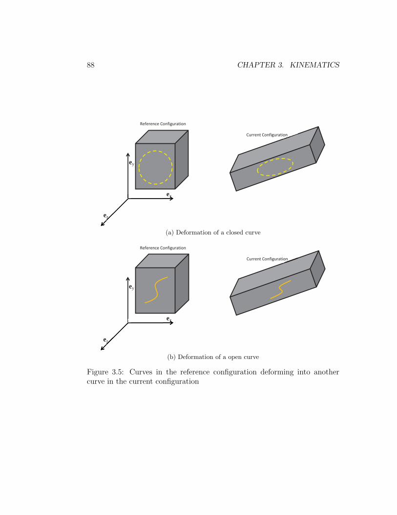
88 CHAPTER 3. KINEMATICS
ey
ex exxxxxxxxxxxxxxxxxxxxxxxxxxxxx
ez
Reference Configuration
Current Configuration
(a) Deformation of a closed curve
ey
ex exxxxxxxxxxxxxxxxxxxxxxxxxxx
ez
Reference Configuration
Current Configuration
(b) Deformation of a open curve
Figure 3.5: Curves in the reference configuration deforming into anothercurve in the current configuration

3.6. TRANSFORMATION OF CURVES, SURFACES AND VOLUME 89
By using (3.53) and the chain rule we find that
∂γ
∂ξ=∂χ
∂X
dX
dξ=∂χ
∂X
dΓ
dξ. (3.55)
Hence, from equation (3.54) and the definition of the deformation gradient,(3.11) we find that
∆x = F∆X. (3.56)
Expression (3.56) clearly defines a linear transformation which generatesa vector ∆x by the action of the second-order tensor F on the vector ∆X. Insummary: material tangent vectors map into spatial tangent vectors via thedeformation gradient. This is the physical significance of the deformationgradient.
In the literature, the tangent vectors ∆x and ∆X, in the current andreference configuration are often referred to as the spatial line element andthe material line element, respectively. This is correct only when the curvein the reference and current configuration is a straight line.
Next, we introduce the concept of stretch ratio which is defined as theratio between the current length to its original length. When we say originallength, we mean undeformed length, that is the length of the fiber when it isnot subjected to any force. It should be pointed out at the outset that manya times the undeformed length would not be available and in these cases itis approximated as the length in the reference configuration.
In general, the stretch ratio depends on the location and orientation of thematerial fiber for which it is computed. Thus, we can fix the orientation of thematerial fiber in the reference configuration or in the current configuration.Corresponding to the configuration in which the orientation of the fiber isfixed we have two stretch measures. Recognize that we can fix the orientationof the fibers in only one configuration because its orientation in others isdetermined by the motion.
First, we consider deformations in which any straight line segments inthe reference configuration gets mapped on to a straight line segment in thecurrent configuration. Such a deformation field which maps straight line seg-ments in the reference configuration to straight line segments in the currentconfiguration is called homogeneous deformation. We shall in section 3.10,illustrate that when the deformation is homogeneous, the Cartesian compo-nents of the deformation gradient would be a constant. As a consequenceof assuming the curve to be a straight line, the tangent and secant to the

90 CHAPTER 3. KINEMATICS
curve is the same. Hence, saying that we are considering a material fiber3 oflength ∆L initially oriented along A, (where A is a unit vector) and locatedat P, is same as saying that we are studying the influence of the deformationon the tangent vector, ∆LA at P. Due to some motion of the body, thematerial particle that occupied the point P will occupy the point p ∈ Bt
and the tangent vector ∆LA is going to be mapped on to a tangent vectorwith length, say ∆l and orientation a. From (3.56) we have
∆la = ∆LFA. (3.57)
Dotting the above equation with ∆la, we get
(∆l)2 = (∆L)2FA · FA = (∆L)2FtFA ·A, (3.58)
where we have used the fact that a is a unit vector, the relation (3.57) andthe definition of transpose. Defining the right Cauchy-Green deformationtensor, C as
C = FtF, (3.59)
and using equation (3.58) we obtain
ΛA =∆l
∆L=√
CA ·A, (3.60)
where ΛA represents the stretch ratio of a line segment initially orientedalong A. The stretch ratio, ΛA is the one that could be directly determinedin an experiment. However, there is no reason why we should restrict ourstudies to line segments which are initially oriented along a given direction.We can also study about material fibers that are finally oriented along agiven direction. Towards this, we invert equation (3.57) to get
∆LA = ∆lF−1a. (3.61)
Dotting the above equation with ∆LA, we get
(∆L)2 = (∆l)2F−1a · F−1a = (∆l)2F−tF−1a · a, (3.62)
using arguments similar to that used to get (3.58) from (3.57). Defining theleft Cauchy-Green deformation tensor or the Finger deformation tensor, Bas
B = FFt, (3.63)
3A material fiber is also sometimes called as infinitesimal line elements.

3.6. TRANSFORMATION OF CURVES, SURFACES AND VOLUME 91
and using equation (3.62) we obtain
Λa =∆l
∆L=
1√B−1a · a
, (3.64)
where Λa represents the stretch ratio of a fiber finally oriented along a.Next, we would like to compute the final angle between two two straight
line segments initially oriented along A1 and A2. Recognizing that the anglebetween two straight line segments, α is computed using the expression:
α = cos−1
(A1 ·A2
|A1||A2|
). (3.65)
Using (3.65) and similar arguments as that used to obtain the stretch ratio,it can be shown that the final angle, αf between the straight line segmentsinitially oriented along A1 and A2 is given by
αf = cos−1
(CA1 ·A2√
CA1 ·A1
√CA2 ·A2
). (3.66)
Just, as in the case of stretch ratio, we can also study the initial angle, αibetween straight line segments that are finally oriented along a1 and a2. Forthis case, following the same steps outlined above we compute
αi = cos−1
(B−1a1 · a2√
B−1a1 · a1
√B−1a2 · a2
). (3.67)
We like to record that as in the case of stretch ratio, αi and αf depends onthe orientation of the line segments.
Next, let us see what happens when the deformation is inhomogeneous.For inhomogeneous deformation, the Cartesian components of the deforma-tion gradient would vary spatially and the straight line segment in the refer-ence configuration would have become a curve in the current configuration.Hence, distinction between the tangent and the secant has to be made. Now,the deformed length of the curve, ∆l corresponding to that of a straight lineof length ∆L oriented along A is obtained from equation (3.56) as,
∆l =
∫ 1
0
√(dx
dξ
)2
+
(dy
dξ
)2
+
(dz
dξ
)2
dξ
=
∫ 1
0
√√√√CA ·A
[(dX
dξ
)2
+
(dY
dξ
)2
+
(dZ
dξ
)2]dξ, (3.68)

92 CHAPTER 3. KINEMATICS
ey
ex exx
ez
(Xo, Yo, Zo)
(Xo, Yo+ΔL, Zo)
Reference Configuration
(a) Straight line oriented along Ey
at (Xo, Yo, Zo).
ey
ex exx
ez
(Xo, Yo, Zo)
y(Xo+0.6ΔL,Yo+0.8ΔL, Zo)
Reference Configuration
(b) Straight line oriented along(3Ex + 4Ey)/5 at (Xo, Yo, Zo).
Figure 3.6: Schematic of straight lines in a body
where A is a constant vector, C = C(X(ξ), Y (ξ), Z(ξ)), (X(ξ), Y (ξ), Z(ξ))denotes the coordinates of the material points that constitutes the straightline and ξ varies between 0 and 1 to parameterize the straight line. Thus,for a line oriented along say Ey direction of length ∆L, starting from a point(Xo, Yo, Zo), (see figure 3.6a) X(ξ) = Xo, Y (ξ) = Yo + ξ(∆L), Z(ξ) = Zo.For a line oriented along say (3Ex + 4EY )/5 of length ∆L, starting from(Xo, Yo, Zo), (see figure 3.6b) X(ξ) = Xo+3ξ(∆L)/5, Y (ξ) = Yo+4ξ(∆L)/5,Z(ξ) = Zo. In fact, if one relaxes the assumption that A is a constant inequation (3.68) then the straight line in the reference configuration could bea curve and the deformed length could still be calculated from (3.68).
Hence, the stretch ratio for the case of inhomogeneous deformation is,
ΛA =∆l
∆L=
∫ ξ1ξo
√CA ·A
√(dXdξ
)2
+(dYdξ
)2
+(dZdξ
)2
dξ
∫ ξ1ξo
√(dXdξ
)2
+(dYdξ
)2
+(dZdξ
)2
dξ
. (3.69)

3.6. TRANSFORMATION OF CURVES, SURFACES AND VOLUME 93
3.6.2 Transformation of areas
Having seen how points, curves, tangent vectors in the reference configura-tion gets mapped to points, curves and tangent vectors in the current con-figuration, we are now in a position to look at how surfaces get mapped. Ofinterest, is how a unit vector, N normal to an infinitesimal material surfaceelement ∆A map on to a unit vector n normal to the associated infinitesimalspatial surface element ∆a.
Let Sr denote the material surface in Br that is of interest. Then, anelement of area ∆A at a point P on Sr is defined through the vectors ∆Xand ∆Y, each tangent to Sr at P, as ∆AN = ∆X ∧∆Y where N is a unitvector normal to Sr at P. Due to some motion of the body, the materialsurface Sr gets mapped on to another material surface St in Bt, the materialparticle that occupied the point P on Sr gets mapped onto a point p onSt and the tangent vectors ∆X and ∆Y gets mapped on to another pair oftangent vectors at p denoted by ∆x and ∆y. Thus, we have
∆AN = ∆X ∧∆Y, ∆an = ∆x ∧∆y. (3.70)
Since, ∆X and ∆Y are tangent vectors we have ∆x = F∆X and ∆y =F∆Y. Therefore,
∆an = (F∆X) ∧ (F∆Y) = F∗(∆X ∧∆Y) = det(F)F−tN∆A, (3.71)
where we have made use of (2.88) and (2.90). Thus, the relation
∆an = det(F)F−tN∆A, (3.72)
called Nanson’s formula is an often used expression in continuum mechanics.Next, we are interested in computing the deformed area, a. For this case,
from Nanson’s formula we obtain,
(∆a)n · (∆a)n = det(F)F−tN(∆A) · det(F)F−tN(∆A), (3.73)
which simplifies to
a =
∫A
det(F)√
C−1N ·NdA. (3.74)
on using the equation (3.59) and the fact that n is a unit vector. Noticethat, once again the deformed area is determined by the right Cauchy-Greendeformation tensor.

94 CHAPTER 3. KINEMATICS
3.6.3 Transformation of volumes
Next, we seek to obtain the relation between elemental volumes in the ref-erence and current configuration. An element of volume ∆V at a inte-rior point P in reference configuration is given by the scalar triple product[∆X,∆Y,∆Z] where ∆X, ∆Y and ∆Z are vectors oriented along the sidesof an infinitesimal parallelepiped. Since, the point under consideration is in-terior, we can always find three material curves such that they pass throughthe point P and ∆X, ∆Y and ∆Z are its tangent vectors at P. Now say dueto some motion of the body, the material particle that occupied the pointP, now occupies the point p, then the curves under investigation would passthrough p and the tangent vectors of these curves at this point p would nowbe ∆x, ∆y, ∆z. Hence,
∆v = [∆x,∆y,∆z] = [F∆X,F∆Y,F∆Z] = det(F)[∆X,∆Y,∆Z]
= det(F)∆V, (3.75)
where we have used the definition of the determinant (2.77). Since, thecoordinate basis vectors for the reference and current configuration have thesame handedness, det(F) ≥ 0. Further since, we require the mapping of thebody from one configuration to the other be one to one, material particlesin a parallelepiped cannot be mapped on to a surface. Hence, det(F) 6= 0.Therefore det(F) > 0. Thus, for a vector field to be a deformation field,det(F) > 0.
3.7 Properties of the deformation tensors
Since det(F) > 0, using the polar decomposition theorem (2.116) the defor-mation gradient can be represented as:
F = RU = VR, (3.76)
where R is a proper orthogonal tensor, U and V are the right and left stretchtensors respectively. (These stretch tensors are called right and left becausethey are on the right and left of the orthogonal tensor, R.) These stretchtensors are unique, positive definite and symmetric.
Substituting (3.76) in (3.59) and (3.63) we obtain
C = U2 = RtV2R, B = V2 = RU2Rt. (3.77)

3.8. STRAIN TENSORS 95
Next, we record certain properties of the right and left Cauchy-Greendeformation tensors.
1. The right Cauchy-Green deformation tensor, C depends only on thecoordinate basis used in the reference configuration, i.e., C = CijEi⊗Ej
= FaiFajEi ⊗ Ej
2. The left Cauchy-Green deformation tensor depends only on the coor-dinate basis used in the current configuration, i.e., B = Bijei ⊗ ej =FiaFjaei ⊗ ej
3. It is easy to see that both the tensors C and B are symmetric andpositive definite.
4. Since the deformation tensors are symmetric, they have three real prin-cipal values and their principal directions are orthonormal.
5. Both these tensors have the same eigen or principal values but differ-ent eigen or principal directions. To see this, let Na be the principaldirection of the tensor U and εa its principal value that is
UNa = εaNa, (3.78)
thenCNa = U2Na = ε2
aNa. (3.79)
Now let na = RNa. Then
Bna = RU2RtRNa = ε2aRNa = ε2
ana. (3.80)
Thus, we have shown that ε2a is the principal value for both C and B
tensors and Na and RNa are their principal directions respectively.
3.8 Strain Tensors
Now, we shall look at the concept of strain. This is some quantity definedby us and hence there are various definitions of the same. Also, as we shallsee later, we can develop the constitutive relation independent of these def-initions. Experimental observations show that relative displacement of par-ticles alone gives raise to stress. A measure of this relative displacement is

96 CHAPTER 3. KINEMATICS
the stretch ratio. However, this measure has the drawback that when thebody is not deformed the stretch ratio is 1 (by virtue of the deformed lengthbeing same as the original length) and hence thought to be inconvenient toformulate constitutive relations. Consequently, another measure of relativedisplacement is sought which would be 0 when the body is not deformed andless than zero when compressed and greater than zero when stretched. Thismeasure is called as the strain, ε(A). There is no unique way of obtaining thestrain from the stretch ratio. The following functions satisfy the requirementof the strain:
ε(A) =Λm
(A) − 1
m, ε(A) = ln(Λ(A)), (3.81)
where m is some real number and ln stands for natural logarithm. Thus, ifm = 1 in (1.5a) then the resulting strain is called as the engineering strain,if m = −1, it is called as the true strain, if m = 2 it is Cauchy-Green strain.The second function wherein ε(A) = ln(λ(A)), is called as the Hencky strainor the logarithmic strain.
Let us start by looking at the case when m = 2 in equation (3.81), thatis the case,
εCG(A) =Λ2
(A) − 1
2. (3.82)
Substituting (3.60) in (3.82) we obtain
εCG(A) =1
2(CA ·A− 1) =
1
2(C− 1)A ·A = EA ·A, (3.83)
where, E = 0.5[C − 1], is called the Cauchy-Green strain tensor. Thus,Cauchy-Green strain tensor carries information about the strain in the mate-rial fibers initially oriented along a given direction. Substituting Lagrangiandisplacement gradient, defined in (3.33), for deformation gradient in the ex-pression for E, we obtain
E =1
2[H + Ht + HtH]. (3.84)
If tr(HHt) << 1, i.e., each of the components of H is close to zero4, then wecan compute E approximately as
E ≈ 1
2[H + Ht] = εL. (3.85)
4Realize that tr(HHt) = H211 + H2
12 + H213 + H2
21 + H222 + H2
23 + H231 + H2
32 + H233
3.8. STRAIN TENSORS 97
εL is called as the Lagrangian linearized strain and will be used extensivelywhile studying linearized elasticity.
Next, we examine the case when m = 1, in equation (3.81), that is thecase,
εLS(A) = Λ(A) − 1. (3.86)
Substituting (3.60) in (3.86) we obtain
εLS(A) =√
CA ·A− 1. (3.87)
Substituting Lagrangian displacement gradient, defined in (3.33), for defor-mation gradient in the expression for C and using the definition (3.85) forLagrangian linearized strain, equation (3.87) evaluates to
εLS(A) =√
1 + 2εLA ·A + (HtH)A ·A− 1, (3.88)
which when the components of the Lagrangian displacement gradient aresmall could be approximately computed as
εLS(A) =√
1 + 2εLA ·A− 1 ≈ εLA ·A, (3.89)
where we have approximately evaluated the square root using Taylor’s se-ries5. Thus, Lagrangian linearized strain carries the information on changesin length of material fibers initially oriented along a given direction when thechanges in length are small.
Instead of studying the strain in fibers oriented initially along a givendirection, one can also study strains in fibers finally oriented along a givendirection, a. Now, again the following functions satisfy the requirement ofthe strain:
ε(a) =Λm
(a) − 1
m, ε(a) = ln(Λ(a)), (3.90)
where m is some real number and ln stands for natural logarithm. We studythe case when m = −2 in equation (3.90), that is the case,
εAH(a) =1− Λ−2
(a)
2. (3.91)
Substituting (3.64) in (3.91) and rearranging we obtain
εAH(A) =1
2(1−B−1a · a) =
1
2(1−B−1)a · a = ea · a. (3.92)
5√
1 + 2x ≈ 1 + x, when x is small.

98 CHAPTER 3. KINEMATICS
where, e = 0.5[1 − B−1], is called the Almansi-Hamel strain tensor andcarries information about the strain in the material fibers finally orientedalong a given direction. Substituting Eulerian displacement gradient, definedin (3.34), for F−1 in the expression for e, we obtain
e =1
2[h + ht − hth]. (3.93)
If tr(hht) << 1, then we can compute e approximately as
e ≈ 1
2[h + ht] = εE. (3.94)
εE is called as the Eulerian linearized strain.The Lagrangian and Eulerian displacement gradients are related through
the equationH = h + hH, (3.95)
obtained from the requirement that FF−1 = 1 and substituting the expres-sions (3.33) and (3.34) for F and F−1 respectively. It immediately transpiresthat when each of the components of H and h are close to zero then H ≈h and hence both the Lagrangian and Eulerian linearized strain are numeri-cally the same. Hence, when the distinction is not important the subscript,
L or E would be dropped and the linearized strain denoted as εThere are other strain measures called the Hencky strain tensor in the
Lagrangian and Eulerian form defined as ln(U) and ln(V) respectively. Thisstrain tensor corresponds the case where the strain along a given direction isdefined as the natural logarithm of the corresponding stretch ratio. Henckystrain is also sometimes called as the logarithmic strain.
3.9 Normal and shear strain
From now on we shall in this course, study the response of bodies only forcases when the value of the components of both the Lagrangian and Euleriandisplacement gradient are small. As we have shown above, this means thatnot only does the changes in length be small but the rotations also needsto be small. Under these severe but practically reasonable assumptions, thestrain-displacement relation is
ε =1
2
[h + ht
], (3.96)

3.9. NORMAL AND SHEAR STRAIN 99
where we stop distinguishing between Lagrangian and Eulerian gradient, asthey would be approximately the same. Thus, the Cartesian components ofthe linearized strain are,
ε =
εxx εxy εxzεxy εyy εyzεxz εyz εzz
=
∂ux∂x
12
[∂ux∂y
+ ∂uy∂x
]12
[∂ux∂z
+ ∂uz∂x
]12
[∂ux∂y
+ ∂uy∂x
]∂uy∂y
12
[∂uy∂z
+ ∂uz∂y
]12
[∂ux∂z
+ ∂uz∂x
]12
[∂uy∂z
+ ∂uz∂y
]∂uz∂z
(3.97)
where if the displacement field is given a Lagrangian description we woulduse a Lagrangian gradient and if the displacement field is given a Euleriandescription Eulerian gradient is used. Strictly speaking, we should only usethe Eulerian gradient since this strain is to be related to the Cauchy stress.
Similarly the cylindrical polar components of the linearized strain are,
ε =
εrr εrθ εrzεrθ εθθ εθzεrz εθz εzz
=
∂ur∂r
12
[1r∂ur∂θ− uθ
r+ ∂uθ
∂r
]12
[∂ur∂z
+ ∂uz∂r
]12
[1r∂ur∂θ− uθ
r+ ∂uθ
∂r
]1r∂uθ∂θ
+ urr
12
[∂uθ∂z
+ 1r∂uz∂θ
]12
[∂ur∂z
+ ∂uz∂r
]12
[∂uθ∂z
+ 1r∂uz∂θ
]∂uz∂z
(3.98)
where we have made use of the expression (2.259) for finding the gradient ofthe displacement field in cylindrical coordinates.
3.9.1 Normal strain
The component of the strain that represents the changes in length along agiven direction is called normal strain. From equation (3.89), the change inlength along a given direction A is,
(∆l −∆L)
∆L= εA ·A. (3.99)
Thus, the change in length along coordinate basis directions - ex, ey, ez -is given by the components - εxx, εyy, εzz - respectively. Therefore thesecomponents are called as the normal strain components.
100 CHAPTER 3. KINEMATICS
3.9.2 Principal strain
Of interest is the maximum change in length that occurs in the body sub-jected to a given force and the direction in which this maximum change inlength occurs. Thus, we need to find the vector A such that ‖A‖ = 1 and itmaximizes, ε(A) defined as,
ε(A) = εA ·A. (3.100)
This constrained optimization is done by what is called as the Lagrange-multiplier method. Towards this, we introduce the function
L(A, α∗) = A · εA− α∗[‖A‖2 − 1], (3.101)
where α∗ is the Lagrange multiplier and the condition ‖A‖2 − 1 = 0 char-acterizes the constraint condition. At locations where the extremal values ofL occurs, the derivatives ∂L
∂Aand ∂L
∂α∗ must vanish, i.e.,
∂L∂A
= 2(εA− α∗A) = o, (3.102)
∂L∂α∗
= ‖A‖2 − 1 = 0. (3.103)
To obtain these equations we have made use of the fact that linearized straintensor is symmetric. Thus, we have to find three Aa and α∗a’s such that
[ε− α∗a1]Aa = o, ‖Aa‖2 = 1, (3.104)
(a = 1, 2, 3; no summation) which is nothing but the eigenvalue problem in-volving the tensor ε with the Lagrange multiplier being identified as the eigen-value. Hence, the results of section 2.5 follows. In particular, for (3.104a) tohave a non-trivial solution
(α∗a)3 − I1(α∗a)
2 + I2α∗a − I3 = 0, (3.105)
where
I1 = tr(ε), I2 =1
2[I2
1 − tr(ε2)], I3 = det(ε), (3.106)
the principal invariants of the strain ε. As stated in section 2.5, equation(3.105 has three real roots, since the linearized strain tensor is symmetric.

3.9. NORMAL AND SHEAR STRAIN 101
These roots (α∗a) will henceforth be denoted by ε1, ε2 and ε3 and are calledprincipal strains. The principal strains include both the maximum and min-imum normal strains among all material fibers passing through a given x.
The corresponding three orthonormal eigenvectors Aa, which are thencharacterized through the relation (3.104) are called the principal directionsof ε. Further, these eigenvectors form a mutually orthogonal basis since thestrain tensor ε is symmetric. This property of the strain tensor also allowsus to represent ε in the spectral form
ε =3∑
a=1
εaAa ⊗ Aa. (3.107)
3.9.3 Shear strain
As we did to obtain equation (3.89) when the components of the displace-ment gradient are small, the right Cauchy-Green deformation tensor couldbe approximately computed as, C ≈ 1 + 2ε. For this approximation, thedeformed angle between two line segments initially oriented along A1 andA2 directions given in (3.66) simplifies to,
cos(αf ) = A1 ·A2 + 2εA1 ·A2, (3.108)
where we have approximated (1 + 2εA ·A) as 1, since the components of εis much less than 1 (of the order of 10−3) and the components of A is lessthan or equal to 1. If α is the angle between the line elements in the refer-ence configuration, then cos(α) = A1 ·A2. Using the trigonometric relation,cos(A)− cos(B) = 2 sin((A+B)/2) sin((B−A)/2) and the assumption thatthe change in angle, αf − α, is small, equation (3.108) could be written as,
αf − α =2
sin(α)εA1 ·A2. (3.109)
When A1 and A2 are identified with the orthonormal coordinate basis, thensin(α) = 1 and εA1 · A2 represents the off diagonal terms in the matrixrepresentation of the components of the strain tensor. Hence, the off di-agonal terms are the shear strains which represents half of the change inangle between orthogonal line elements oriented along the coordinate basisdirections.
Therefore, we conclude that the diagonal elements in the matrix repre-sentation of the components of the strain tensor are related to the changes

102 CHAPTER 3. KINEMATICS
ey
ez
ex
θ θ
Figure 3.7: Transformation of basis vectors
in length of line elements oriented along the direction of the orthonormalcoordinate basis and the off diagonal elements are related to the changes inangle of these line elements oriented along the direction of the orthonormalbasis. We also infer that there is no change in angle between line elementsalong which the change in length is a extremum. This is a consequence of theobservation that the off diagonal elements are zero in the equation (3.107)representing the strain using the principal directions as the coordinate basis.
3.9.4 Transformation of linearized strain tensor
Now, we are interested in finding how the components of the linearized strainchange due to transformation of the coordinate basis. By virtue of the lin-earized strain being a second order tensor, the transformation laws (2.161)derived in section 2.6.2 hold. Thus, if Qij (= ei · ej) represents the direc-tional cosine matrix of the transformation from coordinate basis e1, e2, e3to the basis e1, e2, e3, then the strain components in the ei basis, εij couldbe obtained from the strain components in the ei basis, εij, through theequation,
εij = εabQaiQbj. (3.110)
Let us specialize to a state of strain wherein the strain tensor has a

3.10. HOMOGENEOUS MOTIONS 103
representation,
ε =
εxx εxy 0εxy εyy 00 0 0
. (3.111)
This state of strain is called as plane strain. A state of strain is said to beplane strain if at least one of its principal values is zero which means thatdet(ε) = 0. Let us further assume that ej is related to ei through,
e1 = cos(θ)e1 + sin(θ)e2, e2 = − sin(θ)e1 + cos(θ)e2, e3 = e3. (3.112)
This represents a anticlockwise rotation of the ei basis about e3 basis toobtain the new basis vectors (see figure 3.7). Substituting equations (3.111)and (3.112) in (3.110) we obtain,
εxx = εxx cos2(θ) + εxy sin(2θ) + εyy sin2(θ)
=[εxx + εyy]
2+
[εxx − εyy]2
cos(2θ) + εxy sin(2θ), (3.113)
εxy = −εxx sin(θ) cos(θ) + εxy[cos2(θ)− sin2(θ)] + εyy sin(θ) cos(θ)
= − [εxx − εyy]2
sin(2θ)− εxy cos(2θ), (3.114)
εyy = εxx sin2(θ)− εxy sin(2θ) + εyy cos2(θ)
=[εxx + εyy]
2− [εxx − εyy]
2cos(2θ)− εxy sin(2θ). (3.115)
These set of equations is what is popularly called as Mohr’s equations. Thefact that this is for a special state of strain and special transformation of thecoordinate basis cannot be overemphasized.
3.10 Homogeneous Motions
Let us now understand what we mean when we say the motion to be homo-geneous. Say, in the reference configuration, we have marked straight lineswith different slopes on each of the three mutually perpendicular planes (ma-terial curves). Even, if only some of the line segments transform into curves

104 CHAPTER 3. KINEMATICS
the motion is inhomogeneous. Examples of such motions are plenty. A beamsubjected to a pure bending moment6 is an example. Thus, we can showthat for a homogeneous motion the matrix components of the deformationgradient, F with respect to a Cartesian basis can depend only on time andhence any homogeneous motion can be written in the form:
x = F(t)X + c(t), (3.116)
where c is some vector which depends on time, X and x are the position vec-tors of the same material particle in the reference and current configuration,respectively.
Recognize that, in general, the matrix components of the deformationgradient, F with respect to a curvilinear basis (say cylindrical polar basis)need not be a constant for the deformation to be homogeneous nor wouldthe deformation be homogeneous if the matrix components with respect to acurvilinear basis were to be a constant. For example, consider a deformationof the form:
r = R/g(Θ), θ = f(Θ), z = Z,
where
f = 2 tan−1
(√a2
0 − a21 − a2
2
2(a0 − a1)tan
(Θ
2
)− a2
a0 − a1
),
g =
√a0 + a1 cos(2θ) + a2 sin(2θ)
a20 − a2
1 − a22
,
(R,Θ, Z) and (r, θ, z) are coordinates of the same material particle in cylin-drical polar coordinates before and after deformation, ai’s are constants. Astraightforward computation will show that the matrix components of de-formation gradient tensor in cylindrical polar coordinates depends on Θ butwhen the same tensor is represented using Cartesian coordinates is indepen-dent of Θ.
6A long beam bends in such a way the plane sections normal to the axis of the beam re-main plane. Hence, straight lines contained in planes perpendicular to the axis of the beamtransform into straight lines. However, lines parallel to the axis of the beam transforminto curves.
3.10. HOMOGENEOUS MOTIONS 105
3.10.1 Rigid body Motion
An example, of homogeneous motion is rigid body motion. Here apart fromstraight lines deforming into straight lines, the distance between any twopoints in the body remain the same. Let X1 and X2 be the position vectorsof two material points in the reference configuration and let the positionvector of the same material particle in the current configuration be denotedby x1 and x2, then, if the body undergoes rigid body motion:
| x1 − x2 |=| X1 −X2 | . (3.117)
Since, this motion is homogeneous
| x1 − x2 |=| F(X1 −X2) | . (3.118)
Combining equations (3.117) and (3.118) we obtain
(FtF− 1)(X1 −X2) = o. (3.119)
Since X1 6= X2 and (3.119) has to hold for any pair of material particles, i.e.,X1 and X2 are some arbitrary but distinct vectors, we require that
FtF = 1, (3.120)
for a rigid body motion. Recalling the definition of an orthogonal tensor,(2.92) and comparing it with (3.120), we immediately recognize that for arigid body motion, the deformation gradient has to be an orthogonal tensor.
For example, consider, a motion given by
x = Q(t)[X−Xo] + c(t), (3.121)
where Q is an orthogonal tensor which is a function of time, Xo is a constantvector and c is a vector function of time.
Straight forward computation from the definition of the various quanti-ties would show that the deformation gradient, F, the right and left Cauchy-Green deformation tensors, C and B respectively, the Cauchy-Green straintensor, E and the Almansi-Hamel strain tensor, e for this rigid body defor-mation are,
F = Q, C = 1, B = 1, E = 0, e = 0,

106 CHAPTER 3. KINEMATICS
The Lagrangian displacement gradient, H and the Eulerian displacementgradient, h are:
H = Q− 1, h = 1−Qt,
then, the Lagrangian linearized strain tensor, εL and the Eulerian linearizedstrain tensor, εE are evaluated to be,
εL =1
2[Q + Qt − 21], εE =
1
2[21−Q−Qt],
Observe that the given motion corresponds to rigid body rotation of the bodyabout Xo and a translation. For this motion, we expect the strains to bezero because the length between two points do not change in a rigid body de-formation. While the Cauchy-Green strain tensor and Almansi-Hamel straintensor meets these requirements the linearized strain tensors don’t. How-ever, recognize that these measures are valid only for cases when tr(HHt) =tr(hht) = tr(21−Q−Qt) << 1. That is to use linearized strain measuresthe rigid body rotation has to be small. Hence, linearized strain measurescan be used only when the change in length is small and the angle of rotationof the line segment is small too.
3.10.2 Uniaxial or equi-biaxial motion
An uniaxial or equi-biaxial motion has the form:
x = λ1X, y = λ2Y, z = λ2Z, (3.122)
where λ1 and λ2 are functions of time and (X, Y, Z) denotes the Cartesiancoordinates of a typical material particle in the reference configuration and(x, y, z) denote the Cartesian coordinates of the same material particle inthe current configuration. If this motion is effected by the application of theforce (traction) along just one direction (in this case along ex), then it iscalled uniaxial motion. On the other hand if the deformation is effected bythe application of force along two directions(in this case along ey and ez),then it is called equi-biaxial motion.
For the assumed motion field (3.122), the deformation gradient, F, theright and left Cauchy-Green deformation tensors, C and B respectively, theCauchy-Green strain tensor, E and the Almansi-Hamel strain tensor, e are

3.10. HOMOGENEOUS MOTIONS 107
computed to be,
F =
λ1 0 00 λ2 00 0 λ2
, C =
λ21 0 0
0 λ22 0
0 0 λ22
, B =
λ21 0 0
0 λ22 0
0 0 λ22
,
E =1
2
λ21 − 1 0 00 λ2
2 − 1 00 0 λ2
2 − 1
, e =1
2
1− λ−21 0 0
0 1− λ−22 0
0 0 1− λ−22
,
The Lagrangian displacement gradient, H and the Eulerian displacementgradient, h are:
H =
λ1 − 1 0 00 λ2 − 1 00 0 λ2 − 1
, h =
1− 1λ1
0 0
0 1− 1λ2
0
0 0 1− 1λ2
,
then, the Lagrangian linearized strain tensor, εL and the Eulerian linearizedstrain tensor, εE are evaluated to be,
εL =
λ1 − 1 0 00 λ2 − 1 00 0 λ2 − 1
, εE =
1− 1λ1
0 0
0 1− 1λ2
0
0 0 1− 1λ2
,
Though the form of the Cauchy-Green, Almansi-Hamel, Lagrangian lin-earized and Eulerian linearized strain look different it can be easily verifiedthat when λi is close to 1, numerically their values would also be close toeach other.
Now, say a unit cube oriented in space such that B = (X, Y, Z)|0 ≤X ≤ 1, 0 ≤ Y ≤ 1, 0 ≤ Z ≤ 1 is subjected to a deformation of the form(3.122). Then, the deformed volume of the cube, v as given by (3.75) is v= det(F) = λ1λ
22. Notice that the cube being of unit dimensions its origi-
nal volume is 1. Similarly, the deformed surface area, a of the face whosenormal coincides with ex in the reference configuration is computed from(3.74) as, a = det(F)
√C−1ex · ex = λ2
2 and the deformed normal directionis found using Nanson’s formula (3.72) as, n = det(F)F−tex(1/a) = ex. Thedeformed length of a line element oriented along (ex + ey)/
√2 and of unit
length is√
(λ21 + λ2
2)/2 obtained by using (3.60). Similarly, the deformedangle between line segments oriented along ex and (ex + ey)/
√2 is, αf =
cos−1(λ1/√
(λ21 + λ2
2)) which is found using (3.66).

108 CHAPTER 3. KINEMATICS
ey
ex
)(tan 1
Deformed
Figure 3.8: Schematic of simple shear deformation in the x-y plane
3.10.3 Isochoric motions
Motions in which the volume of a body does not change are called isochoricmotions. Thus it follows from (3.75) that det(F) = 1 for these motions.In case of motions for which the magnitude of the components of the dis-placement gradient are small, then det(F) can be approximately computedas 1 + tr(ε) and thus for this deformation to be isochoric it suffices if tr(ε)= 0. Isochoric motion can be homogeneous or inhomogeneous. However, theexamples that we shall consider here are homogeneous motions.
An isochoric uniaxial or equi-biaxial motion takes the form:
x = λX, y =Y√λ, z =
Z√λ, (3.123)
where λ is a function of time and as before (X, Y, Z) denotes the Cartesiancoordinates of a typical material particle in the reference configuration and(x, y, z) denote the Cartesian coordinates of the same material particle in thecurrent configuration. It is easy to check that det(F) for this deformation is1.
A simple shear motion has the form:
x = X + κY, y = Y, z = Z, (3.124)
where κ is only a function of time. It is easy to verify that this motion isisochoric. In this case, the body is assumed to shear in the X − Y planethat is the angle between line segments initially oriented along the ex and eydirection change (see figure 3.8) but the angle between line segments initiallyoriented along ey and ez direction or ez and ex direction does not change.

3.10. HOMOGENEOUS MOTIONS 109
For the pure shear motion field (3.124), the deformation gradient, F, theright and left Cauchy-Green deformation tensors, C and B respectively, theCauchy-Green strain tensor, E and the Almansi-Hamel strain tensor, e arecomputed to be,
F =
1 κ 00 1 00 0 1
, C =
1 κ 0κ 1 + κ2 00 0 1
, B =
1 + κ2 κ 0κ 1 00 0 1
,
E =1
2
0 κ 0κ κ2 00 0 0
, e =1
2
0 κ 0κ −κ2 00 0 0
,
The Lagrangian displacement gradient, H and the Eulerian displacementgradient, h are:
H =
0 κ 00 0 00 0 0
, h =
0 κ 00 0 00 0 0
,
then, the Lagrangian linearized strain tensor, εL and the Eulerian linearizedstrain tensor, εE are evaluated to be,
εL =
0 κ2
0κ2
0 00 0 0
, εE =
0 κ2
0κ2
0 00 0 0
,
It can be seen from the above that while the Cauchy-Green and Almansi-Hamel tells that the length of line segments along the ey direction wouldchange apart from a change in angle of line segments oriented along theex and ey directions, Lagrangian linearized and Eulerian linearized straindoes not tell that the length of the line segments along ey changes. This isbecause, the change in length along the ey direction is of order κ2, terms thatwe neglected to obtain linearized strain. Careful experiments on steel wiresof circular cross section subjected to torsion7 shows axial elongation, akin tothe development of the normal strain along ey direction. It is this observationthat proved that linearized strain is an approximation of the actual strain.
7We shall see in chapter 8 that torsion of circular cross section is a pure shear defor-mation.
110 CHAPTER 3. KINEMATICS
Now, say a unit cube oriented in space such that B = (X, Y, Z)|0 ≤X ≤ 1, 0 ≤ Y ≤ 1, 0 ≤ Z ≤ 1 is subjected to a deformation of the form(3.124). Then, the deformed volume of the cube, v as given by (3.75) is v =det(F) = 1. Similarly, the deformed surface area, a of the face whose normalcoincides with ex in the reference configuration is computed from (3.74) as,a = det(F)
√C−1ex · ex = 1 +κ2 and the deformed normal direction is found
using Nanson’s formula (3.72) as, n = det(F)F−tex(1/a) = [ex − κey]/[1 +κ2]. The deformed length of a line element oriented along (ex + ey)/
√2
and of unit length is√
1 + κ+ κ2/2 obtained by using (3.60). Similarly, the
deformed angle between line segments oriented along ex and (ex+ey)/√
2 is,αf = cos−1([1 + κ]/
√2 + 2κ+ κ2) which is found using (3.66). In the above
computations we have not assumed that the value of κ is small; if we do thefinal expressions would be much simpler.
3.11 Compatibility condition
Till now we studied on ways to find the strain given a displacement field.However, there arises a need while solving boundary value problems whereinwe would need to find the displacement given the strain field. This probleminvolves finding the 3 components of the displacement from the 6 independentcomponents of the strain (only six components since strain is a symmetrictensor) that has been prescribed. To be able to find a continuous displace-ment field from the prescribed 6 components of the linearized strain, all these6 components cannot be prescribed arbitrarily. The restrictions that theseprescribed 6 components of the strain should satisfy is given by the compat-ibility condition. These restrictions are obtained from the requirement thatthe sequence of differentiation is immaterial when the first derivative of themultivariate function is continuous, i.e., ∂2ux
∂x∂y= ∂2ux
∂y∂x. Working with index
notation, the Cartesian components of the linearized strain is,
εij =1
2
[∂ui∂xj
+∂uj∂xi
], (3.125)

3.11. COMPATIBILITY CONDITION 111
where ui are the Cartesian components of the displacement vector, xi are theCartesian coordinates of a point. Then, computing
∂2εij∂xk∂xl
=1
2
[∂3ui
∂xk∂xl∂xj+
∂uj∂xk∂xl∂xi
], (3.126)
∂2εkl∂xi∂xj
=1
2
[∂3uk
∂xi∂xj∂xl+
∂ul∂xi∂xj∂xk
], (3.127)
∂2εjl∂xi∂xk
=1
2
[∂3uj
∂xi∂xk∂xl+
∂ul∂xi∂xk∂xj
], (3.128)
∂2εik∂xj∂xl
=1
2
[∂3ui
∂xj∂xl∂xk+
∂uk∂xj∂xl∂xi
], (3.129)
we find that
∂2εij∂xk∂xl
+∂2εkl∂xi∂xj
− ∂2εjl∂xi∂xk
− ∂2εik∂xj∂xl
= 0, (3.130)
since the order of differentiation is immaterial. Equation (3.130) is calledSaint Venant compatibility equations. It can be also seen that equation(3.130) has 81 individual equations as each of the index - i, j, k, l - takesvalues 1, 2 and 3. It has been shown that of these 81 equations most areeither simple identities or repetitions and only 6 are meaningful. These sixequations involving the 6 independent Cartesian components of the linearizedstrain are:
∂2εxx∂y2
+∂2εyy∂x2
= 2∂2εxy∂x∂y
(3.131)
∂2εyy∂z2
+∂2εzz∂y2
= 2∂2εyz∂y∂z
(3.132)
∂2εxx∂z2
+∂2εzz∂x2
= 2∂2εxz∂x∂z
(3.133)
∂
∂y
(∂εxy∂z
+∂εyz∂x− ∂εxz
∂y
)=
∂2εyy∂z∂x
(3.134)
∂
∂z
(∂εyz∂x
+∂εxz∂y− ∂εxy
∂z
)=
∂2εzz∂x∂y
(3.135)
∂
∂x
(∂εxz∂y
+∂εxy∂z− ∂εyz
∂x
)=
∂2εxx∂y∂z
(3.136)
112 CHAPTER 3. KINEMATICS
Next, we show that these 6 equations are necessary conditions. For thisassume εxy = xy and all other component of the strains are 0. For this strainit can be shown that equation (3.131) alone is violated and that no smoothdisplacement field would result in this state of strain. Similarly, on assuming
ε =
0 0 00 0 yz0 yz 0
, ε =
0 0 xz0 0 0xz 0 0
,
we find that for each of these state of strain only one of the compatibilityequations is violated; equation (3.132) for the first strain and (3.133) for theother strain. In the same fashion, on assuming
ε =
0 0 00 xz 00 0 0
, ε =
0 0 00 0 00 0 xy
, ε =
yz 0 00 0 00 0 0
,
we find that for each of these state of strain only one of the compatibilityequations is violated; equation (3.134) for the first strain, (3.135) for thesecond strain and (3.136) for the last strain. Thus, we find that all the sixequations are required to ensure the existence of a smooth displacement fieldgiven a strain field.
However, there are claims that the number of independent compatibilityequations is only three. This is not correct for the following reasons. Ondifferentiating the strain field four times instead of twice as done in caseof compatibility condition, the six compatibility equations (3.131) through(3.136) can be shown to be equivalent to the following three equations:
∂4εxx∂y2∂z2
=∂3
∂x∂y∂z
[−∂εyz∂x
+∂εxz∂y
+∂εxy∂z
], (3.137)
∂4εyy∂z2∂x2
=∂3
∂x∂y∂z
[∂εyz∂x− ∂εxz
∂y+∂εxy∂z
], (3.138)
∂4εzz∂x2∂y2
=∂3
∂x∂y∂z
[∂εyz∂x
+∂εxz∂y− ∂εxy
∂z
]. (3.139)
This assumes existence of non-zero higher derivatives of strain field whichmay not be always true, as in the case of the strain field assumed above.Hence, only if higher order derivatives of strain field exist and is differentfrom zero can one replace the 6 compatibility conditions (3.131) through(3.136) by (3.137) through (3.139).

3.12. SUMMARY 113
Further, it is not easy to show that the above compatibility conditions(3.131) through (3.136) are sufficient to find a smooth displacement fieldgiven a strain field (see for example Sadd [4] to establish sufficiency of theseconditions). In fact the sufficiency of these conditions in multiply connected8
bodies is yet to be established.
It should be mentioned that the form of the compatibility equation de-pends on the strain measure that is prescribed. For Cauchy-Green strainit is given in terms of the Riemannian tensor for simply connected bodies9.However, it is still not clear what these compatibility conditions have to befor other classes of bodies when Cauchy-Green strain is used. Developmentof compatibility conditions for other strain measures is beyond the scope ofthis course.
3.12 Summary
In this chapter, we saw how to describe the motion of a body. Then, wefocused on finding how curves, surfaces and volumes get transformed due tothis motion. These transformations seem to depend on right Cauchy-Greendeformation tensor, C, related to the gradient of the deformation field, Fthrough
C = FtF. (3.140)
This was followed by a discussion on a need for a quantity called strain andvarious definitions of the strain. Associated with each definition of strain, wefound a strain tensor that carried all the information required to computethe strain along any direction. Here we showed that when the componentsof the gradient of the displacement field, h, is small then the term hth inthe definition of the strain can be ignored to obtain, what is called as thelinearized strain tensor,
ε =1
2[h + ht]. (3.141)
8Bodies where simple closed curves cannot be shrunk to a point without going outsidethe body are called multiply connected. Annular cylinders, annular spheres (tennis ball)are examples of multiply connected bodies.
9Bodies where simple closed curves can be shrunk to a point without going outside thebody are called simply connected. Cuboid, solid cylinders, solid spheres are examples ofsimply connected bodies.
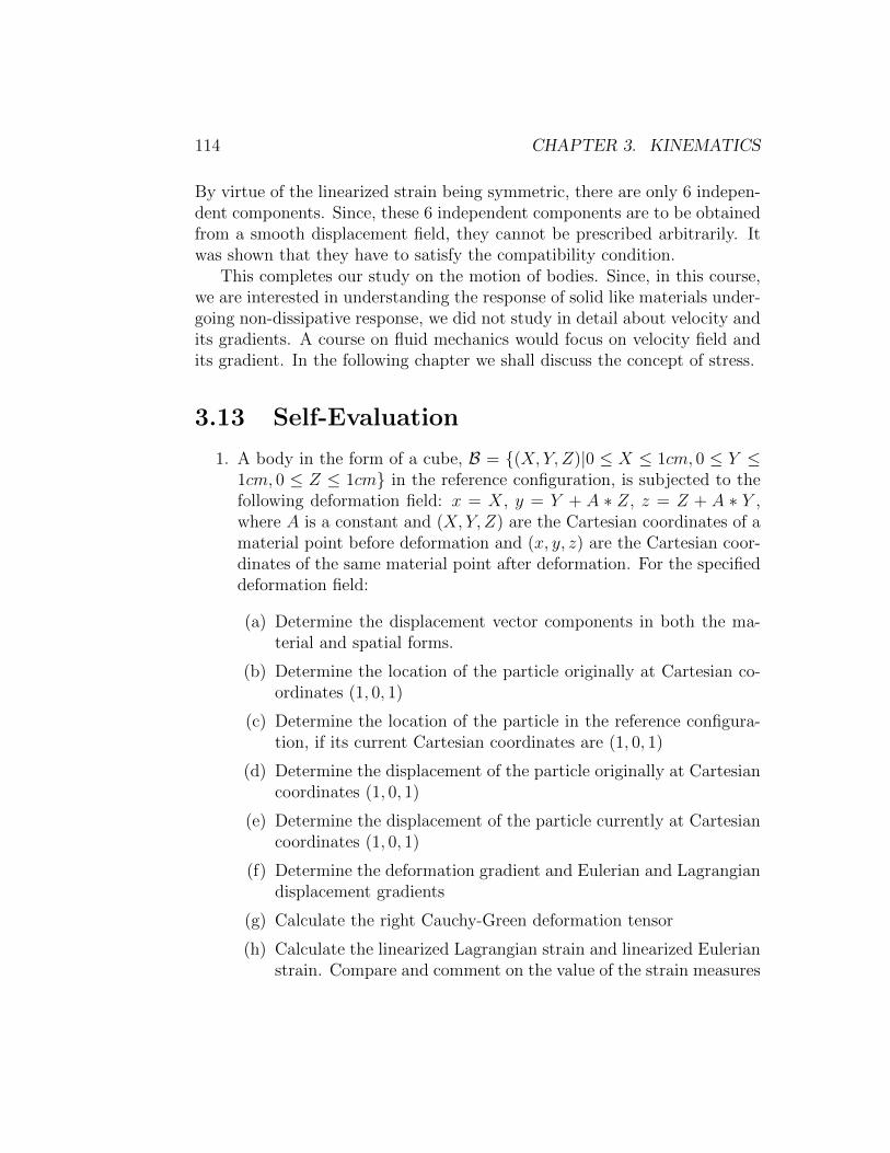
114 CHAPTER 3. KINEMATICS
By virtue of the linearized strain being symmetric, there are only 6 indepen-dent components. Since, these 6 independent components are to be obtainedfrom a smooth displacement field, they cannot be prescribed arbitrarily. Itwas shown that they have to satisfy the compatibility condition.
This completes our study on the motion of bodies. Since, in this course,we are interested in understanding the response of solid like materials under-going non-dissipative response, we did not study in detail about velocity andits gradients. A course on fluid mechanics would focus on velocity field andits gradient. In the following chapter we shall discuss the concept of stress.
3.13 Self-Evaluation
1. A body in the form of a cube, B = (X, Y, Z)|0 ≤ X ≤ 1cm, 0 ≤ Y ≤1cm, 0 ≤ Z ≤ 1cm in the reference configuration, is subjected to thefollowing deformation field: x = X, y = Y + A ∗ Z, z = Z + A ∗ Y ,where A is a constant and (X, Y, Z) are the Cartesian coordinates of amaterial point before deformation and (x, y, z) are the Cartesian coor-dinates of the same material point after deformation. For the specifieddeformation field:
(a) Determine the displacement vector components in both the ma-terial and spatial forms.
(b) Determine the location of the particle originally at Cartesian co-ordinates (1, 0, 1)
(c) Determine the location of the particle in the reference configura-tion, if its current Cartesian coordinates are (1, 0, 1)
(d) Determine the displacement of the particle originally at Cartesiancoordinates (1, 0, 1)
(e) Determine the displacement of the particle currently at Cartesiancoordinates (1, 0, 1)
(f) Determine the deformation gradient and Eulerian and Lagrangiandisplacement gradients
(g) Calculate the right Cauchy-Green deformation tensor
(h) Calculate the linearized Lagrangian strain and linearized Eulerianstrain. Compare and comment on the value of the strain measures

3.13. SELF-EVALUATION 115
(i) Calculate the change in the angle between two line segments ini-tially oriented along Ey and Ez directions in the reference config-uration
(j) Calculate the change in the volume of the cube
(k) Calculate the deformed surface area and its orientation for eachof the six faces of a cube
(l) Calculate the change in length of the straight line segments oflength 1 mm initially oriented along (i) Ey (ii) Ez (iii) (Ey +Ez)/
√2
(m) Is the motion field realizable for any value of A in the cube? Jus-tify. If not, find the values that A can take.
(n) Determine the displaced location of the material particles whichoriginally comprise
(i) The plane circular surface X = 0, Y 2 + Z2 = 0.25,
(ii) The plane elliptical surface X = 0, 9Y 2 + 4Z2 = 1.
(iii) The plane elliptical surface X = 0, 4Y 2 + 9Z2 = 1.
(o) Sketch the displaced configurations for (i), (ii) and (iii) in theabove problem if A = 0.1.
(p) Sketch the deformed configuration of the cube assuming A = 0.1.
2. Rework the parts (a) to (p) in the above problem if the cube is subjectedto a displacement field of the form, u = (A ∗ Y + 2A ∗ Z)ey + (3A ∗Y − A ∗ Z)ez, where (X, Y, Z) denotes the coordinates of a typicalmaterial particle in the reference configuration and ei the Cartesiancoordinate basis.
3. Which of the following displacement fields of a cube is homogeneous?
(a) u = A ∗ Zey + A ∗ Zez, where A is a constant
(b) u = [(cos(θ)− 1)X + sin(θ)Y ]ex + [− sin(θ)X + (cos(θ)− 1)Y ]ey,where θ is some constant
(c) u = 3XY 2ex + 2XZey + (Z2 −XY )ez
Here as usual (X, Y, Z) denotes the coordinates of a typical materialparticle in the reference configuration and ei the Cartesian coordinatebasis. For these deformation fields find parts (a) to (l) in problem 1.
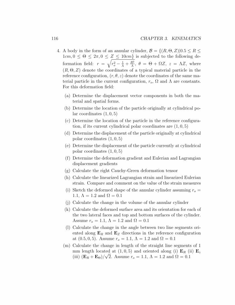
116 CHAPTER 3. KINEMATICS
4. A body in the form of an annular cylinder, B = (R,Θ, Z)|0.5 ≤ R ≤1cm, 0 ≤ Θ ≤ 2π, 0 ≤ Z ≤ 10cm is subjected to the following de-
formation field: r =√r2o − 1
Λ+ R2
Λ, θ = Θ + ΩZ, z = ΛZ, where
(R,Θ, Z) denote the coordinates of a typical material particle in thereference configuration, (r, θ, z) denote the coordinates of the same ma-terial particle in the current configuration, ro, Ω and Λ are constants.For this deformation field:
(a) Determine the displacement vector components in both the ma-terial and spatial forms.
(b) Determine the location of the particle originally at cylindrical po-lar coordinates (1, 0, 5)
(c) Determine the location of the particle in the reference configura-tion, if its current cylindrical polar coordinates are (1, 0, 5)
(d) Determine the displacement of the particle originally at cylindricalpolar coordinates (1, 0, 5)
(e) Determine the displacement of the particle currently at cylindricalpolar coordinates (1, 0, 5)
(f) Determine the deformation gradient and Eulerian and Lagrangiandisplacement gradients
(g) Calculate the right Cauchy-Green deformation tensor
(h) Calculate the linearized Lagrangian strain and linearized Eulerianstrain. Compare and comment on the value of the strain measures
(i) Sketch the deformed shape of the annular cylinder assuming ro =1.1, Λ = 1.2 and Ω = 0.1
(j) Calculate the change in the volume of the annular cylinder
(k) Calculate the deformed surface area and its orientation for each ofthe two lateral faces and top and bottom surfaces of the cylinder.Assume ro = 1.1, Λ = 1.2 and Ω = 0.1
(l) Calculate the change in the angle between two line segments ori-ented along ER and EZ directions in the reference configurationat (0.5, 0, 5). Assume ro = 1.1, Λ = 1.2 and Ω = 0.1
(m) Calculate the change in length of the straight line segments of 1mm length located at (1, 0, 5) and oriented along (i) ER (ii) Ez
(iii) (ER + EΘ)/√
2. Assume ro = 1.1, Λ = 1.2 and Ω = 0.1
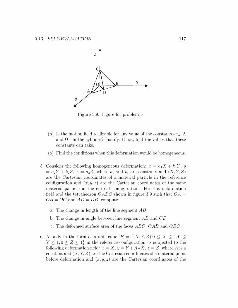
3.13. SELF-EVALUATION 117
Y
X
Z
B
C
A D D
O
Figure 3.9: Figure for problem 5
(n) Is the motion field realizable for any value of the constants - ro, Λand Ω - in the cylinder? Justify. If not, find the values that theseconstants can take.
(o) Find the conditions when this deformation would be homogeneous.
5. Consider the following homogeneous deformation: x = a1X + k1Y , y= a2Y + k2Z, z = a3Z, where ai and ki are constants and (X, Y, Z)are the Cartesian coordinates of a material particle in the referenceconfiguration and (x, y, z) are the Cartesian coordinates of the samematerial particle in the current configuration. For this deformationfield and the tetrahedron OABC shown in figure 3.9 such that OA =OB = OC and AD = DB, compute
a. The change in length of the line segment AB
b. The change in angle between line segment AB and CD
c. The deformed surface area of the faces ABC, OAB and OBC
6. A body in the form of a unit cube, B = (X, Y, Z)|0 ≤ X ≤ 1, 0 ≤Y ≤ 1, 0 ≤ Z ≤ 1 in the reference configuration, is subjected to thefollowing deformation field: x = X, y = Y +A∗X, z = Z, where A is aconstant and (X, Y, Z) are the Cartesian coordinates of a material pointbefore deformation and (x, y, z) are the Cartesian coordinates of the

118 CHAPTER 3. KINEMATICS
same material point after deformation. For the specified deformationfield:
(a) Compute the right Cauchy-Green deformation tensor
(b) Compute the linearized Lagrangian strain tensor
(c) Compute the eigenvalues and eigenvectors for right Cauchy-Greendeformation tensor
(d) Compute the eigenvalues and eigenvectors for linearized strain ten-sor
(e) Find the direction of the line segments in the reference configu-ration along which the maximum extension or shortening occursand its value
(f) Find the directions of the line segments in the reference configu-ration along which no extension or shortening takes place in thecube
(g) Find the maximum change in angle between line segments and theorientation of the line segments for which this occurs.
(h) Find the directions orthogonal to planes in which no change ofarea occurs
(i) Find the change in volume of the cube
(j) Decompose deformation gradient, F as F = RU, where R is theproper orthogonal tensor and U is a symmetric positive definitetensor.
7. A body in the form of a unit cube, B = (X, Y, Z)|0 ≤ X ≤ 1, 0 ≤Y ≤ 1, 0 ≤ Z ≤ 1 in the reference configuration, is subjected to thefollowing linearized strain field:
ε =
AY 3 +BX2 CXY (X + Y ) 0CXY (X + Y ) AX3 +DY 0
0 0 0
, (3.142)
where A, B, C, D are constants, find conditions, if any, on the con-stants if this strain field is to be obtained from a smooth displacementfield of the cube. For this value of the constants, find the smooth dis-placement field that gives raise to the above linearized strain field in a

3.13. SELF-EVALUATION 119
cube. Assume the coordinates of the point (0, 0, 0) after deformation is(10, 0, 0) and that of the point (0, 0, 1) after deformation is (10, 0, 1) todetermine the unknown constants in the displacement field. For whatmagnitude of these constants is the use of linearized strain justified.
8. A cube of side 10 cm, is subjected to a uniform plane state of strainwhose Cartesian components are:
ε =
1 −2 0−2 3 00 0 0
∗ 10−4. (3.143)
For this constant strain field, find
(a) Eigenvalues and eigenvectors of this strain tensor
(b) Maximum change in length and the direction of the material fiberalong which this occurs
(c) Maximum change in angle and the orientation of the materialfibers along which this occurs
(d) Whether the deformation is isochoric
(e) Change in length of a material fiber oriented along (ex + ey)/√
2and of length 1 mm
(f) Change in angle between line elements oriented along (ex+ey)/√
2and (ex − ey)/
√2
9. A rosette strain gauge is an electromechanical device that can measurerelative surface elongations in three directions. Bonding such a deviceto the surface of a structure allows determination of elongation alongthe direction in which the gauge is located. Figure 3.10 shows theorientation of gauges in one such rosette along with the coordinatesystem used to study the problem. For a particular loading, thesegauges measured the strain along their directions as εa = 0.001, εb =0.002 and εc = 0.004. Assuming the state of strain at the point ofmeasurement is plane, find the Cartesian components of the strain:εxx, εyy and εxy for the orientation of the basis also shown in the figure3.10.
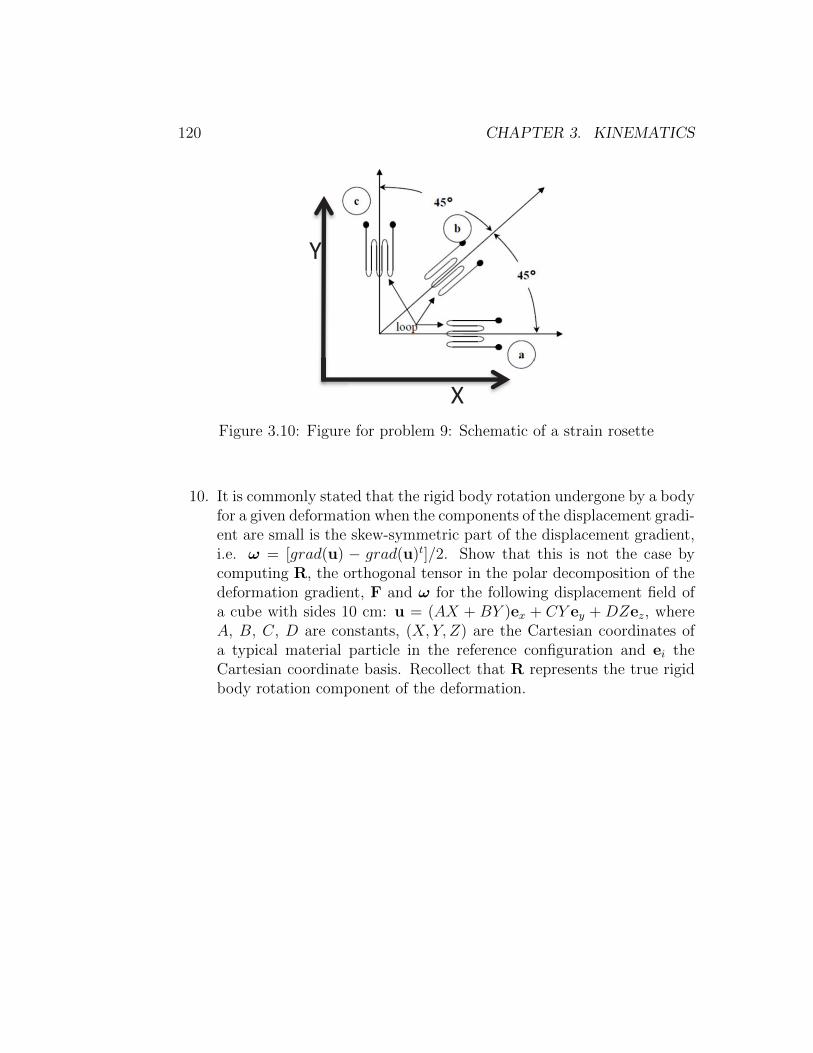
120 CHAPTER 3. KINEMATICS
Y
X Figure 3.10: Figure for problem 9: Schematic of a strain rosette
10. It is commonly stated that the rigid body rotation undergone by a bodyfor a given deformation when the components of the displacement gradi-ent are small is the skew-symmetric part of the displacement gradient,i.e. ω = [grad(u) − grad(u)t]/2. Show that this is not the case bycomputing R, the orthogonal tensor in the polar decomposition of thedeformation gradient, F and ω for the following displacement field ofa cube with sides 10 cm: u = (AX + BY )ex + CY ey + DZez, whereA, B, C, D are constants, (X, Y, Z) are the Cartesian coordinates ofa typical material particle in the reference configuration and ei theCartesian coordinate basis. Recollect that R represents the true rigidbody rotation component of the deformation.
Chapter 4
Traction and Stress
4.1 Overview
Mechanics is the branch of science that describes or predicts the state ofrest or of motion of bodies subjected to some forces. In the last chapter, westudied about mathematical descriptors of the state of rest or of motion ofbodies. Now, we shall focus on the cause for motion or change of geometryof the body; the force. While in rigid body mechanics, the concept of force issufficient to describe or predict the motion of the body, in deformable bodiesit is not. For example, two bars made of the same material and of samelength but with different cross sectional area, will undergo different amountof elongation when subjected to the same pulling force acting parallel to theaxis of the bar. It was then found that if we define a quantity called strainwhich is defined as the ratio between the change in length to the originallength of the bar along the direction of the applied load and a quantitycalled stress which is defined as the force acting per unit area then the stressand strain could be related through an equation that is independent of thegeometry of the body but depend only on the material that the body ismade up of. While these definitions of strain and stress are adequate tostudy homogeneous deformations resulting from uniform stress states, theseconcepts have to be generalized to study the motion of bodies subjected to anon-uniform distribution of forces and/or couples. In this chapter, we shallgeneralize the concept of stress having already generalized the concept ofstrain in the last chapter.
121

122 CHAPTER 4. TRACTION AND STRESS
(a) External loads acting on a solid inequilibrium
(b) Internal loads acting on a plane pass-ing by O inside a solid
Figure 4.1: Free body diagram showing the forces acting on a body
4.2 Traction vectors and stress tensors
Here we focus attention on a deformable continuum body B occupying anarbitrary region Bt of the Euclidean vector space with boundary surface∂Bt at time t, as shown in figure 4.1a. We consider a general case where inarbitrary forces act on parts or the whole of the boundary surface called theexternal forces or loads. Recognizing that these external forces arose becausewe isolated the body from its surroundings, to find the internal forces we haveto section the body. Thus, to find the internal forces on a internal surfacepassing through O, as indicated in the figure 4.1a, we have to section thebody as shown in the figure 4.1b, with the cutting plane coinciding with the

4.2. TRACTION VECTORS AND STRESS TENSORS 123
t(n) n
t(n)n
o
o
Figure 4.2: Traction vectors acting on infinitesimal surface elements withoutward unit normal, n
internal surface. Now, we focus our attention on an infinitesimal part of thebody centered around O, see figure 4.2. Let x be the position vector of thepoint O, n a unit vector directed along the outward normal to an infinitesimalspatial surface element ∆s, at x and ∆f denote the infinitesimal resultantforce acting on the surface element ∆s. Then, we claim that
∆f =
∫∆s
t(n)da, (4.1)
where t(n) = t(x, t,n) represents the Cauchy (or true) traction vector and theintegration here denotes an area integral. Thus, Cauchy traction vector isthe force per unit surface area defined in the current configuration acting at agiven location. The Cauchy traction vector and hence the infinitesimal forceat a given location depends also on the orientation of the cutting plane, i.e.,the unit normal n. This means that the traction and hence the infinitesimalforce at the point O, for a vertical cutting plane could be different from thatof a horizontal cutting plane. However, the traction on the two pieces of thecut body would be such that they are equal in magnitude but opposite indirection, in order to satisfy Newton’s third law of motion. Hence,
t(n) = −t(−n). (4.2)
This requires: t(x, t,n) = −t(x, t,−n).

124 CHAPTER 4. TRACTION AND STRESS
Relationship (4.1) is referred to as Cauchy’s postulate. It is worthwhileto mention that in any experiment we infer only these traction vectors. Inliterature, the traction vector is also called as stress vector because they havethe units of stress, i.e., force per unit area. However, here we shall not usethis terminology and for us stress is always a tensor, as defined next.
4.2.1 Cauchy stress theorem
There exist unique second order tensor field σ, called the Cauchy (or true)stress tensor, so that
t(n) = t(x, t,n) = σtn. (4.3)
where σ = σ(x, t) = σ(X, t), X ∈ Br, is the position vector of the materialparticle in the reference configuration. It is easy to verify that the require-ment (4.2) is met by (4.3). It will be shown in the next chapter that theCauchy stress tensor, σ has to be a symmetric tensor. However, the proof ofCauchy stress theorem is beyond the scope of these lecture notes.
4.2.2 Components of Cauchy stress
It is recalled that only traction vector can be determined or inferred in theexperiments and hence the components of the stress tensor is estimated fromfinding the traction vector on three (mutually perpendicular) planes. Let ussee how.
The components of the Cauchy stress tensor, σ with respect to an or-thonormal basis ea is given by:
σab = ea · σeb = σtea · eb = t(ea) · eb, (4.4)
In view of Cauchy’s theorem t(ea) = σtea, a = 1, 2, 3, characterize the threetraction vectors acting on the surface elements whose outward normals pointin the directions e1, e2, e3, respectively. Then, the components of thesetraction vectors along e1, e2, e3 gives the various components of the stresstensor. Thus, for each stress component σab we adopt the mathematicallylogical convention that the index b characterizes the component of the trac-tion vector, t(ea), at a point x in the direction of the associated base vectoreb and the index a characterizes the orientation of the area element on whicht(n) is acting.

4.2. TRACTION VECTORS AND STRESS TENSORS 125
xx
x
y
z
xy
xx
xy
yx
yx zx
zx
xz
xz
zy
zy
yz yz
yy
yy
zz
zz
Figure 4.3: Cartesian components of the stress tensor acting on the faces ofa cube
It is important to note that some authors reverse this convention byidentifying the index b with the orientation of the normal to the plane ofcut and the index a with the component of the traction along the directionea. Irrespective of the convention adopted the end results will be the samebecause of two reasons: (i) The definition of divergence is suitably modifiedwith a transpose (ii) the Cauchy stress tensor is anyway symmetric. In otherwords, to find the components of the Cauchy stress tensor, at a given location,we isolate an infinitesimal cube with the location of interest at its center.The cube is oriented such that the outward normal to its sides is along oropposite to the direction of the basis vectors. Hence, for general curvilinearcoordinates, the sides of the cube need not be plane nor make right angleswith each other. Compare the stress cube for Cartesian basis (figure 4.3) andcylindrical polar basis (figure 4.4). Then, we determine the traction that isacting on each of the six faces of the cube. Due to equation (4.2) only threeof these six traction vectors are independent. The components of the threetraction vectors along the the three basis vectors gives the nine componentsof the stress tensor.
If the component of the traction is along the direction of the basis vectorson planes whose outward normal coincides with the direction of the basis

126 CHAPTER 4. TRACTION AND STRESS
dz
r dθ
dr
Figure 4.4: Cylindrical polar basis components of the stress tensor acting onthe faces of a cube
vectors it is considered to be positive and negative otherwise. Consistently,if the component of the traction is opposite to the direction of the basisvectors on faces of the cube whose outward normal is opposite in directionto the basis vectors, it is considered to be positive and negative otherwise.Thus, one should not be confused that the same stress component points inopposite directions on opposite planes. This is necessary for the cube underconsideration to be in equilibrium. It should also be appreciated that thesign of some of the stress component does change when the direction of thecoordinate basis is reversed even if the right handedness of the basis vectorsis maintained. This is so, because the sign of the stress component dependsboth on the direction of coordinate basis as well as the outward normal.Thus, figure 4.3 portrays the positive components of the stress tensor whenCartesian coordinate basis is used and it is called as the stress cube.
The positive cylindrical polar components of the stress tensor is depictedon a cylindrical wedge in figure 4.4. Recognize that the direction of thecylindrical polar components of the stress changes with the location unlike theCartesian coordinate components whose directions are fixed. This happensbecause the direction of the cylindrical polar coordinate basis vectors dependson the location. Here σrr component of the stress is called as the radial stress,

4.3. NORMAL AND SHEAR STRESSES 127
σθθ component of the stress is known as the hoop or the circumferential stress,σzz component of the stress is the axial stress.
4.3 Normal and shear stresses
Let the traction vector t(n) for a given current position x at time t act on anarbitrarily oriented surface element characterized by an outward unit normalvector n.
The traction vector t(n) may be resolved into the sum of a vector along
the normal n to the plane, denoted by t‖(n) and a vector perpendicular to n
denoted by t⊥(n), i.e., t(n) = t‖(n) + t⊥(n). From the results in section 2.3.3, it
could be seen that
t‖(n) = [n · t(n)]n = [n · σn]n = σnn, (4.5)
t⊥(n) = t(n) − [n · t(n)]n = [1− n⊗ n]t(n) = τnm, (4.6)
where
τn = | t(n) − [n · t(n)]n |=| σn− [n · σn]n |, (4.7)
m =1
τnt(n) − [n · t(n)]n. (4.8)
It could easily be verified that n ·m = 0. This means m is a vector embeddedin the surface. Then, σn is called the normal traction and τn is called theshear traction. As the names suggest, normal traction acts perpendicular tothe surface and shear traction acts tangential or parallel to the surface.
Since, t(n) = t‖(n) + t⊥(n), we obtain the useful relation
| t(n) |2= σ2n + τ 2
n, (4.9)
where we have made use of the property that n ·m = 0.It could be seen from figure 4.3 that the stress components corresponding
to Cartesian basis, σxx, σyy and σzz act normal to their respective surfacesand hence are called normal stresses and the remaining independent com-ponents, σxy, σyz and σzx act parallel to the surface and hence are calledshear stresses. (Remember that Cauchy stress is a symmetric tensor.) Whenthe stress components are determined with respect to any coordinate basisvectors, there will be three normal stresses corresponding to σii and three

128 CHAPTER 4. TRACTION AND STRESS
shear stresses, σij, i 6= j. Here to call certain components of the stresses asnormal and others as shear, we have exploited the relationship between thecomponents of the stress tensor and the traction vector.
4.4 Principal stresses and directions
At a given location in the body the magnitude of the normal and sheartraction depend on the orientation of the plane. An isotropic body can failalong any plane and hence we require to find the maximum magnitude ofthese normal and shear traction and the planes for which these occur. As weshall see on planes where the maximum or minimum normal stresses occurthe shear stresses are zero. However, in the plane on which maximum shearstress occurs, the normal stresses will exist.
4.4.1 Maximum and minimum normal traction
In order to obtain the maximum and minimum values of σn, the normaltraction, we have to find the orientation of the plane in which this occurs.This is done by maximizing (4.5) subject to the constraint that | n | = 1. Thisconstrained optimization is done by what is called as the Lagrange-multipliermethod. Towards this, we introduce the function
L(n, λ∗) = n · σn− λ∗[| n |2 −1], (4.10)
where λ∗ is the Lagrange multiplier and the condition | n |2 − 1 = 0 char-acterizes the constraint condition. At locations where the extremal values ofL occurs, the derivatives ∂L
∂nand ∂L
∂λ∗must vanish, i.e.,
∂L∂n
= 2(σn− λ∗n) = o, (4.11)
∂L∂λ∗
= | n |2 −1 = 0. (4.12)
To obtain these equations we have made use of the fact that Cauchy stresstensor is symmetric. Thus, we have to find three na and λ∗a’s such that
(σ − λ∗a1)na = o, | na |2= 1, (4.13)
(a = 1, 2, 3; no summation) which is nothing but the eigenvalue probleminvolving the tensor σ with the Lagrange multiplier being identified as the
4.4. PRINCIPAL STRESSES AND DIRECTIONS 129
eigenvalue. Hence, the results of section 2.5 follows. In particular, for (4.13a)to have a non-trivial solution
λ∗3a −K1λ∗2a +K2λ
∗a −K3 = 0, (4.14)
where
K1 = tr(σ), K2 =1
2[K2
1 − tr(σ2)], K3 = det(σ), (4.15)
the principal invariants of the stress σ. As stated in section 2.5, equation(4.14) has three real roots, since the Cauchy stress tensor is symmetric. Theseroots (λ∗a) will henceforth be denoted by σ1, σ2 and σ3 and are called principalstresses. The principal stresses include both the maximum and minimumnormal stresses among all planes passing through a given x.
The corresponding three orthonormal eigenvectors na, which are thencharacterized through the relation (4.13) are called the principal directionsof σ. The planes for which these eigenvectors are normal are called principalplanes. Further, these eigenvectors form a mutually orthogonal basis sincethe stress tensor σ is symmetric. This property of the stress tensor alsoallows us to represent σ in the spectral form
σ =3∑
a=1
σana ⊗ na. (4.16)
It is immediately apparent that the shear stresses in the principal planes arezero. Thus, principal planes can also be defined as those planes in which theshear stresses vanish. Consequently, σa’s are normal stresses.
4.4.2 Maximum and minimum shear traction
Next, we are interested in finding the direction of the unit vector n at xthat gives the maximum and minimum values of the shear traction, τp. Thisis important because in many metals the failure is due to sliding of planesresulting due to the shear traction exceeding a critical value along some plane.
In the following we choose the eigenvectors na of σ as the set of basisvectors. Then, according to the spectral decomposition (4.16), all the non-diagonal matrix components of the Cauchy stress vanish. Then, the tractionvector t(p) on an arbitrary plane with normal p could simply be written as
t(p) = σp = σ1p1n1 + σ2p2n2 + σ3p3n3, (4.17)

130 CHAPTER 4. TRACTION AND STRESS
where p = p1n1 + p2n2 + p3n3. It then follows from (4.9) that
τ 2p = | t(p) |2 −σ2
p
= σ21p
21 + σ2
2p22 + σ2
3p23 − (σ1p
21 + σ2p
22 + σ3p
23)2, (4.18)
where σp is the normal traction on the plane whose normal is p.
With the constraint condition | p |2 = 1 we can eliminate p3 from theequation (4.18). Then, since the principal stresses, σ1, σ2, σ3 are known, τ 2
p
is a function of only p1 and p2. Therefore to obtain the extremal values of τ 2p
we differentiate τ 2p with respect to p1 and p2 and equate it to zero1:
∂τ 2p
∂p1
= 2p1[σ1 − σ3]σ1 − σ3 − 2[(σ1 − σ3)p21 + (σ2 − σ3)p2
2] = 0, (4.19)
∂τ 2p
∂p2
= 2p2[σ2 − σ3]σ2 − σ3 − 2[(σ1 − σ3)p21 + (σ2 − σ3)p2
2] = 0. (4.20)
The above set of equations has three classes of solutions.
• Set - 1: p1 = p2 = 0 and hence p3 = ±1, obtained from the conditionthat | p |2 = 1.
• Set - 2: p1 = 0, p2 = ±1/√
2 and hence p3 = ±1/√
2.
• Set - 3: p1 = ±1/√
2, p2 = 0 and hence p3 = ±1/√
2.
Instead of eliminating p3 we could eliminate p2 or p1 initially and find theremaining unknowns by adopting a procedure similar to the above. Then,we shall find the extremal values of τp could also occur when
• Set - 4: p1 = p3 = 0 and hence p2 = ±1.
• Set - 5: p2 = p3 = 0 and hence p1 = ±1.
• Set - 6: p3 = 0, p1 = ±1/√
2 and hence p2 = ±1/√
2.
1Recognize that the extremal values of both τp and τ2p occur at the same location.
4.5. STRESSES ON A OCTAHEDRAL PLANE 131
Substituting these solutions in (4.18) we find the extremal values of τp. Thus,τp = 0 when p = ±n1 or p = ±n2 or p = ±n3 and
p = ± 1√2n2 ±
1√2n3, τ 2
p =1
4(σ2 − σ3)2, (4.21)
p = ± 1√2n1 ±
1√2n3, τ 2
p =1
4(σ1 − σ3)2, (4.22)
p = ± 1√2n1 ±
1√2n2, τ 2
p =1
4(σ1 − σ2)2. (4.23)
Consequently, the maximum magnitude of the shear traction denoted byτmax is given by the largest of the three values of (4.21b) - (4.23b). Thus, weobtain
τmax =1
2(σmax − σmin), (4.24)
where σmax and σmin denote the maximum and minimum magnitudes of prin-cipal stresses, respectively. Recognize that the maximum shear stress acts ona plane that is shifted about an angle of ±45 degrees to the principal planein which the maximum and minimum principal stresses act. In addition, wecan show that the normal traction σp to the plane in which τmax occurs hasthe value σp = (σmax + σmin)/2.
4.5 Stresses on a Octahedral plane
Consider now a tetrahedron element similar to that of figure 4.5 with a planeequally inclined to the principal axes. Hence, its normal is given by
p = ± 1√3n1 ±
1√3n2 ±
1√3n3, (4.25)
where na are the three principal directions of the Cauchy stress tensor. Then,the normal traction, σoct, on this plane is
σoct =1
3[σ1 + σ2 + σ3], (4.26)
obtained using (4.5) and the spectral representation for the Cauchy stress(4.16). Similarly, the shear traction, τoct on this plane is
τ 2oct =
1
3[σ2
1 + σ22 + σ2
3]− 1
9(σ1 + σ2 + σ3)2. (4.27)

132 CHAPTER 4. TRACTION AND STRESS
Figure 4.5: Eight octahedral planes equally inclined to the principal axes.
From the definition of principal invariants for stress (4.15) it is easy to verifythat
σoct =K1
3, τoct =
2
9K2
1 −2
3K2. (4.28)
Using the above formula one can compute the octahedral normal and sheartraction for stress tensor represented using some arbitrary basis.
4.6 Examples of state of stress
Specifying a state of stress means providing sufficient information to computethe components of the stress tensor with respect to some basis. As discussedbefore, knowing t(n) for three independent pairs of t(n),n we can constructthe stress tensor σ. Hence, specifying the set of pairs (t(n),n) for threeindependent normal vectors, n, at a given point, so that the stress tensorcould be uniquely determined tantamount to prescribing the state of stress.Next, we shall look at some states of stress.
The state of stress is said to be uniform if the stress tensor does not
4.6. EXAMPLES OF STATE OF STRESS 133
depend on the space coordinates at each time t, when the stress tensor isrepresented using Cartesian basis vectors.
If the stress tensor has a representation
σ = σn⊗ n, (4.29)
at some point, where n is a unit vector, we say it is in a pure normal stressstate. Post-multiplying (4.29) with the unit vector n we find that
σn = σ(n⊗ n)n = σ(n · n)n = σn = t‖n. (4.30)
Evidently, the traction is along (or opposite to) n. This stress σ characterizeseither pure tension (if σ > 0) or pure compression (if σ < 0).
If we have a uniform stress state and the stress tensor when representedusing a Cartesian basis is such that σxx = σ = const and all other stress com-ponents are zero, then such a stress state is referred to as uniaxial tension oruniaxial compression depending on whether σ is positive or negative respec-tively. This may be imagined as the stress in a rod with uniform cross-sectiongenerated by forces applied to its plane ends in the x − direction. However,recognize that this is not the only system of forces that would result in theabove state of stress; all that we require is that the resultant of a system offorces should be oriented along the ex direction.
If the stress tensor has a representation
σ = σ(n⊗ n + m⊗m), (4.31)
at any point, where n and m are unit vectors such that n ·m = 0, then it issaid to be in equibiaxial stress state.
On the other hand, if the stress tensor has a representation
σ = τ(n⊗m + m⊗ n), (4.32)
at any point, where n and m are unit vectors such that n ·m = 0, then it issaid to be in pure shear stress state. Post-multiplying (4.32) with the unitvector n we obtain
σn = τ(n⊗m + m⊗ n)n
= τ [(m · n)n + (n · n)m] = τm = t⊥m. (4.33)
Evidently, t⊥m is tangential to the surface whose outward unit normal is along(or opposite to) n.

134 CHAPTER 4. TRACTION AND STRESS
More generally, if the stress tensor has a representation
σ = σ1n⊗ n + σ2m⊗m, (4.34)
at any point, where n and m are unit vectors such that n ·m = 0, then itis said to be in plane or biaxial state of stress. That is in this case one ofthe principal stresses is zero. A general matrix representation for the stresstensor corresponding to a plane stress state is:
σ =
σ11 σ12 0σ12 σ22 00 0 0
. (4.35)
Here we have assumed that e3 is a principal direction and that there existno stress components along this direction. We could have assumed the samewith respect to any one of the other basis vectors. A plane stress state occursat any unloaded surface in a continuum body and is of practical interest.
Next, we consider 3D stress states. Analogous to the equibiaxial stressstate in 2D, if the stress tensor has a representation
σ = −p1, (4.36)
at some point, we say that it is in a hydrostatic state of stress and p is called ashydrostatic pressure. It is just customary to consider compressive hydrostaticpressure to be positive and hence the negative sign. Post-multiplying (4.36)by some unit vector n, we obtain
σn = (−p1)n = −pn = t‖n. (4.37)
Thus, on any surface only normal traction acts, which is characteristic of(elastic) fluids at rest that is not able to sustain shear stresses. Hence, thisstress is called hydrostatic.
Any other state of stress is called to be triaxial stress state.Many a times the stress is uniquely additively decomposed into two parts
namely an hydrostatic component and a deviatoric component, that is
σ =1
3tr(σ)1 + σdev. (4.38)
Thus, the deviatoric stress is by definition,
σdev = σ − 1
3tr(σ)1, (4.39)
4.7. OTHER STRESS MEASURES 135
and has the property that tr(σdev) = 0. Physically the hydrostatic compo-nent of the stress is supposed to cause volume changes in the body and thedeviatoric component cause distortion in the body. (Shear deformation is akind of distortional deformation.)
4.7 Other stress measures
Till now, we have been looking only at the Cauchy (or true) stress. As itsname suggest this is the “true” measure of stress. However, there are manyother definition of stresses but all of these are propounded just to facilitateeasy algebra. Except for the first Piola-Kirchhoff stress, other stress measuresdo not have a physical interpretation as well.
4.7.1 Piola-Kirchhoff stress tensors
Let ∂Ωt denote some surface within or on the boundary of the body in thecurrent configuration. Then, the net force acting on this surface is given by
f =
∫∂Ωt
t(n)da =
∫∂Ωt
σnda. (4.40)
It is easy to compute the above integral when the Cauchy stress is expressedas a function of x, the position vector of a typical material point in the currentconfiguration, i.e. σ = σ(x, t). On the other hand computing the aboveintegral becomes difficult when the stress is a function of X, the positionvector of a typical material point in the reference configuration, i.e. σ =σ(X, t). To facilitate the computation of the above integral in the later case,we appeal to the Nanson’s formula (3.72) to obtain
f =
∫∂Ωt
t(n)da =
∫∂Ωt
σnda =
∫∂Ωr
det(F)σF−tNdA, (4.41)
where ∂Ωr is the surface in the reference configuration, formed by the samematerial particles that formed the surface ∂Ωt in the current configuration.Then, the first Piola-Kirchhoff stress, P is defined as
P = det(F)σF−t. (4.42)

136 CHAPTER 4. TRACTION AND STRESS
Using this definition of Piola-Kirchhoff stress, equation (4.41) can be writtenas
f =
∫∂Ωt
σnda =
∫∂Ωr
PNdA. (4.43)
Assuming, the stress to be uniform over the surface of interest and the stateof stress corresponds to pure normal stress, it is easy to see that while Cauchystress is force per unit area in the current configuration, Piola-Kirchhoff stressis force per unit area in the reference configuration. This is the essentialdifference between the Piola-Kirchhoff stress and Cauchy stress. Recognizethat in both the cases the force acts only in the current configuration. In lieuof this Piola-Kirchhoff stress is a two-point tensor, similar to the deformationgradient, in that it is a linear transformation that relates the unit normal tothe surface in the reference configuration to the traction acting in the currentconfiguration. Thus, if Ea denote the three Cartesian basis vectors usedto describe the reference configuration and ea denote the Cartesian basisvectors used to describe the current configuration, then the Cauchy stressand Piola-Kirchhoff stress are represented as
σ = σabea ⊗ eb, P = PaBea ⊗ EB. (4.44)
We had mentioned earlier that the Cauchy stress tensor is symmetric forreasons to be discussed in the next chapter. Since, σ = PFt/ det(F), thesymmetric restriction on Cauchy stress tensor requires the Piola-Kirchhoffstress to satisfy the relation
PFt = FPt. (4.45)
Consequently, in general P is not symmetric and has nine independent com-ponents.
During an experiment, it is easy to find the surface areas in the referenceconfiguration and determine the traction or forces acting on these surfacesas the experiment progresses. Thus, Piola-Kirchhoff stress is what could bedirectly determined. Also, it is the stress that is reported, in many cases. TheCauchy stress is then obtained using the equation (4.42) from the estimateof the Piola-Kirchhoff stress and the deformation of the respective surface.
Further, since in solid mechanics, the coordinates of the material particlesin the reference configuration is used as independent variable, first Piola-Kirchhoff stress plays an important role in formulating the boundary valueproblem as we shall see in the ensuing chapters.

4.8. SUMMARY 137
The transpose of the Piola-Kirchhoff stress, Pt, is called as engineeringstress or nominal stress.
Another stress measure called the second Piola-Kirchhoff stress, S definedas
S = det(F)F−1σF−t = F−1P (4.46)
is used in some studies. Note that this tensor is symmetric and hence itsutility.
4.7.2 Kirchhoff, Biot and Mandel stress measures
Next, we define a few stress measures popular in literature. It is easy toestablish their inter-relationship and properties which we leave it as an exer-cise.
The Kirchhoff stress tensor, τ is defined as: τ = det(F)σ.The Biot stress tensor, TB also called material stress tensor is defined
as: TB = RtP, where R is the orthogonal tensor obtained during polardecomposition of F.
The co-rotated Cauchy stress tensor σu, introduced by Green and Naghdiis defined as: σu = RtσR.
The Mandel stress tensor, used often to describe inelastic response ofmaterials is defined as Σ = CS, where C is the right Cauchy-Green stretchtensor introduced in the previous chapter.
4.8 Summary
In this chapter, we introduced the concept of traction and stress tensor. Ifthe forces acting in the body are assumed to be distributed over the surfacesin the current configuration of the body, then the corresponding traction iscalled as Cauchy traction and the stress tensor associated with this tractionis called as the Cauchy stress tensor, σ. Similarly, if the forces acting inthe body is distributed over the surface in the reference configuration, thenthis traction is called as Piola traction and the stress tensor associated withthis traction the Piola-Kirchhoff stress, P. We also defined various types ofstresses like normal stress, shear stress, hydrostatic stress, octahedral stress.Having grasped the concepts of strain and stress we shall proceed to find therelation between the applied force and realized displacement in the followingchapters.
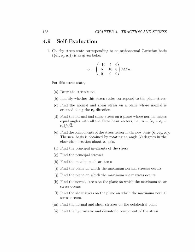
138 CHAPTER 4. TRACTION AND STRESS
4.9 Self-Evaluation
1. Cauchy stress state corresponding to an orthonormal Cartesian basis(ex, ey, ez) is as given below:
σ =
−10 5 05 10 00 0 0
MPa.
For this stress state,
(a) Draw the stress cube
(b) Identify whether this stress states correspond to the plane stress
(c) Find the normal and shear stress on a plane whose normal isoriented along the ex direction.
(d) Find the normal and shear stress on a plane whose normal makesequal angles with all the three basis vectors, i.e., n = (ex + ey +ez)/√
3.
(e) Find the components of the stress tensor in the new basis ex, ey, ez.The new basis is obtained by rotating an angle 30 degrees in theclockwise direction about ez axis.
(f) Find the principal invariants of the stress
(g) Find the principal stresses
(h) Find the maximum shear stress
(i) Find the plane on which the maximum normal stresses occurs
(j) Find the plane on which the maximum shear stress occurs
(k) Find the normal stress on the plane on which the maximum shearstress occurs
(l) Find the shear stress on the plane on which the maximum normalstress occurs.
(m) Find the normal and shear stresses on the octahedral plane
(n) Find the hydrostatic and deviatoric component of the stress

4.9. SELF-EVALUATION 139
2. Cauchy stress state corresponding to an orthonormal Cartesian basis(ex, ey, ez) is as given below:
σ =
−10 0 50 10 05 0 10
MPa.
For this stress state solve parts (a) through (n) in problem 1.
3. For the plane Cauchy stress state shown in figure 4.6, write the stresstensor and solve parts (b) through (n) in problem 1.
4. For the Cauchy stress cube shown in figure 4.7, write the stress tensorand solve parts (b) through (n) in problem 1.
5. An annular circular cylinder with deformed outer diameter 25 mm issubjected to a tensile force of 1200 N as shown in figure 4.8. Experi-ments revealed that a uniform axial true stress of 3.8 MPa has devel-oped due to this applied force. Using the above information, determinethe deformed inner diameter of the cylinder.
6. Three pieces of wood having 3.75 cm x 3.75 cm square cross-sectionsare glued together and to the foundation as shown in figure 4.9. If thehorizontal force P = 3, 000 N what is the average shearing engineeringstress in each of the glued joints?
7. Find the maximum permissible value of load P for the bolted jointshown in the figure 4.10, if the allowable shear stress in the bolt materialis 100 MPa. Bolts are 20 mm in diameter. List the assumptions in yourcalculation, if any.
8. Two wooden planks each 25 mm thick and 150 mm wide are joined bythe glued mortise joint shown in figure 4.11. Knowing that the jointwill fail when the average engineering shearing stress in the glue exceeds0.9 MPa, determine the smallest allowable length d of the cuts if thejoint is to withstand an axial load P that the planks would otherwiseresist if there were no joint. Assume that the wooden plank fails if theengineering axial stresses exceed 1.5 MPa.
9. Two wooden members of 90 x 140 mm uniform rectangular cross sec-tion are joined by the simple glued scarf splice shown in figure 4.12.
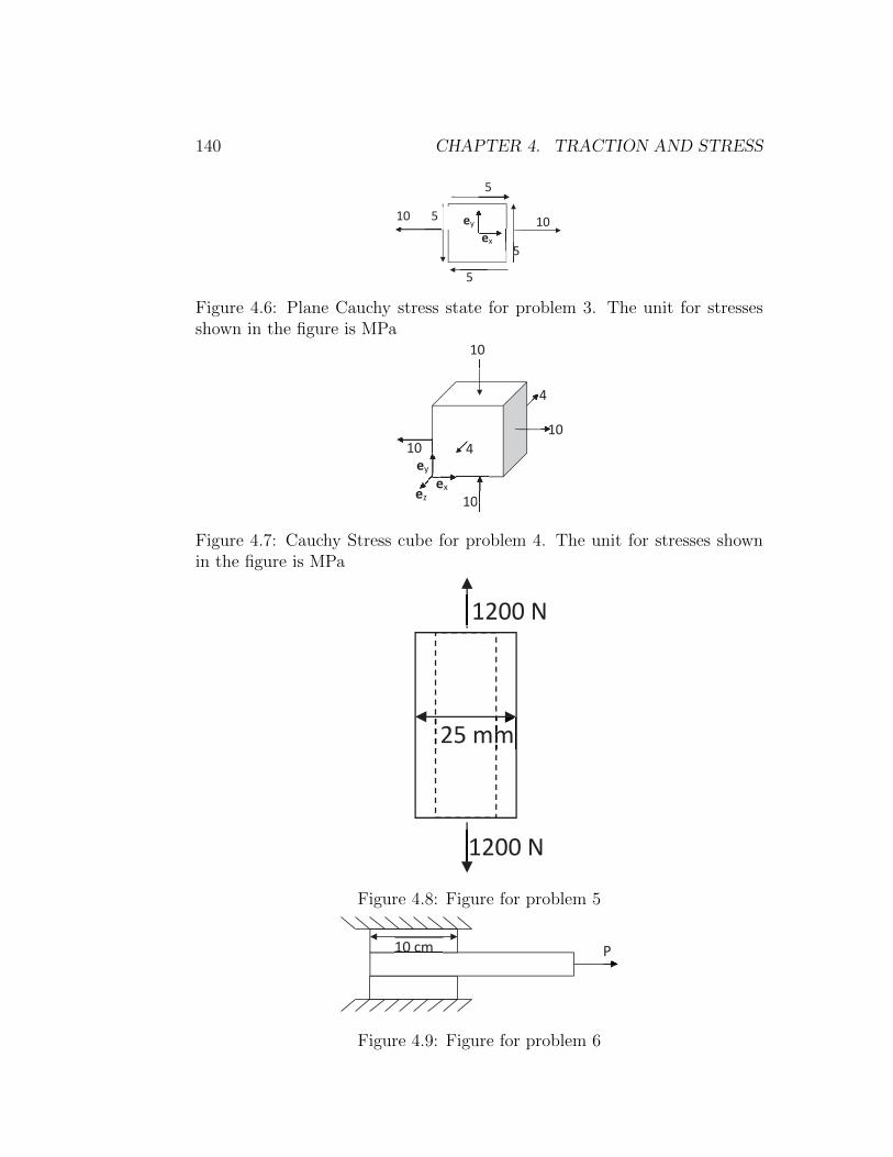
140 CHAPTER 4. TRACTION AND STRESS
10
5
5
5
5 10
5ex
ey
Figure 4.6: Plane Cauchy stress state for problem 3. The unit for stressesshown in the figure is MPa
10
10
10
10 4
4
10ex e
ey ee
ez
Figure 4.7: Cauchy Stress cube for problem 4. The unit for stresses shownin the figure is MPa
1200 N
1200 N
25 mm
Figure 4.8: Figure for problem 5
P 10 cm
Figure 4.9: Figure for problem 6

4.9. SELF-EVALUATION 141
75
P
50
P PPAll dimensions in mm
Figure 4.10: Figure for problem 7
150
20
20
d
Glue
P
Figure 4.11: Figure for problem 8

142 CHAPTER 4. TRACTION AND STRESS
20° P 90 mm
150 mm
Figure 4.12: Figure for problem 9
Knowing that the maximum allowable engineering shearing stress inthe glued splice is 0.75 MPa, determine the largest axial load P thatcan be safely applied as shown in figure 4.12.
10. A plate has been subjected to the following state of Cauchy stress:
σ =
−5 0 50 0 05 0 10
MPa,
where the components of the stress is with respect to an orthonor-mal Cartesian basis (ex, ey, ez). For this state of stress, answer thefollowing:
(a) Does this state of stress correspond to plane stress? Justify
(b) If the plate were to be made of reinforced concrete, find the di-rection(s) in which reinforcement needs to be provided. Recollectthat reinforcement is provided in concrete to resist tensile stresses.
(c) Find the additional σzz component of the stress that can be ap-plied, to the above plate, so that the maximum normal stress is230 MPa
(d) If the plate were to be made of wood, in which the grains orien-tation, m = 0.61ex + 0.50ey + 0.61ez and if the maximum shearstress that can be sustained along the orientation of the grains is20 MPa, determine if the wooden plate will fail for the above stateof stress.
(e) Now say, hydrostatic state of stress is applied in addition to theabove state of stress, find the hydrostatic pressure at which thewooden plate will fail, if it will.

Chapter 5
Balance Laws
5.1 Overview
The balance laws, discussed in this chapter, has to be satisfied for all bod-ies, irrespective of the material that they are made up of. The fundamentalbalance laws that would be discussed here are conservation of mass, linearmomentum, and angular momentum. However, the particular form thatthese equations take would depend on the processes that one is interestedin. Here our interest is in what is called as purely mechanical processes andhence we are not concerned about conservation of energy or electric charge ormagnetic flux. These general balance equations in themselves do not sufficeto determine the deformation or motion of a body subject to given loading.Also, bodies identical in geometry but made up of different material undergodifferent deformation or motion when subjected to the same boundary trac-tion. Hence, to formulate a determinate problem, it is usually necessary tospecify the material which the body is made. In continuum mechanics, suchspecification is stated by constitutive equations, which relate, for example,the stress tensor and the stretch tensor. We shall see more about these con-stitutive relations in the subsequent chapter while we shall focus on balancelaws in this chapter.
5.2 System
We define a system as a particular collection of matter or a particular regionof space. The complement of a system, i.e., the matter or region outside the
143
144 CHAPTER 5. BALANCE LAWS
system, is called the surroundings. The surface that separates the systemfrom its surroundings is called the boundary or wall of the system.
A closed system consists of a fixed amount of matter in a region Ω in spacewith boundary surface ∂Ω which depends on time t. While no matter cancross the boundary of a closed system, energy in the form of work or heatcan cross the boundary. The volume of a closed system is not necessarilyfixed. If the energy does not cross the boundary of the system, then we saythat the boundary is insulated and such a system is said to be mechanicallyand thermally isolated. An isolated system is an idealization for no physicalsystem is truly isolated, for there are always electromagnetic radiation intoand out of the system.
An open system (or control volume) focuses in on a region in space, Ωc
which is independent of time t. The enclosing boundary of the open system,over which both matter and energy can cross is called a control surface, whichwe denote by ∂Ωc.
5.3 Conservation of Mass
At the intuitive level mass is perceived to be a measure of the amount ofmaterial contained in an arbitrary portion of the body. As such it is a non-negative scalar quantity independent of time and not generally determinedby the size of the configuration occupied by the arbitrary sub-body. It isnot a count of the number of material particles in the body or its sub-parts.However, the mass of a body is the sum of the masses of its parts. Thesestatements can be formalized mathematically by characterizing mass as a setfunction with certain properties and we proceed on the basis of the followingdefinitions.
Let Bt be an arbitrary configuration of a body B and let A be a set ofpoints in Bt occupied by the particles in an arbitrary subset A of B. If withA there is associated a non-negative real number m(A) having a physicaldimension independent of time and distance and such that
(i) m(A1 ∪A2) = m(A1) + m(A2) for all pairs A1, A2 of disjoint subsetsof B, and
(ii) m(A) → 0 as volume of A tends to zero,
B is said to be a material body with mass function m. The mass content ofA, denoted by m(A), is identified with the mass m(A) of A. Property two is

5.3. CONSERVATION OF MASS 145
a consequence of our assumption that the body is a continuum, precludingthe presence of point masses. Properties (i) and (ii) imply the existence of ascalar field ρ, defined on B, such that
m(A) = m(A) =
∫A
ρdv. (5.1)
ρ is called the mass density, or simply the density, of the material with whichthe body is made up of.
In non-relativistic mechanics mass cannot be produced or destroyed, sothe mass of a body is a conserved quantity. Hence, if a body has a certainmass in the reference configuration it must stay the same during a motion.Hence, we write
m(Br) = m(Bt) > 0, (5.2)
for all times t, where Br denotes the region occupied by the body in thereference configuration and Bt denotes the region occupied by the body inthe current configuration.
In the case of a material body executing a motion Bt : t ∈ I, thedensity ρ is defined as a scalar field on the configurations Bt and the masscontent m(At) of an arbitrary region in the current configuration Bt is equalto the mass m(A) of A. Since, m(A) does not depend upon t we deducedirectly from (5.1) the equation of mass balance
D
Dt
∫At
ρdv = 0. (5.3)
ρ = ρ(x, t), the density is assumed to be continuously differentiable jointly inthe position and time variables on which it depends. Since, we are interestedin the total time derivative and the current volume of the body changes withtime, the differentiation and integration operations cannot be interchanged.To be able to change the order of the integration and differentiation, wehave to convert it to an integral over the reference configuration. This isaccomplished by using (3.75). Hence, we obtain
D
Dt
∫At
ρdv =D
Dt
∫Ar
ρ det(F)dV =
∫Ar
D
Dt(ρ det(F))dV = 0. (5.4)
Expanding the above equation we obtain∫Ar
[Dρ
Dtdet(F) + ρ
D det(F)
Dt]dV = 0. (5.5)

146 CHAPTER 5. BALANCE LAWS
Now, we compute D det(F)Dt
. Towards this, using the chain rule for differ-entiation,
D det(F)
Dt=∂ det(F)
∂F· DF
Dt. (5.6)
Using the result from equation (2.187),
D det(F)
Dt= det(F)F−t · DF
Dt= det(F)tr(
DF
DtF−1), (5.7)
where to obtain the last expression we have made use of the definition of adot product of two tensors, (2.71) and the property of the trace operator,(2.68). Defining, l = grad(v), it can be seen that
l =∂2χ
∂x∂t=
∂2χ
∂X∂t
∂X
∂x=
D
Dt
(∂χ
∂X
)F−1 =
DF
DtF−1, (5.8)
obtained using the chain rule and by interchanging the order of the spatialand temporal derivatives. Hence, equation (5.7) reduces to,
D det(F)
Dt= det(F)tr(l) = det(F)tr(grad(v)) = det(F)div(v), (5.9)
on using the definition of the divergence, (2.208).Substituting (5.9) in (5.5) we obtain∫
Ar
[Dρ
Dt+ ρdiv(v)] det(F)dV = 0. (5.10)
Again using (3.75) we obtain∫At
[Dρ
Dt+ ρdiv(v)]dv = 0, (5.11)
wherein the integrand is continuous in Bt and the range of integration isan arbitrary subregion of Bt. Since, the integral vanishes in Bt and in anyarbitrary subregion of Bt, the integrand should vanish, i.e.,
Dρ
Dt+ ρdiv(v) = 0. (5.12)
Subject to the presumed smoothness of ρ, equations (5.3) and (5.12) areequivalent expressions of the conservation of mass.

5.3. CONSERVATION OF MASS 147
Further, since (5.4) has to hold for any arbitrary subpart of Ar, we get
D
Dt(ρ det(F)) = 0, hence, ρ det(F) = ρr, (5.13)
where ρr is the density in the reference configuration, Br. Note that, when-ever the body occupies Br, det(F) = 1 and hence, ρ = ρr, giving ρr as theconstant value of ρ det(F) and hence the referential equation of conservationof mass
ρ =ρr
det(F). (5.14)
A body which is able to undergo only isochoric motions is said to becomposed of incompressible material. Since, det(F) = 1 for isochoric motions,we see from equation (5.14) that the density does not change with time,t. Consequently, for a body made up of an incompressible material, if thedensity is uniform in some configuration it has to be the same uniform valuein every configuration which the body can occupy. On the other hand if abody is made up of compressible material this is not so, in general.
Let φ be a scalar field and u a vector field representing properties of amoving material body, B, and let At be an arbitrary material region in thecurrent configuration of B. Then show that:
D
Dt
∫At
ρφdv =
∫At
ρDφ
Dtdv, (5.15)
D
Dt
∫At
ρudv =
∫At
ρDu
Dtdv. (5.16)
Using similar arguments as above
D
Dt
∫At
ρφdv =
∫Ar
D
Dt(ρφ det(F))dV,
=
∫Ar
(ρDφ
Dt+
[Dρ
Dt+ ρdiv(v)
]φ
)det(F)dV
=
∫At
(ρDφ
Dt+
[Dρ
Dt+ ρdiv(v)
]φ
)dv, (5.17)
and on using equation (5.12) we obtain the first of the required results.Following the same steps as outlined above, we can show equation (5.16)is true.
148 CHAPTER 5. BALANCE LAWS
5.4 Conservation of momentum
There are two kinds of forces that act in a body. They are:
1. Contact forces
2. Body forces
Contact forces arise due to contact between two bodies. Body forces areaction at a distance forces like gravitational force. Similarly, while contactforces act per unit area of the boundary of the body, body forces act per unitmass of the body. Both these forces result in the generation of stresses.
Before deriving these conservation laws of momentum rigorously, we ob-tain the same using using an approximate analysis, as we did for the trans-formation of curves, areas and volumes. Moreover, we obtain these for a 2Dbody. Consider an 2D infinitesimal element in the current configuration withdimensions ∆x along the x direction and ∆y along the y direction, as shownin figure 5.1. We assume that the center of the infinitesimal element, O islocated at (x+ 0.5∆x, y + 0.5∆y).
We assume that the Cauchy stress, σ varies over the infinitesimal elementin the current configuration, σ = σ(x, y). That is we have assumed Euleriandescription for the stress. Since, we are considering only 2D state of stress,the relevant Cartesian components of the stress are σxx, σyy, σxy and σyx.Expanding the Cartesian components of the stresses using Taylor’s series upto first order we obtain:
σxx(x+ ∆x, y) = σxx(x, y) +∂σxx∂x|(x,y)∆x, (5.18)
σxy(x+ ∆x, y) = σxy(x, y) +∂σxy∂x|(x,y)∆x, (5.19)
σyx(x, y + ∆y) = σyx(x, y) +∂σyx∂y|(x,y)∆y, (5.20)
σyy(x, y + ∆y) = σyy(x, y) +∂σyy∂y|(x,y)∆y. (5.21)
Also seen in figure 5.1 are the Cartesian components of the Cauchy stress act-ing on various faces of the infinitesimal element, obtained using the equations(5.18) through (5.21).
Now, we are interested in the equilibrium of the infinitesimal element inthe deformed configuration under the action of these stresses and the body
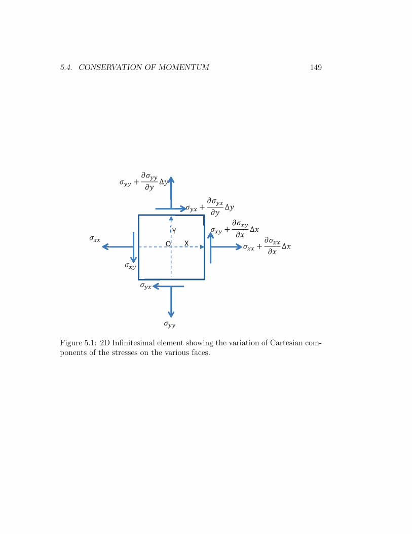
5.4. CONSERVATION OF MOMENTUM 149
O
X
Y
Figure 5.1: 2D Infinitesimal element showing the variation of Cartesian com-ponents of the stresses on the various faces.
150 CHAPTER 5. BALANCE LAWS
force, b with Cartesian components bx and by along the x and y directionrespectively. Also, we shall assume that the infinitesimal element is acceler-ating with acceleration, a with Cartesian components ax and ay along the xand y direction respectively. Thus, force equilibrium along the x directionrequires:
ρ(∆x)(∆y)(1)ax =
[σxx(x, y) +
∂σxx∂x|(x,y)∆x− σxx(x, y)
](∆y)(1)
+
[σyx(x, y) +
∂σyx∂y|(x,y)∆y − σyx(x, y)
](∆x)(1)
+ρ(∆x)(∆y)(1)bx, (5.22)
where ρ is the density and the element is assumed to have a unit thickness.Note that here ρ(∆x)(∆y)(1) gives the infinitesimal mass of the element andthe stresses are multiplied by the respective areas over which they act toget the forces; since only the forces should satisfy the equilibrium equations.Simplifying, (5.22) we obtain:
ρax =∂σxx∂x
+∂σyx∂y
+ ρbx. (5.23)
Similarly, writing the force equilibrium equation along the y direction:
ρ(∆x)(∆y)(1)ay =
[σxy(x, y) +
∂σxy∂x|(x,y)∆x− σxy(x, y)
](∆y)(1)
+
[σyy(x, y) +
∂σyy∂y|(x,y)∆y − σyy(x, y)
](∆x)(1)
+ρ(∆x)(∆y)(1)by. (5.24)
The above equation simplifies to:
ρay =∂σxy∂x
+∂σyy∂y
+ ρby. (5.25)
Finally, we appeal to the moment equilibrium. Here we assume that thereare no body couples or contact couples acting in the infinitesimal element.Since, we can take moment equilibrium about any point, for convenience, wedo it about the point O, marked in figure 5.1, to obtain:[
σxy(x, y) + σxy(x, y) +∂σxy∂x|(x,y)∆x
](∆x)
2(∆y)(1)
=
[σyx(x, y) + σyx(x, y) +
∂σyx∂y|(x,y)∆y
](∆y)
2(∆x)(1).(5.26)

5.4. CONSERVATION OF MOMENTUM 151
Simplifying the above equation we obtain:
σxy +∂σxy∂x
∆x
2= σyx +
∂σyx∂y
∆y
2, (5.27)
which in the limit ∆x and ∆y tending to zero, the limit that we are interestedin, reduces to requiring
σxy = σyx. (5.28)
Thus, a plane Cauchy stress field should satisfy the equations (5.23),(5.25) and (5.28) for it to be admissible.
Generalizing it for 3D, the Cauchy stress field should satisfy:
ρax =∂σxx∂x
+∂σyx∂y
+∂σzx∂z
+ ρbx, (5.29)
ρay =∂σxy∂x
+∂σyy∂y
+∂σzy∂z
+ ρby, (5.30)
ρaz =∂σxz∂x
+∂σyz∂y
+∂σzz∂z
+ ρbz, (5.31)
andσxy = σyx, σxz = σzx, σyz = σzy. (5.32)
The equations (5.29) through (5.31) are written succinctly as
ρa = div(σ) + ρb, (5.33)
and equations (5.32) tells us that the Cauchy stress should be symmetric.Similarly, requiring a sector of cylindrical shell to be in equilibrium, under
the action of spatially varying stresses, it can be shown that
ρar =∂σrr∂r
+1
r
∂σθr∂θ
+∂σzr∂z
+σrr − σθθ
r+ ρbr, (5.34)
ρaθ =∂σrθ∂r
+1
r
∂σθθ∂θ
+∂σzθ∂z
+σrθ + σθr
r+ ρbθ, (5.35)
ρaz =∂σrz∂r
+∂σθz∂θ
+∂σzz∂z
+σrzr
+ ρbz, (5.36)
andσrθ = σθr, σrz = σzr, σθz = σzθ. (5.37)
has to hold.
152 CHAPTER 5. BALANCE LAWS
5.4.1 Conservation of linear momentum
Let At be an arbitrary sub-region in the configuration Bt of a body B. Thetotal linear momentum, Γ(At), of the material particles occupying At is de-fined by
Γ(At) =
∫At
ρvdv. (5.38)
Next, we find the forces acting on the body. Since, the part At hasbeen isolated from its surroundings, traction t(n)(x), introduced in the lastchapter, acts on the boundary of the At. In addition to traction, which arisesbetween parts of the body that are in contact, there exist forces like gravitywhich act on the material particles not through contact and are called bodyforce. The body forces are denoted by b and are defined per unit mass.Hence, the resultant force, z acting on At is
z(At) =
∫∂At
t(n)da+
∫At
ρbdv. (5.39)
Now, using Newton’s second law of motion, which states that the rate ofchange of linear momentum of the body must equal the resultant force thatacts on the body in both magnitude and direction we obtain
DΓ
Dt=
D
Dt
∫At
ρvdv =
∫∂At
t(n)da+
∫At
ρbdv = z. (5.40)
Using (3.30), definition of acceleration, a and (5.16) the above equation canbe written as ∫
At
ρDv
Dtdv =
∫At
ρadv =
∫∂At
t(n)da+
∫At
ρbdv. (5.41)
Next, using Cauchy’s stress theorem (4.3) and the divergence theorem (2.263)the above equation further can be reduced to∫
At
ρadv =
∫∂At
σnda+
∫At
ρbdv =
∫At
[div(σ) + ρb] dv. (5.42)
Since, the above equation has to hold for Bt and any subset, At, of it
ρa = div(σ) + ρb. (5.43)

5.4. CONSERVATION OF MOMENTUM 153
Many a times, we are interested in cases for which a = o, then (5.43)becomes
div(σ) + ρb = o, (5.44)
which is referred to as Cauchy’s equation of equilibrium. Further, there arisesscenarios where the body forces can be neglected and in those cases div(σ) =o. Thus, divergence free stress fields are called self equilibrated stress fields.
Equation (5.43) is in spatial form, that is it assumes that σ = σ(x, t), b =b(x, t), a = a(x, t), ρ = ρ(x, t) are known. But on most occasions, especiallyin solid mechanics, we know only the material form of these fields that is σ= σ(X, t), b = b(X, t), a = a(X, t), ρ = ρ(X, t) and in those occasions itis difficult to obtain the spatial divergence of these fields. To make it easierat these instances, we seek a statement of balance of linear momentum inmaterial form. For this, equation (5.42a) has to be modified. Towards this,we obtain ∫
At
ρadv =
∫Ar
ρa det(F)dV =
∫Ar
ρradV
=
∫∂At
σnda+
∫At
ρbdv
=
∫∂Ar
det(F)σF−tNdA+
∫Ar
ρb det(F)dV
=
∫Ar
Div(P)dV +
∫Ar
ρrbdV, (5.45)
for which we have successively used equation (3.75), (5.14), (3.72) and def-inition of Piola-Kirchhoff stress (4.42) and the divergence theorem. Since,(5.45) has to hold for any arbitrary subpart of the reference configuration,we obtain the material differential form of the balance of linear momentumas
ρra = Div(P) + ρrb. (5.46)
It is worthwhile to emphasize that irrespective of the choice of the in-dependent variable, the equilibrium of the forces is established only in thecurrent configuration. In other words, whether we use material or spatialdescription for the stress, the forces and moments have to be equilibrated inthe deformed configuration and not the reference configuration.

154 CHAPTER 5. BALANCE LAWS
5.4.2 Conservation of angular momentum
Let At be an arbitrary sub-region in the configuration Bt of a body B. Thetotal angular momentum, Ω(At), of the material particles occupying At isdefined by
Ω(At) =
∫At
[(x− xo) ∧ ρv + p]dv, (5.47)
where xo is the point about which the moment is taken and p is the intrinsicangular momentum per unit volume in the current configuration.
Next, we find the moment due to the forces acting on the body. Asdiscussed before there are two kind of forces, surface or contact forces andbody forces act on the body which contribute to the moment. Apart frommoment arising due to applied forces, there could exist couples distributedper unit surface area, m and body couples c, defined per unit mass. Thus,m = m(x, t,n) and c = c(x, t). Hence, the resultant moment, ω acting onAt is
ω(At) =
∫∂At
[(x− xo) ∧ t(n) + m]da+
∫At
[ρ(x− xo) ∧ b + c]dv. (5.48)
However, in non-polar bodies that are the subject matter of the study here,there exist no body couples or couples distributed per unit surface area orintrinsic angular momentum, i.e., c = m = p = o.
The balance of angular momentum states that the rate of change of theangular momentum must equal the applied momentum in both direction andmagnitude. Hence,
DΩ
Dt= ω. (5.49)
Further simplification of this balance principle involves some tensor algebra.First, we begin by calculating the left hand side of the above equation:
DΩ
Dt=
D
Dt
[∫At
[(x− xo) ∧ ρv + p]dv
]=
∫Ar
D
Dt[(x− xo) ∧ ρv + p] det(F) dV
=
∫Ar
v ∧ ρv det(F) + (x− xo) ∧D
Dt(ρ det(F))v + ρa det(F)
dV
+
∫Ar
D
Dt(p det(F)) dV. (5.50)
5.4. CONSERVATION OF MOMENTUM 155
Since, v ∧ v = o and using equations (5.13) and (5.9), (5.50) reduces to
DΩ
Dt=
∫Ar
[(x− xo) ∧ ρa] det(F)dV +
∫Ar
[Dp
Dt+ pdiv(v)
]det(F)dV
=
∫At
[(x− xo) ∧ ρa] +
Dp
Dt+ pdiv(v)
dv. (5.51)
Next, we simplify the right hand side of the equation (5.49). Towardsthat, we first show that∫
∂At
(x− xo) ∧ σtnda =
∫At
[(x− xo) ∧ div(σ)− τ ] dv, (5.52)
where τ is the axial vector of (σ − σt). We begin by establishing a fewvector identities which enable us to establish (5.52).
Identity - 1: If u and v are arbitrary vectors then u ∧ v is the axialvector of the skew-symmetric tensor v ⊗ u − u⊗ v.
Proof: It is straightforward to verify that v ⊗ u − u ⊗ v is skew-symmetric. Then we observe that
(v ⊗ u− u⊗ v)(u ∧ v) = u · (u ∧ v)v − v · (u ∧ v)u = o, (5.53)
hence, the axial vector of v⊗u−u⊗v is a scalar multiple of u∧v. Accordingly,
(v ⊗ u− u⊗ v)a = (a · u)v − (a · v)u = α(u ∧ v) ∧ a, (5.54)
for any vector a. Now, we have to show that α = 1. Setting a = u in theabove equation and then forming a scalar product on each side with v wehave
(u · u)(v · v)− (u · v)2 = α(u ∧ v) ∧ u · v (5.55)
Using (2.36) we find that
α(u ∧ v) ∧ u · v = α[(u · u)(v · v)− (u · v)2]. (5.56)
Comparing equations (5.55) and (5.56) we find that α = 1.Identity - 2: For any vector a, b, c in the vector space
a ∧ (b ∧ c) = (b⊗ c− c⊗ b)a. (5.57)
This identity follows immediately from the above identity.
156 CHAPTER 5. BALANCE LAWS
Identity - 3: Let At be a regular region with boundary ∂At, let n bethe outward unit normal to ∂At and let u be a vector field and σ a tensorfield, each continuous in At and continuously differentiable in the interior ofAt. Then ∫
∂At
u⊗ σnda =
∫At
u⊗ div(σ) + grad(u)σdv. (5.58)
Towards proving this identity, note that∫∂At
(σn⊗ u)ada =
∫∂At
(u · a)σnda =
∫At
div((u · a)σ)dv
=
∫At
[(u · a)div(σ) + σtgrad(u · a)dv
=
∫At
[div(σ)⊗ u + σtgrad(u)t]adv (5.59)
where a is an arbitrary constant vector. To obtain the above we have madeuse of the identities∫
∂v
Tnda =
∫v
div(T)dv, (5.60)
div(ΦT) = Φdiv(T) + Ttgrad(Φ), (5.61)
and the definition of the gradient. Further, since a is arbitrary in (5.59) wehave the identity∫
∂At
σn⊗ uda =
∫At
[div(σ)⊗ u + σtgrad(u)t]dv (5.62)
Taking the transpose of the above identity, we obtain the required vectoridentity (5.58).
Now, we are in a position to prove (5.52). For this we replace b by (x−xo)and c by σn in (5.57) and then integrating each side over the surface ∂At weobtain
a∧∫∂At
(x−xo)∧(σn)da =
(∫∂At
(x− xo)⊗ (σn)− (σn)⊗ (x− xo)da)
a,
(5.63)
5.4. CONSERVATION OF MOMENTUM 157
a being an arbitrary vector. From (5.58) it follows that∫∂At
(x− xo)⊗ (σn)da =
∫At
(x− xo)⊗ div(σ) + σdv, (5.64)∫∂At
(σn)⊗ (x− xo)da =
∫At
div(σ)⊗ (x− xo) + σtdv, (5.65)
Substituting the above equations in (5.63), we obtain
a ∧∫∂At
(x− xo) ∧ (σn)da =
∫At
[(x− xo)⊗ div(σ)− div(σ)⊗ (x− xo)]a
+(σ − σt)adv (5.66)
Again using (5.57) and the definition of axial vector to a skew-symmetrictensor (2.98) the above equations can be reduced to
a ∧∫∂At
(x− xo) ∧ (σn)da = a ∧∫At
[(x− xo) ∧ div(σ)− τ ]dv, (5.67)
and hence the required identity (5.52), since a is an arbitrary vector.Substituting (5.51) and (5.52) in (5.49) yields∫
∂At
mda =
∫At
[(x− xo) ∧ (ρa− div(σ)− ρb)]dv
+
∫At
[Dp
Dt+ pdiv(v)− c + τ ]dv. (5.68)
Since, the body also satisfies the balance of linear momentum (5.43), the firstterm on the RHS is zero. Hence, the balance of angular momentum requires∫
∂At
mda =
∫At
[Dp
Dt+ pdiv(v)− c + τ ]dv. (5.69)
Here we are interested only in non-polar bodies and hence, p = c = m = o.Therefore, (5.69) simplifies to requiring∫
At
τdv = o. (5.70)
Since, this has to hold for any arbitrary subparts of the body, Bt, τ = o.Consequently,
σ = σt, (5.71)
that is the Cauchy stress tensor has to be symmetric in non-polar bodies.

158 CHAPTER 5. BALANCE LAWS
5.5 Summary
Since, in this course we are interested only in purely mechanical process, westudied only conservation of mass and momentum. There are other quantitieslike energy, charge which is also conserved. In courses on thermodynamicsor electromagnetism, one would study the other conservation laws. The oneequation that would be used frequently in the following chapters is the finalexpression for the conservation of linear momentum, also called as equilib-rium equations,
ρa = div(σ) + ρb, (5.72)
where ρ is the density, b is the body force per unit mass, σ is the Cauchystress tensor.
5.6 Self-Evaluation
1. Determine which of the following Cauchy stress fields are possible withina body at rest assuming that there are no body forces acting on it:
(a) σ =
−32x2y2 xy3 0xy3 −1
4y4 0
0 0 0
,
(b) σ =
3yz z2 5y2
z2 7xz 2x2
5y2 2x2 9xy
,
(c) σ =
3x+ 5y 7x− 3y 07x− 3y 2x− 7y 0
0 0 0
,
(d) σ =
3x −3y 0−7x 7y 0
0 0 0
,
(e) σ =
7x −3x 07y 3y 00 0 0
,
where the components of the stress are with respect to orthonormalCartesian basis and (x, y, z) denote the Cartesian coordinates of a typ-ical material particle in the current configuration of the body.
5.6. SELF-EVALUATION 159
2. The Cartesian components of the Cauchy stress tensor in a plate atrest is
σ =
−2x2 −7 + 4xy + z 1 + x− 3y−7 + 4xy + z 3x2 − 2y2 + 5z 0
1 + x− 3y 0 −5 + x+ 3y + 3z
.
Find the body force that should act on the plate so that this state ofstress is realizable in the body.
3. A body at rest is subjected to a plane state of stress such that thenon-zero Cartesian components of the Cauchy stress are σxx, σxz andσzz. Derive the equilibrium equations for this special case. Then, showthat in the absence of body forces the equilibrium equations hold if,
σxx =∂2φ
∂z2, σxz = − ∂2φ
∂x∂z, σzz =
∂2φ
∂x2,
where φ = φ(x, y), for any choice of φ. φ is called the Airy’s stresspotential.
4. Derive form first principles and show that for the plane stress prob-lem in cylindrical polar coordinates with the non-zero cylindrical polarcomponents of the Cauchy stress being σrr, σrθ and σθθ, as shown infigure 5.2, the equilibrium equations in the absence of body forces withthe body in static equilibrium are
∂σrr∂r
+1
r
∂σθr∂θ
+σrr − σθθ
r= 0,
∂σrθ∂r
+1
r
∂σθθ∂θ
+2σrθr
= 0.
5. Is any stress field that satisfies the equilibrium equations realizable ina given body? Discuss.

160 CHAPTER 5. BALANCE LAWS
dz
r dθ
dr
Figure 5.2: Figure for problem 4. Variation of the cylindrical polar compo-nents of the Cauchy stress over an infinitesimal cylindrical wedge, in planestress state

Chapter 6
Constitutive Relations
6.1 Overview
The concepts and equations introduced in chapters 3 to 5, within the frame-work of non-relativistic mechanics, are essential to characterize kinematics,stresses and balance principles and as mentioned already these concepts andequations hold for any body undergoing a purely mechanical process. How-ever, they do not distinguish one material from another which is contra-dictory with the experiments. Also, for a non-polar body while there areonly seven equations1 there are thirteen2 scalar fields that needs to be deter-mined. Thus, there are more unknowns in the balance laws than availableequations and hence all of the unknown fields cannot be determined fromthe balance laws alone. In other words, balance laws alone are incapable ofdetermining the response (displacement of the body due to an applied force)of deformable bodies3. They must be augmented by additional equations,called constitutive relations or equations of state, which depends on the ma-terial that the body is made up of. A constitutive relation approximates theobserved physical behavior of a material under specific conditions of interest.To summarize, constitutive relations are required for two reasons:
• To bring in the material dependence in the force displacement relation.
1As we saw in the last chapter, there are 1 equation due to balance of mass, 3 equationsdue to balance of linear momentum and 3 equations due to balance of angular momentum.
2The thirteen scalar fields are: density, three components for body force and ninecomponents of stress. Here we assume that the body is non-polar.
3If we were to specify a body as rigid, then balance laws alone is sufficient to determineits motion. However, specifying a body as rigid is a constitutive specification.
161
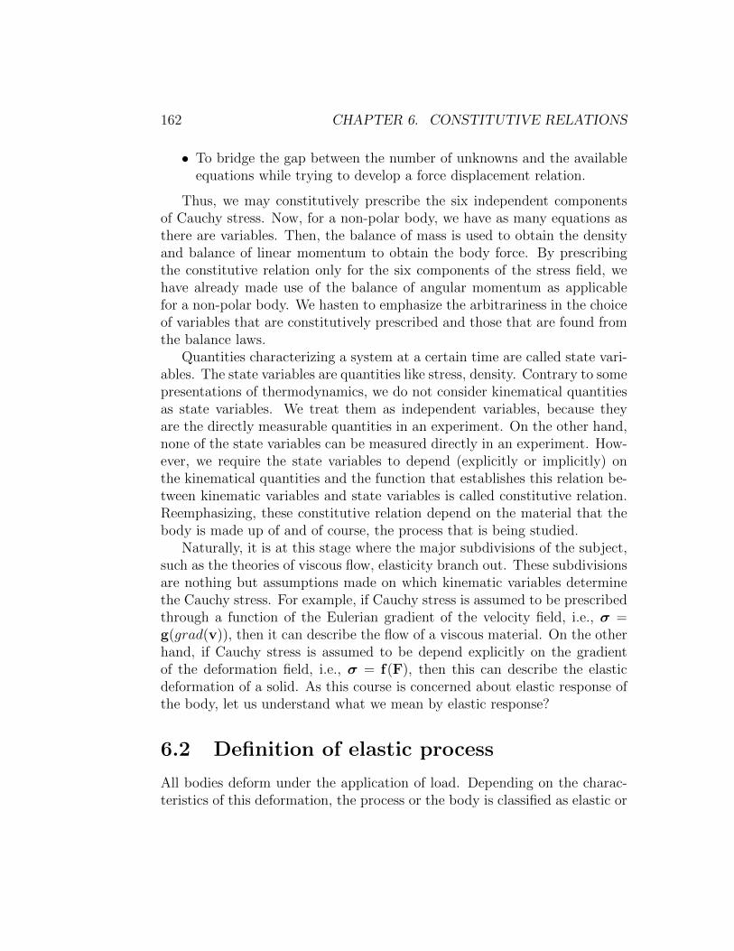
162 CHAPTER 6. CONSTITUTIVE RELATIONS
• To bridge the gap between the number of unknowns and the availableequations while trying to develop a force displacement relation.
Thus, we may constitutively prescribe the six independent componentsof Cauchy stress. Now, for a non-polar body, we have as many equations asthere are variables. Then, the balance of mass is used to obtain the densityand balance of linear momentum to obtain the body force. By prescribingthe constitutive relation only for the six components of the stress field, wehave already made use of the balance of angular momentum as applicablefor a non-polar body. We hasten to emphasize the arbitrariness in the choiceof variables that are constitutively prescribed and those that are found fromthe balance laws.
Quantities characterizing a system at a certain time are called state vari-ables. The state variables are quantities like stress, density. Contrary to somepresentations of thermodynamics, we do not consider kinematical quantitiesas state variables. We treat them as independent variables, because theyare the directly measurable quantities in an experiment. On the other hand,none of the state variables can be measured directly in an experiment. How-ever, we require the state variables to depend (explicitly or implicitly) onthe kinematical quantities and the function that establishes this relation be-tween kinematic variables and state variables is called constitutive relation.Reemphasizing, these constitutive relation depend on the material that thebody is made up of and of course, the process that is being studied.
Naturally, it is at this stage where the major subdivisions of the subject,such as the theories of viscous flow, elasticity branch out. These subdivisionsare nothing but assumptions made on which kinematic variables determinethe Cauchy stress. For example, if Cauchy stress is assumed to be prescribedthrough a function of the Eulerian gradient of the velocity field, i.e., σ =g(grad(v)), then it can describe the flow of a viscous material. On the otherhand, if Cauchy stress is assumed to be depend explicitly on the gradientof the deformation field, i.e., σ = f(F), then this can describe the elasticdeformation of a solid. As this course is concerned about elastic response ofthe body, let us understand what we mean by elastic response?
6.2 Definition of elastic process
All bodies deform under the application of load. Depending on the charac-teristics of this deformation, the process or the body is classified as elastic or

6.2. DEFINITION OF ELASTIC PROCESS 163
inelastic. The characteristics of this deformation depends on the material,temperature, magnitude of the applied load and among many other factors.Now, let us understand the characteristics of a elastic process.
Some of the definitions of an elastic process in the literature are:
1. The processes in which the original size and shape can be recovered istermed as elasticity.
2. Processes in which, the value of state variables in a given configurationare independent of how it was reached is called elastic.
3. A non-dissipative process is called a elastic process.
The first two definitions are popular in the literature. However, they areof little use because they cannot tell whether a process that the body iscurrently being subjected to is elastic. Such a conclusion can be arrived atonly after subjecting the body to a complementary process. However, thelast definition does not have such a drawback.
Further, it turns out that these various definitions are not equivalent. Tosee this, consider the uniaxial stress versus stretch ratio plot shown in figure6.1a. Such a response, possible in shape memory alloys, would qualify aselastic only if the first definition is used. Since, the stress corresponding toa given stretch ratio depends on whether it is being loaded or unloaded itis not elastic according to the second definition. Also, since the loading andunloading path are different, there will be dissipation (wherein the mechan-ical energy is converted into thermal energy). Hence, it cannot be elastic bythe last definition either.
Consider a axial stress vs. stretch response as shown in figure 6.1b whichwill be characterized as elastic according to definitions one and three. Butthe value of state variable stress could be anything corresponding to a stretchratio of Λo. Hence, it is not elastic according to definition two. Of course,such a stress versus stretch response occurs for an idealized system made of aspring and an inextensible chord as shown in figure 6.1c. But then elasticityis an idealized process too and biological soft tissues response can be idealizedas shown in figure 6.1b.
For us, a process is elastic only if it is consistent with all three definitions.
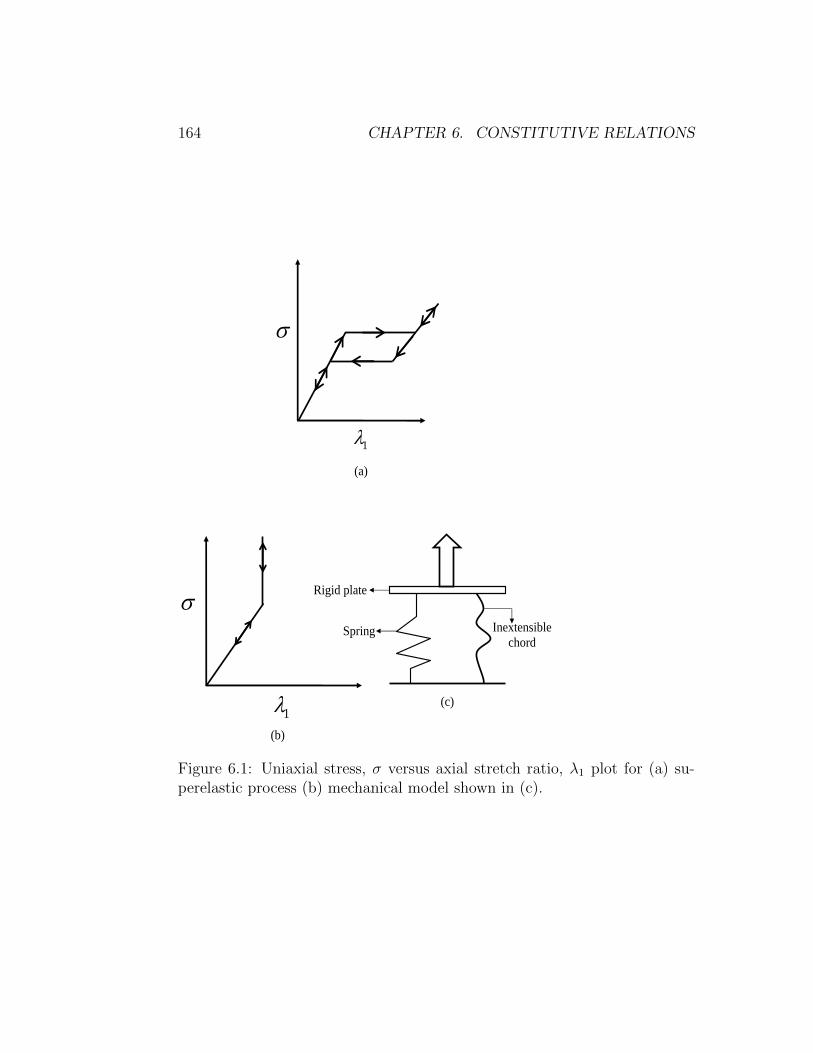
164 CHAPTER 6. CONSTITUTIVE RELATIONS
1
(a)
1(b)
Rigid plate
Spring Inextensiblechord
(c)
Figure 6.1: Uniaxial stress, σ versus axial stretch ratio, λ1 plot for (a) su-perelastic process (b) mechanical model shown in (c).

6.2. DEFINITION OF ELASTIC PROCESS 165
Before proceeding further a few words of caution is necessary. In reality,no process is elastic but some are close to being elastic. It is common in theliterature, as we also did in the first paragraph, to call a material or a bodyto be elastic. This is incorrect, in a strict sense. It is the process that thebody is being subjected to which is elastic. After all, the same body underdifferent circumstances deforms inelastically.
Based on the above definition of elasticity, it can be shown that theCauchy stress, σ, in an elastic process would at most depend on the defor-mation gradient, F, three material unit vectors, Mi and the state of Cauchystress in the reference configuration4, σR and thus,
g(σ,F,σR,M1,M2,M3) = 0. (6.1)
In other words, equation (6.1) is an assumption on how the state variable,stress, varies with the motion of the body. Since, by definition 2 for anelastic process, the value of stress cannot depend on the history of the motionfield that the body has experienced, we are assured that there is an implicitfunction that relates the Cauchy stress and the deformation gradient.
We shall assume σR = 0, that is the reference configuration is stress freeand that the Cauchy stress is related explicitly to the deformation gradient,so that equation (6.1) could be simplified to,
σ = h(F,M1,M2,M3). (6.2)
Further if we assume that the material is isotropic, that is the response ofthe material is same in all directions (see section 6.3.2 for more detaileddiscussion), the Cauchy stress would not depend on the three unit materialvectors, Mi. For this case, the Cauchy stress depends explicitly only on thedeformation gradient, i.e.,
σ = f(F). (6.3)
Thus, we have to find the relation between the six independent com-ponents of the stress tensor and the nine independent components of thedeformation gradient. To find this relation in general through experimenta-tion alone is daunting, as we illustrate now. Let us say the relation betweenthe components of the Cauchy stress (σij) and deformation gradient (Fkl) islinear and of the form,
σij = Cijkl(Fkl − δkl), (6.4)
4Do not confuse the stress in the reference configuration with Piola-Kirchhoff stresses.While σR = f(1,σR), Piola-Kirchhoff stress, P = det(F)f(F,σR)F−t.
166 CHAPTER 6. CONSTITUTIVE RELATIONS
where Cijkl is the components of a constant fourth order tensor and δkl isthe Kronecher delta. Even for this case, we have to find 6*9 = 54 constantswhich means we require 54 independent measurements. This is too many.While for metals this relationship is linear for polymers it is nonlinear. Itis easy to see that the number of constants required in case of nonlinearrelationship would be much higher than the linear case. Hence, if there issome way by which we can reduce the number of unknown functions from6 and the variables that it depends on from 9 in equation (6.3) it would beuseful. It turns out that this is possible and this is what we shall see next.
6.3 Restrictions on constitutive relation
There are certain restrictions, guidelines and principles that are commonwhich the constitutive relations for different materials and under differentconditions of interest, should satisfy. Thus, we require the constitutive rela-tion to ensure that the value of the state variables for a given state of thebody are independent of the placement of the body in the Euclidean spaceand to honor the coordinate transformation rules. There is also, the conceptof material symmetry which to a large extent determines the variables in theconstitutive relation. The following section is devoted towards understandingthese concepts.
6.3.1 Restrictions due to objectivity
While the physical body was given a mathematical representation, we madetwo arbitrary choices regarding:
1. The region in the Euclidean point space to which the body is mapped.
2. The orientation of the basis vectors with respect to which the position,velocity, acceleration, etc. of the material particles are defined.
Since these choices are arbitrary, the state of the body cannot depend onthese choices. (Clearly, a body subjected to a particular load cannot failjust because, the body is mapped on to a different region of Euclidean pointspace or a different set of basis vectors is used.) Hence, the constitutiverelations that relate these state variables with the independent variables,i.e., kinematic variables, should also not depend to these choices.

6.3. RESTRICTIONS ON CONSTITUTIVE RELATION 167
The value of state variables variables have to be invariant with respect tothe above choices because they mathematically describe the state of the body.We emphasize that the value of the state variables have to be invariant andnot same. Thus, while the value of scalar valued state variables like densityhave to be the same, the components of tensor valued state variables likestress will change with the choice of the basis according to the transformationrules discussed in section 2.6. However, as pointed out in 2.6 just because thecomponents of a tensor is different does not mean they are different tensors.Only, if the value of at least one of the certain scalar valued functions ofthe components of the tensor are different5, the two tensors are said to bedifferent.
Restriction due to non-uniqueness of placers
In this section, we shall explore the restrictions that needs to be placedon the constitutive relations so that they remain invariant for the differentequivalent mappings of the body on to the Euclidean point space. From aphysical standpoint, the same restriction could be viewed as requiring theconstitutive relation of the body be the same irrespective of where the bodyis. That is, say, the deflection of the beam to a given set of loads shouldremain the same whether it is tested in Chennai or Delhi or Washington orLondon.
It should be realized that in the different mappings of the body ontothe Euclidean space, it is the point space that changes and not the vectorspace. If the vector space were to change, it means that we are changing thebasis vectors. Further, it is assumed that the scale used to measure distancesbetween two points does not change. Consequently, the distance betweenany two points in the body does not change due to these different mappingsof the body. Hence, this restriction, as we shall see, tantamount to requiringthat the state variables be invariant to superposed rigid body rotation of thecurrent or the reference configuration.
Let x and x+ denote the position vector of a material particle at time t,mapped on to different regions of the Euclidean point space. Then, they are
5For example, if A is a second order tensor then one of the following: tr(A), tr(A−1),det(A), must be different. There is nothing unique about the choice of the scalar valuedfunctions of A. One could have chosen tr(A2) instead of det(A) or more generally, tr(Am)where m takes some integer value.
168 CHAPTER 6. CONSTITUTIVE RELATIONS
related by the equation:x+ = Qx + c, (6.5)
where Q and c are functions of time, t and Q is an orthogonal tensor, notnecessarily a proper orthogonal tensor6. While it is easy to see that (6.5)preserves the distance between any two points, the converse can be provedby following the same steps as that outlined in section 3.10.1.
Since, similar non-uniqueness exist with respect to placers for the refer-ence configuration
X+ = QoX + co, (6.6)
where X and X+ are the position vectors of same material particle mappedon to the different regions of the Euclidean point space, Qo is a constantorthogonal tensor and co is a constant vector.
Next, we like to compute the standard kinematical quantities and seehow they change due to these equivalent mappings of the body on to theEuclidean point space. This is a prerequisite to find the restrictions on theconstitutive relations due to this requirement.
We begin by considering the transformations of the motion field, χ. Let
x = χ(X, t), x+ = χ+(X+, t) (6.7)
then using equations (6.5) and (6.6) we obtain
x+ = χ+(X+, t) = Qχ(X, t) + c = Qχ(Qto(X
+ − co), t) + c, (6.8)
Now, we can find the relation between the deformation gradients, F andF+ defined as
F =∂x
∂X, F+ =
∂x+
∂X+, (6.9)
using (6.6), (6.8) and chain rule for differentiation to be
F+ = QF∂X
∂X+= QFQt
o. (6.10)
Next, we find the relation between the velocity fields, v and v+ definedas
v =Dx
Dt, v+ =
Dx+
Dt, (6.11)
6We allow improper orthogonal tensors because what is considered as top or bottom,left or right is subjective.

6.3. RESTRICTIONS ON CONSTITUTIVE RELATION 169
using equation (6.5) as
v+ = Qv +DQ
Dtx +
Dc
Dt= Qv +
DQ
DtQt(x+ − c) +
Dc
Dt. (6.12)
Similarly, we obtain the relationship between accelerations a and a+ as
a+ = Qa + 2DQ
Dtv +
D2Q
Dt2x +
D2c
Dt2. (6.13)
In order to simplify equations (6.12) and (6.13) we introduce, the skew tensor
Ω =DQ
DtQt. (6.14)
To show that Ω is a skew tensor, taking the total time derivative of therelation QQt = 1, we obtain
DQ
DtQt + Q
DQt
Dt= 0, (6.15)
from which the required result follows. In lieu of definition (6.14), equations(6.12) and (6.13) can be written as
v+ = Qv +Dc
Dt+ Ω(x+ − c), (6.16)
a+ = Qa +D2c
Dt2+ 2Ω
(v+ − Dc
Dt
)+
(DΩ
Dt−Ω2
)(x+ − c).(6.17)
where we have made use of the identity
DQ
Dtv = Ω
(v+ − Dc
Dt
)−Ω2(x+ − c),
to obtain (6.17).
Now, we would like to see how the displacement transforms due to differ-ent placements of the body in the Euclidean point space. Recalling that thedisplacement field is defined as:
u = x−X, u+ = x+ −X+. (6.18)

170 CHAPTER 6. CONSTITUTIVE RELATIONS
The Eulerian displacement gradient transforms like
h =∂u
∂x= 1− F−1,
h+ =∂u+
∂x+= 1− (F+)−1
= 1−QoF−1Qt = 1−QoQ
t + QohQt, (6.19)
where we have used (6.10) and (3.34). Similarly, the Lagrangian displacementgradient, is computed to be
H =∂u
∂X= F− 1,
H+ =∂u+
∂X+= F+ − 1 = QHQt
o + QQto − 1, (6.20)
using (6.10) and (3.33). It is apparent from the above equations that dis-placement gradient transforms as QhQt (or QoHQt
o) only if Q = Qo.Then, it is straightforward to show that the right and left Cauchy-Green
deformation tensor transform as:
C+ = QoCQto, B+ = QBQt. (6.21)
Next, we examine what happens to stress tensors due to different placementsof the body in the current configuration. Recalling traction is related to theCauchy stress, by the relation t(n) = σn, where n is the outward unit normalat a point x on the boundary surface ∂Bt of an arbitrary region Bt.
As evidenced from the figure (6.2) a different placer of the body in theEuclidean space, in general, alters the orientation of the normal with respectto a fixed set of basis vectors. Let n and n+ denote the outward unit normalsto the same material surface ∂B and at the same material particle, P , in twodifferent placements of the body in the Euclidean space, Bt and B+
t . Since,we are interested in the same material surface, we can appeal to Nanson’sformula (3.72) to relate the unit normals as
n+ = Qn. (6.22)
where we have made use of the equation (6.5) which provides the relationshipbetween the placements Bt and B+
t .

6.3. RESTRICTIONS ON CONSTITUTIVE RELATION 171
n
t(n)
1
nt(n)
2
Figure 6.2: Two placements (κ1, κ2) of the same body in the same statealong with a unit normal (n) and traction (t(n)).
Similarly, the traction vector t(n) and t+(n+) acting on the same material
surface, ∂B and at the same material particle P , in two different placementsof the body, Bt and B+
t are related through:
t+(n+) = Qt(n). (6.23)
To obtain the above equation we have made use of the fact that the normaland shear traction acting on a material surface in two different placementsof the body in the current configuration has to be same, i.e., t+
(n+) · n+ =
t(n) · n. Then, (6.23) is obtained by recognizing that (Qtt+(n+) − t(n)) · n = 0
for any choice of n where we have made use of (6.22).Since, t+
(n+) = σ+n+ and t(n) = σn, we obtain
Qσn = σ+Qn, (6.24)
using equations (6.22) and (6.23) and the above equation has to hold for anychoice of n. Therefore, the Cauchy stress will transform as
σ+ = QσQt. (6.25)
Since, the definition of Cauchy stress is independent of the choice of referenceconfiguration, different placers of the reference configuration, does not causeany change in the value of the Cauchy stress.
172 CHAPTER 6. CONSTITUTIVE RELATIONS
Next, let us see how body forces transform. These forces are essentiallyaction at a distance forces acting along a straight line joining the materialparticles in the body under investigation to another point in space belongingto some other body. Thus, if r is the position vector of the point belongingto another body, then the direction along which b acts, is given by (x−r)/(|x−r |). Then, in a different placement of the body the body force acts alonga direction (x+ − r+)/(| x+ − r+ |). Because the new placement of the bodyis related to its original placement by equation (6.5), we obtain
b+ = b(| x+ − r+ |) x+ − r+
| x+ − r+ |= b(| Qx−Qr |) Qx−Qr
| Qx−Qr |
= b(| x− r |)Q(x− r)
| x− r |= Qb, (6.26)
where b(·) denotes a function of the distance between two points of interest.Here r+ = Qr + c because the transformation rule is applicable not onlyto points that the body under study occupies but to its neighboring bodiesas well. This is required so that the relationship between the body underinvestigation and its neighbors are preserved.
Finally, for future reference, div(σ) transforms due to equivalent place-ments of the body as,
div+(σ+) = div(σ+)Q = div(QσQt)Q = Qdiv(σ), (6.27)
where div+ denotes the divergence with respect to x+.Till now, we have just seen how various quantities transform between
different placements of the same body in the same state. Using this we arein a position to state what restriction the requirement that the state variablesbe invariant to the different placers of the body in the same state places onthe constitutive relation, given it depends on certain kinematic quantitiesand other state variables. For example, as we saw above for elastic processthe stress is a function of deformation gradient, i.e.,
σ = f(F). (6.28)
Now, due to different placement of the body in the reference and currentconfigurations,
σ+ = f(F+). (6.29)

6.3. RESTRICTIONS ON CONSTITUTIVE RELATION 173
Note that the function does not change and this is what restricts the natureof the function. Using equations (6.25) and (6.10), (6.29) can be written as
σ+ = QσQt = f(F+) = f(QFQto). (6.30)
Substituting for σ from equation (6.28) we obtain a restriction of the formof the function f as:
Qf(F)Qt = f(QFQto), (6.31)
for any orthogonal tensors Q and Qo and F ∈ D ⊆ Lin+, the set of all lineartransformations whose determinant is positive.
The question on how to obtain the form of the function, given the restric-tion (6.31), is dealt in detail next. To understand how this restriction (6.31)fixes the form of the tensor-valued tensor function, let us look at a similarrequirement on scalar-valued scalar function, g(x). Say the restriction on thisscalar function is: g(m ∗ x) = m ∗ g(x), where m is some arbitrary constant.It then immediately tells that the function is a linear function, i.e., g(x) =a ∗ x, where a is some constant. Similarly, it transpires that the restriction(6.31) requires,
σ = f(F) = α01 + α1B + α2B−1, (6.32)
where αi = αi(J1, J2, J3),
J1 = tr(B), J2 = tr(B−1), J3 = [det(B)]1/2 = det(F), (6.33)
are the invariants of B.Now, we show how equation (6.32) is obtained from the restriction (6.31).
Towards this, first we set Q = 1 to obtain,
f(F) = f(FQto) = f(VR) = f(VRQt
o), (6.34)
where we have made use of the polar decomposition theorem (2.116). Then,let us pick Qo = R, since R is also an orthogonal tensor. With this choiceequation (6.34) yields
f(F) = f(V) = f(B). (6.35)
The last equality arises because B = V2 and square-root theorem, (2.147)ensures the existence of an unique V such that V =
√B. Next, we shall
again appeal to equation (6.31) but now we shall not set Q to be 1 to obtain
Qf(B)Qt = f(QBQt), (6.36)
174 CHAPTER 6. CONSTITUTIVE RELATIONS
∀ Q ∈ O. The above equation can be rewritten as
f(B) = Qtf(QBQt)Q, (6.37)
∀ Q ∈ O.Theorem 7.1: A symmetric second order tensor valued function f de-
fined over the space of symmetric second order tensors, satisfies (6.37) if andonly if it has a representation
σ = f(B) = α01 + α1B + α2B2 (6.38)
where α0, α1, α2 are functions of principal invariants of B, Ii, i.e.,
αi = αi(I1, I2, I3). (6.39)
Proof: 7 Before proving the above theorem we prove the following theo-rem:
Theorem 7.2: Let α be a scalar function defined over the space ofsymmetric positive definite second order tensors. Then α(QBQt) = α(B) ∀Q ∈ O if and only if there exist a function α, defined on R+×R+×R+, suchthat α(B) = α(λ1, λ2, λ3), where α(λ1, λ2, λ3) is insensitive to permutationsof λi and λ1, λ2, λ3 are the eigenvalues of B. Hence, α(B) = α(I1, I2, I3).
Proof: 8 Writing B in the spectral form
B = λ1b1 ⊗ b1 + λ2b2 ⊗ b2 + λ3b3 ⊗ b3, (6.40)
where bi’s are the ortho-normal eigenvectors of B and hence
QBQt = λ1Qb1 ⊗Qb1 + λ2Qb2 ⊗Qb2 + λ3Qb3 ⊗Qb3. (6.41)
Since, α(QBQt) = α(B) ∀ Q ∈ O, α(B) must be independent of the orien-tation of the principal directions of B and must depend on B only throughits eigenvalues, λ1, λ2, λ3.
Next, choose Q to be a rotation of π/2 about b3 so that Qb1 = b2, Qb2
= −b1 and Qb3 = b3. Hence,
α(B) = α(λ2b1 ⊗ b1 + λ1b2 ⊗ b2 + λ3b3 ⊗ b3) (6.42)
7Adapted from Serrin [5] and Ogden [6]. The original proof is due to Rivlin and Ericksen[7]
8Adapted from Ogden [6]

6.3. RESTRICTIONS ON CONSTITUTIVE RELATION 175
from which we deduce that α(λ1, λ2, λ3) = α(λ2, λ1, λ3). In similar fashion itcan be shown that α is insensitive to other permutations of λi’s.
Finally, recalling that the eigenvalues are the solutions of the character-istic equation
λ3 − I1λ2 + I2λ− I3 = 0, (6.43)
in principal, λi’s can be expressed uniquely in terms of the principal invariantsand hence α(B) = α(I1, I2, I3).
The converse of the theorem 7.2 is proved easily from the property oftrace and determinants. Hence, we have proved theorem 7.2.
Theorem 7.3: If f satisfies (6.37) then the eigenvalues of f(B) are func-tions of the principal invariants of B.
Proof: Let γ(B) be the eigenvalue of f(B). Then,
det[f(B)− γ(B)1] = 0. (6.44)
The corresponding eigenvalue of f(QBQt) is γ(QBQt) and hence
det[f(QBQt)− γ(QBQt)1] = 0. (6.45)
This can be written as
det[Qf(B)− γ(QBQt)1Qt] = 0, (6.46)
by using (6.37) and the relation QQt = 1. Using the property of determinantsthe above equation reduces to
det[f(B)− γ(QBQt)1] = 0, (6.47)
which has to hold for all Q ∈ O. Comparing (6.44) and (6.47)
γ(QBQt) = γ(B), (6.48)
for all Q ∈ O, which by theorem 2.2 implies that γ(B) = α(I1, I2, I3)Theorem 7.4: If σ = f(B) satisfies (6.37) then f(B) is coaxial with B,
i.e., the principal directions of B and f(B) would be the same.Proof: Consider an eigenvector b1 of B and define an orthogonal trans-
formation Q by
Qb1 = −b1, Qbj = bj if b1 · bj = 0, (6.49)
176 CHAPTER 6. CONSTITUTIVE RELATIONS
i.e. Q is a reflection on the plane normal to b1. Now, QBQt = B and hence,by (6.37), Qσ = σQ. We therefore have
Q(σb1) = σ(Qb1) = −σb1, (6.50)
and we see that Q transforms the vector σb1 into its opposite. Since, theonly vectors transformed by the reflection Q into their opposites are themultiples of b1, it follows that b1 is an eigenvector of σ. Similarly, it can beshown that every eigenvector of B is also an eigenvector of σ. Hence, f(B)is coaxial with B.
Now we prove theorem 7.1.Clearly, if (6.38) along with (6.39) holds then (6.37) is satisfied and hence
we have to prove only the converse.It follows from theorem 7.3 and theorem 7.4 that f(B) is coaxial with B
and its eigenvalues are functions of the principal invariants of B. Let λ1,λ2,λ3
and f1,f2,f3 be the eigenvalues of B and f(B) respectively and consider theequations
α0 + α1λi + α2λ2i = fi, (i = 1, 2, 3) (6.51)
for the three unknowns α0, α1, α2. Assuming the λi and fi are given and thatλi’s are distinct it follows that αi’s are determined uniquely in terms of λiand fi which are themselves determined uniquely by the principal invariantsof B. Thus, since B is coaxial with f(B) and αi are functions of the principalinvariants of B; equation (6.38) follows from (6.51) provided the eigenvaluesof B are distinct, of course. When the eigenvalues of B are not distinct α2
or α1 and α2 could be chosen arbitrarily, depending on whether the algebraicmultiplicity of the eigenvalues is 2 or 3 respectively. However, this choice maycause some αi to become discontinuous even when f(B) remains continuous,Truesdell and Noll [8] and Serrin [5] provide example of such cases.
Finally, from Cayley-Hamilton theorem, (2.142) we obtain
B2 = I1B− I21 + I3B−1. (6.52)
Then, observing that the principal invariants of the positive definite, B, arerelated bijectively to the invariants J1, J2 and J3, as defined in (6.33), wenote that
αi = αi(I1, I2, I3) = αi(J1, J2, J3) (6.53)
for i = (0, 1, 2). Substituting (6.52) and (6.53) in (6.38) we obtain
σ = α01 + α1B + α2B−1. (6.54)
6.3. RESTRICTIONS ON CONSTITUTIVE RELATION 177
Before concluding this section let us investigate a couple of issues. Thefirst issue is whether the balance laws should also be invariant to differentplacements of the body in the same state. A straight forward calculation willshow that balance of mass is invariant to different placements of the samebody in the same state. However, balance of linear momentum and henceangular momentum are not. In fact, due to equivalent placements of thebody, the balance of linear momentum equation transforms as
Qdiv(σ) + ρQb = ρ
(Qa + 2
DQ
Dtv +
D2Q
Dt2x +
D2c
Dt2
). (6.55)
But for the above equation to be consistent, it is required that
2DQ
Dtv +
D2Q
Dt2x +
D2c
Dt2= o, (6.56)
since, div(σ) + ρb = ρa. The above equation holds only for placements forwhich D2c
Dt2= o and Q(t) = Qc, a constant. Thus, a school of thought requires
the constitutive relations describing the state variables to be invariant onlyfor placements of the body related as:
x+ = Qcx + ctt+ co, (6.57)
where Qc is a constant orthogonal tensor, ct and co are constant vectors.Equation (6.57) is called Galilean transformation.
The other school of thought, argues that equivalent placements of thebody in a particular state is a thought experiment to obtain some restrictionon the constitutive relations describing the state variables which is not ap-plicable for balance laws. The rational behind their argument is that for agiven body force, the balance laws will hold only for certain motions of thebody9. On the other hand, there are no such restrictions for the constitutiverelations. Hence, there is no inconsistency if motions that are not admissibleaccording to the balance law are used to find restrictions on the constitutiverelations. We find merit in this school of thought.
The second issue is on the existence of unique placer for the reference con-figuration. Some researchers are of the opinion that the placer to the reference
9As we shall see, within the realms of finite elasticity, Ericksen [9] has showed that inthe absence of body forces, deformations of the form: r = r(R), θ = Θ, z = Z, where(R,Θ, Z) and (r, θ, z) are the coordinates of a material particle in the reference and currentconfiguration respectively, is not possible in some compressible materials.

178 CHAPTER 6. CONSTITUTIVE RELATIONS
configuration has to be unique for agreement on the material symmetry ofthe body. In section 6.3.2, we show that the opinion of these researchers isincorrect.
Restrictions due to non-uniqueness of the basis vectors
We have been writing equations in direct form, that is independent of thechoice of basis vectors. To beginners it is natural to ask the question, ifwe were to continue to write equations in direct form what restriction canthis choice of basis vectors place? To answer this question let us look at anexample. Say, some person investigating the response of some body subjectedto some process finds that Cauchy stress, σ is related to the deformationgradient, F, as σ = α(F− 1), where α is a constant. Even though we havewritten in direct notation, say, we change the basis vectors used to describethe reference configuration, then the matrix components of the Cauchy stresswill not change. However, the matrix components of the deformation gradientwill change resulting in a contradiction and inadmissability of the proposedrelation.
To elaborate, recall that σ = σijei ⊗ ej and F = Fijei ⊗ Ej, whereei is the basis vectors used to represent the current configuration and Ej
is the basis vectors used in the reference configuration. Then, let [σ] and[F] represent the matrix components of the Cauchy stress and deformationgradient with respect to the Ei basis. Similarly, let [σ] and [F] denotethe matrix components of the Cauchy stress and deformation gradient withrespect to the Ei basis. It follows from the transformation laws 2.6 that
[σ] = [σ], [F] = [F][Q], (6.58)
where Qij = Ei · Ej. Immediately, the contradiction in the constitutiverelation, σ = α(F− 1) is apparent.
Let us see what restriction is placed on the form of the function (orfunctional) to ensure that it obeys the necessary transformation rules. Thus,say, we postulate that: σ = f(F). Let Qij = ei · ej and Qo
ij = Ei · Ej. Dueto this transformation of the basis vectors in the current and the referenceconfiguration, the stress transforms as [σ] = [Q]t[σ][Q] and the deformationgradient transforms as [F] = [Q]t[F][Qo]. Then, we require that [σ] = [f([F])].Hence, the function f(·) should be such that
[Q]t[f([F])][Q] = [f([Q]t[F][Qo])] (6.59)

6.3. RESTRICTIONS ON CONSTITUTIVE RELATION 179
for any [Q] and [Qo] such that [Q][Q]t = [Q]t[Q] = [Qo][Qo]t = [Qo]t[Qo] =[1] and for all F ∈ D ⊆ Lin+.
While it is non-trivial to deduce the form of the function f(F) satisfyingthe condition (6.59), it is easy to verify that
f(F) = α01 + α1B + α2B−1, (6.60)
where B = FFt, αi = αi(tr(B), tr(B−1), det(F)) upholds the condition (6.59).Looking at restriction (6.31) and (6.59) one might wonder on the need
for (6.59). Because if (6.31) were to hold then (6.59) will always hold. How-ever, recognize that (6.59) is a different requirement than (6.31) and thesedifferences would be apparent for cases where the constitutive relation de-pends on velocity or its derivatives. To see this, a change of basis used todescribe the current configuration results in the velocity vector transformingas [Q][v], which is different from (6.16) and hence the difference between therestrictions (6.59) and (6.31). To clarify, even if the basis were to changecontinuously with time, the velocity will transform as [Q(t)][v] because thechoice of the basis determines only the components of the velocity vector andnot the velocity of the particle which depends only on the relative motion ofthe particle and the observer.
6.3.2 Restrictions due to Material Symmetry
Before looking at the concept of material symmetry, we have to understandwhat we mean by the body being homogeneous or inhomogeneous. Intu-itively, we think that a body is homogeneous if it is made up of the samematerial. However, there is no particular variable in our formulation thatuniquely characterizes the material and only the material. But the consti-tutive relation (or equation of state) which relates the state variables andthe kinematic variable depends on the material. However, since the valueof the kinematic variable, say the displacement or the deformation gradient,depends on the configuration used as reference, the constitutive relation alsodepends on the reference configuration or more particularly on the value ofthe state variables in the configuration used as reference. Hence, just becausethe constitutive relation for two particles are different does not mean thatthey are different materials, the difference can arise due to the use of differentconfigurations being used as reference.
Consequently, mathematically, we say that two particles in a body belongto the same material, if there exist a configuration in which the density and
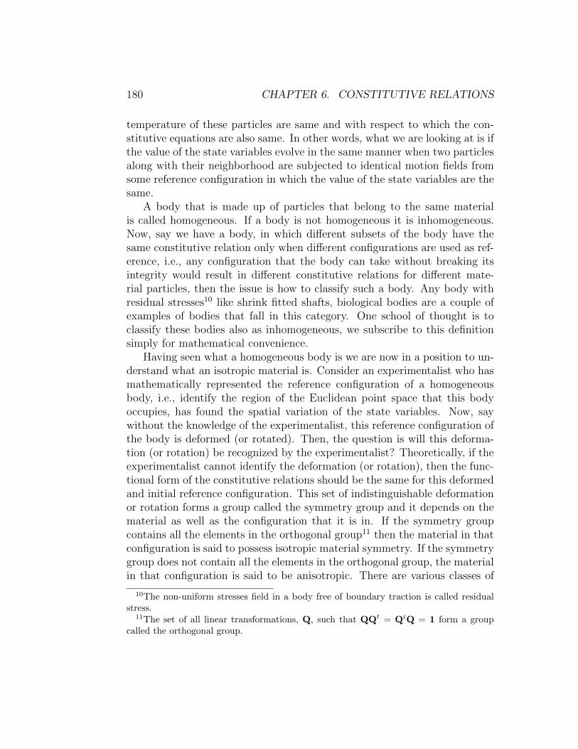
180 CHAPTER 6. CONSTITUTIVE RELATIONS
temperature of these particles are same and with respect to which the con-stitutive equations are also same. In other words, what we are looking at is ifthe value of the state variables evolve in the same manner when two particlesalong with their neighborhood are subjected to identical motion fields fromsome reference configuration in which the value of the state variables are thesame.
A body that is made up of particles that belong to the same materialis called homogeneous. If a body is not homogeneous it is inhomogeneous.Now, say we have a body, in which different subsets of the body have thesame constitutive relation only when different configurations are used as ref-erence, i.e., any configuration that the body can take without breaking itsintegrity would result in different constitutive relations for different mate-rial particles, then the issue is how to classify such a body. Any body withresidual stresses10 like shrink fitted shafts, biological bodies are a couple ofexamples of bodies that fall in this category. One school of thought is toclassify these bodies also as inhomogeneous, we subscribe to this definitionsimply for mathematical convenience.
Having seen what a homogeneous body is we are now in a position to un-derstand what an isotropic material is. Consider an experimentalist who hasmathematically represented the reference configuration of a homogeneousbody, i.e., identify the region of the Euclidean point space that this bodyoccupies, has found the spatial variation of the state variables. Now, saywithout the knowledge of the experimentalist, this reference configuration ofthe body is deformed (or rotated). Then, the question is will this deforma-tion (or rotation) be recognized by the experimentalist? Theoretically, if theexperimentalist cannot identify the deformation (or rotation), then the func-tional form of the constitutive relations should be the same for this deformedand initial reference configuration. This set of indistinguishable deformationor rotation forms a group called the symmetry group and it depends on thematerial as well as the configuration that it is in. If the symmetry groupcontains all the elements in the orthogonal group11 then the material in thatconfiguration is said to possess isotropic material symmetry. If the symmetrygroup does not contain all the elements in the orthogonal group, the materialin that configuration is said to be anisotropic. There are various classes of
10The non-uniform stresses field in a body free of boundary traction is called residualstress.
11The set of all linear transformations, Q, such that QQt = QtQ = 1 form a groupcalled the orthogonal group.

6.3. RESTRICTIONS ON CONSTITUTIVE RELATION 181
anisotropy like transversely isotropic, orthorhombic, etc., depending on theelements contained in the symmetry group.
Here we like to emphasize on some subtleties. Firstly, we emphasize thatthe symmetry group of a material depends on the configuration in which it isassessed. Thus, the material in a stress free configuration could be isotropicbut the same material in uniaxially stressed state will not be isotropic. Sec-ondly, we allow the body to be deformed because it has been shown [10] thatcertain deformations superposed on an uniaxially extended body does not al-ter the state of the body. Hence, it should be recognized that the symmetrygroup, G ⊆ H, the unimodular group12, since the volume cannot change inan equivalent placement of the body. In fact, for a perfect gas the symmetrygroup, G = H. Thirdly, unlike in the restriction due to objectivity, in thiscase only the body is rotated or deformed virtually, not its surroundings.Even though like in the restriction due to objectivity the rotation or defor-mation is virtual, it has to maintain the integrity of the body and satisfy thebalance laws, i.e., be statically admissible because the rotated or deformedconfiguration is also in equilibrium.
Now, let us mathematically investigate the restriction material symmetryimposes on the constitutive relation. Continuing with our example, σ = f(F)we examine the restriction on f(F) due to material symmetry. For any G ∈G, the restriction due to material symmetry requires that
σ = f(F) = f(FG), (6.61)
∀ F ∈ D. Of course, for this case the restriction is similar to that obtained forobjectivity (6.31), except that now, Q = 1 and Qo is not necessarily limitedto orthogonal tensors. However, for isotropic material the symmetry groupis the set of all orthogonal tensors only.
To further elucidate the difference between the restriction due to objec-tivity and material symmetry, consider a material whose response is differentalong a direction M identified in the reference configuration. Then, σ =f(F,M). Now due to objectivity we require
Qf(F,M)Qt = f(QFQto,QoM), (6.62)
for any orthogonal tensors Q and Qo and for any F ∈ D. Due to materialsymmetry we require
f(F,M) = f(FG,M), (6.63)
12The set of all linear transformations such that their determinant is positive and equalto one, form a group called the unimodular group.

182 CHAPTER 6. CONSTITUTIVE RELATIONS
∀ F ∈ D and G ∈ G. In (6.63) the right hand side is not GM because,the rotation (or deformation) G, of the reference configuration is not dis-tinguishable. In other words, G belongs to G only if GM = M. Thus, itimmediately transpires that restriction due to material symmetry (6.63) isnot same as that due to objectivity (6.62).
It is also instructive to note that if GM = M holds for any an orthog-onal tensor, G, then M = o. Thus, the result that for isotropic materialsthe response would be same in all directions and consequently there are nopreferred directions. If the material response along one direction is differ-ent, then it is called as transversely isotropic and if its response along threedirections are different, it is called orthotropic.
6.4 Isotropic Hooke’s law
Having established for isotropic materials if Cauchy stress is explicitly relatedto the deformation gradient, then this relationship would be of the form,
σ = f(F) = α01 + α1B + α2B−1, (6.64)
where αi = αi(J1, J2, J3), called the material response functions and needsto be determined from experiments. Thus, restriction due to objectivity, hasreduced the number of variables in the function from 9 to 3 and the numberof unknown functions from 6 to 3. Next, let us see if we can further reducethe number of variables that the function depends upon or the number offunctions themselves. Since, in an elastic process there is no dissipation ofenergy, this reduces the number of unknown functions to be determined tojust one and thus Cauchy stress is given by13,
σ =∂W
∂J3
1 +2
J3
[∂W
∂J1
B− ∂W
∂J2
B−1
], (6.65)
where W = W (J1, J2, J3), is called as the stored (or strain) energy per unitvolume of the reference configuration. Notice that here the stored energyfunction is the only function that needs to be determined through experi-mentation.
13Derivation of this equation is beyond the scope of this course.
6.4. ISOTROPIC HOOKE’S LAW 183
In practice, the materials undergo a non-dissipative process only when therelative displacements are small, resulting in the components of the displace-ment gradient being small. Hence, it is of interest to see the implications ofthis approximation on a general representation for Cauchy stress (6.64).
In chapter 3 (section (3.5.1), we saw that the deformation gradient isrelated to the Lagrangian and Eulerian displacement gradient as:
F = H + 1, F−1 = 1− h. (6.66)
Hence, the left Cauchy-Green deformation tensor is given by
B = H + Ht + HHt + 1, B−1 = 1− h− ht + hth. (6.67)
If tr(HHt) << 1 and tr(hht) << 1, then we could approximately calculatethe left Cauchy-Green deformation tensor as
B ≈ H + Ht + 1, B−1 ≈ 1− h− ht. (6.68)
We also saw in chapter 3 (section 3.8) that when tr(HHt) << 1 and tr(hht)<< 1, H ≈ h. Therefore we need not distinguish between the Lagrangian andEulerian linearized strain. By virtue of these approximations the expressionsin equation (6.68) can be written as:
B ≈ 2ε+ 1, B−1 ≈ 1− 2ε, (6.69)
where ε denotes the (Lagrangian or Eulerian) linearized strain tensor. Con-sequently, the invariants are calculated approximately as14
J1 ≈ 3 + 2tr(ε), J2 ≈ 3− 2tr(ε), J3 ≈ 1 + tr(ε). (6.70)
Substituting (6.69) in a general representation for stress in a isotropicmaterial, (6.64) we obtain
σ = αl01 + αl1ε. (6.71)
14The last expression is obtained by substituting (6.69) in J3 =√I2/J2 and using
Taylor’s series expansion about tr(ε) = 0, to obtain
J3 =
√I2J2
=
√J21 − tr(B2)
2J2≈
√3 + 4tr(ε)
3− 2tr(ε)≈√
1 + 2tr(ε) ≈ 1 + tr(ε).
184 CHAPTER 6. CONSTITUTIVE RELATIONS
whereαl0 = α0 + α1 + α2, αl1 = 2(α1 − α2), (6.72)
are functions of tr(ε) by virtue of (6.70). It is necessary that αl0 should be alinear function of tr(ε) and αl1 a constant; because we neglected the higherorder terms of ε to obtain the above expression. Consequently, the expressionfor Cauchy stress (6.71) simplifies to,
σ = tr(ε)λ1 + 2µε, (6.73)
where λ and µ are Lame constants and these constants alone need to bedetermined from experiments. The relation (6.73) is called the Hooke’s lawfor isotropic materials.
Since, the relation between the Cauchy stress and linearized strain islinear we can invert the constitutive relation (6.73) and write the linearizedstrain in terms of the stress as,
ε =1
2µσ − λ
2µ(3λ+ 2µ)tr(σ)1. (6.74)
Taking trace on both sides of equation (6.73) we obtain,
tr(σ) = tr(ε)[3λ+ 2µ], (6.75)
on noting that tr(·) is a linear operator and that tr(1) = 3. Thus, equation(6.74) is obtained by rearranging equation (6.73) and using equation (6.75).
Lame constants while allows one to write the constitutive relations suc-cinctly, their physical meaning and the methodology for their experimentaldetermination is not obvious. Hence, we define various material parameters,such as Young’s modulus, shear modulus, bulk modulus, Poisson’s ratio,which have a physical meaning and is easy to determine experimentally.
Before proceeding further, a few comments on the Hooke’s law has to bemade. From the derivation, it is clear that (6.73) is an approximation to thecorrect and more general (6.64). Consequently, Hooke’s law does not havesome of the characteristics one would expect a robust constitutive relationto possess. The first drawback is that contrary to the observations rigidbody rotations induces stresses in the body. To see how this happens, recallfrom chapter 3 (section 3.10.1) that linearized strain is not zero when thebody is subjected to rigid body rotations. Since, strain is not zero, it followsfrom (6.73) that stress would be present. The second drawback is that the
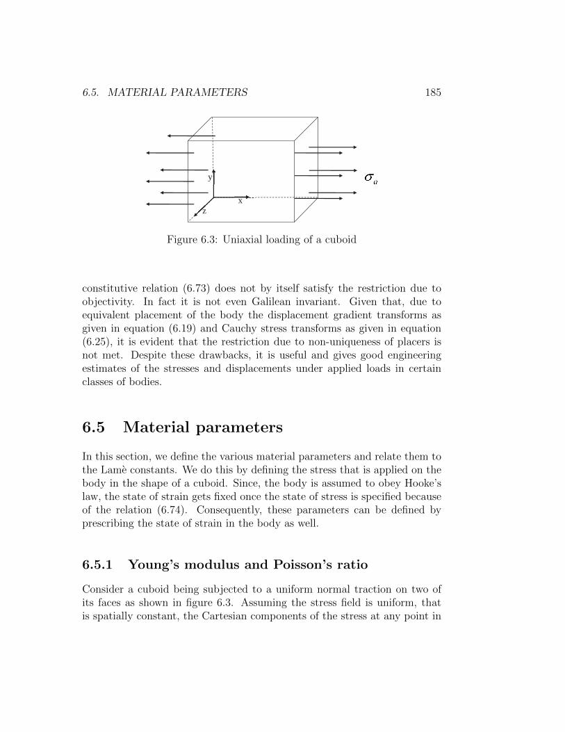
6.5. MATERIAL PARAMETERS 185
x
y
z
Figure 6.3: Uniaxial loading of a cuboid
constitutive relation (6.73) does not by itself satisfy the restriction due toobjectivity. In fact it is not even Galilean invariant. Given that, due toequivalent placement of the body the displacement gradient transforms asgiven in equation (6.19) and Cauchy stress transforms as given in equation(6.25), it is evident that the restriction due to non-uniqueness of placers isnot met. Despite these drawbacks, it is useful and gives good engineeringestimates of the stresses and displacements under applied loads in certainclasses of bodies.
6.5 Material parameters
In this section, we define the various material parameters and relate them tothe Lame constants. We do this by defining the stress that is applied on thebody in the shape of a cuboid. Since, the body is assumed to obey Hooke’slaw, the state of strain gets fixed once the state of stress is specified becauseof the relation (6.74). Consequently, these parameters can be defined byprescribing the state of strain in the body as well.
6.5.1 Young’s modulus and Poisson’s ratio
Consider a cuboid being subjected to a uniform normal traction on two ofits faces as shown in figure 6.3. Assuming the stress field is uniform, thatis spatially constant, the Cartesian components of the stress at any point in

186 CHAPTER 6. CONSTITUTIVE RELATIONS
the body is,
σ =
σa 0 00 0 00 0 0
. (6.76)
Substituting the above in equation (6.74) for the stress we obtain the strainas
ε =
12µ
[1− λ
3λ+2µ
]σa 0 0
0 − λ2µ(3λ+2µ)
σa 0
0 0 − λ2µ(3λ+2µ)
σa
(6.77)
Now, Young’s modulus, E, is defined as the ratio of the uniaxial stress to thecomponent of the linearized strain along the direction of the applied uniaxialstress, i.e.,
E =σxxεxx
=2µ
1− λ(3λ+2µ)
=µ(3λ+ 2µ)
(λ+ µ). (6.78)
The Poisson’s ratio , ν is defined as the negative of the ratio of the componentof the strain along a direction perpendicular to the axis of loading, called thetransverse strain to the component of the strain along the axis of loading,called the axial strain, i.e.,
ν = − εyyεxx
=λ
2(λ+ µ). (6.79)
In equations (6.78) and (6.79) we expressed the Young’s Modulus andPoisson’s ratio in terms of the Lame constants. This relation can be invertedto express Lame constants in terms of E and ν as,
λ =Eν
(1 + ν)(1− 2ν), µ =
E
2(1 + ν)(6.80)
Finally, substituting equation (6.80) in equation (6.73) and (6.74), theconstitutive relations can be written in terms of the Young’s modulus andPoisson’s ratio as,
σ =Eν
(1 + ν)(1− 2ν)tr(ε)1 +
E
(1 + ν)ε, (6.81)
ε =(1 + ν)
Eσ − ν
Etr(σ)1. (6.82)

6.5. MATERIAL PARAMETERS 187
6.5.2 Shear Modulus
Consider a cuboid being subjected to uniform pure shear stress of the form
σ =
0 τ 0τ 0 00 0 0
. (6.83)
Substituting the above state of stress in (6.74), the state of strain is obtainedas,
ε =1
2µ
0 τ 0τ 0 00 0 0
. (6.84)
In chapter 3, section 3.10.3, we showed that if the angle change betweentwo line segments oriented along X and Y direction is κ, then this simpleshearing deformation results in,
ε =1
2
0 κ 0κ 0 00 0 0
. (6.85)
Then, the shear modulus, G is defined as the ratio of the shear stress (τ) tochange in angle (κ) due to this applied shear stress between two orthogonalline elements in the plane of shear i.e.,
G =τ
κ= µ. (6.86)
Using equation (6.80b), the shear modulus can be written in terms of theYoung’s modulus and Poisson’s ratio as,
G =E
(1 + ν). (6.87)
6.5.3 Bulk Modulus
Consider a cuboid being subjected to uniform pure hydrostatic stress,
σ = p
1 0 00 1 00 0 1
. (6.88)

188 CHAPTER 6. CONSTITUTIVE RELATIONS
Using (6.74) it could be seen that the above state of stress result in the straintensor being,
ε =p
(3λ+ 2µ)
1 0 00 1 00 0 1
. (6.89)
The bulk modulus, K, is defined as the ratio of the mean hydrostatic stress tothe volumetric strain when the body is subjected to pure hydrostatic stress.Thus,
K =tr(σ)
3tr(ε)=
1
3(3λ+ 2µ). (6.90)
Now, we would like to express the bulk modulus in terms of Young’s modulusand Poisson’s ratio. Towards this, we substitute equation (6.80) in (6.90) toobtain
K =E
3(1− 2ν). (6.91)
6.6 Restriction on material parameters
Next, we would like to limit the range of values that these material param-eters can take so that the response predicted by using these constitutiverelations confirm with the observations.
Let us now see why Young’s and shear modulus cannot be ∞. From thedefinition of the Young’s modulus we find that the axial displacement dueto an applied axial load has to be zero if E = ∞. Similarly, if G = ∞ thechange in angle due to an applied shear stress is zero. These would happenonly if the body is rigid since, no strain develops despite stress being applied.However, the focus of the study here is deformable bodies. Hence, we obtainthe condition that E < ∞, G < ∞.
However, the bulk modulus can be ∞. From the definition of bulk mod-ulus, it is clear that if K = ∞ for some material, then the volumetric straindeveloped due to applied hydrostatic pressure, for these materials has to bezero. This means that the volume of the body made of this material does notchange, the material is incompressible. Some materials like rubber, polymersare known to be nearly incompressible. Moreover, it is also known that thevolume of these materials do not change in any deformation. This means thatthese materials are capable of undergoing only isochoric deformations. Con-stitutive relations for such incompressible materials are obtained in section

6.7. INTERNALLY CONSTRAINT MATERIALS 189
6.7.1.Since, we expect that tensile stress produce elongation and compressive
stresses produce shortening, the three modulus - Young’s, shear and bulk- should be positive. Since, E is positive, for G to be positive and finite,equation (6.87) requires (1 + ν) > 0. Thus,
ν > −1. (6.92)
Note that, this is a strict inequality because if (1 + ν) = 0, G = ∞, (since 0< E < ∞) which is not permissible.
Similarly, for K to be positive, it transpires from equation (6.91) that(1− 2ν) ≥ 0, since E is positive. Hence,
ν ≤ 0.5. (6.93)
Here we allow for equality because K can be ∞.Combining these both restrictions (6.92) and (6.93) on the Poisson’s ratio,
− 1 < ν ≤ 0.5. (6.94)
Thus, Poisson’s ratio can be negative, and it has been measured to be neg-ative for certain foams. What this means is that as the body is stretchedalong a particular direction, the cross sectional area over which the load isdistributed can increase. However, for most materials, especially metals, thiscross sectional area decreases and therefore the Poisson’s ratio is positive.
Finally, we show that the three modulus values cannot be zero. Fromthe definition of these modulus, they being zero means that, any amount ofstrain can develop even when no stress is applied. This means that there canbe displacement without the force, when the modulus value is zero. Since,there has to be force for displacement, this means that the modulus cannotbe zero.
In table 6.1 the restrictions on various parameters are summarized. Thepoint to note is that one of the Lame constants, λ has no restrictions. Fromequation (6.80), it can be seen that if 0 ≤ ν ≤ 0.5, then from the restrictionson E and ν it can be said that λ ≥ 0. However, λ < 0 for certain foamswhose Poisson’s ratio is negative. Therefore λ has no restrictions.
6.7 Internally constraint materials
Till now we have been focusing on materials that have no internal constraint,that is, if the required body force and boundary traction can be applied, any

190 CHAPTER 6. CONSTITUTIVE RELATIONS
Table 6.1: Restrictions on material parameters
Material Parameter Symbol RestrictionYoung’s modulus E 0 < E < ∞Shear modulus G 0 < G < ∞Bulk modulus K 0 < K ≤ ∞Poisson’s ratio ν −1 < ν ≤ 0.5
Lame constantµ 0 < µ < ∞λ −∞ < λ < ∞
smooth displacement field can be realized in bodies made of these materials.However, in some materials this is not true. Only smooth displacement fieldsthat satisfy certain constraints are realizable. The most common constrainton the displacement field is that it be volume preserving. Contrary to thereality, beginners tend to think that in all materials volume is preserved inall feasible deformations just because the cross sectional area reduces whenuniaxially stretched. However, this is not true. We show this next. Recol-lecting from chapter 3 (section 3.6) that the ratio of the deformed volume, vto the original volume, V in case of homogeneous deformation is given by,
v
V= det(F) ≈ 1 + tr(ε) (6.95)
where we have used equation (6.70c) to approximately compute det(F) whenthe components of the displacement gradient are small. Using equation (6.77)that gives the state of strain in the cuboid subjected to uniaxial stress, σa,the change in its volume is computed to be
v − V = V tr(ε) = Vσa
(3λ+ 2µ)= V
σa3K
= VσaE
(1− 2ν), (6.96)
where the last two equalities are obtained using equation (6.90) and (6.91).Thus, it is apparent that the volume of the cuboid changes as the magnitudeof the uniaxial stress changes when ν 6= 0.5. For physically possible val-ues of Poisson’s ratio, other than 0.5, the volume increases when uniaxiallystretched and decreases when compressed.
In this section, we outline general principle to generate constitutive re-lations for internally constrained materials. Assuming that the materials
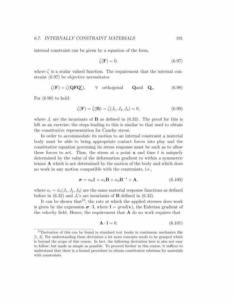
6.7. INTERNALLY CONSTRAINT MATERIALS 191
internal constraint can be given by a equation of the form,
ζ(F) = 0, (6.97)
where ζ is a scalar valued function. The requirement that the internal con-straint (6.97) be objective necessitates
ζ(F) = ζ(QFQto), ∀ orthogonal Qand Qo. (6.98)
For (6.98) to hold:
ζ(F) = ζ(B) = ζ(J1, J2, J3) = 0, (6.99)
where Ji are the invariants of B as defined in (6.33). The proof for this isleft as an exercise; the steps leading to this is similar to that used to obtainthe constitutive representation for Cauchy stress.
In order to accommodate its motion to an internal constraint a materialbody must be able to bring appropriate contact forces into play and theconstitutive equation governing its stress response must be such as to allowthese forces to act. Thus, the stress at a point x and time t is uniquelydetermined by the value of the deformation gradient to within a symmetrictensor A which is not determined by the motion of the body and which doesno work in any motion compatible with the constraints, i.e.,
σ = α01 + α1B + α2B−1 + A, (6.100)
where αi = αi(J1, J2, J3) are the same material response functions as definedbefore in (6.32) and Ji’s are invariants of B defined in (6.33).
It can be shown that15, the rate at which the applied stresses does workis given by the expression σ · l, where l = grad(v), the Eulerian gradient ofthe velocity field. Hence, the requirement that A do no work requires that
A · l = 0, (6.101)
15Derivation of this can be found in standard text books in continuum mechanics like[1, 2]. For understanding these derivation a lot more concepts needs to be grasped whichis beyond the scope of this course. In fact, the following derivation here is also not easyto follow; but made as simple as possible. To proceed further in this course, it suffices tounderstand that there is a formal procedure to obtain constitutive relations for materialswith constraints.

192 CHAPTER 6. CONSTITUTIVE RELATIONS
for all allowable motions. To relate A with ζ we take material time derivativeof (6.99) to obtain
∂ζ
∂BB · l = 0. (6.102)
Now let
A = p∂ζ
∂BB, (6.103)
where p is an arbitrary scalar to be determined from boundary conditionsand/or equilibrium equations. While it is easy to show that, the above choicefor the constraint stress satisfies the requirement (6.101), it is difficult to showthat this is the only choice and is beyond the scope of this course.
Hence, a general representation for stress with kinematic constraint (6.99)is given by
σ = α01 + α1B + α2B−1 + p
∂ζ
∂BB, (6.104)
with a undetermined scalar p to be found using equilibrium equations and/orboundary conditions.
6.7.1 Incompressible materials
As already discussed, material that can undergo only isochoric motions iscalled incompressible material. As was shown in chapter - 3 for isochoricmotions, det(F) = J3 = 1. Hence,
ζ(J1, J2, J3) = J3 − 1 = 0. (6.105)
Substituting (6.105) in (6.103) and using (2.189) we obtain
A = pJ3
2B−1B = −p∗1, (6.106)
where p∗ = −p/2. Consequently, a general representation for Cauchy stress(6.104) for incompressibility constraint reduces to,
σ = (α0 − p∗)1 + α1B + α2B−1, (6.107)
where now, αi = αi(J1, J2) since J3 is identically 1. Now introducing, p+ =−α0 + p∗, we obtain
σ = −p+1 + α1B + α2B−1, (6.108)

6.7. INTERNALLY CONSTRAINT MATERIALS 193
where without any loss of generality we assume p+ to be some arbitrary scalarto be determined from boundary conditions and/or equilibrium equations.For convenience and brevity in notation we shall drop the superscript + inp+ and write
σ = −p1 + α1B + α2B−1, (6.109)
which we consider as the most general representation for Cauchy stress in anincompressible material being subjected to elastic deformation.
As before (see section 6.4), it can be shown that when the componentsof the displacement gradient is small, the kinematical constraint equation(6.105) reduces to requiring,
tr(ε) = 0, (6.110)
and consequently the equation (6.109) can be approximated as,
σ = −p1 + 2µincε, (6.111)
where µinc is a constant material parameter and p is an arbitrary scalarto be determined from equilibrium equations and/or boundary condition.Equation (6.111) is the constitutive relation for an incompressible materialundergoing elastic deformation such that the components of the displacementgradient are small.
Before concluding this section, we would like to find the value of all thematerial parameters defined in section 6.5 for this incompressible material.
In case of the cuboid being subjected to uniaxial stress, the state of stressand strain are:
σ =
σa 0 00 0 00 0 0
, ε =
ε1 0 00 ε2 00 0 ε2
. (6.112)
The incompressibility condition (6.110) requires that
ε1 + 2ε2 = 0. (6.113)
Hence, the incompressible materials Poisson’s ratio,
νinc = −ε2ε1
= 0.5. (6.114)

194 CHAPTER 6. CONSTITUTIVE RELATIONS
Substituting (6.112) along with the requirement that ε2 = −ε1/2 obtainedfrom (6.113) for stress and strain in (6.111) we obtain:σa 0 0
0 0 00 0 0
=
−p+ 2µincε1 0 00 −p− µincε1 00 0 −p− µincε1
. (6.115)
For the above equation to hold, p = −µincε1 and hence, σa = 3µincε1. Thus,the incompressible materials Young’s modulus,
Einc =σaε1
= 3µinc. (6.116)
If the cuboid is being subjected to pure shear state of stress and strain,
σ =
0 τ 0τ 0 00 0 0
, ε =
0 κ/2 0κ/2 0 00 0 0
, (6.117)
then it is straightforward to verify that for this state of strain tr(ε) = 0and therefore the incompressibility condition (6.110) is met. Substituting,(6.117) in (6.111) we obtain:0 τ 0
τ 0 00 0 0
=
−p µincκ 0µincκ −p 0
0 0 −p
. (6.118)
For this equation to hold, p = 0 and τ = µincκ. Now, the incompressibleshear modulus is,
Ginc =τ
κ= µinc. (6.119)
Finally, if a incompressible cuboid is subjected to hydrostatic pressure,σ = −p1 and ε = 0, for the incompressibility constraint (6.110) and theconstitutive relation (6.111) to hold. Thus, incompressible materials bulkmodulus, Kinc = ∞.
Understandably there is only one material parameter in (6.111). Theincompressibility constraint (6.110) requires that νinc = 0.5 or equivalently,Kinc =∞ there by fixing one of the two independent material parameters inthe isotropic Hooke’s law.
As you would have noticed, for incompressible materials, both the state ofstress and strain are prescribed and found necessary to solve certain boundary
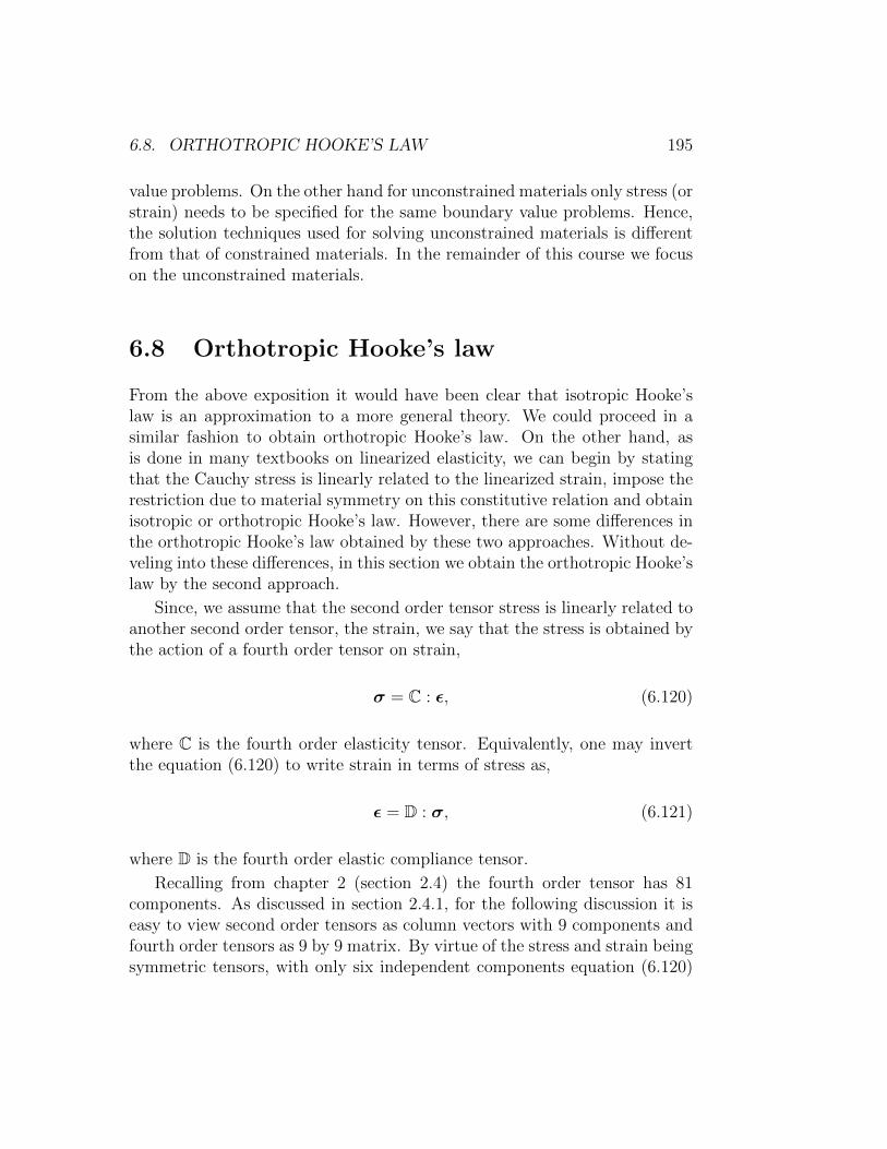
6.8. ORTHOTROPIC HOOKE’S LAW 195
value problems. On the other hand for unconstrained materials only stress (orstrain) needs to be specified for the same boundary value problems. Hence,the solution techniques used for solving unconstrained materials is differentfrom that of constrained materials. In the remainder of this course we focuson the unconstrained materials.
6.8 Orthotropic Hooke’s law
From the above exposition it would have been clear that isotropic Hooke’slaw is an approximation to a more general theory. We could proceed in asimilar fashion to obtain orthotropic Hooke’s law. On the other hand, asis done in many textbooks on linearized elasticity, we can begin by statingthat the Cauchy stress is linearly related to the linearized strain, impose therestriction due to material symmetry on this constitutive relation and obtainisotropic or orthotropic Hooke’s law. However, there are some differences inthe orthotropic Hooke’s law obtained by these two approaches. Without de-veling into these differences, in this section we obtain the orthotropic Hooke’slaw by the second approach.
Since, we assume that the second order tensor stress is linearly related toanother second order tensor, the strain, we say that the stress is obtained bythe action of a fourth order tensor on strain,
σ = C : ε, (6.120)
where C is the fourth order elasticity tensor. Equivalently, one may invertthe equation (6.120) to write strain in terms of stress as,
ε = D : σ, (6.121)
where D is the fourth order elastic compliance tensor.
Recalling from chapter 2 (section 2.4) the fourth order tensor has 81components. As discussed in section 2.4.1, for the following discussion it iseasy to view second order tensors as column vectors with 9 components andfourth order tensors as 9 by 9 matrix. By virtue of the stress and strain beingsymmetric tensors, with only six independent components equation (6.120)

196 CHAPTER 6. CONSTITUTIVE RELATIONS
can be written as,
σxxσyyσzzσxyσxzσyz
=
C11 C12 C13 C14 C15 C16
C21 C22 C23 C24 C25 C26
C31 C32 C33 C34 C35 C36
C41 C42 C43 C44 C45 C46
C51 C52 C53 C54 C55 C56
C61 C62 C63 C64 C65 C66
εxxεyyεzzεxyεxzεyz
. (6.122)
Thus, of the 81 components only 36 are independent.As stated before, since elastic process is non-dissipative, the stress is
derivable from a potential called the stored (or strain) energy, W as,
σ =∂W
∂ε, (6.123)
where W = W (ε). The above equation in index notation is given by
σi =∂W
∂εi, (6.124)
when the stress and strain tensors are represented as column vectors with sixcomponents. Now, σ1 = σxx, σ2 = σyy, σ3 = σzz, σ4 = σxy, σ5 = σxz, σ6 =σyz and ε1 = εxx, ε2 = εyy, ε3 = εzz, ε4 = εxy, ε5 = εxz, ε6 = εyz. This is justa change in notation.
It follows from (6.120) that the elasticity tensor could be obtained from
C =∂σ
∂ε, in index notation (C)ij =
∂σi∂εj
. (6.125)
Substituting (6.124) in the above equation,
Cij =∂2W
∂εj∂εi. (6.126)
Thus, if W is a smooth function of strain, which it is, then the order of differ-entiation would not matter. Hence, elasticity tensor would be a symmetricfourth order tensor. This means that the number of independent componentsin C reduces from 36 to 21 components.
Further reduction in the number of independent components of the elas-ticity tensor cannot be done by restriction due to non-uniqueness of placers

6.8. ORTHOTROPIC HOOKE’S LAW 197
argument. Given that, due to equivalent placement of the body the dis-placement gradient transforms as given in equation (6.19) and Cauchy stresstransforms as given in equation (6.25), it is evident that the restriction dueto non-uniqueness of placers is not met by the constitutive relation (6.120).Then, due to changes in the coordinate basis, the elasticity tensor shouldtransforms as
Cijkl = QiaQjbQkcQldCabcd, (6.127)
according to the transformation law for fourth order tensor (see section 2.6).Ideally we should require that the components of the elasticity tensor be thesame irrespective of the choice of the basis. In other words, this means, asdiscussed in section 2.6.3, that the elasticity tensor should be the isotropicfourth order tensor. Since, the elasticity fourth order tensor is symmetric, inthe general representation for the isotropic fourth order tensor (2.165), γ =β = µ and thus,
C = λ1⊗ 1 + µ[I + I], (6.128)
where we have replaced the constant α with λ. This λ and µ are the sameLame constants. Writing (6.128) in matrix form,
C =
λ+ 2µ λ λ 0 0 0λ λ+ 2µ λ 0 0 0λ λ λ+ 2µ 0 0 00 0 0 2µ 0 00 0 0 0 2µ 00 0 0 0 0 2µ
. (6.129)
Thus, we have obtained the isotropic form of the Hooke’s law.Contrary to this ideal requirement, it is required that the components of
the elasticity tensor be the same only for certain equivalent choices of thebasis vectors. A material with three mutually perpendicular planes of sym-metry is called orthotropic. This means that 180 degree rotation about eachof the coordinate basis should not change the components of the elasticitytensor. Thus, for an orthotropic material the components of C must be sameas that of C in (6.127) for the following choices of Qpq:
[Q]pq =
−1 0 00 −1 00 0 1
, [Q]pq =
1 0 00 −1 00 0 −1
, [Q]pq =
−1 0 00 1 00 0 −1
.
(6.130)

198 CHAPTER 6. CONSTITUTIVE RELATIONS
It can be seen that as a result of this condition, the number of independentcomponents in the elasticity tensor reduces from 21 to 9 for an orthotropicmaterial and hence C for an orthotropic material is given by:
C =
C1 C2 C3 0 0 0C2 C4 C5 0 0 0C3 C4 C6 0 0 00 0 0 C7 0 00 0 0 0 C8 00 0 0 0 0 C9
, (6.131)
where C1, C2, . . ., C9 are material parameters.Similarly, for other equivalent choices of the basis vector, we obtain dif-
ferent forms for the elasticity tensor.One can now define material parameters like Young’s modulus, Poisson’s
ratio, shear modulus and elaborate on the experiments that needs to be doneto estimate the 9 constants characterizing the orthotropic material. Then,one can look at restrictions on them. Instead of doing these, we now focuson solving boundary value problems involving isotropic materials that obeyHooke’s law.
6.9 Summary
In this chapter, we saw what a constitutive relation is? why do we needconstitutive relations? Then we understood what we mean by an elastic re-sponse. This was followed by a discussion on the general restrictions thatthe constitutive relation has to satisfy and its application to get a generalrepresentation for Cauchy stress in an isotropic material undergoing elas-tic process. When the components of the displacement gradient are small,we showed that this general representation reduces to isotropic Hooke’s law.Then, we introduced the various material parameters used to express theHooke’s law and established the relationship between them. We also foundphysically reasonable range of values that these parameters can take. Whileall these were dealt with in detail, we looked briefly on how to obtain con-stitutive relations for materials with constraints. As an illustration of thismethodology, we obtained the constitutive relation for incompressible mate-rials, materials which undergo only isochoric deformations. Finally, we alsoderived the Hooke’s law for orthotropic materials. The one equation that

6.10. SELF-EVALUATION 199
should be remembered from this chapter is:
σ = λtr(ε)1 + 2µε. (6.132)
6.10 Self-Evaluation
1. A body in the form of a cube of side 10 cm is subjected to a deformationof the form: x = (1+a1)X+a2Y , y = (1+a3)Y , z = (1+a4)Z, where ai’sare constants and (X, Y, Z) are the Cartesian coordinates of a materialpoint before deformation and (x, y, z) are the Cartesian coordinates ofthe same material point after deformation. If the Cauchy stress, σis related to the deformation gradient, F, through σ = µ[1 − FFt],where µ is a constant. Find the (a) Cauchy stress, (b) First Piola-Krichhoff stress, and (c) Second Piola-Krichhoff stress, for the abovedeformations. Then, show that all these three stresses are nearly thesame when ai’s are small.
2. Show that a plane stress state will result in a plane strain state onlywhen tr(σ) = 0 in a material that obeys isotropic Hooke’s law. Rec-ollect that this state of stress wherein tr(σ) = 0 is called pure shearstate of stress.
3. Show that a plane strain state will result in a plane stress state onlywhen tr(ε) = 0 in a material that obeys isotropic Hooke’s law.
4. Find the relationship between shear modulus, bulk modulus and Pois-son’s ratio.
5. A cube of side 1 cm, defined by B = (X, Y, Z)|0 ≤ X ≤ 1cm, 0 ≤Y ≤ 1cm, 0 ≤ Z ≤ 1cm obeying isotropic Hooke’s law with Young’smodulus, E = 200 GPa and Poisson’s ratio, ν = 0.3 is subjected to anuniform Cauchy stress,
σ =
−100 50 050 100 00 0 0
MPa,
corresponding to an orthonormal Cartesian basis (ex, ey, ez). Forthis cube:

200 CHAPTER 6. CONSTITUTIVE RELATIONS
(a) Determine the linearized strain, ε
(b) Determine the displacement vector given that the displacement ofthe point (0, 0, 0), u(0, 0, 0) = o and that of the point (0, 0, 1) isu(0, 0, 1) = o .
(c) Determine the location of the particle originally at Cartesian co-ordinates (1, 0, 1)
(d) Determine the location of the particle in the reference configura-tion, if its current Cartesian coordinates are (1, 0, 1)
(e) Determine the displacement of the particle originally at Cartesiancoordinates (1, 0, 1)
(f) Determine the displacement of the particle currently at Cartesiancoordinates (1, 0, 1)
(g) Calculate the change in the angle between two line segments ini-tially oriented along ey and ez directions in the reference configu-ration
(h) Calculate the change in the volume of the cube
(i) Calculate the deformed surface area and its orientation for eachof the six faces of a cube
(j) Calculate the change in length of the straight line segments oflength 1 mm oriented initially along (i) ex (ii) ey (iii) (ex+ey)/
√2
(k) Determine the displaced location of the material particles whichoriginally comprise
(i) The plane circular surface Z = 0, X2 + Y 2 = 0.25,
(ii) The plane elliptical surface Z = 0, 9X2 + 4Y 2 = 1.
(iii) The plane elliptical surface Z = 0, 4X2 + 9Y 2 = 1.
(l) Sketch the displaced configurations for (i), (ii) and (iii) in theabove problem.
(m) Sketch the deformed configuration of the cube.
6. A cube of side 1 cm, defined by B = (X, Y, Z)|0 ≤ X ≤ 1cm, 0 ≤Y ≤ 1cm, 0 ≤ Z ≤ 1cm obeying isotropic Hooke’s law with Young’smodulus, E = 200 GPa and Poisson’s ratio, ν = 0.3 is subjected to an
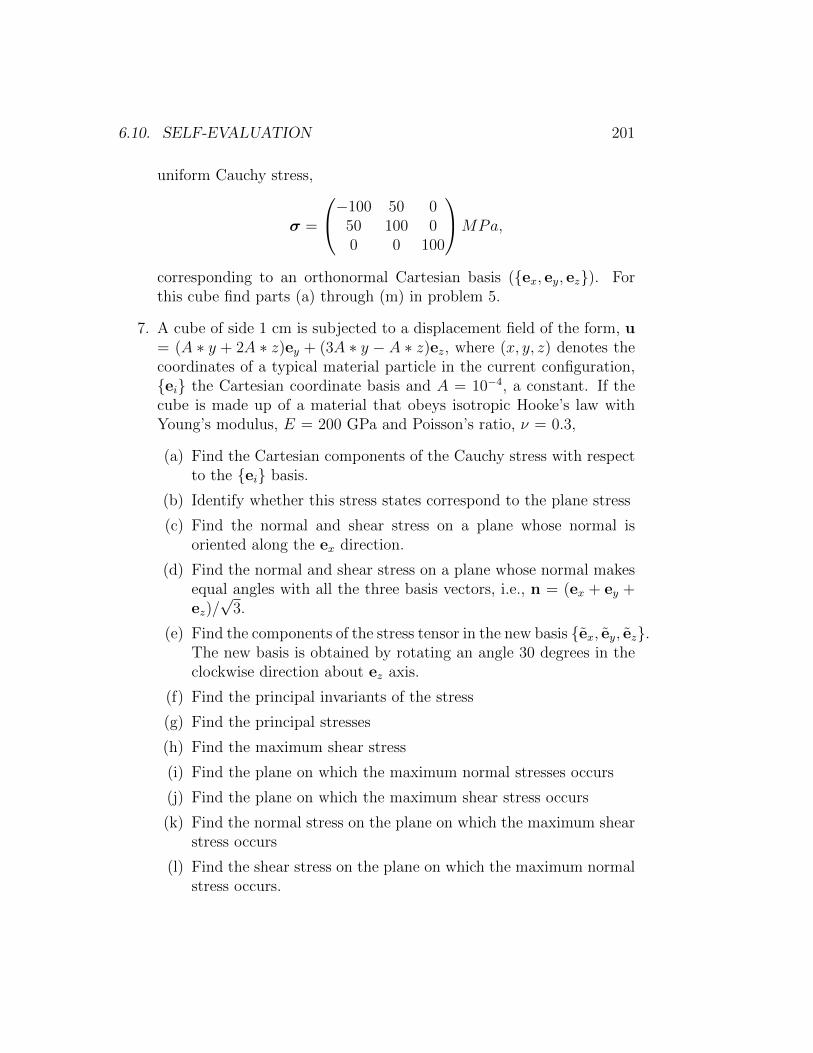
6.10. SELF-EVALUATION 201
uniform Cauchy stress,
σ =
−100 50 050 100 00 0 100
MPa,
corresponding to an orthonormal Cartesian basis (ex, ey, ez). Forthis cube find parts (a) through (m) in problem 5.
7. A cube of side 1 cm is subjected to a displacement field of the form, u= (A ∗ y + 2A ∗ z)ey + (3A ∗ y − A ∗ z)ez, where (x, y, z) denotes thecoordinates of a typical material particle in the current configuration,ei the Cartesian coordinate basis and A = 10−4, a constant. If thecube is made up of a material that obeys isotropic Hooke’s law withYoung’s modulus, E = 200 GPa and Poisson’s ratio, ν = 0.3,
(a) Find the Cartesian components of the Cauchy stress with respectto the ei basis.
(b) Identify whether this stress states correspond to the plane stress
(c) Find the normal and shear stress on a plane whose normal isoriented along the ex direction.
(d) Find the normal and shear stress on a plane whose normal makesequal angles with all the three basis vectors, i.e., n = (ex + ey +ez)/√
3.
(e) Find the components of the stress tensor in the new basis ex, ey, ez.The new basis is obtained by rotating an angle 30 degrees in theclockwise direction about ez axis.
(f) Find the principal invariants of the stress
(g) Find the principal stresses
(h) Find the maximum shear stress
(i) Find the plane on which the maximum normal stresses occurs
(j) Find the plane on which the maximum shear stress occurs
(k) Find the normal stress on the plane on which the maximum shearstress occurs
(l) Find the shear stress on the plane on which the maximum normalstress occurs.
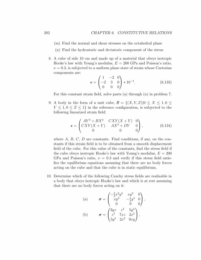
202 CHAPTER 6. CONSTITUTIVE RELATIONS
(m) Find the normal and shear stresses on the octahedral plane
(n) Find the hydrostatic and deviatoric component of the stress
8. A cube of side 10 cm and made up of a material that obeys isotropicHooke’s law with Young’s modulus, E = 200 GPa and Poisson’s ratio,ν = 0.3, is subjected to a uniform plane state of strain whose Cartesiancomponents are:
ε =
1 −2 0−2 3 00 0 0
∗ 10−4. (6.133)
For this constant strain field, solve parts (a) through (n) in problem 7.
9. A body in the form of a unit cube, B = (X, Y, Z)|0 ≤ X ≤ 1, 0 ≤Y ≤ 1, 0 ≤ Z ≤ 1 in the reference configuration, is subjected to thefollowing linearized strain field:
ε =
AY 3 +BX2 CXY (X + Y ) 0CXY (X + Y ) AX3 +DY 0
0 0 0
, (6.134)
where A, B, C, D are constants. Find conditions, if any, on the con-stants if this strain field is to be obtained from a smooth displacementfield of the cube. For this value of the constants, find the stress field ifthe cube obeys isotropic Hooke’s law with Young’s modulus, E = 200GPa and Poisson’s ratio, ν = 0.3 and verify if this stress field satis-fies the equilibrium equations assuming that there are no body forcesacting on the cube and that the cube is in static equilibrium.
10. Determine which of the following Cauchy stress fields are realizable ina body that obeys isotropic Hooke’s law and which is at rest assumingthat there are no body forces acting on it:
(a) σ =
−32x2y2 xy3 0xy3 −1
4y4 0
0 0 0
,
(b) σ =
3yz z2 5y2
z2 7xz 2x2
5y2 2x2 9xy
,

6.10. SELF-EVALUATION 203
(c) σ =
3x+ 5y 7x− 3y 07x− 3y 2x− 7y 0
0 0 0
,
(d) σ =
3x −3y 0−7x 7y 0
0 0 0
,
where the components of the stress are with respect to orthonormalCartesian basis and (x, y, z) denote the Cartesian coordinates of a typ-ical material particle in the current configuration of the body. Recollectthat for a stress field to be realizable in a body it should not only satisfythe equilibrium equations but also the compatibility conditions.

204 CHAPTER 6. CONSTITUTIVE RELATIONS

Chapter 7
Boundary Value Problem:Formulation
7.1 Overview
In the previous chapters, we mastered the basic concepts of strain and stressalong with the four basic equations, namely, the strain-displacement relation,compatibility condition, constitutive relation and the equilibrium equations.We are now in a position to find the stresses and displacement throughoutthe body - in the interior as well as in its boundary - given the displacementover some part of the boundary of the body and the traction on some otherpart of the boundary. Usually the part of the boundary where traction isspecified, displacement would not be given and vice versa. In this course weshall formulate the boundary value problem for a body made up of isotropicmaterial obeying Hooke’s law and deforming in such a manner that the rel-ative displacement between its particles is small1. Then, we discuss threestrategies to solve this boundary value problem.
Before we endeavor on the formulation of the boundary value problemand discuss strategies to solve it, we recollect and record the basic equations.If u represents the displacement that the particles undergo from a stressfree reference configuration to the deformed current configuration with thedeformation taking place due to application of the traction on the boundary,
1This condition is to ensure that the components of the displacement gradient is small.
205

206 CHAPTER 7. BOUNDARY VALUE PROBLEM: FORMULATION
then we define the linearized strain as,
ε =1
2[h + ht], (7.1)
where, h = grad(u). The equation (7.1) is called as the strain displacementrelation. The constitutive relation that relates the stress to the strain that isto be used in this course is the Hooke’s law. The various forms of the sameHooke’s law that would be used is recorded:
σ = λtr(ε)1 + 2µε, (7.2)
σ =E
(1 + ν)
[ν
(1− 2ν)tr(ε)1 + ε
], (7.3)
ε =(1 + ν)
Eσ − ν
Etr(σ)1, (7.4)
where σ is the Cauchy stress, λ and µ are Lame constants and E is theYoung’s modulus and ν is the Poisson’s ratio. The conservation of linearmomentum equation,
div(σ) + ρ(b− a) = o, (7.5)
where ρ is the density, b is the body force per unit mass and a is the accel-eration, for our purposes here reduces to:
div(σ) = o, (7.6)
since we have ignored the body forces and look at configurations that arein static equilibrium under the action of the applied static traction. That isthe displacement is assumed not to depend on time. It is appropriate thatwe discuss these assumptions in some detail. By ignoring the body forces weare ignoring the stresses that arise in the body due to its own mass. Since,these stresses are expected to be much small in comparison to the stressesinduced in the body due to traction acting on its boundary and these stressespractically do not vary over the surface of the earth, ignoring the body forcesis justifiable. In the same spirit, all that we require is that the magnitude ofacceleration be small, if not zero.
Finally, we document the compatibility conditions; the conditions that

7.2. FORMULATION OF BOUNDARY VALUE PROBLEM 207
ensures the existence of a smooth displacement field given a strain field:
∂2εxx∂y2
+∂2εyy∂x2
= 2∂2εxy∂x∂y
(7.7)
∂2εyy∂z2
+∂2εzz∂y2
= 2∂2εyz∂y∂z
(7.8)
∂2εxx∂z2
+∂2εzz∂x2
= 2∂2εxz∂x∂z
(7.9)
∂
∂y
(∂εxy∂z
+∂εyz∂x− ∂εxz
∂y
)=
∂2εyy∂z∂x
(7.10)
∂
∂z
(∂εyz∂x
+∂εxz∂y− ∂εxy
∂z
)=
∂2εzz∂x∂y
(7.11)
∂
∂x
(∂εxz∂y
+∂εxy∂z− ∂εyz
∂x
)=
∂2εxx∂y∂z
(7.12)
7.2 Formulation of boundary value problem
Formulation of the boundary value problem involves specification of the ge-ometry of the body, the constitutive relation and the boundary conditions.To elaborate, we have to define the region of the Euclidean point spacethe body occupies in the reference configuration, which is denoted by B.For example, the body might occupy a region that is a unit cube, then us-ing Cartesian coordinates the body is defined as B = (X, Y, Z)|0 ≤ X ≤1, 0 ≤ Y ≤ 1, 0 ≤ Z ≤ 1. Alternatively, the body might be the annularregion between two annular cylinders of radius Ro and Ri and height H,then using cylindrical polar coordinates the body may be defined as B =(R,Θ, Z)|Ri ≤ R ≤ Ro, 0 ≤ Θ ≤ 2π, 0 ≤ Z ≤ H. The boundary of thebody, denoted as ∂B is a surface that encloses the body. For illustration,in the cube example, the surface is composite of 6 different planes, definedby X = 0, X = 1, Y = 0, Y = 1, Z = 0 and Z = 1 respectively and inthe annular cylinder example the surface is composed of 4 different planes,defined by R = Ri, R = Ro, Z = 0, Z = H.
In this course, at least, the constitutive relation is known; it is Hooke’slaw for isotropic materials. In real life problem, the weakest link in theformulation of the boundary value problem is the constitutive relation.
Then finally one needs to prescribe boundary conditions. These are speci-fications of the displacement or traction on the surface of the body. Depend-
208 CHAPTER 7. BOUNDARY VALUE PROBLEM: FORMULATION
ing on what is prescribed on the surface, there are four type of boundaryconditions. They are
1. Displacement boundary condition: Here the displacement is spec-ified on the entire boundary of the body. This is also called as Dirichletboundary condition
2. Traction boundary condition: Here the traction is specified on theentire boundary of the body. This is also called as Neumann boundarycondition
3. Mixed boundary condition: Here the displacement is specified onpart of the boundary and traction is specified on the remaining part ofthe boundary. Both traction as well as displacement are not specifiedover any part of boundary
4. Robin boundary condition: Here both the displacement and thetraction are specified on the same part of the boundary.
Once, the geometry of the body, constitutive relations and boundaryconditions are prescribed then finding the Cauchy stress and displacementover the entire region of the body such that the displacement is continuousand differentiable over the entire region occupied by the body and the stresscomputed using this displacement field from the constitutive relation satisfiesthe equilibrium equations is called as solving the boundary value problem.If for a given geometry of the body, constitutive relations and boundaryconditions, there exists only one displacement and stress field as a solutionto the boundary value problem then the solution to the boundary valueproblem is said to be unique.
Now it is appropriate to make a few comments regarding the choice of theindependent variable for the boundary value problem. That is, when we saythe region occupied by the body, we should have been more specific and saidwhether this is the region occupied by the body in the reference or currentconfiguration. As described in section 3.4 of chapter 3, the displacement andthe stresses can be given an Eulerian or Lagrangian description, i.e.,
u = u(X) = u(x), σ = σ(X) = σ(x). (7.13)
In this course, to be specific, we follow the Eulerian description of these fields.That is we use the region occupied by the body in the current configuration
7.3. TECHNIQUES TO SOLVE BOUNDARY VALUE PROBLEMS 209
as the spatial domain of the boundary value problem. However, this domainis not known a priori. Therefore, we approximate the region occupied bythe body in the current configuration with the region occupied by the bodyin the reference configuration. This approximation is justified, since we areinterested only in problems where the components of the gradient of thedisplacement field are small and the magnitude of the displacement is alsosmall. Then, one might ponder as to why we cannot say we are following theLagrangian description of these fields. In chapter 5 section 5.4.1, we showedthat the conservation of linear momentum takes different forms dependingon the description of the stress field. The equation used here (7.5) is de-rived assuming Eulerian or spatial description of the stress field. If we use(5.46) instead of (7.5) then we would have said we are following Lagrangiandescription of these fields. Following Lagrangian description also, we wouldobtain the same governing equations if we assume that the components ofthe gradient of the deformation field are small and the magnitude of thedisplacement is small; but we have to do a little more algebra than sayingupfront that we are following an Eulerian or spatial description.
7.3 Techniques to solve boundary value prob-
lems
Depending on the boundary condition specified the solution can be found us-ing one of the following two techniques. Outline of these methods is presentednext.
7.3.1 Displacement method
Here we take the displacement field as the basic unknown that need to bedetermined. Then using this displacement field we find the strain using thestrain displacement relation (7.1). The so computed strain is substituted inthe constitutive relation written using Lame constants (7.2) to obtain
σ = λdiv(u)1 + µ[grad(u) + grad(u)t
], (7.14)
where we have used the definition of divergence operator, (2.208) and theproperty of the trace operator (2.67). Substituting (7.14) in the reducedequilibrium equations, under the assumption that body forces can be ignored

210 CHAPTER 7. BOUNDARY VALUE PROBLEM: FORMULATION
and the body is in static equilibrium, (7.5) we obtain
(λ+µ)grad(div(u))+µ∆u+div(u)grad(λ)+2εgrad(µ)+ρb = ρD2u
Dt2, (7.15)
where we have used equation (3.31) to write the acceleration in terms of the
displacement and D(·)DtE denotes the total time derivative. In addition, to
obtain the equation (7.15), we have used the following identities:
1. Since divergence is a linear operator,
div(λdiv(u)1 + 2µε) = div(λdiv(u)1) + div(2µε), (7.16)
2. It follows from equation (2.218) that
div(λdiv(u)1) = grad(λdiv(u)), (7.17)
div(2µε) = 2εgrad(µ) + µ[div(grad(u)) + div((grad(u))t)
],
(7.18)
where we have used the fact that div is a linear operator and 1m = mwhen m is any vector and 1 is the second order identity tensor.
3. From the identity (2.222) it follows that,
grad(λdiv(u)) = grad(λ)div(u) + λgrad(div(u)). (7.19)
4. Using definition of the Laplace operator (2.212)
div(grad(u)) = ∆u. (7.20)
5. Using the identity (2.211) we note that
div((grad(u))t) = grad(div(u)). (7.21)
Thus, we obtain (7.15) by substituting successive substitution of equations(7.17) through (7.21) in (7.16).
In order to simplify equation (7.15), we make the following assumptions:
1. The body is homogeneous. Hence λ and µ are constants

7.3. TECHNIQUES TO SOLVE BOUNDARY VALUE PROBLEMS 211
2. Body forces can be ignored
3. Body is in static equilibrium under the applied traction
In lieu of these assumptions, equation (7.15) reduces to
(λ+ µ)grad(div(u)) + µ∆u = o. (7.22)
If body forces cannot be ignored but the other two assumptions hold, then(7.15) reduces to
(λ+ µ)grad(div(u)) + µ∆u + ρb = o. (7.23)
In this course, we attempt to find the displacement field that satisfies (7.22)along with the prescribed boundary conditions. We compute the stress fieldcorresponding to the determined displacement field, using equation (7.2)where the strain is related to the displacement field through equation (7.1).We illustrate this method in section 7.4.1.
7.3.2 Stress method
Here we use stress as the basic unknown that needs to be determined. Thismethod is applicable only for cases when the inertial forces (ρa) can beneglected. Since, we have assumed stress as the basic unknown, we wantto express the compatibility conditions (7.7) through (7.12) in terms of thestresses. For this we compute the strains in terms of the stresses using theconstitutive relation (7.4) and substitute in the compatibility conditions toobtain the following 6 equations:
(1− ν)
[∂2σxx∂y2
+∂2σyy∂x2
]− ν
[∂2σzz∂x2
+∂2σzz∂y2
]= 2(1 + ν)
∂2σxy∂x∂y
, (7.24)
(1− ν)
[∂2σyy∂z2
+∂2σzz∂y2
]− ν
[∂2σxx∂y2
+∂2σxx∂z2
]= 2(1 + ν)
∂2σyz∂y∂z
, (7.25)
(1− ν)
[∂2σxx∂z2
+∂2σzz∂x2
]− ν
[∂2σyy∂x2
+∂2σyy∂z2
]= 2(1 + ν)
∂2σxz∂x∂z
, (7.26)
2(1 + ν)∂
∂y
(∂σxy∂z
+∂σyz∂x− ∂σxz
∂y
)=
∂2
∂z∂x(σyy − ν[σxx + σzz]) , (7.27)
2(1 + ν)∂
∂z
(∂σyz∂x
+∂σxz∂y− ∂σxy
∂z
)=
∂2
∂x∂y(σzz − ν[σxx + σyy]) , (7.28)
2(1 + ν)∂
∂x
(∂σxy∂z
+∂σxz∂y− ∂σyz
∂x
)=
∂2
∂y∂z(σxx − ν[σyy + σzz]) , (7.29)

212 CHAPTER 7. BOUNDARY VALUE PROBLEM: FORMULATION
where we have assumed that the body is homogeneous and hence Young’smodulus, E and Poisson’s ratio, ν do not vary spatially. Now, we have tofind the 6 components of the stress such that the 6 equations (7.24) through(7.29) holds along with the three equilibrium equations
∂σxx∂x
+∂σxy∂y
+∂σxz∂z
+ ρbx = 0, (7.30)
∂σxy∂x
+∂σyy∂y
+∂σyz∂z
+ ρby = 0, (7.31)
∂σxz∂x
+∂σyz∂y
+∂σzz∂z
+ ρbz = 0, (7.32)
where bi’s are the Cartesian components of the body forces. The aboveequilibrium equations (7.30) through (7.32) are obtained from (7.5) by settinga = o.
If the body forces could be obtained from a potential, β = β(x, y, z) calledas the load potential, as
b = −1
ρgrad(β), (7.33)
then the Cartesian components of the Cauchy stress could be obtained froma potential, φ = φ(x, y, z) called as the Airy’s stress potential and the loadpotential, β as,
σ =
∂2φ∂y2
+ ∂2φ∂z2
+ β − ∂2φ∂x∂y
− ∂2φ∂x∂z
− ∂2φ∂x∂y
∂2φ∂x2
+ ∂2φ∂z2
+ β − ∂2φ∂y∂z
− ∂2φ∂x∂z
− ∂2φ∂y∂z
∂2φ∂x2
+ ∂2φ∂y2
+ β
, (7.34)
so that the equilibrium equations (7.30) through (7.32) is satisfied for anychoice of φ. Substituting for the Cartesian components of the stress fromequation (7.34) in the compatibility equations (7.24) through (7.29) and sim-plifying we obtain:
(1− 2ν)
(ν − 1)
[∂4φ
∂x4+
∂4φ
∂x2∂y2+∂4φ
∂y4+∂2β
∂x2+∂2β
∂y2
]=
∂2
∂z2
[∂2φ
∂x2+∂2φ
∂y2
],(7.35)
(1− 2ν)
(ν − 1)
[∂4φ
∂y4+
∂4φ
∂y2∂z2+∂4φ
∂z4+∂2β
∂y2+∂2β
∂z2
]=
∂2
∂x2
[∂2φ
∂y2+∂2φ
∂z2
],(7.36)
(1− 2ν)
(ν − 1)
[∂4φ
∂x4+
∂4φ
∂x2∂z2+∂4φ
∂z4+∂2β
∂x2+∂2β
∂z2
]=
∂2
∂y2
[∂2φ
∂x2+∂2φ
∂z2
],(7.37)
7.3. TECHNIQUES TO SOLVE BOUNDARY VALUE PROBLEMS 213
∂2
∂x∂z
[2∂2φ
∂y2+ (1− ν)
∂2φ
∂x2+∂2φ
∂z2
+ (1− 2ν)β
]= 0, (7.38)
∂2
∂x∂y
[2∂2φ
∂z2+ (1− ν)
∂2φ
∂x2+∂2φ
∂y2
+ (1− 2ν)β
]= 0, (7.39)
∂2
∂y∂z
[2∂2φ
∂x2+ (1− ν)
∂2φ
∂y2+∂2φ
∂z2
+ (1− 2ν)β
]= 0. (7.40)
Thus, a potential that satisfies equations (7.35) through (7.40) and the pre-scribed boundary conditions is said to be the solution to the given boundaryvalue problem. Once the Airy’s stress potential is obtained, the stress fieldcould be computed using (7.34). Using this stress field the strain field iscomputed using the constitutive relation (7.4). From this strain field, thesmooth displacement field is obtained by integrating the strain displacementrelation (7.1).
Plane stress formulation
Next, we specialize the above stress formulation for the plane stress case.Without loss of generality, let us assume that the Cartesian components ofthis plane stress state is
σ =
σxx σxy 0σxy σyy 00 0 0
. (7.41)
Further, let us assume that body forces are absent and that the Airy’s stressfunction depends on only x and y. Thus, β = 0 and φ = φ(x, y). Notethat this assumption for the Airy’s stress function does not ensure σzz = 0,whenever ∂2φ
∂x2+ ∂2φ
∂y26= 0. Hence, plane stress formulation is not a specializa-
tion of the general 3D problem. Therefore, we have to derive the governingequations again following the same procedure.
Since, we assume that there are no body forces and the Airy’s stressfunction depends only on x and y, the Cartesian components of the stressare related to the Airy’s stress function as,
σ =
∂2φ∂y2
− ∂2φ∂x∂y
0
− ∂2φ∂x∂y
∂2φ∂x2
0
0 0 0
. (7.42)
214 CHAPTER 7. BOUNDARY VALUE PROBLEM: FORMULATION
Substituting for stress from equation (7.42) in the constitutive relation (7.4)we obtain,
ε =1
E
∂2φ∂y2− ν ∂2φ
∂x2−(1 + ν) ∂2φ
∂x∂y0
−(1 + ν) ∂2φ∂x∂y
∂2φ∂x2− ν ∂2φ
∂y20
0 0 −ν[∂2φ∂x2
+ ∂2φ∂y2
] . (7.43)
Substituting for strain from equation (7.43) in the compatibility condition(7.7) through (7.12), the non-trivial equations are
∂4φ
∂y4+∂4φ
∂x4+ 2
∂4φ
∂x2∂y2= 0, (7.44)
∂2
∂y2
[∂2φ
∂x2+∂2φ
∂y2
]= 0, (7.45)
∂2
∂x2
[∂2φ
∂x2+∂2φ
∂y2
]= 0, (7.46)
∂2
∂x∂y
[∂2φ
∂x2+∂2φ
∂y2
]= 0, (7.47)
Now, for equations (7.45) through (7.47) to hold,
∂2φ
∂x2+∂2φ
∂y2= α1x+ α2y + α3, (7.48)
where αi’s are constants. Differentiating equation (7.48) with respect to xtwice and adding to this the result of differentiation of equation (7.48) withrespect to y twice, we obtain equation (7.44). Thus, for equations (7.44)through (7.47) to hold it suffices that φ satisfy equation (7.48) along withthe prescribed boundary conditions. Comparing the expression for εzz inequation (7.43) and the requirement (7.48) arising from compatibility equa-tions (7.8), (7.9) and (7.11) is a restriction on how the out of plane normalstrain can vary, i.e., εzz = α1x + α2y + α3, where αi’s are some constants.Hence, this requirement that φ satisfy equation (7.48) does not lead to solu-tion of a variety of boundary value problems. Due to Poisson’s effect planestress does not lead to plane strain and vice versa, resulting in the presentdifficulty. To overcome this difficulty, it has been suggested that for planeproblems one should use the 2 dimensional constitutive relations, instead of3 dimensional constitutive relations that we have been using till now.
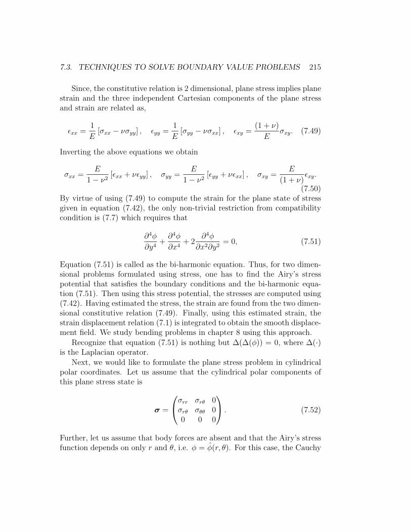
7.3. TECHNIQUES TO SOLVE BOUNDARY VALUE PROBLEMS 215
Since, the constitutive relation is 2 dimensional, plane stress implies planestrain and the three independent Cartesian components of the plane stressand strain are related as,
εxx =1
E[σxx − νσyy] , εyy =
1
E[σyy − νσxx] , εxy =
(1 + ν)
Eσxy. (7.49)
Inverting the above equations we obtain
σxx =E
1− ν2[εxx + νεyy] , σyy =
E
1− ν2[εyy + νεxx] , σxy =
E
(1 + ν)εxy.
(7.50)By virtue of using (7.49) to compute the strain for the plane state of stressgiven in equation (7.42), the only non-trivial restriction from compatibilitycondition is (7.7) which requires that
∂4φ
∂y4+∂4φ
∂x4+ 2
∂4φ
∂x2∂y2= 0, (7.51)
Equation (7.51) is called as the bi-harmonic equation. Thus, for two dimen-sional problems formulated using stress, one has to find the Airy’s stresspotential that satisfies the boundary conditions and the bi-harmonic equa-tion (7.51). Then using this stress potential, the stresses are computed using(7.42). Having estimated the stress, the strain are found from the two dimen-sional constitutive relation (7.49). Finally, using this estimated strain, thestrain displacement relation (7.1) is integrated to obtain the smooth displace-ment field. We study bending problems in chapter 8 using this approach.
Recognize that equation (7.51) is nothing but ∆(∆(φ)) = 0, where ∆(·)is the Laplacian operator.
Next, we would like to formulate the plane stress problem in cylindricalpolar coordinates. Let us assume that the cylindrical polar components ofthis plane stress state is
σ =
σrr σrθ 0σrθ σθθ 00 0 0
. (7.52)
Further, let us assume that body forces are absent and that the Airy’s stressfunction depends on only r and θ, i.e. φ = φ(r, θ). For this case, the Cauchy
216 CHAPTER 7. BOUNDARY VALUE PROBLEM: FORMULATION
stress cylindrical polar components are assumed to be
σ =
1r∂φ∂r
+ 1r2∂2φ∂θ2
− ∂∂r
(1r∂φ∂θ
)0
− ∂∂r
(1r∂φ∂θ
)∂2φ∂r2
00 0 0
, (7.53)
so that it satisfies the static equilibrium equations in the absence of bodyforces, equation (7.6). Then, using a 2 dimensional constitutive relation, thecylindrical polar components of the strain are related to the cylindrical polarcomponents of the stress through,
εrr =1
E[σrr − νσθθ] , εθθ =
1
E[σθθ − νσrr] , εrθ =
(1 + ν)
Eσrθ. (7.54)
As shown before, the only non-trivial restriction from compatibility conditionin 2 dimensions is (7.7) and this in cylindrical polar coordinates takes theform,
∂2εθθ∂r2
+1
r2
∂2εrr∂θ2
+2
r2[εrr − εθθ] =
2
r
∂2εrθ∂r∂θ
. (7.55)
Substituting equation (7.54) and (7.53) in (7.55) and simplifying we obtain,(∂2
∂r2+
1
r
∂
∂r+
1
r2
∂2
∂θ2
)(∂2
∂r2+
1
r
∂
∂r+
1
r2
∂2
∂θ2
)φ = 0. (7.56)
A general periodic solution to the bi-harmonic equation in cylindrical polarcoordinates, (7.56) is
φ = a01+a02 ln(r)+a03r2+a04r
2 ln(r)+[b01 + b02 ln(r) + b03r
2 + b04r2 ln(r)
]θ
+[a11r + a12r ln(r) +
a13
r+ a14r
3 + a15rθ + a16rθ ln(r)]
cos(θ)
+
[b11r + b12r ln(r) +
b13
r+ b14r
3 + b15rθ + b16rθ ln(r)
]sin(θ)
+∞∑n=2
[an1r
n + an2r2+n + an3r
−n + an4r2−n] cos(nθ)
+∞∑n=2
[bn1r
n + bn2r2+n + bn3r
−n + bn4r2−n] sin(nθ), (7.57)
where anm and bnm are constants to be determined from boundary conditions.We illustrate the use of this solution in section 7.4.2.
7.4. ILLUSTRATIVE EXAMPLE 217
ri ro r
irpi pi
L
Figure 7.1: Schematic of inflation of an annular cylinder
7.4 Illustrative example
Having formulated the boundary value problem and seen at techniques tosolve it, in this section we illustrate the same by solving some standardboundary value problems.
7.4.1 Inflation of an annular cylinder
In the first boundary value problem that is of interest, the body is in the formof an annular cylinder as shown in the figure 7.1. We use cylindrical polarcoordinates to study this problem. Consequently, the body in the referenceconfiguration is assumed to occupy a region in the Euclidean point spacedefined by, B = (r, θ, z)|ri ≤ r ≤ ro, 0 ≤ θ ≤ 2π, 0 ≤ z ≤ L that isthe region between two coaxial right circular cylinders of radius ri and rorespectively and of length L.
The boundary conditions that is of interest are also illustrated in figure7.1. Thus, the cylinder is held fixed at constant length. Consequently, thereis no axial displacement of the planes defined by z = 0 and z = L of thecylinder,
uz(r, θ, 0) = uz(r, θ, L) = 0, (7.58)
where uz represents the axial component of the displacement field. Then,the outer surface defined by r = ro, of the cylinder is traction free, i.e.,
t(er)(ro, θ, z) = o. (7.59)
On the remaining surface, the inner surface defined by r = ri, of the cylinder
218 CHAPTER 7. BOUNDARY VALUE PROBLEM: FORMULATION
only radial stress acts as shown in figure 7.1. Therefore,
t(er)(ri, θ, z) = −pier, (7.60)
where pi is some positive constant. By virtue of the boundary conditionsbeing independent of time and the constitutive relation is that of an elastic2
response, we are justified in assuming that the body is in static equilibriumunder the action of boundary traction and hence a = o. Strictly, the tractionboundary condition has to be applied on the deformed surface and not onthe original surface. However, as discussed in section 7.2, we approximatethe deformed surface with the original surface since they are close, in lieu ofour assumptions that the magnitude of the displacement is small and thatthe magnitude of the components of the displacement gradient is also small.
To proceed further one has to decide whether to use displacement or stressas the basic unknown. Here we use displacement as the basic unknown. Ingeneral, one needs to solve the three partial differential equations involvingthe components of the displacement field, (7.22). Note by using (7.22) insteadof (7.15), we have ignored the body forces and as per the discussion abovewe have assumed the body to be in static equilibrium.
Next, in order to avoid solving partial differential equations, appropri-ate assumptions are made for the displacement field so that the governingequation (7.22) reduces to a ordinary differential equation. This is possiblebecause, for mixed boundary condition boundary value problems for bodiesin static equilibrium and in the absence of body forces, it is shown in section7.5.1 that there exist a unique solution for a body made up of a material thatobeys isotropic Hooke’s law. In light of the boundary condition (7.58) we as-sume uz = 0. Further, we expect the cross section of the cylinder to deformas shown in the figure 7.2. That is we expect the circular cross section toremain circular but with a different radius and initially straight radial lineson the cross section to remain straight after deformation. Further we assumethat there is no axial variation in the displacement field, that is any sectionalong the axis of the cylinder deforms in the same fashion. These suggestthat there is no circumferential component of the displacement field, i.e., uθ= 0 and that the radial component of the displacement field vary radiallyonly. Thus,
u = ur(r)er. (7.61)
2As discussed in chapter 1, if the response is viscoelastic or viscoplastic, a constant stresscan cause a time dependent variation in the displacement or vice versa. Consequently, wecannot drop time in the formulation for the viscoelastic or viscoplastic response.

7.4. ILLUSTRATIVE EXAMPLE 219
Deformed
Undeformed
Radial line
Figure 7.2: Schematic of deformation of the cross section of a right circularannular cylinder
Substituting equation (7.61) for displacement field in (7.22) and using equa-tions (2.259), (2.260) and (2.261) we obtain
(λ+ 2µ)
[d2urdr2
+durdr
1
r− urr2
]= 0. (7.62)
Since, (λ+ 2µ) 6= 0, for equation (7.62) to hold we require
d2urdr2
+durdr
1
r− urr2
=d2urdr2
+d
dr
(urr
)= 0. (7.63)
Solving the ordinary differential equation (7.63) we get
ur =C1
2r +
C2
r, (7.64)
where C1 and C2 are integration constants to be found from the bound-ary conditions (7.59) and (7.60). Having found the unknown function inthe displacement field (7.61), using (2.259) the cylindrical polar coordinatecomponents of linearized strain can be computed as,
ε =
durdr
0 00 ur
r0
0 0 0
=
C1
2− C2
r20 0
0 C1
2+ C2
r20
0 0 0
. (7.65)
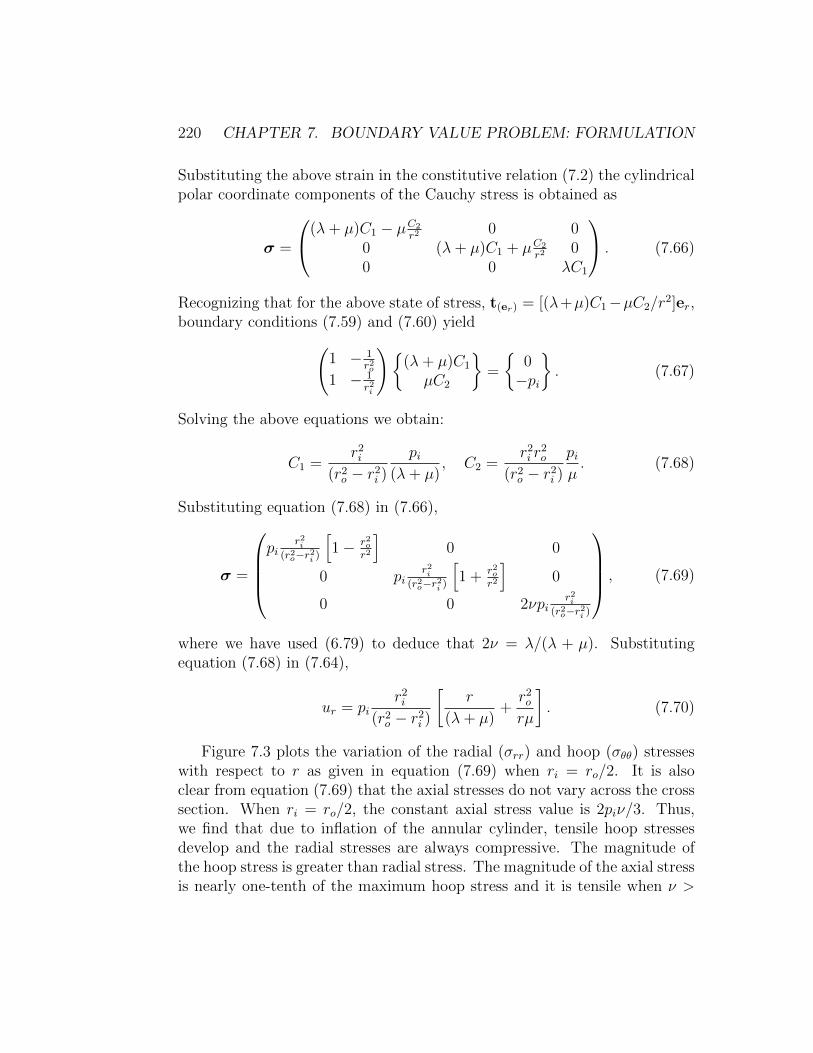
220 CHAPTER 7. BOUNDARY VALUE PROBLEM: FORMULATION
Substituting the above strain in the constitutive relation (7.2) the cylindricalpolar coordinate components of the Cauchy stress is obtained as
σ =
(λ+ µ)C1 − µC2
r20 0
0 (λ+ µ)C1 + µC2
r20
0 0 λC1
. (7.66)
Recognizing that for the above state of stress, t(er) = [(λ+µ)C1−µC2/r2]er,
boundary conditions (7.59) and (7.60) yield(1 − 1
r2o
1 − 1r2i
)(λ+ µ)C1
µC2
=
0−pi
. (7.67)
Solving the above equations we obtain:
C1 =r2i
(r2o − r2
i )
pi(λ+ µ)
, C2 =r2i r
2o
(r2o − r2
i )
piµ. (7.68)
Substituting equation (7.68) in (7.66),
σ =
pi
r2i(r2o−r2i )
[1− r2o
r2
]0 0
0 pir2i
(r2o−r2i )
[1 + r2o
r2
]0
0 0 2νpir2i
(r2o−r2i )
, (7.69)
where we have used (6.79) to deduce that 2ν = λ/(λ + µ). Substitutingequation (7.68) in (7.64),
ur = pir2i
(r2o − r2
i )
[r
(λ+ µ)+r2o
rµ
]. (7.70)
Figure 7.3 plots the variation of the radial (σrr) and hoop (σθθ) stresseswith respect to r as given in equation (7.69) when ri = ro/2. It is alsoclear from equation (7.69) that the axial stresses do not vary across the crosssection. When ri = ro/2, the constant axial stress value is 2piν/3. Thus,we find that due to inflation of the annular cylinder, tensile hoop stressesdevelop and the radial stresses are always compressive. The magnitude ofthe hoop stress is greater than radial stress. The magnitude of the axial stressis nearly one-tenth of the maximum hoop stress and it is tensile when ν >
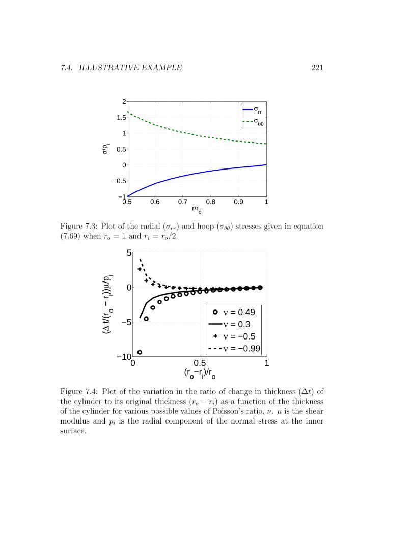
7.4. ILLUSTRATIVE EXAMPLE 221
0.5 0.6 0.7 0.8 0.9 1−1
−0.5
0
0.5
1
1.5
2
r/ro
σ/p i
σrr
σθθ
Figure 7.3: Plot of the radial (σrr) and hoop (σθθ) stresses given in equation(7.69) when ro = 1 and ri = ro/2.
0 0.5 1−10
−5
0
5
(ro−r
i)/r
o
(Δ t/
(ro −
ri))
μ/p i
ν = 0.49ν = 0.3ν = −0.5ν = −0.99
Figure 7.4: Plot of the variation in the ratio of change in thickness (∆t) ofthe cylinder to its original thickness (ro − ri) as a function of the thicknessof the cylinder for various possible values of Poisson’s ratio, ν. µ is the shearmodulus and pi is the radial component of the normal stress at the innersurface.

222 CHAPTER 7. BOUNDARY VALUE PROBLEM: FORMULATION
0 and compressive when ν < 0 and is zero when ν = 0. Next, we physicallyexplain this variation of the axial stresses with the Poisson’s ratio. The hoopstresses by virtue of being tensile in nature will cause a reduction in the axiallength due to Poisson’s effect3 if the Poisson’s ratio, ν > 0 and increase inlength if ν < 0 and no change if ν = 0. Similarly, the radial stress beingcompressive in nature will cause an increase in the axial length when ν >0, decrease in axial length when ν < 0 and no change in axial length whenν = 0. However, the actual change in axial length would be a sum of boththe change in length due to hoop and radial stress. Since, the hoop stressis more than the radial stress, if no axial force is applied, the axial lengthwould reduce when ν > 0, will not change when ν = 0 and will increasewhen ν < 0. Thus, if the length is to remain unchanged, a tensile axialforce has to be applied to counter the reduction in length when ν > 0 and acompressive axial force when ν < 0 and no axial force is required when ν =0. It can be seen from the expression for axial stress in equation (7.69) thatthe expression for the axial stresses is consistent with the expectation thatit be positive when ν > 0, negative when ν < 0 and zero when ν = 0.
Now, we study the changes that occur to the thickness of the annularcylinder. Towards this, the ratio of change in thickness of the cylinder, ∆tto its original thickness is obtained as
∆t
t=ur(ro)− ur(ri)
ro − ri=piµ
roro − ri
r2i
(r2o − r2
i )
1− ro
ri+
[1− ri
ro
]1− 2ν
(1− ν)
,
(7.71)where we have used (6.80) to write Lame constants in terms of the Poisson’sratio, ν and Young’s modulus E. Figure 7.4 plots the variation in the ratioof change in thickness of the cylinder to its original thickness as a function ofthe thickness of the cylinder for various possible values of Poisson’s ratio for agiven radial component of the normal stress at the inner surface, pi. It can beseen from the figure that while the thickness decreases when ν ≥ 0, thicknessincreases when ν < 0 for thickness less than a critical value. By virtue ofthe radial component of the normal stress being compressive in nature onewould expect a reduction in the thickness of the cylinder. However, the hoopstress being in tension, due to Poisson’s effect there would be reduction inthickness when ν > 0 and an increase when ν < 0. The actual change in thethickness is the sum of both the reduction due to radial stress and alteration
3Line elements on a plane whose normal coincides with the applied tensile stress shortenif ν > 0 and elongate if ν < 0. This effect is called as the Poisson’s effect.

7.4. ILLUSTRATIVE EXAMPLE 223
y
y
x
Figure 7.5: Schematic of pressurized hole in an infinite medium
due to hoop stress. Hence, the thickness decreases when ν ≥ 0 and increaseswhen ν < 0 for thickness less than a critical value.
Finally, we would like to show that due to inflation the inner as wellas outer radius of the cylinder increases. Noting that the deformed innerradius of the cylinder is ri + ur(ri) and that of the deformed outer radius isro + ur(ro), for these radius to increase we need to show that ur(ri) > 0 andur(ro) > 0. Towards this, using equation (7.70) and (6.80) we obtain,
ur(r) = rpiµ
r2i
(r2o − r2
i )
[(1− 2ν)
(1− ν)+r2o
r2
]. (7.72)
Recollecting from table 6.1, that the physically possible values for the Pois-son’s ratio is: −1 < ν ≤ 0.5, it is straightforward to see that (1−2ν)/(1−ν)≥ 0 for these possible range of values for ν. Also, it can be seen from table6.1 that µ > 0. Further, by definition ro > ri and pi > 0. Therefore, ur(r)> 0 for any r, since each term in the expression for ur is positive. Hence,in particular ur(ri) > 0 and ur(ro) > 0 and hence the radius of the cylinderincreases due to inflation, as one would expect.

224 CHAPTER 7. BOUNDARY VALUE PROBLEM: FORMULATION
Pressurized hole in an infinite medium
As a limiting case of the above solution, we would like to study the problemof a hole subjected to uniform radial component of the normal stress in aninfinite medium as shown in figure 7.5. We continue to use cylindrical polarcoordinates. Therefore the body in the reference configuration is assumed tooccupy the region of the Euclidean point space defined by B = (r, θ, z)|ri ≤r < ∞, 0 ≤ θ ≤ 2π,−∞ < z < ∞. The boundary conditions for thisproblem is essentially same as that in the inflation of an annular cylinder,except that now ro tends to ∞. For completeness the boundary conditionsfor the present problem is:
t(er)(∞, θ, z) = o, (7.73)
t(er)(ri, θ, z) = −pier, (7.74)
uz(r, θ,±∞) = 0. (7.75)
Hence, tending ro to ∞, in equations (7.69) and (7.70) we obtain the stressand displacement field for the present problem as,
σ =
−pi r2i
r20 0
0 pir2ir2
00 0 0
, (7.76)
ur =piµ
r2i
r. (7.77)
Thus, we find that both the stress and the displacement tend to zero as rtends to ∞. This means that the effect of pressurized hole is not felt at adistance far away from the hole.
Having studied the problem of pressurized hole, in the following sectionwe shall study the influence of the hole to uniaxial tensile load applied to theinfinite medium with the hole.
7.4.2 Uniaxial tensile loading of a plate with a hole
In the second boundary value problem that we study, the body is an infinitemedium with a circular stress free hole subjected to a far field tension alongthe x−direction as shown in the figure 7.6. We envisage to solve this bound-ary value problem using the stress formulation. In particular we assume

7.4. ILLUSTRATIVE EXAMPLE 225
x
y
a
Figure 7.6: Stress free hole in an infinite medium subjected to a uniform farfield tension along x−direction
plane stress state and the body to be two dimensional and use cylindricalpolar coordinates to study this problem. Thus, the body in the reference con-figuration is assumed to occupy a region in the Euclidean point space definedby B = (r, θ)|a ≤ r <∞, 0 ≤ θ ≤ 2π, where a is a constant characterizingthe size of the hole in the infinite medium. The boundary conditions that isof interest are
t(er)(a, θ) = o, (7.78)
t(cos(θ)er−sin(θ)eθ)(∞, θ) = σa [cos(θ)er − sin(θ)eθ] , (7.79)
t(sin(θ)er+cos(θ)eθ)(∞, θ) = o, (7.80)
This boundary condition needs some explanation. The boundary condition(7.78) tells that the boundary of the hole is traction free i.e.
σrr(a, θ) = 0, (7.81)
σrθ(a, θ) = 0. (7.82)
The second boundary condition (7.79) tells that the traction far away fromthe center of the hole, on a surface whose normal coincides with ex is σaex.Similarly, boundary condition (7.80) tells that a surface whose normal coin-cides with ey and is far away from the hole is traction free. In the equations(7.79) and (7.80), we have represented Cartesian basis ex and ey in cylindrical

226 CHAPTER 7. BOUNDARY VALUE PROBLEM: FORMULATION
polar coordinate basis. From equations (7.79) and (7.80) we obtain,
cos(θ) − sin(θ) 0
0 cos(θ) − sin(θ)sin(θ) cos(θ) 0
0 sin(θ) cos(θ)
σ∗rrσ∗rθσ∗θθ
=
σa cos(θ)−σa sin(θ)
00
, (7.83)
where σ∗ij represents the value of the stress at (∞, θ). Of the four equationsonly 3 are independent. Picking any three equations and solving for thecylindrical polar components of the stress, we obtain
σ∗rr = σrr(∞, θ) = σa1 + cos(2θ)
2, (7.84)
σ∗rθ = σrθ(∞, θ) = −σasin(2θ)
2, (7.85)
σ∗θθ = σθθ(∞, θ) = σa1− cos(2θ)
2. (7.86)
Thus, the boundary conditions translate into five conditions on the com-ponents of the stress given by equations, (7.81), (7.82), (7.84), (7.85) and(7.86).
Based on the observation that the far field stresses are a function ofcos(2θ), we infer that the Airy’s stress function, φ also should contain cos(2θ)term. Then, since the solution at θ equal to 0 and 2π should be the same,the Airy’s stress function can depend on θ only through the trigonometricfunctions present in the general solution (7.57). We assume Airy’s stressfunction with only five constants from the general solution (7.57) as,
φ = a02 ln(r) + a03r2 +
[a21r
2 + a23r−2 + a24
]cos(2θ), (7.87)
and examine whether the prescribed boundary conditions can be met. Con-sideration that the stress at ∞ be finite required dropping of the termsr2 ln(r) and r4. The constant a01 does not enter the expressions for stressand hence indeterminate. So we assumed it to be zero. For the assumptionof Airy’s stress function (7.87), the cylindrical polar components of the stress
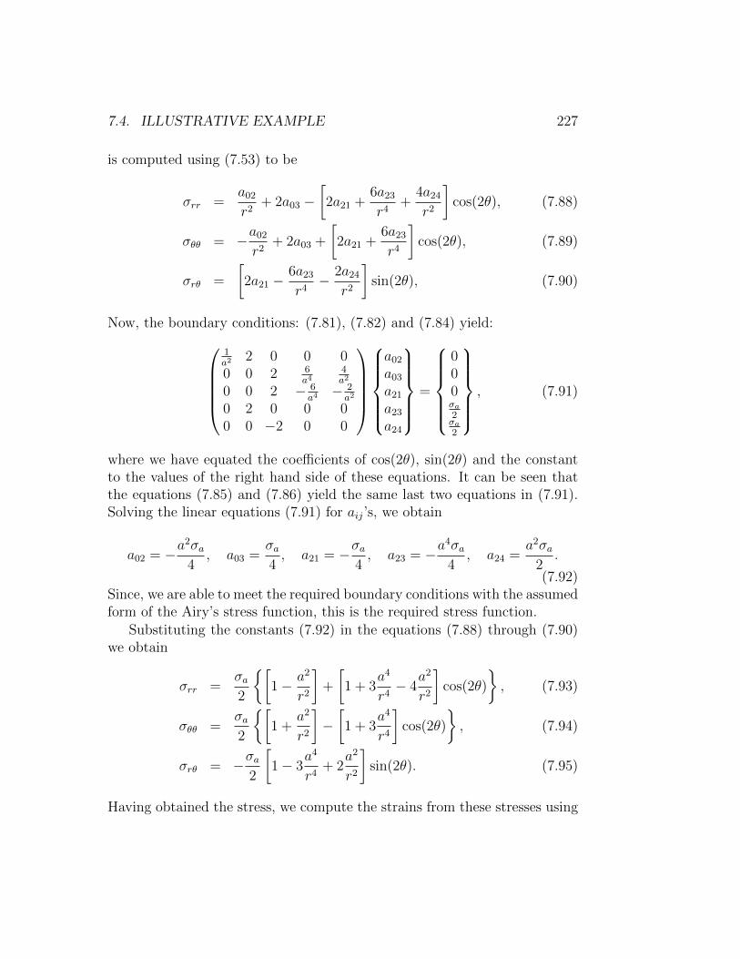
7.4. ILLUSTRATIVE EXAMPLE 227
is computed using (7.53) to be
σrr =a02
r2+ 2a03 −
[2a21 +
6a23
r4+
4a24
r2
]cos(2θ), (7.88)
σθθ = −a02
r2+ 2a03 +
[2a21 +
6a23
r4
]cos(2θ), (7.89)
σrθ =
[2a21 −
6a23
r4− 2a24
r2
]sin(2θ), (7.90)
Now, the boundary conditions: (7.81), (7.82) and (7.84) yield:1a2
2 0 0 00 0 2 6
a44a2
0 0 2 − 6a4− 2a2
0 2 0 0 00 0 −2 0 0
a02
a03
a21
a23
a24
=
000σa2σa2
, (7.91)
where we have equated the coefficients of cos(2θ), sin(2θ) and the constantto the values of the right hand side of these equations. It can be seen thatthe equations (7.85) and (7.86) yield the same last two equations in (7.91).Solving the linear equations (7.91) for aij’s, we obtain
a02 = −a2σa4
, a03 =σa4, a21 = −σa
4, a23 = −a
4σa4
, a24 =a2σa
2.
(7.92)Since, we are able to meet the required boundary conditions with the assumedform of the Airy’s stress function, this is the required stress function.
Substituting the constants (7.92) in the equations (7.88) through (7.90)we obtain
σrr =σa2
[1− a2
r2
]+
[1 + 3
a4
r4− 4
a2
r2
]cos(2θ)
, (7.93)
σθθ =σa2
[1 +
a2
r2
]−[1 + 3
a4
r4
]cos(2θ)
, (7.94)
σrθ = −σa2
[1− 3
a4
r4+ 2
a2
r2
]sin(2θ). (7.95)
Having obtained the stress, we compute the strains from these stresses using

228 CHAPTER 7. BOUNDARY VALUE PROBLEM: FORMULATION
the constitutive relation (7.54) as
εrr =∂ur∂r
=σa2
(1− ν)
E+
(1 + ν)
E
[−a
2
r2+
[1 + 3
a4
r4
]cos(2θ)
]− 4
E
a2
r2cos(2θ)
,
(7.96)
εθθ =1
r
∂uθ∂θ
+urr
=σa2
(1− ν)
E+
(1 + ν)
E
[a2
r2−[1 + 3
a4
r4
]cos(2θ)
]+
4ν
E
a2
r2cos(2θ)
,
(7.97)
εrθ =1
2
[1
r
∂ur∂θ
+∂uθ∂r− uθ
r
]= −(1 + ν)
E
σa2
[1− 3
a4
r4+ 2
a2
r2
]sin(2θ). (7.98)
Integrating equation (7.96) we obtain,
ur =σa2
(1− ν)
Er +
(1 + ν)
E
[a2
r+
[r − a4
r3
]cos(2θ)
]+
4
E
a2
rcos(2θ)
+df
dθ, (7.99)
where f = f(θ) is a function of θ. Substituting (7.99) in equation (7.97) andintegrating we find
uθ = −σa2
(1 + ν)
E
[r +
a4
r3
]+ 2
(1− ν)
E
a2
r
sin(2θ) + f(θ) + g(r), (7.100)
where g(r) is some function of r. Substituting equations (7.99) and (7.100)in equation (7.98) and simplifying we obtain
rdg
dr− g − f +
d2f
dθ2= 0. (7.101)
Since g is a function of only r and f only of θ, we require
rdg
dr− g = f − d2f
dθ2= C0, (7.102)

7.4. ILLUSTRATIVE EXAMPLE 229
where C0 is a constant. Solving the linear ordinary differential equations(7.102) we obtain
g = C1r − C0, f = C0 + C2 exp(θ) + C3 exp(−θ), (7.103)
where Ci’s are constants. To ensure that the tangential displacement of theray θ = 0 and θ = 2π to be the same and there be no rigid body displacementwe require that,
uθ(r, 0) = uθ(r, 2π) = 0. (7.104)
The condition (7.104) translates into requiring C1 = C2 = C3 = 0. Thus, thedisplacement field is computed to be,
ur =σa2
(1− ν)
Er +
(1 + ν)
E
[a2
r+
[r − a4
r3
]cos(2θ)
]+
4
E
a2
rcos(2θ)
,
(7.105)
uθ = −σa2
(1 + ν)
E
[r +
a4
r3
]+ 2
(1− ν)
E
a2
r
sin(2θ). (7.106)
Thus, we have found the displacement and stress field and hence have solvedthis boundary value problem. We would like to find the maximum stress thatoccurs and its location for this boundary value problem.
First we begin with hoop stress, σθθ given in equation (7.94). Recollectingthat the extremum value of a function could occur either at the boundarypoints or at points where the derivative of the function goes to zero, theextremum hoop stress could occur at a radial location, r = a
√6 cos(2θ),
when cos(2θ) > 0 or at the boundary points, r = a and r tending to ∞. Infigure 7.7 we plot the hoop stress as a function of r for various values of θ. Asexpected, the function is monotonically decreasing function of r when cos(2θ)< 0 and therefore the maximum value occurs at r = a for this case. Whencos(2θ) > 0, the minimum occurs at r = a, then the maximum occurs whenr = a
√6 cos(2θ) and then the stress decreases and asymptotically reaches
the value of σa[1− cos(2θ)]/2. Therefore, at r = a an extremum of the hoopstress occurs. The circumferential variation of the hoop stress at r = a isgiven by σa[1− 2 cos(2θ)]. Hence, the maximum hoop stress occurs at r = aand θ = π/2 (or θ = 3π/2) and the value of the maximum hoop stress is 3σa.Thus, the stress concentration factor, defined as the ratio of the maximumstress in the structure to the far field stress is 3 (= σmaxθθ /σa).
Next, we study the circumferential shearing stress, σrθ given in equation(7.95). The extremum value of this stress occurs at a radial location r = a
√3
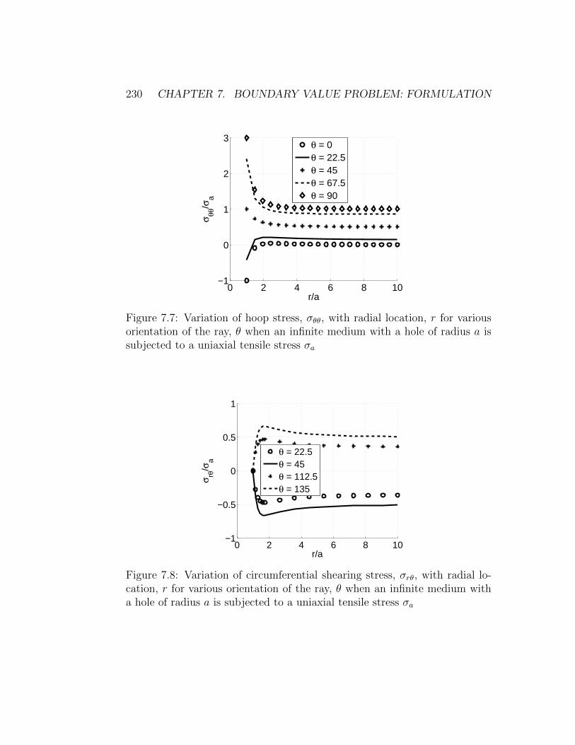
230 CHAPTER 7. BOUNDARY VALUE PROBLEM: FORMULATION
0 2 4 6 8 10−1
0
1
2
3
r/a
σ θθ/σ
a
θ = 0θ = 22.5θ = 45θ = 67.5θ = 90
Figure 7.7: Variation of hoop stress, σθθ, with radial location, r for variousorientation of the ray, θ when an infinite medium with a hole of radius a issubjected to a uniaxial tensile stress σa
0 2 4 6 8 10−1
−0.5
0
0.5
1
r/a
σ rθ/σ
a
θ = 22.5θ = 45θ = 112.5θ = 135
Figure 7.8: Variation of circumferential shearing stress, σrθ, with radial lo-cation, r for various orientation of the ray, θ when an infinite medium witha hole of radius a is subjected to a uniaxial tensile stress σa

7.4. ILLUSTRATIVE EXAMPLE 231
0 2 4 6 8 100
0.2
0.4
0.6
0.8
1
r/a
σ rr/σ
a
θ = 0θ = 15θ = 45θ = 90
(a) When r varies between 1 and 10
1 1.5 2−0.2
0
0.2
0.4
0.6
r/a
σ rr/σ
a
θ = 0θ = 15θ = 45θ = 90
(b) When r varies between 1 and 2
Figure 7.9: Variation of radial stress, σrr, with radial location, r for variousorientation of the ray, θ when an infinite medium with a hole of radius a issubjected to a uniaxial tensile stress σa
and the value of the circumferential shearing stress at this radial location is−2σa sin(2θ)/3. At the boundary points the circumferential shearing stresstakes values 0 at r = a and −σa sin(2θ)/2. The variation of σrθ with the radiallocation, r and the orientation of the ray, θ is shown in figure 7.8. Thus, itcan be seen that the absolute maximum value of the stress, σrθ occurs at r= a√
3, θ = mπ/4, where m takes one of the values from the set 1, 3, 5, 7and this maximum value is 2σa/3.
Finally, we examine the radial stress, σrr given in equation (7.93). Anextremum value of this stress occurs at
rcrit = a√
6 cos(2θ)/[1 + 4 cos(2θ)] (7.107)
when4 0 ≤ θ ≤ π/6 or 2π/6 ≤ θ ≤ 4π/6 or 5π/6 ≤ θ ≤ 7π/6 or 8π/6 ≤θ ≤ 10π/6 or 11π/6 ≤ θ ≤ 2π. This extremum value of the radial stressis −σa11 cos(2θ)/9 + 1/9 + 5/[36 cos(2θ)]/2. At the boundary the radialstresses takes the value 0 at r = a and σa[1 + cos(2θ)]/2 as r tends to ∞.Figure 7.9 portrays the variation of the radial stress with radial location, rfor various orientations of the ray, θ. It can be seen from the figure thatfor certain orientations (say, θ = 90 degrees) the maximum value of theradial stress occurs at r = a
√6 cos(2θ)/[1 + 4 cos(2θ)] and for some other
4The restriction on θ is obtained by the requirement that√
6 cos(2θ)/[1 + 4 cos(2θ)] ≥1.

232 CHAPTER 7. BOUNDARY VALUE PROBLEM: FORMULATION
0 100 200 300 400−1
−0.5
0
0.5
1
θ (degrees)
σ rrextr
emum
/σa
r = rcrit
r = ∞
Figure 7.10: Variation of two extremum radial stress σrr at rcrit [given inequation (7.107)] and as r tends to ∞, with the orientation of the ray, θwhen an infinite medium with a hole of radius a is subjected to a uniaxialtensile stress σa
orientations (say, θ = 15 degrees) the maximum value occurs when r tendsto ∞. To understand this, in figure 7.10 we plot the two extremum radialstresses - one at r = rcrit and the other value that occurs when r tends to∞. It can be seen from the figure that when π/3 ≤ θ ≤ 2π/3 and 8π/3 ≤ θ≤ 10π/3 the maximum radial stress occurs at rcrit and for all other values ofθ it occurs as r tends to ∞. In any case the maximum value is always lessthan σa.
This concludes our illustration of the two techniques to solve boundaryvalue problems in this chapter. However, in the remaining chapters we shallsee employment of these techniques to solve more boundary value problemsof interest in engineering.
7.5 General results
In this section, we record two results that are useful while solving boundaryvalue problems. One result tells when one can expect an unique solution toa given boundary value problem. The other allows us to construct solutionsto complex boundary conditions from simple cases.

7.5. GENERAL RESULTS 233
7.5.1 Uniqueness of solution
Now, we are interested in showing that there could at most be one solutionthat could satisfy the prescribed displacement or mixed boundary conditions,in a given body made of a material that obeys Hooke’s law and in static equi-librium with no body forces acting on it. If traction boundary condition isspecified, we shall see that the stress is uniquely determined but the displace-ment is not for the bodies made of a material that obeys Hooke’s law and instatic equilibrium with no body forces acting on it.
Towards this, we consider a general setting with B being some regionoccupied by the body and ∂B the boundary of the body. Let us also assumethat displacement is prescribed over some part of the boundary ∂Bu andtraction specified on the remaining part of the boundary, ∂Bσ. Let (u1, σ1)and (u2, σ2) be the two distinct solutions to a given boundary value problem.Let us define
u = u1 − u2, σ = σ1 − σ2. (7.108)
By virtue of (u1,σ1) and (u2, σ2) satisfying the specified boundary condi-tions,
u(x) = o, for x ∈ ∂Bu, (7.109)
t(n)(x) = σn = o, for x ∈ ∂Bσ. (7.110)
First, we examine the term,
W = σ · grad(u) = σ · ε, (7.111)
here to obtain the last equality we have used (2.104) and the fact that theCauchy stress σ is a symmetric tensor. Since, we are interested in materialsthat obey isotropic Hooke’s law, we substitute for the stress from5
σ =
[K − 2
3G
]tr(ε)1 + 2Gε, (7.112)
in (7.111) to obtain
W = K[tr(ε)]2 + 2G
tr(ε2)− 1
3[tr(ε)]2
. (7.113)
5This equation is obtained by writing Lame constants in terms of bulk modulus, K andshear modulus, G and substituting in equation (7.2).

234 CHAPTER 7. BOUNDARY VALUE PROBLEM: FORMULATION
As recorded in table 6.1 G > 0 and K > 0. Further recognizing that irre-spective of the sign of the Cartesian components of the strain,
tr(ε2)− 1
3[tr(ε)]2
=1
3
[(εxx − εyy)2 + (εyy − εzz)2 + (εzz − εxx)2
]+ 2ε2xy + 2ε2yz + 2ε2xz > 0,
(7.114)
on assuming that ε 6= 0. Thus, since each term in equation (7.113) is positivewe infer that
W > 0, (7.115)
as long as ε 6= 0.Next, we want to express∫
BWdv =
∫Bσ · grad(u)dv, (7.116)
in terms of the boundary conditions alone. Towards this, using the result inequation (2.219) we write
div(σu) = div(σ) · u + σ · grad(u). (7.117)
Since the body is in static equilibrium and has no body forces acting on it,from equation (7.6) div(σ) = o. Using div(σ) = o in equation (7.117) andsubstituting the result in (7.116) we get∫
BWdv =
∫Bdiv(σu)dv =
∫∂B
u · σtnda, (7.118)
where to obtain the last equality we have used the result (2.267). Substitutingthe conditions (7.109) and (7.110) on the displacement and stress, in (7.118)that ∫
BWdv = 0. (7.119)
Since, from equation (7.115) the integrand in the equation (7.119) is positiveand W = 0 only if ε = 0, it follows that ε = 0 everywhere in the body.Then, it is straight forward to see that σ = 0, everywhere in the body. Itcan then be shown that, we do this next for a special case, the conditions

7.5. GENERAL RESULTS 235
ε = 0 everywhere in the body and (7.109) imply u = o everywhere in thebody.
Integrating the first order differential equations on the Cartesian compo-nents of the displacement field when ε = 0, we obtain
u = (K1y+K2z+K4)ex+(−K1x+K3z+K5)ey−(K2x+K3y−K6)ez, (7.120)
whereKi’s are constants. Knowing the displacement of 3 points, say (x1, y1, z1),(x2, y2, z2) and (x3, y3, z3), that are not collinear to be zero, the constants Ki’scould be uniquely determined by solving the following system of equations:y1 z1 1
y2 z2 1y3 z3 1
K1
K2
K4
=
000
,
−x1 z1 1−x2 z2 1−x3 z3 1
K1
K3
K5
=
000
,
−x1 −y1 1−x2 −y2 1−x3 −y3 1
K2
K3
K6
=
000
. (7.121)
As long as the three points are not collinear, it can be seen that the above setof equations are independent and hence, Ki = 0. However, if the displacementis not known at 3 points, as in the case of traction boundary condition beingspecified, the displacement field cannot be uniquely determined.
Hence, we conclude that the solution to the boundary value probleminvolving a body in static equilibrium, under the absence of body forces andmade of a material that obeys isotropic Hooke’s law is unique except in caseswhere only traction boundary condition is specified. As a consequence ofthis theorem, if a solution has been found for a given boundary conditions itis the solution for a body in static equilibrium, under the absence of bodyforces and made of a material that obeys isotropic Hooke’s law.
7.5.2 Principle of superposition
This principle states that For a given body made up of a material thatobeys isotropic Hooke’s law, in static equilibrium and whose magnitude ofdisplacement is small, if u(1),σ(1) is a solution to the prescribed body
forces, b(1) and boundary conditions, u(1)b , t
(1)(n) and u(2),σ(2) is a solution
to the prescribed body forces, b(2) and boundary conditions, u(2)b , t
(2)(n) then
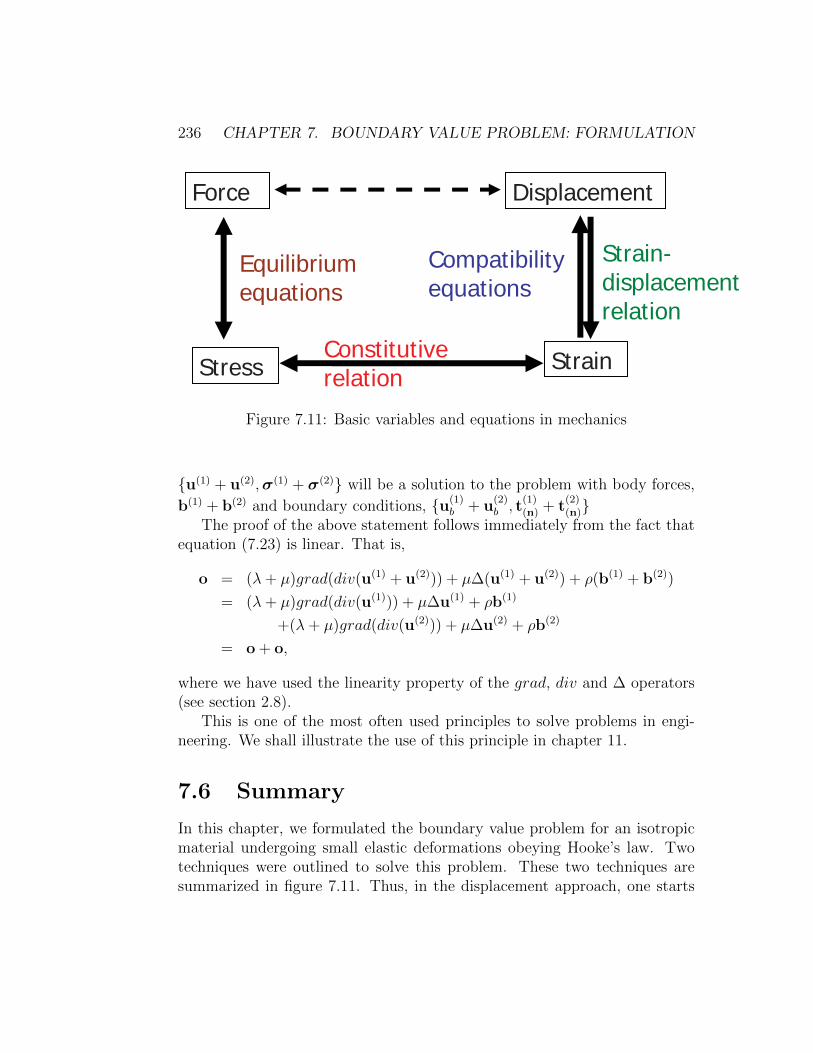
236 CHAPTER 7. BOUNDARY VALUE PROBLEM: FORMULATION
Force Displacement
Stress StrainConstitutiverelation
Strain-displacementrelation
Equilibrium e uations
Compatibilityequationsq
Figure 7.11: Basic variables and equations in mechanics
u(1) + u(2),σ(1) + σ(2) will be a solution to the problem with body forces,
b(1) + b(2) and boundary conditions, u(1)b + u
(2)b , t
(1)(n) + t
(2)(n)
The proof of the above statement follows immediately from the fact thatequation (7.23) is linear. That is,
o = (λ+ µ)grad(div(u(1) + u(2))) + µ∆(u(1) + u(2)) + ρ(b(1) + b(2))
= (λ+ µ)grad(div(u(1))) + µ∆u(1) + ρb(1)
+(λ+ µ)grad(div(u(2))) + µ∆u(2) + ρb(2)
= o + o,
where we have used the linearity property of the grad, div and ∆ operators(see section 2.8).
This is one of the most often used principles to solve problems in engi-neering. We shall illustrate the use of this principle in chapter 11.
7.6 Summary
In this chapter, we formulated the boundary value problem for an isotropicmaterial undergoing small elastic deformations obeying Hooke’s law. Twotechniques were outlined to solve this problem. These two techniques aresummarized in figure 7.11. Thus, in the displacement approach, one starts

7.7. SELF-EVALUATION 237
Figure 7.12: An annular cylinder pressurized from outside. (Figure for Prob-lem 1)
with the displacement use the strain displacement relation to compute thestrain and then the constitutive relation to find the stress and finally use theequilibrium equations to get the governing equation that the displacementfield has to satisfy along with the prescribed boundary conditions. In thestress approach, stress field is assumed in terms of a potential, such thatequilibrium equations hold, then the strain is computed using the constitu-tive relation. In order to be able to obtain a smooth displacement field usingthis strain field, it is required that the stress potential satisfy the compat-ibility conditions along with the prescribed boundary conditions. We thenillustrated these techniques by solving two boundary value problems, that ofinflation of an annular cylinder and that of a plate with a hole subjected touniaxial tension far away from the hole.
7.7 Self-Evaluation
1. A body in the form of an annular cylinder is pressurized from outside asshown in figure 7.12. Obtain the stress and displacement field for thisboundary value problem and show that the developed hoop stresses arecompressive in nature and that the thickness of the annular cylinderincreases due to the applied external pressure. Assume that the bodyis homogeneous and is made of a material that obeys isotropic Hooke’s

238 CHAPTER 7. BOUNDARY VALUE PROBLEM: FORMULATION
x
y
a
x
y
a
Figure 7.13: Stress free hole in an infinite medium subjected to equal biaxialloading. (Figure for Problem 2)
law.
2. Using the solution obtained in problem 1, study the problem of a stressfree hole in an infinite medium under equal biaxial loading at infinity,as shown in figure 7.13. Recognize that this solution can be obtainedby tending ro to ∞ in the solutions to problem 1. Then show that thehoop stresses developed at the boundary of the hole is twice the farfield equal biaxial stress applied.
3. The annular cylinder shown in figure 7.14 is pressurized from bothinside and outside. Assuming the cylinder to be homogeneous and madeof a material that obeys isotropic Hooke’s law with Young’s modulus,E = 200 GPa and Poisson’s ratio, ν = 0.3,
(a) Obtain the location and magnitude of the maximum and minimumhoop stress and radial stress.
(b) Obtain the maximum principal stress, its location and magnitude.
(c) Use thin cylinder approximation to obtain the hoop and radialstress. Use this to obtain the maximum principal stress.
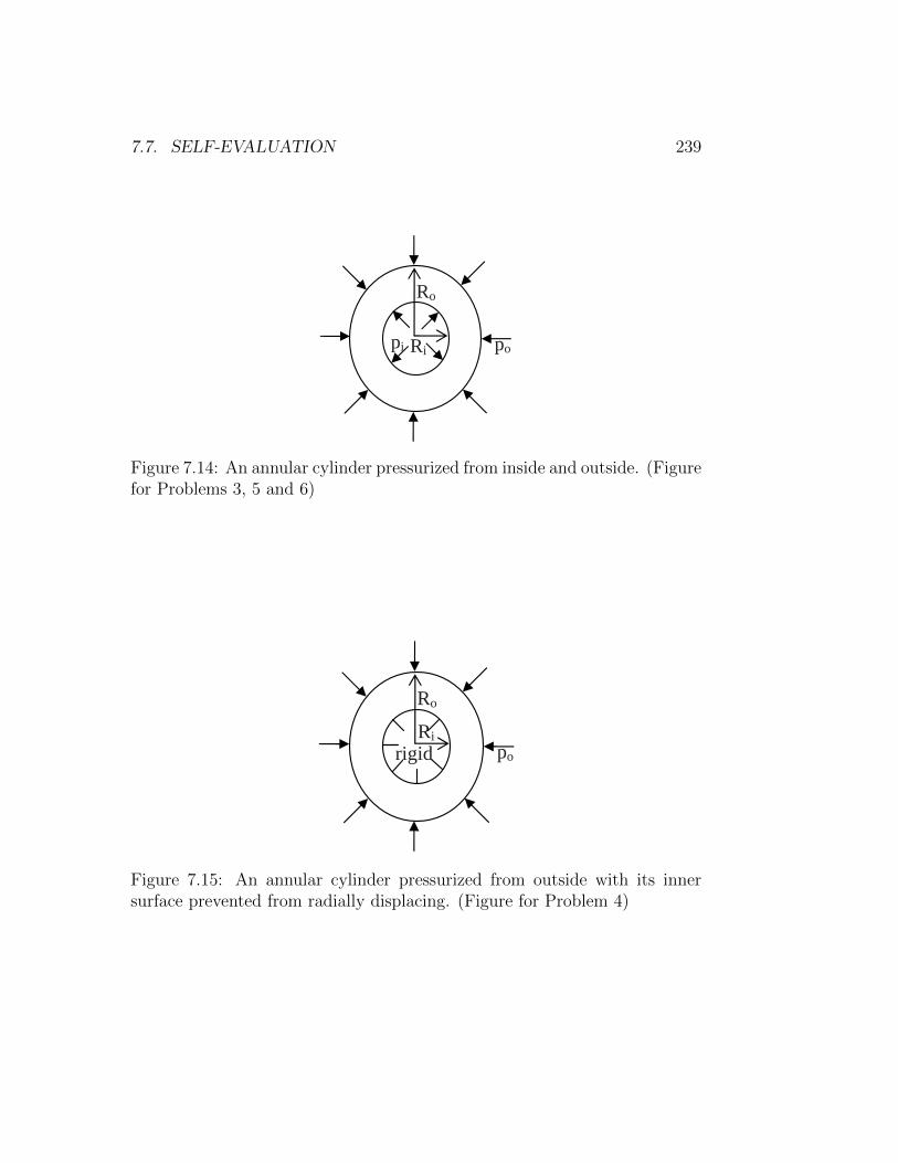
7.7. SELF-EVALUATION 239
pi po
Ro
Ri
Figure 7.14: An annular cylinder pressurized from inside and outside. (Figurefor Problems 3, 5 and 6)
Ro
Ririgid po
Figure 7.15: An annular cylinder pressurized from outside with its innersurface prevented from radially displacing. (Figure for Problem 4)

240 CHAPTER 7. BOUNDARY VALUE PROBLEM: FORMULATION
(d) Plot the ratio of the maximum principal stress obtained in part bto that in part c as a function of (1−Ri/Ro)−1 for Ri/Ro = 0.05to 0.99. Plot the same for (pi, po) = (1, 0), (0, 1), (1, 0.5), (0.5, 1).Using the above plots verify the reasonableness of the followingclassification: d/t < 20 thick cylinder, d/t > 40 thin cylinder,where d is the mean diameter of the cylinder and t is its thickness.
4. Assuming the annular cylinder shown in figure 7.15, to be homogeneousand made of a material that obeys isotropic Hooke’s law with Young’smodulus, E = 200 GPa and Poisson’s ratio, ν = 0.3 repeat parts (a)and (b) in problem 3. Here the inner boundary is fixed, i.e., ur(ri, θ, z)= 0. Find the hoop stress and radial stress as Ri/Ro tends to 0 andcomment on the significance of this limit.
5. Now assume the annular cylinder shown in figure 7.14 is inhomogeneousand is composed of two annular cylinders made of aluminium and steelrespectively. Solve parts (a) to (d) in problem 3 assuming
(a) Aluminium cylinder occupies the region B = (r, θ, z)|Ri ≤ r ≤(Ri + Ro)/2, 0 ≤ θ ≤ 2π, 0 ≤ z ≤ H and steel cylinder occupiesthe region B = (r, θ, z)|(Ri + Ro)/2 ≤ r ≤ Ro, 0 ≤ θ ≤ 2π, 0 ≤z ≤ H.
(b) Steel cylinder occupies the region B = (r, θ, z)|Ri ≤ r ≤ (Ri +Ro)/2, 0 ≤ θ ≤ 2π, 0 ≤ z ≤ H and aluminium cylinder occupiesthe region B = (r, θ, z)|(Ri + Ro)/2 ≤ r ≤ Ro, 0 ≤ θ ≤ 2π, 0 ≤z ≤ H.
Take Young’s modulus of steel and aluminium to be Esteel = 200 GPaand Ealuminium = 70 GPa respectively and Poisson’s ratio of these ma-terials to be νsteel = 0.3 and νaluminium = 0.27.
6. Assume that an aluminium annular cylinder occupying the region B= (r, θ, z)|Ri ≤ r ≤ (δ + (Ri + Ro)/2), 0 ≤ θ ≤ 2π, 0 ≤ z ≤ H inthe stress free state is shrunk and fitted into a steel annular cylinderoccupying the region B = (r, θ, z)|(Ri + Ro)/2 ≤ r ≤ Ro, 0 ≤ θ ≤2π, 0 ≤ z ≤ H in the stress free state. Then this composite shrinkfitted cylinder is pressurized as shown in figure 7.14. For this case solveparts (a) to (d) in problem 3. Assume δ = 0.0001Ro. Take Young’smodulus of steel and aluminium to be Esteel = 200 GPa and Ealuminium

7.7. SELF-EVALUATION 241
= 70 GPa respectively and Poisson’s ratio of these materials to be νsteel= 0.3 and νaluminium = 0.27.

242 CHAPTER 7. BOUNDARY VALUE PROBLEM: FORMULATION
Chapter 8
Bending of Prismatic StraightBeams
8.1 Overview
In this chapter, we formulate and study the bending of straight and prismaticbeams. First we study the bending of these beams when the loading is inthe plane of symmetry of the beams cross section. Here we derive again thestrength of materials solution and compare it with the solution obtained fromtwo dimensional elasticity formulation for two loading cases, namely purebending of a beam and uniform loading of a simply supported beam. Then,we study the bending of beams when the loading does not pass through theplane of symmetry. We do this by assuming the loading causes only bendingand no torsion. We will then show that for this to happen the load should beapplied at a point called the shear center of the cross-section. We concludeby presenting a method to compute this shear center.
Before proceeding further, let us begin by understanding what a beam is.A beam is a structural member whose length along one direction, called thelongitudinal axis, is larger than its dimensions on the plane perpendicular toit and is subjected to only transverse loads (i.e., the loads acting perpendic-ular to the longitudinal axis). A typical beam with rectangular cross sectionis shown in figure 8.1. Thus, this beam occupies the points in the Euclideanpoint space defined by B = (x, y, z)| − l ≤ x ≤ l,−c ≤ y ≤ c,−b ≤ z ≤ bwhere l, c and b are constants, such that l > c ≥ b with l/c typically in therange 10 to 20.
243
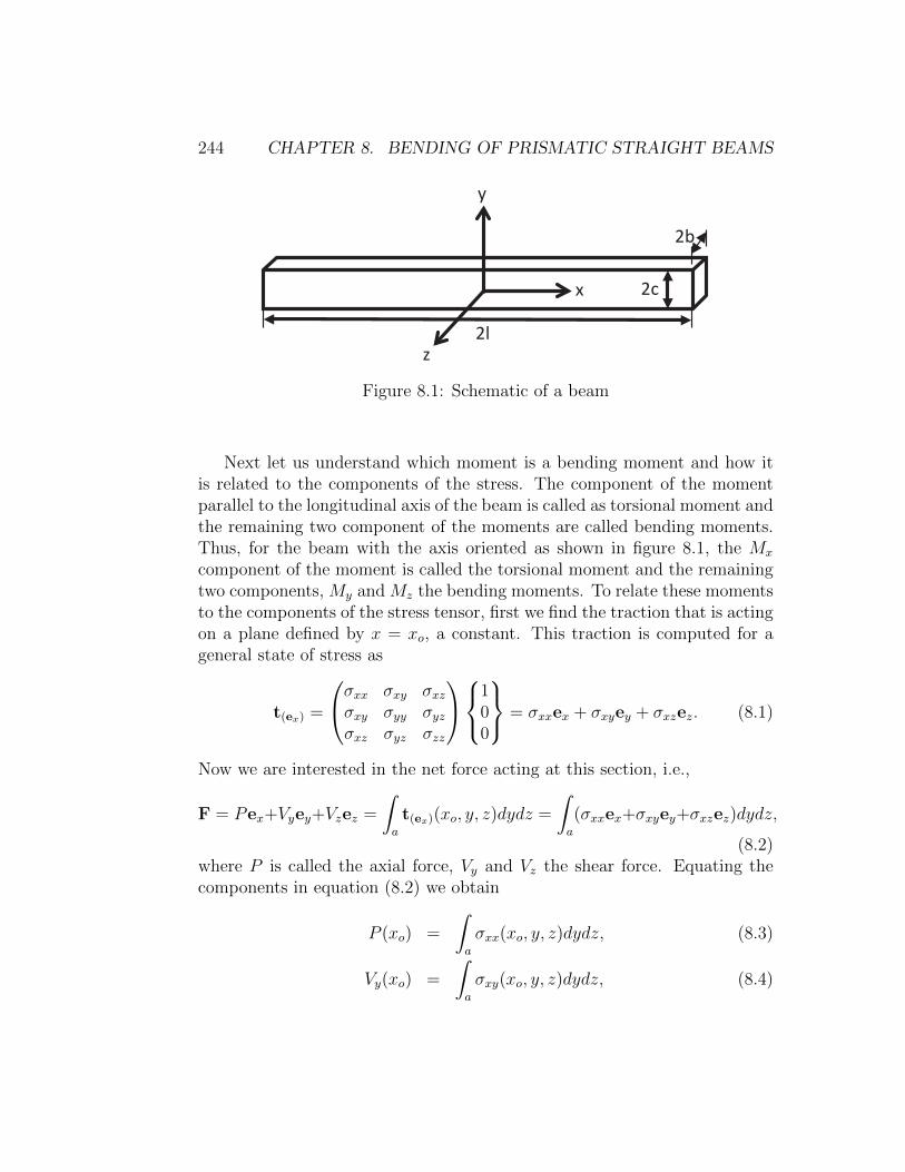
244 CHAPTER 8. BENDING OF PRISMATIC STRAIGHT BEAMS
x
y
z
2b
2c
2l
Figure 8.1: Schematic of a beam
Next let us understand which moment is a bending moment and how itis related to the components of the stress. The component of the momentparallel to the longitudinal axis of the beam is called as torsional moment andthe remaining two component of the moments are called bending moments.Thus, for the beam with the axis oriented as shown in figure 8.1, the Mx
component of the moment is called the torsional moment and the remainingtwo components, My and Mz the bending moments. To relate these momentsto the components of the stress tensor, first we find the traction that is actingon a plane defined by x = xo, a constant. This traction is computed for ageneral state of stress as
t(ex) =
σxx σxy σxzσxy σyy σyzσxz σyz σzz
100
= σxxex + σxyey + σxzez. (8.1)
Now we are interested in the net force acting at this section, i.e.,
F = Pex+Vyey+Vzez =
∫a
t(ex)(xo, y, z)dydz =
∫a
(σxxex+σxyey+σxzez)dydz,
(8.2)where P is called the axial force, Vy and Vz the shear force. Equating thecomponents in equation (8.2) we obtain
P (xo) =
∫a
σxx(xo, y, z)dydz, (8.3)
Vy(xo) =
∫a
σxy(xo, y, z)dydz, (8.4)

8.1. OVERVIEW 245
Vz(xo) =
∫a
σxz(xo, y, z)dydz, (8.5)
where the axial force and the shear force could vary along the longitudinalaxis of the beam. Then, we are also interested in the net moment actingabout the point (xo, y, z) due to the traction t(ex), i.e.,
M =
∫a
(yey + zez) ∧ (σxxex + σxyey + σxzez)dydz
=
∫a
[(σxzy − σxyz)ex + σxxzey − σxxy] dydz. (8.6)
Thus, the torsional moment is given by
Mx(xo) =
∫a
(σxzy − σxyz)dydz, (8.7)
and the two bending moments by
My(xo) =
∫a
σxxzdydz, (8.8)
Mz(xo) = −∫a
σxxydydz. (8.9)
The two shear forces and bending moments are also called as the force resul-tants or the stress resultants in the analysis of beams. These stress resultantsvary only along the longitudinal axis of the beam.
Next we want to recast the static equilibrium equations in the absence ofbody forces, (7.6) in terms of the stress resultants. Towards this, we recordthe differential form of the equilibrium equations in Cartesian coordinates:
∂σxx∂x
+∂σxy∂y
+∂σxz∂z
= 0, (8.10)
∂σxy∂x
+∂σyy∂y
+∂σyz∂z
= 0, (8.11)
∂σxz∂x
+∂σyz∂y
+∂σzz∂z
= 0, (8.12)
Multiply equation (8.10) with y and integrate over the cross sectionalarea to obtain∫
a
[∂(yσxx)
∂x+
(∂(yσxy)
∂y− σxy
)+∂(yσxz)
∂z
]dydz = 0, (8.13)

246 CHAPTER 8. BENDING OF PRISMATIC STRAIGHT BEAMS
Recognizing that in the first term the integration is with respect to y and zbut the differentiation is with respect to another independent variable x, theorder can be interchanged to obtain
∂
∂x
(∫a
σxxydydz
)= −dMz
dx, (8.14)
where we have used equation (8.9). To evaluate the second term in equation(8.13) we appeal to the Green’s theorem (2.275) and find that∫
a
∂(yσxy)
∂ydydz =
∮c
yσxynyds = 0, (8.15)
The last equality is because there are no shear stresses applied on the outerlateral surfaces of the beam. For the same reason the last term in equation(8.13) also evaluates to be zero:∫
a
∂(yσxz)
∂zdydz =
∮c
yσxznzds = 0. (8.16)
It follows from equation (8.4) that the third term in equation (8.13) is Vy,i.e., ∫
a
σxydydz = Vy. (8.17)
Substituting equations (8.14) through (8.17) in (8.13) and simplifying weobtain
dMz
dx+ Vy = 0. (8.18)
On multiplying equation (8.10) with z and integrating over the crosssectional area we obtain∫
a
[∂(zσxx)
∂x+∂(zσxy)
∂y+
(∂(zσxz)
∂z− σxz
)]dydz = 0. (8.19)
Using the equations (8.8) and (8.5) and Green’s theorem and following thesame steps as above, it can be shown that equation (8.19) evaluates to re-quiring
dMy
dx− Vz = 0. (8.20)
8.1. OVERVIEW 247
Integrating equation (8.11) over the cross sectional area we obtain∫a
[∂σxy∂x
+∂σyy∂y
+∂σyz∂z
]dydz = 0. (8.21)
Using equation (8.4), the first term in equation (8.21) evaluates to∫a
∂σxy∂x
dydz =dVydx
, (8.22)
where by virtue of the differentiation and integration being on different in-dependent variables, we have changed their order. Appealing to Green’stheorem (2.275), the second term in the equation (8.21) evaluates to∫
a
∂σyy∂y
dydz =
∮c
σyynyds = qy, (8.23)
where qy is the transverse loading per unit length applied on the beam. Thelast term in equation (8.21) evaluates as∫
a
∂σyz∂z
dydz =
∮c
σyznzds = 0, (8.24)
wherein we have again appealed to Green’s theorem (2.276) and the fact thatno shear stresses are applied on the lateral surface of the beam. Substitutingequations (8.22) through (8.24) in equation (8.21) it simplifies to
dVydx
+ qy = 0. (8.25)
Integrating equation (8.12) over the cross sectional area we obtain∫a
[∂σxz∂x
+∂σyz∂y
+∂σzz∂z
]dydz = 0. (8.26)
Using the equation (8.5) and the Green’s theorem and following the proce-dure similar to that described above, it can be shown that equation (8.26)simplifies to
dVzdx
+ qz = 0, (8.27)
where
qz =
∮c
σzznzds. (8.28)
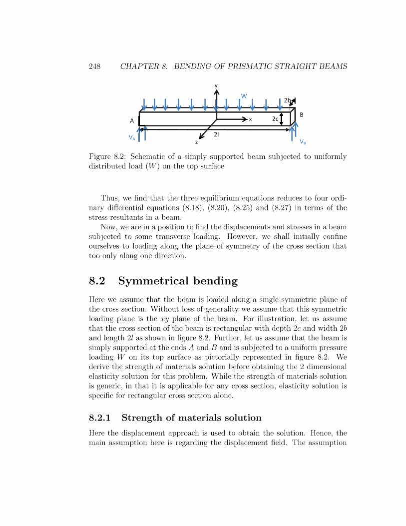
248 CHAPTER 8. BENDING OF PRISMATIC STRAIGHT BEAMS
x
y
z
2b
2c
2l VA
VB
W
A B
Figure 8.2: Schematic of a simply supported beam subjected to uniformlydistributed load (W ) on the top surface
Thus, we find that the three equilibrium equations reduces to four ordi-nary differential equations (8.18), (8.20), (8.25) and (8.27) in terms of thestress resultants in a beam.
Now, we are in a position to find the displacements and stresses in a beamsubjected to some transverse loading. However, we shall initially confineourselves to loading along the plane of symmetry of the cross section thattoo only along one direction.
8.2 Symmetrical bending
Here we assume that the beam is loaded along a single symmetric plane ofthe cross section. Without loss of generality we assume that this symmetricloading plane is the xy plane of the beam. For illustration, let us assumethat the cross section of the beam is rectangular with depth 2c and width 2band length 2l as shown in figure 8.2. Further, let us assume that the beam issimply supported at the ends A and B and is subjected to a uniform pressureloading W on its top surface as pictorially represented in figure 8.2. Wederive the strength of materials solution before obtaining the 2 dimensionalelasticity solution for this problem. While the strength of materials solutionis generic, in that it is applicable for any cross section, elasticity solution isspecific for rectangular cross section alone.
8.2.1 Strength of materials solution
Here the displacement approach is used to obtain the solution. Hence, themain assumption here is regarding the displacement field. The assumption
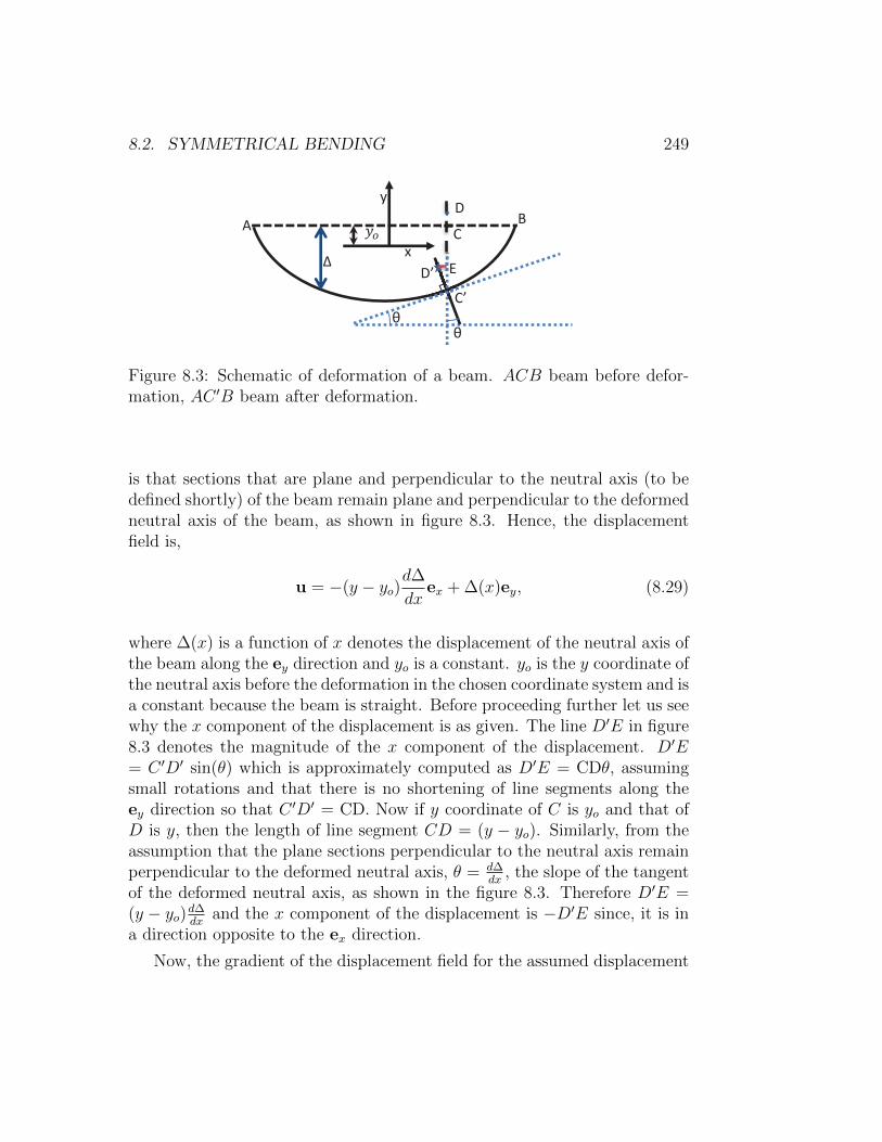
8.2. SYMMETRICAL BENDING 249
θ θ
x
B
Δ
A
y
C’
C
D
D’ E
Figure 8.3: Schematic of deformation of a beam. ACB beam before defor-mation, AC ′B beam after deformation.
is that sections that are plane and perpendicular to the neutral axis (to bedefined shortly) of the beam remain plane and perpendicular to the deformedneutral axis of the beam, as shown in figure 8.3. Hence, the displacementfield is,
u = −(y − yo)d∆
dxex + ∆(x)ey, (8.29)
where ∆(x) is a function of x denotes the displacement of the neutral axis ofthe beam along the ey direction and yo is a constant. yo is the y coordinate ofthe neutral axis before the deformation in the chosen coordinate system and isa constant because the beam is straight. Before proceeding further let us seewhy the x component of the displacement is as given. The line D′E in figure8.3 denotes the magnitude of the x component of the displacement. D′E= C ′D′ sin(θ) which is approximately computed as D′E = CDθ, assumingsmall rotations and that there is no shortening of line segments along theey direction so that C ′D′ = CD. Now if y coordinate of C is yo and that ofD is y, then the length of line segment CD = (y − yo). Similarly, from theassumption that the plane sections perpendicular to the neutral axis remainperpendicular to the deformed neutral axis, θ = d∆
dx, the slope of the tangent
of the deformed neutral axis, as shown in the figure 8.3. Therefore D′E =(y − yo)d∆
dxand the x component of the displacement is −D′E since, it is in
a direction opposite to the ex direction.
Now, the gradient of the displacement field for the assumed displacement
250 CHAPTER 8. BENDING OF PRISMATIC STRAIGHT BEAMS
(8.29) is
h =
−[y − yo]d2∆dx2
−d∆dx
0d∆dx
0 00 0 0
, (8.30)
and therefore the linearized strain is
ε =1
2[h + ht] =
−[y − yo]d2∆dx2
0 00 0 00 0 0
. (8.31)
Using the one dimensional constitutive relation, σ(n) = Eε(n), where σ(n) andε(n) are the normal stress and strain along the direction n, we obtain
σxx = −E[y − yo]d2∆
dx2, (8.32)
where we have equated the normal stress and strain along the ex direction.Substituting equation (8.32) in the equation (8.3) we obtain
P =
∫a
E[y − yo]d2∆
dx2da. (8.33)
Since, in a beam there would be no net applied axial load P = 0. Solvingequation (8.33) for yo under the assumption that no net axial load is applied,
yo =
∫aEyda∫aEda
. (8.34)
If the beam is also homogeneous then Young’s modulus, E is a constant andtherefore, yo = (
∫ayda)/(
∫ada), centroid of the cross section. Since, we have
assumed that there is no net applied axial load, i.e.,∫a
σxxda = 0, (8.35)
equation (8.9) can be written as,
Mz = −∫a
yσxxda = −∫a
yσxxda+
∫a
yoσxxda = −∫a
[y − yo]σxxda, (8.36)
8.2. SYMMETRICAL BENDING 251
where yo is a constant given in equation (8.34). Substituting equation (8.32)in equation (8.36) we obtain,
Mz =
∫a
[y − yo]2Ed2∆
dx2da =
d2∆
dx2
∫a
[y − yo]2Eda. (8.37)
If the cross section of the beam is homogeneous, the above equation can bewritten as,
Mz =d2∆
dx2E
∫a
[y − yo]2da =d2∆
dx2EIzz, (8.38)
where,
Izz =
∫a
[y − yo]2da, (8.39)
is the moment of inertia about the z axis.Combining equations (8.37) and (8.32) we obtain for inhomogeneous
beams
− σxxE(y − yo)
=d2∆
dx2=
Mz∫a[y − yo]2Eda
, (8.40)
where yo is as given in equation (8.34). Combining equations (8.38) and(8.32) we obtain for homogeneous beams
− σxx(y − yo)
= Ed2∆
dx2=Mz
Izz, (8.41)
where yo is the y coordinate of the centroid of the cross section which canbe taken as 0 without loss of generality provided the origin of the coordinatesystem used is located at the centroid of the cross section.
Next, we would like to define neutral axis. Neutral axis is defined as theline of intersection of the plane on which the bending stress is zero (y = yo)and the plane along which the resultant load acts.
Equations (8.40) and (8.41) relate the bending stresses and displacementto the bending moment in an inhomogeneous and homogeneous beam re-spectively and is called as the bending equation. While these equations aresufficient to find all the stresses in a beam subjected to a constant bendingmoment, one further needs to relate the shear stresses to the shear force thatarises when the beam is subjected to a bending moment that varies alongthe longitudinal axis of the beam. This we shall do next.
Consider a section of the beam, pqrs as shown in figure 8.4 when thebeam is subjected to a bending moment that varies along the longitudinal

252 CHAPTER 8. BENDING OF PRISMATIC STRAIGHT BEAMS
co
s r τ
N.A.
p q
Mz rVy
Δx
c
t
Figure 8.4: Schematic of stresses acting on a beam subjected to varyingbending moment
axis of the beam. For the force equilibrium of section pqrs, the shear stress,τ , as indicated in the figure 8.4 should be
τ(∆X)t =
∫a
[y − yo]
1
Izz
[Mz +
dMz
dx∆x
]− [y − yo]
Mz
Izz
da
=dMz
dx
∆X
Izz
∫a
[y − yo]da, (8.42)
where the integration is over the cross sectional area above the section ofinterest, i.e., the shaded area shown in figure 8.4 and t is the width of thecross section at the section of interest. Substituting equation (8.18) in (8.42)and simplifying we obtain,
τ = − VyIzzt
∫a
[y − yo]da. (8.43)
Having obtained the magnitude of this shear stress, next we discuss thedirection along which this acts. For thick walled sections with say, l/b < 20,as in the case of well proportioned rectangular beams, this shear stress is theσxy (and the complimentary σyx) component. For thin walled sections, thisshear stress would act tangential to the profile of the cross section as shownin the figure 8.5b and figure 8.5c. Thus it has both the σxy and σxz shearcomponents acting on these sections.
8.2.2 2D Elasticity solution
While the strength of material solution is generic in that it can be used forany type of loading and cross sections of any shape as long as it is loaded in

8.2. SYMMETRICAL BENDING 253
τ
(a) Thick walled rectangu-lar section.
τ τ
τ
τ τ (b) Thin walled I sec-tion.
τ
τ
τ τ
τ
τ
(c) Thin walled circular section.
Figure 8.5: Direction of the shear stresses acting on a cross section of a beamsubjected to varying bending moment
its plane of symmetry, 2D elasticity solution has to be developed for specificcross sections and loading scenarios. Consequently, we assume that the crosssection is rectangular in shape with width 2b and depth 2c. Thus, the bodyis assumed to occupy the region in the Euclidean point space defined by B= (x, y, z)| − l ≤ x ≤ l,−c ≤ y ≤ c,−b ≤ z ≤ b before the application ofthe load. Using the stress formulation introduced in chapter 7, we study theresponse of this body subjected to three types of load.
Pure bending of a simply supported beam
Consider the case of a straight beam subject to end moments as shown infigure 8.6. It can be seen from the figure that the top and bottom surfacesare free of traction, i.e.
t(ey)(x, c) = o, t(−ey)(x,−c) = o. (8.44)
The surfaces defined by x = ±l has traction on its face such that the netforce is zero but it results in a bending moment, Mz. Representing these

254 CHAPTER 8. BENDING OF PRISMATIC STRAIGHT BEAMS
y
x
M M
2c
2l
Figure 8.6: Beam subjected to end moments
conditions mathematically,∫a
t(ex)(l, y)dydz = o,
∫a
t(−ex)(−l, y)dydz = o,∫a
(yey + zez) ∧ t(ex)(l, y)dydz = Mez,∫a
(yey + zez) ∧ t(−ex)(−l, y)dydz = −Mez. (8.45)
Thus, the exact point wise loading on the ends is not considered and onlythe statically equivalent effect is modeled. Consequently, the boundary con-ditions on the ends of the beam have been relaxed, and only the staticallyequivalent condition will be satisfied. This fact leads to a solution that is notnecessarily valid at the ends of the beam and could result in more than onestress field satisfying the prescribed conditions.
Assuming the state of stress to be plane, such that
σ =
σxx σxy 0σxy σyy 00 0 0
, (8.46)
the boundary condition (8.44) translates into requiring,
σyy(x,±c) = 0, (8.47)
σxy(x,±c) = 0. (8.48)

8.2. SYMMETRICAL BENDING 255
For the assumed state of stress (8.46) the boundary condition (8.45) requires,∫ c
−c2bσxy(±l, y)dy = 0, (8.49)∫ b
−bzdz
∫ c
−cσxy(±l, y)dy = 0, (8.50)∫ c
−c2bσxx(±l, y)dy = 0, (8.51)∫ c
−c2bσxx(±l, y)ydy = −M. (8.52)
Recognize that condition (8.50) holds irrespective of what the variation ofthe shear stress σxy is.
As discussed in detail in chapter 7 (section 7.3.2), for stress formulation,we assume that the Cartesian components of stress are obtained from a po-tential, φ = φ(x, y), called the Airy’s stress function through
σxx =∂2φ
∂y2, σyy =
∂2φ
∂x2, σxy = − ∂2φ
∂x∂y. (8.53)
Then, we have to find the potential such that it satisfies the boundary con-ditions (8.47) through (8.52) and the bi-harmonic equation, ∆(∆(φ)) = 0.
We express φ as a power series:
φ(x, y) =∞∑m=0
∞∑n=0
Amnxmyn, (8.54)
where Amn are constant coefficients to be determined from the boundaryconditions and the requirement that it satisfy the bi-harmonic equation.
The choice of the stress function is based on the fact that a third orderAiry’s stress function will give rise to a linear stress field, and this linearboundary loading on the ends x = ±l, will satisfy the requirements (8.49)through (8.52). Based on this observation, we choose the Airy’s stress func-tion as
φ = A03y3 + A30x
3 + A21x2y + A12xy
2. (8.55)
Then, the stress field takes the form
σxx = 6A03y+2A12x, σyy = 6A30x+2A21y, σxy = 2[A12y+A21x]. (8.56)
256 CHAPTER 8. BENDING OF PRISMATIC STRAIGHT BEAMS
Substituting the above stress in boundary conditions (8.47) and (8.48) wefind that A30 = A21 = A12 = 0. Thus, the Airy’s stress function reduces to,
φ = A03y3, (8.57)
and the stress field becomes
σxx = 6A03y, σyy = σxy = 0. (8.58)
Substituting (8.60) in the boundary conditions (8.49) through (8.52), we findthat (8.49) through (8.51) are satisfied identically and (8.52) requires,
A03 = −1
8
M
c3b. (8.59)
It can be verified that the Airy’s stress function (8.57) satisfies the bi-harmonic equation trivially.
Substituting (8.59) in (8.58) we obtain,
σxx =3M
4c3by, σyy = σxy = 0. (8.60)
Using the 2 dimensional Hooke’s law (7.49), the strain field correspondingto the stress field (8.60) is computed to be
εxx =∂ux∂x
= − 3M
4Ec3by, (8.61)
εyy =∂uy∂y
= ν3M
4Ec3by, (8.62)
εxy =1
2
[∂ux∂y
+∂uy∂x
]= 0. (8.63)
Integrating (8.61) we obtain
ux = − 3M
4Ec3bxy + f(y), (8.64)
where f is an arbitrary function of y. Similarly, integrating (8.62) we obtain
uy =3Mν
8Ec3by2 + g(x), (8.65)
8.2. SYMMETRICAL BENDING 257
where g is an arbitrary function of x. Substituting equations (8.64) and(8.65) in equation (8.63) and simplifying we obtain
− 3M
4Ec3bx+
df
dy+dg
dx= 0. (8.66)
For equation (8.66) to hold,
df
dy= −C0,
dg
dx= C0 +
3M
4Ec3bx, (8.67)
where C0 is a constant. Integrating (8.67) we obtain
f(y) = −C0y + C1, g(x) = C0x+3M
8Ec3bx2 + C2, (8.68)
where C1 and C2 are integration constants. Substituting (8.68) in equations(8.64) and (8.65) we obtain
ux = − 3M
4Ec3bxy − C0y + C1, uy =
3M
8Ec3b[x2 + νy2] + C0x+ C2. (8.69)
The constants Ci’s are to be evaluated from displacement boundary con-ditions. Assuming the beam to be simply supported at the ends A and B,we require
uy(±l, 0) = 0, and ux(−l, 0) = 0, (8.70)
where we have assumed the left side support to be hinged (i.e., both the ver-tical and horizontal displacement is not possible) and the right side supportto be a roller (i.e. only vertical displacement is restrained). Substituting(8.69) in (8.70) we obtain
C0l + C2 = − 3Ml2
8Ec3b, (8.71)
−C0l + C2 = − 3Ml2
8Ec3b, (8.72)
C1 = 0. (8.73)
Solving the equations (8.71) and (8.72) for C0 and C2 we obtain
C0 = 0, C2 = − 3Ml2
8Ec3b. (8.74)

258 CHAPTER 8. BENDING OF PRISMATIC STRAIGHT BEAMS
Substituting, equations (8.73) and (8.74) in the equation (8.69) we obtainthe displacement field as,
u = − 3M
4Ec3bxyex +
3M
8Ec3b[x2 + νy2 − l2]ey. (8.75)
If the displacement boundary condition is different, then the requirement(8.70) will change and hence the displacement field.
We now wish to compare this elasticity solution with that obtained bystrength of materials approach. The bending equation (8.41), for rectangularcross section being studied and the constant moment case reduces to,
− σxxy
=3M
4c3b= E
d2∆
dx2, (8.76)
where we have used the fact that for a rectangular cross section of depth 2cand width 2b, Izz = 4c3b/3 and that yo = 0 as the origin is at the centroidof the cross section. Using the first equality in equation (8.76) we obtain thestress field as,
σxx = − 3M
4c3by, σyy = σxy = 0, (8.77)
Comparing equations (8.60) and (8.77) we find that the stress field is the samein both the approaches. Then, using the last equality in equation (8.76) weobtain,
∆ =3M
4c3b
x2
2+D1x+D2, (8.78)
where D1 and D2 are integration constants to be found from the displace-ment boundary condition (8.70). This simply supported boundary conditionrequires that ∆(±l) = 0, i.e.,
D1l +D2 = − 3M
4c3b
l2
2, (8.79)
−D1l +D2 = − 3M
4c3b
l2
2. (8.80)
Solving the above equations we obtain,
D1 = 0, D2 = − 3M
4c3b
l2
2. (8.81)
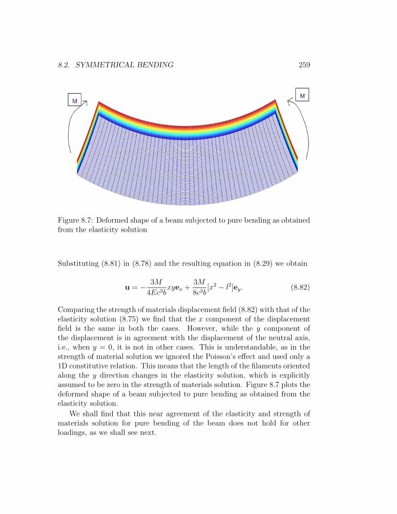
8.2. SYMMETRICAL BENDING 259
Figure 8.7: Deformed shape of a beam subjected to pure bending as obtainedfrom the elasticity solution
Substituting (8.81) in (8.78) and the resulting equation in (8.29) we obtain
u = − 3M
4Ec3bxyex +
3M
8c3b[x2 − l2]ey. (8.82)
Comparing the strength of materials displacement field (8.82) with that of theelasticity solution (8.75) we find that the x component of the displacementfield is the same in both the cases. However, while the y component ofthe displacement is in agreement with the displacement of the neutral axis,i.e., when y = 0, it is not in other cases. This is understandable, as in thestrength of material solution we ignored the Poisson’s effect and used only a1D constitutive relation. This means that the length of the filaments orientedalong the y direction changes in the elasticity solution, which is explicitlyassumed to be zero in the strength of materials solution. Figure 8.7 plots thedeformed shape of a beam subjected to pure bending as obtained from theelasticity solution.
We shall find that this near agreement of the elasticity and strength ofmaterials solution for pure bending of the beam does not hold for otherloadings, as we shall see next.

260 CHAPTER 8. BENDING OF PRISMATIC STRAIGHT BEAMS
y
x
2l
2c wlwl
w
Figure 8.8: Beam carrying uniformly transverse loading.
Simply supported beam subjected to uniformly distributed trans-verse loading
The next problem that we solve is that of a beam carrying a uniformlydistributed transverse loading w along its top surface,as shown in Figure 8.8.As before the traction boundary conditions for this problem are
t(ey)(x, c) = −w2b
ey, (8.83)
t(−ey)(x,−c) = o, (8.84)
∫ c
−c2bt(ex)(l, y)dy = wley, (8.85)∫ c
−c2bt(−ex)(−l, y)dy = wley, (8.86)
∫ c
−c2b(yey + zez) ∧ t(ex)(l, y)dy = o, (8.87)∫ c
−c2b(yey + zez) ∧ t(−ex)(−l, y)dy = o. (8.88)
8.2. SYMMETRICAL BENDING 261
While exact point wise conditions are specified on the top and bottom sur-faces, at the right and left surfaces the resultant horizontal axial force andmoment are set to zero and the resultant vertical shear force is specifiedsuch that it satisfies the overall equilibrium. As before assuming plane stressconditions, (8.46), the boundary conditions (8.83) through (8.88) evaluatesto,
σxy(x,±c) = 0, (8.89)
σyy(x,−c) = 0, (8.90)
σyy(x, c) = −w2b, (8.91)∫ c
−cσxx(±l, y)dy = 0, (8.92)∫ c
−cσxy(l, y)dy = wl, (8.93)∫ c
−cσxy(−l, y)dy = −wl, (8.94)∫ c
−cσxx(±l, y)ydy = 0. (8.95)
Thus, we have to chose Airy’s stress function such that conditions (8.89)through (8.95) holds along with the bi-harmonic equation.
Seeking Airy’s stress function in the form of the polynomial (8.54), wetry the following form,
φ = A20x2 + A21x
2y + A03y3 + A23x
2y3 + A05y5, (8.96)
where Aij’s are constants. For this polynomial to satisfy the bi-harmonicequation,
∂4φ
∂x4+ 2
∂4φ
∂x2∂y2+∂4φ
∂y4= 0, (8.97)
it is required that
A05 = −A23
5. (8.98)
For this assumed form for the Airy’s stress function (8.96), the stress field
262 CHAPTER 8. BENDING OF PRISMATIC STRAIGHT BEAMS
found using equation 8.53 is,
σxx = 6A03y + 6A23(x2y − 2
3y3), (8.99)
σyy = 2A20 + 2A21y + 2A23y3, (8.100)
σxy = −2A21x− 6A23xy2, (8.101)
where we have used (8.98).
Substituting equation (8.101) in the boundary condition (8.89) we obtain,
A21 + 3A23c2 = 0. (8.102)
Then, using equation (8.100) in the boundary conditions (8.90),(8.91) weobtain,
2A20 − 2A21c− 2A23c3 = 0, (8.103)
2A20 + 2A21c+ 2A23c3 = −w
2b. (8.104)
Solving the above three equations for the constants A20, A21 and A23, weobtain
A20 = −w8b, A21 = − 3w
16bc, A23 =
w
16bc3. (8.105)
Next, substituting equation (8.99) in the boundary condition (8.92) we findthat it holds for any choice of the remaining constant, A03. Similarly, whenthe constants, Aij are as given in (8.105), the shear stress (8.101) satisfies theboundary conditions (8.93) and (8.94). Thus, substituting equation (8.99) inthe boundary condition (8.95) we obtain
A03 = −A23(l2 − 2
5c2) = − w
16bc
[l2
c2− 2
5
]. (8.106)
Thus, the assumed form for the Airy’s stress function (8.96) with the appro-priate choice for the constants, satisfies the required boundary conditions andthe bi-harmonic equation and therefore is a solution to the given boundaryvalue problem.
Substituting the values for the constants from equations (8.105) and(8.106) in equations (8.99) through (8.101), the resulting stress field can

8.2. SYMMETRICAL BENDING 263
be written as,
σxx = − 3w
8bc
[l2
c2− 2
5
]y +
3w
8bc3
[x2y − 2
3y3
], (8.107)
σyy = −w4b
[1 +
3
2
y
c− 1
2
y3
c3
], (8.108)
σxy =3wx
8bc
[1− y2
c2
]. (8.109)
Having computed the stress fields, next we determine the displacementfield. As usual, we use the 2 dimensional constitutive relation (7.49) to obtainthe strain field as
εxx =∂ux∂x
=σxxE− νσyy
E
=w
4Eb
3y
2c3
[x2 − 2
3y2
]− 3y
2c
[l2
c2− 2
5
]+ ν
[1 +
3
2
y
c− 1
2
y3
c3
], (8.110)
εyy =∂uy∂y
=σyyE− νσxx
E
=w
4Eb
−[1 +
3
2
y
c− 1
2
y3
c3
]− 3yν
2c3
[x2 − 2
3y2
]+
3yν
2c
[l2
c2− 2
5
], (8.111)
εxy =1
2
[∂ux∂y
+∂uy∂x
]= σxy
(1 + ν)
E=
(1 + ν)
E
3wx
8bc
[1− y2
c2
]. (8.112)
Integrating (8.110) we obtain
ux =w
4Eb
yx
2c3
[x2 − 2y2 − 3l2 +
3
5c2
]+ νx
[1 +
3
2
y
c− 1
2
y3
c3
]+ f(y)
,
(8.113)
where f(y) is a yet to be determined function of y. Similarly integrating(8.111),
uy = − w
4Eb
y +
3
4
y2
c− 1
8
y4
c3+
3y2ν
4c3
[x2 − 1
3y2
]− 3y2ν
4c
[l2
c2− 2
5
]−g(x) , (8.114)

264 CHAPTER 8. BENDING OF PRISMATIC STRAIGHT BEAMS
where g(x) is a yet to be determined function of x.Substituting equations (8.113) and (8.114) in (8.112) and simplifying we
obtainx3
2c3− 27
10
x
c− 3ν
2
x
c− 3
2
l2x
c3+df
dy+dg
dx= 0. (8.115)
For equation (8.115) to hold,
df
dy= C0,
dg
dx= − x3
2c3+
27
10
x
c+
3ν
2
x
c+
3
2
l2x
c3+ C0, (8.116)
where C0 is a constant. Integrating the differential equation (8.115) we obtain
f(y) = C0y + C1, (8.117)
g(x) =x2
2c
[27
10+
3ν
2+
3l2
2c2
]− x4
8c3+ C0x+ C2, (8.118)
(8.119)
where C1 and C2 are constants to be determined from the displacementboundary condition. Assuming the beam to be simply supported at the endsA and B, we require
uy(±l, 0) = 0, and ux(−l, 0) = 0, (8.120)
where we have assumed the left side support to be hinged (i.e., both the ver-tical and horizontal displacement is not possible) and the right side supportto be a roller (i.e. only vertical displacement is restrained). Substituting(8.114) and (8.118) in (8.120a) we obtain
C0l + C2 =l4
8c3− l2
2c
[27
10+
3ν
2+
3l2
2c2
], (8.121)
−C0l + C2 =l4
8c3− l2
2c
[27
10+
3ν
2+
3l2
2c2
]. (8.122)
Solving equations (8.121) and (8.122) for C0 and C2,
C0 = 0, C2 =l4
8c3− l2
2c
[27
10+
3ν
2+
3l2
2c2
]. (8.123)
Substituting equations (8.113), (8.117) and (8.123) in (8.120b), we obtain
C1 = −νl. (8.124)
8.2. SYMMETRICAL BENDING 265
Thus, the final form of the displacements is given by
ux =3w
8Ebc3
yx
3
[x2 − 2y2 − 3l2 +
3
5c2
]+
2c3ν
3x
[1− l +
3
2
y
c− 1
2
y3
c3
],
(8.125)
uy = − 3w
8Ebc3
[y +
3
4
y2
c− 1
8
y4
c3
]2c3
3+y2ν
2
[x2 − 1
3y2
]− y2ν
2c2
[l2
c2− 2
5
]−x
2c2
3
[27
10+
3ν
2+
3l2
2c2
]+x4
12− l4
12+l2c2
3
[27
10+
3ν
2+
3l2
2c2
]. (8.126)
In order to facilitate the comparison of this elasticity solution with thatobtained from the strength of materials approach, we rewrite the stress anddisplacements field obtained using the elasticity approach in terms of themoment of inertia of the rectangular cross section of depth 2c and width 2b,Izz = 4bc3/3, as
σxx =w
2Izz
[x2 − l2 +
2c2
5− 2y2
3
]y, (8.127)
σyy =w
2Izz
(y3
3− c2y − 2
3c3
), (8.128)
σxy =w
2Izzx(c2 − y2
). (8.129)
ux =w
2EIzz
yx
3
[x2 − 2y2 − 3l2 +
3
5c2
]+
2c3ν
3x
[1− l +
3
2
y
c− 1
2
y3
c3
],
(8.130)
uy = − w
2EIzz
[y +
3
4
y2
c− 1
8
y4
c3
]2c3
3+y2ν
2
[x2 − 1
3y2
]− y2ν
2c2
[l2
c2− 2
5
]−x
2c2
3
[27
10+
3ν
2+
3l2
2c2
]+x4
12− l4
12+l2c2
3
[27
10+
3ν
2+
3l2
2c2
]. (8.131)
Now, we obtain the stress and displacement field from the strength ofmaterials approach. The bending equation (8.41) for this boundary valueproblem reduces to
− σxxy
=w
2Izz
[l2 − x2
]= E
d2∆
dx2, (8.132)

266 CHAPTER 8. BENDING OF PRISMATIC STRAIGHT BEAMS
where we have taken yo = 0 as the origin of the coordinate system coincideswith the centroid of the cross section and substituted for bending moment,
Mz = wl(l + x)− w
2(l + x)2 =
w
2
[l2 − x2
]. (8.133)
From the first equality in equation (8.132) we obtain,
σxx = − w
2Izz
[l2 − x2
]y, (8.134)
Using the equation (8.43) the shear stress, σxy for this cross section andloading is estimated as,
σxy = − VyIzz2b
∫ b
−bdz
∫ c
y
ydy, (8.135)
where we have used yo = 0. Noting that Vy = wl−w(l+x) = −wx, equation(8.135) simplifies to
σxy =w
2Izzx[c2 − y2
], (8.136)
In strength of materials solution we do not account for the variation of theσyy component of the stress. Hence,
σyy = 0, (8.137)
From solving the ordinary differential equation in the last equality in equation(8.132) we obtain,
∆ =w
4EIzz
[l2x2 − x4
6+D1x+D2
], (8.138)
where D1 and D2 are constants to be found from the displacement boundarycondition (8.120). The boundary condition (8.120a) requires that
D1l +D2 = −5
6l4, (8.139)
−D1l +D2 = −5
6l4. (8.140)
Solving equations (8.139) and (8.140) for the constants D1 and D2 we obtain
D1 = 0, D2 = −5
6l4. (8.141)

8.2. SYMMETRICAL BENDING 267
Substituting (8.141) in equation (8.138) we obtain
∆ =w
4EIzz
[l2x2 − x4
6− 5
6l4]. (8.142)
Hence the displacement field in a simply supported beam subjected to trans-verse loading obtained from strength of materials approach is,
u = −y w
4EIzz
[2l2x− 2x3
3
]ex +
w
4EIzz
[l2x2 − x4
6− 5
6l4]
ey. (8.143)
Before concluding this section let us compare the 2 dimensional elasticitysolution with the strength of material solution. Comparing equations (8.136)with equation (8.129), we find that identical shear stress, σxy variation is ob-tained in both the approaches. However, comparing equations (8.134) and(8.127) we find that the expression for the bending stress, σxx obtained byboth these approaches are different. First observe that in strength of mate-rials solution σxx(±l, y) = 0. However, in the elasticity solution, σxx(±l, y)= wy[c2/5− y2/3]/Izz. Figure 8.9 plots the variation of σxx(±l, y)2b/w withrespect to y/c. Moreover, at any section we find that the bending stress, σxxvaries nonlinearly with respect to y in the elasticity solution. To understandhow different the elasticity solution is from the strength of materials solu-tion, in figure 8.10 we plot both the variation of the bending normal stress,σxx(0, y)2b/w as a function of y/c for various values of l/c. It can be seenfrom the figure that for values of l/c ≤ 1 the differences are significant butas the value of l/c tends to get larger the differences diminishes. Also noticethat the maximum bending stress max(σxx(0, y)) varies quadratically as afunction of l/c. In figure 8.11 we plot the variation of the stress σyy2b/wwith y/c to find that its magnitude is less than 1. Thus, for typical beamswith l/c > 10, the bending stresses σxx is 100 times more than these otherstresses that they can be ignored, as done in strength of materials solution.
Having examined the difference in the stresses let us now examine thedisplacements. The maximum deflection of the neutral axis of the beam inthe elasticity solution is
umaxy = uy(0, 0) = − 5wl4
24EIzz
1 +
c2
l2
[54
25+
6ν
5
], (8.144)
obtained from equation (8.131). The corresponding value calculated fromstrength of materials solution (8.142) is
∆max = ∆(0) = − 5wl4
24EI. (8.145)
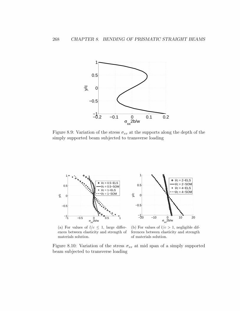
268 CHAPTER 8. BENDING OF PRISMATIC STRAIGHT BEAMS
−0.2 −0.1 0 0.1 0.2−1
−0.5
0
0.5
1
y/c
σxx
2b/w
Figure 8.9: Variation of the stress σxx at the supports along the depth of thesimply supported beam subjected to transverse loading
−1 −0.5 0 0.5 1−1
−0.5
0
0.5
1
σxx
2b/w
y/c
l/c = 0.5−ELSl/c = 0.5−SOMl/c = 1−ELSl/c = 1−SOM
(a) For values of l/c ≤ 1, large differ-ences between elasticity and strength ofmaterials solution.
−20 −10 0 10 20−1
−0.5
0
0.5
1
σxx
2b/w
y/c
l/c = 2−ELSl/c = 2−SOMl/c = 4−ELSl/c = 4−SOM
(b) For values of l/c > 1, negligible dif-ferences between elasticity and strengthof materials solution.
Figure 8.10: Variation of the stress σxx at mid span of a simply supportedbeam subjected to transverse loading

8.2. SYMMETRICAL BENDING 269
−1 −0.5 0−1
−0.5
0
0.5
1
y/c
σyy
2b/w
Figure 8.11: Variation of the stress σyy along the depth of the simply sup-ported beam subjected to transverse loading
Comparing equations (8.144) and (8.145) it can be seen that when l/c 1the results are approximately the same. Thus, again we find that for longbeams with l/c > 10 the strength of materials solution is close to the elasticitysolution. Note that from equation 8.125, the x component of displacementindicates that plane sections do not remain plane. However, for well propor-tioned beams, i.e. beams with l/c > 10, the deviation from being plane isinsignificant.
Simply supported beam subjected to sinusoidal loading
Finally, we consider a simply supported rectangular cross section beam sub-jected to sinusoidally varying transverse load along its top edge as shown inFig 8.12. Now, we shift the coordinate origin to the left end surface of thebeam. Consequently, the beam in its initial state is assumed to occupy a re-gion in the Euclidean point space defined by B = (x, y, z)|0 ≤ x ≤ 2l,−c ≤y ≤ c,−b ≤ z ≤ b.
The traction boundary conditions for this problem are
t(ey)(x, c) = − qo2b
sin(πx
l
)ey, (8.146)
t(−ey)(x,−c) = o, (8.147)

270 CHAPTER 8. BENDING OF PRISMATIC STRAIGHT BEAMS
y
x
qol/π
2c
2l
qol/π
qosin(πx/l)
Figure 8.12: Simply supported beam subjected to sinusoidally varying trans-verse load
∫ c
−c2bt(ex)(l, y)dy =
qoπley, (8.148)∫ c
−c2bt(−ex)(0, y)dy =
qoπley, (8.149)
∫ c
−c2b(yey + zez) ∧ t(ex)(l, y)dy = o, (8.150)∫ c
−c2b(yey + zez) ∧ t(−ex)(0, y)dy = o. (8.151)
The conditions (8.146) through (8.151) on assuming that the beam is sub-jected to a plane state of stress, translates into requiring
σxy(x,±c) = 0, (8.152)
σyy(x, c) = − q0
2bsin(πx/l), (8.153)
σyy(x,−c) = 0, (8.154)
∫ c
−c2bσxy(0, y)dy = −q0l/π, (8.155)∫ c
−c2bσxy(l, y)dy = q0l/π, (8.156)

8.2. SYMMETRICAL BENDING 271∫ c
−c2bσxx(0, y)dy = 0, (8.157)∫ c
−c2bσxx(l, y)dy = 0, (8.158)
∫ c
−c2bσxx(0, y)ydy = 0, (8.159)∫ c
−c2bσxx(l, y)ydy = 0, (8.160)
(8.161)
As before, we solve this boundary value problem using stress approach.Towards this, we assume the following form for the Airy’s stress function
φ = sin(βx) [A1 + A3βy] sinh(βy) + [A2 + A4βy] cosh(βy) , (8.162)
where Ai’s are constants to be determined from boundary conditions. Itis straightforward to verify that the above choice of Airy’s stress function,(8.162) satisfies the bi-harmonic equation.
Then, the Cartesian components of the stress for the assumed Airy’sstress function (8.162) is
σxx = β2 sin(βx)A1 sinh(βy)+A3 [yβ sinh(βy) + 2 cosh(βy)]+A2 cosh(βy)
+ A4 [βy cosh(βy) + 2 sinh(βy)], (8.163)
σyy = −β2 sin(βx) [A1 + A3βy] sinh(βy) + [A2 + A4βy] cosh(βy) ,(8.164)
σxy = β2 cos(βx)A1 cosh(βy) + A3 [βy cosh(βy) + sinh(βy)] + A2 sinh(βy)
+ A4 [βy sinh(βy) + cosh(βy)]. (8.165)
Now applying the boundary condition we evaluate the constants, Ai’s.The condition 8.152 implies that
A1 cosh(βc) + A3 [βc cosh(βc) + sinh(βc)] + A2 sinh(βc)
+ A4 [βc sinh(βc) + cosh(βc)] = 0. (8.166)
272 CHAPTER 8. BENDING OF PRISMATIC STRAIGHT BEAMS
A1 cosh(βc)− A3 [βc cosh(βc) + sinh(βc)]− A2 sinh(βc)
+ A4 [βc sinh(βc) + cosh(βc)] = 0. (8.167)
Adding equations (8.166) and (8.167) we obtain,
A1 cosh(βc) + A4 [βc sinh(βc) + cosh(βc)] = 0, (8.168)
Subtracting equations (8.166) and (8.167) we obtain,
A2 sinh(βc) + A3 [βc cosh(βc) + sinh(βc)] = 0. (8.169)
We write A1 in terms of A4 using equation (8.168) as
A1 = −A4[βc tanh(βc) + 1]. (8.170)
Similarly, we write A2 in terms of A3 using equation (8.169) as
A2 = −A3[βc coth(βc) + 1]. (8.171)
Substituting equations (8.170) and (8.171) in (8.164)
σyy = −β2 sin(βx)A4 [βy cosh(βy)− (βc tanh(βc) + 1) sinh(βy)]
+ A3 [βy sinh(βy)− (βc coth(βc) + 1) cosh(βy)]. (8.172)
Applying boundary condition (8.154) we obtain a relation between A3 andA4 as
A3 = −A4 tanh(βc)βc− sinh(βc) cosh(βc)
βc+ sinh(βc) cosh(βc). (8.173)
The boundary condition (8.153) requires
q0 sin(πx
l) = 2β2 sin(βx)
[βc− sinh(βc) cosh(βc)
cosh(βc)
]A4. (8.174)
In order for equation 8.174 to be true for all x, β = π/l, and so A4 isdetermined as,
A4 =q0 cosh
(πcl
)4bπ
2
l2
[πcl− sinh
(πcl
)cosh
(πcl
)] . (8.175)
It can be verified that for these choice of constants, boundary conditions(8.155) through (8.160) is satisfied. Thus, we have found a stress function

8.2. SYMMETRICAL BENDING 273
that satisfies the bi-harmonic equation and the traction boundary conditionsand therefore is a solution to the boundary value problem.
The displacements are determined through integration of the strain dis-placement relations. Since the steps in its computation is same as in theabove two examples, only the final results are recorded here
ux = − βE
cos(βx)A1[1 + ν] sinh(βy) + A2[1 + ν] cosh(βy)
+ A3 [(1 + ν)βy sinh(βy) + 2 cosh(βy)]
+ A4 [(1 + ν)βy cosh(βy) + 2 sinh(βy)] − C0y + C1, (8.176)
uy = − βE
sin(βx)A1[1 + ν] cosh(βy) + A2[1 + ν] sinh(βy)
+ A3 [(1 + ν)βy cosh(βy)− (1− ν) sinh(βy)]
+ A4 [(1 + ν)βy sinh(βy)− (1− ν) cosh(βy)]+ C0x+ C2, (8.177)
where Ci’s are constants to be determined from displacement boundary con-ditions. As before, to model a simply supported beam, we choose displace-ment boundary conditions as
ux(0, 0) = uy(0, 0) = uy(l, 0) = 0. (8.178)
The constant Ci’s determined using the above displacement conditions is
C0 = C2 = 0, C1 =β
E[A2 (1 + ν) + 2A3] . (8.179)
In order to facilitate comparison of this displacement field with that ob-tained from strength of materials approach, the vertical displacement of thecenterline is determined from equation (8.177) as
uy(x, 0) =A4β
Esin(βx) [2 + (1 + ν)βc tanh(βc)] . (8.180)
For the case when l c, we approximately computeA4 asA4 ≈−3q0l5/8bc3π5,
and so the equation (8.180) becomes
uy(x, 0) = − 3q0l4
4bc3π4Esin(πxl
)[1 +
1 + ν
2
πc
ltanh
(πcl
)]. (8.181)

274 CHAPTER 8. BENDING OF PRISMATIC STRAIGHT BEAMS
P y
z
θ
(a) Actual loading.
P*sin(θ)
y
z
P*cos(θ)
(b) Load resolved along the axis of sym-metry.
Figure 8.13: Schematic of transverse loading of a beam with rectangular crosssection
Without going into the details, the vertical deflection of the beam com-puted using strength of materials approach is,
∆ = − 3q0l4
4bc3π4Esin(πxl
). (8.182)
When l/c > 10 it can be seen that both the elasticity and strength of materialssolution is in agreement as expected.
8.3 Asymmetrical bending
Having shown that for the symmetrical bending the strength of materialapproximation is robust when l/c > 10, we proceed to use the same approx-imation for asymmetrical bending. In the case of asymmetrical bending theloading plane does not coincide with the plane of symmetry. As an illustra-tion, consider the rectangular section, loaded as shown in the figure 8.13a.The applied load can be resolved along the symmetry plane, as shown in fig-ure 8.13b. Thus, the beam bends in both the xy plane due to loading alongy direction and the xz plane due to loading along the z direction. As per thestrength of materials assumption that the plane section before deformation

8.3. ASYMMETRICAL BENDING 275
remain plane and that the sections normal to the neutral axis, remain normalafter the deformation, the displacement field for this case is,
u = −
[y − yo]d∆y
dx+ [z − zo]
d∆z
dx
ex + ∆y(x)ey + ∆z(x)ez, (8.183)
where ∆y(x) and ∆z(x) are yet to be determined functions of x, yo and zoare constants. The above displacement field is obtained by superposing thebending displacement due to transverse loading along one symmetric plane,say xy plane, (8.29) and the displacement filed due to loading along anothersymmetric plane say xz (obtained by substituting z in place of y in equation(8.29)). Recollect from section 7.5.2 that for the linear elastic material thatwe are studying, we can superpose solutions as long as the displacements aresmall.
As required in the displacement approach, we next compute the linearizedstrain corresponding to the displacement field, (8.183) as
ε =
−
[y − yo]d2∆y
dx2+ [z − zo]d
2∆z
dx2
0 0
0 0 00 0 0
. (8.184)
Then, using the 1 dimensional constitutive relation, the stress is obtained as
σxx = −E
[y − yo]d2∆y
dx2+ [z − zo]
d2∆z
dx2
. (8.185)
Substituting (8.185) in equation (8.3) and using the condition that no axialload is applied we obtain∫∫
a
E
[y − yo]
d2∆y
dx2+ [z − zo]
d2∆z
dx2
dydz = 0. (8.186)
For equation (8.186) to hold we require that∫∫a
E[y − yo]dydz = 0,
∫∫a
E[z − zo]dydz = 0, (8.187)
since in equation (8.186) ∆y and ∆z are independent functions of x and inparticular ∆y 6= −k∆z, where k is a constant. From equation (8.187) weobtain,
yo =
∫∫aEydydz∫∫aEdydz
, zo =
∫∫aEzdydz∫∫aEdydz
. (8.188)

276 CHAPTER 8. BENDING OF PRISMATIC STRAIGHT BEAMS
If the beam is also homogeneous then Young’s modulus, E is a constant andtherefore,
yo = (
∫∫a
ydydz)/(
∫∫a
dydz), zo = (
∫∫a
zdydz)/(
∫∫a
dydz), (8.189)
the y and z coordinates of the centroid of the cross section. Without loss ofgenerality the origin of the coordinate system can be assumed to be locatedat the centroid of the cross section and hence yo = zo = 0.
Since, we have assumed that there is no net applied axial load, i.e.,∫a
σxxda = 0, (8.190)
equation (8.9) and (8.8) can be written as,
Mz = −∫a
yσxxda = −∫a
yσxxda+
∫a
yoσxxda = −∫a
[y − yo]σxxda,
(8.191)
My =
∫a
zσxxda =
∫a
zσxxda−∫a
zoσxxda =
∫a
[z − zo]σxxda, (8.192)
where yo and zo are constants as given in equation (8.188). Substitutingequation (8.185) in equation (8.191) we obtain,
Mz =
∫∫a
[y − yo]2Ed2∆y
dx2dydz +
∫∫a
[y − yo][z − zo]Ed2∆z
dx2dydz
=d2∆y
dx2
∫∫a
[y − yo]2Edydz +d2∆z
dx2
∫∫a
[y − yo][z − zo]Edydz. (8.193)
If the cross section of the beam is homogeneous, the above equation can bewritten as,
Mz =d2∆y
dx2E
∫∫a
[y − yo]2dydz +d2∆z
dx2E
∫∫a
[y − yo][z − zo]dydz
=d2∆y
dx2EIzz +
d2∆z
dx2EIyz, (8.194)

8.3. ASYMMETRICAL BENDING 277
where,
Izz =
∫∫a
[y − yo]2dydz, Iyz =
∫∫a
[y − yo][z − zo]dydz, (8.195)
are the moment of inertia about the z axis, the axis about which the ap-plied forces produces a moment, Mz and the product moment of inertia.Substituting equation (8.185) in equation (8.192) we obtain,
My = −∫∫a
[y − yo][z − zo]Ed2∆y
dx2dydz −
∫∫a
[z − zo]2Ed2∆z
dx2dydz
= −d2∆y
dx2
∫∫a
[y − yo][z − zo]Edydz −d2∆z
dx2
∫∫a
[z − zo]2Edydz. (8.196)
If the cross section of the beam is homogeneous, the above equation can bewritten as,
My = −d2∆y
dx2E
∫∫a
[y − yo][z − zo]dydz −d2∆z
dx2E
∫∫a
[z − zo]2dydz
= −d2∆y
dx2EIyz −
d2∆z
dx2EIyy, (8.197)
where,
Iyy =
∫∫a
[z − zo]2dydz, (8.198)
is the moment of inertia about the y axis, the axis about which the appliedforces produces a moment, My. Solving equations (8.194) and (8.197) for ∆y
and ∆z we obtain,
d2∆y
dx2=IyzMy + IyyMz
E[IyyIzz − I2yz],
d2∆z
dx2= −IyzMz + IzzMy
E[IyyIzz − I2yz]. (8.199)
Substituting (8.199) in (8.185) we obtain
σxx = −[y − yo]IyzMy + IyyMz
IyyIzz − I2yz
+ [z − zo]IyzMz + IzzMy
IyyIzz − I2yz
, (8.200)

278 CHAPTER 8. BENDING OF PRISMATIC STRAIGHT BEAMS
P y
z
θ
Neutral surface
β
Figure 8.14: Schematic showing the neutral surface for a beam with rectan-gular cross section subjected to transverse loading
where yo and zo are as given in equation (8.189). Equation (8.200) givesthe bending normal stress when a cross section is subjected to both My andMz bending moments or when the cross section is subjected to a bendingmoment about an axis for which the product moment of inertia is not 0, i.e.,loading is not along a plane of symmetry.
Before proceeding further, a few observations on equation (8.200) have tobe made. It is clear from the equation (8.200) that the bending normal stressvaries linearly over the cross sectional surface. As in the case of symmetricalbending, there exist a surface which has zero bending normal stress. Thiszero bending normal stress surface, called as the neutral surface is defined by
tan(β) =y − yoz − zo
=IyzMz + IzzMy
IyzMy + IyyMz
. (8.201)
Figure 8.14 shows a typical neutral surface for a beam with rectangular crosssection subjected to transverse loading not in the plane of symmetry of thecross section.
Having found the bending normal stress, next we find the bending shearstress. Towards this, we consider the equilibrium of a cuboid pqrstuvw asshown in figure 8.15, taken from a beam subjected to asymmetric bendingmoment that varies along the longitudinal axis of the beam. Note that onthis cuboid, bending normal stress σ−xx acts on the face prtv and σ+
xx acts onthe face qsuw, shear stress, σxy acts in plane rsvw and shear stress, σxz acts

8.3. ASYMMETRICAL BENDING 279
x
y
z
p
r s q
u t v w
Figure 8.15: Schematic of a section of a beam with rectangular cross sectionto find the shear stresses due to asymmetric loading
in plane tuvw. Now, the force balance along the x direction requires that
σxy(∆x)(b− z) + σxz(∆x)(c− y) +
∫∫a
[σ+xx − σ−xx]dzdy = 0, (8.202)
where we have assumed that constant shear stresses act on faces rsvw andpqrs and that the bending normal stress varies linearly over the faces prtvand qsuw as indicated in equation (8.200). Appealing to Taylor’s series, wewrite,
σ+xx = σ−xx +
dσxxdx
(∆x), (8.203)
truncating the series after first order term, since our interest is in the limit(∆x) tending to zero. Differentiating (8.200) with respect to x we obtain,
dσxxdx
= − [y − yo][IzzIyy − I2
yz]
[Iyy
dMz
dx+ Iyz
dMy
dx
]+
[z − zo][IzzIyy − I2
yz]
[Iyz
dMz
dx+ Izz
dMy
dx
](8.204)
Substituting equations (8.18) and (8.20) in (8.204),
dσxxdx
= − [y − yo][IzzIyy − I2
yz][−IyyVy + IyzVz] +
[z − zo][IzzIyy − I2
yz][−IyzVy + IzzVz] .
(8.205)
280 CHAPTER 8. BENDING OF PRISMATIC STRAIGHT BEAMS
Substituting equation (8.205) in (8.203) and using the resulting equation in(8.202) we obtain
σxy(b− z) + σxz(c− y) = − [IyyVy − IyzVz][IzzIyy − I2
yz]
c∫y
[y − yo]b∫
z
dz
dy
− [IzzVz − IyzVy][IzzIyy − I2
yz]
b∫z
[z − zo]c∫
y
dy
dz, (8.206)
where the limits of the integration have been arrived at for the rectangu-lar cross section shown in figure 8.15. Thus, if the section is thick walled,equation (8.206) is insufficient to determine all the shear stresses as such.Hence, strength of materials approach cannot yield the shear stresses in athick walled section subjected to asymmetrical loading. However, it shouldbe mentioned that the shear stresses in a well proportioned thick walled sec-tion, with l/c > 10, for which the strength of materials solution is applicable,will develop shear stresses which are an order of magnitude, at least, less thanthat of the bending stresses.
On the other hand since the direction of the shear stress is well definedin thin walled sections. It is going to be tangential to the cross section atthe point of interest, as in the case of symmetric bending. Further, by virtueof the section being thin walled, we assume the shear stresses to be uniformacross its thickness, t. Now, the shear stress, τ acting as shown in figure 8.16balances the imbalance created due to the variation of the bending normalstresses along the longitudinal axis of the beam. Following the same stepsas in the case of thick walled cross sections detailed above, it can be shownthat
τ = −1
t
[IyyVy − IyzVz][IzzIyy − I2
yz]
∫a
[y − yo]dydz +[IzzVz − IyzVy][IzzIyy − I2
yz]
∫a
[z − zo]dydz,
(8.207)where the area over which the integration is to be performed is the shadedregion shown in figure 8.16. If one is to use polar coordinates to describe thecross section and defining ro =
√y2o + z2
o and β = tan−1(yo/zo), the equation

8.3. ASYMMETRICAL BENDING 281
co s r
τ N.A.
p q
Δx
c t
Figure 8.16: Stresses acting on a thin walled cross section beam subjected toasymmetric loading
(8.207) can be written as,
τ = − [IyyVy − IyzVz][IzzIyy − I2
yz]
∫ α
φ
r2[sin(θ)− ro
rsin(β)
]dθ
− [IzzVz − IyzVy][IzzIyy − I2
yz]
∫ α
φ
r2[cos(θ)− ro
rcos(β)
]dθ, (8.208)
where r could be a function of θ but ro and β are constants. Thus, in equation(8.208) the shear stress, τ is a function of φ only.
While this representation is convenient in cases where the section isnot made up of straight line segments, a representation using the perime-ter length, s, of the cross section is useful when the section is made up ofstraight line segments. Thus, the expression for the shear stress in terms ofthe perimeter length as shown in figure 8.16 is,
τ = − [IyyVy − IyzVz][IzzIyy − I2
yz]
∫ s
0
[r sin(θ)−yo]ds−[IzzVz − IyzVy][IzzIyy − I2
yz]
∫ s
0
[r cos(θ)−zo]ds,
(8.209)where now r and θ have to be expressed as a function of s. Here we haveused the relation, ds = rdθ to obtain (8.209) from (8.208).
Thus, integrating the ordinary differential equations (8.199) we obtain thedeflections of the beam along the y and z directions and hence the displace-ment field for the beam, (8.183) can be computed. Using equation (8.200)the bending normal stress is evaluated. While these calculations are the samefor thin or thick walled sections, the shear stress estimation is different. Wecould not find the shear stresses in case of thick walled sections using the

282 CHAPTER 8. BENDING OF PRISMATIC STRAIGHT BEAMS
strength of materials approach. However, equation (8.207) gives the shearstresses in thin walled sections. This completes the solution to asymmetricalbending problem.
8.4 Shear center
Having found the solution to symmetrical and asymmetrical bending, in thissection we find where the load has to be applied so that it produces notorsion.
Shear center is defined as the point about which the external load has tobe applied so that it produces no twisting moment.
Recall from equation (8.7) the torsional moment due to the shear forceσxy and σxz about the origin is,
Mx =
∫a
[σxzy − σxyz]dydz. (8.210)
Since,∫aσxzdydz = Vz and
∫aσxydydz = Vy, the moment about some other
point (ysc, zsc) would be,
M scx =
∫a
[σxzy − σxyz]dydz − Vzysc + Vyzsc. (8.211)
If this point (ysc, zsc) is the shear center, then M scx = 0. Thus, we have to
find ysc and zsc such that,∫a
[σxzy − σxyz]dydz − Vzysc + Vyzsc = 0, (8.212)
holds. We have two unknowns but only one equation. Hence, we cannot findysc and zsc uniquely, in general. If the loading is such that only shear forceVy is present, then
zsc =1
Vy
∫a
[σxyz − σxzy]dydz. (8.213)
Similarly, if Vy = 0,
ysc =1
Vz
∫a
[σxzy − σxyz]dydz. (8.214)
8.4. SHEAR CENTER 283
Equations (8.213) and (8.214) are used to find the coordinates of the shearcenter with respect to the chosen origin of the coordinate system, which forhomogeneous sections is usually taken as the centroid of the cross section.Thus, the point that (ysc, zsc) are the coordinates of the shear center fromthe origin of the chosen coordinate system which in many cases would be thecentroid of the section cannot be overemphasized. In the case of thin walledsections which develop shear stresses tangential to the cross section, σxy =−τ sin(θ) and σxz = τ cos(θ), where τ is the magnitude of the shear stressand θ is the angle the tangent to the cross section makes with the z direction.
By virtue of the shear stress depending linearly on the shear force (seeequations (8.43) and (8.207)), it can be seen that the coordinates of the shearcenter is a geometric property of the section.
8.4.1 Illustrative examples
Next, to illustrate the use of equations (8.213) and (8.214) we find the shearcenter for some shapes.
Example 1: Rectangular section
The first section that we consider is a thick walled rectangular section asshown in figure 8.17 having a depth 2c and width 2b. The chosen coordinatebasis coincides with the two axis of symmetry that this section has and theorigin is at the centroid of the cross section.
First, we shall compute the z coordinate of the shear center zsc. For thisonly shear force Vy should act on the cross section. Shear force Vy would becaused due to loading along the xy plane, a plane of symmetry for the crosssection. Therefore the shear stress, σxy is computed using (8.43) as
σxy = − Vy2b(2b(2c)3/12)
(2b)
∫ c
y
ydy =3Vy8bc
[1− y2
c2
], (8.215)
where we have used the fact that yo = 0, since the origin is located at thecentroid of the cross section. Further, for this loading σxz = 0. Substituting(8.215) and σxz = 0 in (8.213) we obtain
zsc =3
8bc
∫ b
−bzdz
∫ c
−c
[1− y2
c2
]dy = 0. (8.216)

284 CHAPTER 8. BENDING OF PRISMATIC STRAIGHT BEAMS
τ
y
z 2c
2b (a) Rectangular cross section sub-jected to a shear force Vy.
τ
y
z 2c
2b (b) Rectangular cross section sub-jected to a shear force Vz.
Figure 8.17: Schematic of a rectangular cross section subjected to a shearforce along one direction
Next, we shall compute the y coordinate of the shear center ysc. Now, onlyshear force Vz should act. This shear force would be produced by loadingalong the xz plane, also a plane of symmetry for the cross section. Thisloading produces a shear stress as shown in figure 8.17b whose magnitude isagain computed using (8.43) as
σxz = − Vz2c(2c(2b)3/12)
(2c)
∫ b
z
zdz =3Vz8bc
[1− z2
b2
]. (8.217)
and σxy = 0. Substituting (8.217) in (8.214) we obtain
ysc =3
8bc
∫ c
−cydy
∫ b
−b
[1− z2
c2
]dz = 0. (8.218)
Thus, for the rectangular cross section, the shear center is located at theorigin of the coordinate system, which in turn is the centroid of the crosssection. Hence, the shear center coincides with the centroid of the crosssection.

8.4. SHEAR CENTER 285
y
z
τ
τ
τ
C
A B
D
h
b
t
(a) Channel cross section subjectedto a shear force Vy.
y
z
τ
τ
τ
C
A B
D
h
b
t
(b) Channel cross section subjectedto a shear force Vz.
Figure 8.18: Schematic of a channel cross section subjected to a shear forcealong one direction
286 CHAPTER 8. BENDING OF PRISMATIC STRAIGHT BEAMS
Example 2: Channel section
The next section that we study is the channel section with orientation anddimensions as shown in figure 8.18. The flange and web thickness of thechannel is the same. Before proceeding to compute the shear center theother geometric properties, the centroid and the moment of inertia’s for thecross section is computed. The origin of the coordinate system being used isat the centroid of the cross section. Then, the distance from the centroid ofthe cross section to the top most fiber of the cross section AB is yAB = c =h/2 + t. Similarly, the distance of the left most fiber in the web of the crosssection, BC is zBC = (ht+ 2b2)/(2(h+ 2b)). Now,
Iyz = 0, (8.219)
Izz =1
12
[th3 + 2bt3
]+
1
2bt(h+ t)2, (8.220)
Iyy =1
12
[ht3 + 2tb3
]+ ht
(zBC −
t
2
)2
+ 2bt
(b
2− zBC
)2
=1
12
[ht3 + 2tb3
]+ht
4
(b(b− 2t)
(h+ 2b)
)2
+bt
2
(h(b− t)(h+ 2b)
)2
. (8.221)
Towards computing the location of the shear center along the z direction,we first compute the shear stress acting on the cross section due to a shearforce Vy alone. The magnitude of the shear stress, τ is found using (8.209)as
τ =
− VyIzz
(h+t)2
∫ s0ds 0 ≤ s ≤
(b− t
2
)− VyIzz
[(h+t)
2
∫ b−t/20
ds
+∫ sb−t/2
[(h+t)
2−(s− b+ t
2
)]ds] (
b− t2
)≤ s ≤
(b+ h+ t
2
)− VyIzz
[(h+t)
2
∫ b−t/20
ds− (h+t)2
∫ sb+h+t/2
ds
+∫ b+h+t/2
b−t/2
[(h+t)
2−(s− b+ t
2
)]ds] (
b+ h+ t2
)≤ s ≤ (2b+ h)
.
(8.222)
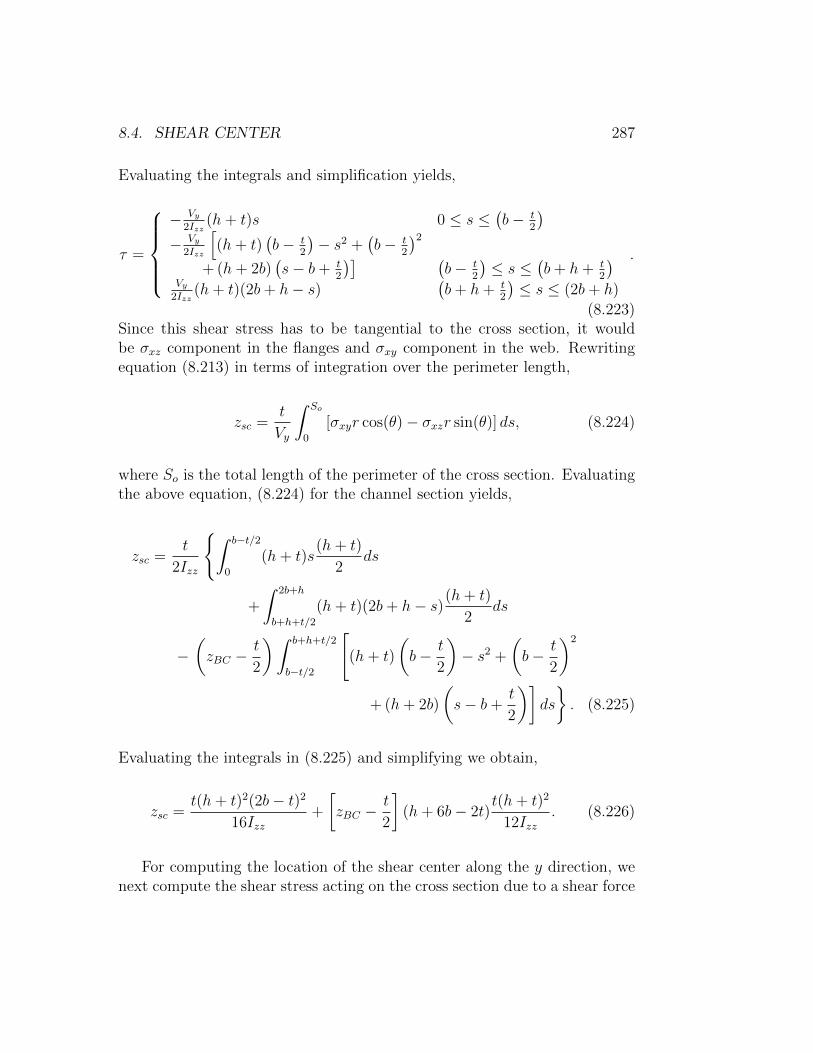
8.4. SHEAR CENTER 287
Evaluating the integrals and simplification yields,
τ =
− Vy
2Izz(h+ t)s 0 ≤ s ≤
(b− t
2
)− Vy
2Izz
[(h+ t)
(b− t
2
)− s2 +
(b− t
2
)2
+ (h+ 2b)(s− b+ t
2
)] (b− t
2
)≤ s ≤
(b+ h+ t
2
)Vy
2Izz(h+ t)(2b+ h− s)
(b+ h+ t
2
)≤ s ≤ (2b+ h)
.
(8.223)Since this shear stress has to be tangential to the cross section, it wouldbe σxz component in the flanges and σxy component in the web. Rewritingequation (8.213) in terms of integration over the perimeter length,
zsc =t
Vy
∫ So
0
[σxyr cos(θ)− σxzr sin(θ)] ds, (8.224)
where So is the total length of the perimeter of the cross section. Evaluatingthe above equation, (8.224) for the channel section yields,
zsc =t
2Izz
∫ b−t/2
0
(h+ t)s(h+ t)
2ds
+
∫ 2b+h
b+h+t/2
(h+ t)(2b+ h− s)(h+ t)
2ds
−(zBC −
t
2
)∫ b+h+t/2
b−t/2
[(h+ t)
(b− t
2
)− s2 +
(b− t
2
)2
+ (h+ 2b)
(s− b+
t
2
)]ds
. (8.225)
Evaluating the integrals in (8.225) and simplifying we obtain,
zsc =t(h+ t)2(2b− t)2
16Izz+
[zBC −
t
2
](h+ 6b− 2t)
t(h+ t)2
12Izz. (8.226)
For computing the location of the shear center along the y direction, wenext compute the shear stress acting on the cross section due to a shear force

288 CHAPTER 8. BENDING OF PRISMATIC STRAIGHT BEAMS
Vz alone. The magnitude of the shear stress, τ is found using (8.209) as
τ =
− VzIyy
∫ s0
(s+ zBC − b)ds 0 ≤ s ≤(b− t
2
)− VzIyy
[∫ b−t/20
(s+ zBC − b)ds
+(zBC − t
2
) ∫ sb−t/2 ds
] (b− t
2
)≤ s ≤
(b+ h+ t
2
)− VzIyy
[∫ b−t/20
(s+ zBC − b)ds+(zBC − t
2
) ∫ b+h+t/2
b−t/2 ds
+∫ sb+h+t/2
(h− s+ zBC + b)ds] (
b+ h+ t2
)≤ s ≤ (2b+ h)
.
(8.227)Integrating the above equation we obtain,
τ =
− VzIyy
[s2
2+ (zBC − b)s
]0 ≤ s ≤
(b− t
2
)− VzIyy
[(2b−t)2
8+ (zBC − b) (2b−t)
2
+(zBC − t
2
) (s− (2b−t)
2
)] (b− t
2
)≤ s ≤
(b+ h+ t
2
)− VzIyy
[(2b−t)2
8+ (zBC − b) (2b−t)
2
+(zBC − t
2
)(h+ t)− s2
2
+ (b+h+t/2)2
2
+(zBC + b+ h)(s− b− h− t
2
)] (b+ h+ t
2
)≤ s ≤ (2b+ h)
.
(8.228)Since this shear stress has to be tangential to the cross section, as before,it would be σxz component in the flanges and σxy component in the web.Rewriting equation (8.214) in terms of integration over the perimeter length,
ysc = − t
Vz
∫ So
0
[σxyr cos(θ)− σxzr sin(θ)] ds, (8.229)
where So is the total length of the perimeter of the cross section. Evaluating

8.4. SHEAR CENTER 289
the above equation, (8.229) for the channel section yields,
ysc = − t
Iyy
(h+ t)
2
∫ b−t/2
0
[s2
2+ (zBC − b)s
]ds
−(zBC −
t
2
)∫ b+h+t/2
b−t/2
[(2b− t)2
8+ (zBC − b)
(2b− t)2
+
(zBC −
t
2
)(s− (2b− t)
2
)]ds
− (h+ t)
2
∫ 2b+h
b+h+t/2
[(2b− t)2
8+ (zBC − b)
(2b− t)2
+
(zBC −
t
2
)(h+ t)− s2
2
+(b+ h+ t/2)2
2+ (zBC + b+ h)
(s− b− h− t
2
)]ds
(8.230)
Evaluating the integrals and simplifying, we find that ysc = 0!
Example 3: Circular arc
The final section that we use to illustrate the procedure to find the shearcenter is an arc of a circular section with radius R and a uniform thicknesst. The arc is assumed to span from −(π − α) ≤ θ ≤ (π − α). Thus, it issymmetrical about the z direction. For convenience, we assume the originof the coordinate system to be located at the center of the circle. First, wecompute the centroid of the cross section,
yo =
∫ayda∫ada
=
∫ π−α−(π−α)
R sin(θ)t(Rdθ)∫ π−α−(π−α)
t(Rdθ)= 0, (8.231)
zo =
∫azda∫ada
=
∫ π−α−(π−α)
R cos(θ)t(Rdθ)∫ π−α−(π−α)
t(Rdθ)= R
sin(α)
(π − α). (8.232)
Here we have identified yo and zo with the coordinates of the centroid of thecross section, since it is homogeneous. Next, we compute the moment ofinertias about the centroid,
Izz =
∫a
[y − yo]2da =
∫ π−α
−(π−α)
[R sin(θ)− 0]2t(Rdθ)
= R3t
[π − α +
1
2sin(2α)
], (8.233)
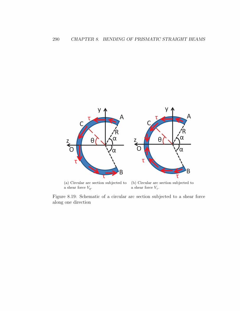
290 CHAPTER 8. BENDING OF PRISMATIC STRAIGHT BEAMS
y
z α
α θ
A C
O
B
R
τ
τ
τ
(a) Circular arc section subjected toa shear force Vy.
y
z α
α θ
A C
O
B
R
τ
τ
τ
(b) Circular arc section subjected toa shear force Vz.
Figure 8.19: Schematic of a circular arc section subjected to a shear forcealong one direction

8.4. SHEAR CENTER 291
Iyz =
∫a
[y − yo][z − zo]da =
∫ π−α
−(π−α)
[R sin(θ)− 0][R cos(θ)− zo]t(Rdθ) = 0.
(8.234)
Iyy =
∫a
[z − zo]2da =
∫ π−α
−(π−α)
[R cos(θ)− zo]2t(Rdθ)
= R3t
[(1 + 2
z2o
R2
)(π − α)− 1
2sin(2α)− 4
zoR
sin(α)
]= R3t
[π − α− 2
sin2(α)
π − α− 1
2sin(2α)
], (8.235)
where the last equality is obtained on substituting for zo from (8.232).
Towards computing the z coordinate of the shear center, we compute theshear stress distribution in the circular arc when only shear force Vy is actingon the cross section. The magnitude of the shear stress, τ is found using(8.208) as,
τ = − VyIzz
∫ π−α
φ
R2 sin(θ)dθ = − VyIzz
R2[cos(α) + cos(φ)]. (8.236)
This shear stress would act tangential to the cross section at every locationas indicated in figure 8.19a. Therefore, σxy = −τ cos(φ) and σxz = τ sin(φ),where φ is the angle the tangent makes with the y axis. Appealing to equation(8.213) we obtain,
zsc = − 1
Vy
∫ π−α
−(π−α)
[τ cos(φ)(R cos(φ)) + τ sin(φ)(R sin(φ))] tRdφ
=R4t
Izz
∫ π−α
−(π−α)
[cos(α) + cos(φ)]dφ = R4[(π − α) cos(α) + sin(α)]
[2(π − α) + sin(2α)], (8.237)
where we have used equations (8.236) and (8.233) respectively. It can beseen that when 0 < α ≤ π/2, zsc > 0 and in fact R < zsc ≤ 4R/π.
Next, for computing the y coordinate of the shear center, we computethe shear stress distribution in the circular arc when only shear force Vz isacting on the cross section. The magnitude of the shear stress, τ is found

292 CHAPTER 8. BENDING OF PRISMATIC STRAIGHT BEAMS
using (8.208) as,
τ = − VzIyy
∫ π−α
φ
R2
[cos(θ)− sin(α)
(π − α)
]dθ
= − VzIyy
R2
[sin(α)
φ
(π − α)− sin(φ)
]. (8.238)
This shear stress would act tangential to the cross section at every locationas indicated in figure 8.19b. Hence, as before, σxy = −τ cos(φ) and σxz =τ sin(φ), where φ is the angle the tangent makes with the y axis. Appealingto equation (8.214) we obtain,
ysc =1
Vz
∫ π−α
−(π−α)
[τ cos(φ)(R cos(φ)) + τ sin(φ)(R sin(φ))] tRdφ
= −R4t
Iyy
∫ π−α
−(π−α)
[sin(α)
φ
(π − α)− sin(φ)
]dφ = 0, (8.239)
where we have used equations (8.238) and (8.235) respectively. Thus, theshear center is located along the z axis.
By virtue of the zsc being greater than R, the shear center is locatedoutside the cross section. Hence, for the loading to pass through the shearcenter similar issues as discussed in the channel section exist.
8.5 Summary
In this chapter we solved boundary value problems corresponding to bendingof straight, prismatic members. We obtained the solution - the stress anddisplacement field - by assuming the displacement field in the strength ofmaterials approach and the stress field in the elasticity approach. We alsocompared the solutions and found good agreement between the solution ob-tained by both these approaches, when the length to depth ratio of thesemembers are greater than 10, for the case when the loading passes through aplane of symmetry. Then, we studied asymmetric bending and obtained thesolution by starting with an assumption on the displacement field. Thoughwe did not obtain the elasticity solution for this case, it can be obtained byusing principle of superposition and leave it as an exercise to the student towork the details. Then we introduced an concept called the shear center. It

8.6. SELF-EVALUATION 293
y
x
2l
2c
w
wl 2wl2
Figure 8.20: Cantilever beam subjected to uniformly distributed load on topsurface. Figure for problem 2
is the point about which the external load has to be applied so that there isno twisting of cross section. We outlined a method to find this shear centerand illustrated the same for three sections.
8.6 Self-Evaluation
1. Find the displacement and stress fields in a cantilever beam with rect-angular cross section of length 2l, depth 2c and width 2b subjected toa pure bending moment by assuming that plane section remain planeand normal to the neutral axis. Solve the same problem by assuming acubic polynomial for the Airy’s stress function. Compare the solutionsand draw inferences.
2. Find the displacement and stress fields in a cantilever beam with rect-angular cross section of length 2l, depth 2c and width 2b subjected to auniformly distributed load on the top surface, as shown in figure 8.20,by assuming that plane section remain plane and normal to the neutralaxis. Solve the same problem by assuming a suitable polynomial forthe Airy’s stress function. Compare the solutions and draw inferences.
3. A simply supported wood beam of rectangular cross section carries a

294 CHAPTER 8. BENDING OF PRISMATIC STRAIGHT BEAMS
AB
y
z
y1
z1
l
b
h
Figure 8.21: Simply supported beam subjected to uniformly distributed loadon top surface with the load not acting in the plane of symmetry. Figure forproblem 3
uniform load of intensity, w as shown in figure 8.21. The plane ofsymmetry of the beam, x1y1 plane, is inclined to the vertical xy-planeof loading by an angle α as shown. Calculate the maximum bendingstresses if l = 3 m, w = 3 kN/m, b = 0.15 m, h = 0.2 m and tan(α) =0.5.
4. For the T-section shown in figure 8.22 find the shear center. The di-mensions in the figure are in millimeters.
5. For the homogeneous trapezoidal cross section shown in figure 8.23show that the neutral surface is located at a distance, c2 = h(b2 +2b1)/(3(b2 + b1)), from the bottom of the section. Also calculate thelocation of the shear center.

8.6. SELF-EVALUATION 295
80
60
20
20
Figure 8.22: T-section. Dimensions in mm. Figure for problem 4
b2
b1
hc1
c2
NS
Figure 8.23: Trapezoidal section. NS stands for neutral surface. Figure forproblem 5

296 CHAPTER 8. BENDING OF PRISMATIC STRAIGHT BEAMS
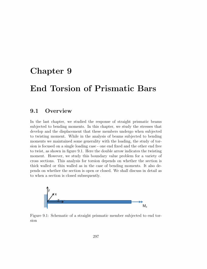
Chapter 9
End Torsion of Prismatic Bars
9.1 Overview
In the last chapter, we studied the response of straight prismatic beamssubjected to bending moments. In this chapter, we study the stresses thatdevelop and the displacement that these members undergo when subjectedto twisting moment. While in the analysis of beams subjected to bendingmoments we maintained some generality with the loading, the study of tor-sion is focused on a single loading case - one end fixed and the other end freeto twist, as shown in figure 9.1. Here the double arrow indicates the twistingmoment. However, we study this boundary value problem for a variety ofcross sections. This analysis for torsion depends on whether the section isthick walled or thin walled as in the case of bending moments. It also de-pends on whether the section is open or closed. We shall discuss in detail asto when a section is closed subsequently.
Mz z x
y
Figure 9.1: Schematic of a straight prismatic member subjected to end tor-sion
297

298 CHAPTER 9. END TORSION OF PRISMATIC BARS
Before proceeding further, we would like to point out the change in theorientation of the coordinate system, from that used in the study of thebeams. This is necessitated because for some problems we would be usingcylindrical polar coordinates, and want the cross section to be in the xyplane. We use cylindrical polar coordinates with this orientation so thatthe boundary of the cross section can be defined easily. Since, the value ofdisplacement or stress in a material particle is independent of the coordinatesystem used, it is expected that the analyst pick coordinate systems that isconvenient for a problem and not that which he is comfortable with. Hence,the change.
For this orientation of the coordinate system, following the same steps asdiscussed in detail in chapter 8, it can be shown that the torsional moment,Mz is given by,
Mz =
∫a
(σyzx− σxzy)dxdy, (9.1)
and for completeness, the other two components of the moment, which arebending moments are,
My = −∫a
σzzxdxdy, (9.2)
Mx =
∫a
σzzydxdy. (9.3)
Comparing equations (9.1) with (9.2) and (9.3) it can be seen that whilethe bending moments are due to normal stresses, torsional moment is dueto shear stresses. This is the major difference between the bending andtwisting moment. While the bending moment gives raise to normal stressespredominantly, twisting moment gives raise to shear stresses predominantly.
Now let us see how to classify the sections. As in case of bending, a crosssection would be classified as thin walled if the thickness of the cross sectionis such that it is much less than the characteristic dimensions of the crosssection. Typically, if the ratio of the thickness of the cross section to thelength of the member is less than 0.1, the section is classified as thin. If thesection is not thin, it is considered to be thick.
If a section when twisted can deform such that plane sections beforedeformation remain plane after twisting is called closed section. Sectionswhich do not deform in the above manner are called open sections. SolidCircular cross section is an example of closed section and solid rectangular
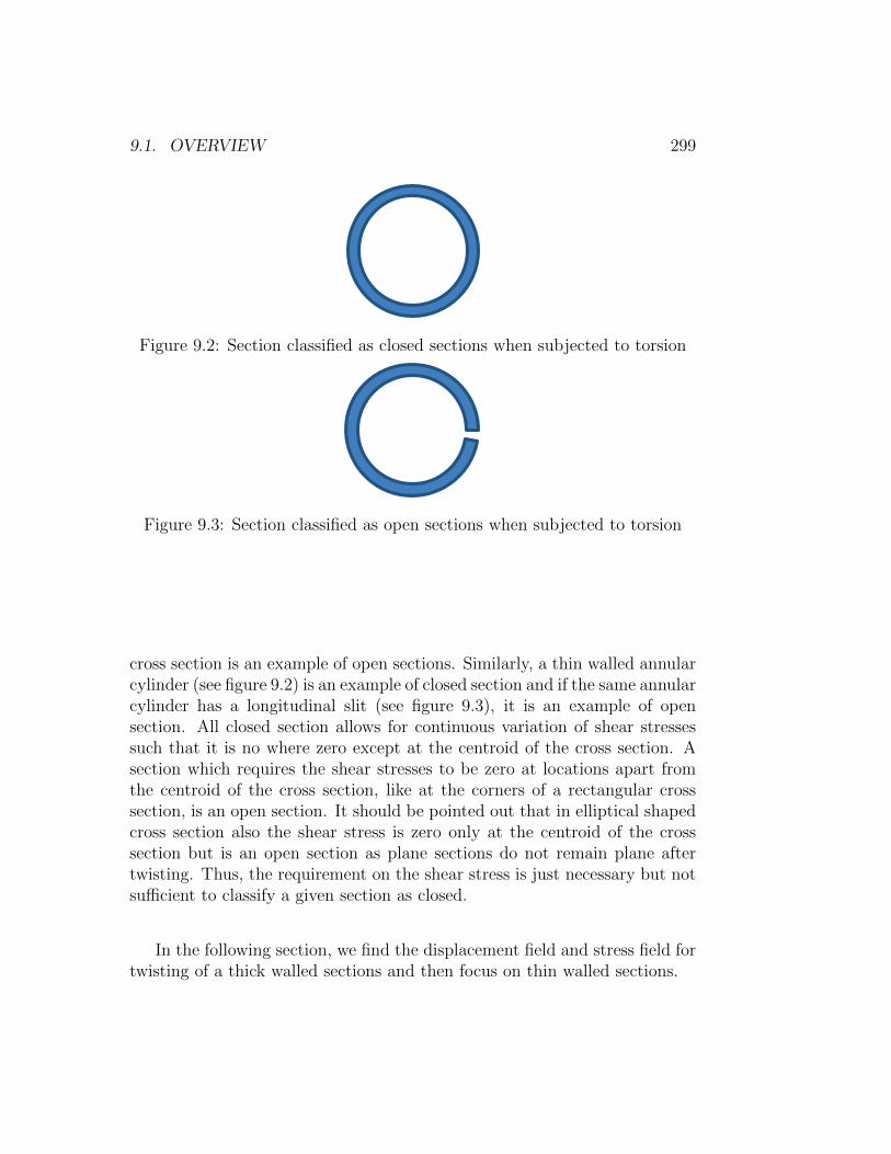
9.1. OVERVIEW 299
Figure 9.2: Section classified as closed sections when subjected to torsion
Figure 9.3: Section classified as open sections when subjected to torsion
cross section is an example of open sections. Similarly, a thin walled annularcylinder (see figure 9.2) is an example of closed section and if the same annularcylinder has a longitudinal slit (see figure 9.3), it is an example of opensection. All closed section allows for continuous variation of shear stressessuch that it is no where zero except at the centroid of the cross section. Asection which requires the shear stresses to be zero at locations apart fromthe centroid of the cross section, like at the corners of a rectangular crosssection, is an open section. It should be pointed out that in elliptical shapedcross section also the shear stress is zero only at the centroid of the crosssection but is an open section as plane sections do not remain plane aftertwisting. Thus, the requirement on the shear stress is just necessary but notsufficient to classify a given section as closed.
In the following section, we find the displacement field and stress field fortwisting of a thick walled sections and then focus on thin walled sections.

300 CHAPTER 9. END TORSION OF PRISMATIC BARS
9.2 Twisting of thick walled closed section
First, we study the twisting of thick walled closed section and then thin walledclosed section. This problem we study using the displacement approach. Wealso use cylindrical polar coordinates to formulate and study the problem.While the solution that we obtain does not require that the cross section tobe closed section be circular, we shall assume this for illustration purpose,mainly to fix the geometry of the body. Thus, we assume the body to be anright circular annular (or solid) cylinder occupying a region in the Euclideanpoint space given by: B = (r, θ, z)|Ri ≤ r ≤ Ro, 0 ≤ θ ≤ 2π, 0 ≤ z ≤ L,where Ri, Ro and L are constants with Ri = 0 in case of solid cylinder. Since,we are interested in this body being subjected to pure torsional moment, thetraction boundary conditions are
t(er)(Ro, θ, z) = o, t(er)(Ri, θ, z) = o, (9.4)∫a
t(−ez)(r, θ, 0)da = o,
∫a
t(ez)(r, θ, L)da = o, (9.5)∫a
rer ∧ t(−ez)(r, θ, 0)da = −Tez,
∫a
rer ∧ t(ez)(r, θ, L)da = Tez,(9.6)
where T is a constant. Further, since one end of this body is assumed to befixed and the other end free to displace radially and circumferentially, thedisplacement boundary conditions for this problem is,
u(r, θ, 0) = o, uz(r, θ, L) = 0, (9.7)
where uz denotes the z component of the displacement field and we haveassumed that the surface of the body defined by z = 0 is fixed and the othersurfaces are free to displace radially and circumferentially.
Since, we are going to solve the problem using the displacement approach,we have to assume the displacement field. We shall assume that plane sec-tions normal to the axis of the member, ez remain plane and perpendicularto the axis. This means that the z component of the displacement field isonly a function of z, i.e., uz = uz(z). Further, the boundary condition (9.7)requires that uz(0) = uz(L) = 0. Consistent with these requirements, weassume that the z component of the displacement, uz = 0. We could havealso assumed uz = C sin(mπz/L), where m is an integer and C is a con-stant. However, it can be shown that such an assumption to satisfy balanceof linear momentum would require that C = 0. Then, we shall assume that

9.2. TWISTING OF THICK WALLED CLOSED SECTION 301
α
A B
(a) Schematic of deformation in the yz plane
φ
2Ri 2Ro
(b) Schematic of deforma-tion in the xy plane
Figure 9.4: Schematic of the deformation of a straight prismatic membersubjected to end torsion
there is no radial component of the displacement, i.e., ur = 0. Since, straightradial lines before deformation remain as straight radial lines after deforma-tion with their length unchanged, we are justified in making the assumptionthat ur = 0. Further, we assume that the straight line along the axis of themember remains straight but rotates by an angle θ and that the radial linesrotate by an angle φ as shown in the figure, 9.4 when subjected to twistingmoment. Consequently, the circumferential component of the displacement,uθ = Ωrz, where Ω is called as the angle of twist per unit length. The slopeof the straight line along the axis of the member located at a radial distance,r∗ after deformation, α = Ωr∗. Similarly, the rotation undergone by radiallines in a plane defined by z = z∗, where z∗ is a constant, is φ = Ωz∗. Thus,the displacement field is taken as,
u = Ωrzeθ. (9.8)
It can then be verified that this displacement field satisfies the displacementboundary conditions (9.7). Then, the strain field corresponding to the dis-placement field (9.8) is
ε =
0 0 00 0 Ωr
2
0 Ωr2
0
. (9.9)
Using isotropic Hooke’s law, (7.2) the stress corresponding to the strain (9.9)
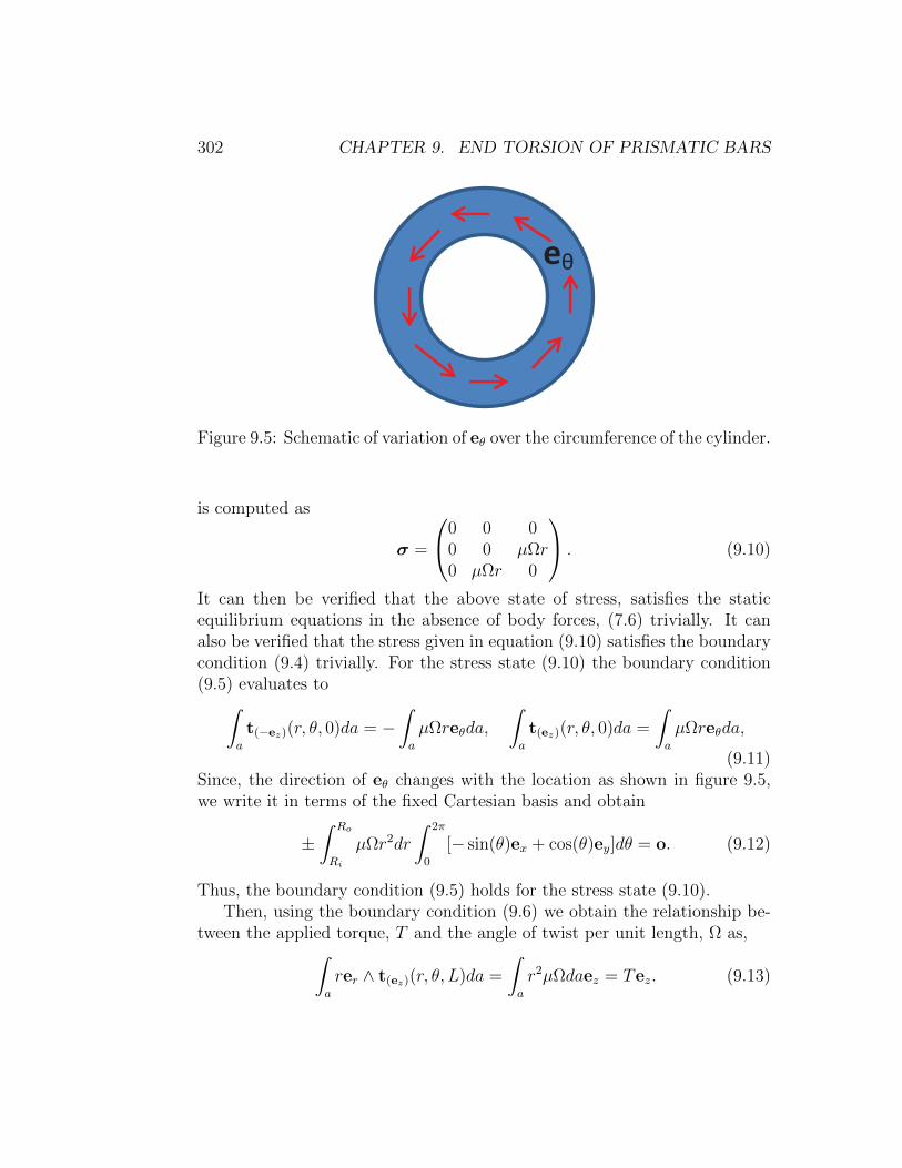
302 CHAPTER 9. END TORSION OF PRISMATIC BARS
eθ
Figure 9.5: Schematic of variation of eθ over the circumference of the cylinder.
is computed as
σ =
0 0 00 0 µΩr0 µΩr 0
. (9.10)
It can then be verified that the above state of stress, satisfies the staticequilibrium equations in the absence of body forces, (7.6) trivially. It canalso be verified that the stress given in equation (9.10) satisfies the boundarycondition (9.4) trivially. For the stress state (9.10) the boundary condition(9.5) evaluates to∫
a
t(−ez)(r, θ, 0)da = −∫a
µΩreθda,
∫a
t(ez)(r, θ, 0)da =
∫a
µΩreθda,
(9.11)Since, the direction of eθ changes with the location as shown in figure 9.5,we write it in terms of the fixed Cartesian basis and obtain
±∫ Ro
Ri
µΩr2dr
∫ 2π
0
[− sin(θ)ex + cos(θ)ey]dθ = o. (9.12)
Thus, the boundary condition (9.5) holds for the stress state (9.10).Then, using the boundary condition (9.6) we obtain the relationship be-
tween the applied torque, T and the angle of twist per unit length, Ω as,∫a
rer ∧ t(ez)(r, θ, L)da =
∫a
r2µΩdaez = Tez. (9.13)
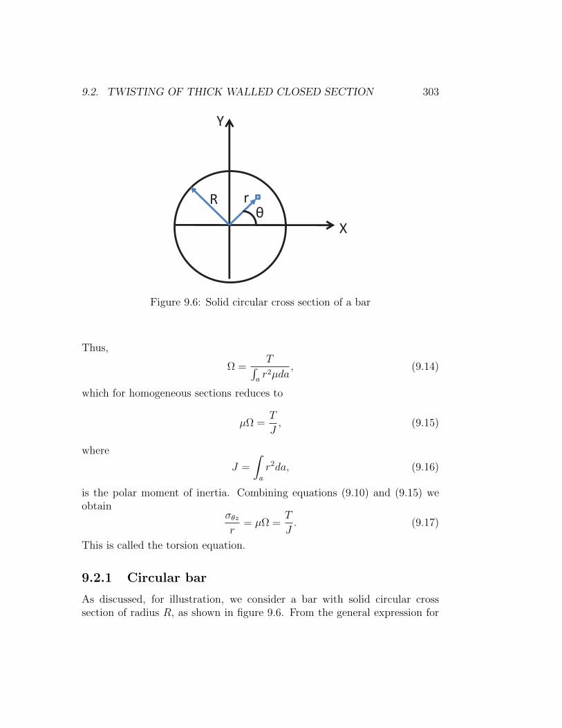
9.2. TWISTING OF THICK WALLED CLOSED SECTION 303
θ r R
X
Y
Figure 9.6: Solid circular cross section of a bar
Thus,
Ω =T∫
ar2µda
, (9.14)
which for homogeneous sections reduces to
µΩ =T
J, (9.15)
where
J =
∫a
r2da, (9.16)
is the polar moment of inertia. Combining equations (9.10) and (9.15) weobtain
σθzr
= µΩ =T
J. (9.17)
This is called the torsion equation.
9.2.1 Circular bar
As discussed, for illustration, we consider a bar with solid circular crosssection of radius R, as shown in figure 9.6. From the general expression for
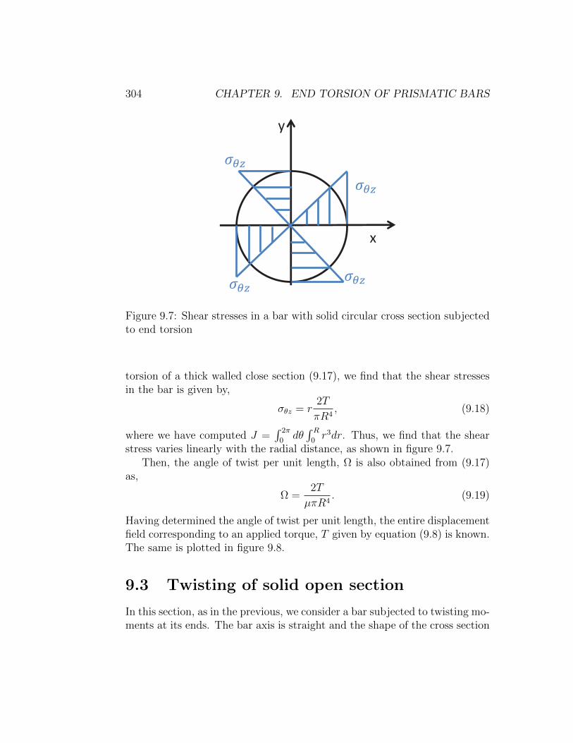
304 CHAPTER 9. END TORSION OF PRISMATIC BARS
x
y
Figure 9.7: Shear stresses in a bar with solid circular cross section subjectedto end torsion
torsion of a thick walled close section (9.17), we find that the shear stressesin the bar is given by,
σθz = r2T
πR4, (9.18)
where we have computed J =∫ 2π
0dθ∫ R
0r3dr. Thus, we find that the shear
stress varies linearly with the radial distance, as shown in figure 9.7.Then, the angle of twist per unit length, Ω is also obtained from (9.17)
as,
Ω =2T
µπR4. (9.19)
Having determined the angle of twist per unit length, the entire displacementfield corresponding to an applied torque, T given by equation (9.8) is known.The same is plotted in figure 9.8.
9.3 Twisting of solid open section
In this section, as in the previous, we consider a bar subjected to twisting mo-ments at its ends. The bar axis is straight and the shape of the cross section

9.3. TWISTING OF SOLID OPEN SECTION 305
(a) Undeformed circular bar (b) Deformed circular bar
Figure 9.8: Deformation of a bar with circular cross section subjected to endtorsion
is constant along the axis. The bar is assumed to have a solid cross section,i.e, a simply connected domain. A domain is said to be simply connected ifany closed curve in the domain can be shrunk to a point in the domain itself,without leaving the domain. A domain which is not simply connected is saidto be multiply connected. We shall analyze multiply connected domains inthe next section.
Though the problem formulation does not assume any specific shape forthe cross section, the displacement and stress field obtained are cross sectionspecific. Let us assume that the boundary of the cross section is defined bya function, f(x, y) = 0. This function for a ellipse centered about the originand major and minor axis oriented about the ex and ey directions would be,f(x, y) = x2/a2 +y2/b2−1. Consequently, for the body is assumed to occupya region in Euclidean point space, defined by B = (x, y, z)|f(x, y) ≤ 0, 0 ≤Z ≤ L, where L is a constant. Here we are assuming that the bar is asolid cross section with the cross section having only one surface, f(x, y) =0 denoted by ∂A. To be more precise, the cross section is simply connected.Since, we are interested in the case where in the bar is subjected to pure end

306 CHAPTER 9. END TORSION OF PRISMATIC BARS
torsional moment, the traction boundary conditions are:
t(en)(∂A, z) = o, (9.20)∫a
t(−ez)(x, y, 0)da = o, (9.21)∫a
t(ez)(x, y, L)da = o, (9.22)∫a
(xex + yey) ∧ t(−ez)(z, y, 0)da = −Tez, (9.23)∫a
(xex + yey) ∧ t(ez)(x, y, L)da = Tez, (9.24)
where
en =[∂f∂y
ex − ∂f∂x
ey]√(∂f∂x
)2+(∂f∂y
)2, (9.25)
and T is a constant. Here en is obtained such that it is in the xy plane,perpendicular to grad(f) and is a unit vector. Recognize that grad(f) givesthe tangent vector to the cross section for any point in ∂A. The orientationof en and grad(f) is as shown in figure 9.9. Further, since one end of thisbody is assumed to be fixed against twisting but free to displace axially andthe other end free to displace in all directions, the displacement boundaryconditions for this problem is,
u(x, y, 0) = uz(x, y)ez, (9.26)
where uz is any function of x and y. Here we have assumed that the surfaceof the body defined by z = 0 is fixed against twisting but free to displaceaxially and the other surfaces are free to displace in all directions.
In a solid cross section, as a result of a twist, each cross section undergoesa rotational displacement about the z axis. For any two cross sections therelative angle of rotation is called the angle of twist between the two sections.Let ∆β be the angle of twist for two cross sections at distance ∆z and Ω bethe angle of twist per unit length of the bar, then
∆β = Ω(∆z). (9.27)
Since the conditions are same for all cross sections, the above equation appliesto any two cross sections at a distance ∆z along the bar length. Thus, Ω is

9.3. TWISTING OF SOLID OPEN SECTION 307
x
y = grad (f)
Figure 9.9: Boundary conditions at the surface of a bar subjected to endtorsion
a constant along the bar length. Also, since at z = 0, β = 0, by virtue ofthe surface defined by z = 0 being fixed against rotation, the angle of twist,β for a cross sections at distance z from the surface defined by z = 0 is
β = Ωz. (9.28)
Consider a cross section at a distance z from the fixed end. In thatsection consider a point A with coordinates (x, y, z). Assuming the origin ofthe coordinate system to be located at the axis of twisting, let r denote theradial distance of the point A from the origin and let θ denote the angle thatthis radial line makes with the ex, as shown in the figure 9.10. Let A moveto A′ due to twisting of the bar, as shown in the figure 9.10. The arc lengthAA′ would be equal to rβ, where β is the angle of twist at the cross sectionand is related to the angle of twist per unit length through (9.28). Hence,the arc length AA′ would be,
AA′ = rβ = rΩz. (9.29)
Since, the angle of twist β is small, we approximate the secant length, i.e.,the length of the straight line between AA′ with its arc length. Consequently,the x component of the displacement of A is given by,
ux = −AA′ sin(θ) = −AA′ sin(θ) = −rΩz sin(θ) = −Ωzy, (9.30)
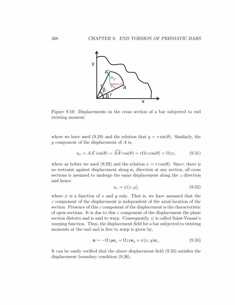
308 CHAPTER 9. END TORSION OF PRISMATIC BARS
A
A’
r β
βθ
x
y
r
Figure 9.10: Displacements in the cross section of a bar subjected to endtwisting moment
where we have used (9.29) and the relation that y = r sin(θ). Similarly, they component of the displacement of A is,
ux = AA′ cos(θ) = AA′ cos(θ) = rΩz cos(θ) = Ωzx, (9.31)
where as before we used (9.29) and the relation x = r cos(θ). Since, there isno restraint against displacement along ez direction at any section, all crosssections is assumed to undergo the same displacement along the z directionand hence
uz = ψ(x, y), (9.32)
where ψ is a function of x and y only. That is, we have assumed that thez component of the displacement is independent of the axial location of thesection. Presence of this z component of the displacement is the characteristicof open sections. It is due to this z component of the displacement the planesection distorts and is said to warp. Consequently, ψ is called Saint-Venant’swarping function. Thus, the displacement field for a bar subjected to twistingmoments at the end and is free to warp is given by,
u = −Ωzyex + Ωzxey + ψ(x, y)ez. (9.33)
It can be easily verified that the above displacement field (9.33) satisfies thedisplacement boundary condition (9.26).

9.3. TWISTING OF SOLID OPEN SECTION 309
Substituting equation (9.33) in the strain-displacement equation (7.1),the Cartesian components of the strain are computed to be
ε =
0 0 −Ωy + ∂ψ∂x
0 0 Ωx+ ∂ψ∂y
−Ωy + ∂ψ∂x
Ωx+ ∂ψ∂y
0
. (9.34)
For this state of strain, the corresponding Cartesian components of the stressare obtained from Hooke’s law (7.2) as
σ =
0 0 µ
(−Ωy + ∂ψ
∂x
)0 0 µ
(Ωx+ ∂ψ
∂y
)µ(−Ωy + ∂ψ
∂x
)µ(
Ωx+ ∂ψ∂y
)0
. (9.35)
For this stress state, (9.35) to be possible in a body in static equilibrium,without any body force acting on it, it should satisfy the balance of linearmomentum equations (7.6) which requires that,
∂2ψ
∂x2+∂2ψ
∂y2= 0. (9.36)
Now, we have to find ψ such that equation (9.36) holds along with the pre-scribed traction boundary conditions (9.20) through (9.24).
Boundary condition (9.20) requires
µ
[−Ωy +
∂ψ
∂x
]∂f
∂y− µ
[Ωx+
∂ψ
∂y
]∂f
∂x= 0, (9.37)
for (x, y) ∈ ∂A. Both the boundary conditions (9.21) and (9.22) yield thefollowing restriction on ψ,∫
a
µ
[−Ωy +
∂ψ
∂x
]da = 0,
∫a
µ
[Ωx+
∂ψ
∂y
]da = 0, (9.38)
On assuming that the bar is homogeneous and appealing to Green’s theorem(section 2.9.3), equation (9.38) reduces to,∫
a
µ
[−Ωy +
∂ψ
∂x
]da = −µΩycA+
∮c
ψ
∂f∂y√(
∂f∂x
)2+(∂f∂y
)2ds = 0, (9.39)
∫a
µ
[Ωx+
∂ψ
∂y
]da = µΩxcA−
∮c
ψ∂f∂x√(
∂f∂x
)2+(∂f∂y
)2ds = 0, (9.40)

310 CHAPTER 9. END TORSION OF PRISMATIC BARS
where (xc, yc) is the coordinates of the centroid of the cross section. Onassuming that the axis of twisting coincides with the centroid and furtherrequiring that the origin of the coordinate system coincide with the centroidof the cross section, equations (9.39) and (9.40) requires,∮
c
ψ∂f
∂yds = 0,
∮c
ψ∂f
∂xds = 0. (9.41)
Finally, the boundary conditions (9.23) and (9.24) require that∫a
(xσyz−yσxz)da =
∫a
µΩ(x2 +y2)da+
∫a
µ
(x∂ψ
∂y− y∂ψ
∂x
)da = T. (9.42)
Recognizing that∫a(x2 + y2)da = J , polar moment of inertia equation (9.42)
can be simplified as,
T = µΩJ + µ
∫a
(x∂ψ
∂y− y∂ψ
∂x
)da, (9.43)
where we have used the assumption already made that the bar is homoge-
neous. For many cross sections,∫a
(x∂ψ∂y− y ∂ψ
∂x
)da < 0. Thus, the torsional
stiffness1 which would be µJ , in the absence of warping (i.e., ψ = 0), de-creases due to warping (i.e., when ψ 6= 0). Hence, warping is said to decreasethe torsional stiffness of the cross section. Equation (9.43) is used find Ω.
Experience has shown that it is difficult to find ψ that satisfies the gov-erning equation (9.36) along with the boundary conditions (9.37) and (9.41).Hence, we recast the problem using Prandtl stress function.
Stress function formulation
Defining a differentiable function, φ = φ(x, y) called the Prandtl stress func-tion, we relate the components of the stress to this stress function as,
σ =
0 0 ∂φ∂y
0 0 −∂φ∂x
∂φ∂y−∂φ∂x
0
, (9.44)
1Torsional stiffness is defined as the torque required to cause a unit angle of twist perunit length.

9.3. TWISTING OF SOLID OPEN SECTION 311
so that the equilibrium equations (7.6) are satisfied for any choice of φ.Now, one can proceed in one of two ways. Follow the standard approach
and find the strain corresponding to the stress state (9.44), substitute thesame in the compatibility conditions and find the governing equation thatφ should satisfy. Here we obtain the same governing equation through analternate approach.
Equating the stress states (9.35) and (9.44) as it represents for the sameboundary value problem, we obtain
∂φ
∂y= µ
[−Ωy +
∂ψ
∂x
], (9.45)
∂φ
∂x= −µ
[Ωx+
∂ψ
∂y
]. (9.46)
Differentiating equation (9.45) with respect to y and equation (9.46) withrespect to x and adding the resulting equations, we obtain
∂2φ
∂x2+∂2φ
∂y2= −2µΩ, (9.47)
where we have made use of the requirement that ∂2ψ∂x∂y
= ∂2ψ∂y∂x
. By virtue of
the stress function being smooth enough so that ∂2φ∂x∂y
= ∂2φ∂y∂x
, the governing
equation for ψ (9.36) is trivially satisfied.The boundary condition given in equation (9.37) in terms of the warping
function, ψ is rewritten in terms of the Prandtl stress function, φ usingequations (9.45) and (9.46) as,
∂φ
∂y
∂f
∂y+∂φ
∂x
∂f
∂x= grad(φ) · grad(f) = 0, (9.48)
for (x, y) ∈ ∂A. Since, grad(f) 6= o and its direction changes with thelocation on the boundary of the cross section, grad(φ) = o on the boundaryof the cross section. This implies that
φ(x, y) = C0, for (x, y) ∈ ∂A, (9.49)
where C0 is a constant. Since, the stress and displacement fields dependonly in the derivative of the stress potential and not its value at a location, it

312 CHAPTER 9. END TORSION OF PRISMATIC BARS
suffices to find this stress function up to a constant2. Therefore, we arbitrarilyset C0 = 0, understanding that it can take any value and that the stress anddisplacement field would not change because of this. Hence, equation (9.49)reduces to requiring,
φ(x, y) = 0, for (x, y) ∈ ∂A. (9.50)
The boundary condition (9.21) and (9.22) for the stress state (9.44) re-quire ∫
a
∂φ
∂yda = 0,
∫a
∂φ
∂xda = 0. (9.51)
Appealing to Green’s theorem for simply connected domains, the above equa-tion (9.51) reduces to∫
a
∂φ
∂yda =
∮c
φ∂f
∂xds = C0
∮c
∂f
∂xds = 0, (9.52)∫
a
∂φ
∂xda =
∮c
φ∂f
∂yds = C0
∮c
∂f
∂yds = 0, (9.53)
where we have used (9.49) and the fact that∮c∂f∂xds = 0 and
∮c∂f∂yds = 0 for
closed curves.Finally, the boundary conditions (9.23) and (9.24) for the stress state
(9.44) yields,
−∫a
[x∂φ
∂x+ y
∂φ
∂y
]da = T. (9.54)
Noting that∫a
x∂φ
∂x=
∫a
[∂(xφ)
∂x− φ]da =
∮c
xφ∂f
∂yds−
∫a
φda = −∫a
φda, (9.55)∫a
y∂φ
∂y=
∫a
[∂(yφ)
∂y− φ]da =
∮c
yφ∂f
∂xds−
∫a
φda = −∫a
φda, (9.56)
where we have used the Green’s theorem for simply connected domain andequation (9.50). Substituting the above equations in (9.54) we obtain,
T = 2
∫a
φda. (9.57)
2This means that if φ is a stress function for the given boundary value problem thenφ+C0, where C0 is some constant, will also be an admissible stress function for the sameboundary value problem.

9.3. TWISTING OF SOLID OPEN SECTION 313
Thus, we have to find φ such that the governing equation (9.47) has tohold along with the boundary condition (9.50). Then, we use equation (9.57)to find the torsional moment required to realize a given angle of twist perunit length Ω.
Membrane analogy
The governing equation (9.47) along with the boundary condition (9.50) and(9.57) is identical with those governing the static deflection under uniformpressure of an elastic membrane in the same shape as that of the membersubjected to torsion. This fact creates an analogy between the torsion prob-lem and elastic membrane under uniform pressure. This analogy is exploitedto get the qualitative features that the stress function should posses and thisaids in developing approximate solutions. Obtaining the governing equationfor the static deflection of an elastic membrane under uniform pressure andshowing that it is identical to (9.47) is beyond the scope of this lecture notes.One may refer Sadd [4] for the same.
In the following three sections, we apply the above general framework tosolve problems of bars with specific cross section shapes subjected to endtorsion.
9.3.1 Solid elliptical section
The first cross section shape that we consider is that of an ellipse. That iswe study a bar with elliptical cross section, whose boundary is defined bythe function,
f(x, y) =x2
a2+y2
b2− 1 = 0, (9.58)
where a and b are constants and we have assumed that the major and minoraxis of the ellipse coincides with the coordinate basis, as shown in the figure9.11.
Choosing the Prandtl stress function to be,
φ = C
[x2
a2+y2
b2− 1
], (9.59)
where C is a constant, we find that it satisfies the boundary condition (9.50).
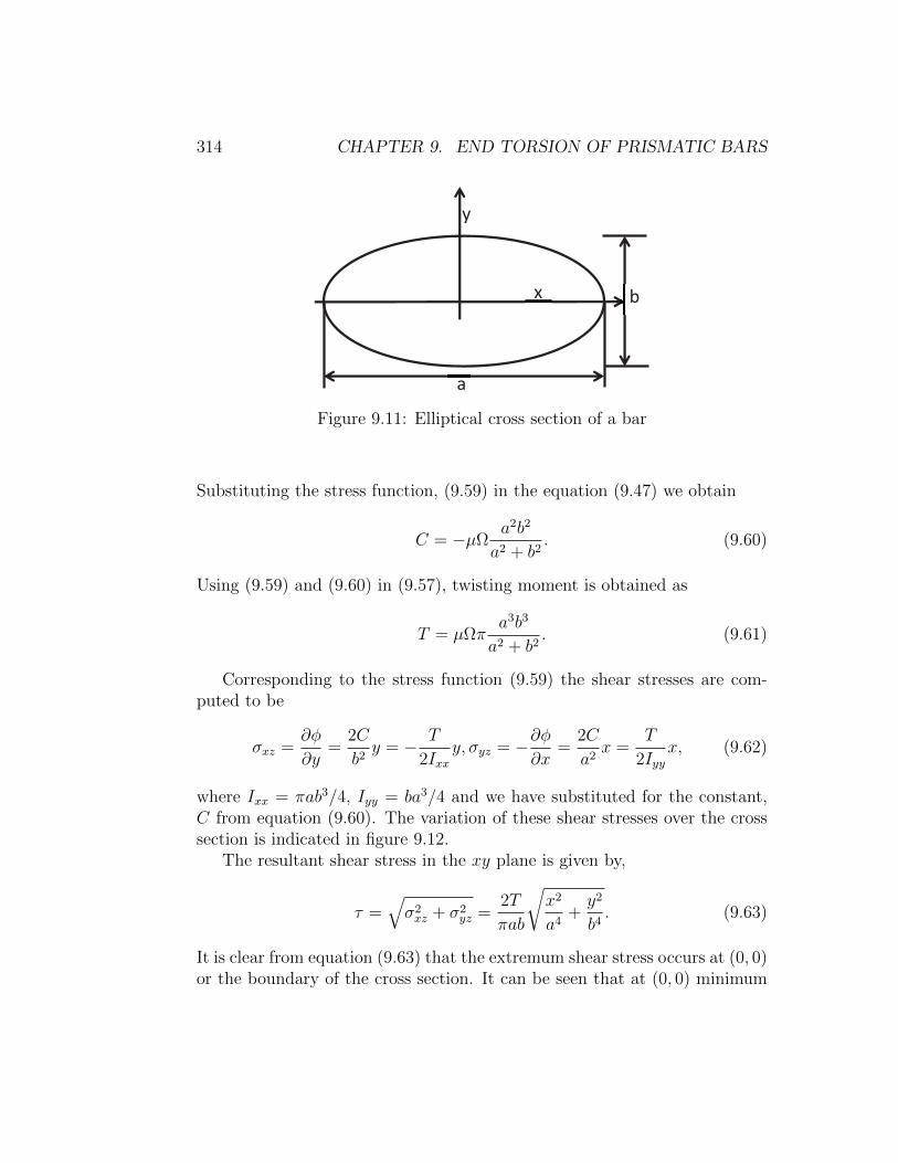
314 CHAPTER 9. END TORSION OF PRISMATIC BARS
x b
a
y
Figure 9.11: Elliptical cross section of a bar
Substituting the stress function, (9.59) in the equation (9.47) we obtain
C = −µΩa2b2
a2 + b2. (9.60)
Using (9.59) and (9.60) in (9.57), twisting moment is obtained as
T = µΩπa3b3
a2 + b2. (9.61)
Corresponding to the stress function (9.59) the shear stresses are com-puted to be
σxz =∂φ
∂y=
2C
b2y = − T
2Ixxy, σyz = −∂φ
∂x=
2C
a2x =
T
2Iyyx, (9.62)
where Ixx = πab3/4, Iyy = ba3/4 and we have substituted for the constant,C from equation (9.60). The variation of these shear stresses over the crosssection is indicated in figure 9.12.
The resultant shear stress in the xy plane is given by,
τ =√σ2xz + σ2
yz =2T
πab
√x2
a4+y2
b4. (9.63)
It is clear from equation (9.63) that the extremum shear stress occurs at (0, 0)or the boundary of the cross section. It can be seen that at (0, 0) minimum

9.3. TWISTING OF SOLID OPEN SECTION 315
x
a
y
b
Figure 9.12: Shear stresses in a bar with elliptical cross section subjected toend torsion
shear stress occurs, as τ = 0 at this location. At the boundary the extremumshear stresses would occur at (0,±b) and (±a, 0). Thus, the extremum shearstresses are τext = 2T/(πab2) at (0,±b) and τext = 2T/(πba2) at (±a, 0). Ifa > b, then the maximum shear stress in the elliptical cross section is,
τmax =2T
πab2. (9.64)
Substituting (9.59) in equations (9.45) and (9.46) and rearranging weobtain
∂ψ
∂x= Ωy +
2C
µb2y,
∂ψ
∂y= −
[Ωx+
2C
µa2x
]. (9.65)
Solving the differential equations (9.65) we obtain
ψ(x, y) = Tb2 − a2
πa3b3µxy +D0, (9.66)
where D0 is a constant. Since, there is no rigid body translation, we requirethat ψ(0, 0) = 0. Hence, D0 = 0. Thus, we find that the section warps intoa diagonally symmetric surface as shown in figure 9.13.
Rearranging the equation (9.61) we can get Ω as a function of torque, Tas
Ω =T [a2 + b2]
µπa3b3(9.67)
The entire displacement field, (9.33) for a bar with elliptical cross section isnow known that we have found the warping function (9.66). The deformation
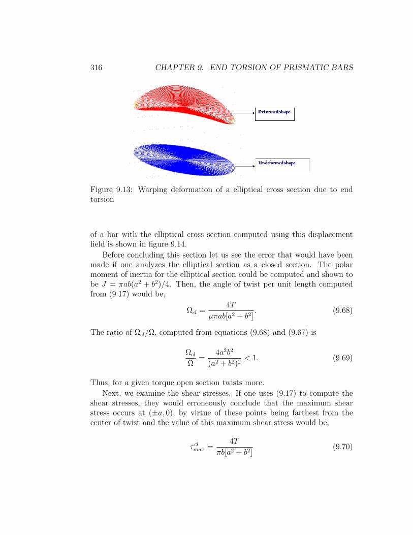
316 CHAPTER 9. END TORSION OF PRISMATIC BARS
Figure 9.13: Warping deformation of a elliptical cross section due to endtorsion
of a bar with the elliptical cross section computed using this displacementfield is shown in figure 9.14.
Before concluding this section let us see the error that would have beenmade if one analyzes the elliptical section as a closed section. The polarmoment of inertia for the elliptical section could be computed and shown tobe J = πab(a2 + b2)/4. Then, the angle of twist per unit length computedfrom (9.17) would be,
Ωcl =4T
µπab[a2 + b2]. (9.68)
The ratio of Ωcl/Ω, computed from equations (9.68) and (9.67) is
Ωcl
Ω=
4a2b2
(a2 + b2)2< 1. (9.69)
Thus, for a given torque open section twists more.
Next, we examine the shear stresses. If one uses (9.17) to compute theshear stresses, they would erroneously conclude that the maximum shearstress occurs at (±a, 0), by virtue of these points being farthest from thecenter of twist and the value of this maximum shear stress would be,
τ clmax =4T
πb[a2 + b2](9.70)
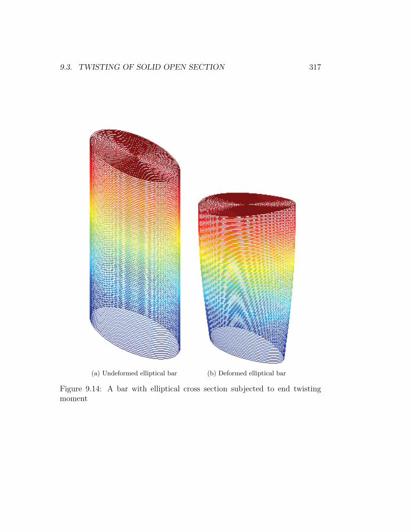
9.3. TWISTING OF SOLID OPEN SECTION 317
(a) Undeformed elliptical bar (b) Deformed elliptical bar
Figure 9.14: A bar with elliptical cross section subjected to end twistingmoment
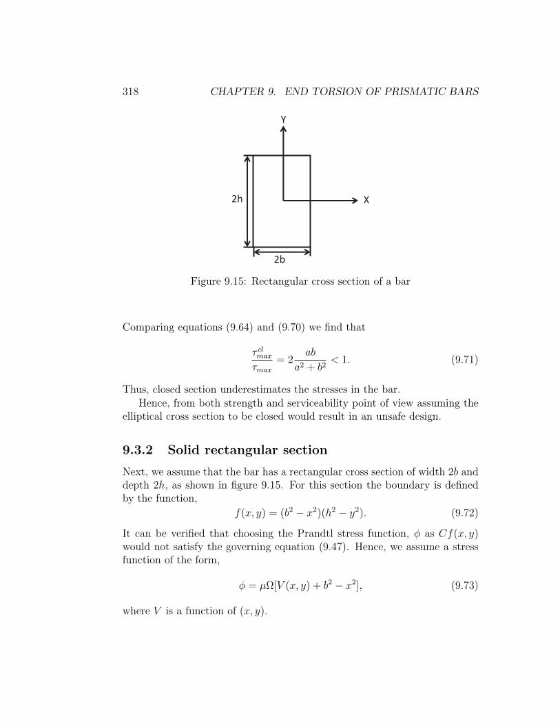
318 CHAPTER 9. END TORSION OF PRISMATIC BARS
X
Y
2h
2b
Figure 9.15: Rectangular cross section of a bar
Comparing equations (9.64) and (9.70) we find that
τ clmaxτmax
= 2ab
a2 + b2< 1. (9.71)
Thus, closed section underestimates the stresses in the bar.Hence, from both strength and serviceability point of view assuming the
elliptical cross section to be closed would result in an unsafe design.
9.3.2 Solid rectangular section
Next, we assume that the bar has a rectangular cross section of width 2b anddepth 2h, as shown in figure 9.15. For this section the boundary is definedby the function,
f(x, y) = (b2 − x2)(h2 − y2). (9.72)
It can be verified that choosing the Prandtl stress function, φ as Cf(x, y)would not satisfy the governing equation (9.47). Hence, we assume a stressfunction of the form,
φ = µΩ[V (x, y) + b2 − x2], (9.73)
where V is a function of (x, y).

9.3. TWISTING OF SOLID OPEN SECTION 319
Substituting equation (9.73) in equation (9.47) and simplifying we obtain,
∂2V
∂x2+∂2V
∂y2= 0. (9.74)
Then, the boundary condition (9.50) requires that
V (±b, y) = 0, V (x,±h) = x2 − b2. (9.75)
Thus, we need to solve the differential equation (9.74) subject to the bound-ary condition (9.75).
Towards this, we seek solution of the form
V = Vx(x)Vy(y), (9.76)
where Vx is a function of x and Vy is a function of y alone. Substitutingthe assumed special form for V , (9.76) in equation (9.74) and simplifying weobtain,
1
Vx
d2Vxdx2
= − 1
Vy
d2Vydy2
= k2, (9.77)
where k is any constant. Recognize that the left hand side of the equationis a function of x alone and the right hand side is a function of y alone.Hence, for these functions to be same, they have to be a constant. Solvingthe second order ordinary differential equations (9.77) we obtain,
Vx = A cos(kx) +B sin(kx), Vy = C cosh(ky) +D sinh(ky). (9.78)
Consistent with the boundary condition (9.75), we expect the functions Vxand Vy to be even functions, i.e., Vx(−x) = Vx(x) and Vy(−y) = Vy(y). Hence,
B = D = 0. (9.79)
Substituting (9.79) in the equation (9.78) and the result into equation (9.76)we obtain,
V = AC cos(kx) cosh(ky) = E cos(kx) cosh(ky), (9.80)
where E is some arbitrary constant. The equation (9.80) on applying theboundary condition (9.75a), i.e., V (±b, y) = 0 yields that
k =(2n+ 1)π
2b, (9.81)

320 CHAPTER 9. END TORSION OF PRISMATIC BARS
where n is any integer. Since, the governing equation for V , (9.74) is aLaplace equation, it is a linear equation. Consequently, if two functionssatisfy the given equation (9.74) then a linear combination of these functionsalso satisfies the Laplace equation. So the solution (9.80) can be written as,
V =∞∑n=1
En cos
((2n+ 1)π
2bx
)cosh
((2n+ 1)π
2by
), (9.82)
where En’s are constant. Substituting (9.82) in the boundary condition(9.75b), i.e., V (x,±h) = x2 − h2 we obtain,
∞∑n=1
En cosh
((2n+ 1)πh
2b
)cos
((2n+ 1)πx
2b
)= x2 − b2. (9.83)
Now, we have to find the constants En such that for −b ≤ x ≤ b, a linearcombination of cosines approximates the quadratic function on the right handside of equation (9.83). Using the standard techniques in fourier analysis weobtain,
En cosh
((2n+ 1)πh
2b
)=
∫ b
−b[x2 − b2] cos
((2n+ 1)πx
2b
). (9.84)
Integrating the above equation and rearranging, we obtain
En =32b2(−1)n
(2n+ 1)3π3 cosh(
(2n+1)πh2b
) . (9.85)
Substituting equation (9.85) in (9.82) and the resulting equation in (9.73),we obtain
φ = µΩ
(b2 − x2) +32b2
π3
∞∑n=0
(−1)n cos(
(2n+1)πx2b
)cosh
((2n+1)πy
2b
)(2n+ 1)3 cosh
((2n+1)πh
2b
) .(9.86)
Having found the stress function, we are now in a position to find the shearstresses and the warping function. First, we compute the stresses as,
σxz =∂φ
∂y
= µΩ32b2
π3
∞∑n=0
(−1)n cos(
(2n+1)πx2b
) [(2n+1)π
2b
]sinh
((2n+1)πy
2b
)(2n+ 1)3 cosh
((2n+1)πh
2b
) , (9.87)

9.3. TWISTING OF SOLID OPEN SECTION 321
2b
2h x
y
Figure 9.16: Schematic of shear stress distribution in a bar with solid rect-angular cross section subjected to end torsion
σyz = −∂φ∂x
= µΩ
2x+32b2
π3
∞∑n=0
(−1)n sin(
(2n+1)πx2b
) [(2n+1)π
2b
]cosh
((2n+1)πy
2b
)(2n+ 1)3 cosh
((2n+1)πh
2b
) .
(9.88)
Figure 9.16 schematically shows the shear stress distribution in a rectan-gular cross section along the sides of the rectangle and along the lines x = 0and y = 0. The shear stress is maximum on the boundary and zero at thecenter of the rectangle. The maximum shear stress occurs at the middle ofthe long side and is given by,
τmax = σyz(±b, 0) = µΩ
2b+32b
π2
∞∑n=0
(−1)n
(2n+ 1)2 cosh(
(2n+1)πh2b
) , (9.89)
where we have assumed that h ≥ b.
Substituting (9.87) in equation (9.45) and solving the first order ordinary

322 CHAPTER 9. END TORSION OF PRISMATIC BARS
Figure 9.17: Warping deformation of a rectangular section due to end torsion
differential equation for ψ we obtain
ψ = −Ω32b2
π3
∞∑n=0
(−1)n sin(
(2n+1)πx2b
)sinh
((2n+1)πy
2b
)(2n+ 1)3 cosh
((2n+1)πh
2b
) + Ωxy + g(y). (9.90)
Substituting equations (9.88) and (9.90) in equation (9.46) and solving thefirst order ordinary differential equation for g we obtain g(y) = D0, a con-stant. Since, the bar does not move as a rigid body, we want ψ(0, 0) = 0.Hence, D0 = 0. Consequently, the warping function is,
ψ = −Ω32b2
π3
∞∑n=0
(−1)n sin(
(2n+1)πx2b
)sinh
((2n+1)πy
2b
)(2n+ 1)3 cosh
((2n+1)πh
2b
) + Ωxy. (9.91)
Figure 9.17 plots the warped rectangular section.Substituting (9.87) and (9.88) in equation (9.57) we can relate the applied
torque, T to the realized angle of twist per unit length, Ω as
T =16µΩb3h
3− 1024µΩb4
π5
∞∑n=0
1
(2n+ 1)5tanh
((2n+ 1)πh
2b
)(9.92)
This relation is expressed as
T = µΩC1(2h)(2b)3, (9.93)
where C1 is a non-dimensional parameter which depends on h/b. In thesame spirit, the maximum shear stress, (9.89) could be related to the applied

9.3. TWISTING OF SOLID OPEN SECTION 323
Table 9.1: Tabulation of parameters C1 and C2 as a function of h/b
h/b C1 C2
1 0.141 4.801.5 0.196 4.332.0 0.229 4.063.0 0.263 3.744.0 0.281 3.546 0.299 3.3410 0.312 3.21∞ 0.333 3.00
torque as,
τmax = C2T
(2h)(2b)2. (9.94)
where C2 is another non-dimensional parameter which depends on h/b. Val-ues of C1 and C2 for various h/b ratios are tabulated in table 9.1.
Thus, for thin rectangular sections, when h/b tends to ∞,
T = µΩwt3
3, τmax =
3T
wt2, (9.95)
where we have assumed the section to have a thickness, t = 2b and depth, w= 2h. It should be mentioned that irrespective of the orientation of the thinrectangular section, the equation (9.95) remains the same. This is because ofthe requirement that h ≥ b. Physically, irrespective of the orientation of thesection, the torsion is resisted by the spatial variation of the shear stressesthrough the thickness of the section as shown in figure 9.19.
9.3.3 Thin rolled section
Here we study the problem of end torsion of a bar whose cross section isnarrow and has small curvature such as those shown in figure 9.20. Suchsections are usually made of hot rolled steel and hence are called rolled sec-tions. Since, the shape across the thickness is similar to that of the thinrectangular section, excepting at the bent corners, it is assumed that the

324 CHAPTER 9. END TORSION OF PRISMATIC BARS
(a) Undeformed rectangular bar (b) Deformed rectangular bar
Figure 9.18: A bar with rectangular cross section subjected to end twistingmoment

9.3. TWISTING OF SOLID OPEN SECTION 325
y
x t
w
τ
(a) Thin rectangular section oriented along x direction
y
x
t
w τ
(b) Thin rectan-gular section ori-ented along y di-rection
Figure 9.19: Schematic of shear stress distribution in a thin rectangularsection in different orientations

326 CHAPTER 9. END TORSION OF PRISMATIC BARS
t
t
b1 b2
τ
(a) Angle section
tw
tf
tf
h
b
b
(b) I section
Figure 9.20: Schematic of shear stress distribution in a thin rolled sections
solution obtained for thin rectangular section holds. In order for the cornersnot to change the displacement and stress field from that obtained for a thinrectangular section, it is required that the radius of curvature of these cornersbe large.
Thus, for the angle section shown in figure 9.20a, the torque required torealize a given angle of twist per unit length and the maximum shear stressin the section is obtained from (9.95) as
T = µΩt3(b1 + b2)
3, τmax =
3T
(b1 + b2)t2, (9.96)
where we have treated the entire angle without the 90 degree bend, as a thinwalled rectangular section. In order for the above equations to be reasonable,(b1 + b2)/t > 10 and the radius of the curvature of the bent corner large.
Similarly, for the I section shown in figure 9.20b, the torque required torealize a given angle of twist per unit length and the maximum shear stressin the section is obtained from (9.95) as
T = µΩ2t3fb1 + t3wh
3, τmax =
3T
2t2fb1 + t2wh, (9.97)
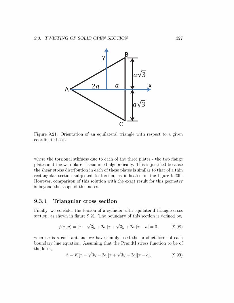
9.3. TWISTING OF SOLID OPEN SECTION 327
y
x
A
B
C Figure 9.21: Orientation of an equilateral triangle with respect to a givencoordinate basis
where the torsional stiffness due to each of the three plates - the two flangeplates and the web plate - is summed algebraically. This is justified becausethe shear stress distribution in each of these plates is similar to that of a thinrectangular section subjected to torsion, as indicated in the figure 9.20b.However, comparison of this solution with the exact result for this geometryis beyond the scope of this notes.
9.3.4 Triangular cross section
Finally, we consider the torsion of a cylinder with equilateral triangle crosssection, as shown in figure 9.21. The boundary of this section is defined by,
f(x, y) = [x−√
3y + 2a][x+√
3y + 2a][x− a] = 0, (9.98)
where a is a constant and we have simply used the product form of eachboundary line equation. Assuming that the Prandtl stress function to be ofthe form,
φ = K[x−√
3y + 2a][x+√
3y + 2a][x− a], (9.99)
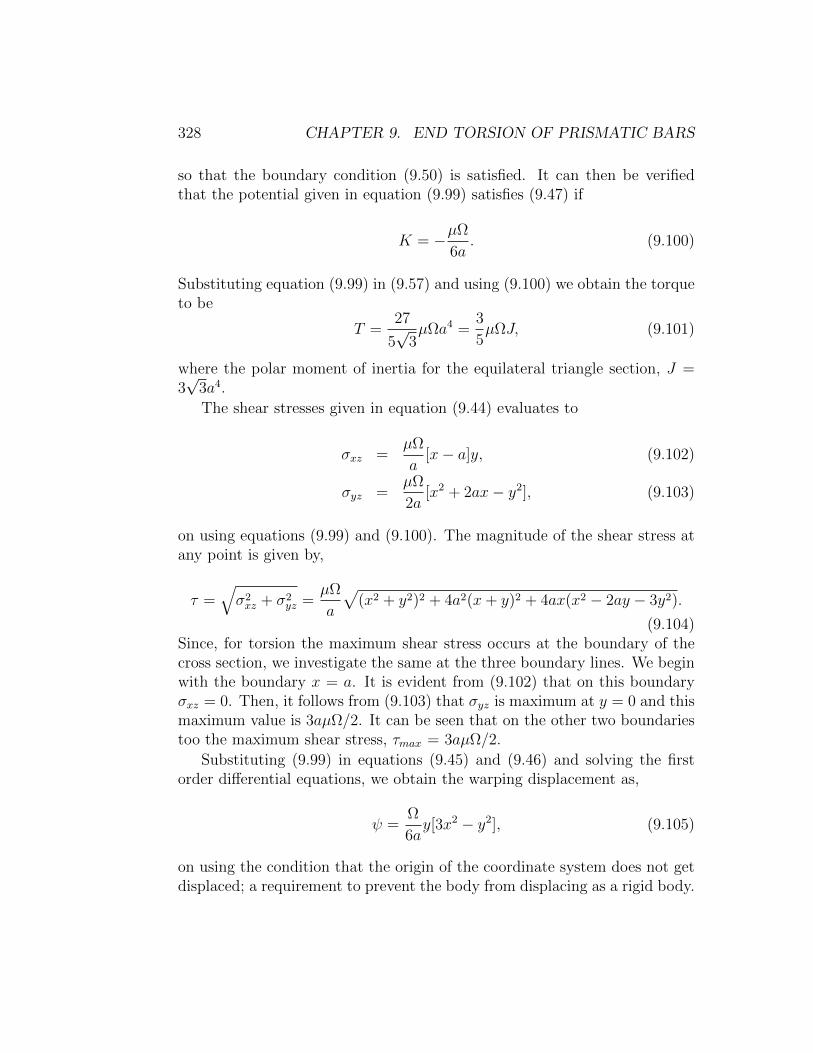
328 CHAPTER 9. END TORSION OF PRISMATIC BARS
so that the boundary condition (9.50) is satisfied. It can then be verifiedthat the potential given in equation (9.99) satisfies (9.47) if
K = −µΩ
6a. (9.100)
Substituting equation (9.99) in (9.57) and using (9.100) we obtain the torqueto be
T =27
5√
3µΩa4 =
3
5µΩJ, (9.101)
where the polar moment of inertia for the equilateral triangle section, J =3√
3a4.
The shear stresses given in equation (9.44) evaluates to
σxz =µΩ
a[x− a]y, (9.102)
σyz =µΩ
2a[x2 + 2ax− y2], (9.103)
on using equations (9.99) and (9.100). The magnitude of the shear stress atany point is given by,
τ =√σ2xz + σ2
yz =µΩ
a
√(x2 + y2)2 + 4a2(x+ y)2 + 4ax(x2 − 2ay − 3y2).
(9.104)Since, for torsion the maximum shear stress occurs at the boundary of thecross section, we investigate the same at the three boundary lines. We beginwith the boundary x = a. It is evident from (9.102) that on this boundaryσxz = 0. Then, it follows from (9.103) that σyz is maximum at y = 0 and thismaximum value is 3aµΩ/2. It can be seen that on the other two boundariestoo the maximum shear stress, τmax = 3aµΩ/2.
Substituting (9.99) in equations (9.45) and (9.46) and solving the firstorder differential equations, we obtain the warping displacement as,
ψ =Ω
6ay[3x2 − y2], (9.105)
on using the condition that the origin of the coordinate system does not getdisplaced; a requirement to prevent the body from displacing as a rigid body.
9.4. TWISTING OF HOLLOW SECTION 329
y
x xo xo
b
a
r r
Figure 9.22: Example of a multiply connected cross section. Elliptical crosssection with two circular holes.
9.4 Twisting of hollow section
In this section, as in the previous, we consider a bar subjected to twistingmoments at its ends. The bar axis is straight and the shape of the crosssection is constant along the axis. The bar is assumed to have a hollow crosssection, i.e, a multiply connected domain. That is any closed curves in thecross section cannot be shrunk to a point in the domain itself without leavingthe domain.
Let us assume that the boundary of the cross section is defined by afunction, f(x, y) = 0, the set of points constituting this boundary by ∂Ao,and the enclosed area by Ao. The boundary of the ith void in the interiorof the cross section is defined by the function gi(x, y) = 0, the set of pointsconstituting this boundary of the ith void by ∂Ai and the area enclosed bythe void, Ai. Thus, the area of the cross section, Acs is given by
Acs = Ao −N∑i=1
Ai, (9.106)
where we have assumed that there are N voids.Thus, for the cross section shown in figure 9.22, with the boundary of
the cross section in the form of an ellipse centered about origin and orientedsuch that the major and minor axis coincides with the ex and ey directions

330 CHAPTER 9. END TORSION OF PRISMATIC BARS
respectively and having two circular shaped voids of radius, r centered at(±xo, 0), the functions f(x, y) and gi(x, y) would be: f(x, y) = x2/a2+y2/b2−1, g1(x, y) = (x−xo)2+y2−r2 and g2(x, y) = (x+xo)
2+y2−r2. Consequently,this body is assumed to occupy a region in Euclidean point space, defined byB = (x, y, z)|f(x, y) ≤ 0, 0 ≤ Z ≤ L − (x, y, z)|f(x, y) ≤ 0, 0 ≤ Z ≤ L− (x, y, z)|f(x, y) ≤ 0, 0 ≤ Z ≤ L − (x, y, z)|g1(x, y) ≤ 0, 0 ≤ Z ≤ L− (x, y, z)|f(x, y) ≤ 0, 0 ≤ Z ≤ L − (x, y, z)|g2(x, y) ≤ 0, 0 ≤ Z ≤ L,where L is a constant.
Since, we are interested in the case where in the bar is subjected to pureend torsional moment, the traction boundary conditions are:
t(en)(∂Ao, z) = o, (9.107)
t(emi )(∂Ai, z) = o, (9.108)∫
a
t(−ez)(x, y, 0)da = o, (9.109)∫a
t(ez)(x, y, L)da = o, (9.110)∫a
(xex + yey) ∧ t(−ez)(z, y, 0)da = −Tez, (9.111)∫a
(xex + yey) ∧ t(ez)(x, y, L)da = Tez, (9.112)
where
en =[∂f∂y
ex − ∂f∂x
ey]√(∂f∂x
)2+(∂f∂y
)2, emi =
[∂gi∂y
ex − ∂gi∂x
ey]√(∂gi∂x
)2+(∂gi∂y
)2, (9.113)
and T is a constant. Here en is obtained such that it is in the xy plane,perpendicular to grad(f) and is a unit vector. Similarly, emi is obtainedsuch that it is in the xy plane, perpendicular to grad(gi) and is a unit vector.Recognize that grad(f) gives the tangent vector to the cross section for anypoint in ∂Ao and grad(gi) is the tangent vector to the cross section at anypoint in ∂Ai. Further, since one end of this body is assumed to be fixedagainst twisting but free to displace axially and the other end free to displacein all directions, the displacement boundary conditions for this problem is,
u(x, y, 0) = uz(x, y)ez, (9.114)

9.4. TWISTING OF HOLLOW SECTION 331
where uz is any function of x and y. Here we have assumed that the surfaceof the body defined by z = 0 is fixed against twisting but free to displaceaxially and the other surfaces are free to displace in all directions.
Thus, we find that the boundary value problem is similar to that in theprevious section (section 9.3) except for the additional boundary condition(9.108). Hence, we assume that the stress is as given in equation (9.44), interms of the Prandtl stress function, φ = φ(x, y). Following the standardprocedure, as outlined in section 9.3, it can be shown that the stress functionshould satisfy,
∂2φ
∂x2+∂2φ
∂y2= −2µΩ, (9.115)
where µ is the shear modulus, and Ω is the angle of twist per unit length.
For the assumed stress state, (9.44), the boundary condition (9.107) re-quires that grad(φ) · grad(f) = 0 on ∂Ao. Thus,
φ(x, y) = C0, for (x, y) ∈ ∂Ao, (9.116)
where C0 is a constant. As before, since, the stress and displacement fieldsdepend only in the derivative of the stress potential and not its value at alocation, it suffices to find this stress function up to a constant. Therefore,we arbitrarily set C0 = 0, understanding that it can take any value and thatthe stress and displacement field would not change because of this. Hence,equation (9.116) reduces to requiring,
φ(x, y) = 0, for (x, y) ∈ ∂Ao. (9.117)
The boundary condition (9.108) requires that grad(φ) · grad(gi) = 0 on∂Ai. Hence,
φ(x, y) = Ci, for (x, y) ∈ ∂Ai, (9.118)
where Ci’s are constants. Though φ is a constant over all free surfaces, thevalue of this constant can differ between distinct free surfaces, i.e., ∂Ai. Also,recognize that these constants cannot be set to zero, as we have already setC0 = 0.
The boundary condition (9.109) and (9.110) for the stress state (9.44)require ∫
a
∂φ
∂yda = 0,
∫a
∂φ
∂xda = 0. (9.119)
332 CHAPTER 9. END TORSION OF PRISMATIC BARS
Appealing to Green’s theorem for multiply connected domains, (2.278)and (2.279), the above equation (9.119) reduces to
∫a
∂φ
∂yda =
∮∂Ao
φ∂f
∂xds−
N∑i=1
∮∂Ai
φ∂gi∂x
ds
= C0
∮∂Ao
∂f
∂xds−
N∑i=1
Ci
∮∂Ai
∂gi∂x
ds = 0, (9.120)
∫a
∂φ
∂xda =
∮∂Ao
φ∂f
∂yds−
N∑i=1
∮∂Ai
φ∂gi∂y
ds
= C0
∮∂Ao
∂f
∂yds−
N∑i=1
Ci
∮∂Ai
∂gi∂y
ds = 0, (9.121)
where we have used (9.116) and (9.118) and the fact that∮∂Ao grad(f)ds =
0,∮∂Ai grad(gi)ds = 0.Finally, the boundary conditions (9.111) and (9.112) for the stress state
(9.44) yields,
−∫a
[x∂φ
∂x+ y
∂φ
∂y
]da = T. (9.122)
Noting that
∫a
x∂φ
∂x=
∫a
[∂(xφ)
∂x− φ]da =
∮∂Ao
xφ∂f
∂yds−
N∑i=1
∮∂Ai
xφ∂gi∂y
ds−∫a
φda
= −N∑i=1
Ci
∮∂Ai
x∂gi∂y
ds−∫a
φda = −N∑i=1
CiAi −∫a
φda, (9.123)
∫a
y∂φ
∂y=
∫a
[∂(yφ)
∂y− φ]da =
∮∂Ao
yφ∂f
∂xds−
N∑i=1
∮∂Ai
yφ∂gi∂x
ds−∫a
φda
= −N∑i=1
Ci
∮∂Ai
y∂gi∂x
ds−∫a
φda = −N∑i=1
CiAi −∫a
φda, (9.124)

9.4. TWISTING OF HOLLOW SECTION 333
y
x
a ka
b kb
Figure 9.23: Hollow elliptical section
where we have used the Green’s theorem for multiply connected domain(2.278) and (2.279) and equations (9.117) and (9.118). Recognize that fromGreen’s theorem,∮
∂Aix∂gi∂y
ds =
∫Ai
da = Ai,
∮∂Ai
y∂gi∂x
ds =
∫Ai
da = Ai, (9.125)
where Ai is the area enclosed by the void.Substituting the above equations (9.123) and (9.124) in (9.122) we obtain,
T = 2
∫a
φda+ 2N∑i=1
CiAi. (9.126)
Thus, we have to find φ such that the governing equation (9.115) hasto hold along with the boundary conditions (9.117) and (9.118). Then, weuse equation (9.126) to find the torsional moment required to realize a givenangle of twist per unit length, Ω.
9.4.1 Hollow elliptical section
Here we study the torsion of a bar with a hollow elliptical section as shownin figure 9.23 where the inner boundary is a scaled ellipse similar to thatof the outer boundary. Since, the inner ellipse is a scaled outer ellipse, the
334 CHAPTER 9. END TORSION OF PRISMATIC BARS
Prandtl stress function obtained for solid ellipse cross section in section 9.3.1is a constant at the inner surface. Hence, the boundary condition (9.118)holds and therefore this stress function
φ = µΩa2b2
a2 + b2
[x2
a2+y2
b2− 1
], (9.127)
is a solution to this boundary value problem of twisting of a hollow ellipticalbar. Now, the constant C1, the value of φ at the inner boundary is obtainedas,
C1 = µΩa2b2
a2 + b2
[k2 − 1
]. (9.128)
Using (9.127) and (9.128) in (9.126), twisting moment is obtained as
T = µΩπa3b3
a2 + b2[1− k4]. (9.129)
Since, the stress function is same as in the case of a solid elliptical section,the stress distribution is also identical as before. Therefore, the maximumshear stress occurs at x = 0, y = ±b and is given by,
τmax =2T
πab2
1
1− k4. (9.130)
Before concluding this section we observe that this solution scheme can beapplied to other cross sections whose inner boundary coincides with a contourline of the stress function in the corresponding solid section problem.
9.4.2 Thin walled tubes
In this section, we seek approximate solution to the case when, the bar, in theform of a thin walled tube is subjected to end torsion. We do not assume thatthe cross section of the tube to be of any particular shape. While we assumethat the thickness of the cross section, t is small, we do not assume that itis uniform. Let the boundary of the cross section be defined by a function,f(x, y) = 0, the set of points constituting this boundary be denoted by ∂Ao,and the enclosed area by Ao. The boundary in the interior of the crosssection is defined by the function g1(x, y) = 0, the set of points constitutingthis boundary is denoted by ∂Ai and the area enclosed by, Ai. Then the areaof the cross section is Acs = Ao − Ai.

9.4. TWISTING OF HOLLOW SECTION 335
t
Center line
f(x,y) = 0
g1(x,y) = 0
Figure 9.24: Thin walled section
In order to satisfy the requirement that the lateral surface is taction free,boundary conditions (9.107) and (9.108), the stress function has to be zeroat the outer surface (9.117) and should be a constant at the inner surface(9.118). Hence, we assume that the stress function varies linearly throughthe thickness of the section. This assumption would be reasonable given thatthe thickness of the section is small. Thus,
φ =C1
t(ro − r), (9.131)
where C1 is a constant, the value of φ at the inner surface, ro is the radialdistance of the outer boundary from the centroid of the cross section, r is theradial distance of any point in the cross section. If ri is the radial distance ofthe inner boundary from the centroid of the cross section, then t = ro − ri.
For the warping displacement, ψ to be single valued in the thin walledtube shown in figure 9.24,∮
∂Ai
∂ψ
∂xdx+
∮∂Ai
∂ψ
∂ydy = 0. (9.132)
Substituting equations (9.45) and (9.46) in the above equation,∮∂Ai
[1
µ
∂φ
∂y+ Ωy
]dx−
∮∂Ai
[1
µ
∂φ
∂x+ Ωx
]dy = 0. (9.133)
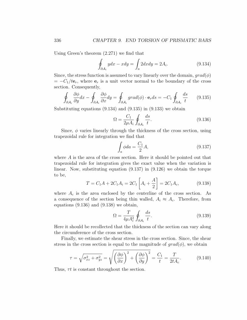
336 CHAPTER 9. END TORSION OF PRISMATIC BARS
Using Green’s theorem (2.271) we find that∮∂Ai
ydx− xdy =
∫a
2dxdy = 2Ai. (9.134)
Since, the stress function is assumed to vary linearly over the domain, grad(φ)= −C1/ter, where er is a unit vector normal to the boundary of the crosssection. Consequently,∮
∂Ai
∂φ
∂ydx−
∮∂Ai
∂φ
∂xdy =
∮∂Ai
grad(φ) · erds = −C1
∮∂Ai
ds
t(9.135)
Substituting equations (9.134) and (9.135) in (9.133) we obtain
Ω =C1
2µAi
∮∂Ai
ds
t. (9.136)
Since, φ varies linearly through the thickness of the cross section, usingtrapezoidal rule for integration we find that∫
a
φda =C1
2A, (9.137)
where A is the area of the cross section. Here it should be pointed out thattrapezoidal rule for integration gives the exact value when the variation islinear. Now, substituting equation (9.137) in (9.126) we obtain the torqueto be,
T = C1A+ 2C1Ai = 2C1
[Ai +
A
2
]= 2C1Ac, (9.138)
where Ac is the area enclosed by the centerline of the cross section. Asa consequence of the section being thin walled, Ai ≈ Ac. Therefore, fromequations (9.136) and (9.138) we obtain,
Ω =T
4µA2c
∮∂Ai
ds
t. (9.139)
Here it should be recollected that the thickness of the section can vary alongthe circumference of the cross section.
Finally, we estimate the shear stress in the cross section. Since, the shearstress in the cross section is equal to the magnitude of grad(φ), we obtain
τ =√σ2xz + σ2
yz =
√(∂φ
∂x
)2
+
(∂φ
∂y
)2
=C1
t=
T
2tAc. (9.140)
Thus, τt is constant throughout the section.
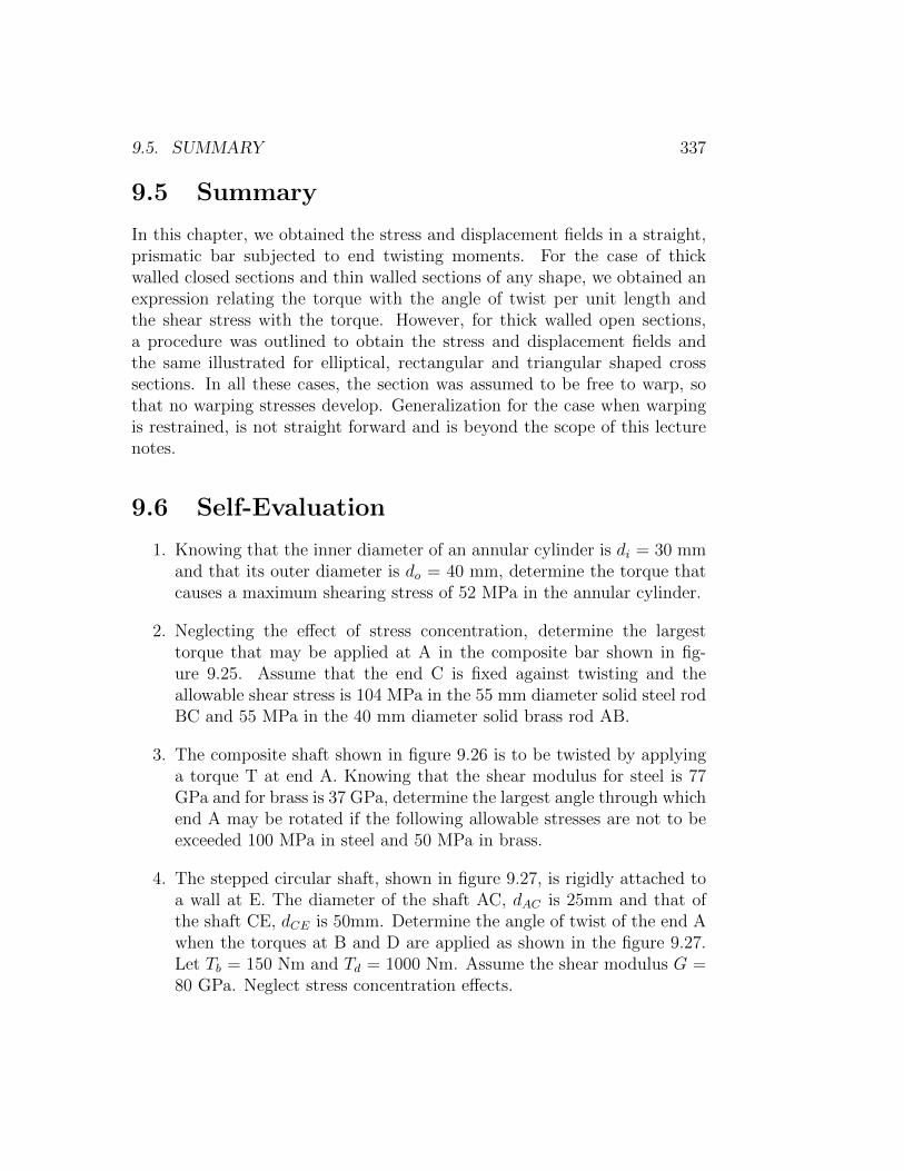
9.5. SUMMARY 337
9.5 Summary
In this chapter, we obtained the stress and displacement fields in a straight,prismatic bar subjected to end twisting moments. For the case of thickwalled closed sections and thin walled sections of any shape, we obtained anexpression relating the torque with the angle of twist per unit length andthe shear stress with the torque. However, for thick walled open sections,a procedure was outlined to obtain the stress and displacement fields andthe same illustrated for elliptical, rectangular and triangular shaped crosssections. In all these cases, the section was assumed to be free to warp, sothat no warping stresses develop. Generalization for the case when warpingis restrained, is not straight forward and is beyond the scope of this lecturenotes.
9.6 Self-Evaluation
1. Knowing that the inner diameter of an annular cylinder is di = 30 mmand that its outer diameter is do = 40 mm, determine the torque thatcauses a maximum shearing stress of 52 MPa in the annular cylinder.
2. Neglecting the effect of stress concentration, determine the largesttorque that may be applied at A in the composite bar shown in fig-ure 9.25. Assume that the end C is fixed against twisting and theallowable shear stress is 104 MPa in the 55 mm diameter solid steel rodBC and 55 MPa in the 40 mm diameter solid brass rod AB.
3. The composite shaft shown in figure 9.26 is to be twisted by applyinga torque T at end A. Knowing that the shear modulus for steel is 77GPa and for brass is 37 GPa, determine the largest angle through whichend A may be rotated if the following allowable stresses are not to beexceeded 100 MPa in steel and 50 MPa in brass.
4. The stepped circular shaft, shown in figure 9.27, is rigidly attached toa wall at E. The diameter of the shaft AC, dAC is 25mm and that ofthe shaft CE, dCE is 50mm. Determine the angle of twist of the end Awhen the torques at B and D are applied as shown in the figure 9.27.Let Tb = 150 Nm and Td = 1000 Nm. Assume the shear modulus G =80 GPa. Neglect stress concentration effects.
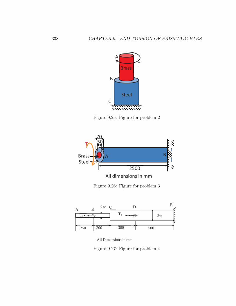
338 CHAPTER 9. END TORSION OF PRISMATIC BARS
A
B
C
Brass
Steel
T
Figure 9.25: Figure for problem 2
2500 All dimensions in mm
70 70750
A B Steel Brass
T
Figure 9.26: Figure for problem 3
All Dimensions in mm
A
500
E
300 200 250
D C B Td Tb dCE
dAC
Figure 9.27: Figure for problem 4

9.6. SELF-EVALUATION 339
All Dimensions in mm
A
500
E
300 200 250
D C B
Td Tb dCE
dAC
Figure 9.28: Figure for problem 5
5. (a) Determine the reactions for the circular stepped shafts shown infigure 9.28. Let the diameter of the shaft AC, dAC be 25mm and thatof the shaft CE, dCE be 50mm and the torques, Tb = 400 Nm and Td= 2000 Nm. (b) Plot the angle of twist diagram for the shaft along itslength. The material parameters for the material with which this shaftis made are: Young’s modulus, E = 120 GPa and Poisson’s ratio, ν =1/3. Neglect stress concentration effects.
6. Same torque is applied to two hollow shafts of same length 0.5 m andmade of same material but having cross sections in the shape of T andC, as shown in figure 9.29. Neglecting the effect of stress concentration,compare the maximum shearing stress that occurs in these sections andthe angle of twist of the shaft. Assume, tw = t = 6 mm, tf = 12 mm,b = 25 mm, h = 30 mm. Recognizing that the area of both the crosssections is same, comment on which section is economical.
7. Verify that the admissibility of the following Prandtl stress function fora circular shaft with a keyway, as shown in figure 9.30,
φ = K(b2 − r2)
(1− 2a cos(θ)
r
),
where K is a constant. If the stress function is admissible,
(a) Find the constant K
(b) Compute the Cartesian components of the shear stress, σxz andσyz
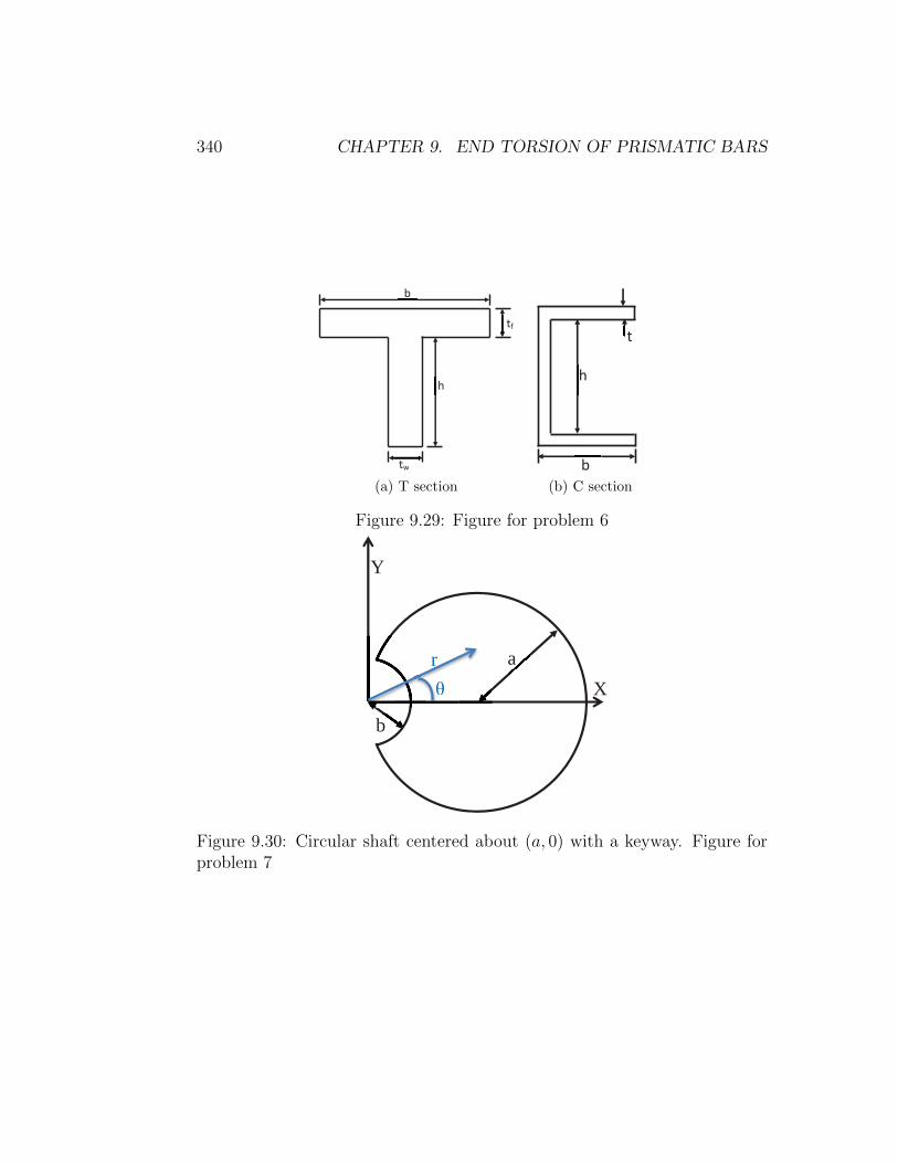
340 CHAPTER 9. END TORSION OF PRISMATIC BARS
tw
tf
b
h
(a) T section
h
b
t
(b) C section
Figure 9.29: Figure for problem 6
a X
Y
b
r θ rθθ
Figure 9.30: Circular shaft centered about (a, 0) with a keyway. Figure forproblem 7
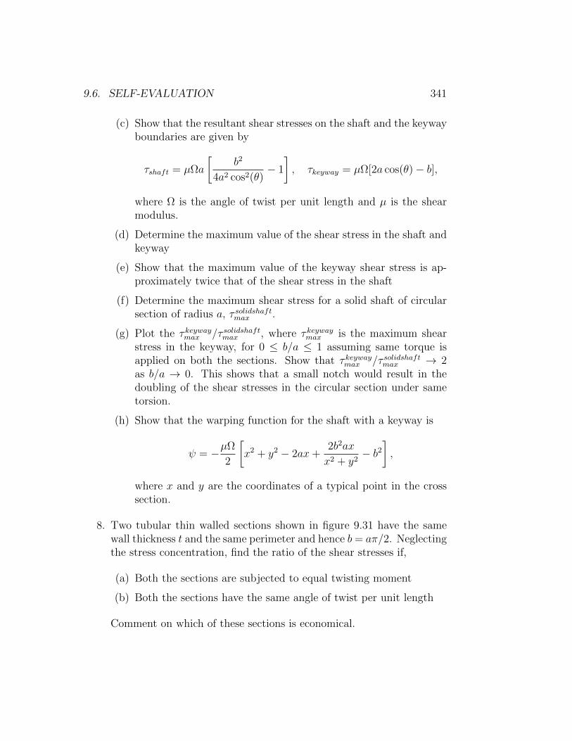
9.6. SELF-EVALUATION 341
(c) Show that the resultant shear stresses on the shaft and the keywayboundaries are given by
τshaft = µΩa
[b2
4a2 cos2(θ)− 1
], τkeyway = µΩ[2a cos(θ)− b],
where Ω is the angle of twist per unit length and µ is the shearmodulus.
(d) Determine the maximum value of the shear stress in the shaft andkeyway
(e) Show that the maximum value of the keyway shear stress is ap-proximately twice that of the shear stress in the shaft
(f) Determine the maximum shear stress for a solid shaft of circularsection of radius a, τ solidshaftmax .
(g) Plot the τ keywaymax /τ solidshaftmax , where τ keywaymax is the maximum shearstress in the keyway, for 0 ≤ b/a ≤ 1 assuming same torque isapplied on both the sections. Show that τ keywaymax /τ solidshaftmax → 2as b/a → 0. This shows that a small notch would result in thedoubling of the shear stresses in the circular section under sametorsion.
(h) Show that the warping function for the shaft with a keyway is
ψ = −µΩ
2
[x2 + y2 − 2ax+
2b2ax
x2 + y2− b2
],
where x and y are the coordinates of a typical point in the crosssection.
8. Two tubular thin walled sections shown in figure 9.31 have the samewall thickness t and the same perimeter and hence b = aπ/2. Neglectingthe stress concentration, find the ratio of the shear stresses if,
(a) Both the sections are subjected to equal twisting moment
(b) Both the sections have the same angle of twist per unit length
Comment on which of these sections is economical.
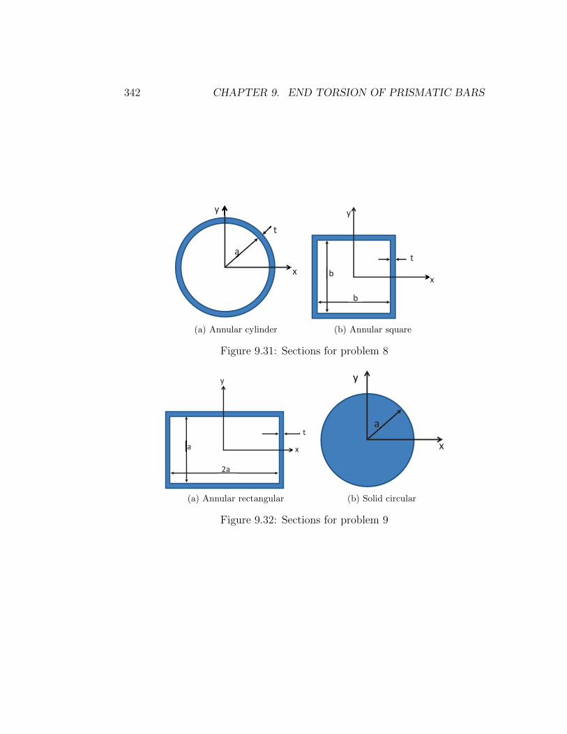
342 CHAPTER 9. END TORSION OF PRISMATIC BARS
a
t
x
y
(a) Annular cylinder
t
b
b
x
y
(b) Annular square
Figure 9.31: Sections for problem 8
t
a
2a
x
y
(a) Annular rectangular
y
a
y
x
(b) Solid circular
Figure 9.32: Sections for problem 9

9.6. SELF-EVALUATION 343
9. Two sections, a solid circular section and a hollow rectangular tubeas shown in figure 9.32 are subjected to the same torque, T . If thetwo tubes are of same length, L and made of the same material anddiffer only in the shape of the cross section, find the thickness of therectangular section so that (a) the maximum shear stresses is same inboth the sections (b) angle of twist per unit length is same for thesetwo sections. Comment on which of these sections is economical.
10. During the early development of the torsion formulation, Navier as-sumed that there is no warping displacement for any cross section.Show that although such an assumed displacement field will satisfy allthe required governing differential equations, it would not satisfy theboundary conditions and hence this is not an acceptable solution.

344 CHAPTER 9. END TORSION OF PRISMATIC BARS

Chapter 10
Bending of Curved Beams
10.1 Overview
Till now, we have been studying members that are initially straight. In thischapter, we shall study the bending of beams which are initially curved. Wedo this by restricting ourselves to the case where the bending takes place inthe plane of curvature. This happens when the cross section of the beam issymmetrical about the plane of its curvature and the bending moment acts inthis plane. As we did for straight beams, we first obtain the solution assumingsections that are initially plane remain plane after bending. The resultingrelation between the stress, moment and the deflection is called as Winkler-Bach formula. Then, using the two dimensional elasticity formulation, weobtain the stress and displacement field without assuming plane sectionsremain plane albeit for a particular cross section of a curved beam subjectedto a pure bending moment or end load. We conclude by comparing boththe solutions to find that they are in excellent agreement when the beam isshallow.
Before proceeding further, we would like to clarify what we mean by acurved beam. Beam whose axis is not straight and is curved in the elevationis said to be a curved beam. If the applied loads are along the y direction andthe span of the beam is along the x direction, the axis of the beam shouldhave a curvature in the xy plane. On the hand, if the member is curvedon the xz plane with the loading still along the y direction, then it is not acurved beam, as this loading will cause a bending as well as twisting of thesection. Thus, a curved beam does not have a curvature in the plan. Arches
345
346 CHAPTER 10. BENDING OF CURVED BEAMS
A F
A’
M M
C S
G C N
y
r
B B’
ΔΦ
δΔΦ
(a) Elevation view: projection in the xyplane.
y
x
N -y
N
C
(b) Isotropic view.
Figure 10.1: Schematic of bending of a curved beam
are examples of curved beams.
10.2 Winkler-Bach formula for curved beams
As mentioned before, in this section we obtain the stress field assuming,sections that are plane before bending remain plane after bending. Conse-quently, a transverse section rotates about an axis called the neutral axis asshown in figure 10.1. Let us examine an infinitesimal portion of a curvedbeam enclosing an angle ∆φ. Due to an applied pure bending moment M ,the section AB rotates through an angle δ(∆φ) about the neutral axis andoccupy the position A′B′. SN denotes the surface on which the stress iszero and is called the neutral surface. Since, the stress is zero in this neutralsurface, the length of the material fibers on this plane and oriented along theaxis of the beam would not have changed. However, fibers above the neutralsurface and oriented along the axis of the beam would be in compression andthose below the neutral surface and oriented along the axis of the beam wouldbe in tension. Hence, for a fiber at a distance y from the neutral surface, itslength before the deformation would be (rn−y)∆φ, where rn is the radius ofcurvature of the neutral surface. The change in length of the same fiber after

10.2. WINKLER-BACH FORMULA FOR CURVED BEAMS 347
deformation due to the applied bending moment, M would be −y(δ(∆φ)).Note that the negative sign is to indicate that the length reduces when y ispositive for the direction of the moment indicated in the figure 10.1. Thus,the linearized strain is given by,
ε = − y(δ(∆φ))
(rn − y)(∆φ). (10.1)
It is assumed that the lateral dimensions of the beam are unaltered dueto bending, i.e. the Poisson’s effect is ignored. Hence, the quantity y re-mains unaltered due to the deformation. Now, to estimate the quantityδ(∆φ)/(∆φ), we observe from figure 10.1a that
SN = r(∆φ+ δ(∆φ)), (10.2)
where r is the radius of curvature of the neutral axis after bending. However,by virtue of it being neutral surface, its length is unaltered and therefore
SN = rn∆φ. (10.3)
Equating equations (10.2) and (10.3) and simplifying we obtain
δ(∆φ)
∆φ=rnr− 1. (10.4)
Substituting equation (10.4) in (10.1) we obtain,
ε = − y
rn − y
[rnr− 1]. (10.5)
Having obtained the strain, the expression for the stress becomes
σ = −E y
rn − y
[rnr− 1], (10.6)
where E is the Young’s modulus and we have appealed to one dimensionalHooke’s law to relate the strain and the stress.
Since, we assume that the section is subjected to pure bending momentand in particular no axial load, we require that∫
a
σda = −∫a
Ey
rn − y
[rnr− 1]da = 0, (10.7)

348 CHAPTER 10. BENDING OF CURVED BEAMS
where we have used (10.6). Since, rn and r are constants for a given sectionand r 6= rn, when the beam deforms, for equation (10.7) to hold,∫
a
Ey
rn − yda = 0. (10.8)
We have to find rn such that (10.8) holds. Observing that y/(rn − y) =rn/(rn − y)− 1, equation (10.8) can be simplified as
rn
∫a
E
rn − yda−
∫a
Eda = 0. (10.9)
If the section is homogeneous, Young’s modulus is constant over the sectionand therefore the above equation can be written as,
rn =A∫
ada
rn−y(10.10)
Assuming the bending moment at the section being studied is M , asshown in section 8.1, equation (8.9),
M = −∫a
yσda, (10.11)
where we have assumed that the origin of the coordinate system is located atthe neutral axis of the section; consistent with the assumption made while ob-taining the expression for the strain. Substituting equation (10.7) in (10.11)and rewriting we obtain,
M =[rnr− 1] ∫
a
Ey2
rn − yda =
[rnr− 1] ∫
a
E
[rn
y
rn − y− y]da
=[rnr− 1] [rn
∫a
Ey
rn − yda−
∫a
Eyda
]. (10.12)
It follows from (10.8) that the first integral in the above equation is zero.Thus, equation (10.12) simplifies to[rn
r− 1]
= − M∫aEyda
. (10.13)

10.2. WINKLER-BACH FORMULA FOR CURVED BEAMS 349
Then, combining equation (10.6) and (10.13) we obtain
−[rnr− 1]
=M∫
aEyda
=σ
E
rn − yy
, (10.14)
where rn is obtained by solving (10.9). If the section is homogeneous that isE is constant over the section equation (10.14) simplifies to,
− E[rnr− 1]
=M∫ayda
= σrn − yy
, (10.15)
where rn is obtained by solving (10.10). Note that in these equations y ismeasured from the neutral axis of the section and the bending moment thatincreases the curvature (decreases the radius of curvature) is assumed to bepositive.
Thus, given the moment in the section, using equation (10.14) or (10.15),we can estimate the stress (σ) distribution in the section and/or the deformedcurvature (r) of the beam. These equations are called Winkler-Bach formulafor curved beams.
Next, we illustrate a technique to find the radius of curvature of theneutral surface, rn for a homogeneous rectangular section. Consider a rect-angular section shown in figure 10.2 where ρo denotes the radius of curvatureof the centroid of the cross section, ri the radius of curvature of the topmostfiber of the cross section and ro the radius of curvature of the bottommostfiber of the cross section. Let u = rn − y. Now, u is the location of a fiberfrom the center of curvature of the section,as indicated in the figure 10.2.Hence, ∫
a
da
rn − y=
∫ ro
ri
bdu
u= b ln
(rori
). (10.16)
Consequently, the value of rn, the radius of curvature of the neutral axis fora rectangular section as determined from (10.10) is
rn =bh
b ln(rori
) =h
ln(rori
) . (10.17)
Having obtained rn, we would like to obtain the stress distribution in acurved beam with rectangular section subjected to a moment M . It followsfrom equation (10.15) that
σ =y
rn − yM∫ayda
. (10.18)
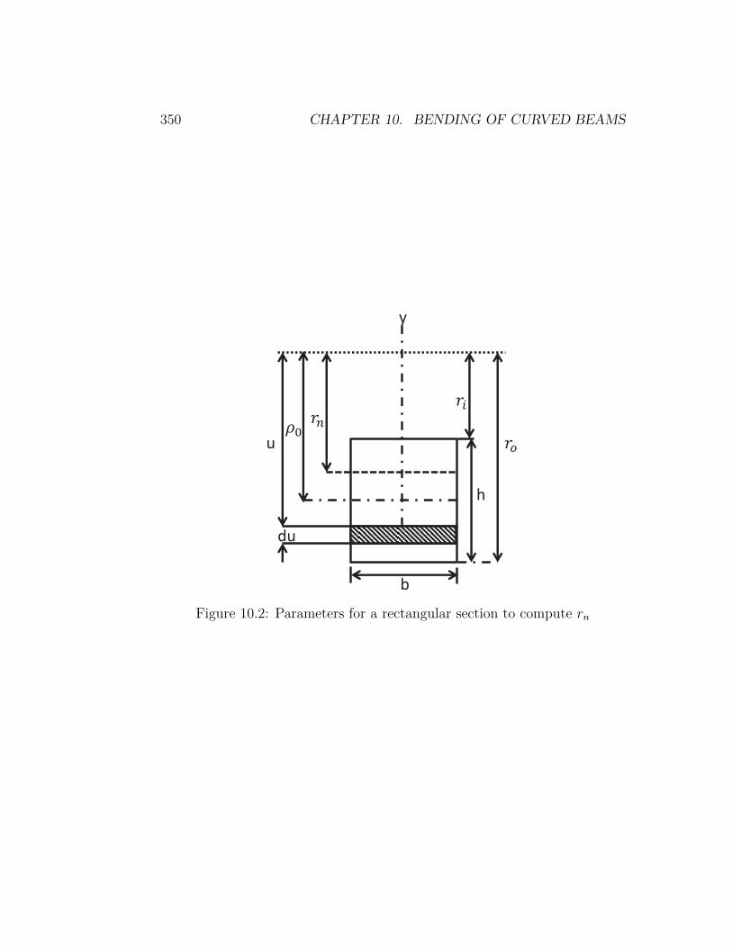
350 CHAPTER 10. BENDING OF CURVED BEAMS
y
h
b
u
du
Figure 10.2: Parameters for a rectangular section to compute rn
10.3. 2D ELASTICITY SOLUTION FOR CURVED BEAMS 351
Now we need to compute∫ayda with y measured from the neutral axis.
Towards this,∫a
yda =
∫ ro
ri
(rn − u)bdu = b
[rn(ro − ri)−
1
2(r2o − r2
i )
]= bh [rn − ρo] ,
(10.19)where we have used the fact that ro−ri = h and ρo = (ro+ri)/2. Substitutingequation (10.19) in (10.18), we obtain
σ =My
bh(rn − y)[rn − (ri + ro)/2], (10.20)
where rn − ro ≤ y ≤ rn − ri. We compare the qualitative features of thissolution after obtaining the elasticity solution.
10.3 2D Elasticity solution for curved beams
In this section, we obtain the two dimensional elasticity solution for thecurved beam subjected to pure bending and end loading. The cross sectionof the beam is assumed to be rectangular of width 2b and depth h. Asthe beam is curved, we use cylindrical polar coordinates to formulate andstudy this problem. The curved beam is assumed to be the annular regionbetween two coaxial radially cut cylinders of radius ri and ri + h, i.e, B =(r, θ, z)|ri ≤ r ≤ ro, α1 ≤ θ ≤ α2,−b ≤ z ≤ b, where ri, ro, α1, α2 and bare constants. Note that here ro = ri + h
10.3.1 Pure bending
The first example that we study, is that of pure bending of a curved beam.Here the curved beam is assumed to be subjected to end moments as shownin figure 10.3. The traction boundary conditions for this problem are
(a) The surfaces defined by r = ri and r = ro are traction free.
(b) The surfaces defined by θ = ±α though is subjected to a moment, Malong the z direction, has no net force.
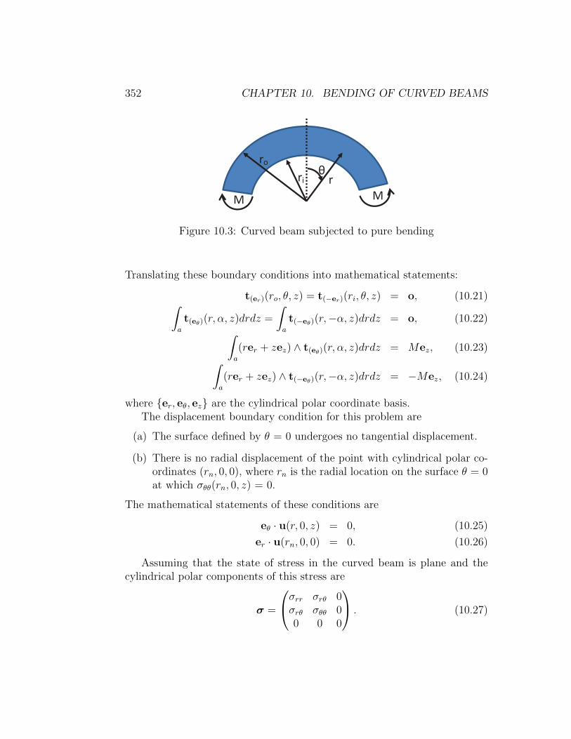
352 CHAPTER 10. BENDING OF CURVED BEAMS
M M
ro ri r
θ
Figure 10.3: Curved beam subjected to pure bending
Translating these boundary conditions into mathematical statements:
t(er)(ro, θ, z) = t(−er)(ri, θ, z) = o, (10.21)∫a
t(eθ)(r, α, z)drdz =
∫a
t(−eθ)(r,−α, z)drdz = o, (10.22)∫a
(rer + zez) ∧ t(eθ)(r, α, z)drdz = Mez, (10.23)∫a
(rer + zez) ∧ t(−eθ)(r,−α, z)drdz = −Mez, (10.24)
where er, eθ, ez are the cylindrical polar coordinate basis.The displacement boundary condition for this problem are
(a) The surface defined by θ = 0 undergoes no tangential displacement.
(b) There is no radial displacement of the point with cylindrical polar co-ordinates (rn, 0, 0), where rn is the radial location on the surface θ = 0at which σθθ(rn, 0, z) = 0.
The mathematical statements of these conditions are
eθ · u(r, 0, z) = 0, (10.25)
er · u(rn, 0, 0) = 0. (10.26)
Assuming that the state of stress in the curved beam is plane and thecylindrical polar components of this stress are
σ =
σrr σrθ 0σrθ σθθ 00 0 0
. (10.27)

10.3. 2D ELASTICITY SOLUTION FOR CURVED BEAMS 353
Substituting the above stress (10.27) in the traction boundary conditions(10.21) through (10.24) we obtain,
σrr(ri, θ, z) = σrr(ro, θ, z) = 0, (10.28)
σrθ(ri, θ, z) = σrθ(ro, θ, z) = 0, (10.29)∫a
σrθ(r,±α, z)drdz = 0, (10.30)∫a
σθθ(r,±α, z)drdz = 0, (10.31)∫a
zσrθ(r,±α, z)drdz = 0, (10.32)∫a
rσθθ(r,±α, z)drdz = M. (10.33)
Now, we have to find Airy’s stress function, φ that would satisfy theboundary conditions (10.28) through (10.33) and the bi-harmonic equation.In this problem we expect the stresses to be such that σ(r, θ, z) = σ(r,−θ, z),for any θ, i.e. the stress is an even function of θ. Imposing this restrictionthat the stress be an even function of θ, on the general periodic solution tothe bi-harmonic solution (7.57), results in requiring that the Airy’s stressfunction be independent of θ. Thus, Airy’s stress function is,
φ = a01 + a02 ln(r) + a03r2 + a04r
2 ln(r), (10.34)
where the constants a0i’s are to be found from the boundary conditions. Thestress field corresponding to this Airy’s stress function, (10.34) found using(7.53) is
σrr = 2a04 ln(r) +a02
r2+ a04 + 2a03, (10.35)
σθθ = 2a04 ln(r)− a02
r2+ 3a04 + 2a03, (10.36)
σrθ = 0. (10.37)
It can be immediately seen that by virtue of σrθ = 0, boundary conditions(10.29), (10.30) and (10.32) are trivially satisfied. The boundary condition(10.28) requires that
2a04 ln(ri) +a02
r2i
+ a04 + 2a03 = 0, (10.38)
2a04 ln(ro) +a02
r2o
+ a04 + 2a03 = 0. (10.39)
354 CHAPTER 10. BENDING OF CURVED BEAMS
The boundary condition (10.31) requires that
ro
[2a04 ln(ro) +
a02
r2o
+ a04 + 2a03
]− ri
[2a04 ln(ri) +
a02
r2i
+ a04 + 2a03
]= 0.
(10.40)By virtue of the terms in the square brackets being same as those in equations(10.39) and (10.38), equation (10.40) holds if (10.38) and (10.39) are satisfied.The only remaining boundary condition (10.33) when evaluated mandatesthat
a04[r2o ln(ro)− r2
i ln(ri)]− a02 ln
(rori
)+ (a04 + a03)(r2
o − r2i ) =
M
2b. (10.41)
Solving equations (10.38), (10.39) and (10.41) for the unknown constantsa0i’s, we obtain
a02 =M
N4r2
i r2o ln
(rori
), (10.42)
a03 = −MN
[r2o − r2
i + 2(r2o ln(ro)− r2
i ln(ri))], (10.43)
a04 =M
N2[r2
o − r2i ], (10.44)
where
N = 2b
(r2o − r2
i )2 − 4r2
i r2o
[ln
(rori
)]2. (10.45)
Substituting these constants from equation (10.42) through (10.44) in theexpression for the stresses (10.35) through (10.37) the stress field becomesknown.
In figure 10.4 we compare the bending stress (σθθ) obtained using theWinkler-Bach formula with that obtained using the two dimensional elastic-ity approach. We find that both these approaches though predict differentexpressions for the stress, evaluate to the same values as seen from figure10.4b. However, differences between these approaches increases as ri/h valuetends to zero as seen from figure 10.4a.
In figure 10.5 we study when critical curvature of the beam above whichthe stresses in the beam are not influenced much by the curvature. It seemsthat if the curvature of the innermost fiber exceeds 5 times the depth of the

10.3. 2D ELASTICITY SOLUTION FOR CURVED BEAMS 355
−30 −20 −10 0 100
0.2
0.4
0.6
0.8
1
σ bh2/M
(ro−
r)/h
ri/h = 0.05−ELS
ri/h = 0.05−WB
(a) Beam with large initial curvature
−20 −10 0 100
0.2
0.4
0.6
0.8
1
σ bh2/M
(ro−
r)/h
ri/h = 0.1−ELS
ri/h = 0.1−WB
(b) Beam with moderate initial curva-ture
Figure 10.4: Comparison of the Winkler-Bach formula for the stress in thecurved beams with the two dimensional elasticity solution for beams withdifferent initial curvatures
−10 −5 0 5 100
0.2
0.4
0.6
0.8
1
σ bh2/M
(ro−
r)/h
ri/h = 4−ELS
ri/h = 4−WB
(a) Beam with small initial curvature
−10 −5 0 5 100
0.2
0.4
0.6
0.8
1
σ bh2/M
(ro−
r)/h
ri/h = 12−ELS
ri/h = 12−WB
(b) Beam with negligible initial curva-ture
Figure 10.5: Study on the influence of initial curvature of the beam on thebending stresses developed due to a given moment
356 CHAPTER 10. BENDING OF CURVED BEAMS
beam with rectangular cross section, one can consider the beam as straightfor practical purposes.
Having obtained the stress field that satisfies the compatibility conditions,a smooth displacement field corresponding to this stress field can be deter-mined by following the standard approach of estimating the strains for thisstress field from the two dimensional constitutive relation and then integrat-ing the resulting strains for the displacements using the strain displacementrelation. On performing these calculations, we find that the cylindrical polarcomponents of the displacement field are given by
ur =1
E
[2(1− ν)(a04r ln(r) + a03r)− (1 + ν)
(a02
r+ a04r
)]+ C1 sin(θ) + C2 cos(θ), (10.46)
uθ =4a04
Erθ + C1 cos(θ)− C2 sin(θ) + C3r, (10.47)
where Ci’s are constants to be determined from the displacement boundaryconditions, ur is the radial component of the displacement and uθ is thetangential component of the displacement.
Substituting equation (10.47) in the displacement boundary condition(10.25) we obtain,
C1 + C3r = 0. (10.48)
For equation (10.48) to hold,
C1 = 0, C3 = 0. (10.49)
In order to satisfy the displacement boundary condition (10.26),
C2 = − 1
E
[2(1− ν)(a04rn ln(rn) + a03rn)− (1 + ν)
(a02
rn+ a04rn
)].
(10.50)
10.3.2 Curved cantilever beam under end load
The next example that we study, is that of end loading of a curved cantileverbeam. Here a cantilever beam is assumed to be subjected to end shear forceas shown in figure 10.6. Thus, the displacement boundary condition for thisproblem is
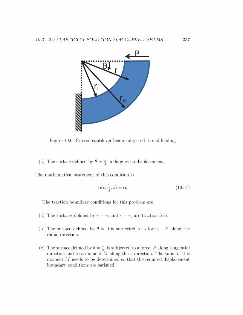
10.3. 2D ELASTICITY SOLUTION FOR CURVED BEAMS 357
θ
ri
ro
r
P
Figure 10.6: Curved cantilever beam subjected to end loading
(a) The surface defined by θ = π2
undergoes no displacement.
The mathematical statement of this condition is
u(r,π
2, z) = o, (10.51)
The traction boundary conditions for this problem are
(a) The surfaces defined by r = ri and r = ro are traction free.
(b) The surface defined by θ = 0 is subjected to a force, −P along theradial direction.
(c) The surface defined by θ = π2, is subjected to a force, P along tangential
direction and to a moment M along the z direction. The value of thismoment M needs to be determined so that the required displacementboundary conditions are satisfied.

358 CHAPTER 10. BENDING OF CURVED BEAMS
Translating these boundary conditions into mathematical statements:
t(er)(ro, θ, z) = t(−er)(ri, θ, z) = o, (10.52)∫a
t(eθ)(r, 0, z)drdz = −Per, (10.53)∫a
t(−eθ)
(r,π
2, z)drdz = Peθ, (10.54)∫
a
(rer + zez) ∧ t(eθ)(r, 0, z)drdz = o, (10.55)∫a
(rer + zez) ∧ t(−eθ)
(r,π
2, z)drdz = −Mez, (10.56)
where er, eθ, ez are the cylindrical polar coordinate basis.
Assuming that the state of stress in the curved beam is plane and thecylindrical polar components of this stress are
σ =
σrr σrθ 0σrθ σθθ 00 0 0
. (10.57)
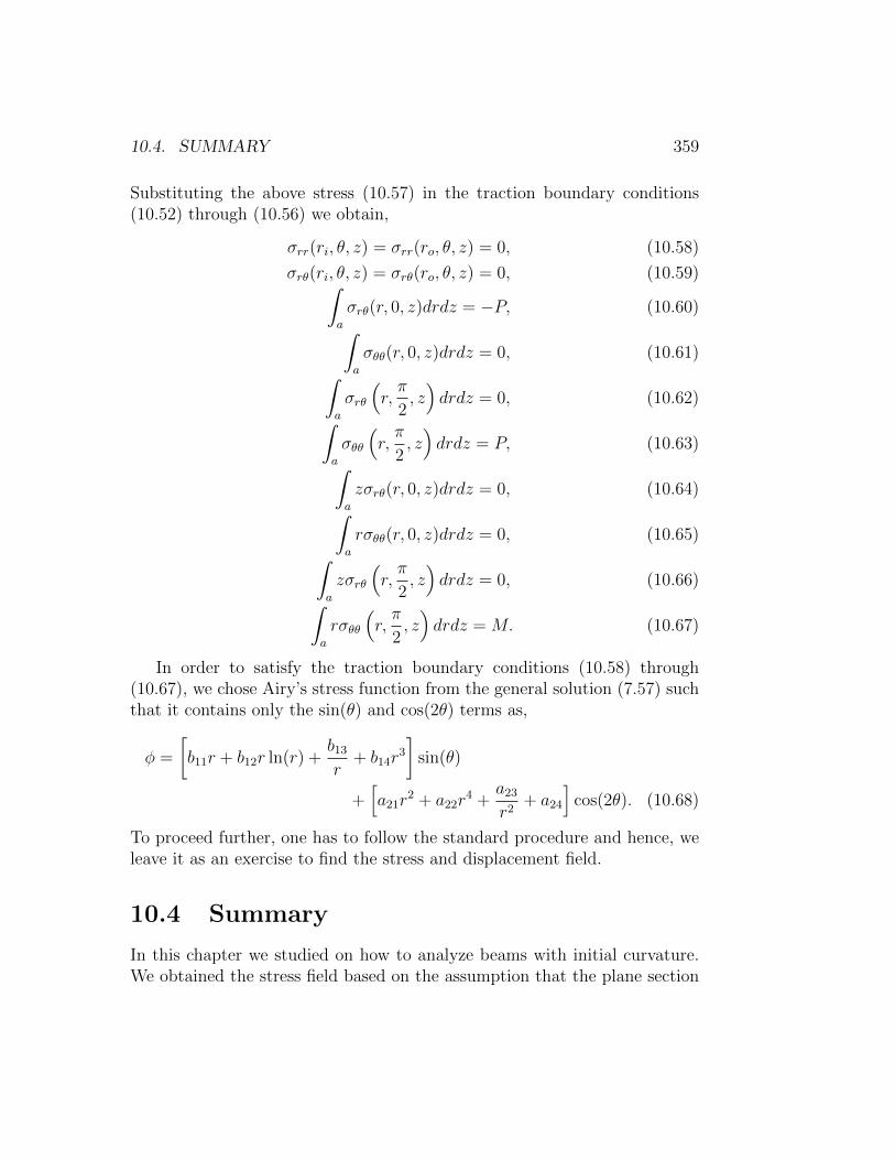
10.4. SUMMARY 359
Substituting the above stress (10.57) in the traction boundary conditions(10.52) through (10.56) we obtain,
σrr(ri, θ, z) = σrr(ro, θ, z) = 0, (10.58)
σrθ(ri, θ, z) = σrθ(ro, θ, z) = 0, (10.59)∫a
σrθ(r, 0, z)drdz = −P, (10.60)∫a
σθθ(r, 0, z)drdz = 0, (10.61)∫a
σrθ
(r,π
2, z)drdz = 0, (10.62)∫
a
σθθ
(r,π
2, z)drdz = P, (10.63)∫
a
zσrθ(r, 0, z)drdz = 0, (10.64)∫a
rσθθ(r, 0, z)drdz = 0, (10.65)∫a
zσrθ
(r,π
2, z)drdz = 0, (10.66)∫
a
rσθθ
(r,π
2, z)drdz = M. (10.67)
In order to satisfy the traction boundary conditions (10.58) through(10.67), we chose Airy’s stress function from the general solution (7.57) suchthat it contains only the sin(θ) and cos(2θ) terms as,
φ =
[b11r + b12r ln(r) +
b13
r+ b14r
3
]sin(θ)
+[a21r
2 + a22r4 +
a23
r2+ a24
]cos(2θ). (10.68)
To proceed further, one has to follow the standard procedure and hence, weleave it as an exercise to find the stress and displacement field.
10.4 Summary
In this chapter we studied on how to analyze beams with initial curvature.We obtained the stress field based on the assumption that the plane section

360 CHAPTER 10. BENDING OF CURVED BEAMS
remain plane after bending. We also obtained two dimensional elasticitysolution which is not based on the assumption that plane sections remainplane. However, we found that both these solutions predict the same valueof stresses for practically used curved beams.
10.5 Self-Evaluation
1. There are two beams - a straight beam and a curved beam - each ofwhich is subjected to a pure bending moment, M. Assuming that boththe beams are homogeneous and has a square cross section with side0.3m and are made of the same material, which is linear elastic andisotropic, compute the ratio of the maximum tensile stresses experi-enced in the straight and curved beams. Also, find the ratio of themaximum compressive stresses experienced in the straight and curvedbeams. Assume, the curved beam forms a part of a circle, with the ini-tial radius of curvature of the center line of the bar, being ρo. Obtainthe value of the ratios as a function of ρo and determine the criticalrhoco below which the stresses would differ by more than 10 percent.
2. A curved beam with a circular center line has the T-section as shownin figure 10.7. This beam is subjected to pure bending in its plane ofsymmetry. Find the tensile and compressive stresses in the extremefibers. Assume, b1 = 100 mm, b2 = 20 mm, the radius of curvature ofthe innermost fiber, r1 = 80 mm, the outermost fiber, r2 = 180 mmand r3 = 100 mm.
3. A curved beam with a circular center line has the circular sections asshown in figure 10.8. Find the stress distribution across this section ifthe curved beam is subjected to a pure bending moment, M . Assumethat the initial curvature of the center line of the beam is ρo.
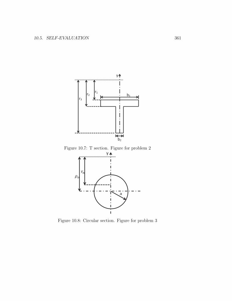
10.5. SELF-EVALUATION 361
r1 r2 r3
y
b1
b2
Figure 10.7: T section. Figure for problem 2
a
y
Figure 10.8: Circular section. Figure for problem 3

362 CHAPTER 10. BENDING OF CURVED BEAMS

Chapter 11
Beam on Elastic Foundation
11.1 Overview
In some applications such as rail tracks, the member subjected to loads issupported on continuous foundations. That is the reactions due to externalloading is distributed along the length of the member. Here we study on howto get the stresses and displacements in these members resting on continuousfoundations. If the dimensions of this member is such that, it is longeralong one of the axis, called the longitudinal axis in comparison with thedimensions along the other directions, it is called as a beam. If we assumethat the reaction force offered by the continuous support is a function of thedisplacement that of the member, the support is called as elastic. A beamresting on an elastic support is said to be beam on elastic foundation.
In this chapter, we first formulate this problem of beam on an elasticfoundation for a general loading condition. Then, we study the problemof a concentrated load at the mid point of a beam that is infinitely long.Appealing to the principle of superposition we obtain the solution to theproblem of a concentrated moment at mid span and uniformly distributedload of length L, centered about the midpoint of the beam.
11.2 General formulation
In this section, we formulate the boundary value problem of beam on anelastic foundation. A beam having some cross section, resting on an elasticsupport is shown in figure 11.1. We assume that the reaction offered by
363
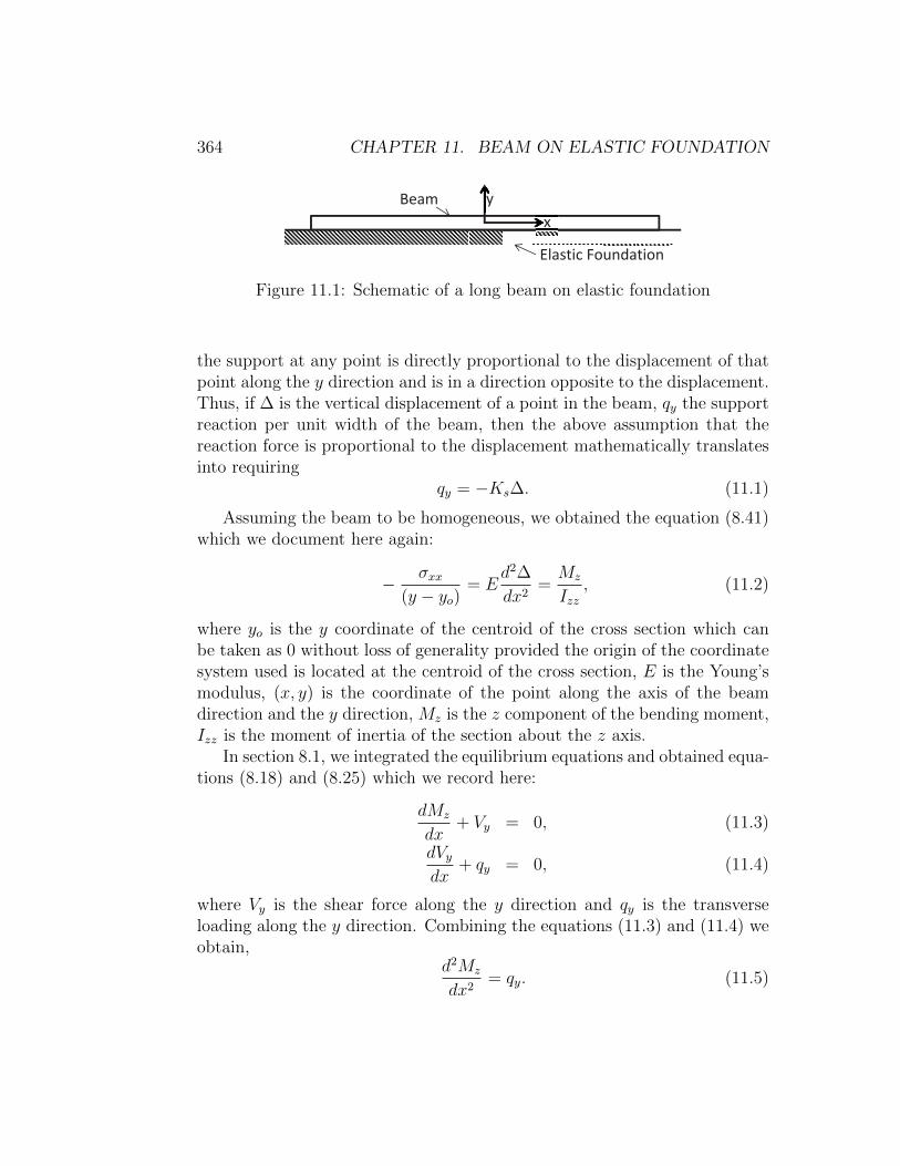
364 CHAPTER 11. BEAM ON ELASTIC FOUNDATION
y x
Beam
Elastic Foundation
Figure 11.1: Schematic of a long beam on elastic foundation
the support at any point is directly proportional to the displacement of thatpoint along the y direction and is in a direction opposite to the displacement.Thus, if ∆ is the vertical displacement of a point in the beam, qy the supportreaction per unit width of the beam, then the above assumption that thereaction force is proportional to the displacement mathematically translatesinto requiring
qy = −Ks∆. (11.1)
Assuming the beam to be homogeneous, we obtained the equation (8.41)which we document here again:
− σxx(y − yo)
= Ed2∆
dx2=Mz
Izz, (11.2)
where yo is the y coordinate of the centroid of the cross section which canbe taken as 0 without loss of generality provided the origin of the coordinatesystem used is located at the centroid of the cross section, E is the Young’smodulus, (x, y) is the coordinate of the point along the axis of the beamdirection and the y direction, Mz is the z component of the bending moment,Izz is the moment of inertia of the section about the z axis.
In section 8.1, we integrated the equilibrium equations and obtained equa-tions (8.18) and (8.25) which we record here:
dMz
dx+ Vy = 0, (11.3)
dVydx
+ qy = 0, (11.4)
where Vy is the shear force along the y direction and qy is the transverseloading along the y direction. Combining the equations (11.3) and (11.4) weobtain,
d2Mz
dx2= qy. (11.5)

11.3. EXAMPLE 1: POINT LOAD 365
Substituting equation (11.2) in equation (11.5), we obtain
d2
dx2
(EIzz
d2∆
dx2
)= qy. (11.6)
Assuming the beam to be homogeneous and prismatic, so that EIzz is con-stant through the length of the beam, and substituting equation (11.1) inequation (11.6), we obtain
EIzzd4∆
dx4= −Ks∆. (11.7)
Defining,
β2 =
√Ks
4EIzz, (11.8)
equation (11.7) can be written as
d4∆
dx4+ 4β4∆ = 0. (11.9)
The differential equation (11.9) has a general solution:
∆ = exp(−βx)[C1 sin(βx) + C2 cos(βx)] + exp(βx)[C3 sin(βx) + C4 cos(βx)],(11.10)
where Ci’s are constant to be determined from the boundary conditions.Having found the deflection, the stress is estimated from (11.2) as
σxx = −E(y − yo)d2∆
dx2
= −2yEβ2 exp(−βx)[C2 sin(βx)− C1 cos(βx)]
+ exp(βx)[C3 cos(βx)− C4 sin(βx)] , (11.11)
where we have assumed that the origin is located at the centroid of the crosssection and hence have set yo = 0.
11.3 Example 1: Point load
The first boundary value problem that we study for the beam on elasticfoundation is when it is subjected to a point load at its mid span as shown
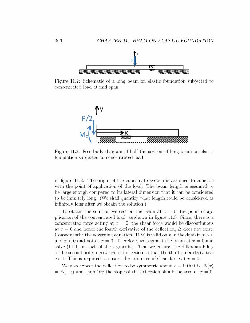
366 CHAPTER 11. BEAM ON ELASTIC FOUNDATION
y
x P
Figure 11.2: Schematic of a long beam on elastic foundation subjected toconcentrated load at mid span
y
x
P/2
Mo
Figure 11.3: Free body diagram of half the section of long beam on elasticfoundation subjected to concentrated load
in figure 11.2. The origin of the coordinate system is assumed to coincidewith the point of application of the load. The beam length is assumed tobe large enough compared to its lateral dimension that it can be consideredto be infinitely long. (We shall quantify what length could be considered asinfinitely long after we obtain the solution.)
To obtain the solution we section the beam at x = 0, the point of ap-plication of the concentrated load, as shown in figure 11.3. Since, there is aconcentrated force acting at x = 0, the shear force would be discontinuousat x = 0 and hence the fourth derivative of the deflection, ∆ does not exist.Consequently, the governing equation (11.9) is valid only in the domain x > 0and x < 0 and not at x = 0. Therefore, we segment the beam at x = 0 andsolve (11.9) on each of the segments. Then, we ensure, the differentiabilityof the second order derivative of deflection so that the third order derivativeexist. This is required to ensure the existence of shear force at x = 0.
We also expect the deflection to be symmetric about x = 0 that is, ∆(x)= ∆(−x) and therefore the slope of the deflection should be zero at x = 0,
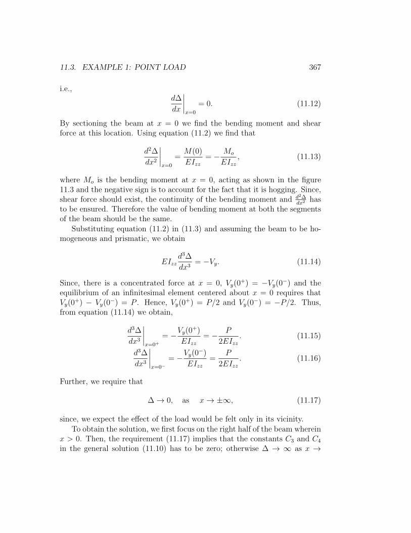
11.3. EXAMPLE 1: POINT LOAD 367
i.e.,d∆
dx
∣∣∣∣x=0
= 0. (11.12)
By sectioning the beam at x = 0 we find the bending moment and shearforce at this location. Using equation (11.2) we find that
d2∆
dx2
∣∣∣∣x=0
=M(0)
EIzz= − Mo
EIzz, (11.13)
where Mo is the bending moment at x = 0, acting as shown in the figure11.3 and the negative sign is to account for the fact that it is hogging. Since,shear force should exist, the continuity of the bending moment and d2∆
dx2has
to be ensured. Therefore the value of bending moment at both the segmentsof the beam should be the same.
Substituting equation (11.2) in (11.3) and assuming the beam to be ho-mogeneous and prismatic, we obtain
EIzzd3∆
dx3= −Vy. (11.14)
Since, there is a concentrated force at x = 0, Vy(0+) = −Vy(0−) and the
equilibrium of an infinitesimal element centered about x = 0 requires thatVy(0
+) − Vy(0−) = P . Hence, Vy(0
+) = P/2 and Vy(0−) = −P/2. Thus,
from equation (11.14) we obtain,
d3∆
dx3
∣∣∣∣x=0+
= −Vy(0+)
EIzz= − P
2EIzz. (11.15)
d3∆
dx3
∣∣∣∣x=0−
= −Vy(0−)
EIzz=
P
2EIzz. (11.16)
Further, we require that
∆→ 0, as x→ ±∞, (11.17)
since, we expect the effect of the load would be felt only in its vicinity.To obtain the solution, we first focus on the right half of the beam wherein
x > 0. Then, the requirement (11.17) implies that the constants C3 and C4
in the general solution (11.10) has to be zero; otherwise ∆ → ∞ as x →
368 CHAPTER 11. BEAM ON ELASTIC FOUNDATION
∞. Next, the condition (11.12) requires that C1 = C2 = C0. Finally, theequation (11.15) tells us that
C0 = − P
8β3EIzz= − Pβ
2Ks
(11.18)
where to obtain the last equality we have made use of (11.8). Thus, in thedomain, x > 0,
∆ = − Pβ2Ks
exp(−βx)[cos(βx) + sin(βx)]. (11.19)
Now, we consider the left half of the beam, i.e., x < 0. The requirement(11.17) implies that the constants C1 and C2 in the general solution (11.10)has to be zero. Next, the condition (11.12) requires that C3 = −C4 = C5.Finally, the equation (11.16) tells us that
C5 = − P
8β3EIzz= − Pβ
2Ks
(11.20)
where to obtain the last equality we have made use of (11.8). Thus, in thedomain, x < 0,
∆ = − Pβ2Ks
exp(βx)[cos(βx)− sin(βx)]. (11.21)
Thus, the distribution of the reaction from the foundation along the axisof the beam given in (11.1) evaluates to:
qy = −Ks∆ =
Pβ2
exp(−βx)[cos(βx) + sin(βx)] x > 0Pβ2
exp(βx)[cos(βx)− sin(βx)] x < 0. (11.22)
The variation of the bending moment along the axis of the beam obtainedfrom (11.2) is:
Mz = EIzzd2∆
dx2=
− P
4βexp(−βx)[cos(βx)− sin(βx)] x ≥ 0
− P4β
exp(βx)[cos(βx) + sin(βx)] x ≤ 0. (11.23)
The shear force variation along the axis of the beam computed using (11.14)is:
Vy = −EIzzd3∆
dx3=
P2
exp(−βx) cos(βx) x ≥ 0−P
2exp(βx) cos(βx) x ≤ 0
. (11.24)
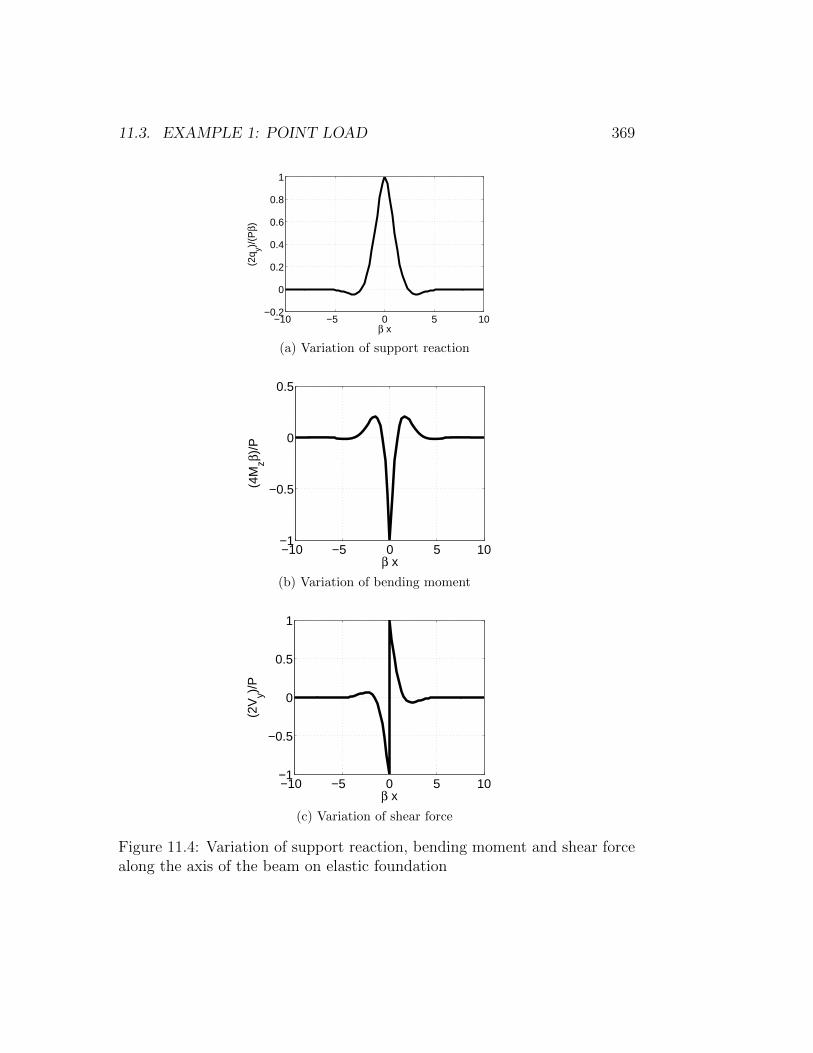
11.3. EXAMPLE 1: POINT LOAD 369
−10 −5 0 5 10−0.2
0
0.2
0.4
0.6
0.8
1
β x
(2q y)/
(Pβ)
(a) Variation of support reaction
−10 −5 0 5 10−1
−0.5
0
0.5
β x
(4M
zβ)/P
(b) Variation of bending moment
−10 −5 0 5 10−1
−0.5
0
0.5
1
β x
(2V
y)/P
(c) Variation of shear force
Figure 11.4: Variation of support reaction, bending moment and shear forcealong the axis of the beam on elastic foundation

370 CHAPTER 11. BEAM ON ELASTIC FOUNDATION
y
x
P P
L/2 2 L/2
Figure 11.5: Schematic of a long beam on elastic foundation subjected toconcentrated moment at mid span
In figure 11.4 we plot the variation of the support reaction, bending mo-ment and shear force along the axis of the beam. It can be seen from thefigure that though the beam is assumed to be infinitely long the reactionforce, bending moment and shear forces all tend to zero for βx > 5. Hence,a beam may be considered as long if its length is greater than, 5/β. It canalso be seen from the figure that the maximum deflection, support reaction,bending moment and shear occurs at z = 0 and these values are,
∆max = − Pβ2Ks
, qmaxy =Pβ
2, Mmax
z = − P4β, V max
y =P
2. (11.25)
It can be seen from figure 11.4a that the support reaction changes sign.The support reaction changes sign at a point when qy = 0, i.e., sin(βx) =− cos(βx) or at x = 3π/(4β). Since, the support reaction is proportional tothe deflection, ∆, this change in sign of the support reaction also tells usthat the beam will uplift at x = ±3π/(4β). Hence, the beams have to beadequately clamped to the foundation to prevent it from uplifting.
11.4 Example 2: Concentrated moment
The concentrated moment, Mo, is considered to be equivalent to the actionof two concentrated forces, P , equal in magnitude but opposite in directionand separated by a distance L as shown in the figure 11.5. Thus,
P =Mo
L. (11.26)
We obtain the solution to this loading case by superposing the displace-ment field obtained in the above example for a single point load. Thus, it

11.4. EXAMPLE 2: CONCENTRATED MOMENT 371
follows from equations (11.17) and (11.19) that the displacement due to thedownward acting force at a distance, L/2 from the origin is,
∆L/2 =
− Pβ
2Ksexp(−β(x− L/2))[cos(β(x− L/2))
+ sin(β(x− L/2))] x ≥ L/2
− Pβ2Ks
exp(β(x− L/2))[cos(β(x− L/2))
− sin(β(x− L/2))] x ≤ L/2
. (11.27)
Similarly, the displacement due to the upward acting force at a distance,−L/2 from the origin is
∆−L/2 =
Pβ2Ks
exp(−β(x+ L/2))[cos(β(x+ L/2))
+ sin(β(x+ L/2))] x ≥ −L/2Pβ2Ks
exp(β(x+ L/2))[cos(β(x+ L/2))
− sin(β(x+ L/2))] x ≤ −L/2
. (11.28)
Since, the displacement is small and the material obeys Hooke’s law, we cansuperpose the solutions as discussed in section 7.5.2. Hence, the displacementunder the action of both the forces, ∆ = ∆L/2 + ∆−L/2 evaluates to,
∆ =
Moβ2KsL
exp(−β(x+ L/2)) [cos(β(x+ L/2))
+ sin(β(x+ L/2))]− exp(−β(x− L/2))[cos(β(x− L/2)) + sin(β(x− L/2))] x ≥ L/2
Moβ2KsL
exp(−β(x+ L/2)) [cos(β(x+ L/2))
+ sin(β(x+ L/2))]− exp(β(x− L/2))[cos(β(x− L/2))− sin(β(x− L/2))] −L/2 ≤ x ≤ L/2
Moβ2KsL
exp(β(x+ L/2)) [cos(β(x+ L/2))
− sin(β(x+ L/2))]− exp(β(x− L/2))[cos(β(x− L/2))− sin(β(x− L/2))] x ≤ −L/2
,
(11.29)where we have used equation (11.26). When L→ 0 and PL→Mo the aboveequation (11.29) evaluates to,
∆ =
−Moβ2
Ksexp(−βx) sin(βx) x ≥ 0
−Moβ2
Ksexp(βx) sin(βx) x ≤ 0
. (11.30)
Having found the displacement, (11.30), the variation of the bendingmoment along the axis of the beam obtained from (11.2) is:
Mz = EIzzd2∆
dx2=
Mo
2exp(−βx) cos(βx) x ≥ 0
−Mo
2exp(βx) cos(βx) x ≤ 0
, (11.31)

372 CHAPTER 11. BEAM ON ELASTIC FOUNDATION
y
x
q L/2 L/2
Figure 11.6: Schematic of a long beam on elastic foundation subjected touniformly distributed load of length L on either side of the mid span
and the shear force variation computed using (11.14) is:
Vy = −EIzzd3∆
dx3=
Moβ
2exp(−βx)[cos(βx) + sin(βx)] x ≥ 0
Moβ2
exp(βx)[cos(βx)− sin(βx)] x ≤ 0. (11.32)
11.5 Example 3: Uniformly distributed load
Next, we study the problem of an infinite beam on an elastic foundationsubjected to a uniformly distributed load of length L symmetrically on eitherside of the origin, as shown in figure 11.6. As before, we apply the principleof superposition to find the deflection at a point to be
∆ =
− β2Ks
∫ L/2−L/2 exp(−β(x− a)) [cos(β(x− a))
+ sin(β(x− a))] qda x ≥ L/2
− β2Ks
∫ x−L/2 exp(−β(x− a)) [cos(β(x− a))
+ sin(β(x− a))] qda
+∫ L/2x
exp(β(x− a)) [cos(β(x− a))− sin(β(x− a))] qda −L/2 ≤ x ≤ L/2
− β2Ks
∫ L/2−L/2 exp(β(x− a)) [cos(β(x− a))
− sin(β(x− a))] qda x ≤ −L/2
.
(11.33)

11.6. SUMMARY 373
Evaluating the integrals in equation (11.33) we obtain
∆ =
− q2Ks
exp(−β(x+ L/2)) [− cos(β(L/2 + x))
+ cos(β(L/2− x)) exp(βL)] x ≥ L/2− q
2Ks2− cos(β(L/2− x)) exp(−β(L/2− x))
− cos(β(L/2 + x)) exp(−β(L/2 + x)) −L/2 ≤ x ≤ L/2− q
2Ksexp(β(x− L/2)) [− cos(β(L/2− x))
+ cos(β(L/2 + x)) exp(βL)] x ≤ −L/2
.
(11.34)Having found the displacement, (11.34), the variation of the bending momentalong the axis of the beam obtained from (11.2) is:
Mz =
− q4β2 exp(−β(x+ L/2)) [− sin(β(x+ L/2))
sin(β(L/2− x)) exp(βL)] x ≥ L/2− q
4β2 [sin(β(L/2− x)) exp(−β(L/2− x))
+ sin(β(L/2 + x)) exp(−β(L/2 + x))] −L/2 ≤ x ≤ L/2− q
4β2 exp(β(x− L/2)) [sin(β(L/2− x))
+ sin(β(L/2 + x)) exp(βL)] x ≤ −L/2
,
(11.35)and the shear force variation computed using (11.14) is:
Vy =
q4β
exp(−β(x+ L/2)) sin(β(L/2 + x))
− cos(β(L/2 + x))+[sin(β(L/2− x)) + cos(β(L/2− x))] exp(βL) x ≥ L/2
q4βexp(−β(L/2− x)) [cos(β(L/2− x))
− sin(β(L/2− x))]− exp(−β(L/2 + x)) [cos(β(L/2 + x))
− sin(β(L/2 + x))] −L/2 ≤ x ≤ L/2q
4βexp(β(x− L/2)) sin(β(L/2− x))
− cos(β(L/2− x))+[sin(β(L/2 + x)) + cos(β(L/2 + x))] exp(βL) x ≤ −L/2
.
(11.36)
11.6 Summary
In this chapter, we formulated and solved the problem of a concentratedload acting on a long beam on elastic foundation. Using this solution and
374 CHAPTER 11. BEAM ON ELASTIC FOUNDATION
appealing to the principal of superposition, we solved two problems. One ofthe problems is that of a concentrated moment on a long beam on elasticsupport. The other problem is that of uniformly distributed load of lengthL, on a long beam continuously supported at the bottom. These problemserve as an illustration of the use of principle of superposition.
11.7 Self-Evaluation
1. A steel beam of a rectangular cross section, 180 mm wide and 280 mmthick, is resting on an elastic foundation whose modulus of foundationis 6.5 N/mm2. This beam is subjected to a concentrated anti-clockwisemoment of 0.5 MNm at the center. Determine the maximum deflec-tion and the maximum bending stresses in the beam. Assume Young’smodulus, E = 200 GPa and the Poisson’s ratio, ν = 0.3. Also, plot
(a) The deflected shape of the beam
(b) The variation in the bending moment along the axis of the beam
(c) The variation in the shear force along the axis of the beam
Find the length of the beam beyond which it would require clampingto prevent uplift.
2. Repeat problem - 1, for the case in which the beam is subjected to auniformly distributed load of intensity 200 N/mm over a length 500mm about the center, instead of a concentrated moment.
3. A four-wheel wagon runs on steel rails. The rails have a depth of140mm; the distance from the top of a rail to its centroid is 70 mm;and its moment of inertia is 21 ∗ 106mm4. The Young’s modulus of therail, E = 210 GPa and the Poisson’s ratio, ν = 0.3. The rail rests on anelastic foundation with linear spring constant, Ks = 12N/mm2. Thetwo wheels on each side of the car are spaced 2.50 m center to centerand the distance between the front and rear axle is 13 m. If eachwheel load is 90 kN, determine the maximum deflection and maximumbending stress on the rail. List the assumptions made in the analysis.
4. Determine the thickness of a square foundation of side 1 m required, if itwere to carry a concentrated load of 1 MN and a concentrated clockwise
11.7. SELF-EVALUATION 375
moment of 0.1 MNm. Assume that the foundation rests on an elasticfoundation with spring constant, Ks = 12N/mm2, the Young’s modulusof the foundation is 20 GPa and that the maximum permissible normalstresses on the foundation is 10 MPa.

376 CHAPTER 11. BEAM ON ELASTIC FOUNDATION

Bibliography
[1] Chadwick P. Continuum Mechanics: Concise Theory and Problems.Dover Publications, Inc., New York, 1999.
[2] Gurtin M.E. An Introduction to Continuum Mechanics, volume 158 ofMathematics in Science and Engineering. Academic Press, San Diego,1970.
[3] Kellogg O.D. Foundations of potential theory. verlag von julius springer,Berlin, 1929.
[4] Sadd M.H. Elasticity: Theory, Applications and Numerics. AcademicPress, New Delhi, 2005.
[5] Serrin J. The derivation of stress-deformation relations for a stokesianfluid. Journal of Mathematics and Mechanics, 8(4):459–469, 1959.
[6] Ogden R.W. Non-linear elastic deformations. Dover publications, Newyork, 1997.
[7] Rivlin R.S. and Ericksen J.L. Stress deformation relation for isotropicmaterials. Journal for Rational Mechanics and Analysis, 4:323–425,1955.
[8] Truesdell C. and Noll W. The Nonlinear Field Theories, In Handbuchder Physik, Volume III/3. Springer-Verlag, Berlin, 1965.
[9] Ericksen J.L. Deformations possible in every compressible isotropic per-fectly elastic material. Journal of Mathematics and Physics, 34:126–128,1955.
377

378 BIBLIOGRAPHY
[10] Wineman A.S., Rajagopal K.R., and Negahban M. Changes in materialsymmetry associated with deformation - uniaxial extension. Interna-tional journal of engineering science, 26(12):1307–1318, 1988.