u n i v e r s i t y o f c o p e n h a g e nu n i v e r s i...
TRANSCRIPT
U N I V E R S I T Y O F C O P E N H A G E N U N I V E R S I T Y O F C O P E N H A G E N
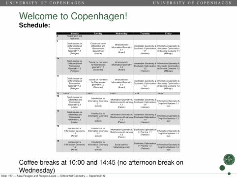
Welcome to Copenhagen!Schedule:
Monday Tuesday Wednesday Thursday Friday8 Registration and
welcome9
Crash course on Differential and
Riemannian Geometry 1.1
(Feragen)
Crash course on Differential and
Riemannian Geometry 3
(Lauze)
Introduction to Information Geometry
3.1(Amari)
Information Geometry & Stochastic Optimization
1.1(Hansen)
Information Geometry & Stochastic Optimization in Discrete Domains 1.1
(Màlago)
10Crash course on Differential and
Riemannian Geometry 1.2
(Feragen)
Tutorial on numerics for Riemannian
geometry 1.1(Sommer)
Introduction to Information Geometry
3.2(Amari)
Information Geometry & Stochastic Optimization
1.2(Hansen)
Information Geometry & Stochastic Optimization in Discrete Domains 1.2
(Màlago)
11Crash course on Differential and
Riemannian Geometry 1.3
(Feragen)
Tutorial on numerics for Riemannian
geometry 1.2(Sommer)
Introduction to Information Geometry
3.3(Amari)
Information Geometry & Stochastic Optimization
1.3(Hansen)
Information Geometry & Stochastic Optimization in Discrete Domains 1.3
(Màlago)
12 Lunch Lunch Lunch Lunch Lunch13 Crash course on
Differential and Riemannian
Geometry 2.1(Lauze)
Introduction to Information Geometry
2.1(Amari)
Information Geometry & Reinforcement Learning
1.1(Peters)
Information Geometry & Stochastic Optimization
1.4(Hansen)
Information Geometry & Cognitive Systems 1.1
(Ay)
14 Crash course on Differential and
RiemannianGeometry 2.2
(Lauze)
Introduction to Information Geometry
2.2(Amari)
Information Geometry & Reinforcement Learning
1.2(Peters)
Information Geometry & Stochastic Optimization
1.5(Hansen)
Information Geometry & Cognitive Systems 1.2
(Ay)
15Introduction to
Information Geometry 1.1
(Amari)
Introduction to Information Geometry
2.3(Amari)
Information Geometry & Reinforcement Learning
1.3(Peters)
Stochastic Optimization in Practice 1.1
(Hansen)
Information Geometry & Cognitive Systems 1.3
(Ay)
16 Introduction to Information Geometry
1.2(Amari)
Introduction to Information Geometry
2.4(Amari)
Social activity/Networking event
Stochastic Optimization in Practice 1.2
(Hansen)
Information Geometry & Cognitive Systems 1.3
(Ay)
Coffee breaks at 10:00 and 14:45 (no afternoon break onWednesday)
Slide 1/57 — Aasa Feragen and François Lauze — Differential Geometry — September 22
U N I V E R S I T Y O F C O P E N H A G E N U N I V E R S I T Y O F C O P E N H A G E N
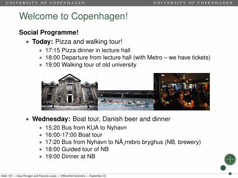
Welcome to Copenhagen!
Social Programme!• Today: Pizza and walking tour!
• 17:15 Pizza dinner in lecture hall• 18:00 Departure from lecture hall (with Metro – we have tickets)• 19:00 Walking tour of old university
• Wednesday: Boat tour, Danish beer and dinner• 15:20 Bus from KUA to Nyhavn• 16:00-17:00 Boat tour• 17:20 Bus from Nyhavn to Nørrebro bryghus (NB, brewery)• 18:00 Guided tour of NB• 19:00 Dinner at NB
Slide 1/57 — Aasa Feragen and François Lauze — Differential Geometry — September 22
U N I V E R S I T Y O F C O P E N H A G E N U N I V E R S I T Y O F C O P E N H A G E N
Welcome to Copenhagen!
• Lunch on your own – canteens and coffee on campus• Internet connection
• Eduroam• Alternative will be set up ASAP
• Emergency? Call Aasa: +4526220498• Questions?
Slide 1/57 — Aasa Feragen and François Lauze — Differential Geometry — September 22
U N I V E R S I T Y O F C O P E N H A G E N U N I V E R S I T Y O F C O P E N H A G E N
Faculty of Science
A Very Brief Introduction to Differentialand Riemannian Geometry
Aasa Feragen and François LauzeDepartment of Computer ScienceUniversity of Copenhagen
PhD course on Information geometry, Copenhagen 2014Slide 2/57
U N I V E R S I T Y O F C O P E N H A G E N U N I V E R S I T Y O F C O P E N H A G E N
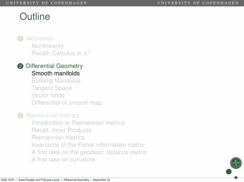
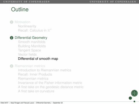
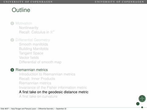
Outline
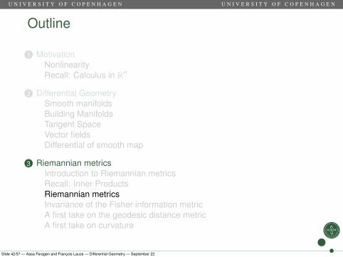
1 MotivationNonlinearityRecall: Calculus in Rn
2 Differential GeometrySmooth manifoldsBuilding ManifoldsTangent SpaceVector fieldsDifferential of smooth map
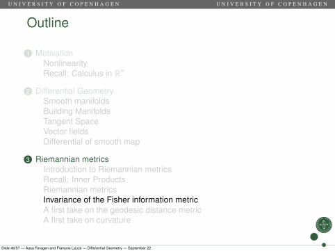
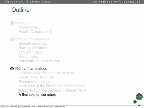
3 Riemannian metricsIntroduction to Riemannian metricsRecall: Inner ProductsRiemannian metricsInvariance of the Fisher information metricA first take on the geodesic distance metricA first take on curvature
Slide 3/57 — Aasa Feragen and François Lauze — Differential Geometry — September 22
U N I V E R S I T Y O F C O P E N H A G E N U N I V E R S I T Y O F C O P E N H A G E N
Outline
1 MotivationNonlinearityRecall: Calculus in Rn
2 Differential GeometrySmooth manifoldsBuilding ManifoldsTangent SpaceVector fieldsDifferential of smooth map
3 Riemannian metricsIntroduction to Riemannian metricsRecall: Inner ProductsRiemannian metricsInvariance of the Fisher information metricA first take on the geodesic distance metricA first take on curvature
Slide 4/57 — Aasa Feragen and François Lauze — Differential Geometry — September 22
U N I V E R S I T Y O F C O P E N H A G E N U N I V E R S I T Y O F C O P E N H A G E N
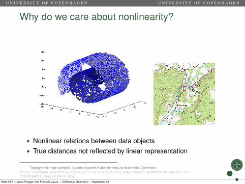
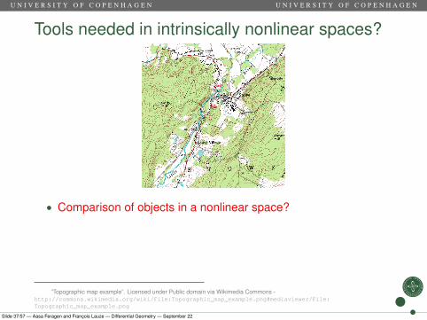
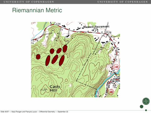
Why do we care about nonlinearity?
• Nonlinear relations between data objects• True distances not reflected by linear representation
”Topographic map example”. Licensed under Public domain via Wikimedia Commons -http://commons.wikimedia.org/wiki/File:Topographic_map_example.png#mediaviewer/File:Topographic_map_example.png
Slide 5/57 — Aasa Feragen and François Lauze — Differential Geometry — September 22
U N I V E R S I T Y O F C O P E N H A G E N U N I V E R S I T Y O F C O P E N H A G E N
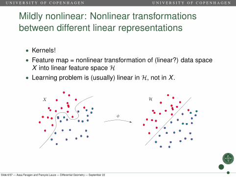
Mildly nonlinear: Nonlinear transformationsbetween different linear representations
• Kernels!• Feature map = nonlinear transformation of (linear?) data space
X into linear feature space H• Learning problem is (usually) linear in H, not in X .
Slide 6/57 — Aasa Feragen and François Lauze — Differential Geometry — September 22
U N I V E R S I T Y O F C O P E N H A G E N U N I V E R S I T Y O F C O P E N H A G E N
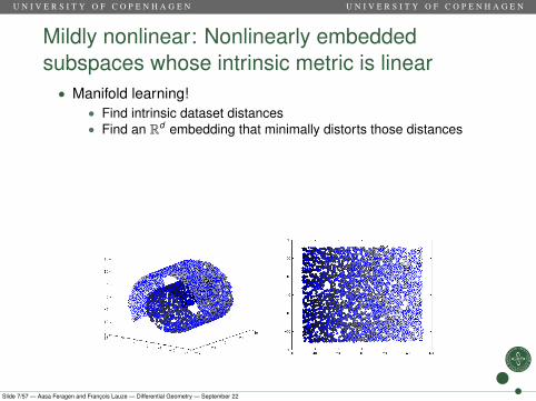
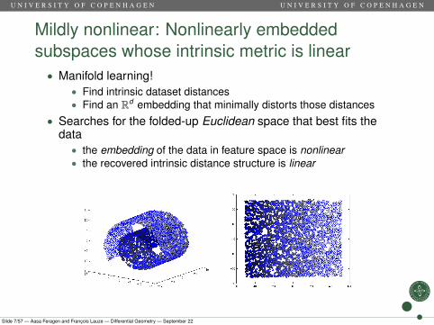
Mildly nonlinear: Nonlinearly embeddedsubspaces whose intrinsic metric is linear• Manifold learning!
• Find intrinsic dataset distances• Find an Rd embedding that minimally distorts those distances
• Searches for the folded-up Euclidean space that best fits thedata
• the embedding of the data in feature space is nonlinear• the recovered intrinsic distance structure is linear
Slide 7/57 — Aasa Feragen and François Lauze — Differential Geometry — September 22
U N I V E R S I T Y O F C O P E N H A G E N U N I V E R S I T Y O F C O P E N H A G E N
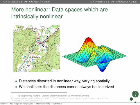
More nonlinear: Data spaces which areintrinsically nonlinear
• Distances distorted in nonlinear way, varying spatially• We shall see: the distances cannot always be linearized
”Topographic map example”. Licensed under Public domain via Wikimedia Commons -http://commons.wikimedia.org/wiki/File:Topographic_map_example.png#mediaviewer/File:Topographic_map_example.png
Slide 8/57 — Aasa Feragen and François Lauze — Differential Geometry — September 22
U N I V E R S I T Y O F C O P E N H A G E N U N I V E R S I T Y O F C O P E N H A G E N
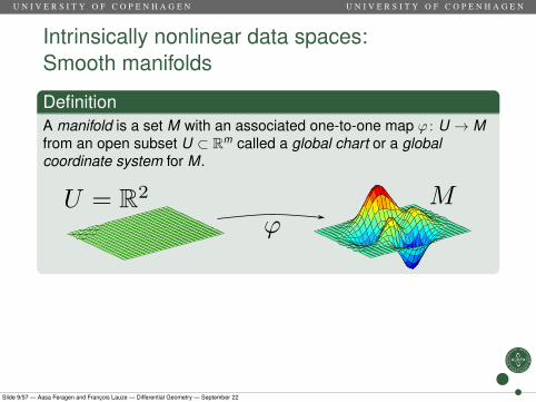
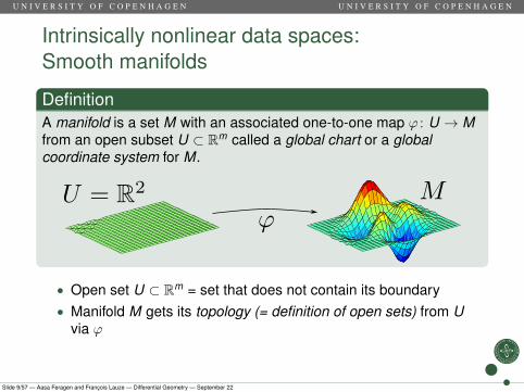
Intrinsically nonlinear data spaces:Smooth manifolds
DefinitionA manifold is a set M with an associated one-to-one map ϕ : U → Mfrom an open subset U ⊂ Rm called a global chart or a globalcoordinate system for M.
• Open set U ⊂ Rm = set that does not contain its boundary• Manifold M gets its topology (= definition of open sets) from U
via ϕ• What are the implications of getting the topology from U?
Slide 9/57 — Aasa Feragen and François Lauze — Differential Geometry — September 22
U N I V E R S I T Y O F C O P E N H A G E N U N I V E R S I T Y O F C O P E N H A G E N
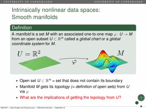
Intrinsically nonlinear data spaces:Smooth manifolds
DefinitionA manifold is a set M with an associated one-to-one map ϕ : U → Mfrom an open subset U ⊂ Rm called a global chart or a globalcoordinate system for M.
• Open set U ⊂ Rm = set that does not contain its boundary• Manifold M gets its topology (= definition of open sets) from U
via ϕ
• What are the implications of getting the topology from U?
Slide 9/57 — Aasa Feragen and François Lauze — Differential Geometry — September 22
U N I V E R S I T Y O F C O P E N H A G E N U N I V E R S I T Y O F C O P E N H A G E N
Intrinsically nonlinear data spaces:Smooth manifolds
DefinitionA manifold is a set M with an associated one-to-one map ϕ : U → Mfrom an open subset U ⊂ Rm called a global chart or a globalcoordinate system for M.
• Open set U ⊂ Rm = set that does not contain its boundary• Manifold M gets its topology (= definition of open sets) from U
via ϕ• What are the implications of getting the topology from U?
Slide 9/57 — Aasa Feragen and François Lauze — Differential Geometry — September 22
U N I V E R S I T Y O F C O P E N H A G E N U N I V E R S I T Y O F C O P E N H A G E N
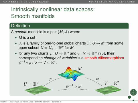
Intrinsically nonlinear data spaces:Smooth manifolds
DefinitionA smooth manifold is a pair (M,A) where• M is a set• A is a family of one-to-one global charts ϕ : U → M from some
open subset U = Uϕ ⊂ Rm for M,• for any two charts ϕ : U → Rm and ψ : V → Rm in A, their
corresponding change of variables is a smooth diffeomorphismψ−1 ◦ ϕ : U → V ⊂ Rm.
Slide 9/57 — Aasa Feragen and François Lauze — Differential Geometry — September 22
U N I V E R S I T Y O F C O P E N H A G E N U N I V E R S I T Y O F C O P E N H A G E N
Outline
1 MotivationNonlinearityRecall: Calculus in Rn
2 Differential GeometrySmooth manifoldsBuilding ManifoldsTangent SpaceVector fieldsDifferential of smooth map
3 Riemannian metricsIntroduction to Riemannian metricsRecall: Inner ProductsRiemannian metricsInvariance of the Fisher information metricA first take on the geodesic distance metricA first take on curvature
Slide 10/57 — Aasa Feragen and François Lauze — Differential Geometry — September 22
U N I V E R S I T Y O F C O P E N H A G E N U N I V E R S I T Y O F C O P E N H A G E N
Differentiable and smooth functions
• f : U open ⊂ Rn → Rq continuous: write
(y1, . . . , yq) = f (x1, . . . , xn)
• f is of class Cr if f has continuous partial derivatives
∂r1+···+rn yk
∂x r11 . . . ∂x rn
n
k = 1 . . . q, r1 + . . . rn ≤ r .• When r =∞, f is smooth. Our focus.
Slide 11/57 — Aasa Feragen and François Lauze — Differential Geometry — September 22
U N I V E R S I T Y O F C O P E N H A G E N U N I V E R S I T Y O F C O P E N H A G E N
Differentiable and smooth functions
• f : U open ⊂ Rn → Rq continuous: write
(y1, . . . , yq) = f (x1, . . . , xn)
• f is of class Cr if f has continuous partial derivatives
∂r1+···+rn yk
∂x r11 . . . ∂x rn
n
k = 1 . . . q, r1 + . . . rn ≤ r .
• When r =∞, f is smooth. Our focus.
Slide 11/57 — Aasa Feragen and François Lauze — Differential Geometry — September 22
U N I V E R S I T Y O F C O P E N H A G E N U N I V E R S I T Y O F C O P E N H A G E N
Differentiable and smooth functions
• f : U open ⊂ Rn → Rq continuous: write
(y1, . . . , yq) = f (x1, . . . , xn)
• f is of class Cr if f has continuous partial derivatives
∂r1+···+rn yk
∂x r11 . . . ∂x rn
n
k = 1 . . . q, r1 + . . . rn ≤ r .• When r =∞, f is smooth. Our focus.
Slide 11/57 — Aasa Feragen and François Lauze — Differential Geometry — September 22
U N I V E R S I T Y O F C O P E N H A G E N U N I V E R S I T Y O F C O P E N H A G E N
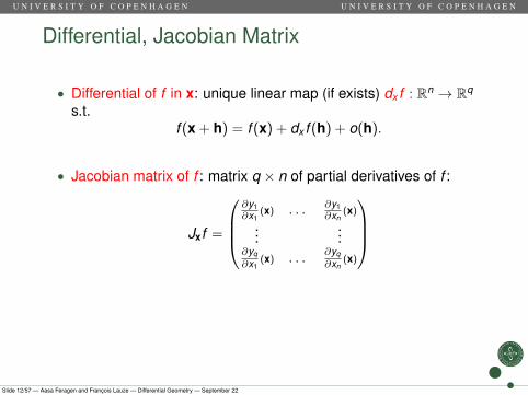
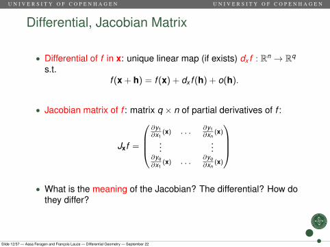
Differential, Jacobian Matrix
• Differential of f in x: unique linear map (if exists) dx f : Rn → Rq
s.t.f (x + h) = f (x) + dx f (h) + o(h).
• Jacobian matrix of f : matrix q × n of partial derivatives of f :
Jxf =
∂y1∂x1
(x) . . . ∂y1∂xn
(x)
......
∂yq∂x1
(x) . . .∂yq∂xn
(x)
• What is the meaning of the Jacobian? The differential? How do
they differ?
Slide 12/57 — Aasa Feragen and François Lauze — Differential Geometry — September 22
U N I V E R S I T Y O F C O P E N H A G E N U N I V E R S I T Y O F C O P E N H A G E N
Differential, Jacobian Matrix
• Differential of f in x: unique linear map (if exists) dx f : Rn → Rq
s.t.f (x + h) = f (x) + dx f (h) + o(h).
• Jacobian matrix of f : matrix q × n of partial derivatives of f :
Jxf =
∂y1∂x1
(x) . . . ∂y1∂xn
(x)
......
∂yq∂x1
(x) . . .∂yq∂xn
(x)
• What is the meaning of the Jacobian? The differential? How dothey differ?
Slide 12/57 — Aasa Feragen and François Lauze — Differential Geometry — September 22
U N I V E R S I T Y O F C O P E N H A G E N U N I V E R S I T Y O F C O P E N H A G E N
Differential, Jacobian Matrix
• Differential of f in x: unique linear map (if exists) dx f : Rn → Rq
s.t.f (x + h) = f (x) + dx f (h) + o(h).
• Jacobian matrix of f : matrix q × n of partial derivatives of f :
Jxf =
∂y1∂x1
(x) . . . ∂y1∂xn
(x)
......
∂yq∂x1
(x) . . .∂yq∂xn
(x)
• What is the meaning of the Jacobian? The differential? How do
they differ?
Slide 12/57 — Aasa Feragen and François Lauze — Differential Geometry — September 22
U N I V E R S I T Y O F C O P E N H A G E N U N I V E R S I T Y O F C O P E N H A G E N
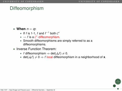
Diffeomorphism
• When n = q:• If f is 1-1, f and f−1 both Cr
• f is a Cr -diffeomorphism.• Smooth diffeomorphisms are simply referred to as a
diffeomorphisms.
• Inverse Function Theorem:• f diffeomorphism⇒ det(Jxf ) 6= 0.• det(Jxf ) 6= 0⇒ f local diffeomorphism in a neighborhood of x.
• What is the meaning of Jxf? Of det(Jxf ) 6= 0?
Slide 13/57 — Aasa Feragen and François Lauze — Differential Geometry — September 22
U N I V E R S I T Y O F C O P E N H A G E N U N I V E R S I T Y O F C O P E N H A G E N
Diffeomorphism
• When n = q:• If f is 1-1, f and f−1 both Cr
• f is a Cr -diffeomorphism.• Smooth diffeomorphisms are simply referred to as a
diffeomorphisms.• Inverse Function Theorem:
• f diffeomorphism⇒ det(Jxf ) 6= 0.• det(Jxf ) 6= 0⇒ f local diffeomorphism in a neighborhood of x.
• What is the meaning of Jxf? Of det(Jxf ) 6= 0?
Slide 13/57 — Aasa Feragen and François Lauze — Differential Geometry — September 22
U N I V E R S I T Y O F C O P E N H A G E N U N I V E R S I T Y O F C O P E N H A G E N
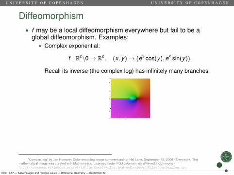
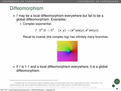
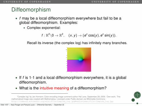
Diffeomorphism• f may be a local diffeomorphism everywhere but fail to be a
global diffeomorphism. Examples:• Complex exponential:
f : R2\0→ R2, (x , y)→ (ex cos(y), ex sin(y)).
Recall its inverse (the complex log) has infinitely many branches.
• If f is 1-1 and a local diffeomorphism everywhere, it is a globaldiffeomorphism.
• What is the intuitive meaning of a diffeomorphism?
”Complex log” by Jan Homann; Color encoding image comment author Hal Lane, September 28, 2009 - Own work. Thismathematical image was created with Mathematica. Licensed under Public domain via Wikimedia Commons -http://commons.wikimedia.org/wiki/File:Complex_log.jpg#mediaviewer/File:Complex_log.jpg
Slide 14/57 — Aasa Feragen and François Lauze — Differential Geometry — September 22
U N I V E R S I T Y O F C O P E N H A G E N U N I V E R S I T Y O F C O P E N H A G E N
Outline
1 MotivationNonlinearityRecall: Calculus in Rn
2 Differential GeometrySmooth manifoldsBuilding ManifoldsTangent SpaceVector fieldsDifferential of smooth map
3 Riemannian metricsIntroduction to Riemannian metricsRecall: Inner ProductsRiemannian metricsInvariance of the Fisher information metricA first take on the geodesic distance metricA first take on curvature
Slide 15/57 — Aasa Feragen and François Lauze — Differential Geometry — September 22
U N I V E R S I T Y O F C O P E N H A G E N U N I V E R S I T Y O F C O P E N H A G E N
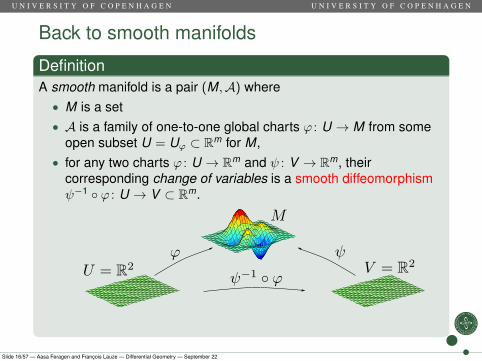
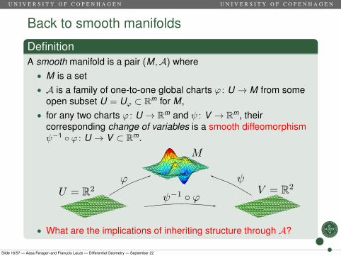
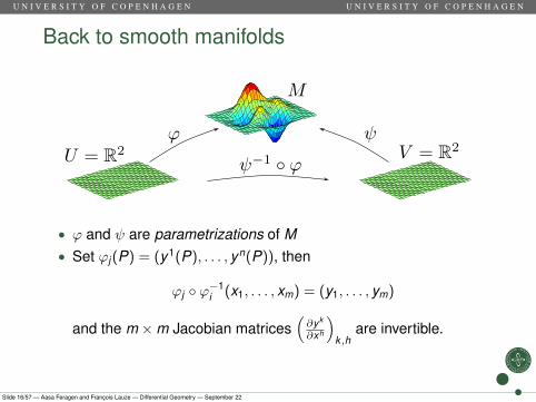
Back to smooth manifolds
DefinitionA smooth manifold is a pair (M,A) where• M is a set• A is a family of one-to-one global charts ϕ : U → M from some
open subset U = Uϕ ⊂ Rm for M,• for any two charts ϕ : U → Rm and ψ : V → Rm, their
corresponding change of variables is a smooth diffeomorphismψ−1 ◦ ϕ : U → V ⊂ Rm.
• What are the implications of inheriting structure through A?
Slide 16/57 — Aasa Feragen and François Lauze — Differential Geometry — September 22
U N I V E R S I T Y O F C O P E N H A G E N U N I V E R S I T Y O F C O P E N H A G E N
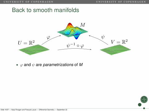
Back to smooth manifolds
• ϕ and ψ are parametrizations of M
• Set ϕj (P) = (y1(P), . . . , yn(P)), then
ϕj ◦ ϕ−1i (x1, . . . , xm) = (y1, . . . , ym)
and the m ×m Jacobian matrices(∂yk
∂xh
)k,h
are invertible.
Slide 16/57 — Aasa Feragen and François Lauze — Differential Geometry — September 22
U N I V E R S I T Y O F C O P E N H A G E N U N I V E R S I T Y O F C O P E N H A G E N
Back to smooth manifolds
• ϕ and ψ are parametrizations of M• Set ϕj (P) = (y1(P), . . . , yn(P)), then
ϕj ◦ ϕ−1i (x1, . . . , xm) = (y1, . . . , ym)
and the m ×m Jacobian matrices(∂yk
∂xh
)k,h
are invertible.
Slide 16/57 — Aasa Feragen and François Lauze — Differential Geometry — September 22
U N I V E R S I T Y O F C O P E N H A G E N U N I V E R S I T Y O F C O P E N H A G E N
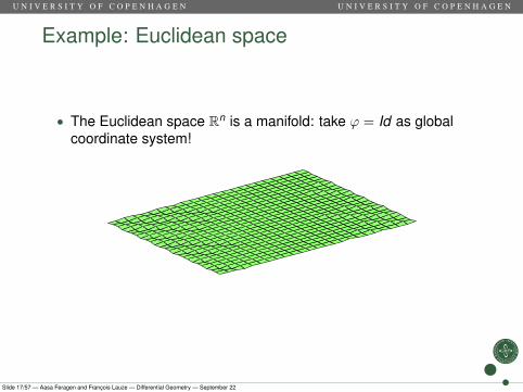
Example: Euclidean space
• The Euclidean space Rn is a manifold: take ϕ = Id as globalcoordinate system!
Slide 17/57 — Aasa Feragen and François Lauze — Differential Geometry — September 22
U N I V E R S I T Y O F C O P E N H A G E N U N I V E R S I T Y O F C O P E N H A G E N
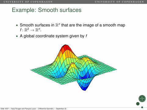
Example: Smooth surfaces
• Smooth surfaces in Rn that are the image of a smooth mapf : R2 → Rn.
• A global coordinate system given by f
Slide 18/57 — Aasa Feragen and François Lauze — Differential Geometry — September 22
U N I V E R S I T Y O F C O P E N H A G E N U N I V E R S I T Y O F C O P E N H A G E N
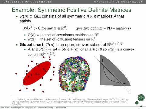
Example: Symmetric Positive Definite Matrices• P(n) ⊂ GLn consists of all symmetric n × n matrices A that
satisfy
xAxT > 0 for any x ∈ Rn, (positive definite – PD – matrices)
• P(n) = the set of covariance matrices on Rn
• P(3) = the set of (diffusion) tensors on R3
• Global chart: P(n) is an open, convex subset of R(n2+n)/2
• A,B ∈ P(n)→ aA + bB ∈ P(n) for all a, b > 0 so P(n) is a convexcone in R(n2+n)/2.
Middle figure from Fillard et al., A Riemannian Framework for the Processing of Tensor-Valued Images, LNCS 3753, 2005, pp112-123. Rightmost figure from Fletcher, Joshi, Principal Geodesic Analysis on Symmetric Spaces: Statistics of Diffusion Tensors,CVAMIA04
Slide 19/57 — Aasa Feragen and François Lauze — Differential Geometry — September 22
U N I V E R S I T Y O F C O P E N H A G E N U N I V E R S I T Y O F C O P E N H A G E N
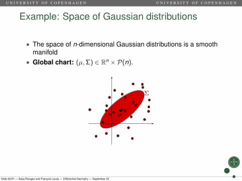
Example: Space of Gaussian distributions
• The space of n-dimensional Gaussian distributions is a smoothmanifold
• Global chart: (µ,Σ) ∈ Rn × P(n).
Slide 20/57 — Aasa Feragen and François Lauze — Differential Geometry — September 22
U N I V E R S I T Y O F C O P E N H A G E N U N I V E R S I T Y O F C O P E N H A G E N
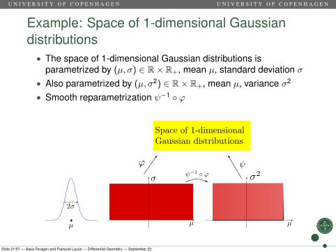
Example: Space of 1-dimensional Gaussiandistributions• The space of 1-dimensional Gaussian distributions is
parametrized by (µ, σ) ∈ R× R+, mean µ, standard deviation σ• Also parametrized by (µ, σ2) ∈ R× R+, mean µ, variance σ2
• Smooth reparametrization ψ−1 ◦ ϕ
Slide 21/57 — Aasa Feragen and François Lauze — Differential Geometry — September 22
U N I V E R S I T Y O F C O P E N H A G E N U N I V E R S I T Y O F C O P E N H A G E N
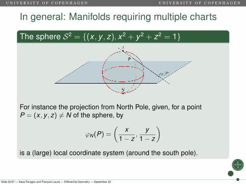
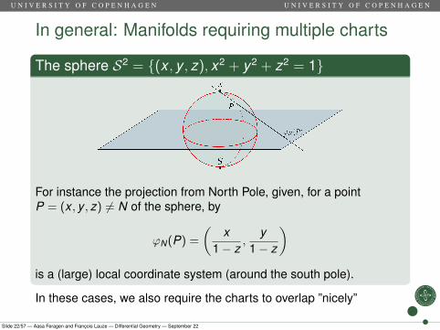
In general: Manifolds requiring multiple charts
The sphere S2 = {(x , y , z), x2 + y2 + z2 = 1}
For instance the projection from North Pole, given, for a pointP = (x , y , z) 6= N of the sphere, by
ϕN(P) =
(x
1− z,
y1− z
)is a (large) local coordinate system (around the south pole).
In these cases, we also require the charts to overlap ”nicely”
Slide 22/57 — Aasa Feragen and François Lauze — Differential Geometry — September 22
U N I V E R S I T Y O F C O P E N H A G E N U N I V E R S I T Y O F C O P E N H A G E N
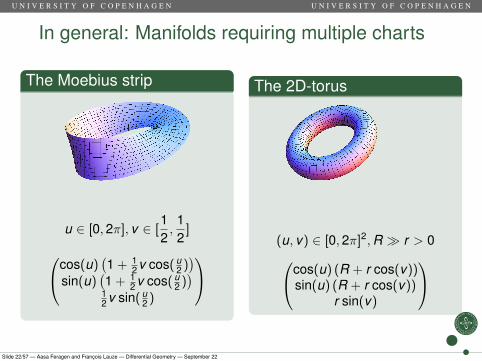
In general: Manifolds requiring multiple charts
The Moebius strip
u ∈ [0,2π], v ∈ [12,
12
]
cos(u)(1 + 1
2 v cos( u2 ))
sin(u)(1 + 1
2 v cos( u2 ))
12 v sin( u
2 )
The 2D-torus
(u, v) ∈ [0,2π]2,R � r > 0cos(u) (R + r cos(v))sin(u) (R + r cos(v))
r sin(v)
Slide 22/57 — Aasa Feragen and François Lauze — Differential Geometry — September 22

U N I V E R S I T Y O F C O P E N H A G E N U N I V E R S I T Y O F C O P E N H A G E N
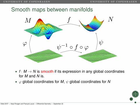
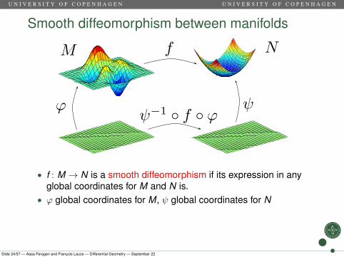
Smooth maps between manifolds
• f : M → N is smooth if its expression in any global coordinatesfor M and N is.
• ϕ global coordinates for M, ψ global coordinates for N
ϕ−1 ◦ f ◦ ψ smooth.
Slide 23/57 — Aasa Feragen and François Lauze — Differential Geometry — September 22
U N I V E R S I T Y O F C O P E N H A G E N U N I V E R S I T Y O F C O P E N H A G E N
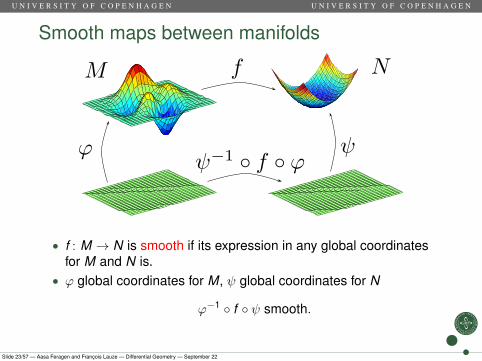
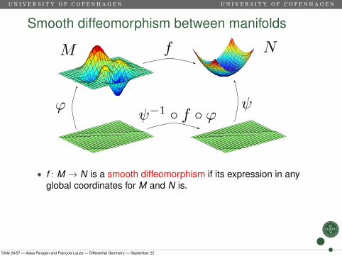
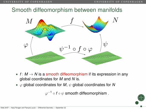
Smooth diffeomorphism between manifolds
• f : M → N is a smooth diffeomorphism if its expression in anyglobal coordinates for M and N is.
• ϕ global coordinates for M, ψ global coordinates for N
ϕ−1 ◦ f ◦ ψ smooth diffeomorphism .
Slide 24/57 — Aasa Feragen and François Lauze — Differential Geometry — September 22
U N I V E R S I T Y O F C O P E N H A G E N U N I V E R S I T Y O F C O P E N H A G E N
Outline
1 MotivationNonlinearityRecall: Calculus in Rn
2 Differential GeometrySmooth manifoldsBuilding ManifoldsTangent SpaceVector fieldsDifferential of smooth map
3 Riemannian metricsIntroduction to Riemannian metricsRecall: Inner ProductsRiemannian metricsInvariance of the Fisher information metricA first take on the geodesic distance metricA first take on curvature
Slide 25/57 — Aasa Feragen and François Lauze — Differential Geometry — September 22
U N I V E R S I T Y O F C O P E N H A G E N U N I V E R S I T Y O F C O P E N H A G E N
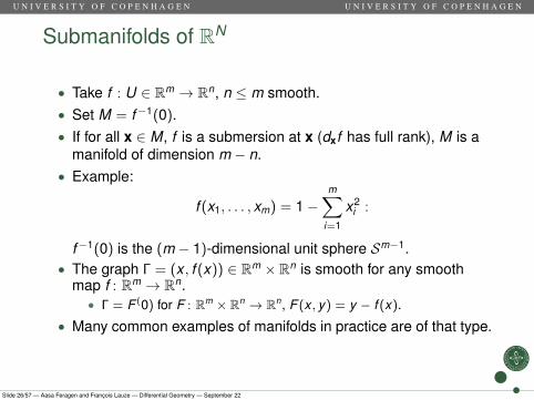
Submanifolds of RN
• Take f : U ∈ Rm → Rn, n ≤ m smooth.
• Set M = f−1(0).• If for all x ∈ M, f is a submersion at x (dxf has full rank), M is a
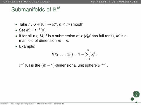
manifold of dimension m − n.• Example:
f (x1, . . . , xm) = 1−m∑
i=1
x2i :
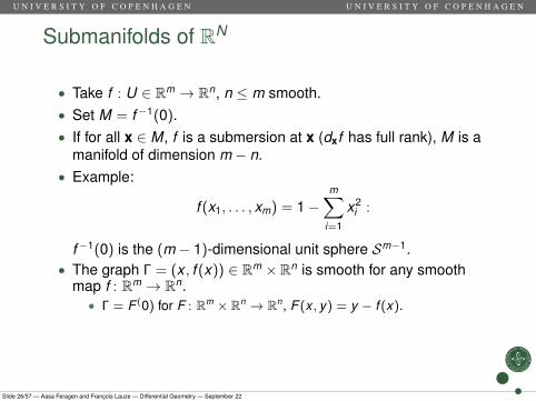
f−1(0) is the (m − 1)-dimensional unit sphere Sm−1.• The graph Γ = (x , f (x)) ∈ Rm × Rn is smooth for any smooth
map f : Rm → Rn.
• Γ = F (0) for F : Rm × Rn → Rn, F (x , y) = y − f (x).
• Many common examples of manifolds in practice are of that type.
Slide 26/57 — Aasa Feragen and François Lauze — Differential Geometry — September 22
U N I V E R S I T Y O F C O P E N H A G E N U N I V E R S I T Y O F C O P E N H A G E N
Submanifolds of RN
• Take f : U ∈ Rm → Rn, n ≤ m smooth.• Set M = f−1(0).
• If for all x ∈ M, f is a submersion at x (dxf has full rank), M is amanifold of dimension m − n.
• Example:
f (x1, . . . , xm) = 1−m∑
i=1
x2i :
f−1(0) is the (m − 1)-dimensional unit sphere Sm−1.• The graph Γ = (x , f (x)) ∈ Rm × Rn is smooth for any smooth
map f : Rm → Rn.
• Γ = F (0) for F : Rm × Rn → Rn, F (x , y) = y − f (x).
• Many common examples of manifolds in practice are of that type.
Slide 26/57 — Aasa Feragen and François Lauze — Differential Geometry — September 22
U N I V E R S I T Y O F C O P E N H A G E N U N I V E R S I T Y O F C O P E N H A G E N
Submanifolds of RN
• Take f : U ∈ Rm → Rn, n ≤ m smooth.• Set M = f−1(0).• If for all x ∈ M, f is a submersion at x (dxf has full rank), M is a
manifold of dimension m − n.
• Example:
f (x1, . . . , xm) = 1−m∑
i=1
x2i :
f−1(0) is the (m − 1)-dimensional unit sphere Sm−1.• The graph Γ = (x , f (x)) ∈ Rm × Rn is smooth for any smooth
map f : Rm → Rn.
• Γ = F (0) for F : Rm × Rn → Rn, F (x , y) = y − f (x).
• Many common examples of manifolds in practice are of that type.
Slide 26/57 — Aasa Feragen and François Lauze — Differential Geometry — September 22
U N I V E R S I T Y O F C O P E N H A G E N U N I V E R S I T Y O F C O P E N H A G E N
Submanifolds of RN
• Take f : U ∈ Rm → Rn, n ≤ m smooth.• Set M = f−1(0).• If for all x ∈ M, f is a submersion at x (dxf has full rank), M is a
manifold of dimension m − n.• Example:
f (x1, . . . , xm) = 1−m∑
i=1
x2i :
f−1(0) is the (m − 1)-dimensional unit sphere Sm−1.
• The graph Γ = (x , f (x)) ∈ Rm × Rn is smooth for any smoothmap f : Rm → Rn.
• Γ = F (0) for F : Rm × Rn → Rn, F (x , y) = y − f (x).
• Many common examples of manifolds in practice are of that type.
Slide 26/57 — Aasa Feragen and François Lauze — Differential Geometry — September 22

U N I V E R S I T Y O F C O P E N H A G E N U N I V E R S I T Y O F C O P E N H A G E N
Submanifolds of RN
• Take f : U ∈ Rm → Rn, n ≤ m smooth.• Set M = f−1(0).• If for all x ∈ M, f is a submersion at x (dxf has full rank), M is a
manifold of dimension m − n.• Example:
f (x1, . . . , xm) = 1−m∑
i=1
x2i :
f−1(0) is the (m − 1)-dimensional unit sphere Sm−1.• The graph Γ = (x , f (x)) ∈ Rm × Rn is smooth for any smooth
map f : Rm → Rn.
• Γ = F (0) for F : Rm × Rn → Rn, F (x , y) = y − f (x).
• Many common examples of manifolds in practice are of that type.
Slide 26/57 — Aasa Feragen and François Lauze — Differential Geometry — September 22
U N I V E R S I T Y O F C O P E N H A G E N U N I V E R S I T Y O F C O P E N H A G E N
Submanifolds of RN
• Take f : U ∈ Rm → Rn, n ≤ m smooth.• Set M = f−1(0).• If for all x ∈ M, f is a submersion at x (dxf has full rank), M is a
manifold of dimension m − n.• Example:
f (x1, . . . , xm) = 1−m∑
i=1
x2i :
f−1(0) is the (m − 1)-dimensional unit sphere Sm−1.• The graph Γ = (x , f (x)) ∈ Rm × Rn is smooth for any smooth
map f : Rm → Rn.• Γ = F (0) for F : Rm × Rn → Rn, F (x , y) = y − f (x).
• Many common examples of manifolds in practice are of that type.
Slide 26/57 — Aasa Feragen and François Lauze — Differential Geometry — September 22
U N I V E R S I T Y O F C O P E N H A G E N U N I V E R S I T Y O F C O P E N H A G E N
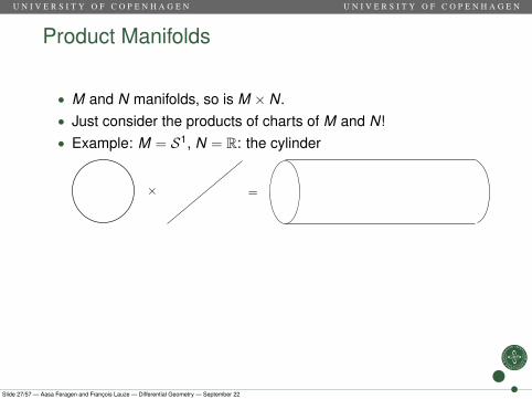
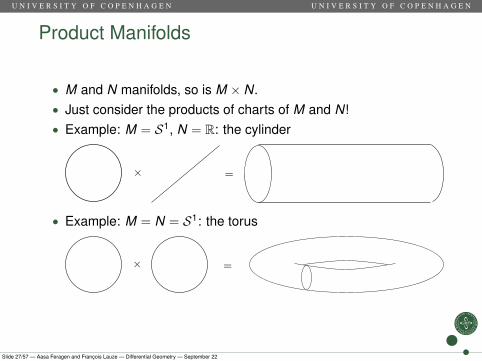
Product Manifolds
• M and N manifolds, so is M × N.
• Just consider the products of charts of M and N!• Example: M = S1, N = R: the cylinder
• Example: M = N = S1: the torus
Slide 27/57 — Aasa Feragen and François Lauze — Differential Geometry — September 22
U N I V E R S I T Y O F C O P E N H A G E N U N I V E R S I T Y O F C O P E N H A G E N
Product Manifolds
• M and N manifolds, so is M × N.• Just consider the products of charts of M and N!
• Example: M = S1, N = R: the cylinder
• Example: M = N = S1: the torus
Slide 27/57 — Aasa Feragen and François Lauze — Differential Geometry — September 22
U N I V E R S I T Y O F C O P E N H A G E N U N I V E R S I T Y O F C O P E N H A G E N
Product Manifolds
• M and N manifolds, so is M × N.• Just consider the products of charts of M and N!• Example: M = S1, N = R: the cylinder
• Example: M = N = S1: the torus
Slide 27/57 — Aasa Feragen and François Lauze — Differential Geometry — September 22
U N I V E R S I T Y O F C O P E N H A G E N U N I V E R S I T Y O F C O P E N H A G E N
Outline
1 MotivationNonlinearityRecall: Calculus in Rn
2 Differential GeometrySmooth manifoldsBuilding ManifoldsTangent SpaceVector fieldsDifferential of smooth map
3 Riemannian metricsIntroduction to Riemannian metricsRecall: Inner ProductsRiemannian metricsInvariance of the Fisher information metricA first take on the geodesic distance metricA first take on curvature
Slide 28/57 — Aasa Feragen and François Lauze — Differential Geometry — September 22

U N I V E R S I T Y O F C O P E N H A G E N U N I V E R S I T Y O F C O P E N H A G E N
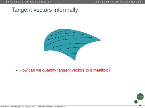
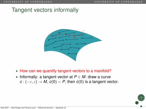
Tangent vectors informally
• How can we quantify tangent vectors to a manifold?
• Informally: a tangent vector at P ∈ M: draw a curvec : (−ε, ε)→ M, c(0) = P, then c(0) is a tangent vector.
Slide 29/57 — Aasa Feragen and François Lauze — Differential Geometry — September 22
U N I V E R S I T Y O F C O P E N H A G E N U N I V E R S I T Y O F C O P E N H A G E N
Tangent vectors informally
• How can we quantify tangent vectors to a manifold?• Informally: a tangent vector at P ∈ M: draw a curve
c : (−ε, ε)→ M, c(0) = P, then c(0) is a tangent vector.
Slide 29/57 — Aasa Feragen and François Lauze — Differential Geometry — September 22
U N I V E R S I T Y O F C O P E N H A G E N U N I V E R S I T Y O F C O P E N H A G E N
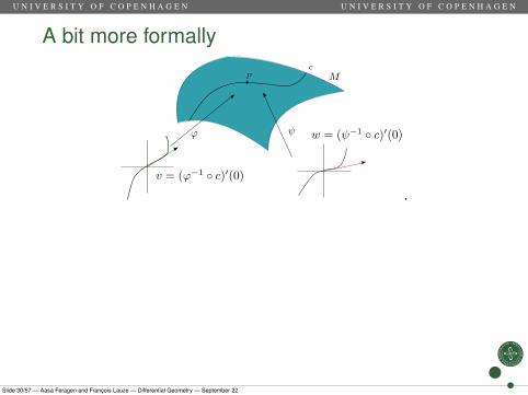
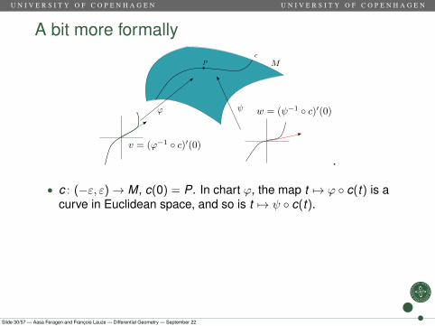
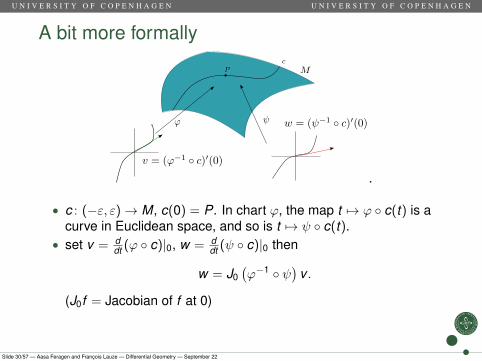
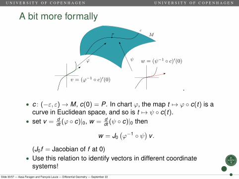
A bit more formally
.
• c : (−ε, ε)→ M, c(0) = P. In chart ϕ, the map t 7→ ϕ ◦ c(t) is acurve in Euclidean space, and so is t 7→ ψ ◦ c(t).
• set v = ddt (ϕ ◦ c)|0, w = d
dt (ψ ◦ c)|0 then
w = J0(ϕ−1 ◦ ψ
)v .
(J0f = Jacobian of f at 0)• Use this relation to identify vectors in different coordinate
systems!
Slide 30/57 — Aasa Feragen and François Lauze — Differential Geometry — September 22
U N I V E R S I T Y O F C O P E N H A G E N U N I V E R S I T Y O F C O P E N H A G E N
A bit more formally
.
• c : (−ε, ε)→ M, c(0) = P. In chart ϕ, the map t 7→ ϕ ◦ c(t) is acurve in Euclidean space, and so is t 7→ ψ ◦ c(t).
• set v = ddt (ϕ ◦ c)|0, w = d
dt (ψ ◦ c)|0 then
w = J0(ϕ−1 ◦ ψ
)v .
(J0f = Jacobian of f at 0)
• Use this relation to identify vectors in different coordinatesystems!
Slide 30/57 — Aasa Feragen and François Lauze — Differential Geometry — September 22
U N I V E R S I T Y O F C O P E N H A G E N U N I V E R S I T Y O F C O P E N H A G E N
A bit more formally
.
• c : (−ε, ε)→ M, c(0) = P. In chart ϕ, the map t 7→ ϕ ◦ c(t) is acurve in Euclidean space, and so is t 7→ ψ ◦ c(t).
• set v = ddt (ϕ ◦ c)|0, w = d
dt (ψ ◦ c)|0 then
w = J0(ϕ−1 ◦ ψ
)v .
(J0f = Jacobian of f at 0)• Use this relation to identify vectors in different coordinate
systems!Slide 30/57 — Aasa Feragen and François Lauze — Differential Geometry — September 22
U N I V E R S I T Y O F C O P E N H A G E N U N I V E R S I T Y O F C O P E N H A G E N
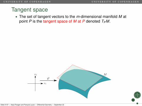
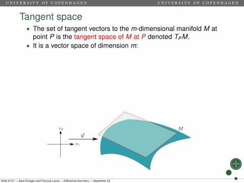
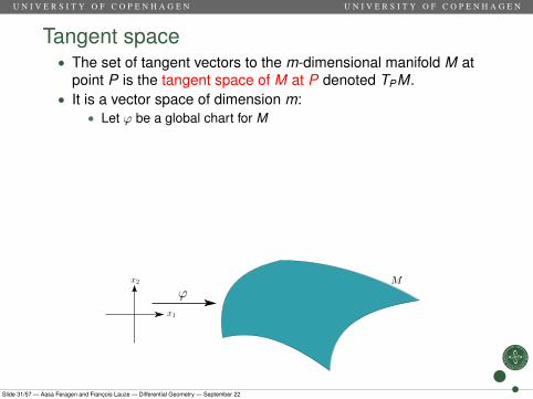
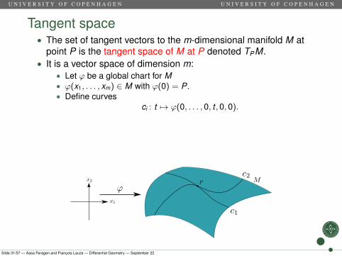
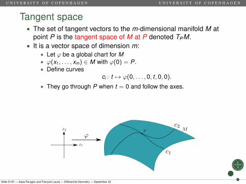
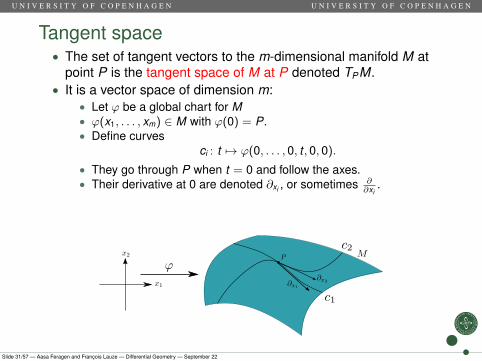
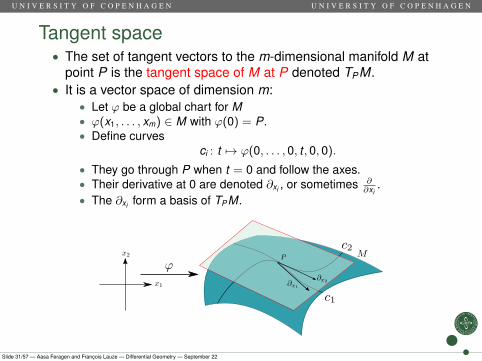
Tangent space• The set of tangent vectors to the m-dimensional manifold M at
point P is the tangent space of M at P denoted TPM.
• It is a vector space of dimension m:
• Let ϕ be a global chart for M• ϕ(x1, . . . , xm) ∈ M with ϕ(0) = P.• Define curves
ci : t 7→ ϕ(0, . . . , 0, t , 0, 0).
• They go through P when t = 0 and follow the axes.• Their derivative at 0 are denoted ∂xi , or sometimes ∂
∂xi.
• The ∂xi form a basis of TPM.
Slide 31/57 — Aasa Feragen and François Lauze — Differential Geometry — September 22
U N I V E R S I T Y O F C O P E N H A G E N U N I V E R S I T Y O F C O P E N H A G E N
Tangent space• The set of tangent vectors to the m-dimensional manifold M at
point P is the tangent space of M at P denoted TPM.• It is a vector space of dimension m:
• Let ϕ be a global chart for M
• ϕ(x1, . . . , xm) ∈ M with ϕ(0) = P.• Define curves
ci : t 7→ ϕ(0, . . . , 0, t , 0, 0).
• They go through P when t = 0 and follow the axes.• Their derivative at 0 are denoted ∂xi , or sometimes ∂
∂xi.
• The ∂xi form a basis of TPM.
Slide 31/57 — Aasa Feragen and François Lauze — Differential Geometry — September 22

U N I V E R S I T Y O F C O P E N H A G E N U N I V E R S I T Y O F C O P E N H A G E N
Tangent space• The set of tangent vectors to the m-dimensional manifold M at
point P is the tangent space of M at P denoted TPM.• It is a vector space of dimension m:
• Let ϕ be a global chart for M• ϕ(x1, . . . , xm) ∈ M with ϕ(0) = P.
• Define curvesci : t 7→ ϕ(0, . . . , 0, t , 0, 0).
• They go through P when t = 0 and follow the axes.• Their derivative at 0 are denoted ∂xi , or sometimes ∂
∂xi.
• The ∂xi form a basis of TPM.
Slide 31/57 — Aasa Feragen and François Lauze — Differential Geometry — September 22
U N I V E R S I T Y O F C O P E N H A G E N U N I V E R S I T Y O F C O P E N H A G E N
Tangent space• The set of tangent vectors to the m-dimensional manifold M at
point P is the tangent space of M at P denoted TPM.• It is a vector space of dimension m:
• Let ϕ be a global chart for M• ϕ(x1, . . . , xm) ∈ M with ϕ(0) = P.• Define curves
ci : t 7→ ϕ(0, . . . , 0, t , 0, 0).
• They go through P when t = 0 and follow the axes.• Their derivative at 0 are denoted ∂xi , or sometimes ∂
∂xi.
• The ∂xi form a basis of TPM.
Slide 31/57 — Aasa Feragen and François Lauze — Differential Geometry — September 22
U N I V E R S I T Y O F C O P E N H A G E N U N I V E R S I T Y O F C O P E N H A G E N
Tangent space• The set of tangent vectors to the m-dimensional manifold M at
point P is the tangent space of M at P denoted TPM.• It is a vector space of dimension m:
• Let ϕ be a global chart for M• ϕ(x1, . . . , xm) ∈ M with ϕ(0) = P.• Define curves
ci : t 7→ ϕ(0, . . . , 0, t , 0, 0).
• They go through P when t = 0 and follow the axes.
• Their derivative at 0 are denoted ∂xi , or sometimes ∂∂xi
.• The ∂xi form a basis of TPM.
Slide 31/57 — Aasa Feragen and François Lauze — Differential Geometry — September 22
U N I V E R S I T Y O F C O P E N H A G E N U N I V E R S I T Y O F C O P E N H A G E N
Tangent space• The set of tangent vectors to the m-dimensional manifold M at
point P is the tangent space of M at P denoted TPM.• It is a vector space of dimension m:
• Let ϕ be a global chart for M• ϕ(x1, . . . , xm) ∈ M with ϕ(0) = P.• Define curves
ci : t 7→ ϕ(0, . . . , 0, t , 0, 0).
• They go through P when t = 0 and follow the axes.• Their derivative at 0 are denoted ∂xi , or sometimes ∂
∂xi.
• The ∂xi form a basis of TPM.
Slide 31/57 — Aasa Feragen and François Lauze — Differential Geometry — September 22
U N I V E R S I T Y O F C O P E N H A G E N U N I V E R S I T Y O F C O P E N H A G E N
Tangent space• The set of tangent vectors to the m-dimensional manifold M at
point P is the tangent space of M at P denoted TPM.• It is a vector space of dimension m:
• Let ϕ be a global chart for M• ϕ(x1, . . . , xm) ∈ M with ϕ(0) = P.• Define curves
ci : t 7→ ϕ(0, . . . , 0, t , 0, 0).
• They go through P when t = 0 and follow the axes.• Their derivative at 0 are denoted ∂xi , or sometimes ∂
∂xi.
• The ∂xi form a basis of TPM.
Slide 31/57 — Aasa Feragen and François Lauze — Differential Geometry — September 22
U N I V E R S I T Y O F C O P E N H A G E N U N I V E R S I T Y O F C O P E N H A G E N
Outline
1 MotivationNonlinearityRecall: Calculus in Rn
2 Differential GeometrySmooth manifoldsBuilding ManifoldsTangent SpaceVector fieldsDifferential of smooth map
3 Riemannian metricsIntroduction to Riemannian metricsRecall: Inner ProductsRiemannian metricsInvariance of the Fisher information metricA first take on the geodesic distance metricA first take on curvature
Slide 32/57 — Aasa Feragen and François Lauze — Differential Geometry — September 22

U N I V E R S I T Y O F C O P E N H A G E N U N I V E R S I T Y O F C O P E N H A G E N
Vector fields
• A vector field is a smooth map that sends P ∈ M to a vectorv(P) ∈ TPM.
Slide 33/57 — Aasa Feragen and François Lauze — Differential Geometry — September 22
U N I V E R S I T Y O F C O P E N H A G E N U N I V E R S I T Y O F C O P E N H A G E N
Outline
1 MotivationNonlinearityRecall: Calculus in Rn
2 Differential GeometrySmooth manifoldsBuilding ManifoldsTangent SpaceVector fieldsDifferential of smooth map
3 Riemannian metricsIntroduction to Riemannian metricsRecall: Inner ProductsRiemannian metricsInvariance of the Fisher information metricA first take on the geodesic distance metricA first take on curvature
Slide 34/57 — Aasa Feragen and François Lauze — Differential Geometry — September 22
U N I V E R S I T Y O F C O P E N H A G E N U N I V E R S I T Y O F C O P E N H A G E N
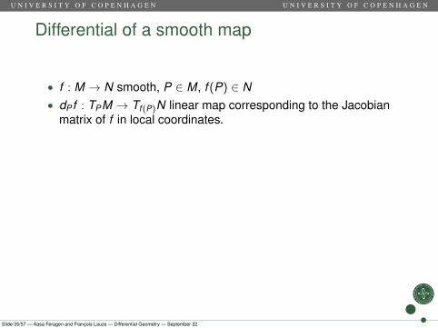
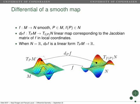
Differential of a smooth map
• f : M → N smooth, P ∈ M, f (P) ∈ N
• dP f : TPM → Tf (P)N linear map corresponding to the Jacobianmatrix of f in local coordinates.
• When N = R, dP f is a linear form TPM → R.
Slide 35/57 — Aasa Feragen and François Lauze — Differential Geometry — September 22
U N I V E R S I T Y O F C O P E N H A G E N U N I V E R S I T Y O F C O P E N H A G E N
Differential of a smooth map
• f : M → N smooth, P ∈ M, f (P) ∈ N• dP f : TPM → Tf (P)N linear map corresponding to the Jacobian
matrix of f in local coordinates.
• When N = R, dP f is a linear form TPM → R.
Slide 35/57 — Aasa Feragen and François Lauze — Differential Geometry — September 22
U N I V E R S I T Y O F C O P E N H A G E N U N I V E R S I T Y O F C O P E N H A G E N
Differential of a smooth map
• f : M → N smooth, P ∈ M, f (P) ∈ N• dP f : TPM → Tf (P)N linear map corresponding to the Jacobian
matrix of f in local coordinates.• When N = R, dP f is a linear form TPM → R.
Slide 35/57 — Aasa Feragen and François Lauze — Differential Geometry — September 22
U N I V E R S I T Y O F C O P E N H A G E N U N I V E R S I T Y O F C O P E N H A G E N
Outline
1 MotivationNonlinearityRecall: Calculus in Rn
2 Differential GeometrySmooth manifoldsBuilding ManifoldsTangent SpaceVector fieldsDifferential of smooth map
3 Riemannian metricsIntroduction to Riemannian metricsRecall: Inner ProductsRiemannian metricsInvariance of the Fisher information metricA first take on the geodesic distance metricA first take on curvature
Slide 36/57 — Aasa Feragen and François Lauze — Differential Geometry — September 22
U N I V E R S I T Y O F C O P E N H A G E N U N I V E R S I T Y O F C O P E N H A G E N
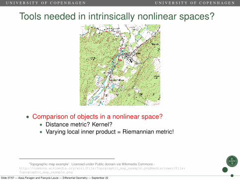
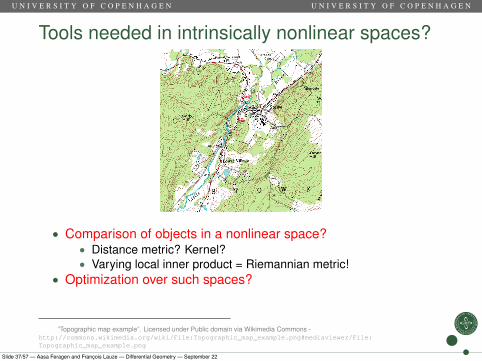
Tools needed in intrinsically nonlinear spaces?
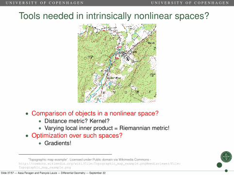
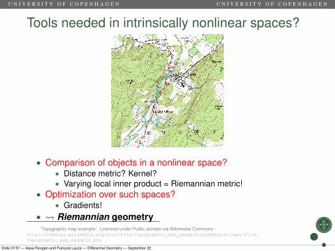
• Comparison of objects in a nonlinear space?
• Distance metric? Kernel?• Varying local inner product = Riemannian metric!
• Optimization over such spaces?
• Gradients!
• Riemannian geometry
”Topographic map example”. Licensed under Public domain via Wikimedia Commons -http://commons.wikimedia.org/wiki/File:Topographic_map_example.png#mediaviewer/File:Topographic_map_example.png
Slide 37/57 — Aasa Feragen and François Lauze — Differential Geometry — September 22
U N I V E R S I T Y O F C O P E N H A G E N U N I V E R S I T Y O F C O P E N H A G E N
Tools needed in intrinsically nonlinear spaces?
• Comparison of objects in a nonlinear space?• Distance metric? Kernel?• Varying local inner product = Riemannian metric!
• Optimization over such spaces?
• Gradients!• Riemannian geometry
”Topographic map example”. Licensed under Public domain via Wikimedia Commons -http://commons.wikimedia.org/wiki/File:Topographic_map_example.png#mediaviewer/File:Topographic_map_example.png
Slide 37/57 — Aasa Feragen and François Lauze — Differential Geometry — September 22
U N I V E R S I T Y O F C O P E N H A G E N U N I V E R S I T Y O F C O P E N H A G E N
Tools needed in intrinsically nonlinear spaces?
• Comparison of objects in a nonlinear space?• Distance metric? Kernel?• Varying local inner product = Riemannian metric!
• Optimization over such spaces?• Gradients!
• Riemannian geometry
”Topographic map example”. Licensed under Public domain via Wikimedia Commons -http://commons.wikimedia.org/wiki/File:Topographic_map_example.png#mediaviewer/File:Topographic_map_example.png
Slide 37/57 — Aasa Feragen and François Lauze — Differential Geometry — September 22
U N I V E R S I T Y O F C O P E N H A G E N U N I V E R S I T Y O F C O P E N H A G E N
Tools needed in intrinsically nonlinear spaces?
• Comparison of objects in a nonlinear space?• Distance metric? Kernel?• Varying local inner product = Riemannian metric!
• Optimization over such spaces?• Gradients!
• Riemannian geometry”Topographic map example”. Licensed under Public domain via Wikimedia Commons -
http://commons.wikimedia.org/wiki/File:Topographic_map_example.png#mediaviewer/File:Topographic_map_example.png
Slide 37/57 — Aasa Feragen and François Lauze — Differential Geometry — September 22
U N I V E R S I T Y O F C O P E N H A G E N U N I V E R S I T Y O F C O P E N H A G E N
Outline
1 MotivationNonlinearityRecall: Calculus in Rn
2 Differential GeometrySmooth manifoldsBuilding ManifoldsTangent SpaceVector fieldsDifferential of smooth map
3 Riemannian metricsIntroduction to Riemannian metricsRecall: Inner ProductsRiemannian metricsInvariance of the Fisher information metricA first take on the geodesic distance metricA first take on curvature
Slide 38/57 — Aasa Feragen and François Lauze — Differential Geometry — September 22
U N I V E R S I T Y O F C O P E N H A G E N U N I V E R S I T Y O F C O P E N H A G E N
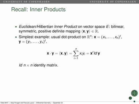
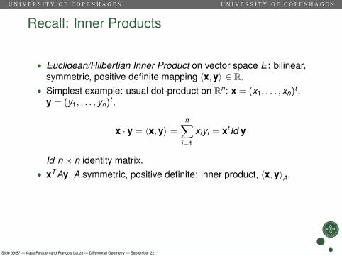
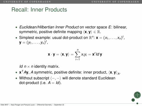
Recall: Inner Products
• Euclidean/Hilbertian Inner Product on vector space E : bilinear,symmetric, positive definite mapping 〈x,y〉 ∈ R.
• Simplest example: usual dot-product on Rn: x = (x1, . . . , xn)t ,y = (y1, . . . , yn)t ,
x · y = 〈x,y〉 =n∑
i=1
xiyi = xt Id y
Id n × n identity matrix.• xT Ay, A symmetric, positive definite: inner product, 〈x,y〉A.• Without subscript 〈−,−〉 will denote standard Euclidean
dot-product (i.e. A = Id).
Slide 39/57 — Aasa Feragen and François Lauze — Differential Geometry — September 22
U N I V E R S I T Y O F C O P E N H A G E N U N I V E R S I T Y O F C O P E N H A G E N
Recall: Inner Products
• Euclidean/Hilbertian Inner Product on vector space E : bilinear,symmetric, positive definite mapping 〈x,y〉 ∈ R.
• Simplest example: usual dot-product on Rn: x = (x1, . . . , xn)t ,y = (y1, . . . , yn)t ,
x · y = 〈x,y〉 =n∑
i=1
xiyi = xt Id y
Id n × n identity matrix.
• xT Ay, A symmetric, positive definite: inner product, 〈x,y〉A.• Without subscript 〈−,−〉 will denote standard Euclidean
dot-product (i.e. A = Id).
Slide 39/57 — Aasa Feragen and François Lauze — Differential Geometry — September 22
U N I V E R S I T Y O F C O P E N H A G E N U N I V E R S I T Y O F C O P E N H A G E N
Recall: Inner Products
• Euclidean/Hilbertian Inner Product on vector space E : bilinear,symmetric, positive definite mapping 〈x,y〉 ∈ R.
• Simplest example: usual dot-product on Rn: x = (x1, . . . , xn)t ,y = (y1, . . . , yn)t ,
x · y = 〈x,y〉 =n∑
i=1
xiyi = xt Id y
Id n × n identity matrix.• xT Ay, A symmetric, positive definite: inner product, 〈x,y〉A.
• Without subscript 〈−,−〉 will denote standard Euclideandot-product (i.e. A = Id).
Slide 39/57 — Aasa Feragen and François Lauze — Differential Geometry — September 22
U N I V E R S I T Y O F C O P E N H A G E N U N I V E R S I T Y O F C O P E N H A G E N
Recall: Inner Products
• Euclidean/Hilbertian Inner Product on vector space E : bilinear,symmetric, positive definite mapping 〈x,y〉 ∈ R.
• Simplest example: usual dot-product on Rn: x = (x1, . . . , xn)t ,y = (y1, . . . , yn)t ,
x · y = 〈x,y〉 =n∑
i=1
xiyi = xt Id y
Id n × n identity matrix.• xT Ay, A symmetric, positive definite: inner product, 〈x,y〉A.• Without subscript 〈−,−〉 will denote standard Euclidean
dot-product (i.e. A = Id).
Slide 39/57 — Aasa Feragen and François Lauze — Differential Geometry — September 22
U N I V E R S I T Y O F C O P E N H A G E N U N I V E R S I T Y O F C O P E N H A G E N
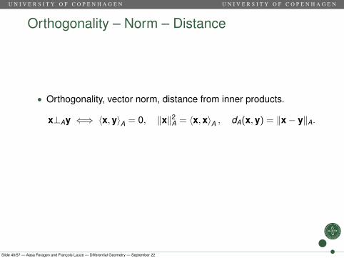
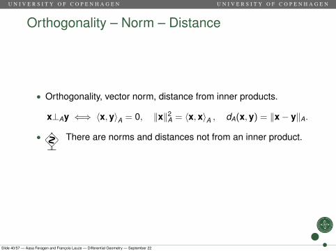
Orthogonality – Norm – Distance
• Orthogonality, vector norm, distance from inner products.
x⊥Ay ⇐⇒ 〈x,y〉A = 0, ‖x‖2A = 〈x,x〉A , dA(x,y) = ‖x− y‖A.
• � There are norms and distances not from an inner product.
Slide 40/57 — Aasa Feragen and François Lauze — Differential Geometry — September 22
U N I V E R S I T Y O F C O P E N H A G E N U N I V E R S I T Y O F C O P E N H A G E N
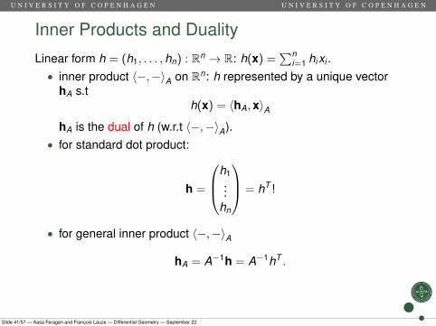
Inner Products and Duality
Linear form h = (h1, . . . ,hn) : Rn → R: h(x) =∑n
i=1 hixi .• inner product 〈−,−〉A on Rn: h represented by a unique vector
hA s.th(x) = 〈hA,x〉A
hA is the dual of h (w.r.t 〈−,−〉A).
• for standard dot product:
h =
h1...
hn
= hT !
• for general inner product 〈−,−〉A
hA = A−1h = A−1hT .
Slide 41/57 — Aasa Feragen and François Lauze — Differential Geometry — September 22
U N I V E R S I T Y O F C O P E N H A G E N U N I V E R S I T Y O F C O P E N H A G E N
Inner Products and Duality
Linear form h = (h1, . . . ,hn) : Rn → R: h(x) =∑n
i=1 hixi .• inner product 〈−,−〉A on Rn: h represented by a unique vector
hA s.th(x) = 〈hA,x〉A
hA is the dual of h (w.r.t 〈−,−〉A).• for standard dot product:
h =
h1...
hn
= hT !
• for general inner product 〈−,−〉A
hA = A−1h = A−1hT .
Slide 41/57 — Aasa Feragen and François Lauze — Differential Geometry — September 22
U N I V E R S I T Y O F C O P E N H A G E N U N I V E R S I T Y O F C O P E N H A G E N
Outline
1 MotivationNonlinearityRecall: Calculus in Rn
2 Differential GeometrySmooth manifoldsBuilding ManifoldsTangent SpaceVector fieldsDifferential of smooth map
3 Riemannian metricsIntroduction to Riemannian metricsRecall: Inner ProductsRiemannian metricsInvariance of the Fisher information metricA first take on the geodesic distance metricA first take on curvature
Slide 42/57 — Aasa Feragen and François Lauze — Differential Geometry — September 22
U N I V E R S I T Y O F C O P E N H A G E N U N I V E R S I T Y O F C O P E N H A G E N
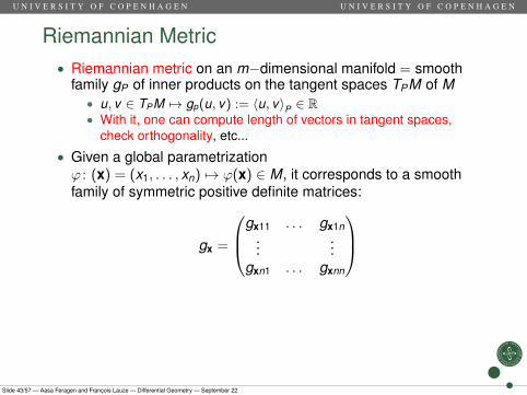
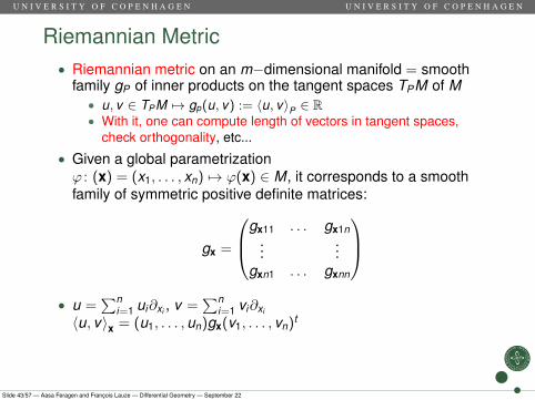
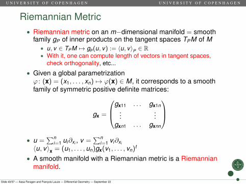
Riemannian Metric• Riemannian metric on an m−dimensional manifold = smooth
family gP of inner products on the tangent spaces TPM of M• u, v ∈ TPM 7→ gp(u, v) := 〈u, v〉P ∈ R• With it, one can compute length of vectors in tangent spaces,
check orthogonality, etc...
• Given a global parametrizationϕ : (x) = (x1, . . . , xn) 7→ ϕ(x) ∈ M, it corresponds to a smoothfamily of symmetric positive definite matrices:
gx =
gx11 . . . gx1n...
...gxn1 . . . gxnn
• u =
∑ni=1 ui∂xi , v =
∑ni=1 vi∂xi
〈u, v〉x = (u1, . . . ,un)gx(v1, . . . , vn)t
• A smooth manifold with a Riemannian metric is a Riemannianmanifold.
Slide 43/57 — Aasa Feragen and François Lauze — Differential Geometry — September 22
U N I V E R S I T Y O F C O P E N H A G E N U N I V E R S I T Y O F C O P E N H A G E N
Riemannian Metric• Riemannian metric on an m−dimensional manifold = smooth
family gP of inner products on the tangent spaces TPM of M• u, v ∈ TPM 7→ gp(u, v) := 〈u, v〉P ∈ R• With it, one can compute length of vectors in tangent spaces,
check orthogonality, etc...
• Given a global parametrizationϕ : (x) = (x1, . . . , xn) 7→ ϕ(x) ∈ M, it corresponds to a smoothfamily of symmetric positive definite matrices:
gx =
gx11 . . . gx1n...
...gxn1 . . . gxnn
• u =∑n
i=1 ui∂xi , v =∑n
i=1 vi∂xi
〈u, v〉x = (u1, . . . ,un)gx(v1, . . . , vn)t
• A smooth manifold with a Riemannian metric is a Riemannianmanifold.
Slide 43/57 — Aasa Feragen and François Lauze — Differential Geometry — September 22
U N I V E R S I T Y O F C O P E N H A G E N U N I V E R S I T Y O F C O P E N H A G E N
Riemannian Metric• Riemannian metric on an m−dimensional manifold = smooth
family gP of inner products on the tangent spaces TPM of M• u, v ∈ TPM 7→ gp(u, v) := 〈u, v〉P ∈ R• With it, one can compute length of vectors in tangent spaces,
check orthogonality, etc...
• Given a global parametrizationϕ : (x) = (x1, . . . , xn) 7→ ϕ(x) ∈ M, it corresponds to a smoothfamily of symmetric positive definite matrices:
gx =
gx11 . . . gx1n...
...gxn1 . . . gxnn
• u =
∑ni=1 ui∂xi , v =
∑ni=1 vi∂xi
〈u, v〉x = (u1, . . . ,un)gx(v1, . . . , vn)t
• A smooth manifold with a Riemannian metric is a Riemannianmanifold.
Slide 43/57 — Aasa Feragen and François Lauze — Differential Geometry — September 22
U N I V E R S I T Y O F C O P E N H A G E N U N I V E R S I T Y O F C O P E N H A G E N
Riemannian Metric• Riemannian metric on an m−dimensional manifold = smooth
family gP of inner products on the tangent spaces TPM of M• u, v ∈ TPM 7→ gp(u, v) := 〈u, v〉P ∈ R• With it, one can compute length of vectors in tangent spaces,
check orthogonality, etc...
• Given a global parametrizationϕ : (x) = (x1, . . . , xn) 7→ ϕ(x) ∈ M, it corresponds to a smoothfamily of symmetric positive definite matrices:
gx =
gx11 . . . gx1n...
...gxn1 . . . gxnn
• u =
∑ni=1 ui∂xi , v =
∑ni=1 vi∂xi
〈u, v〉x = (u1, . . . ,un)gx(v1, . . . , vn)t
• A smooth manifold with a Riemannian metric is a Riemannianmanifold.
Slide 43/57 — Aasa Feragen and François Lauze — Differential Geometry — September 22
U N I V E R S I T Y O F C O P E N H A G E N U N I V E R S I T Y O F C O P E N H A G E N
Riemannian Metric
Slide 43/57 — Aasa Feragen and François Lauze — Differential Geometry — September 22
U N I V E R S I T Y O F C O P E N H A G E N U N I V E R S I T Y O F C O P E N H A G E N
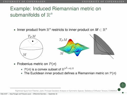
Example: Induced Riemannian metric onsubmanifolds of Rn
• Inner product from Rn restricts to inner product on M ⊂ Rn
• Frobenius metric on P(n)
• P(n) is a convex subset of R(n2+n)/2
• The Euclidean inner product defines a Riemannian metric on P(n)
Rightmost figure from Fletcher, Joshi, Principal Geodesic Analysis on Symmetric Spaces: Statistics of Diffusion Tensors, CVAMIA04
Slide 44/57 — Aasa Feragen and François Lauze — Differential Geometry — September 22
U N I V E R S I T Y O F C O P E N H A G E N U N I V E R S I T Y O F C O P E N H A G E N
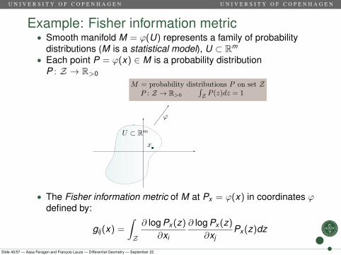
Example: Fisher information metric• Smooth manifold M = ϕ(U) represents a family of probability
distributions (M is a statistical model), U ⊂ Rm
• Each point P = ϕ(x) ∈ M is a probability distributionP : Z → R>0
• The Fisher information metric of M at Px = ϕ(x) in coordinates ϕdefined by:
gij (x) =
∫Z
∂ log Px (z)
∂xi
∂ log Px (z)
∂xjPx (z)dz
Slide 45/57 — Aasa Feragen and François Lauze — Differential Geometry — September 22
U N I V E R S I T Y O F C O P E N H A G E N U N I V E R S I T Y O F C O P E N H A G E N
Outline
1 MotivationNonlinearityRecall: Calculus in Rn
2 Differential GeometrySmooth manifoldsBuilding ManifoldsTangent SpaceVector fieldsDifferential of smooth map
3 Riemannian metricsIntroduction to Riemannian metricsRecall: Inner ProductsRiemannian metricsInvariance of the Fisher information metricA first take on the geodesic distance metricA first take on curvature
Slide 46/57 — Aasa Feragen and François Lauze — Differential Geometry — September 22
U N I V E R S I T Y O F C O P E N H A G E N U N I V E R S I T Y O F C O P E N H A G E N
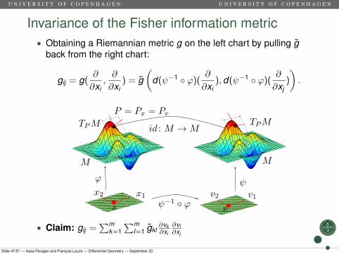
Invariance of the Fisher information metric• Obtaining a Riemannian metric g on the left chart by pulling g
back from the right chart:
gij = g(∂
∂xi,∂
∂xi) = g
(d(ψ−1 ◦ ϕ)(
∂
∂xi),d(ψ−1 ◦ ϕ)(
∂
∂xj)
).
• Claim: gij =∑m
k=1∑m
l=1 gkl∂vk∂xi
∂vl∂xj
Slide 47/57 — Aasa Feragen and François Lauze — Differential Geometry — September 22
U N I V E R S I T Y O F C O P E N H A G E N U N I V E R S I T Y O F C O P E N H A G E N
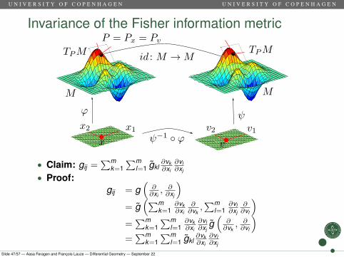
Invariance of the Fisher information metric
• Claim: gij =∑m
k=1∑m
l=1 gkl∂vk∂xi
∂vl∂xj
• Proof:gij = g
(∂∂xi, ∂∂xj
)= g
(∑mk=1
∂vk∂xi
∂∂vk,∑m
l=1∂vl∂xj
∂∂vl
)=∑m
k=1∑m
l=1∂vk∂xi
∂vl∂xj
g(
∂∂vk, ∂∂vl
)=∑m
k=1∑m
l=1 gkl∂vk∂xi
∂vl∂xj
Slide 47/57 — Aasa Feragen and François Lauze — Differential Geometry — September 22
U N I V E R S I T Y O F C O P E N H A G E N U N I V E R S I T Y O F C O P E N H A G E N
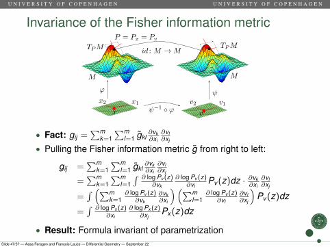
Invariance of the Fisher information metric
• Fact: gij =∑m
k=1∑m
l=1 gkl∂vk∂xi
∂vl∂xj
• Pulling the Fisher information metric g from right to left:
gij =∑m
k=1∑m
l=1 gkl∂vk∂xi
∂vl∂xj
=∑m
k=1∑m
l=1
∫ ∂ log Pv (z)∂vk
∂ log Pv (z)∂vl
Pv (z)dz · ∂vk∂xi
∂vl∂xj
=∫ (∑m
k=1∂ log Pv (z)
∂vk
∂vk∂xi
)(∑ml=1
∂ log Pv (z)∂vl
∂vl∂xj
)Pv (z)dz
=∫ ∂ log Px (z)
∂xi
∂ log Px (z)∂xj
Px (z)dz
• Result: Formula invariant of parametrizationSlide 47/57 — Aasa Feragen and François Lauze — Differential Geometry — September 22
U N I V E R S I T Y O F C O P E N H A G E N U N I V E R S I T Y O F C O P E N H A G E N
Outline
1 MotivationNonlinearityRecall: Calculus in Rn
2 Differential GeometrySmooth manifoldsBuilding ManifoldsTangent SpaceVector fieldsDifferential of smooth map
3 Riemannian metricsIntroduction to Riemannian metricsRecall: Inner ProductsRiemannian metricsInvariance of the Fisher information metricA first take on the geodesic distance metricA first take on curvature
Slide 48/57 — Aasa Feragen and François Lauze — Differential Geometry — September 22
U N I V E R S I T Y O F C O P E N H A G E N U N I V E R S I T Y O F C O P E N H A G E N
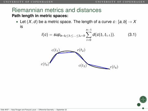
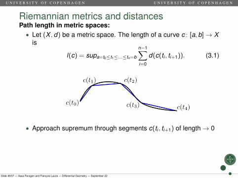
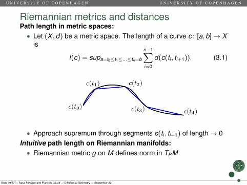
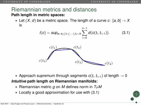
Riemannian metrics and distancesPath length in metric spaces:• Let (X ,d) be a metric space. The length of a curve c : [a,b]→ X
is
l(c) = supa=t0≤t1≤...≤tn=b
n−1∑i=0
d(c(ti , ti+1)). (3.1)
• Approach supremum through segments c(ti , ti+1) of length→ 0Intuitive path length on Riemannian manifolds:• Riemannian metric g on M defines norm in TPM• Locally a good approximation for use with (3.1)• This will be made precise in Francois’ lecture!
Slide 49/57 — Aasa Feragen and François Lauze — Differential Geometry — September 22
U N I V E R S I T Y O F C O P E N H A G E N U N I V E R S I T Y O F C O P E N H A G E N
Riemannian metrics and distancesPath length in metric spaces:• Let (X ,d) be a metric space. The length of a curve c : [a,b]→ X
is
l(c) = supa=t0≤t1≤...≤tn=b
n−1∑i=0
d(c(ti , ti+1)). (3.1)
• Approach supremum through segments c(ti , ti+1) of length→ 0
Intuitive path length on Riemannian manifolds:• Riemannian metric g on M defines norm in TPM• Locally a good approximation for use with (3.1)• This will be made precise in Francois’ lecture!
Slide 49/57 — Aasa Feragen and François Lauze — Differential Geometry — September 22
U N I V E R S I T Y O F C O P E N H A G E N U N I V E R S I T Y O F C O P E N H A G E N
Riemannian metrics and distancesPath length in metric spaces:• Let (X ,d) be a metric space. The length of a curve c : [a,b]→ X
is
l(c) = supa=t0≤t1≤...≤tn=b
n−1∑i=0
d(c(ti , ti+1)). (3.1)
• Approach supremum through segments c(ti , ti+1) of length→ 0Intuitive path length on Riemannian manifolds:• Riemannian metric g on M defines norm in TPM
• Locally a good approximation for use with (3.1)• This will be made precise in Francois’ lecture!
Slide 49/57 — Aasa Feragen and François Lauze — Differential Geometry — September 22
U N I V E R S I T Y O F C O P E N H A G E N U N I V E R S I T Y O F C O P E N H A G E N
Riemannian metrics and distancesPath length in metric spaces:• Let (X ,d) be a metric space. The length of a curve c : [a,b]→ X
is
l(c) = supa=t0≤t1≤...≤tn=b
n−1∑i=0
d(c(ti , ti+1)). (3.1)
• Approach supremum through segments c(ti , ti+1) of length→ 0Intuitive path length on Riemannian manifolds:• Riemannian metric g on M defines norm in TPM• Locally a good approximation for use with (3.1)
• This will be made precise in Francois’ lecture!
Slide 49/57 — Aasa Feragen and François Lauze — Differential Geometry — September 22
U N I V E R S I T Y O F C O P E N H A G E N U N I V E R S I T Y O F C O P E N H A G E N
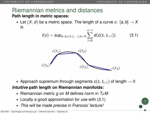
Riemannian metrics and distancesPath length in metric spaces:• Let (X ,d) be a metric space. The length of a curve c : [a,b]→ X
is
l(c) = supa=t0≤t1≤...≤tn=b
n−1∑i=0
d(c(ti , ti+1)). (3.1)
• Approach supremum through segments c(ti , ti+1) of length→ 0Intuitive path length on Riemannian manifolds:• Riemannian metric g on M defines norm in TPM• Locally a good approximation for use with (3.1)• This will be made precise in Francois’ lecture!
Slide 49/57 — Aasa Feragen and François Lauze — Differential Geometry — September 22
U N I V E R S I T Y O F C O P E N H A G E N U N I V E R S I T Y O F C O P E N H A G E N
Geodesics as length-minimizing curves
• We have a concept of path length l(c) for paths c : [a,b]→ M
• A geodesic from P to Q in M is a path c : [a,b]→ X such thatc(a) = P, c(b) = Q and l(c) = infcP→Q l(cP→Q).
• The distance function d(P,Q) = infcP→Q l(cP→Q) is a distancemetric on the Riemannian manifold (M,g).
Can you see why?
• Do geodesics always exist?
Slide 50/57 — Aasa Feragen and François Lauze — Differential Geometry — September 22
U N I V E R S I T Y O F C O P E N H A G E N U N I V E R S I T Y O F C O P E N H A G E N
Geodesics as length-minimizing curves
• We have a concept of path length l(c) for paths c : [a,b]→ M• A geodesic from P to Q in M is a path c : [a,b]→ X such that
c(a) = P, c(b) = Q and l(c) = infcP→Q l(cP→Q).
• The distance function d(P,Q) = infcP→Q l(cP→Q) is a distancemetric on the Riemannian manifold (M,g).
Can you see why?
• Do geodesics always exist?
Slide 50/57 — Aasa Feragen and François Lauze — Differential Geometry — September 22
U N I V E R S I T Y O F C O P E N H A G E N U N I V E R S I T Y O F C O P E N H A G E N
Geodesics as length-minimizing curves
• We have a concept of path length l(c) for paths c : [a,b]→ M• A geodesic from P to Q in M is a path c : [a,b]→ X such that
c(a) = P, c(b) = Q and l(c) = infcP→Q l(cP→Q).• The distance function d(P,Q) = infcP→Q l(cP→Q) is a distance
metric on the Riemannian manifold (M,g).
Can you see why?• Do geodesics always exist?
Slide 50/57 — Aasa Feragen and François Lauze — Differential Geometry — September 22
U N I V E R S I T Y O F C O P E N H A G E N U N I V E R S I T Y O F C O P E N H A G E N
Geodesics as length-minimizing curves
• We have a concept of path length l(c) for paths c : [a,b]→ M• A geodesic from P to Q in M is a path c : [a,b]→ X such that
c(a) = P, c(b) = Q and l(c) = infcP→Q l(cP→Q).• The distance function d(P,Q) = infcP→Q l(cP→Q) is a distance
metric on the Riemannian manifold (M,g). Can you see why?
• Do geodesics always exist?
Slide 50/57 — Aasa Feragen and François Lauze — Differential Geometry — September 22
U N I V E R S I T Y O F C O P E N H A G E N U N I V E R S I T Y O F C O P E N H A G E N
Geodesics as length-minimizing curves
• We have a concept of path length l(c) for paths c : [a,b]→ M• A geodesic from P to Q in M is a path c : [a,b]→ X such that
c(a) = P, c(b) = Q and l(c) = infcP→Q l(cP→Q).• The distance function d(P,Q) = infcP→Q l(cP→Q) is a distance
metric on the Riemannian manifold (M,g). Can you see why?• Do geodesics always exist?
Slide 50/57 — Aasa Feragen and François Lauze — Differential Geometry — September 22
U N I V E R S I T Y O F C O P E N H A G E N U N I V E R S I T Y O F C O P E N H A G E N
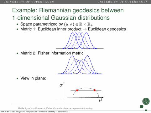
Example: Riemannian geodesics between1-dimensional Gaussian distributions• Space parametrized by (µ, σ) ∈ R× R+
• Metric 1: Euclidean inner product⇒ Euclidean geodesics
• Metric 2: Fisher information metric
• View in plane:
2
Middle figure from Costa et al, Fisher information distance: a geometrical reading
Slide 51/57 — Aasa Feragen and François Lauze — Differential Geometry — September 22
U N I V E R S I T Y O F C O P E N H A G E N U N I V E R S I T Y O F C O P E N H A G E N
Outline
1 MotivationNonlinearityRecall: Calculus in Rn
2 Differential GeometrySmooth manifoldsBuilding ManifoldsTangent SpaceVector fieldsDifferential of smooth map
3 Riemannian metricsIntroduction to Riemannian metricsRecall: Inner ProductsRiemannian metricsInvariance of the Fisher information metricA first take on the geodesic distance metricA first take on curvature
Slide 52/57 — Aasa Feragen and François Lauze — Differential Geometry — September 22
U N I V E R S I T Y O F C O P E N H A G E N U N I V E R S I T Y O F C O P E N H A G E N
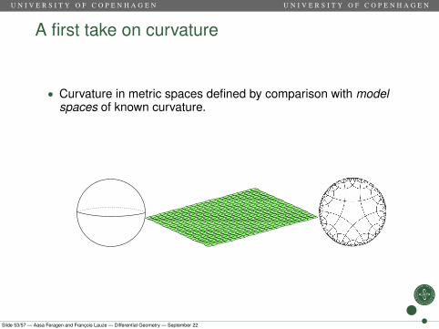
A first take on curvature
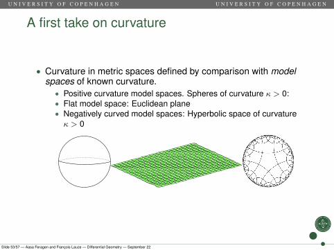
• Curvature in metric spaces defined by comparison with modelspaces of known curvature.
• Positive curvature model spaces. Spheres of curvature κ > 0:• Flat model space: Euclidean plane• Negatively curved model spaces: Hyperbolic space of curvatureκ > 0
Slide 53/57 — Aasa Feragen and François Lauze — Differential Geometry — September 22
U N I V E R S I T Y O F C O P E N H A G E N U N I V E R S I T Y O F C O P E N H A G E N
A first take on curvature
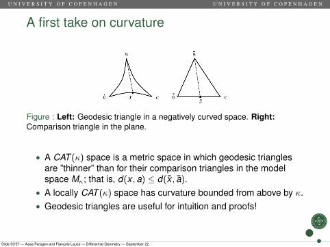
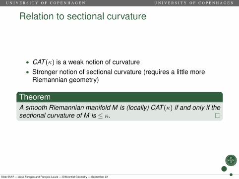
Figure : Left: Geodesic triangle in a negatively curved space. Right:Comparison triangle in the plane.
• A CAT (κ) space is a metric space in which geodesic trianglesare ”thinner” than for their comparison triangles in the modelspace Mκ; that is, d(x ,a) ≤ d(x , a).
• A locally CAT (κ) space has curvature bounded from above by κ.• Geodesic triangles are useful for intuition and proofs!
Slide 53/57 — Aasa Feragen and François Lauze — Differential Geometry — September 22

U N I V E R S I T Y O F C O P E N H A G E N U N I V E R S I T Y O F C O P E N H A G E N
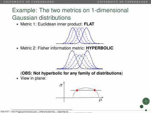
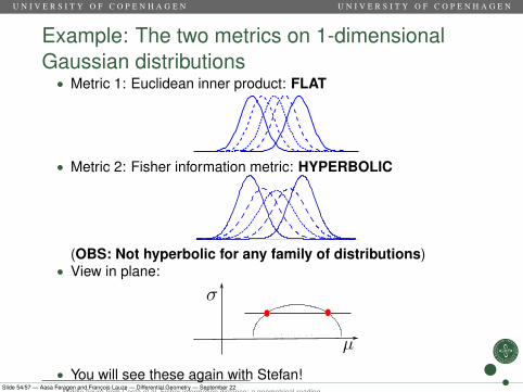
Example: The two metrics on 1-dimensionalGaussian distributions• Metric 1: Euclidean inner product: FLAT
• Metric 2: Fisher information metric: HYPERBOLIC
(OBS: Not hyperbolic for any family of distributions)• View in plane:
2
• You will see these again with Stefan!
Middle figure from Costa et al, Fisher information distance: a geometrical readingSlide 54/57 — Aasa Feragen and François Lauze — Differential Geometry — September 22
U N I V E R S I T Y O F C O P E N H A G E N U N I V E R S I T Y O F C O P E N H A G E N
Example: The two metrics on 1-dimensionalGaussian distributions• Metric 1: Euclidean inner product: FLAT
• Metric 2: Fisher information metric: HYPERBOLIC
(OBS: Not hyperbolic for any family of distributions)• View in plane:
2
• You will see these again with Stefan!Middle figure from Costa et al, Fisher information distance: a geometrical reading
Slide 54/57 — Aasa Feragen and François Lauze — Differential Geometry — September 22
U N I V E R S I T Y O F C O P E N H A G E N U N I V E R S I T Y O F C O P E N H A G E N
Relation to sectional curvature
• CAT (κ) is a weak notion of curvature• Stronger notion of sectional curvature (requires a little more
Riemannian geometry)
TheoremA smooth Riemannian manifold M is (locally) CAT (κ) if and only if thesectional curvature of M is ≤ κ.
Slide 55/57 — Aasa Feragen and François Lauze — Differential Geometry — September 22
U N I V E R S I T Y O F C O P E N H A G E N U N I V E R S I T Y O F C O P E N H A G E N
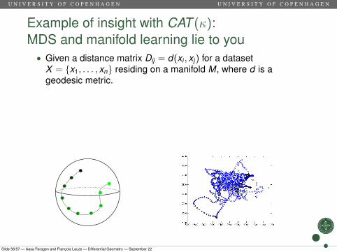
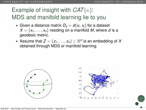
Example of insight with CAT (κ):MDS and manifold learning lie to you• Given a distance matrix Dij = d(xi , xj ) for a dataset
X = {x1, . . . , xn} residing on a manifold M, where d is ageodesic metric.
• Assume that Z = {z1, . . . , zn} ⊂ Rd is an embedding of Xobtained through MDS or manifold learning.
• Common belief: If d large, then Z is a good (perfect?)representation of X .
Slide 56/57 — Aasa Feragen and François Lauze — Differential Geometry — September 22
U N I V E R S I T Y O F C O P E N H A G E N U N I V E R S I T Y O F C O P E N H A G E N
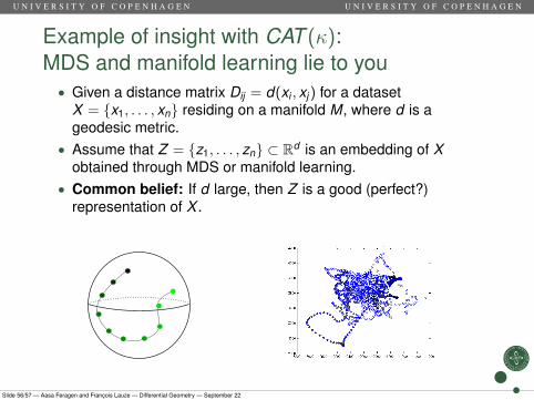
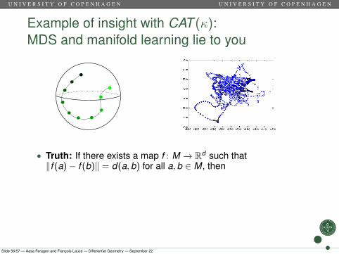
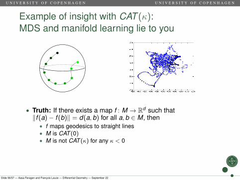
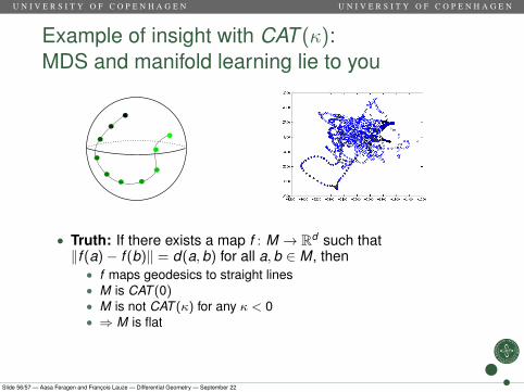
Example of insight with CAT (κ):MDS and manifold learning lie to you
• Truth: If there exists a map f : M → Rd such that‖f (a)− f (b)‖ = d(a,b) for all a,b ∈ M, then
• f maps geodesics to straight lines• M is CAT (0)• M is not CAT (κ) for any κ < 0• ⇒ M is flat
• That is, if M is not flat, MDS and manifold learning lie to you• (but sometimes lies are useful)
Slide 56/57 — Aasa Feragen and François Lauze — Differential Geometry — September 22
U N I V E R S I T Y O F C O P E N H A G E N U N I V E R S I T Y O F C O P E N H A G E N
Example of insight with CAT (κ):MDS and manifold learning lie to you
• Truth: If there exists a map f : M → Rd such that‖f (a)− f (b)‖ = d(a,b) for all a,b ∈ M, then
• f maps geodesics to straight lines• M is CAT (0)• M is not CAT (κ) for any κ < 0
• ⇒ M is flat• That is, if M is not flat, MDS and manifold learning lie to you• (but sometimes lies are useful)
Slide 56/57 — Aasa Feragen and François Lauze — Differential Geometry — September 22
U N I V E R S I T Y O F C O P E N H A G E N U N I V E R S I T Y O F C O P E N H A G E N
Example of insight with CAT (κ):MDS and manifold learning lie to you
• Truth: If there exists a map f : M → Rd such that‖f (a)− f (b)‖ = d(a,b) for all a,b ∈ M, then
• f maps geodesics to straight lines• M is CAT (0)• M is not CAT (κ) for any κ < 0• ⇒ M is flat
• That is, if M is not flat, MDS and manifold learning lie to you• (but sometimes lies are useful)
Slide 56/57 — Aasa Feragen and François Lauze — Differential Geometry — September 22
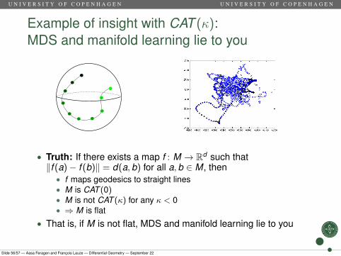
U N I V E R S I T Y O F C O P E N H A G E N U N I V E R S I T Y O F C O P E N H A G E N
Example of insight with CAT (κ):MDS and manifold learning lie to you
• Truth: If there exists a map f : M → Rd such that‖f (a)− f (b)‖ = d(a,b) for all a,b ∈ M, then
• f maps geodesics to straight lines• M is CAT (0)• M is not CAT (κ) for any κ < 0• ⇒ M is flat
• That is, if M is not flat, MDS and manifold learning lie to you
• (but sometimes lies are useful)
Slide 56/57 — Aasa Feragen and François Lauze — Differential Geometry — September 22
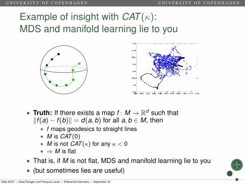
U N I V E R S I T Y O F C O P E N H A G E N U N I V E R S I T Y O F C O P E N H A G E N
Example of insight with CAT (κ):MDS and manifold learning lie to you
• Truth: If there exists a map f : M → Rd such that‖f (a)− f (b)‖ = d(a,b) for all a,b ∈ M, then
• f maps geodesics to straight lines• M is CAT (0)• M is not CAT (κ) for any κ < 0• ⇒ M is flat
• That is, if M is not flat, MDS and manifold learning lie to you• (but sometimes lies are useful)
Slide 56/57 — Aasa Feragen and François Lauze — Differential Geometry — September 22

U N I V E R S I T Y O F C O P E N H A G E N U N I V E R S I T Y O F C O P E N H A G E N
A message from Stefan for tomorrow’s practical
Check out course webpage for installation instructions!http://image.diku.dk/MLLab/IG4.php
Slide 57/57 — Aasa Feragen and François Lauze — Differential Geometry — September 22