u-ivi·i - scholarspace.manoa.hawaii.edu · a sample of 614 households from ... model specification...
TRANSCRIPT

INFORMATION TO USERS
This manuscript has been reproduced from the microfilm master. UMI
films the text directly from the original or copysubmitted. Thus, some
thesis and dissertation copies are in typewriter face, while others may
be from any type of computer printer.
The quality of this reproduction is dependent upon the quality of thecopy submitted. Broken or indistinct print, colored or poor quality
illustrations and photographs, print bleedthrough, substandard margins,
and improper alignment can adverselyaffect reproduction.
In the unlikely event that the author did not send UMI a complete
manuscript and there are missing pages, these will be noted. Also, if
unauthorized copyright material had to be removed, a note will indicate
the deletion.
Oversize materials (e.g., maps, drawings, charts) are reproduced by
sectioning the original, beginning at the upper left-hand corner and
continuing from left to right in equal sectionswith small overlaps. Each
original is also photographed in one exposure and is included in
reduced form at the back of the book.
Photographs included in the original manuscript have been reproducedxerographically in this copy. Higher quality 6" x 9" black and white
photographic prints are available for any photographs or illustrations
appearing in this copy for an additional charge. Contact UMI directly
to order.
U-IVi·IUniversity Microfilms International
A Bell & Howell Information Company300 North Zeeb Road. Ann Arbor. M148106·1346 USA
3131761·4700 800/521-0600


Order Number 9129681
Life-cycle analysis of household composition and familyconsumption behavior
Kanel, Nav Raj, Ph.D.
University of Hawaii, 1991
u rvl·I300 N. Zeeb Rd.Ann Arbor, MI 48106


LIFE-CYCLE ANALYSISOF
HOUSEHOLD COMPOSITIONAND
FAMll,y CONSUMPTiON BEHAVIOR
A DISSERTATION SUBMITTED TO THE GRADUATE DIVISION OF THEUNIVERSITY OF HAWAII IN PARTIAL FULFILLMENT OF THE
REQUIREMENTS FOR THE DEGREE OF
DOCTOR OF PHILOSOPHY
IN ECONOMICS
MAY 1991
By
Nav Raj Kanel
Dissertation Committee:
Andrew Mason, ChairmanBurnham Campbe!l
John BauerCalla Wiemer
James Palmore, Jr.
©Copyright by Nav Raj Kanel1991
All Rights Reserved
iii

To
my mother
in appreciation of her love and affection
and
my brother Tej
in appreciation of his support and encouragement
that I pursue my education, which led finally to this dissertation
iv

ACKNOWLEDGMENTS
This work has deepened and broadened my debts to all those who offered their
cooperation, help, and constructive suggestions for the successful completion of
this project. Although not all can be mentioned, certainly all are thanked for
their contributions. However, I would like to thank the following persons and
institutions for making this research possible:
• The East-West Population Institute deserves the first mention for providing
generous financial support throughout my study and field research
• Prof. Andrew Mason, my advisor and committee chair, for his advice, time,
and guidance in helping me improve this dissertation, as well as fer his
continued encouragement and reassurance during the various stages of com
pleting my degree
• Other members of my dissertation committee, Profs .. James Palmore, Burn
ham Campbell, John Bauer, and Calla Wiemer, each of whom contributed
significant personal strengths and insight; and Profs. Robert Retherford
and Fred Arnold of the East-West Population Institute for their invaluable
suggestions regarding my questionnaire
e Profs. Harold Rowe, and Hessel Flitter for their continuous support, en
couragement, and care during my whole study period in Honolulu
o Prof. Parthibeshwor Timilsina, for supervising my field study in Nepal;
Messrs. Ram Pokharel, Madhav Bhardwaj, and Bishnu Rijal for their data
enumeration assistance; and Mr. Ashoke Shrestha for letting me use New
ERA's computers to enter my field data
v

• All the respondents of my household survey for their patience, time, and
cooperation in sincerely answering my questions without which this project
would not have been successful
• Tribhuvan University (Nepal) for approving my leave from the university
during the period of my study
• Ms. Gayle Yamashita, Dr. Rachel Racelis, and Dr. David Ho for patiently
answering my computer questions
• Ms. Anne Stewart for reviewing this dissertation
o My mother and my brothers Tej, Bhesh, and Keshav for their love, in
spiration, moral support, and confidence in me that I could successfully
accomplish my goal
• And finally, my wife Dev, my son Pawan, and my daughter Moana for their
endless patience and every support throughout this project
To those mentioned, as well as to many others who were not, who helped to make
this study not only possible but enjoyable, I extend my heartfelt dhanyabad,
mahalo, and thanks. However, I have no excuses for errors and I alone am
responsible for any remaining errors and discrepancies.
vi

ABSTRACT
The purpose of this study is to assess the demographic impact of household
composition on the consumption behavior of Nepali households over the family
life-cycle, employing consumer demand theory. Household size and household
composition are distinguished, and particular attention is focused on changing
household composition and life-cycle consumption. Other factors examined are
future household composition, demographic scaling, effects of different lifetime
discount rates, and bequest motives.
The life-cycle model of consumer demand theory originally advanced by
Modigliani and Brumberg (1954) is employed and extended to investigate how
changing household size and composition over the family life-cycle affects the
consumption behavior of selected households. A sample of 614 households from
Kathmandu Valley was taken during the winter of 1987-88 to represent the
demographic structure and income-expenditure patterns of Nepali households.
This study shows the life-cycle consumption of Kathmandu households in
a changing household composition pattern. HOMES, A Household Model for
Economic and Social Studies, is applied to project a family of curves of fu
ture household membership. This information is used to estimate the life-cycle
consumption function that explicitly incorporates expected lifetime household
membership. Equivalence scales are estimated to measure the effect of house
hold age-sex composition on consumption.
The findings confirm the importance of demographic variables in household
consumption. The equivalent adult units that provide an alternative measure
of the net effect on consumption of a specific household member are estimated.
The estimated equivalent adult units for children, teenagers, and adult females
vii

are respectively 0.94, 1.46, and 0.92, assuming that the equivalent adult unit of
all adult male is one. These large values of the equivalent units suggest that
children have a stronger effect in Nepal than typically found in the literature.
The demographic variables are jointly, but not individually, significant. This
study is limited by a small sample size. Therefore, no firm conclusions could be
drawn.
Two factors may account for the teenage coefficients. First, teenagers do
not contribute to the household income. Second, education in Kathmandu, par
ticularly up to high school, is very expensive. Heavy outlays for tuition, fees, and
school supplies wake teenagers more expensive to support than other members.
Yet, the value of 1.46 cannot be distinguished from unity.
Testing our model's general specification to examine the validity of the model
and variables therein suggests that the relationship between demographic vari
ables and consumption is not as simple as specified by the model. The equivalent
adult unit for teenagers is also significantly different from one. This model also
rejected the hypothesis that the bequest parameter is equal to zero. This con
firms that the bequest motive is important and should be incorporated in the
life-cycle model.
The model developed here provides a better way for assessing the impact of
current demographic characteristics on current needs relative to lifetime needs.
The effect of demographic variables i'.4 "''llly through the existing age-sex
composition of the household but also throug l,e expected lifetime composi
tion. The findings suggest that household comp, . '1n has an important role
in determining household consumption ratio, which 'urn affects saving and
economic development.
viii

TABLE OF CONTENTS
ACKNOWLEDGMENTS
ABSTRACT ...
LIST OF TABLES
LIST OF FIGURES
CHAPTER 1. INTRODUCTION
1.1 Statement of the Research Problem
1.2 Objectives and Methodology
1.3 Outline of the Study . . . . . . .
CHAPTER 2. REVIEW OF THE LITERATURE
v
vu
xu
Xlii
1
1
3
5
6
2.1 Life-Cycle Analysis of Consumption: A Forward-Looking Theory 7
2.2 Further Development and Applications of the Life-Cycle Model 9
2.2.1 Development of the Model 9
2.2.2 The Bequest Issue: An Unreconciled Debate 15
2.2.3 On Saving and Population Growth . . . . 20
2.3 Demographic Variables in Consumption Analysis 23
2.4 Other Socioeconomic Studies . . . . . . . 28
CHAPTER 3. THEORETICAL CONSTRUCT AND
MODEL SPECIFICATION 30
3.1 Theoretical Construct . . 30
3.1.1 The Utility Function . 32
3.1.2 The Budget Constraint 33
3.2 Model Specification 36
3.2.1 Theoretical Model . 36
3.2.2 Econometric Model 40
ix

CHAPTER 4. HOUSEHOLD SURVEY . . . . . . . . . . 43
4.1 Location, and Method of Data Collection
4.2 Household Characteristics .
4.2.1 Household Types . . . . . .
4.2.2 Ethnicity and Mother Tongue of Heads
4.2.3 Educational Attainment of Heads
4.2.4 Occupation of Heads . . . . . . . .
4.3 Household Income, Expenditures, and Net Assets
4.3.1 Household Income . . .
4.3.2 Household Expenditures
4.3.3 Household Net Assets
4.4 Inheritances and Bequests
4.4.1 Inheritances
4.4.2 Bequests
44
49
49
54
55
57
58
60
60
62
64
65
66
CHAPTER 5. PROJECTING FUTURE HOUSEHOLD COMPOSITION 69
5.1 Structure of Nepali Households . . . . . . . . . . . 69
5.2 The Household Life-Cycle 72
5.3 Projecting the Expected Number of Household Members 74
5.3.1 Calculating Membership Profiles for Individual Households 77
5.3.2 Calculating Household Survival Ratios . . . . . . . ., 80
CHAPTER 6. ESTIMATION AND EMPIRICAL FINDINGS . . . . . 83
6.1 Estimation Procedure
6.2 Statistical Tests . . .
6.2.1 Testing Hypotheses
6.2.2 Testing the Model's Specification
6.3 Estimated Functions and Discussion
6.4 Summary .
x
86
89
89
90
91
101
CHAPTER 7. CONCLUSIONS AND POLICY IMPLICATIONS 102
7.1
7.27.3
Major Results and Policy Implications . . . . . . . .
Limitations of the Study and Suggestions for Future Research
Conclusions
102
105
107
APPENDIX . . . . . . . . . . . . . . . . . . . . . . . . . . . 109
REFERENCES 121
xi
2.1
4.1
4.2
4.3
4.4
4.5
4.6
4.74.8
4.9
4.10
4.11
4.12
4.13
4.14
4.15
5.1
5.2
5.3
6.1
6.2
6.3
6.4
LIST OF TABLES
Demographic Variables in Demand Equations
Distribution of Households in Kathmandu.
Age Dlstributlon of Household Heads
Distribution of Household Types
Distribution of Household Size
Marital Status of Household Heads
Average Number of Household Members
Ethnicity and Mother Tongue of Households
Educational Attainment of Heads and Members
Occupation of Household Heads . .
Income Distribution of Households
Distribution of Annual Expenditures
Household Net Assets ....
Average Income, Expenditures, and Assets
Inheritance by Household Heads ..
Intended Bequests of Household Heads .
Members by Relationship in Family Households
Age-Specific Fertility Rates . . . . . . .
Household Survival Ratios .
Mean Values of Demographic and Economic Variables
Parameter Estimates for Different Models ..
Testing the Effect of Age and Sex on Consumption
Testing the Model Specification . .. ...
xii
26
4748
50
51
52
53
55
56
58
61
62
63
65
66
67
70
7781
85
92
95
98

5.1
5.2
6.1
LIST OF FIGURES
Intact Households
Average Members per Household
Life-Cycle Equivalent Adults
xiii
73
78100
CHAPTER 1
INTRODUCTION
1.1 Statement of the Research Problem
The microeconomic theory of consumer behavior tells us that the consumption
combinations of an individual depend upon the tastes and income of the consumer
and the relative prices of all commodities that he faces. This theory is based on
the assumption that a rational consumer will always try to maximize his utility
function subject to a budget constraint. But when we take a household as a
consumer unit, consumption depends not only on those variables, but also on
the composition of the household.
In economics, the terms "household" and "family" have often been used
synonymously because of their close relationship. By definition, a "household"
corresponds to the living arrangements of its members, whereas a "family" cor-
responds to the relationship among the household members. 1 Household compo-
sition is described by the number of members and the age-sex structure of the
household. As the composition of a household changes, the tastes and necessi
ties of the household will also change. Consequently, a change will occur in the
demand for commodities. However, when we take a family as a consumer unit,
consumption depends not only on those variables, but also on the life-cycle of
the family.
1 Pressat (1985), and Howard (1971) and references therein have a more detailed discussionon the definitions and concepts of household and family.
1
The family life-cycle is an idealized construct representing the important
stages in the life of an ordinary family. Births, deaths, marriages, changes in
the age-sex structure of the family, and the formation of a new household will
elicit different turning points in the family regarding its consumption patterns.
Such turning points in a family will introduce new stages in the family life-cycle.
Although the concept of the life-cycle is clearly related to the process of aging,
the concept derives its analytical utility from the social and economic significance
of the events and stages that mark the life-cycle.
Demographically, as well as economically, Nepal is typical of many less de
veloped countries with its low per capita income, high total fertility rate, high
birth rate, high death rate, high infant mortality rate, and low life expectancy
(Kanel, 1986). A very large proportion of Nepali households is family households.
Therefore, the concepts of household and family can be regarded as synonyms in
the context of Nepal.
The traditional as well as the modern form of family in Nepal, both rural
and urban, is the extended family consisting of three (or even more) generations.
The extended family system is part of the culture and tradition of Nepali society.
Higher co-residence rates, i.e., the proportion of the elderly over 65 who reside
with their children and/or other relatives, is mainly due to the traditional values
accorded to the family and household in Nepal. Older parents also do some
household work such as cooking, baby-sitting, and household management. This
does not mean, however, that there are no nuclear families in Nepal. Economic
scarcity in such societies requires that all members of the family be engaged in
the productive activities of the household.
2

Economists have agreed that the life-cycle of a family (or a household) is
an important determinant of household consumption patterns. Modigliani and
Brumberg (1954) originally advanced the life-cycle hypothesis of consumption
theory. This theory assumes that households (or individuals) have a finite life
span and that they strive to maximize their utility from current and future
consumption subject to current resources and their expected future income. Ac
cording to this hypothesis, the planned consumption path reflects the allocation
of lifetime resources to consumption over the life span. It emphasizes the process
of saving during working years for consumption during retirement. The life-cycle
model provides a crucial link between the microeconomics of rational household
behavior and the macroeconomics of the rate of saving.
This model was later further developed and modified by many economists
such as Fisher (1956), and Modigliani and Ando (1957). They applied this theory
to analyzing the case of different countries which have a nuclear family system.
Some of its applications and extensions will be discussed in Chapter 2 (Review
of the Literature). However, no attempts appear to have been made so far to
apply this theory to the case of an extended family system. This study seeks
to extend this model to examine the consumption behavior of extended families
by incorporating inheritances and bequests into the objective function and the
budget constraint of the household.
1.2 Objectives and Methodology
The objective of this study is to examine the effect of changing household size and
composition on the consumption patterns of Nepali households over the family
life-cycle, employing consumer demand theory. Consumption behavior in such
3

systems is explained by demographic variables and by a household bequest mo
tive. This theory is based on the postulate that a household tries to maximize
its welfare by adjusting consumption expenditures as it moves through different
life-cycle stages. Household size and household composition are distinguished,
and particular attention is focused on changing household composition and life
cycle consumption. Other factors examined are future household composition,
demographic scaling, effects of different lifetime discount rates, and bequest mo
tives.
The life-cycle model of consumer demand theory originally advanced by
Modigliani and Brumberg (1954) is employed and extended to investigate how
changing household demographics over the family life-cycle affects the consump
tion behavior of selected households. The effect of demographic variables is not
only through the existing age-sex composition of the household but also through
the expected lifetime composition. A nonlinear consumption function, where
consumption is a function of current and expected lifetime household composi
tion, bequest motive, household income and assets, and life expectancy of the
household head, is derived. An alternative specification is also examined to test
the validity of the general model and variables therein.
HOMES, Household Model for Economic and Social Studies, is applied to
project a family of curves of future household membership. This information is
used to estimate the life-cycle consumption function that explicitly incorporates
expected lifetime household membership. Nonlinear regression equations are es
timated using maximum likelihood method. Equivalence scales are estimated to
measure the effect of household age-sex composition on consumption. The anal
ysis and the inferences drawn therefrom are based on a sample of 614 households
4

taken from Kathmandu Valley during the winter of 1987-88 to represent the
demographic structure and income-expenditure patterns of Nepali households.
1.3 Outline of the Study
This dissertation is divided into seven chapters. Chapter 2 reviews the relevant
literature on life-cycle analysis and the incorporation of demographic variables
into consumption theory. Chapter 3 is devoted to examining the theoretical
framework and model specification for the present study. In Chapter 4, I will
discuss the data. Projection of future household composition is described in
Chapter 5. In Chapter 6 estimated consumption functions and their interpre
tations are reported. Statistical tests of the model and their analyses are also
presented in that chapter. And finally, a summary of findings, the policy impli
cations of the study, and suggestions for further research are included in Chapter
7.
5

CHAPTER 2
REVIEW OF THE LITERATURE
Eizenga's (1961) analysis of the 1950 U.S. Survey of Consumer Expenditures is
one of the first attempts to examine the relationship between household size and
household consumption. His findings show that the absolute level of standardized
household savings declines as household size increases. Controlling for household
income and age and occupation of head, Eizenga finds that saving declines very
substantially as family size increases from one to three members, but declines
much more gradually thereafter. Similarly, David (1962) found that the size of
the family or the age of the household head is more important in determining
expenditures on housing, whereas marital status appears to be a more important
factor in consumption of automobiles.
Barten (1964) was the first economist to introduce and discuss demand func
tions incorporating household size and composition into the model. He intro
duced a set of parameters, known as "specific equivalent adults," to measure the
size and composition of a household. Muellbauer (1974), and Bojer (1977) have
further explored Barten functions, both theoretically and empirically, to exam
ine the effects of household composition on household demand. None of these
studies were based on life-cycle models. We shall, however, confine our literature
survey to the discussion of studies that utilized the theoretical construct of the
life-cycle hypothesis and procedures for incorporating demographic variables into
household utility functions.
Analysis of demographic variables in the life-cycle model has received con
siderable attention because the costs of rearing children have significant effects on
6

the allocation of household's resources over its lifetime. Both direct costs, such
as the increase in household expenditures, and the indirect costs of rearing chil
dren have been examined intensively. Direct costs have been estimated by many
researchers (for example, Pollak and Wales, 1978, 1981; Olson, 1983; Deaton and
Muellabauer, 1986). The estimates and findings show that expenditures on chil
dren definitely increase with the number and age of children. Devaney (1984),
examining indirect costs, concludes that the presence of children in a house
hold has a pronounced negative influence on female labor force participation and
consequently on household income.
2.1 Life-cycle Analysis of Consumption: A Forward-Looking Theory
A number of different theories of consumption have been developed in response
to the myopic nature of the simple consumption function.
One of these is the life-cycle hypothesis of consumption theory, which has
been widely tested, applied, and developed. This theory derives its name from
its emphasis on an individual (or family) looking ahead over its entire lifetime.
The life-cycle model is an attempt to examine the magnitude and implications
of transitory saving and hump wealth by relating it to the classical theory of
consumer choice and more particularly to the hypothesis of optimal allocation of
time. We can also refer to it as a forward-looking theory of consumption because
this theory embodies the basic idea that individual consumers are forward-looking
decision makers. This theory is the microfoundation of macroeconomics and
offers a simple story of a representative consumer or household. It provides a
crucial link between the microeconomics of rational household behavior and the
macroeconomics or the rate or saving.
7

The life-cycle model originally advanced, developed, and popularized by
Modigliani and his associates (Modigliani and Brumberg, 1954; Modigliani and
Ando, 1957; Ando and Modigliani, 1963) emphasizes the importance of sav
ing during periods of relatively high earnings for consumption during periods
of relatively low earnings. Therefore, this theory breaks rank with the simple
consumption function by saying that consumers do not concentrate exclusively
on a single year's disposable income. Instead, they also look ahead to their likely
future incomes, which will depend on their future earnings, wealth, and the tax
structure.
According to the Modigliani and Brumberg (1954) model, the consumption
function can simply be expressed as
c: = "'Jtv:T IT T (2.1)
where C;' is the household consumption in period r as anticipated from period
t, 'Y~ is the proportion of total household resources consumed in period". as
anticipated from period t (depending upon the utility function and the rate of
interest but not on Vt ) , Vt is the size of expected total (discounted) lifetime
household resources as anticipated from the planning period t, and L is the final
period of the household's life.
H there is no bequest or inheritance, and the real rate of interest is zero,
then
(2.2)
Or, all resources will be consumed during the total life span.
8
If we further assume that consumption is constant in each period, i.e., 1~ =
" then from (2.2) we have (L + 1- r)-y = 1. Therefore,
(2.3)1
T.JUT
11=1~= (L+1-1") =-
where L T = (L +1- r) denotes the remaining life span at time r, This shows
that the fraction of lifetime resources consumed in each period is equal to the
inverse of the life span.
Equation (2.3) shows that 1;, the proportion of total resources consumed in
period r, depends on the age of the consumer, not on the income level. This is
the unique feature of the life-cycle model.
This hypothesis shares some traits with the permanent income hypothesis
(Friedman, 1957) which shows that the marginal propensity to consume out of
transitory income is zero. In both models, the marginal propensity to consume
is independent of lifetime income. Friedman (1957) assumed, as Modigliani and
Brumberg (1954) did, that households strive to maximize their utility of future
consumption. The decisive difference between the two theories concerns the
length of the planning period. In the Modigliani-Brumberg version, the planning
period is finite, i.e., people save only for themselves. According to Friedman,
however, this period is infinite.
2.2 Further Development and Applications of the Life-cycle Model
2.2.1 Development of the Model
Modigliani and Brumberg's work (1954) is the cornerstone of the life-cycle hy-
pothesis of consumption theory. This hypothesis assumes that households (or
9

individuals) strive to maximize their utility from current and future consump
tion subject to their expected total income, that is, the sum of current income
and assets and discounted future earnings. Based upon this hypothesis, four
successive models have been developed as its extension in order to examine the
relationship between household consumption and demographic variables.
The original formulation by Modigliani and Brumberg (1954) was aimed at
analyzing the case of an individual. Their theory assumes that individuals (or
households) strive to maximize their utility from current and future consump
tion subject to their expected future income. Fisher (1956) introduced family
size into the life cycle model. Both Tobin's (1967) simulation model and Leff's
(1969) econometric approach have employed the life-cycle framework for model-
ing the relationship between saving and demographic factors.' Other empirical
studies such as Ando and Modigliani (1963), using aggregate time-series data,
and Modigliani (1970), using cross-country data, demonstrate the usefulness of
this model.
This theory can be applied to stationary economies, as well as to growing
economies, and we can also allow for different assumptions. Accordingly, several
recent extensions and applications of this model, namely the introduction of so-
cial security by Feldstein (1976), Evans (1982), and David and Menchik (1985);
incorporation of initial assets and intended bequests by Blinder (1976), Mariger
(1983), and David and Menchik (1985); determination of the role of bequests
iT'. the process of wealth accumulation by White (1978), Kotlikoff and Summers
1 Because the saving ratio equals one minus the consumption ratio, factors that increase theconsumption ratio, by definition, decrease the saving ratio by an equal amount. Therefore,these two ratios are complement to each other.
10

(1981), Ev<.l.Ils (19~.2, 1984), Kotlikoff (1988), and Modigliani (1988); examina
tion of the effect of uncertainty on saving behavior by Short (1986); investigation
of the effect of government expenditures and taxes on private consumption by
Modigliani and Sterling (1986); and a study on the effect of household compo
sition on the consumption behavior of chicken farm households in Thailand by
Arphasil (1988), have proved the applicability of the life-cycle hypothesis. A
number of studies have also rejected the "textbook" version definition of the life
cycle hypothesis-that the elderly dissave out of accumulated wealth to finance
the continuation of preretirement consumption levels after retirement.
The original Modigliani-Brumberg model treated households as though they
were individual consumers. They did not, however, include family size in their
model. Fisher (1956) was the first to call attention to the absence of families
in the life-cycle model and to do an empirical study introducing family size. To
capture the effect of variations in household size on 'Y~, Fisher disaggregated it
into two parts: 'YTl which is independent of family size, and bTl which measures
the effect of household size. Therefore, 'Y; can be rewritten as
(2.4)
where J: is the expected family size in period T.
Modigliani and Ando (1957) later refined the Modigliani-Brumberg model
as well as the empirical work of Fisher. They modified the model to measure the
effect of the age of members as well as their numbers. H we assume that adults
consume more than children, a household with older children, ceteris paribus,
should consume more than a household with younger children. Redefining b; as
bT = aTgn and with some rearrangement of terms, they derived the relationship
11

CT
= Vt[l + aT(mJ: - 1)]L T[I + aT(mJ: - 1)] (2.5)
where mJ;(= E~=t J:ILT) is the weighted mean of the numbers in the family in
each time period, the weight is the number of periods in which J members are in
the family, aT measures the effect of age and household size, and LT= (L +1- r]
is the remaining period of life."
Equation (2.5) shows that consumption depends on the size of the house
hold, as well as its life span. Therefore, it provides us with the basic function to
estimate the effect of household size in the life-cycle model. However, this model
does not answer all other questions that remain to be answered. It does not allow
for the effect of the age of children on household consumption and economies of
scale in childrearing. The works of Fisher and Modigliani-Ando provide an eval
uation of the life-cycle hypothesis when allowing for variations in household size
but they fail to determine the effect of household size on household consumption.
A different approach to analyzing the size and savings behavior of households
was undertaken by Somermeyer and Bannink (1973). Those authors applied the
life-cycle saving model directly by estimating lifetime household resources. They
defined the ratio of current consumption to estimated lifetime resources as a
measure of the household's "urgency to consume." Using the same notations as
Fisher, the "urgency to consume" can be simply defined as
(2.6)
Somermeyer and Bannink (1973) estimate the value of lifetime resources as
2 The full derivation of (2.5) from (2.4) is given in Modigliani and Ando (1957: 111-112).
12

where At is the value of assets held at the beginning of period t, yt is the value of
all household labor income if held to period L, K t is the value of capital income
earned from At if held to period L, and L 1' = (L -.,. +1) is the remaining length
of life.
The authors state that if the earnings rate on A! is less than the interest
rate (r), then the household will consume out of At at a price below that asserted
in the model. If, however, the return to At exceeds r and the household's con
sumption in period t exceeds the income earnings Yt + K t , the household must
be consuming out of At and at a price that is above that assumed in the model.
Estimations of the interest rate, Yt for individual members of the household, and
variations in future income from changes in the composition of the household
are some of the additional problems with this approach. They take the Nether
lands as their case study. With an interest rate equal to 4.08 percent throughout
the analysis, their results show that the mean values of "YtLt range from 1.50 to
1.97. If the childless households plan to consume equal amounts in each period,
"YtLt should be less than one, because r is positive and Vt is the value of lifetime
resources,"
Mason (1975) extended the model derived by Fisher (1956), and Modigliani
and Ando (1957). His analysis is confined to the effect of household size on
the fraction of household resources consumed over the entire childrearing period.
Equation (2.4) is modified to circumvent the problem of the effect of age of chil
dren on household consumption. Therefore, he separates life-cycle consumption
3 This paragraph draws heavily from Mason (1975: 27-30).
13
into two successive periods: the childrearing period and the post childrearing
period. He disaggregated the coefficient of the consumption function as
a*
'1; = 'Yr[l+ b1 +~ b2(a)Jr(a)]~
a=O(2.7)
where a* is the (average) age at departure from the household by children, and
Jr(a) is the number of children at time T of age a. Substituting equation (2.7)
into equation (2.1) and rearranging the terms, it will yield to
(Va - V~) _ RVo = (b2 ) JVO VO bo m
n n(2.8)
where V~ = (1 + r) -nvn,R = E~;OI(l + r)-t / E;=o(1 + r)-t,
bo = (1+b1) 2:;=0(1 +r)-t, mJ is the discounted number of children ever born,
and n is some time period, t = n, for which Jt(a) = 0 for t greater than or equal
to T, i.e., T is greater than (tj + a*).4
The right side of equation (2.8) is the consumption demands on initial life
time household resources of children relative to adults. b2/bo measures the effect
of household size on relative consumption, where bo is the discounted fraction
of total resources consumed by parents. Therefore the ratio of b2 to bo can also
be thought of as the relative equivalent adult scales of children's consumption.
The left hand side expression represents the proportion of total lifetime resources
devoted to consumption. The first term on the left hand side is the initial value
of lifetime resources devoted to consumption between periods 0 and n -1 relative
to resources devoted to consumption after period n - 1. The second term is the
proportion of initial lifetime resources devoted to (0, n -1) consumption relative
4 For further detail flee Mason (1975: 42-49).
14

to (n,L) consumption were consumption evenly spread over the household's life.
The sensitivity test of consumption using different rates of interest showed that
household size has a small effect on consumption when the rate of interest is
high; the constant term will be negative implying the over-estimation of the rel
ative effect of child-consumption; and the higher absolute value of the constant
term indicates that other important factors combined strongly affect household
consumption rather than mere the number of children.
It is observed from the preceding studies that economists have analyzed the
relationship between household size and life cycle consumption for a household
as initiated by Fisher (1956). They have also reflected the effect of household
size on consumption through 'Y~, the coefficient of the lifetime resources in the
consumption function.
2.2.2 The Bequest Issue: An Unreconciled Debate
Although the life-cycle theory remains the leading microeconomic theory of con
sumption behavior, the assumption that there are no planned bequests is one
of the most controversial assumptions underlying this model. The assumption
that people save mainly for retirement and dissave out of accumulated wealth
to finance their retirement has also been questioned by recent findings. These
studies argue that people's actual planning horizon is longer than their full life
time. According to this view, people intentionally leave bequests or make gifts,
signifying that they derive satisfaction from the economic well being of future
generations and have a multigenerational planning horizon [Barro, 1974; Becker,
1974; Kotlikoff and Summers, 1981; Hayashi, 1986; Kotlikoff, 1988).
15

Blinder (1976) included capital market constraints and bequests in the orig
inal life-cycle model. He concluded that, under uncertainty, the life-cycle hy
pothesis that the lifetime pattern of consumption is independent of the lifetime
pattern of earnings is not true. Blinder et al. (1983) have incorporated the be
quest motive, proxied by the number of children, to study the asset holdings of
white American men near retirement age. Their results show that the life-cycle
model has little ability to explain cross-sectional variability in asset holdings.
Darby (1979) inferred longitudinal age-consumption and age-earnings profiles
from the cross section profile and concluded that not more than 29 percent of
U.S. private net worth is devoted to future consumption with the rest destined for
intergenerational transfer. White (1978) used aggregate data on the age struc
ture of the population, age earnings, and age consumption profiles along with
a variety of parametric assumptions and she concludes that the life-cycle model
can account for only about one-quarter of aggregate saving.
Some recent findings question the assumed motive for saving and the im
plication that people dissave their wealth when old. Friedman's (1957) theory
of consumption, which is contemporary to the life-cycle theory, assumes infinite
time horizon which could imply that people save not only for themselves but also
for their descendants. Kotlikoff and Summers (1981) have shown that most sav
ing is done to provide bequests rather than to provide for old-age consumption.
Kotlikoff (1988) argues that there is strong evidence that intergenerational trans
fers playa very important and perhaps dominant role in wealth accumulation in
the United States. He further asserts that altruistic concern for one's children is
the first reason one thinks of for intergenerational transfers. This concern may
be expressed mathematically as the parent having direct utility for the utility of
16

the child as in Barro (1974) and Becker (1974). They conclude that though the
savings are for the consumption in retirement, people are saving mainly to pass
wealth on to their descendants.
Modigliani (1986), however, takes issue with the calculations that underlie
the Kotlikoff-Summers (1981) claim that most savings are for bequests. Kotlikoff
and Summers (1986) subsequently identified an error in the treatment of durable
goods. They indicated that a proper correction for durables raises the share of
wealth accumulation in life-cycle saving to 21.9 percent from 18.9 percent they
had reported in their 1981 paper.
Another study done by Danziger et al. (1982-83) shows that there is
strong evidence contradicting the "textbook" version definition of the life-cycle
hypothesis-that the elderly dissave out of accumulated wealth to finance the
continuation of preretirement consumption levels after retirement. With a data
set from the 1972-73 Consumer Expenditure Survey, they indicate that "... the
elderly not only do not dissave to finance their consumption during retirement,
they spend less on consumption goods and services (save significantly more) than
the nonelderly at all levels of income. Moreover, the oldest of the elderly save
the most at given levels of income" (p. 210). They do not support the central
prediction that the aged dissave. This fact is inconsistent with the simple form
of the life-cycle hypothesis set out at the first section of this chapter.
Hayashi's (1986) analysis of savings of Japanese cohorts in the 1970s leads
him to conclude that "mean asset holdings do not decline as cohorts age." On
a comment of Hayashi's research on Japan as well as his own Ando states that
the elderly typically move in and pool their wealth with their children. He also
states that "... the apparent total lack of dissaving by older households in Japan
1'7.L.

is clearly inconsistent with the life-cycle theory" (Ando and Kennickel, 1987).
However, the data used for this analysis is not error-free because of sampling
bias on elderly household head's dissaving. Households that deplete their re
sources and move in with their children are not included in the sample of elderly
households. Hurd (1987) also found that the wealth of the elderly increases with
age, suggesting that the life-cycle hypothesis of consumption should include a
bequest motive. His findings, however, show no support for a bequest motive.
David and Menchik (1985) also examined the effects of social security on
lifetime wealth accumulation and bequests. They were interested in determin
ing the functional relationship between bequests and lifetime earnings. With a
sample of 720 Wisconsin males born during 1890-1899, they show that bequests
are nonlinear functions of lifetime earnings. They also find that people do not
deplete their private assets in old age as is commonly assumed. All these studies
raise further doubts about the ability of the life cycle hypothesis to explain the
bulk of personal saving.
On the other hand, the conclusion that bequest process plays an important
role in the process of national wealth accumulation has been seriously criticized
and challenged. Estimates of the importance of purely bequest-motivated trans
fers have been obtained. Some evidence suggests that the pure bequest motive
the accumulation of wealth entirely for the purpose of being distributed to future
generations and not for one's own consumption-affects a rather small number of
households. Modigliani (1988) argues that the role of bequest motivated transfers
seem to play an important role only in the very highest income and wealth brack
ets. Some portion of bequests, especially in lower income brackets, is not due to a
pure bequest motive but rather to a precautionary motive reflecting uncertainty
18

about the length of life, although it is not possible to pinpoint the size of this
component. He contends that many people do not intend to leave any bequests.
Therefore, all the wealth seems to have saved for their own consumption.
Similarly, the finding of Projector and Weiss (1964) shows that only 3 percent
of the respondents indicated that they were saving "to provide an estate for the
family." The bequest motive seems to be concentrated in the highest economic
classes. This hypothesis is also supported by the findings of Menchik and David
(1983). In response to White's (1978) arguments, Evans (1984) shows that under
plausible assumptions one obtains simulated values of the life-cycle rate of saving
varying between 2 and up to 11 percent, which is consistent with a lot of room
for bequests at one end or very little at the other. He dismisses White's critique,
and concludes that the life-cycle model cannot be discarded on the basis of simple
theoretical tests of plausibility. Hurd (1986) also supports the hypothesis that
the bequest motive is not important for the broad cross-section of households.
The differences over the planning horizon is personified by opposing views
Kotlikoff-Summers on one hand and Modigliani on the other. Both parties
agree that saving is governed by what is known as the law of 20/80. How
ever, Modigliani attributes 80 percent of wealth accumulation to life-cycle saving
and the remaining 20 percent to bequests, whereas Kotlikoff-Summers attribute
80 percent to bequest saving and the rest to life-cycle saving.
These arguments and counter arguments about the role of bequests in ex
plaining the bulk of personal saving have led to an indecisive conclusion." None
of these studies, however, attempt to apply this theory to the case of an extended
Ii See Kotlikoff (1988) and Modigliani (1988) and the references therein for a more detaileddiscussion on this issue and the definitional differences on intergenerational transfers.
19

family system. This study is an attempt to examine the role of bequest motives,
among others, on the life-cycle consumption behavior of households.
2.2.3 On Saving and Population Growth
Both Tobin's (1967) micro-level simulation approach and Leff's (1969) macro
level econometric approach have employed the life-cycle framework for modeling
the relationship between saving and demographic factors. Both these approaches
have then widely been applied to examine the link between saving and population
growth. Changes in population growth affect both the consumption (hence, the
saving) profile and the age distribution of households. A number of studies have
concluded that high population growth depresses national saving rates, although
many other studies have challenged the validity of this conclusion. Therefore,
the net effect on saving of a change in population growth is inconclusive." This
section briefly reviews some of the empirical studies on the relationship between
saving and population growth."
Kim (1974) used the 1964-1972 Korean farm household saving data classi
fied by farm size to examine the relationship between dependency ratio (ratio
of employed members to total family size) and household saving. His findings
provide no evidence that household saving is depressed by the dependency ratio.
His analysis of per capita saving by urban households shows that average and
marginal propensities to save are inversely related to household size. Similarly,
Peek's (1974) analysis of 1961, 1965, and 1971 data for the Philippines classified
by region (rural, Manila, and other urban) and by income shows that, given
6 For a more detailed discussion on saving and demographic factors, see Mason (1987a).7 This section draws heavily from Mason (1991).
20

household income, an increase in household size reduces saving, but the number
of children under age 18 has no significant impact on saving.
Mueller (1976) utilizes an extensive amount of data to construct earnings
and consumption profiles of males and females over their life cycle in peasant
agricultural societies-agricultural systems that primarily use traditional meth
ods of cultivation, for example regions in South and Southeast Asia. In doing so,
she establishes the importance of child earning, not just consumption. Her sim
ulation results show, in general, that higher population growth results in a lower
"potential" saving rate. Similarly, Lewis' (1983) examination on the effect of de
clining childbearing on the consumption profile of households, and hence on the
aggregate saving rate, shows that fertility decline contributed about one-quarter
of the increase in U.S. saving rates observed from 1830 to 1900.
Kleinbaum and Mason's (1987) econometric analysis, based on the 1984 Ko
rean Consumer Expenditure Survey of 45,000 urban, non-farm households with
at least two members, shows that except for females age 2 and under, an in
crease in the number of young members had a statistically significant adverse
impact on household saving. Their results are based on the regression of house
hold consumption ratio on the log of disposable income and its square, detailed
characteristics of household head and household membership. The decline in
the saving rate resulting from an additional member ranged from 1.2 percentage
points for a teenage male to 0.55 percentage points for a male child aged 3 to 12.
Mason et al.'s forthcoming study of Thailand yields similar results. Their
analysis, based on the 1981 Socio-Economic Survey data, shows that declines in
child dependency should lead to higher saving in the future. They conclude that
over the next fifteen years, given projected declines in fertility, the household
21
saving ratio is forecast to rise by 1.0 percentage point. As compared with Korea,
a Thai teen had a smaller adverse impact 'On the saving rate. But the impact of an
additional teenager in Thailand varies with the characteristics of the household.
Fry and Mason (1982) developed the variable rate-of-growth effect model,
which distinguishes two population growth effects: the rate of growth effect and
the dependency effect. According to this model, population growth leads to
higher growth of aggregate income, saving increases with population growth. On
the other hand, an increase in child dependency reduces saving. Therefore, the
resultant effect of population growth on national saving depends upon the values
of these two opposing effects.
Fry and Mason (1982), Fry (1984), and Collins (1988) model the impact of
the dependency ratio on saving using a fully specified life-cycle model that incor
porates variable rate-of-growth effect. These studies use pooled cross-section time
series data, and find that life-cycle saving is affected by child dependency. This
finding supports the hypothesis that, as fertility declines over the demographic
transition, households shift some portion of their economic resources from chil
drearing to activities pursued later in life. However, their findings regarding the
estate effect of dependency are qualitatively different. Fry and Mason (1982) and
Fry (1984) conclude that a decline in childbearing also increases estate saving
reinforcing the impact of dependency on life-cycle saving, whereas Collins (1988)
concludes that a decline in childbearing reduces estate saving diluting the impact
of dependency on life-cycle saving.
22
2.3 Demographic Variables in Consumption Analysis
Demographic variables are incorporated into our consumption model. Therefore,
we should be able to convert these variables into a measurable unit for empirical
analysis.
There are two different ways to introduce demographic factors in systems
of demand equations." One is to include additional demographic variables in
the demand system. The advantage of this technique is that it allows explicit
measurement of demographic effects across different groups of consumers. The
other is to estimate separate demand equations for each group. This technique
requires a large sample because there are many possible subgroups.
Economists (Pollak and Wales, 1981; Deaton and Muellbauer, 1986) have
estimated different demand functions by incorporating demographic variables
in the utility function of a household. The methodology employed by Pollak
and Wales (1981) provides firm theoretical foundations for the use of demo
graphic variables in expenditure systems. They have also shown that there are
five different procedures in which we can incorporate demographic variables into
complete demand systems. These procedures are: demographic scaling, demo-
graphic translating, Gorman specification, the reverse Gorman specification, and
the "modified Prais-Houthakker procedure." These procedures are briefly dis
cussed below.
Demographic scaling was first proposed by Barten (1964). This procedure
first introduces n scaling parameters, (mIl m2, ... , m n ) , into the original demand
8 Leibenstein (1954, 1957) was the first economist to discuss the utility and cost of childrenwithin the framework of economic factors that determine family size. However, there isno attempt in his theory to explicitly derive a demand function from the utility functionnor a well-defined budget constraint. He neither provides evidence to support the theorynor presents it in a form that is easily testable.
23

system and then postulates that these, and only these, newly introduced param-
eters depend on the demographic variables. Scaling factors, mi's, can be inter-
preted as "equivalent adults." Equivalence scale is a technique used to convert
household composition into a standard unit of measurement. Muellbauer (1974),
and Bojer (1977) have further explored Barten functions, both theoretically and
empirically, to examine the effects of household composition on household de
mand. This procedure has proved to be better than other procedures and was,
therefore, further extended by Deaton and Muellbauer (1986). Gronau (1988)
has reexamined this method and shows that the definition and the measurement
of this scale, however, depends crucially on the concept of welfare used.
Demographic translating, first employed by Pollak and Wales (1978), is a
general procedure for incorporating demographic variables into classes of de
mand systems. It introduces n translating parameters, (d l , d2 , ••• , dn ) , into the
demand systems and then postulates that these parameters depend on demo-
graphic variables. Pollak and Wales (1979, 1980, 1981) contend that translating
can often be interpreted as allowing "necessary" or "subsistence" parameters of
a demand system. From the British household budget data, they conclude that
scaling is better than translating, because scaling yields higher likelihood values
than translating."
Gorman specification for equivalent scales is obtained from the original de
mand system by first scaling and then translating, whereas first translating and
then scaling represents the reverse Gorman specification procedure (Gorman,
II Pollak and Wales (1981) compared all these five procedures with two alternative specifications: a "pooled" specification, in which all the data from different households are combined, assuming that demographic variables do not affect household consumption patternsand an "unpooled" specification in which data from different households are treated separately assuming that demographic variables affect all demand system parameters. Theyalso demonstrate that "unpooled specification" is better than "pooled specification" implying that consumption patterns are affected by the number of children.
24

1976; Pollak and Wales, 1981). Demographic scaling and demographic trans-
lating correspond to its special cases in which d's are zero and m's are unity
respectively.
Prais and Houthakker (1955) proposed a technique for incorporating de
mographic variables into demand equations using a single income scale and a
specific scale for each good. They estimated the effects of changes in demo
graphic variables and expenditures (but not prices) on household consumption
patterns. However, they never reconciled their technique with an overall bud
get constraint. To overcome this problem, Pollak and Wales (1981) introduced
the "modified Prais-Houthakker procedure." This procedure replaces the income
variable in the original demand system by the ratio of income to "income scale."
The income scale is a function of all prices and expenditures as well as the de
mographic variables. They have also shown that the modified Prais-Houthakker
procedure yields a theoretically plausible demand system if, and only if, the orig
inal demand system corresponds to an additive direct utility function." Muell
bauer (1980) has also considered the implications of a proper understanding of
the economic theory underlying the Prais-Houthakker model of equivalence scales
for its estimations. He defines the income scale implicitly through the budget
constraint.
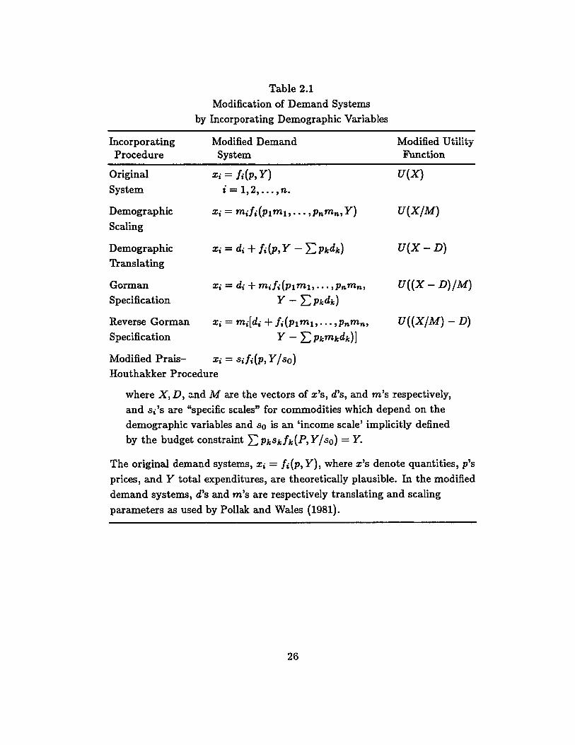
Table 2.1 presents the summary of all of these modifications of demand
systems by incorporating demographic variables.
It is obvious from the above discussion that many different theoretically
sound variants of demand systems can be permuted. However, most procedures
10 A utility function is additive if it can be written as U = E h(z,), where Ii'S are increasingfunctions of z,'s. zi's denote the quantities of the commodities into consideration.
25
IncorporatingProcedure
Original
System
Demographic
Scaling
Demographic
Translating
GormanSpecification
Reverse Gorman
Specification
Table 2.1
Modification of Demand Systems
by Incorporating Demographic Variables
Modified DemandSystem
Xi = Ii(p, Y}i = 1,2, ... , n.
Xi = di + mifdplmt, ... ,Pnmn,
Y - EPkdk}
Xi = mi[di + fi(Plmt, ... ,Pnmn,
Y - EPkmkdk}]
Modified UtilityFunction
U(X}
U(X/M}
U(X-D}
U((X - D}/M}
U((X/M} - D}
Modified Prais- Xi = sili(p, Y / so}Houthakker Procedure
where X, D, and M are the vectors of x's, d's, and m's respectively,
and s&,s are "specific scales" for commodities which depend on thedemographic variables and So is an 'income scale' implicitly defined
by the budget constraint EPkSkfk(P,Y/so} = Y.
The original demand systems, Xi = Ii(p, Y}, where x's denote quantities, p's
prices, and Y total expenditures, are theoretically plausible. In the modified
demand systems, d's and m's are respectively translating and scaling
parameters as used by Pollak and Wales (1981).
26

require price data (Prais and Houthakker, 1955; Pollak and Wales, 1979, 1980,
1981; Muellbauer, 1980; Nelson, 1988).
Where survey data provide insufficient variation in prices to identify price
effects, as frequently is the case, many studies have typically employed a variant
of Working's (1943) model (Leser, 1963; Deaton, 1982; Deaton and Case, 1987;
Deaton et al., 1989). These studies employ the Engel curves (budget share equa
tions) that best fit family budget data and are similar in specification to the form
as follows:
J
Wi = O:i + PiiIn(y/n) + ,82i[ln(y/n)r~ + L "Yijnj + c5. z (2.9)j=l
where n is the total number of family members, nj is the number of family
members in age-sex category i, and z is a vector of control variables such as age
of the head and the marker,ll their educational attainments, and employment of
adults.
More reasonable specification, which do not require price variability for iden
tification, are similar in form to equation (2.9). Such Engel curves have been
recently estimated from Spanish survey data (Deaton et al., 1989), and from Sri
Lankan and Indonesian expenditure surveys (Deaton and Muellbauer, 1986).
11 Marker is the spouse of household head; for single headed households, the head is also themarker.
27

2.4 Other Socioeconomic Studies
It is well known that children comprise a larger proportion of household members
in larger families than they do in small families. The value of children to parents
has an important social and psychological component. Indeed, the reasons for
having large families may be primarily noneconomic. Many sociological and
socioeconomic studies (for example, Leibenstein, 1954, 1957; Caldwell, 1976;
and Mangen et al., 1988) have also been done to justify the reasons for larger
family size and intergenerational relations. Still, the strictly economic analysis
of large families deserves separate study because of its bearing on the pace of
economic development.
With an objective of exploring approaches to measuring changes in family
formation levels, Schnaiberg (1973) proposes a new micro-structural measure
"child-years-of-dependency" (CYD)-with an emphasis on childrearing. CYD is
defined as one child present for one year equals one CYD, analogous to life
table person-years-lived, and asserts that we can compute CYD for the life-cycle
period of a family. He argues that the CYD measure stresses dependency, and it
is closely allied to theorizing about cost-benefit decision making about children.
He also provides some crude estimates for costs of raising children to age 18.
Household composition, rather than household size, has a significant effect
on the consumption pattern of a household. All the models and studies discussed
earlier in this chapter take into consideration only those households that have
a finite life span, such as nuclear families. But the planning horizon need not
be finite if we think of an extended family. No attempts appear to have been
made so far to apply this theory to the case of an extended family system. The
previous studies do not fill this gap because they fail to: (1) convert demographic
28

characteristics into a measurable unit for empirical analysis; (2) estimate the life
time household composition specified in the theoretical model; and (3) measure
the effect of the bequest motives on consumption patterns. This study makes an
attempt to answer those questions. The solution to the first problem is to apply
the concept of equivalence scale in our model; the solution to the second prob
lem is to analyze the fertility behavior of each household as well as their living
arrangements; and the solution to the third problem is to analyze the consump
tion behavior of extended families in an intertemporal framework by including
bequests in the utility function and the budget constraint. Theoretical construct
and model specification are discussed in the following chapter. Empirical findings
are analyzed in Chapter 6.
29

CHAPTER :1
THEORETICAL CONSTRUCT AND MODEL SPECIFICATION
3.1 Theoretical Construct
The theory of demand for many goods is well developed. Much of the theory can
be applied to the life-cycle hypothesis of consumption treating consumption in
each period as a distinct good. According to the analysis of consumer demand
theory, a consumer tries to maximize his utility subject to a given budget con
straint. If he has a well defined quasi-concave utility function Uh(X)/ where
X is the vector of n commodities, or X = (XI, X2, ••• , x n ) , where Xi is the ith
commodity available to him, and he has a fixed amount of income, Y, to spend
on these n commodities, then the objective of the consumer is to maximize
(3.1)
subject to Y = L:~=l PiXi, where Pi is the price of Xi.
Applying the method of constrained optimization, we obtain the correspond
ing demand functions for all commodities.
If we take a household as a consumer unit, then the same methodology and
procedure can be applied to determine the demand functions. This notion, how
ever, implies that either we have a glued-together family having identical tastes,
or the household decision function is dictatorial (despotic head). If so, there is
no problem with (3.1). As a group, a household is a small closely knit collection
1 A utility function is quasi-concave if its indifference curves are convex to the origin.
30

of individuals. Yet there is a problem that has to be handled when trying to
find empirically applicable demand functions for a household. The problem is
to converting demographic variables into a measurable unit. To overcome this
problem this study applies the method of "equivalent adults."
Let us define some of the terms that are used in this study. Head refers to
the household head unless otherwise stated, and households are represented by
their heads. Bequests are household assets left at the final period of the life span
of the head." Similarly, inheritances are household assets that were inherited by
the head from his predecessor(s).
We assume that our representative household has a well defined quasi-
concave utility function. The budget of the household is constrained by its
lifetime resources. The household will make its intertemporal consumption de
cisions based on the postulation that its utility function is maximized subject to
the budget constraint.
Time preference is defined as the human desire for present consumption as
opposed to future consumption. The desire is reflected by the price people are
willing to pay for immediate consumption as opposed to the price they are willing
to pay for future consumption. A positive rate of time preference indicates that
current consumption is preferred to future consumption. The rate is negative if
the converse is the case.
2 Decease, abdication, retirement, or any other reason could be the cause of the end of thelife span of the household headship.
31

3.1.1 The Utility Function
We assume that the utility function is additive and separable." We also assume
that in extended family systems household heads derive utility from bequests and
intend to bequeath some assets to their offspring. Therefore, bequests appear as
an argument in the household utility function. Let U(BL) be the utility derived
from leaving BL as bequests. Then the lifetime utility of the household (in terms
of present value), which is the sum of all utilities derived throughout its life
period, will be
(3.2)
where Ct and mt are total consumption and number of equivalent adults respec
tively; Ct = (Ct/mt) denotes anticipated consumption per equivalent adult; f(Ct)
is the utility derived from it, all measured at time t; and p denotes the rate of
time preference. In this model the household is represented by the age of the
household head, T + t. The limits of integration T and L are the ages of the
household head at the beginning of his planning horizon and his terminal age.
Therefore, t refers to t period(s) later in the future.
Households seem to display a positive rate of time preference. That is,
they tend to place a higher subjective value on consumption in the near future
than on consumption in the more distant future. This rate also differs across
socioeconomic classes. Lawrance (1991) argues that poor households are likely to
possess relatively high rates of time preference and, consequently, relatively high
3 The additivity assumption implies that the marginal utility of consumption at any timeperiod is independent of the consumption at any other period. The additive separabilityassumption allows us to treat different aspects of utility separately from each other.
32

(3.3)
marginal propensity to consume implying very different patterns of consumption
over the life-cycle. IT households have reason to believe that their income will
increase over time, they could very logically conclude that giving up something
now entails a larger subjective sacrifice than giving up quite a bit more of the same
thing at a future date when they expect their income to be greater. Therefore,
I have incorporated the concept of rate of time preference into my model.
3.1.2 The Budget Constraint
The budget constraint for intertemporal consumption can be expressed in terms
of present value or future value. For this study, I will express the budget con
straint in terms of present value.
The budget of a household is constrained by its lifetime resources, includ
ing inheritances. The present value of total lifetime resources of a household
anticipated from his current age T, VT, is
VT = AT +LL yte-rtdt
where yt is the household income at time t, and T is the rate of discount.
The first term of the right hand expression, AT, is the value of the house
hold's initial holding of assets, including inheritances. The second term is the
sum of all discounted future income, including the earnings of all household mem
bers. It is difficult to estimate accurately the value of this term; however, we can
estimate it by following the technique prescribed in Modigliani and Brumberg
(1954: 396). If ytc is the expected average annual discounted income at period
t, then
33

"Yte = hL
Yte-rtdt/ET
where ET = (L - T) is the remaining life span of the household. This is the
head's life expectancy at age T.
Or alternatively,
LL Yte-rtdt = ETY{.
If we further assume that the income grows annually at some constant rate,
say g, then
where YT is the current income of the household (income at age T). Then we
have
LL Yte-rtdt = ETYTegt.
Substituting this value in (3.3), we get
(3.4)
If the values of AT, E T, YT, and 9 are known then the present value oflifetime
resources (i.e., VT) is also determined.
Given the household lifetime resources, the household has to make intertem
poral consumption decisions that are affordable throughout its life-cycle. The
household would spend some of these resources on its lifetime consumption and
34
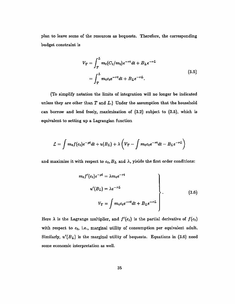
plan to leave some of the resources as bequests. Therefore, the corresponding
budget constraint is
VT = LL mt(Ct/mt)e-rtdt + BLe-rL
= LL mtcte-rtdt + BLe-rL.(3.5)
(To simplify notation the limits of integration will no longer be indicated
unless they are other than T and L.) Under the assumption that the household
can borrow and lend freely, maximization of (3.2) subject to (3.5), which is
equivalent to setting up a Lagrangian function
and maximize it with respect to Ct, BLand A, yields the first order conditions:
(3.6)
Here A is the Lagrange multiplier, and f'(ct) is the partial derivative of f(Ct)
with respect to Ct, i.e., marginal utility of consumption per equivalent adult.
Similarly, U'(BL) is the marginal utility of bequests. Equations in (3.6) need
some economic interpretation as well.
35

Using the Envelope theorem, Acan be interpreted as the derivative of U with
respect to VTi therefore, A is the marginal utility of (discounted) resources. The
first equation in (6.3) says that at every point along the optimal consumption
path, the discounted marginal utility of per adult consumption equals the present
value of an extra unit of resources. Similarly, the second equation says that this
present value of an extra unit of resources should equal to the marginal utility
of bequests. The third equation asserts that the budget constraint represented
by (3.5) should always be satisfied at every point along the optimal consumption
path. Solving the equations in (3.6) we can derive the corresponding consumption
function.
3.2 Model Specification
3.2.1 Theoretical Model
If we know the specification of the household's utility function, we can obtain a
clearer picture of the optimal consumption path. Since we can subject a utility
function to any monotonically increasing transformation without affecting the
nature of its demand functions but will simplify our problem," we shall take the
logarithm of this function. Therefore, let f(Ct) = c ln c., and U(BL) = ablnBL.
Here a and ab denote the elasticities of utility with respect to consumption and
bequests respectively. Then the first order conditions for utility maximization,
as shown by equation (3.6), can be written as
4 See, for example, Silberberg (1990: 311) for the proof of this assertion.
36

(3.7)
From (3.7) it is simple to show that
C - c e(r-p)tt - 0 •
Substituting Ct = Ct!mt, we get
(3.8)
Equation (3.8) shows that consumption per equivalent adult grows at a constant
rate (r - p), whereas total household consumption also depends on household
composition. Comparing consumption at two different time periods i and i, we
haveCi _ mi (r-p)(i-j)
C-.e .
j mj
From (3.9) it also follows that
(3.9)
(3.10)
This gives us the household consumption path over time. The rate of time
preference, p, together with the market rate of discount, r, is needed to make
37

intertemporal consumption decisions. A comparative statics analysis shows that
depending upon the values of p and r the household can reallocate its consump
tion over its life-cycle. If r is greater than p, then future consumption (total as
well as per equivalent adult) will be greater than present consumption, whereas
the reverse will follow if r is less than p, Equations (3.8) and (3.10) also show that"
the relative consumption paths (total and per equivalent adult) are independent
of consumption elasticity and the bequest elasticity (a and ab respectively).
From (3.7) and (3.10) it follows that
(3.11)
Substituting the values of Ct from (3.10) and B L from (3.11) into (3.5), the
budget constraint will be
Therefore,
c, (X )mte(r-p)t
VT - (X)[! mte-ptdt + b]
(3.12)
Alternatively,
(3.13)
38

This model shows that the fraction of lifetime resources consumed at any age of
the household is approximately equal to the ratio of equivalent adults at that age
to the sum of lifetime equivalent adults and the bequest motives. Put it differ-
ently, if the household can forecast lifetime resources, lifetime equivalent adults
including the bequest parameter, then it will allocate consumption consistent
with its demographic profile. Any change in the demographic profile, therefore,
directly influences the pattern of consumption.
Equation (3.13) can be rewritten as
(3.14)
This is a Fisher-type (1956) specification of consumption function. My specifi
cation differs from his in the sense that I have allowed for bequests in my model,
whereas he has not. Fisher's specification is a special case of my specification
when b = O. This functional form needs some interpretation as well.
The left-hand side represents the household consumption at period t dis
counted to present time. Note that T, the age of the household head, is the
current time (or the initial period) in this analysis.
On the right-hand side, the numerator of the coefficient of VT (i.e., mte-pt)
denotes the number of equivalent adults at time t (but discounted properly)
to present time T. Likewise, the denominator represents the total number of
equivalent adults in the family's entire life-cycle, including bequests. It should
be noted that b has the same unit (years of adult equivalent consumption) as mt
has. It can be interpreted as the number of equivalent adult years of consumption
39

that an average family leaves as a bequest. Obviously, bequest does not appear
as a variable in this model.
3.2.2 Econometric Model
Rearranging equation (3.13), we get
where M t = Jmte-ptdt + b. Focusing the consumption on the current period T
implies
c= (~)V. (3.15)
The complete theoretical model is specified by substituting the value of VT
from equation (3.4) in equation (3.13) to obtain
c = (~) [A + E(1 +g)Y] (3.16)
where expected income differs from unexpected income by a small fraction g.
Divide this equation by Y to get
C (m) A-= - [-+E(I+g)].Y M Y
Taking the natural logarithm of this equation yields
In (~) = In (;;) + In[¢ + E(l + g)].
40
(3.17)

If we switch from continuous to discrete formulation, then the fully specified
econometric model for the empirical purposes can be written as
I (C) I ( klNI + k2N2 + kaNa + k4N4 )n y. - n klSNI + k2SN2 + kaSNa + k4SN4 + b
A+ In[ks(y) + ksEl(3.18)
where Nl, N2' N s, and N4 are the numbers of children of ages 0-9, teenagers
10-19, adult males, and adult females respectively; SNI, SN2, SNa, and SN4 are
their respective expected lifetime numb...rs discounted by the rates of time pref-
erence. If we constrain kg equal to one, then kl, k 2 , and k4 can be interpreted as
equivalent male adult consumption by children of ages 0-9, teenagers, and adult
females; ks is the effect of the net assets-current income ratio on consumption; ks
is the growth rate of future income measured as the effect of the household's life
expectancy on consumption; and b can be interpreted as the number of equiva-
lent adult years of consumption that an average family leaves as bequests. Note
that bequest does not appear as a variable in this model.
Equation (3.18) is the fully specified empirical model of life cycle consump
tion. The model shows that the consumption ratio, C/Y, consists of two parts.
The first part of the right hand side expression can be viewed as the demographic
component of the consumption model, and the second part can be viewed as the
economic component. The values of the variables C,A,Y,NI,N2,Ng , and N 4
are available from the household survey; E can be calculated from the age and
the life expectancy of the head; and SN1 , SN2, SNa, and SN4 are determined by
the future household composition. Projection of future household composition is
described in Chapter 5.
41

IT we assume that 9 = 0 then theoretically k 5 and k6 will have same pa
rameter. Therefore, a separate model is estimated by constraining k 5 = k6 • The
rationale for imposing this constraint is that, because we are assuming that 9 is
small, the hypothesis that 9 = 0 is tested by this constrained model.
The introduction of demographic factors modifies the model in such a way
that the marginal propensity to consume depends upon the number of equivalent
adults relative to future lifetime equivalent adults (m/M). It should be noted,
however, that expected demographic profiles (lifetime equivalent adults, M) will
be revised for each period to incorporate new information and to reflect the
probability distribution of future household composition.
42
CHAPTER 4
HOUSEHOLD SURVEY
Empirical research is needed to fulfill our objectives and to estimate the equa
tion specified in the preceding chapter. Accordingly, a data set on household
composition, socioeconomic variables, income, and expenditures is required.
Choosing between a cross-section and a time-series study is the first problem
for such a study. A cross-section study is the analysis of data collected from a
population at a period in time, which purports to represent the state of affairs
prevailing in the population at that moment. Time-series analysis is the statis
tical analysis of a series of repeated observations of the same variable, or, in the
case of multiple time-series analysis, a set of variables.
Ideally, a life-cycle model requires a set of time-series data on household
composition, consumption expenditures, lifetime income, savings, and net worth
for a period covering the households' entire life span. Nepal is poor not only
in material things but also in research data. It does not have a well-developed
statistical system nor a long tradition of survey analysis. It is also very expensive
to do panel studies. Since such data are not available for Nepal, a field study was
conducted by me during the period of 1987-88 to collect data on the demographic
and economic characteristics of households. This chapter presents the salient
features of my field survey (Kanel, 1988), which is cited as Household Survey,
1987-88.
43

4.1 Location, and Method of Data Collection
Kathmandu was selected as the field location for this study. The criteria for
selecting Kathmandu as the field site are fairly obvious. First, Kathmandu, the
capital city of Nepal, is the most cosmopolitan city in Nepal. Therefore, it would
not be difficult to include households with different socioeconomic characteristics
in my sample. Second, Kathmandu has a more monetized economy than other
areas of Nepal. Thus, it is easier to get information on income, assets, and expen
ditures. Third, because of a better transportation and communication system
than elsewhere in the country, it is easier to work in or near Kathmandu. Gov
ernment offices and organizations, research institutions, libraries, and academic
intelligentsia cannot be better available elsewhere in Nepal than in Kathmandu.
Information was collected by both household survey as well as through sec
ondary sources. The primary method of household survey was structured inter
views. A pretested questionnaire translated into the Nepali language was taken
to the field site. Information was collected on economic (income and expenditure
patterns), demographic (family size and composition, information on nuptiality,
and desired family size), and socioeconomic status (ethnicity, mother tongue,
educational attainment, and occupation) of household head and its members. A
questionnaire was designed to capture necessary information for this purpose.
The Freedman and Mueller (1977) module was used as the basic guideline while
designing the questionnaire. Nevertheless, several modifications and changes
were made in the module to satisfy the data requirements for this study. The
questionnaires were translated into the Nepali language and redesigned after a
44
pretest to avoid any ambiguity and obscurity in the questions. 1 The question
naire used in the field is attached as an Appendix to this dissertation. Data on
national and district levels are taken from published sources.
Households are the units of analysis for this study. The main objective was
to interview a. sample of households of Kathmandu Valley. Since there was no
complete up-to-data list of all households, it was necessary to draw a sample of
all Kathmandu households. This was not possible because of financial and time
constraints. Therefore, it was necessary to select a small sample.
Household survey was designed to obtain data on demographic and eco-
nomic variables for a sample representing all non-institutional households in
Kathmandu. The survey methodology as described in Palmore (1969) has been
followed and employed as the basic guideline while conducting field survey," This
section provides a brief description on the survey methodology.
The household survey is based on a sample of all non-institutional households
in Kathmandu. The sample size was set to a reasonable level so that reliable
estimates of population parameters could be made. This average level was set
at about 700 households so that my sample would have 600 households at the
minimum. Three enumerators were temporarily hired to help me interview the
selected households.
In order to arrive at a sufficient sample of intensive interview with household
heads, it was necessary to visit more households than the number of interviews
wanted. Although the goal was to obtain about 700 interviews in total, 800 sam-
ple addresses were selected in the sample to allow for losses due to no-responses
1 I did a pretest of twenty households before the actual survey was conducted.
2 A more detailed discussion on the survey methodology is in National Family PlanningBoard (1966-1967), Report on West Malaysian Family Su.rfJey: 1966-1967.
45

and incompletes. Even though there was no firm factual basis to support the
initial estimate that a sample size of 800 would yield to a minimum of 600 inter
views the survey yielded a total of 614 intensive interviews which was within the
target range."
To save time and travel costs during the field study, the sample space con-
tained of a judgment sample of 40 blocks of 20 households each. These blocks,
which included rural as well as urban households with different socioeconomic
characteristics, were selected from different parts of the Kathmandu valley. The
actual sample of households was drawn starting at a random point in a complete
listing of all households in the sample blocks and a systematic random sample
was taken from that point on.
Our interview basically concentrated on the household head or his spouse,
who had better knowledge about household income and expenditures as well as
household demographics. Sometimes, we could not find either of them. In such
cases, we revisited the household for interviewing. Ifneither of them was available
even on the second visit, we asked another adult member of the household to
respond to our questions and collected information from that respondent. If that
member could not answer all of the questions in the questionnaire, we omitted
that household from our list and interviewed a neighboring household instead.
On the average, each interview lasted about one hour and thirty minutes.
The survey was conducted from November 1987 to March 1988 in all three
districts of the Kathmandu Valley," All households were interviewed personally
and responses were recorded in structured questionnaires. Every effort was made
3 Incidentally, this number is 0.5 percent of the total households of Kathmandu Valley asof the 1981 census.
4 A district is an administrative unit, and there are 75 such districts in Nepal. Kathmandu,l.alitpur, and Bhaktapur-all in Kathmandu Valley-are three of them.
46
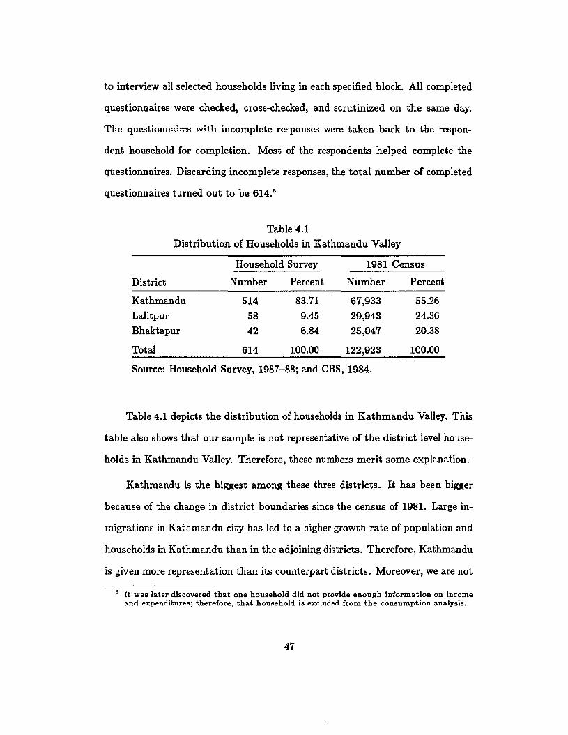
to interview all selected households living in each specified block. All completed
questionnaires were checked, cross-checked, and scrutinized on the same day.
The questionnaires with incomplete responses were taken back to the respon-
dent household for completion. Most of the respondents helped complete the
questionnaires. Discarding incomplete responses, the total number of completed
questionnaires turned out to be 614. 6
Table 4.1Distribution of Households in Kathmandu Valley
Household Survey 1981 Census
District Number Percent Number Percent
Kathmandu 514 83.71 67,933 55.26
Lalitpur 58 9.45 29,943 24.36
Bhaktapur 42 6.84 25,047 20.38
Total 614 100.00 122,923 100.00
Source: Household Survey, 1987-88; and CBS, 1984.
Table 4.1 depicts the distribution of households in Kathmandu Valley. This
table also shows that our sample is not representative of the district level house
holds in Kathmandu Valley. Therefore, these numbers merit some explanation.
Kathmandu is the biggest among these three districts. It has been bigger
because of the change in district boundaries since the census of 1981. Large in-
migrations in Kathmandu city has led to a higher growth rate of population and
households in Kathmandu than in the adjoining districts. Therefore, Kathmandu
is given more representation than its counterpart districts. Moreover, we are not
6 It was later discovered that one household did not provide enough information on incomeand expenditures; therefore, that household is excluded from the consumption analysis.
47

interested in doing any comparative analysis across districts; therefore, this dis
tribution of surveyed households should not really matter. Otherwise, we could
have calculated and used a proper weight to take care of the over-representation
of Kathmandu and the under-representation of Lalitpur and Bhaktapur. The
purpose of reporting this table is to present an overview of the household distri
bution in Kathmandu Valley.
Table 4.2Age Distribution of Household Heads
Age Number Percent
15-19 1 0.1620-24 11 1.7925-29 37 6.0330-34 72 11.7335-39 57 9.2840-44 83 13.5245-49 59 9.6150-54 85 13.8455-59 66 10.7560-64 56 9.1265-69 29 4.7270-74 25 4.0770+ 33 5.37
Total 614 100.00
Source: Household Survey, 1987-88.
Life-cycle analysis of household composition and family consumption be
havior requires that the survey cover various ages of household heads. Table
48

4.2 presents a quinquennial sample distribution of age of heads. These num
bers could not be compared with the national or district level numbers, because
census or published figures on such data are not available.
4.2 Household Characteristics
Household characteristics include household type, and the size and composition
of the household. It often includes education and occupation of the household
members (including the head), and their relationship to the head. Differences
in household characteristics affect the consumption pattern of a household over
time and across households at a period in time. This section describes the char
acteristics that affect the household consumption decisions, although we have
not explicitly included all of these factors into our model.
4.2.1 Household Types
Four types of households are distinguished: (1) intact households, households
headed by a male with the spouse present; (2) single-headed households, house
holds in which the head's spouse is not present; (3) one-person households; and
(4) primary-individual households, households consisting of unrelated members.
The distribution of households according to their types is presented in Table 4.3.
Of the households sampled, 99.35 percent are family households (Table 4.3).
Only four households in the sample are primary-individual households. Of the
610 family households, 298 (48.85 percent) are nuclear and 312 (51.15 percent) are
extended. Households with no members other than a head, a spouse, unmarried
children (including adopted children), or helpers/servants are defined as nuclear
households. On the other hand, households where three or more generations live
49

Table 4.3
Distribution of Household Types
Household Type Number Percent
Family households
Intact 501 81.60
Single-head
Male 48 7.82
Female 61 9.93
All family households 610 99.35
Nonfamily households
Primary-individuals
Male 4 0.65
Female 0 0.00
One-person 0 0.00
All nonfamily households 4 0.65
All households 614 100.00
Sex of household head
Male 553 90.07
Female 61 9.93
All family households
Extended 312 51.15
Nuclear 298 48.85
Source: Household Survey, 1987-88.
together are extended households. This category also includes households with
joint families. Family households not otherwise included in nuclear households
are also a component of extended family households. There are no one-person
households in our sample.
As a typical household begins its life-cycle, its size will increase from two
to more with births and adoptions. However, a new household formed out of an
50

extended and/or joint family household can begin with any number of members.
New members will appear in the household, and the household will continue to
grow until a member dies or departs from the household, or a split-up occurs in
the household. Table 4.4 shows the distribution of household size in Kathmandu.
Table 4.4
Distribution of Household Size
Household Survey 1981 Census
Persons Number Percent Number Percent
1 0 0.00 5,314 4.32
2 13 2.12 8,237 6.70
3 32 5.21 10,696 8.70
4 91 14.82 15,453 12.57
5 114 18.57 18,617 15.15
6 109 17.75 17,618 14.33
7 79 12.87 14,159 11.52
8 59 9.61 10,082 8.20
9 30 4.89 8,828 7.18
10 29 4.72 3,520 2.86
11+ 58 9.44 10,399 8.47
Total 614 100.00 122,923 100.00
Source: Household Survey, 1987-88; and CBS, Nepal, 1984.
Table 4.4 reports a comparative distribution of household size as shown from
the household survey and the 1981 census. The table shows that the survey data
do not represent the household composition (household size and age-sex struc
ture) of Kathmandu. Various remedial procedures are suggested to take care of
such a situation when a sample seems to be non-representative of the population.
One method is to assign proper weights on sample observations depending upon
51

specific characteristics of the observations provided that we have enough infor
mation on both the population and the sample regarding those characteristics.
Using my sample and the 1981 census figures for the Kathmandu valley a new
weight variable is calculated, following Kalton (1983), from the age distribution
of household population and the distribution of household size. This weight is
later used to analyze our data and draw statistical inferences therefrom.
My survey showed a total of 4,075 persons in 614 households. The average
household size is 6.6 members with median 6 and mode 5. This indicates that
the distribution is positively skewed, which is consistent with what one would
expect in a growing population. The average household size for Kathmandu and
Nepal, according to the 1981 census, are 6.3 and 5.8 respectively (CBS, Nepal,
1984).
Table 4.5
Marital Status of Household Heads
Status Number Percent
Never been married
Currently married
Widow/WidowerSeparated
Divorced
No Response
Total
7
501
97
1
o8
614
1.14
81.60
15.80
0.16
0.00
1.30
100.00
Source: Household Survey, 1987-88.
Of the total 614 households, there are 501 (81.60 percent) intact households,
where both the head and the spouse are present (Table 4.3). Sixty-one (9.93
percent) households are headed by single females (with no spouse present), and
52

48 (7.82 percent) households by single males. Table 4.5 shows the marital status
of the heads of surveyed households. More than 80 percent of the heads are
currently married.
Table 4.6
Average Number of Household Members
by Their Relationship to the Household Head
Relationship Averageto Head Number Percent
Head 1.00 15.07
Spouse 0.83 12.54Children(a) 2.76 41.64Parents (a) 0.08 1.23
Grandchildren 0.85 12.79
Daughters-in-law 0.44 6.70
Brothers and Sisters 0.18 2.67
Brothers/Sisters-in-Iaw 0.04 0.66
Other Relatives(b) 0.15 2.33Others(c) 0.22 3.36
No Response 0.07 1.01
Total 6.64 100.00
Source: Household Survey, 1987-88.
a Adopted children are included in children, and parents-in-law
in parent categories.
b "Other relatives" includes all relatives excluding those that
have otherwise been included.
c "Others" includes non-relatives such as friends, helpers
and servants.
Table 4.6 depicts the family relationship among household members. Of the
6.64 persons per household, every household has one, and only one, head. The
average number of spouses per household is 0.83. This is because some of the
53

heads do not have their spouses." The remaining members are children of the
head (2.76), parents (0.08), grandchildren (0.85), daughters-in-law (0.44), broth
ers and sisters (0.18), brothersfsisters-in-Iaw (0.04), other relatives (0.15), and
others (0.22). Since "others" constitute a very small proportion of the house
hold members, it also reconfirms that "household" and "family" can be taken as
equivalents in Nepal.
4.2.2 Ethnicitv and Mother Tongue of Heads
Nepal is the only Hindu country in the world. It consists of many ethnic groups,
and different castes. Ethnicity, in the present context, is loosely defined and is
associated more with caste. Some of the heads did not specify their caste, but
gave only their religion as "Hindu". Hindu religion includes Brahmans, Chhetris,
and many other ethnic groups.
There are many languages spoken in Nepal but Nepali is the only official and
national language. It is spoken and understood by almost all people. However,
different ethnic groups have their own mother tongue. Table 4.7 is a cross-
tabulation that shows the ethnicity of households with their mother tongues.
Table 4.7 illustrates that there is a strong association between ethnicity and
mother tongues. It also points some interesting features. Brahman and Chhetri's
mother tongue is always Nepali (except for those two Chhetri households who
told us during the interview that they had just in-migrated from the Terai where
they used to speak Bhojpuri). The proportion of households having their mother
6 It should also be noted that some people in Nepal have more than one wife. There were9 household heads in my sample who have two wives. In such cases, the wife whose ageis most close to the husband's age is designated as wife, which will supposedly betterexplain the life-cycle behavior of the household, and the other wife is designated as "otherrelative" .
54

Table 4.7
Ethnicity and Mother Tongue of Households
Mother Ethnicity
Tongue Brahman Chhetri Newar Hindu* Others] All
Nepali 222 166 21 40 28 477
Newari 0 0 119 0 0 119
Othersf 0 2 0 3 13 18
Total 222 168 140 43 41 614
(0.36) (0.27) (0.23) (0.07) (0.07) (1.00)
Source: Household Survey, 1987-88.
Note: Numbers in parentheses indicate the proportion of households
in the given category.
* Those who preferred to call themselves Hindu.
t Includes Gurungs, Tamangs, lower castes, and Muslims.
t Includes Tamang, Maithili, Bhojpuri, and Urdu.
tongue other than Nepali and Newari is very small in Kathmandu. Newari is the
mother tongue of Newars only. Only 3 percent of the households have a mother
tongue other than Nepali or Newari. About 93 percent of the households belong
to either the Brahman and Chhetri clan, the Newar group, or (as th.ey chose to
call themselves as) Hindu.
4.2.3 Educational Attainment of Heads
In Nepal, education falls into four general categories: primary (grade 1 to 5),
lower secondary (middle school, grade 6-7), secondary (high school, grade 8
10), and higher education (college and university). The new education plan,
which introduced vocational education at school level," was introduced in 1972.
7 In Nepal "school" implies until high school only. After tha.t they are called colleges oruniversities.
55

Primary education is now compulsory, and tuition and books are free for grades
1 through 3. Beyond primary education, moderate tuition charges are levied
in public lower secondary and secondary schools. The 1972 plan introduced
an American-type of semester system (two semesters in one year) in the higher
education level. In 1981 the semester system was replaced by British-type annual
system.
The literacy rate of Nepal is only 23.5 percent, according to the 1981 census.
The census also shows that literacy rate for Kathmandu is 49.0 percent, Lalitpur
36.3 percent, and Bhaktapur 32.0 percent. Recently this rate is increasing every
year. Table 4.8 presents the years of schooling of all household members and
heads under our present study.
Table 4.8
Educational Attainment of Heads and Members
Years of Heads Members
Schooling Number Percent Number Percent
llliterate 103 16.78 949* 23.29*
Literate Only 172 28.01 870 21.35
Q-4 0 0.00 345 8.47
5-7 9 1.47 210 5.15
8-10 92 14.98 782 19.19
11-14 142 23.12 655 16.07
15+ 93 15.15 238 5.84
No Response 3 0.49 26 0.64
Total 614 100.00 4075 100.00
Source: Household Survey, 1987-88.
* This includes children under school age.
56

Table 4.8 shows that proportionately more heads are literate and educated
than is the case for the general population. This is a plausible observation be
cause the total population includes small children and aged persons who are
proportionately more illiterate than the young population. About 67 percent
of the respondents are literate. This higher literacy rate could be because of
an increase in the literacy rate of Kathmandu's population, or due to a high
proportion of urban population in our sample, or due to large in-migration of
literate and educated population in Kathmandu, or any combination of the above
factors. This increase in the literacy rate seems to be plausible.
4.2.4 Occupation of Heads
The occupation of a household head is the major type of work performed by the
person at his/her principal job. The occupation of a head is recorded as answered
by the respondent.
Unlike other capital cities, Kathmandu has a substantial proportion of its
population engaged in agriculture. There are some special caste groups of people
whose traditional occupation is agriculture. Households with little or no educa
tion and a very low opportunity cost engage in agriculture, producing especially
vegetables. It is a very profitable business because of the soaring prices of green
vegetables in Kathmandu.
Table 4.9 shows the distribution of occupations of household heads. Farm
ers constitute the second largest group after office employees. Civil servants
and other employees in offices and institutes constitute 40.55 percent of the to
tal heads. The proportion of the population in other professions (journalists,
lawyers, engineers, and medical doctors) constitutes only 0.81 percent. Retirees
57

*
Table 4.9
Occupation of Household Heads
Type ofOccupation Frequency Percent
Agiculture 106 17.26
Housewives 76 12.38
Wage-earners 6 0.98Employees 249 40.55
Students 4 0.65
Business 90 14.66
Politics 8 1.30
Industry 6 0.98
Retired 21 3.42
Professionals* 5 0.81
Teaching 21 3.42
Unemployed 5 0.81
Others** 15 2.44
No Response 2 0.33
Total 614 100.00
Source: Household Survey, 1987-88.
This includes journalists, lawyers, engineers,
and medical doctors.
** This includes shoemakers, butchers, priests,
tailors, drivers, masons, and blacksmiths.
and most female heads, accounting for 12.38 percent, stay home and take care
of the children and the household.
4.3 Household Income, Expenditures, and Net Assets
Data were collected on household income, expenditures, and the net assets of
all households. One household did not provide enough information on income
58

and expenditures; therefore, the total number of households answering these
questions is 613.
Household income is the sum of (1) wages and salaries, tips, bonuses, pen
sions, etc.; (2) net profits from farming and non-farming activities; (3) property
income, such as land rent, house rent, royalties, interest, and dividends; (4) trans
fer payments received, such as assistance payments, scholarships, and grants; (5)
income-in-kind - the value of goods and services received as part of pay, home
produced and consumed (including the rental value of owner-occupied and free
dwellings), or received free from other sources; and (6) other money receipts such
as insurance proceeds, lottery winnings, and other windfall receipts. Household
total disposable income is the total household income minus taxes paid.
Household expenditures are total household expenditures, which include (1)
the amount spent to purchase goods and services used for living purposes; (2)
the value of goods and services received as part of pay, home-produced and con
sumed (including rental value of owner-occupied and free dwellings), or received
free from other sources; and (3) the amount spent for contribution, insurance
premiums, lottery tickets, interest on debts, and other non-consumption items.
Non-monetary income (such as children's contribution and adults' involvement in
housework), the value of exchange labor, and the rental value of owner-occupied
houses and free housing have also been taken care of by including them both in
income and expenditures when calculating household income and expenditures.
All incomes and expenditures are annual.
The net assets of a household are defined as the difference between total
assets and total liabilities (debt). Therefore, unlike income and expenditures, it
59
is a stock variable. All tangible property including household durables are total
assets. Any debt that a household might have to repay is the liability.
4.3.1 Household Income
Questions about household (or personal) income are very sensitive. People do
not want to reveal their income. It is also very difficult to obtain accurate figures
for countries like Nepal where the economy is not fully monetized, and some
sort of barter system, in one form or another, still exists. Vegetables grown in
the backyard for one's own consumption, a poultry farm with a couple of birds
only for the household consumption of eggs, and some unpaid work rendered by
friends and relatives, for example, not only create a problem of valuation for such
goods and services but also underestimate the income of the household, at the
micro level, and the gross domestic product (GDP), at the macro level. We tried,
however, to capture all sources of income by asking different questions, including
the sources and valuations of non-monetary income and the subjective monetary
valuation of the housework done by its members. Table 4.10 shows the annual
income distribution of households.
4.3.2 Household Expenditures
Collecting accurate information on household expenditures is also very difficult
especially because a high proportion of goods and services are non-monetized.
People grow and consume their own food, and drink milk from their own buffaloes
or cows and do not keep track of these items. Some households do not even know
the exact volume or value of their production. As in the case of household income,
however, we tried to capture an different forms of household expenditures. Table
60
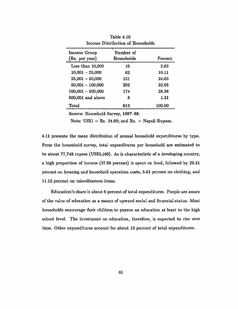
Table 4.10
Income Distribution of Households
Income Group(Rs. per year)
Less than 10,000
10,001 - 25,000
25,001 - 50,000
50,001 - 100,000
100,001 - 500,000
500,001 and above
Total
Number ofHouseholds
16
62
151
202
174
8
613
Percent
2.62
10.11
24.63
32.95
28.38
1.31
100.00
Source: Household Survey, 1987-88.
Note: US$l = Rs. 24.60; and Rs. = Nepali Rupees.
4.11 presents the mean distribution of annual household expenditures by type.
From the household survey, total expenditures per household are estimated to
be about 77,748 rupees (US$3,160). As is characteristic of a developing country,
a high proportion of income (37.89 percent) is spent on food, followed by 29.21
percent on housing and household operation costs, 5.61 percent on clothing, and
11.12 percent on miscellaneous items.
Education's share is about 6 percent of total expenditures. People are aware
of the value of education as a means of upward social and financial status. Most
households encourage their children to pursue an education at least to the high
school level. The investment on education, therefore, is expected to rise over
time. Other expenditures account for about 10 percent of total expenditures.
61

Table 4.11
Distribution of Annual Expenditures
[Per Household)
Items Amount (Rs.) Percent
Food tHousing and housing
operating cost tEducation
Clothing
Medical care
Transportation
Entertainment and
recreation
TaxSocial activities andreligious ceremonies
Miscellaneous
Total
29,459
22,709
4,647
4,363
1,709
2,238
1,172
498
2,309
8,645
77,748
37.89
29.21
5.98
5.61
2.20
2.88
1.51
0.64
2.97
11.12
100.00
Source: Household Survey, 1987-88.
t Food includes market and non-market transactions.
t Includes rental value of owner-occupied houses.
4.3.3 Household Net Assets
Because many people do not want to reveal their income, any question regarding
income and assets is sensitive. Therefore, data on household net assets may be
unreliable.
Table 4.12 shows the distribution of the net assets of Kathmandu house-
holds. Land, houses, and household items are the major household assets. Of
the households surveyed, about 52.69 percent have a net wealth of more than
62

Net Assets(in Rs.)
Table 4.12
Household Net Assets
Number ofHouseholds Percent
Less than 10,000
10,001 - 25,000
25,001 - 50,000
50,001 - 100,000
100,001 - 500,000
500,001 - 1,000,000
1,000,001 and above
Total
53
15
2829
165
131
192
613
8.65
2.454.56
4.73
26.92
21.37
31.32
100.00
Source: Household Survey, 1987-88.
500,000 rupees (US$20,325). The mean value of these net assets is about 950,000
rupees (US$38,617) per household.
Table 4.13 summarizes the average income, expenditures, assets, and sav-
ings of the surveyed households. The table shows that the average income per
household is about 95,711 rupees (US$3,890) per year," Because the average
number of persons per household is 6.6, the average annual income per capita for
the surveyed households is 14,502 rupees (US$590). This is significantly higher
than the GNP (Gross National Product) figure for 1989 of US$160 (World Bank,
1989: 164-165). This "high income" is probably the result of four factors. The
first factor is that more rich people live in Kathmandu. The second factor is that
more people live in urban areas and are employed, and therefore, earn a regular
salary. The third factor is that people exaggerate their income and expenditures.
The fourth factor is that the GNP is calculated in a somewhat different way. It
8 The average exchange rate during the period of household survey W2.S 24.60 rupees per USdollar.
63

comprises gross domestic product plus net factor income from abroad, which is
the income residents receive from abroad for factor services (labor and capital)
less similar payments made to nonresidents who contributed to the domestic
economy. Of this total earnings, about 34.30 percent is from business profits,
31.31 percent from salaries and wages, 13.21 percent from agriculture, and 21.18
percent from other sources.
Average total expenditures per household are 77,748 rupees (US$3,160). The
general tendency of the respondents, when asked about their income-expenditure
amounts, was to overstate expenditures. Therefore, the amount of average ex
penditures seems to be high; and savings seems to be low. When asked directly
about their savings or dissavings during the past 12 months, 289 household heads
(47.07 percent) asserted an amount of dissavings and 294 heads (47.88 percent)
said that their income and expenditures would just break-even. The calculation
of their balance sheet showed some savings. It means people are either exaggerat
ing their income, or they are just not being honest when answering the questions
regarding income and expenditures.
4.4 Inheritances and Bequests
Inheritances and bequests are two different sides of the same coin. Inheritances
are defined as the property and household assets received by a head from his
predecessor, whereas bequests are the property and household assets left by a
household head, at the time of death, to his successor. Whatever is inherited
by recipients is the bequests of their bestowers. Inheritances and bequests occur
almost universally in Nepal. According to the tradition and culture, sons inherit
the property and wealth of their parents and grandparents, even though recent
64
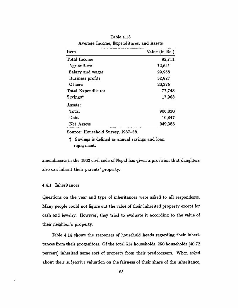
Item
Table 4.13
Average Income, Expenditures, and Assets
Value (in Rs.)
Total Income
Agriculture
Salary and wages
Business profits
OthersTotal Expenditures
Savings]
Assets:
Total
Debt
Net Assets
95,711
12,641
29,968
32,827
20,275
77,748
17,963
966,830
16,847
949,983
Source: Household Survey, 1987-88.
t Savings is defined as annual savings and loanrepayment.
amendments in the 1962 civil code of Nepal has given a provision that daughters
also can inherit their parents' property.
4.4.1 Inheritances
Questions on the year and type of inheritances were asked to all respondents.
Many people could not figure out the value of their inherited property except for
cash and jewelry. However, they tried to evaluate it according to the value of
their neighbor's property.
Table 4.14 shows the responses of household heads regarding their inheri
tances from their progenitors. Of the total 614 households, 250 households (40.72
percent) inherited some sort of property from their predecessors. When asked
about their subjectg've valuation on the fairness of their share of che inheritance,
65
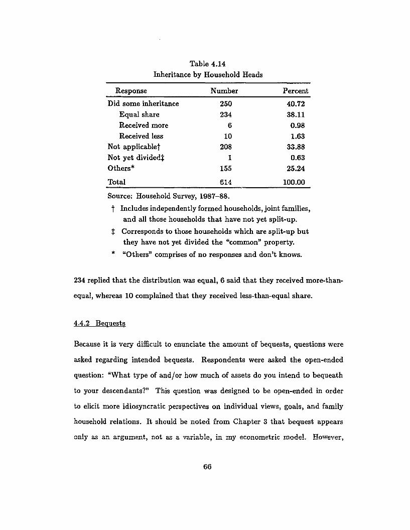
Response
Table 4.14
Inheritance by Household Heads
Number Percent
Did some inheritance
Equal share
Received more
Received less
Not applicable]
Not yet dividedf
Others*Total
250
234
6
10
208
1
155
614
40.72
38.11
0.98
1.63
33.88
0.63
25.24
100.00
Source: Household Survey, 1987-88.
t Includes independently formed households, joint families,
and all those households that have not yet split-up.
:\: Corresponds to those households which are split-up but
they have not yet divided the "common" property.
* "Others" comprises of no responses and don't knows.
234 replied that the distribution was equal, 6 said that they received more-than-
equal, whereas 10 complained that they received less-than-equal share.
4.4.2 Bequests
Because it is very difficult to enunciate the amount of bequests, questions were
asked regarding intended bequests. Respondents were asked the open-ended
question: "What type of and/or how much of assets do you intend to bequeath
to your descendants?" This question was designed to be open-ended in order
to elicit more idiosyncratic perspectives on individual views, goals, and family
household relations. It should be noted from Chapter 3 that bequest appears
only as an argument, not as a variable, in my econometric model. However,
66

the purpose of collecting information on bequests and reporting them here is to
illustrate household heads' views and goals regarding bequests.
Table 4.15
Intended Bequests of Household Heads
Types of Bequests Number Percent
Education 187 30.46
Education+land/house 68 11.08
Whatever is left 47 7.66
Land and house equally 43 7.00
A house each 26 4.23
Medical doctor 14 2.28
Make them independent 14 2.28
Business 13 2.12
Education-l-land-l-house 13 2.12
Higher education 12 1.95
Others] 71 11.56
No response/Don't know 96 15.64
Total 6.64 100.00
Source: Household Survey, 1987-88.
t Includes multiple combinations of all types of responses.
Table 4.15 summarizes the intended bequests of the respondent households.
About 85 percent of all respondents replied that they would like to bequeath
different types of wealth to their children. The remaining 15 percent either did
not respond to the question or just replied, "I do not know." It is remarkable
that none of the household heads wanted not to bequeath anything to his chil
dren. Most of the respondents expected to educate their children rather than
bequeathing money and real estate. The response also varied according to the
occupation of the respondent and the level of his education. Only three heads
67

out of 614 answered that they would like to bequeath a stated amount of money.
(Apparently one of them was not even serious about his answer because he jok-
ingly responded that he would like to bequeath 100 million rupees.)
Descriptive statistics of my household survey were discussed in this chapter.
The following chapter is devoted to projecting future household composition from
the information collected in the survey.
68

CHAPTER 5
PROJECTING FUTURE HOUSEHOLD COMPOSITION
In projecting future household size and composition over the family life-cycle,
we regard the fertility behavior of household head and his spouse and the post-
nuptial living arrangements of their children as the main determinants of future
household size. The fertility behavior of the head and his spouse and the rules
governing living arrangements over the life-cycle are determined from Household
Survey (1987-88) as well as the 1981 census (CBS, Nepal, 1984). The household
survey data have been standardized by assigning appropriate weights to make
the sample data more representative.' The HOMES package is used to gener
ate household composition paths corresponding to different fertility levels of the
surveyed households.
5.1 Structure of Nepali Households
The traditional, as well as the modern, form of the family in Nepal, both rural
and urban, is the extended family consisting of three or more generations. The
extended family system is the result of the influence of tradition and economic
conditions. As far as post-marital residence is concerned, married sons live with
their parents in the same household, and elderly parents live with their son's
family in the same household. Married women go in their husbands' houses.
Nepali is a patrimonial, patriarchal, and patrilocal society. Socially it is not
advisable in Nepal to live in the wife's parental home. The high co-residence
1 A weight variable was calculated from the age distribution of the household populationand the distribution of household size.
69

rate-the proportion of the elderly over 65 who reside with their children or
other relatives-is mainly due to the traditional values accorded to the family
and household in Nepal.
According to the household survey 99.35 percent (610 out of 614) of all
households are family households. The rest are households consisting of primary
individuals (i.e., unrelated individuals). There are no one-person households in
, the sample.
Family households are categorized into three types: (1) intact households,
where both the head and the spouse are present, (2) single-female headed house
holds, and (3) single-male headed households. The second and the third types
of household heads do not have their spouses present.
Table 5.1
Average Number of Household Members
by Their Relationship to the Household Head
Intact Single Female Head Single Male Head
Relationship Number Percent Number Percent Number Percent
Head 1.00 15.40 1.00 13.62 1.00 13.95
Spouse 1.00 15.40
Child 2.94 45.24 2.30 31.25 1.77 24.71
Grandchild 0.54 8.36 2.39 32.59 2.15 29.94
Parent 0.09 1.44 0.06 0.87
Other Relatives 0.66 10.17 1.44 19.64 1.98 27.62
Others 0.26 4.00 0.21 2.90 0.21 2.91
Total 6.49 100.0 7.34 100.00 7.17 100.00
Source: Household Survey, 1987-88.
70

Table 5.1 depicts the size and structure of family households. Single-female
headed households are the largest, exceeding seven members per household. In
tact households have the greatest number of children (approximately three) per
household. Parents and grandchildren comprise less than 10 percent of total
members in intact households. But single-headed households have a significant
proportion of their members in the grandchild category. Other relatives comprise
between two-thirds of a member to about two members per household.
The table also reports that the number of children and grandchildren dom
inates the variation in household size. More than half of family household mem
bers are either children or grandchildren of the household head. The number of
children per family household varies from 1.77 in single-male headed households
to about 3 in intact households. Single-headed households are mostly headed
by widows and widowers; therefore, these household heads are relatively older
than their intact household counterparts. Some of the children of such house
hold heads might have already left their parental household to form their own
household. In addition, such household heads are not at the risk of childbearing."
Therefore, the number of children per single-headed household is smaller than
per intact household. Moreover, some of the heads of single-male headed house
holds are young and never been married. This number is still smaller for such
households. Because single-headed household heads are relatively older than
intact household heads, single-headed households have more grandchildren per
household than intact households.
The number of parents per household is quite low-less than 1.5 percent of
all members are parents. In a society of high co-residence rates, this number
2 Unmarried parenthood is very uncommon in Nepal.
71

seems rather inconsistent. But if we visualize a society with a high fertility rate,
and high prevalence of the extended and joint family systems, these numbers seem
quite logical. The higher the fertility rate the lower will be the probability that
any parent will live with a particular son because there will be more average
number of children per household. The extended family system implies that
multigenerations live in together in the same household; whereas joint family
system means there could be other relatives in that household. Moreover, a
very important factor is the age structure of the population. Not more than 4.0
percent of the population in Nepal is 65 or older." Therefore, these factors lead
to a lower proportion of parents in family households.
Single-female headed households do not have parents as members. There
may be two reasons for this. The first is that such households have not been
included in the sample. The second reason, which I think is also very plausible,
is that single females who have a parent or parent-in-law in the household are
not usually designated as the household head. The parent or the parent-in-law
will be designated as the head.
5.2 The Household Life-cycle
The information presented in the preceding section emphasizes the demographic
characteristics of a household at any point in time; but many decisions of the
household depend on expectations about the household's future composition.
3 According to the 1981 census, the proportion of population that is 65 or older is 3.6percent in Kathmandu, 3.8 percent in Lalitpur, 4.0 percent in Bhaktapur, and 3.2 percentnationwicie (CBS, Nepal, 1984). The survey shows that this proportion is 3.5 percent forKathmandu Valley (Household Survey, 1987-88).
72

Figure 5.1Intact Households
11
10~Q) II.cE 8Q)
~ 7'0l- SQ).cE 5~
Z 4Q)Cl 3eQ) 2~
015-19 25-29 35-39 45-49 55·59 65-69
Age of Spouse
~ Husband and wife ~Chlldren ~ Grandchildren
• Parents o Other relatives o Others
Source: Household Survey, 1987-88.
Households in the family-building stage of their life-cycle base their decisions on
expectations about eventual household size and the future needs of members.
As the household moves along the family life-cycle, its size and composition
changes. Figure 5.1 illustrates how the size and composition of intact households
vary with the age of spouse of the head.' The number of children increases
during the childbearing period and then declines when some children leave their
households, mostly daughters after marriage. Most sons remain in the same
household even after they get married and have their children. Therefore, the
4 Because we have only 501 intact households in our sample the graph has lost some of thesmoothness normal with a larger sample.
73

relative number of grandchildren increases at later stage of the household life-
cycle.
There are significant numbers of other relatives in intact households. These
other relatives include brothers and sisters (including in-laws), nephews and
nieces, cousins, great grandchildren, and multiple wives." The number of other
relatives decreases in households where the head's spouse is in the 30-44 age
group, and then rises again. Such a fall and rise in the number of other relatives
is unlikely, but not altogether impossible. One possible explanation for this de-
cline and incline in the number of other relatives may be because of some of the
brothers and sisters or nephews and nieces or cousins might move out to another
household or form their own. As the household head gets older, the remaining
other relatives might start having their own children, thus, increasing the number
of other relatives again.
5.3 Projecting the Expected Number of Household Members
Estimation of my consumption model requires the expected number of household
members over the life-cycle of the household. Limited information about the
household life-cycle can be obtained from household projections data using a
sample survey. The cross-section data are then interpreted as though they were
time-series data as in cohort analysis. Future membership profiles are estimated
with respect to different fertility scenarios against the age of the marker.6 I have
used the HOMES package to calculate the present value of the expected number
of members in selected age-sex categories."
6 Nine intact household heads in the survey sample have two wives each.6 In intact households, the marker is the head's wife; for other households, the head.7 The foliowing two paragraphs draw hea.vily from Mason (1987b: 1-2).
74
HOMES, A Household Model for Economic and Social Studies, is a demo
graphic model and computer package developed by Mason (1987b) to project the
number and demographic characteristics of households. This model treats the liv-
ing arrangements of other members of the household in a comprehensive fashion.
HOMES calculates different set ... of various "rates" and intergenerational weights
to determine the entire household membership--including the head, the spouse,
children, grandchildren, parents, and other household members-in a fashion
consistent with underlying fertility and mortality trends. Household member
ship is classified by the type of household" and the age of the marker.
HOMES has been developed to deal with the projection of household compo-
sition in the developing country context. It emphasizes the effects of demographic
change on both the number and the composition of households. Therefore, it is
particularly well-suited for application to countries like Nepal, where extended
or multigenerational families are prevalent. This model has been applied to a
number of East and Southeast Asian countries, including Republic of Korea, Tai
wan, Indonesia, Malaysia, Thailand, and the Philippines. However, it has not
yet been applied to any of the South Asian countries.
Data requirements for HOMES consist of population projections that in-
elude age-specific fertility rates, and a recent census or large, representative sur-
vey that includes a household roster with the age, sex, and relationship to the
household head of each household member. For this study, data on population
projections and age-specific fertility rates available from published sources and
data on household membership, including the age, sex, and relationship to the
S HOMES distinguishes households into four types: (1) intact households, (2) single-headedhouseholds, (3) primary-individual households, and (4) one-person households.
75

household head of each household member, available from the household survey
are used.
Some basic assumptions while applying HOMES to constructing curves
should be underlined beforehand. For the present study, I have assumed that:
(1) Household living arrangements as depicted by the 1981 census and the 1987
88 household survey will continue into the future;
(2) Expected survival rate; "an be described by historical survival rates as re-
ported by previous censuses;
(3) In three-generation households, the fertility of the first and second genera-
tions are the same;
(4) Historically observed age-specific fertility rates are the basis for the age
pattern of childbearing to any childbearing level.
Based on these assumptions, HOMES is used to simulate a series of curves
corresponding to selected age-specific fertility rates by using published data and
the 1987-88 household survey data as essential inputs. Selected total fertility
rates and age-specific fertility rates, as shown in Table 5.2, are chosen to cover
all fertility levels of surveyed households.
The person-years of household membership, SNgr, is calculated by
T
SNgT = L e-p(t-T) NgTP(Hat )
t=T(5.1)
where NgT is the expected number of members in each age-sex category" among
surviving households, P{Hat } is the probability that the household will survive
II Four age-sex categories have been distinguished: children 0-9, teenagers 10-19, adultmales 20 and over, and adult females 20 and over.
76

Table 5.2
Age-Specific Fertility Rates
Age Total Fertility Rates
Group 2.0 3.0 4.0 5.0 6.0 7.0
15-19 54.8 63.7 75.8 82.9 72.0 84.0
20-24 132.1 169.4 204.9 240.8 255.7 264.9
25-29 94.8 154.1 201.8 246.9 289.7 326.6
30-34 55.5 95.1 142.5 194.7 254.5 307.8
35-39 33.1 61.4 100.2 145.8 203.9 256.9
40-44 27.1 49.5 64.5 74.7 102.7 130.2
45-49 2.6 6.8 10.3 13.9 21.5 28.9
Source: Calculated from CBS, Nepal, 1984, 1987; and
United Nations, 1985.
from period a to t, and p is the rate of discount assumed to be equal to 0.02 and
0.04.
The calculation of SNg requires the expected number of household members
Ngr in each future period conditional on the household existence and the prob
ability that the household survives to each period. The calculation of these two
components of SNg is discussed below.
5.3.1 Calculating Membership Profiles for Individual Households
The basic approach to calculating the expected number of household members is
based on the life-cycle pattern of household membership that can be characterized
by a family of curves varying with the age of the household marker and the level
of childbearing. Based on the household survey data, age-specific fertility rates as
shown in Table 5.2, and different sets of household membership rates simulated
by using HOMES, HOMES is again applied to generate the numbers that show
77

the person-years of household membership varying with the age of the marker
and the level of childbearing.
Five sets of household membership profiles, one each for four age-sex cate-
gories and the fifth one for total membership, for a household are simulated on
the basis of the fertility behavior of the household. The first four sets of such
profiles are used for estimating the consumption model and the fifth set is used
to illustrate a family of such membership curves (Figure 5.2).
Figure 5.2
Average Members per Household
&1---------------------------,f! 8
1:m 7:e'0 8..1:E 5=ZQ)C) 4l'!!l»
~ 3
__ TFR=2.0
_TFR=5.0Nole: TFR = Total Fertility Rale
35-3& 45-49 55-59
Age of Marker
-e- TFR=3.0 --.to- TFR=4.0
-e-- TFR=6.0 --A- TFR=7.0
85-89
Source: Household Survey, 1987-88.
Figure 5.2 is an example of a family of curves for the total household mem
bership corresponding to different levels of fertility, which have a similar, but
78

unusual, pattern. The curves show a slight decline in the number of household
members for age groups 30-44, but rises very sharply thereafter. The fall is due
to the decline in the average number of "other members" for that age group,
as explained for Figure 5.1. The subsequent rise is because of multigenerational
households thereafter. These membership profiles show that there is a relatively
constant difference in average household size across successive fertility rates. It
means demographic transition in Nepal will not be leading to smaller family size
only at a rather confined "childbearing" interval; rather, it will lead to smaller
family size among households at all ages.
Once a set of household membership profiles is calculated for a particular
category, the following procedure to calculate a family of membership numbers
for an individual household corresponding to different levels of fertility and the
age of the marker is repeated for the remaining categories.
The fertility level of a household is determined by using a combination of the
total number of children and the age of the marker. Then by using the family of
membership curves, the corresponding expected number of household members is
interpolated from adjacent profiles. For the interpolation of expected members,
the following equation is formulated:
(5.2)
where Xi is the calculated number of members for the marker in age group ij Yi
and Zi respectively refer to the number of members in the higher level of fertility
and lower level of fertility for the marker in the ith age group from the standard
profiles; a and (1 - a) are the coefficients representing the weights of Yi and Zi
on Xi, respectively. This implies that Xi is an arithmetic interpolation of Yi and
79

Zi. These coefficients vary from one household to another, but are held constant
within the same household.
The parameter value of ex is estimated for each household using equation
(5.2). If, for example, the fertility level of a household is at point X, which
is somewhere in between level 5 and 6 as shown by Figure 5.2, then solving
equation (5.2) we get the value of ex which is again substituted in the equation to
determine the household membership profile of this household. The values are
then discounted and cumulated for each member from the current age to the end
of family life to determine the expected person-years.
5.3.2 Calculating Household Survival Ratios
Survival ratios are defined in two ages, and hence two time references, the initial
age and date and the terminal age and date. In demography, it is the number of
persons alive in an age group x + k to x + n + k, divided by the number in the
younger age group x to x + n, k years earlier. If the persons alive in these two
cases are represented by the life table population, L, this can be represented as:
This can analogously be applied to determining household survival ratios.
While calculating survival ratios, we use Bayes theorem of conditional probability.
According to the definition of the family life-cycle, family life begins once two
persons marry and form their own household, and ends when they cease to be
designated as household head. Life span of a household will depend on the
probability of the household surviving. Thus, the probability that a household
will survive from age a to age t can be represented as
80

AgeGroup
15-19
20-24
25-29
30-34
35-39
40-44
45-49
50-54
55-59
60-64
65-69
70+
Table 5.3
Household Survival Ratios
FemaleHead
1.0000
0,9753
0.9686
0.9645
0.9597
0.9551
0.9500
0.9427
0.9240
0.8995
0.8529
0.7940
MaleHead
1.0000
0.9815
0.9738
0.9715
0.9674
0.9609
0.9509
0.9375
0.9153
0.8855
0.8374
0.7728
Source: Calculated from CBS, Nepal, 1984.
H(t)P(Hat) = H(a)'
Here H(t) and H(a) denote the total number of households ~hose ages are t and
a respectively.
Similarly, the ratio H(t)jH(a) can further be decomposed and rewritten as
H(t) H(O) H(t)H(a) = H(a) . H(O)'
1P(Hoa) . P(Hot).
(5.3)
This gives us the household survival ratio. Table 5.3 presents the household
survival ratios based on equation (5.3). These values are later substituted in
equation (5.1) to calculate the expected number of household members.
81

Once the survival ratios for households and the expected number of members
in each age-sex category among surviving households are calculated, we can
estimate our consumption model. The estimation of the consumption model is
described in the following chapter.
82

CHAPTER 6
ESTIMATION AND EMPIRICAL FINDINGS
In Chapter 3 we derived the specification of our nonlinear consumption function.
To refresh our memory let us rewrite the expectation function one more time in
abridged form as:
(6.1)
where N e , the current number of equivalent adults, is substituted for (kINl +
k2N2 + k3N3 + k4N4 ) and NL, the lifetime number of equivalent adults, is sub
stituted for (k1SNl + k2SN2 + k3SN3 + k4SN4 + b). Ns, N 2 , N3 , and N 4 are the
numbers of children age 0-9, teenagers 10-19, adult males, and adult females
respectively; SNb SN2 , SN3 , and SN4 are their respective expected numbers but
discounted by the rates of time preference over the life-cycle; C, Y, and A are
respectively the household total expenditures, total income, and household net
assets; and E is the remaining life span of the household.
According to the life-cycle hypothesis, an important factor in determining
household consumption is lifetime resources of the household. In a perfect capital
market, we simply assume that lifetime income is a function of the remaining life
span, net wealth and current income. As discussed in Chapter 3, the first part
of the right hand side of equation (6.1) is the demographic component of the
consumption function, that measures the fraction of lifetime resources consumed
at each household life-cycle stage. Similarly, the second part of the right hand side
of the same equation is the economic component of the consumption function,
83

that measures the fraction of lifetime resources consumed at a given level of
net assets and future income (proxied by the life expectancy of the household
head). Table 6.1 summarizes the mean values of life-cycle household composition,
lifetime equivalent adults, and income profiles.
The age variable in the first column refers to the age of the household head.
Nl, N2' N3' and N 4 in the table are the mean values of the corresponding vari
ables broken down by the age of the head. SNiPj refers to the number of N;
discounted by i percent annually. Two discount rates, 2 percent and 4 percent,
are used for the analytical purposes. The values are negatively related to the
discount rates since they are measured in terms of expected units. The total
number of household members increases with the age of the household head up
to a certain age before it begins to decline. In contrast to the demographic vari
ables, household net assets, current income, and consumption steadily increase
with the age of the household.
Because equation (6.1) is nonlinear in the parameters, not in the variables,
the model cannot be handled in a linear model (Ordinary Least Squares) frame
work. To estimate the unknown parameters, an objective function is specified
and an optimal value of the unknown coefficient vector is computed as the es
timate. However, as in the Ordinary Least Squares method, we still have to
estimate the coefficient parameters that minimize the sum of squared errors of
a nonlinear statistical model. But the problems with nonlinear models are that
a system of nonlinear normal equations has to be solved to find the solution of
the optimization problem, and a closed form expression of the resulting estima
tor cannot usually be given. Therefore, its normal equations cannot usually be
solved analytically, and there may be multiple solutions not all corresponding
84

Table 6.1
Mean Values of Demographic and Economic Variables
Nl N2 N3 N4 SN1P2 SN2P2 SN3P2 SN4P2 SN1P4 SN2P4 SN3P4 SN4P4 A Y C
0.500 1.167 1.000 0.333 5.720 6.162 12.191 6.771 5.180 5.594 11.113 6.030 241202 65740 281521.300 0.675 1.400 1.100 5.103 8.155 11.249 9.925 4.627 7.341 9.926 8.763 418900 62689 434551.718 0.634 1.408 1.099 5.639 8.463 12.069 10.193 5.151 7.730 10.783 9.121 404588 58108 482921.652 1.797 1.290 1.391 6.650 8.490 11.797 10.066 6.103 7.893 10.679 9.133 701655 70529 611190.857 2.312 1.234 1.221 5.778 7.407 11.594 9.788 5.344 6.963 10.645 8.994 785979 69118 600000.569 2.264 1.750 1.458 5.205 6.805 12.903 10.639 4.880 6.445 12.023 9.909 839288 74632 581811.095 2.027 2.311 2.041 5.088 5.672 12.705 11.441 4.846 5.410 12.002 10.805 1233194 81992 662311.385 1.462 2.646 2.492 4.875 5.079 11.413 11.081 4.695 4.871 10.915 10.595 1322581 102718 700461.619 1.524 3.310 2.667 5.741 5.525 12.821 11.064 5.587 5.34'5 12.401 10.699 1634333 95025 766121.769 1.205 2.462 2.462 4.347 4.664 10.129 9.209 4.280 4.557 9.898 9.004 1064657 70065 589932.000 1.500 2.944 2.500 4.528 5.586 10.144 8.615 4.498 5.520 10.029 8.518 871220 75636 664331.075 1.700 2.625 2.425 2.609 4.126 6.371 5.886 2.609 4.126 6.371 5.886 1574433 160313 76727
AGE
15-1920-2425-2930-3435-3940-4445-4950-5455-5960-6465-70
70 +00C11====================================================
Noto: AGE rofors to tho ago of the housohold markor;
N1 rofors to tho number 01children aged 0-9;
N2 relers to the number of teenagers aged 10-19;
N3 relers to the number of adult males (aged 20 and above);
N4 relers to the number of adult females (aged 20 and above);
SNiPj relers to the expected number of Ni discounted by j percent annually;
A,Y and C denote total assets, Income and consumption respectively.
to the global minimum of the sum of squares functions. Maximum likelihood
method, whose great advantage is that under a broad set of conditions, parame
ter estimators are both consistent and (for large samples) asymptotically efficient,
is employed to estimate the model as specified by equation (6.1).
6.1 Estimation Procedure
Many econometric textbooks (for example, Pindyck and Rubinfeld, 1991; In
triligator, 1978) have dealt with the discussion of nonlinear estimation. A more
rigorous treatment of nonlinear estimation can be found in Judge et al. (1985,
1988) which has mainly been followed for this analysis.
If we specify our model in matrix notations as
y(t) = f[X(t),,8] + €(t) (6.2)
where y is a (T x 1) vector of observed sample values of the dependent variable;
X is a (T x K) matrix of known values of the explanatory variables;,8 is a
(K x 1) vector of unknown coefficients; and € is an unobservable (T x 1) vector
of real random variables with mean zero and variance u 2 •
To apply the maximum likelihood method for estimation we assume that
all the required derivatives of f (*) exist and are continuous, and the error terms
€ are independent, identically and normally distributed (i.i.d.) with mean zero
and variance u 2 • Mathematically it can be written as
86

and
E(E~Ej) to, for it i.(6.3)
Based on assumption (6.3), the parameter vector 13 is estimated by maxi
mizing the likelihood function
2 1 {_ (Y-IIX,iJ)I' ~Y-:-I(X,llll}1(13.o ) = T e 20'
(2IIu2)"2
1 {~}- -----:x.=-e - 20'2
(2IIu2) 2
(6.4)
where S(f3) = [Y - f(X, ,8)]'[Y - f(X, 13)] is the sum of the square of error terms.
Maximizing this function is equivalent to minimizing
(6.5)
Equation (6.4) is maximum when S(f3) is minimum.'
To estimate the parameter vector 13 which minimizes equation (6.5), which
in turn maximizes our likelihood function, we will use a three-step procedure
known as iterative minimization procedure, as described below.
1. A set of estimates, for example 130 = (f3oll 1302, .•. , f30k) , is initially assumed,
and the corresponding value of the likelihood function, as represented by
equation (6.4), and the sum of squared errors, SJ~), are calculated.
2. The preceding step is repeated with a different set of ,8 estimates with (,80 +
D.) . If S (,80 + D.) < S (,8) then the revised estimate of 13 is set equal to
1 This follows that maximum likelihood estimators of the parameters /3 are identically equalto the least squares estimators.
87

(,80+.6.). Otherwise a A, where 0 < A < 1, is found such that 8(,8+.6. x A) <
8(,80), and ,81 is set equal to (,8 + .6. x A), provided that such a A exists.
According to the gradient method, A and .6. refer respectively to a step
direction and step length, both of which are used to obtain the minimum
value of the sum of squared residuals.
3. Steps 1 and 2 are repeated and the iterative method is continued until the
values of ,8 on successive iterations stabilize. This can be measured by the
size of each parameter increment relative to the previous parameter value,
which is the basis for one of the common criteria used to declare convergence.
When the parameter vector is estimated we can also estimate the variance-
covariance matrix. On the assumption laid down on equation (6.2), the asymp
totic variance-covariance matrix of Pis estimated by
V(P) = { S~) } x {~z,z,} -1 (6.6)
where Zi = 8f(,8i,Xi)/8(Pi) are evaluated at ,8; and N is the number of obser-
vations.
The SHAZAM computer package (White et al., 1990) has been used to
estimate the nonlinear parameter vector." Nonlinear estimation in SHAZAM
applies the gradient method (also known as the quasi-Newton method) as its
algorithm to obtain estimates that maximize the likelihood function. Various
sets of starting values have been tried to confirm that a global minimum has
probably been achieved.
2 The LimDep, SAS, and SHAZAM programs were used to test their relative efficiency[in terms of time) for estlmatlng nonlinear parameter vector. The experiment showedSHAZAM to be more efficient than any of the other two programs. Hence, the SHAZAMprogram has been used throughout the analysis.
88

6.2 Statistical Tests
Only asymptotic properties of the parameter estimators for nonlinear models
are generally available. Therefore the usual interval estimators or confidence
regions are also only approximately or asymptotically correct and justifiable.
Inferences are drawn by estimating and testing the coefficient parameters, where
the estimators have variance-covariance matrix as specified by equation (6.6).
6.2.1 Testing Hypotheses
In order to test the hypothesis
Ho : 13; = c against H a : 13; f. c(6.7)
where 13 is a vector of k parameters and c is a vector of k constants, the asymptotic
normality of the maximum likelihood is used. Null hypotheses are tested at a
prespecified level of significance.
Various methods of hypothesis testing, such as the Wald Test, Lagrange
Multiplier Test, and Likelihood Ratio Test, have been suggested. In this study,
however, I use the likelihood ratio test to test the null hypothesis (6.7). This
test statistically compares constrained estimators with the unconstrained ones.
If, for example, f3uRand 13R are the respective maximum likelihood estimators
of unconstrained and constrained f3's when the null hypothesis (6.7) is imposed,
then the null hypothesis is rejected if
A = 2 [lnL(f3uR) -lnL(f3R)]
89
(6.8)

exceeds X2 (J, a} for a prespecified significance level a with J degrees of freedom."
The degrees of freedom are determined by the number of additional restrictions
imposed in the restricted model as compared to the unrestricted model.
6.2.2 Testing the Model's Specification
The objective of testing a model's specification is to examine the validity of the
model and the variables therein. In our analysis testing the model's specification
is to investigate whether demographic variables are significant determinants of
household consumption as specified by equation (6.1).
To answer this question we compare the life-cycle consumption model (6.1)
with a simple model without demographic variables. The modified specification
is written as
In (~) = ko In (~:) + In[ks (¢ } + k6El (6.9)
where ko reflects the validity of the specified life cycle consumption model." If
ko is positive and statistically significant then we can infer that the demographic
3 The Lagrange Multiplier test is based only on the restricted maximum likelihood (ML)estimator, while the Wald test is based only on the unrestricted ML estimator. Thelikelihood ratio test uses both the restricted and unrestricted estimators as shown by(6.8). Because it requires both restricted and unrestricted estimates, the likelihood ratiotest is likely to be computationally more demanding than the Wald test or the LagrangeMultiplier test.
4 An immediate query may arise here that whatever is good for the goose should be good forthe gander, indicating that if we are to test the validity of demographic variables we shouldalso simultaneously test the validity of economic variables in similar fashion. Therefore, Iset up an alternate function by respecifying the model as
However, such a function could not be estimated because of continuous error messagesfrom the computer program.
90
variables influence household consumption. If not, household consumption is
solely determined by assets and income under the linear specification.
6.3 Estimated Functions and Discussion
Table 6.2 presents parameter estimates and their asymptotic standard errors for
four versions of the life-cycle consumption model. The estimates show that all
variables except the ratio of net assets to current income and the b parameter
are significantly different from zero.
First, we assume that the demographic variables do affect household con
sumption; thus, ko is set to unity," Second, two different versions of the full
model with rate of time preference equal to 0.02 and 0.04 have been estimated.
Third, since the ratio of net assets to current income does not seem to be a
significant variable in either of these two models, we constrain the parameter
estimate for this variable equal to ka to estimate Models 3 and 4.
All of the models show that kg is constrained to equal 1. By imposing this
condition as the standard adult scale for adult male, the estimates of kI, k2 , kg,
and k4 are interpreted in terms of relative equivalent adult males.
Recall that the parameters have the following interpretations:
k1 is the relative weight of children age 0-9,
k2 is the relative weight of teenagers age 10-19,
kg is set equal to 1, the standard adult scale,
k4 is the relative weight of adult females,
ks is the effect of the net assets-current income ratio on consumption,
6 This assumption will be tested later.
91

Table 6.2
Parameter Estimates for Different Models
Modell Model 2 Model 3 Model 4Parameter p=2% p=4% p=2% p=4%
b 58.785 49.723 0.0000* 0.0000*(45.868) (40.787)
k1 0.9457 0.9379 2.7100 2.5439(0.2999) (0.2918) (1.0368) (0.9118)
k2 1.4665 1.4604 3.3619 3.i053(0.3776) (0.3621) (1.2550) (1.0533)
k3 1.0000* 1.0000* 1.0000* 1.0000*
k4 0.9222 0.9233 0.5132 0.5494(0.4383) (0.4371) (0.6160) (0.5714)
ks 0.1377 0.1204 0.0667<> 0.0643<>(0.0897) (0.0798) (0.0027) (0.0025)
k6 0.4194 0.3656 0.0667<> 0.0643<>(0.2123) (0.1900) (0.0027) (0.0025)
q2 0.8104 0.8105 0.9520 0.9395
LLF -805.38 -805.44 -854.74 -850.69
SSE 496.79 496.89 583.60 575.94
N 613 613 613 613
Note: Numbers in parentheses are asymptotic standard errors.
LLF, SSE and N respectively denote log-likelihood function,
sum of squared residuals and number of observations.* An asterisk indicates that the parameter is constrained to equal
the shown value.<> A diamond indicates that ks and k6 are constrained to be equal.
92

k6 is the growth rate cf future income measured as the effect of head's life
expectancy on consumption,
b is the number of equivalent adult years of consumption that an average
family leaves as bequests.
Let us take a look at Table 6.2 where Modell and Model 2 represent the full
model. The estimated coefficients (equivalent adult units) for children, teenagers
and adult females are respectively 0.94, 1.46, and 0.92, assuming that the equiva
lent adult unit of an adult male is one. These large values of the equivalent units
suggest that children have a stronger effect in Nepal than typically found in the
literature. However, given the asymptotic standard errors, we cannot reject the
hypotheses that kI, k2 , k4 = 1. Hence the values of 0.92 or more cannot be
distinguished from unity. Because this study is limited by a small sample size,
no firm conclusions could be drawn.
Two factors may account for the teenage coefficients. First, the dependent
variable is ClY; not c. Thus, while children may account for less consumption
than adults, they bring in no income, which causes their presence in the household
to yield a higher C / Y than for an adult male. Second, even in absolute terms,
Nepali families living in Kathmandu with school children may well spend more on
them than on a typical adult because primary to high schooling is very expensive.
Though the public schools are free until third grade and nominal tuitions are
charged thereafter up to high school, private schools are much more expensive
than colleges or the university. To keep up with other households, most of the
parents would like to enroll their children in private schools. Therefore, heavy
outlay for tuitions, fees, and school supplies make teenagers more expensive to
93

raise them than anybody else. However, given the asymptotic standard errors,
we cannot reject the hypotheses that k2 = 1.
The estimated equivalent adults from Table 6.2 are individually not signifi
cantly different from one, implying that age and sex do not matter in determining
household consumption. To test this hypothesis, I constrained kll k2 , kg, and
k4 to be equal to 1 in the restricted model and compare the results with those
of the unrestricted model. 6 Table 6.3 compares the parameter results of the two
models.
From the likelihood ratio test we cannot reject the null hypothesis that
the equivalent adult units of household members are not different from unity at
the 5 percent level of significance. The demographic variables are jointly, but
not individually, significant. In other words, household consumption depends
on household size but there is no evidence that it varies with age and sex of
household members. However the null hypothesis is rejected at the 10 percent
level of significance.
The positive coefficients for the ratio of net assets to current income on
consumption show that consumption ratio increases with net assets. However,
these coefficients are not statistically significant. From hypothesis testing we
cannot reject the null hypothesis that k 5 is equal to zero at the 0.05 level of
significance. This could have occurred for two reasons. First, the net assets may
not be an adequate variable for differentiating income from wealth. Second, there
could be some error in the measurement of the net assets.
The growth rate of current income is captured by k6 • It measures the effect of
the household head's life expectancy (a proxy for future income) on the household
6 Model i in Ta.ble 6.2.
94
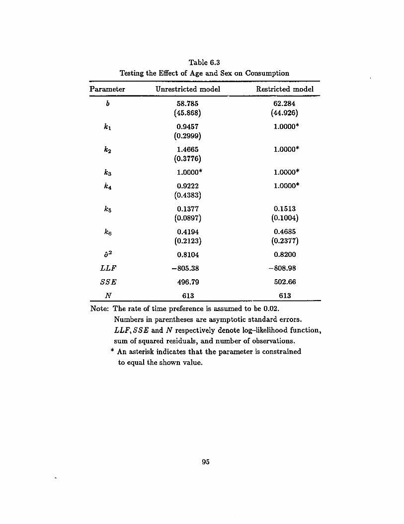
Table 6.3
Testing the Effect of Age and Sex on Consumption
Parameter Unrestricted model Restricted model
b 58.785 62.284(45.868) (44.926)
k1 0.9457 1.0000*(0.2999)
k2 1.4665 1.0000*(0.3776)
kg 1.0000* 1.0000*
k4 0.9222 1.0000*(0.4383)
ks 0.1377 0.1513(0.0897) (0.1004)
k6 0.4194 0.4685(0.2123) (0.2377)
q2 0.8104 0.8200
LLF -805.38 -808.98
SSE 496.79 502.66
N 613 613
Note: The rate of time preference is assumed to be 0.02.
Numbers in parentheses are asymptotic standard errors.
LLF~SSE and N respectively denote log-likelihood function,sum of squared residuals, and number of observations.
* An asterisk indicates that the parameter is constrained
to equal the shown value.
95

consumption ratio. On average, a unit increase in the head's life expectancy (a
proxy for lifetime income relative to current income) will increase a household's
consumption ratio by 0.40. Its value is negatively related to the discount rates
since it is measured in terms of expected units.
Models 1 and 2 in Table 6.2 show that the estimated values of b are about
59 and 50 respectively. b can be interpreted as the number of equivalent years
of consumption that an average family leaves (or plans to leave) as bequests. As
explained during my model development, b is a parameter of bequest elasticity.
However, we do not see that b =f:. 0 because this value is not significantly different
from zero, indicating that households seem to be consuming all of their resources
during their lifetime. In other words, there is no evidence for strong bequest
motives.
According to the 1981 census, the life expectancies at birth of a Nepali male
and a Nepali female are 50.88 and 48.10 years, respectively (CBS, Nepal, 1987:
352-353). Ignoring some minor details, these values of b, 59 and 50, denote almost
the whole life span of a person throughout his life-cycle. Despite such large values
of b, it is statistically insignificant because of large values of its standard errors.
These large values of standard errors could have occurred for one or more of the
following reasons, such as the choice of wrong discount rates, underconsumption
by households, the heads are not certain about their life expectancy and want to
save more for future.
Models 3 and 4 in Table 6.2 show the parameter estimates when we constrain
the parameter estimates of the nondemographic variables, e.g., net assets/income
96

ratio and head's life expectancy, to be equal.7 The rationale for imposing this
constraint is that, because we assumed in Chapter 3 that 9 (the growth rate of in
come) is small, the hypothesis that 9 = 0 is tested by this constraint model. These
models, however, show very different results as compared to the results shown
by preceding models. The coefficients for children and teenagers are greater here
than 1 while the coefficients for adult females are less than 1. In these models
all the coefficients except those for adult females are found to be significantly
different from zero at the 5 percent level. However, none of these estimates for
demographic variables are significantly different from 1 (except for teenagers in
Model 4).
In section 6.2.2 I brought up the issue of testing the model specification. I
now discuss the results estimated from the specification given by equation (6.9).
As assumed, ko reflects the validity of incorporating demographic variables in
the household consumption function specified by the original nonlinear equation
(3.24). The coefficient estimates and their standard errors for equation (6.9) are
shown in Table 6.4. The table shows that all equivalent adult units (excluding
the adult male scale which is the reference scale) are greater than 1. But the
test shows that none of them is significantly different from 1. The values of R2
and the log-likelihood function are higher for the unrestricted model than for
the restricted model." Using the likelihood ratio test, one can infer that the age
7 Note that ko is also constrained to equal zero in Models 3 and 4. These models could notbe estimated with an unconstrained value of ke- Various sets of starting values were tried,but any such attempt was fruitless until I constrained ko equal to zero because otherwisethe results showed very wild values. In addition, Models 1 and 2 showed that b = 0 cannotbe rejected.
8 The restricted model here completely ignores demographic variables, treating all equivalent adult scales equal zero. Therefore, this model represents the original life-cycle modelwhere consumption depends only upon household assets and life expectancy. Alternativespecifications such as one with an intercept term, and another with an intercept and a multiplicative terms were also estimated. But the results showed that the present specificationwould be the "best" fit of all.
97

Table 6.4
Testing the Model Specification
Parameter Unrestricted model
ko 0.3833(0.0526)
b -3.5156(1.7109)
k1 1.2929(0.3089)
k2 1.7594(0.4902)
k3 1.0000*
k4 1.1798(0.6079)
ks 0.0184(0.0032)
ka 0.0604(0.0069)
&2 0.6895
LLF -755.86
SSE 422.67
N 613
Restricted model
0.0000*
0.0178(0.0019)
0.0324(0.0015)
0.7617
-786.39
466.93
613
Note: The rate of time preference is assumed to be 0.02.
Numbers in parentheses are asymptotic standard errors.
LLF, SSE and N respectively denote log-likelihood function,
sum of squared residuals, and number of observations.
* An asterisk indicates that the parameter is constrained
to equal the shown value.
98

and sex composition do have a significant effect on household consumption at
the 0.05 confidence region.
One can clearly draw two major inferences from this table. First, ko is sig
nificantly different from zero indicating that exclusion of demographic variables
would misspecify our model. The hypothesis that ko is equal to one as specified
by our general model is also rejected because ko is significantly different from 1.0
That ko is less than 1 implies that the relationship between demographic vari
ables and household consumption is not that simple as specified by the general
model. It means the general model is assigning inappropriate weight to the de
mographic component of the consumption model. This model shows that the role
of demographic variables is overemphasized in the general model as compared to
the economic component. Second, the parameter b is found to be significantly
different from zero. As explained earlier, b is a bequest parameter. Therefore,
if we allow ko to vary, we reject b = 0, indicating that bequests also plays a
significant role in explaining the household consumption patterns.
The inferences drawn so far confirm that demographic factors positively
affect the household consumption ratio. Similarly, the results also show that life
time income profile, which has been proxied by the household net assets and the
life expectancy of the head, has a positive effect on the household consumption
ratio. Nevertheless, the model does not tell us anything about the sensitivity of
the demographic factors to the variation in equivalent adult parameters.
To test the sensitivity of the demographic factors to the variation in equiv-
alent adult parameters, one can generate various sets of numbers that show the
o A slightly variant specification for equation (6.9) was also estimated by treating ko asan intercept rather than an multiplicative factor. The results, however, showed that thecurrent specifica.tion would yield a "better" fit than the alternate one.
99
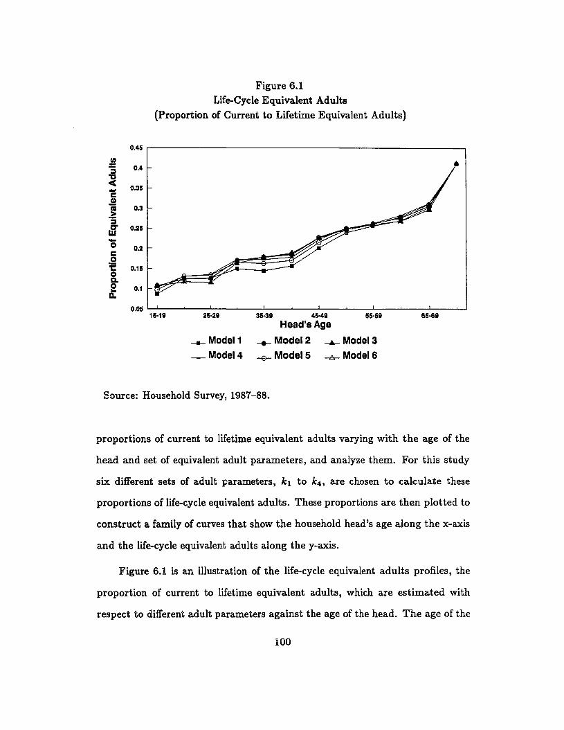
Figure 6.1Life-Cycle Equivalent Adults
(Proportion of Current to Lifetime Equivalent Adults)
0.45
JS0.4="c(
0.35-CQ)
'i 0.3.~
=~ 0.25-0 0.2C01: 0.150a.0 0.1..a.
0.0515·19 25·29
__ Model 1
_Model4
35-38 45-49 55·58 65-69Head's Age
___Model 2 ---.6r- Model 3
-B- Model 5 -A- Model 6
Source: Household Survey, 1987-88.
proportions of current to lifetime equivalent adults varying with the age of the
head and set of equivalent adult parameters, and analyze them. For this study
six different sets of adult parameters, k1 to k4 , are chosen to calculate these
proportions of life-cycle equivalent adults. These proportions are then plotted to
construct a family of curves that show the household head's age along the x-axis
and the life-cycle equivalent adults along the y-axis.
Figure 6.1 is an illustration of the life-cycle equivalent adults profiles, the
proportion of current to lifetime equivalent adults, which are estimated with
respect to different adult parameters against the age of the head. The age of the
100

head and the values of demographic variables are taken from Table 6.1. If we
denote the values of k,'s as a vector, then Modell through Model 6 in Figure 6.1
denote the equivalent adult vectors [0.5,0.5, 1.0, 1.0], [0.9, 1.5, 1.0,0.9], [0.5, 1.4,
1.0) 0.9], [1.2, 1.3,1.0,0.9], [1.0,1.0,1.0,1.0], and [0.9, 1.4, 1.0,0.9] respectively.
The figure shows that demographic factors are very insensitive to the varia
tion in equivalent adult parameters. The values of the equivalent adult parame
ters cover a wide range of values. However, the graph shows that these simulated
curves have little variation. This could be because of Nepal's demographic char
acteristics (a young population and high fertility), living arrangements, and/or
the relatively small sample size used in this study. The finding that demographic
factors are be very insensitive to the variation in equivalent adult parameters
could have resulted to infer from the alternative specification of our consumption
model that the general model overemphasizes the role of demographic variables
in explaining the household consumption behavior.
6.4 Summary
The basic concept underlying the life-cycle model is that a household bases its
current consumption decisions upon lifetime expectations about income and fam
ily composition. The model developed during the course of this study seems to
be quite appropriate for examining the effect of demographic variables. Results
here show that a model with classified age-sex categories explains the effect of
demographic variables because the estimated coefficients are significantly differ
ent from zero. Statistical testing of the model has produced some evidence that
demographic variables in addition to lifetime resources do influence household
consumption decisions.
101

CHAPTER '1
CONCLUSIONS AND POLICY IMPLICATIONS
The empirical analysis based on the theoretical model developed for this study
shows the extent to which household composition affects the consumption be
havior of households. A distinction between household size ?..nd household com
position is made. A life-cycle path of household composition is formulated by
projecting the lifetime membership profiles of households. HOMES has been used
to construct these household membership profiles. The empirical results confirm
the hypotheses that the magnitude and direction of demographic variables influ
ence household consumption behavior. The following section reviews the major
results and the policy implications that can be drawn from these findings. Fi
nally, some of the limitations of the present study are identified and suggestions
regarding future research are outlined.
'1.1 Major Results and Policy Implications
This study extended the life-cycle consumption model (Modigliani and Brum
berg, 1954; Fisher, 1956; Modigliani and Ando, 1957; Ando and Modigliani,
1963) to account for the effects of demographic variables (changing household
composition) on household consumption behavior. Primary data collected from
a field survey during 1987-88 in Kathmandu (Household Survey, 1987-88) and
the 1981 census data of Nepal (CBS, Nepal, 1984) have been used to estimate fu
ture household membership profiles and the consumption function. A nonlinear
102
regression analysis method has been applied to estimate the parameter coeffi
cients. Hypotheses have been tested to draw statistical inferences regarding the
estimated parameter coefficients.
The findings provide ample evidence that changing household composition
does significantly affect household consumption patterns. A restricted model,
where demographic variables do not have any effect on consumption patterns is
also estimated. The log-likelihood ratio test regarding the comparison of the
restricted model and the unrestricted model indicates that the restricted model
should be rejected because demographic variables do have a significant effect on
household consumption.
In addition, equivalence scales have been estimated to measure the weight of
the age-sex structure of household members on household consumption. Adult
males, males age 20 or above, have been standardized to a scale of 1 and cor
responding scales for other age-sex categories have been estimated. The results
show that the estimate coefficients for teenagers are greater than 1, and the
coefficients for other age-sex categories are close to 1. These greater-than-one
coefficients for teenagers occur for mainly of two reasons. First, teenagers bring
in no income into the household. Therefore, their presence in the household
causes a higher C/Y than for an adult male. Second, education in Kathmandu,
particularly primary to high school, is very expensive. Heavy outlays for tuitions,
fees, and school supplies makes teenagers more expensive to raise than anybody
else. However, we cannot reject the hypotheses that equivalent adult units are all
equal to 1. The value of 0.92 for adult females or more cannot be distinguished
from unity.
103

Testing our general model's specification to examine the validity of the model
and variables therein show that the relationship between demographic variables
and consumption is not linear as specified by the model. In addition, the param
eter b is found to be significantly different from zero. It should be noted that
b is a parameter of bequest elasticity. Therefore, if we allow the coefficient of
demographic effect to vary, we reject b = 0, indicating that households do not
seem to be consuming all of their resources during their lifetime.
It should be noted that besides demonstrating the importance of demo
graphic variables, analysis of consumption data provides additional support for
the inclusion of population growth as a major factor affecting household con
sumption patterns. Any change in fertility behavior and/or mortality will affect
population growth in one way or another. For example, holding mortality and
migration constant, a sudden decline in the fertility level would decrease the na
tional population growth rate, and there will be fewer-than-expected members
in existing households as well, especially in lower age categories. One policy
implication that can be drawn from this is that decline in fertility lowers the
consumption propensity of a household. But if we look at the expenditures on
education this might not always be true. Lower fertility increases expenditures
on children's education implying a demand for better quality children.
In this study a family of household membership curves with respect to dif
ferent fertility levels is also shown. Based on these curves, a life-cycle household
consumption function can be derived for different time periods and discount
rates. The evidence suggests that the addition of a member in the household
increases the amount of household consumption.
104

'1.2 Limitations of the Study and Suggestions for Future Research
Despite the conclusions drawn from the findings and interpretations of our results
during the course of this study, this analysis is not perfect and has its own
lim.itations. This study also explores some prospects for future research related
to this field. Some of the limitations and suggestions for future research are:
First, the use of a sample household survey taken only from Kathmandu
Valley is not representative of the national population. Thus, these results can
not be generalized to the national level. These sample data are standardized
to the Kathmandu population distribution so as to make them reflect the na
tional demographic structure. Though it may reflect the national demographic
distribution, household composition, and living arrangements, it does not reflect
nationwide consumption patterns. About 93 percent of the Nepali population
lives in rural areas. But these sample data are taken from Kathmandu. The
living arrangements in Kathmandu do not necessarily reflect the living arrange
ments in rural Nepal.
Nonetheless, even though there are some differences in the living arrange
ments between rural and urban areas, they still have many things in common.
The social and cultural values that guide and order living arrangements are the
same throughout the country. They may not be the exactly same from place to
place, but if they differ, it is only insignificantly.
Second, the model derived in this study is a long-run comparative-static one.
A short-run dynamic model of household composition and consumption behavior
may be needed when fertility levels and the social norm about nuclear households
are changing rapidly.
105

Third, this study looks broadly into the relationship between household com
position and the aggregate household consumption propensity. There are other
macroeconomic variables that should be taken into account in future research.
For instance, parents may perceive differently the effects of schooling of daughters
and sons. The education of a son, who will stay with his parents in their old age,
may influence consumption differently than that of a daughter, who leaves after
her marriage. In addition to the differences in sex, whether people live in ur
ban or rural areas may affect the aggregate consumption propensity. The larger
the proportion of people living in urban areas, the more important the nuclear
family might be. The breakdown of the extended family may lead to a decline
in the importance of investment in the schooling of children. Consequently, the
consumption propensity changes.
Fourth, in rural areas, it is difficult to measure household income and ex
penditures because most of their income is in kind and the economy is poorly
monetized. Rural people use exchange labor as well as their own household labor,
which is sometimes intermittent, and sometimes dawn to dusk. The monetary
valuation of children's contribution to household income and older generations'
contribution to household income, management, and child care are also difficult
to calculate and measure. We can only approximate them.
A very important topic for future research from this survey data would be an
analysis of consumer expenditures based on the extended consumer expenditure
approach developed by Deaton (1982) and applied by many other researchers.'
Analysis using this data set could lead to production of a research paper with
interesting results.
1 See, for example, Deaton and Muellbauer (1986).
106

The HOMES model of the household sector of the economy could be used
to assess how general economic conditions and demographic change will affect
various dimensions of the household sector and, in turn, to determine how key as
pects of the general economy will be affected by changes in the household sector.
The household sector can be taken to include (1) the supply of labor, (2) school
enrollment and educational attainment, (3) household saving, (4) household ex
penditure, (5) housing demand, (6) health-care utilization, and (7) contraceptive
use.
There will be a population census of Nepal in June 1991. An extension of
this study to the forthcoming census could be a timely and appropriate topic
for future research. These 1991 census data can be used to formulate the future
development planning of the country. HOMES can be applied to project the size
and composition of Nepali households and population, so that the government
formed under a new political system and spirit could utilize the information
to layout its future development plans based on projections on demand for
housing, the labor force situation, and the national saving rate. My model is
a microeconomic model with macroeconomic implications and could contribute
concrete macroeconomic policy guidance to the government.
'1.3 Conclusions
Household fertility behavior and its expenditure pattern are important in eco
nomic development because capital and population are major factors contribut
ing to economic growth. The theory developed so far provides a framework to
analyze the relationship between changing household composition and its con
sumption behavior. In making decisions of how much to spend on household
107

consumption and how much to save (or dissave), households base their decisions
on two objectives: (1) to maximize the utility from household consumption, and
(2) to achieve a desired distribution of wealth. In addition, the size and compo
sition of a household may be an important factor in determining household time
preference and tastes, which, in turn, affect the consumption propensity.
The importance of household composition in increasing economic growth
has been shown in many studies. This study shows the life-cycle consumption of
Kathmandu households in a changing household composition pattern. HOMES,
A Household Model for Economic and Social studies, is applied to project a fam
ily of curves projecting future household membership. This information is used
to estimate a life-cycle consumption function, and equivalence scales have been
estimated to measure the effect of household age-sex composition on consump
tion. The findings show the importance of demographic variables in estimating
consumption functions. It is seen that teenagers consume more than adult males,
but the difference is statistically insignificant. The difference between adult male
and adult female scaling factors are also not significantly different.
The effect of demographic variables is not only through the existing age-sex
composition of the household but also through the expected lifetime composition.
The findings suggest a greater role of household composition in consumption,
which in turn affects saving and economic development.
108

APPENDIX
QUESTIONNAmE
Namaste!*
How are you? My name is . I came hereto see you and ask a few questions about the composition and the incomeexpenditure pattern of your household. This is a research study on "Life-CycleAnalysis of Household Composition and Family Consumption Behavior" beingconducted by Nav Raj Kanel for his Ph.D. in Economics. I know you are verybusy, but I would appreciate it very much if you could help us by answering thequestions asked in this questionnaire.
We would like to assure you that this work is not associated with any government office or any organization, and your answers to these questions will bekept confidential and used for research purposes only.
Thank you.
Interviewer (Narne):
Date:
Time (Interview started):
Time (Interview completed):
* Namate is a Nepali greeting word.
109

Household # :A. HOUSEHOLD ROSTER
[Note: Use extra sheet if the household size is more than six.]
AI. Could you please supply the following information of all the people wholive here and eat together in this household?(Please write the name of the head at column 1.)
Person No.
Name
Sex
Age
Date of birth
Occupation
Relationship to thehead of the household
Ethnicity:
1 2 3 4 5 6
What language is most commonly spoken in this household?
(For age 6 and above only)
A2. What is the highest level(year) of schoolinghe/she has completed?
Currently enrolled at school?
If only literate,please specify so.
A3. What is the marital status ofeach of the household members?
(a) single
(b) married(c) widowed(d) divorced
(e) separatedWhat was the age at marriage?
110

Person No. 1 2 3 4 5 6
A4. How long was he/she presentin this household duringthe past 12 months?
(a) less than six months
(b) about six months
(c) more than six months
If not 12 months, purpose of absence:
AS. How long has he/she livedcontinuously in his household?(Please specify the time period)
B. FERTILITY INFORMATION
* Note: Ask to ali ever-married women.
Person No. 1 2 3
Name of the woman
Number of live births
Bl. How many living sonsand daughters do you have?(Identify with person number)
B2. How many of your sons anddaughters live elsewhereother than this household?
B3. At what age did they leavethis household?
B4. Do you expect to haveany more children?
(1) No (2) Yes (3) Uncertain
If Yes, how many additionalchildren do you think youare likely to have?
111

Person No. 1 2 3 4 5 6
B5. For a couple in your economiccircumstances, what is thebest number of living sons andand daughters?
B6a. Do you know of any methodscouples use to keep from havingmore children than they want?
() No () Yes
b. Are you or your spouse usingany such method(s)?
() No () Yes
H Yes, which method(s)?
c. H No, do you plan toone in the future?
() No () Yes
H Yes, which method(s)?
C. ASSETS AND INCOME (Nepali Rupees as the monetary unit)Respondent's Narne:Respondent's Person Number (From the household Roster):Residence
Cl. Is this house owned by someone who lives here in this household, or is itrented, or you live here free?
(1) Own (2) Rent (3) Free (4) Other (please specify):
H rented, what is the rent per month?
Otherwise, how much would have it cost you to pay rent for this housing?Rents per month:
C2. How many rooms do you have in this household for the exclusive use ofthis household? Number of rooms:
C3. Does this household have electricity? () No ( ) Yes
112

Household Items
C4. How many, if any, of the following items do you have in this household?
Items
(a) electric fan
(b) electric iron
(c) TV
(d) refrigerator
(e) radio
(f) car
(g) telephone
(h) wrist watch
(i) bicycle
OJ motorcycle
(k) ...(1) ...(m) ...
Number Value (or cost anddate ofpurchase)
BusinessUse?
Land
C5. Does this household own any agricultural land?
( ) No ( ) Yes
If Yes, total land area (in Ropani):
Please give the description of your land on the following table.
Plot Size Type ofland
Rented orprivate
Productionper year
Principal Netearnings for thelast 12 months
C6. Do you use any power equipment (tractor etc.] on your farm?
( ) No () Yes
If Yes, type of equipment(s):
Is this your own equipment, or borrowed, or rented?
113

Agricultural sources of earnin@
C7. Do you have any other sources of income like poultry, animal husbandry,wood, fishing, hunting or so?
() No () Yes
If Yes, how much was the net earnings during the last 12 mouths frowit? (Please include rentals and animal products also.)
Activity Net Earnings (in Rupees)
Nonagricultural sources of earnings
C8. Do any of the household members work for some office or organization orso?
() No () Yes
H Yes, please specify the name (or the person number) and monthlyincome.
Name Type of employment Wage earningsper month
Cg. Do you or other household members have some other nonagriculturalsource of earnings like business, seasonal wage earning, cottage industryetc.?
(Note: Question on employment is already asked as C8.)
( ) No () Yes
114

IT Yes, what is that?
Source ofof earning
Hours ofwork/week
Value of theassets
Profit/month
Unearned Income
CI0. Did anyone in this household receive any earnings from the followingsources during the last 12 months which have not yet been included?
(a) Money contributed by children or relatives (amount: )
(b) Bonus, other allowances, or extra pay (amount: )
(c) Income from interest, and other properties (amount: )
(d) Estimate of the non-monetary components of income such ascooking ( ),caring children ( ),collecting wood ( ),collecting fodder ( ),grazing cattle ( ),fetching water ( ),washing dishes ( ),laundry ( ),'children's contribution in the household work ( ), andothers (please specify ).
Cll. During the last 12 months did anyone do any exchange labor or unpaidwork in this household?
( ) No ()Yes
115

If Yes,
Type of work Number of days Market valueof the work
Assets data
C12. Net financial assets:
All bank account balances:cash:
Market value of stocks:Bonds:
Life insurance: andother assets:
C13. Net value of real estates:
Market value of your house(s):
Any other real estates:
C14. Pensions:
Current pension (per annum):
Debts
CIS. Do you have any debt?
() No () Yes
If Yes,
Type of loan Amount Purpose Interest rate
116

D. HOUSEHOLD EXPENDITURES (Nepali Rupees as the monetary unit)
Dl. How much did the household spend last week (or month) in the followingcategories?
(a) Food consumption per week or month (please specify the unit)
Rice Wheat MeatVegetables Daal Cooking oilFuel Beverages EggsDairy Products Bread
(b) Housing expenses per month
[Note: Rents, if any, should be taken from the answer that was asked asquestion # ci.]
RentsTaxDepreciation(repairing cost)Housing interestpayments
(c) Household operation costs per month
Electricity Water Telephone
(d) Household supplies per month
Cooking utensils Soap Detergent
(e) Expenditures on education per month or year
Tuition Fees UniformBooks & Supplies ...
(f) Clothing per month (or per season)
(g) Medical expenses per year
(h) Transportation per week or month (include vehicle fuel and maintenance costs too)
(i) Taxes per year
117

(j) Recreation, entertainment, and travelling expenses per year
(k) Major purchases in last 12 months (not included above) and theirprices:
1 .4 .
2 .5 0•••
3•..•..•6 .
D2. Any other expenditures not included in the preceding categories (e.g.,money given to relatives, charity, etc.) during the last 12 months:
1.
2.
3.
4.
D3. For a household in your economic circumstances, do you think that youare spending above average, just right, or below average?
D4. About how much did you save (or dissave) during the past 12 months?
E. INFORMATION ON WEALTH FLOWS
[Note: Ask to the respondent household.]
Genealogical chart:
EI.
a.
b.
c.
This question is about the information on the head of the dynasty. (Thehead of the dynasty could be alive or dead.)
Head of the dynasty (If household head is male, this is his father; if it isfemale, this is her father-in-law.):
His educational attainment:
His occupation:
118

d. Was he alive or dead when the household was split-up?
( ) Alive ( ) Dead
e. How many households were formed from that household?
f. Who became heads of the new households after they split-up?
1
2
3
4
5
6
g. Relationship to the household head to the head of the dynasty:
h. What types and how much wealth did this household inherit from thehead of the dynasty?
Land
Houses
Gold
Otherjewelry
Cash
Debt
Quantity Quality Approximatevalue
Year ofinheritance
1. What type of and/or how much assets do you intend to bequeath to yourdescendants?
E2. This section is about the information on non-respondent households.
[Note: Ask to the respondent household about other households whichwere split-up with this household from the same dynasty-head as thishousehold was. If there were more than two households, use anothersheet of this page of the questionnaire to ask this question for each of thehouseholds.]
119

a.
b.
c.
d.
e.
f.
Name of the nonrespondent household head:
Relationship to the head of this household:
What is his/her age now?
His/Her educational attainment:
How many children, if any, has he/she now?
Bequest information: (Year of inheritance: )
Land
Houses
Gold
Otherjewelry
Cash
Debt
Quantity Quality Improvement Value
g. How much wealth was inherited from the predecessor?
( ) More than equal ( ) About equal () Less than equal
F. BALANCE SHEETPrepare a balance sheet showing income, expenditure, and savings (or dis
savings), and pin down different forms of savings (such as gold, jewelry, realestate, bank balances, loans etc.).
120

Blinder, A. S.
1976
REFERENCES
Ando, Albert, and Arthur Kennickell
1987 "How Much (or Little) Life Cycle Is There in Micro Data? TheCases of the United States and Japan." In Rudiger Dornbusch,Stanley Fischer, and John Bossons (eds.), Macroeconomics andFinance: Essays in Honor of Franco Modigliani. Boston: MITPress. Pp. 159-223.
Ando, A., and F. Modigliani
1963 "The 'Life Cycle' Hypothesis of Saving: Aggregate Implicationsand Tests." American Economic Review 53 (1) (March 1963):55-84.
Arphasil, Prakarn .
1988 "Analysis of Life Cycle Consumption and HouseholdComposition: Chicken Farm Households in Thailand." Ph.D.Dissertation (Economics), University of Hawaii. 117 Pp.
Barro, Robert J.
1974 "Are Government Bonds Net Wealth?" Journal of PoliticalEconomy 82 (6): 1095-1130.
Barten, Anton P.
1964 "Family Composition, Prices and Expenditure Patterns." InP. E. Hart, G. Mills and J. K. Whitaker (eds.) EconometricAnalysis for National Economic Planning. London:Butterworths.
Becker, Gary S.
1974 "A Theory of Social Interactions." Journal of Political Economy82 (6): 1063-94.
"Intergenerational Transfers and Life Cycle Consumption."American Economic Review 66(2): 87-93.
Blinder, Alan S., Roger H. Gordon, and Donald E. Wise
1983 "Social Security, Bequests and the Life Cycle Theory of Saving:Cross-sectional Tests." In Franco Modigliani and R. Hemmings,(eds.), The Determinants of National Saving and Wealth. NewYork: St. Martin's Press. Pp. 89-122.
121

Bojer, H.
1977 "The Effect on Consumption of Household Size andComposition." European Economic Review 9(2): 169-194.
Caldwell, John
1976 "Toward a Restatement of Demographic Transition Theory."Population and Development Review 2(3-4): 321-366.
CBS (Central Bureau of Statistics), Nepal
1984 Population Census - 1981 (Vol. I, Part I). His Majesty'sGovernment, National Planning Commission, Kathmandu,Nepal.
1987 Population Monograph of Nepal. His Majesty's Government,National Planning Commission, Kathmandu, Nepal.
Collins, Susan M.
1989 "Savings Behavior in Ten Developing Countries." Paperpresented to the National Bureau of Economic ResearchConference on Savings, Maui, January 6-7, 1989.
Danziger, Sheldon, Jacques van der Gaag, Eugene Smolensky, and Michael K.Taussig
1982-83
Darby, M. R.
1979
"The Life Cycle Hypothesis and the Consumption Behaviorof the Elderly." Journal of Post-Keynesian Economics 2 (2)(Winter 1982-83): 208-227.
The Effects of Social Security on Income and the Capital Stock.Washington DC: American Enterprise Institute for Public PolicyResearch.
David, M.
1962 Family Composition and Consumption. Amsterdam:North-Holland Publishing Company.
David, Martin, and Paul L. Menchik
1985 "The Effect of Social Security on Lifetime Wealth Accumulationand Bequests." Economica 52: 421-434.
Deaton, Angus
1982 "Inequality and Needs: dome Experimental Results forSri Lanka." Population and Development Review, Vol. 8(Supplement): 35-49.
122

Deaton, Angus, and Anne Case
1987 "Analysis of Household Expenditures." Living StandardsMeasurement Study Working Paper No. 28. Washington DC:World Ba.ii.~,
Deaton, Angus S., Javier Ruiz-Castillo, and Duncan Thomas
1989 "The Influence of Household Composition on HouseholdExpenditure Patterns: Theory and Spanish Evidence." Journalof Political Economy 97(1) (February 1989): 179-200.
Deaton, Angus, and John Muellbauer
1986 "On Measuring Child Costs: With Applications to PoorCountries." Journal of Political Economy 94(4) (August 1986):720-744.
Devaney, Barbara L.
1984 "A Cohort Analysis of the Opportunity Costs of Children."Report submitted to National Institute of Children Healthand Human Development Center for Population ResearchDemographic and Behavioral Sciences. Princeton, New Jersey:Mathematica Policy Research, Inc.
Eizenga, W.
1961 Demographic Factors and Savings. Amsterdam: North HollandPress, 1961.
Evans, James Owen
1982 "The Life Cycle Inheritance: Theoretical and Empirical Essayson the Life Cycle Hypothesis of Saving." Unpublished Ph.D.Dissertation, University of Pennsylvania. 405 Pp.
1984 "Empirical Tests of the Life Cycle Hypothesis: Comment."American Economic Review 74 (March 1984): 254-257.
Feldstein, Martin
1976 "Social Security and Saving: The Extended Life Cycle Theory."American Economic Review 66 (May 1976): 77-86.
Fisher, M.
1956 "Explorations in Savings Behavior." Bulletin of the OxfordUniversity Institute of Statistics 18: 201-278.
Freedman, Deborah, and Eva Mueller
1977 A Multi-Purpose Household Questionnaire: Basic Economic andDemographic Modules. Washington DC: The Worid Bank.
123

Friedman, Milton
1957 A Theory of the Consumption Function. Princeton: PrincetonUniversity Press.
Fry, Maxwell J.
1984 "Terms of Trade Dynamics in Asia: An Analysis of NationalSaving and Domestic Investment Responses to Terms-of-TradeChanges in 14 Asian LDCs." Journal of International Moneyand Finance 5: 57-73.
Fry, Maxwell J. and Andrew Mason
1982 "The Variable Rate of Growth Effect in the Life Cycle SavingModel." Economic Inquiry 20: 426-442.
Gorman, W. H.
1976 "Tricks with Utility Function." In M. J. Artis and A. R. Nobay(ells.) Essays in Economic Analysis. Cambridge: CambridgeUniversity Press.
Gronau, Reuben
1988 "Consumption Technology and the Intrafamily Distribution ofResources: Adult Equivalence Scales Reexamined." Journal ofPolitical Economy 96(6) (December 1988): 1183-1205.
Hayashi, Fumio
1986 "Why is Japan's Saving Rate So Apparently High?" NBERMacroeconomics Annual. Cambridge: The MIT Press. Pp,147-234.
Household Survey
1987-88 See Kanel, 1988.
Howard, Alan
1971 "Households, Families and Friends in a Hawaiian-AmericanCommunity." Honolulu: East-West Center. East-WestPopulation Institute Working Paper No. 19, November 1971.
Hurd, Michael D.
1986
1987
"Savings and Bequests." National Bureau of Economic ResearchWorking Paper No. 1826, January 1986.
"Savings of the Elderly and Desired Bequests." AmericanEconomic Review 77(3) (June 1987): 298-312.
124

Intriligator, Michael D.
1978 Econometric Models, Techniques and Ap'Jlications. EnglewoodCliffs, New Jersey: Prentice-Hall, Inc.
Judge, G., W. Griffiths, R. Hill, H. Liitkepohl, and T. Lee
1985 The Theory and Practice of Econometrics. New York: JohnWiley & Sons. Second Edition.
Judge, G., R. Hill, W. Griffiths, H. Liitkepohl, and T. Lee
1988 Introduction to the Theory and Practice of Econometrics. NewYork: John Wiley & Sons. Second Edition.
Kanel, Nav R.
1986 "Nepal." Population Today 14(9) (September, 1986).Washington DC: Population Reference Bureau.
1988 Household Survey, 1987-88: A sample survey of Kathmandu(Nepal) households. Conducted in partial completion for Ph.D.dissertation (Economics), University of Hawaii. For details ofthe survey, see Chapter 4 of this dissertation.
Kalton, G.
1983 "Introduction to Survey Sampling: SAGE University Paper No.35." Beverly Hills: SAGE Publications, Inc.
Kim, Kwang Suk
1974 "The Household Saving Behavior." Interim Report 7402, KoreaDevelopment Institute.
Kleinbaum, Rober M., and Andrew Mason
1987 "Household Consumption and Savings in Korea." Paperpresented at the Population Association of America Meetings,Chicago, May 1987.
Kotlikoff, L. J.
1988 "Intergenerational Transfers and Savings." Journal of EconomicPerspectives 2 (Spring 1988): 41-58.
Kotlikoff, L. J., and L. H. Summers
1981 "The Role of Intergenerational Transfers in Aggregate CapitalAccumulation." Journal of Political Economy 89 (August 1981):706-32.
1986 "The Contribution of Intergenerational Transfers to TotalWealth: A Reply." National Bureau of Economic ResearchWorking Paper No. 1827, February 1986.
125

Lawrance, Emily C.
1991 "Poverty and tne Rate of Time Preference: Evidence from PanelData." Journal 0/ Political Economy 99(1): 54-77.
Leff, Nathaniel H.
1969 "Dependency Rates and Saving Rates." American EconomicReview 59 (December 1969): 886-895.
Leibenstein, H.
1954 A Theory 0/ Economic and Demographic Development.Princeton: Princeton University Press.
1957 "Economic Backwardness and Economic Growth." Studies inthe Theory 0/ Economic Development. New York: John Wileyand Sons.
Leser, C. E. V.
1963 "Forms of Engel Functions." Econometrica 31(4): 694-703.
Lewis, F. D.
1983 "Fertility and Savings in the United States: 1830-1900." Journal0/ Political Economy 91: 825-839.
Mangen, David J., Vern L. Bengtson, and Pierre H. Landry, Jr. (eds.)
1988 Measurement 0/ Intergenerational Relations. California: SAGEPublications.
Mariger, Randall P.
1983 "Liquidity Constraints, Intergenerational Transfers, andLife-cycle Consumption." Unpublished Ph.D. Dissertation,Harvard University. 343 Pp.
Mason, A.
1975
1987a
1987b
"An Empirical Analysis of Life-Cycle Saving, Income andHousehold Size." Ph.D. Dissertation, University of Michigan.195 Pp.
"National Saving Rates and Population Growth: A New Modeland New Evidence." In D. Gale Johnson and Ronald D. Lee,(eds.), Population Growth and Economic Development: Issuesand Evidence. Madison: The University of Wisconsin Press, pp.523-560.HOMES: A Household Model for Economics and Social Studies.Honolulu: East-West Center. Papers of the East-WestPopulation Institute, No. 106.
126
1991 "Economic Consequences of Demographic Change in Asia."Mimeo of a paper in progress - East-West Population Institute,Honolulu.
Mason, Andrew, Varai Woramontri, and Robert M. Kleinbuam
In Press "Domestic Resource Mobilization: Analysis of Thai SurveyData." In B. Campbell and A. Mason, [eds.}, The EconomicImpact of Demographic Change in Thailand, 1980-2012.Honolulu: University of Hawaii Press, forthcoming.
Menchik, Paul, and M. David
1983 "Income Distribution, Lifetime Saving and Bequests." AmericanEconomic Review 73 (September 1983): 672-90.
Modigliani, Franco
1970 "The Life Cycle Hypothesis of Saving and Inter-CountryDifferences in the Saving Ratio." In W. A. Eltis et al. (eds.)Induction, Growth and Trade, Essays in Honor of Sir RoyHarrod. London: Clarendon Press.
1986 "Life Cycle, Individual Thrift, and the Wealth of Nations."American Economic Review 76 (June 1986): 297-313.
1988 "The Role of Intergenerational Transfers and Life CycleSaving in the Accumulation of Wealth." Journal of EconomicPerspectives 2 (Spring 1988): 15-40.
Modigliani, F., and A. Ando
1957 "Tests of the Life Cycle Hypothesis of Savings." Bulletin oj theOxford University Institute of Statistics 19: 99-124.
Modigliani, F., and F. Brumberg
1954 "Utility Analysis and the Consumption Function: AnInterpretation of Cross-Section Data," ill K. K. Kurihara,(ed.), Post-Keynesian Economics. New Brunswick, NJ: RutgersUniversity Press. Pp. 388-436.
Modigliani, F., and A. Sterling
1986 "Government Debt, Government Spending, and Private SectorBehavior: A Comment." American Economic Review 76(5)(December 1986): 1168-1179.
Muellbauer, John
1974 "Household Composition, Engel Curves and WelfareComparisons Between Households." European Economic Review5 : 103-122.
127

1980 "The Estimation of Prais-Houthakker Models of EquivalenceScales." Econometrica 48(1) (January 1980): 153-176.
Mueller, Eva
1976 "The Economic Value of Children in Peasant Agriculture." InR. G. Ridker, (ed.), Population and Development: The Searchfor Selective Interventions. Baltimore: The Johns HopkinsUniversity Press, pp. 98-153.
National Family Planning Board
1966-67 Report on West Malaysian Family Survey, 1966-67. KualaLumpur: National Family Planning Board, Malaysia.
Nelson, Julie A.
1988 "Household Economies of Scale in Consumption: Theory andEvidence." Econometrica 56(6): 1301-1314.
Olson, M.
1983 Costs of Children. Toronto: D. C. Heath and Company.
Palmore, James A. (Jr.)
1969 "Malaysia: The West Malaysian Family Survey, 1966-67."Studies in Family Planning 7(40): 11-20.
Peek, Peter
1974 "Household Savings and Demographic Change in thePhilippines." Malayan Economic Review 19: 86-104.
Pindyck, Robert S., and Daniel L. Rubinfeld
1991 Econometric Models and Economic Forecasts. New York:McGraw-Hill, Inc. Third Edition.
Pollak, Robert A., and Terence J. Wales
1978 "Estimation of Complete Demand Systems from HouseholdBudget data: The Linear and Quadratic Expenditure Systems."American Economic Review 68: 348-359.
1979 "Welfare Comparisons and Equivalence Scales." AmericanEconomic Review 69(2): 216-221.
1980 "Comparison of the Quadratic Expenditure System andTranslog Demand Systems with Alternative Specifications ofthe Demographic Effects." Econometrica 48(3) (April 1980):595-612.
1981 "Demographic Variables in Demand Analysis." Econometrica49(6) (November 1981): 1533-1551.
128

Prais, S. J., and H. S. Houthakker
1955 The Analysis of Family Budgets. Cambridge: CambridgeUniversity Press.
Pressat, Roland
1985 The Dictionary of Demography. Edited by Christopher Wilson.England: Blackwell Reference.
Projector, Dorothy, and Gertrude S. Weiss
1964 Survey of Changes in Family Finances. Washington., DC: TheBoard of Governors of the Federal Reserve System.
Schnaiberg, Allan
1973 "The Concept and Measurement of Child Dependency: AnApproach to Family Analysis." Population Studies 27(1): 69-84.
Short, Kathleen S.
1986 "The Life Cycle Theory, Uncertainty, and the Saving Behavior ofthe Elderly." Unpublished Ph.D. Dissertation, The University ofMichigan. 160 Pp.
Silberberg, Eugene
1990 The Structure of Economics: A Mathematical Analysis. NewYork: McGraw-Hill, Inc. Second Edition.
Somermeyer, W. H., and R. A. Bannink
1973 A Consumption-Savings Model and its Applications.Amsterdam: North Holland.
Tobin, James
1967 "Life Cycle Saving and Balanced Economic Growth." In WilliamFellner, (ed.), Ten Economic Studies in the Tradition of IrvingFisher. New York: Wiley Press, pp. 231-256.
United Nations
1985 World Population Prospects. Population Studies, No. 86. NewYork: United Nations.
White, Betsy B.
1978 "Empirical Tests of the Life Cycle Hypothesis." AmericanEconomic Review 68 (September 1978): 547-60.
129
White, Kenneth J., S. Donna Wong, Diana Whistler, and Shirley A. Haun
1990 SHAZAM: Econometrics Computer Program (Version 6.2).Toronto, Canada: McGraw-Hill Book Company.
Working, Holbrook
1943 "Statistical Laws of Family Expenditure." Journal of theAmerican Statiotiud Association 38 (March): 43-56.
World Bank
1989 World Development Report 1989. Washington DC: The WorldBank.
130