types of datasites.msudenver.edu/bdyhr/wp-content/uploads/sites/... · example, eye color of each...

MTH 1210: INTRODUCTION TO STATISTICSDESCRIPTIVE STATISTICS WORKSHEET

Before you work on the practice problems (Section 3) please make sure that you read thesupplementary notes (Section 1) and work through the examples (Section 2). Solutions tothe examples and practice problems are posted in the appendices (Appendices A and B,respectively). It is important that you understand how to work through theseproblems before Exam 1.

1. Types of Data

Descriptive statistics is the organization and description of data sets using tables, chartsand numerical measures calculated from the data set. Descriptive statistics can be donefor both sample data and population data, although some definitions (like the standarddeviation) depend on whether you are dealing with sample data or population data. It isimportant to classify the data you are describing, because different types of data requiredifferent descriptive statistics:

• Categorical or Qualitative Data - Categorical data is non-numerical data (forexample, eye color of each Metro State student). We use pie charts and bar chartsto graph distributions of categorical data.• Discrete Data - Discrete data is numerical data whose possible values can be

counted (for example, the number of siblings of each Metro State student). Weuse histograms with midpoint labels to graph discrete data.• Continuous Data - Continuous data is numerical data that can take any value in

a continuous range of numbers (for example, the height in mm of a Metro Statestudent). We use histograms with cut points to describe continuous data.

This worksheet provides examples and exercises that require us to clearly organize andcompute numerical measures for these data sets using the tables, graphs and numericalmeasures we have defined on in class. For further explanations and more detailed definitionsof special terms and concepts, please refer to Chapters 2 and 3 of our textbook.

2. Examples (Solutions are in Appendix A)

2.1. Example (Categorical Data). The type of food advertised during after-school pro-gramming is observed and recorded for 24 randomly sampled ads. The categories of foodtype used are Cereal (Ce), Candy (Ca), Fast Food (FF), Drinks (D) and Snacks (S)

{ Ce , FF , FF , FF , D , Ca , Ce , FF , FF , D , Ce , S

D , FF , Ca , D , FF , FF , D , D , FF , Ca , Ca , D }

(1) Construct a table that gives the frequency distribution of this data.1

2 MTH 1210: INTRODUCTION TO STATISTICS DESCRIPTIVE STATISTICS WORKSHEET

(2) Construct a table that gives the relative frequency distribution of this data.(3) Construct a pie chart of this data that displays the percentage of ads in the sample

that advertise each food type.(4) Construct a bar chart of this data that displays the frequency of ads in the sample

that advertise each food type.(5) Construct a bar chart of this data that displays the relative frequency of ads in the

sample that advertise each each food type.(6) Identify the mode of this data set

2.2. Example (Discrete Data). The clutch size of a bird is the number of eggs in theirnest during a single incubation period. A sample of first clutch sizes for Hawaiian RedJunglefowl is given below:

{ 6 , 5 , 5 , 7 , 5 , 6 , 5 , 3 , 4 , 5

6 , 7 , 5 , 6 , 5 , 5 , 5 , 4 , 5 , 6 }

(1) Construct a table that gives the frequency distribution of this data.(2) Construct a table that gives the relative frequency distribution of this data.(3) Construct a frequency histogram of this data.(4) Construct a relative frequency histogram of this data.(5) Construct a boxplot of this data.(6) Construct a stem and leaf plot for this data set.(7) Find the sample mean for this data set.(8) Find the median of this data set.(9) Find the sample standard deviation of this data set.

(10) Describe the shape of this distribution using vocabulary presented in the textbook.

2.3. Example (Continuous Data). The farm incomes per acre of soybeans reported by18 American soybean farms randomly sampled in 2011 are given below (dollars).

{ 435 , 358 , 383 , 396 , 591 , 403 , 411 , 492 , 438

437 , 510 , 548 , 470 , 459 , 493 , 383 , 412, 512 }

(1) Construct a table that gives the frequency distribution of this data.(2) Construct a table that gives the relative frequency distribution of this data.(3) Construct a frequency histogram of this data.(4) Construct a relative frequency histogram of this data.(5) Construct a boxplot of this data.(6) Construct a stem and leaf plot for this data set.(7) Find the sample mean for this data set.

MTH 1210: INTRODUCTION TO STATISTICS DESCRIPTIVE STATISTICS WORKSHEET 3

(8) Find the median of this data set.(9) Find the sample standard deviation of this data set.

(10) Describe the shape of this distribution using vocabulary presented in the textbook.

3. Practice Problems

3.1. Practice Problem (Categorical Data). A sample of major networks viewed on agiven night by 14 randomly selected households is given as follows.

{ ABC , NBC , FOX , CBS , NBC , NBC , ABC ,

NBC , NBC , ABC , NBC , FOX , ABC , CBS }

(1) Construct a table that gives the frequency distribution of this data.(2) Construct a table that gives the relative frequency distribution of this data.(3) Construct a pie chart of this data that displays the percentage of networks.(4) Construct a bar chart of this data that displays the frequency of networks.(5) Construct a bar chart of this data that displays the relative frequency of networks.(6) Identify the mode of this data set

3.2. Practice Problem (Discrete Data). The clutch size of a bird is the number of eggsin their nest next during a single incubation period. A sample of second clutch sizes forHawaiian Red Junglefowl is given below:

{ 3 , 3 , 2 , 5 , 2 , 4 , 4 , 3 , 4 , 2

3 , 3 , 3 , 4 , 4 , 5 , 4 , 3 , 4 , 5 }

(1) Construct a table that gives the frequency distribution of this data.(2) Construct a table that gives the relative frequency distribution of this data.(3) Construct a frequency histogram of this data.(4) Construct a relative frequency histogram of this data.(5) Use your calculator to compute the five-number summary of this data set.(6) Construct a boxplot of this data.(7) Use your calculator to compute the mean of this data set.(8) Use your calculator to compute the sample standard deviation of this data set.(9) Compare this data distribution to the data distribution in Example 2.2 by sketching

both of the boxplots over the same horizontal axis of possible values.

3.3. Practice Problem (Continuous Data). The farm incomes per acre of soybeans re-ported by 16 American soybean farms randomly sampled in 2014 are given below (dollars).

{ 445 , 286 , 260 , 280 , 284 , 334 , 292 , 250 ,

330 , 385 , 319 , 218 , 371 , 263 , 327 , 286 }


(1) Construct a table that gives the frequency distribution of this data.(2) Construct a table that gives the relative frequency distribution of this data.(3) Construct a frequency histogram of this data.(4) Construct a relative frequency histogram of this data.(5) Use your calculator to compute the five-number summary of this data set.(6) Construct a boxplot of this data.(7) Use your calculator to compute the mean of this data set.(8) Use your calculator to compute the sample standard deviation of this data set.(9) Compare this data distribution to the data distribution in Example 2.3 by sketching

both of the boxplots over the same horizontal axis of possible values.

Appendix A. Solutions to Examples

Solution to Example 2.1:

(1) The frequency distribution is summarized by the following table:Class Frequency

Ca 5Ce 2D 7FF 9S 1

(2) The relative frequency distribution is summarized by the following table:Class Relative Frequency

Ca .208Ce .083D .292FF .375S .0412

(3) The following pie chart was created using Minitab (saved as a .jpg using “CopyGraph”)


(4) The following frequency distribution bar graph was created using Minitab (saved asa .jpg using “Copy Graph”)

(5) The following relative frequency distribution bar graph was created using Minitab(saved as a .jpg using “Copy Graph”)

(6) The mode of the data set is FF (Fast Food).


(1) The frequency distribution is summarized by the following table:Clutch Size Frequency

3 14 25 106 57 2


(2) The relative frequency distribution is summarized by the following table:Clutch Size Relative Frequency

3 .054 .15 .56 .257 .1

(3) The following frequency histogram was created using Minitab (saved as a .jpg using“Copy Graph”)

(4) The following relative frequency histogram was created using Minitab (saved as a .jpgusing “Copy Graph”)

(5) The following boxplot was created using Minitab (saved as a .jpg using “Copy Graph”)


(6) The following stem and leaf plot uses enough stems to reveal the distribution of thedata:3 04 005 000000000006 000007 00

(7) The mean is x̄ = 5.25(8) The median is 5.(9) The standard deviation is s = .967

(10) The distribution is roughly bell-shaped with a slight right skew.


(1) The frequency distribution is summarized by the following table:Income per acre (dollars) Frequency

340 ≤ x < 380 1380 ≤ x < 420 6420 ≤ x < 460 4460 ≤ x < 500 3500 ≤ x < 540 2540 ≤ x < 580 1580 ≤ x < 620 1


(2) The relative frequency distribution is summarized by the following table:Income per acre (dollars) Relative Frequency

340 ≤ x < 380 .056380 ≤ x < 420 .333420 ≤ x < 460 .222460 ≤ x < 500 .167500 ≤ x < 540 .111540 ≤ x < 580 .056580 ≤ x < 620 .056

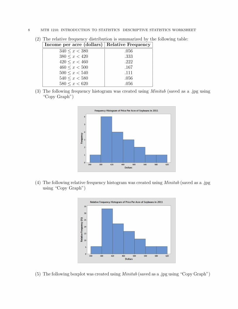
(3) The following frequency histogram was created using Minitab (saved as a .jpg using“Copy Graph”)

(4) The following relative frequency histogram was created using Minitab (saved as a .jpgusing “Copy Graph”)

(5) The following boxplot was created using Minitab (saved as a .jpg using “Copy Graph”)


(6) The following stem and leaf plot uses split hundreds digits for the stems:3 53 8894 0113334 57995 1145 9

(7) The mean is x̄ = 451.70.(8) The median is 437.50 .(9) The standard deviation is s = 62.80.

(10) The distribution reverse J-shaped and right-skewed.

Appendix B. Solutions to Practice Problems

Solution to Practice Problem 3.1:3.1(1): The frequency distribution is summarized by the following table:Class Frequency

ABC 4CBS 2NBC 6FOX 2

3.1(2): The relative frequency distribution is summarized by the following table:Class Frequency

ABC .286CBS .143NBC .429FOX .143

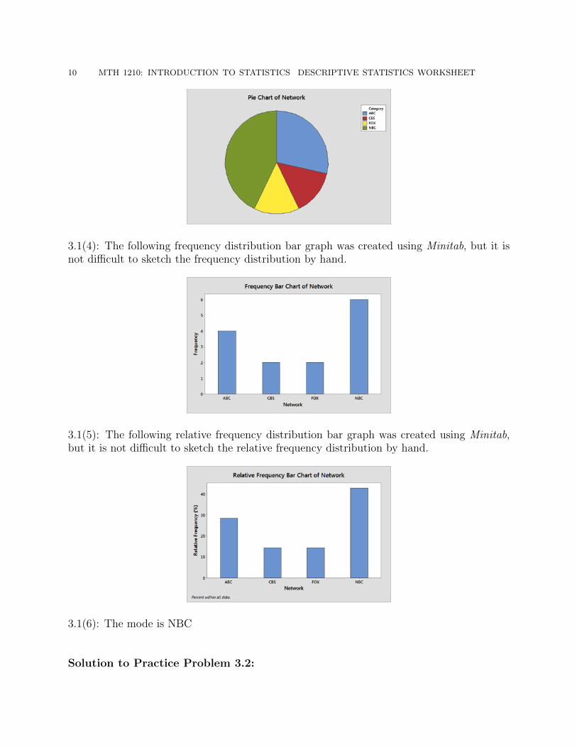
3.1(3): The following pie chart was created using Minitab, but it is not difficult to sketchthe pie chart by hand.


3.1(4): The following frequency distribution bar graph was created using Minitab, but it isnot difficult to sketch the frequency distribution by hand.

3.1(5): The following relative frequency distribution bar graph was created using Minitab,but it is not difficult to sketch the relative frequency distribution by hand.

3.1(6): The mode is NBC

Solution to Practice Problem 3.2:


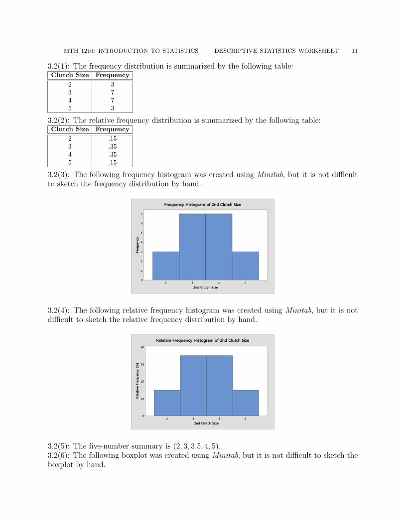
3.2(1): The frequency distribution is summarized by the following table:Clutch Size Frequency

2 33 74 75 3

3.2(2): The relative frequency distribution is summarized by the following table:Clutch Size Frequency

2 .153 .354 .355 .15

3.2(3): The following frequency histogram was created using Minitab, but it is not difficultto sketch the frequency distribution by hand.

3.2(4): The following relative frequency histogram was created using Minitab, but it is notdifficult to sketch the relative frequency distribution by hand.

3.2(5): The five-number summary is (2, 3, 3.5, 4, 5).3.2(6): The following boxplot was created using Minitab, but it is not difficult to sketch theboxplot by hand.


3.2(7): The mean is 3.53.2(8): The standard deviation is 0.946

3.2(9): The following double boxplot was created using Minitab, but it is not difficult tosketch the boxplot by hand.

Solution to Practice Problem 3.3:3.3(1): The frequency distribution is summarized by the following table:Income per acre (dollars) Frequency

180 ≤ x < 220 1220 ≤ x < 260 1260 ≤ x < 300 7300 ≤ x < 340 4340 ≤ x < 380 1380 ≤ x < 420 1420 ≤ x < 460 1


3.3(2): The relative frequency distribution is summarized by the following table:Income per acre (dollars) Relative Frequency

180 ≤ x < 220 .0625220 ≤ x < 260 .0625260 ≤ x < 300 .4375300 ≤ x < 340 .25340 ≤ x < 380 .0625380 ≤ x < 420 .0625420 ≤ x < 460 .0625

3.3(3): The following frequency histogram was created using Minitab, but it is not difficultto sketch the frequency distribution by hand.

3.3(4): The following relative frequency histogram was created using Minitab, but it is notdifficult to sketch the relative frequency distribution by hand.

3.3(5): The five-number summary is (218, 271.5, 289, 332, 445).3.3(6): The following boxplot was created using Minitab, but it is not difficult to sketch theboxplot by hand.


3.3(7): The mean is 308.13.3(8): The standard deviation is 573.3(9): The following boxplot was created using Minitab, but it is not difficult to sketch theboxplot by hand.

types of datasites.msudenver.edu/bdyhr/wp-content/uploads/sites/... · example, eye color of each...

Documents