Tying and Bundling in a Nearly Contestable Market

Michael A. Salinger*

Boston University School of Management

May 2011

Abstract: This paper presents a model of bundling and tying when the threat of entry provides the primary competitive constraint but entrants have a disadvantage with respect to the incumbent, i.e., in a “nearly contestable” market. The entrant’s disadvantage can be with respect to marginal costs, the fixed cost of a good, or the fixed cost of an offering (which can be interpreted as a product differentiation advantage). The incumbent’s profits depend on both the nature of its cost advantage and the set of offerings. With an advantage in the fixed cost of an offering, the incumbent prefers mixed bundling if it is sustainable. With a marginal cost advantage, the incumbent prefers pure bundling, in which all customers buy both components. While the latter result might appear to formalize a commonly-alleged rationale for tying, the practice can be a Pareto improvement over mixed bundling and can cause total consumer surplus to increase relative to only selling the products separately. Mixed bundling can lower consumer surplus and be a form of product proliferation.

Contact Information: Professor Michael A. Salinger Boston University School of Management 595 Commonwealth Ave. Boston, MA 02215 salinger@bu.edu 617-353-4408

I. Introduction

Tying is the practice of selling one good (the “tying good”) only in conjunction

with another good (the “tied good”). It is related but not identical to bundling, i.e., the

practice of selling two goods in combination with each other. Some firms sell bundles of

goods but also sell the individual goods separately, a practice known as mixed bundling.

When a firm ties, it does not sell the tying good separately.

Starting with Whinston (1990),1 much of the modern economics literature on

tying has concerned its use as an anticompetitive strategy. Carlton and Waldman (2002)

extend the basic logic of the Whinston model to settings that more nearly reflected the

broad facts underlying the government’s allegations in U.S. v. Microsoft.2 3 Choi and

Stefanadis (2001) formalize the idea that tying two monopolized complementary goods

can deter entry by preventing entry with only one. Nalebuff (2004) presents a model in

which bundling two economically independent4 products reduces the profits that a single-

1 In one of the Whinston models, a firm has a monopoly over two products, one of which is subject to entry and one of which is not. By tying the threatened product to the protected product, the monopolist commits to charging a low price for the bundle if entry occurs. The lower post-entry price of the incumbent reduces the profitability of entry and, given fixed costs for the entrant, can make the difference between entry being profitable and unprofitable. The second model in Whinston (1990) concerns a monopolist over two complementary products, “A” and “B.”. One of the products (A) is susceptible to entry by a superior alternative. The other product (B) is threatened by an inferior entrant. Absent the inferior potential entrant against B, the monopolist would actually benefit from entry by a superior competitor for A. But the potential entrant against B, while inferior, nonetheless limits the incumbent’s ability to raise the price of B. 2 Carlton and Waldman analyze a two-period model in which a monopolist over two complementary products faces potential entry for one of them in period 1 and the second product in period 2. By tying its two products in period 1, the incumbent can make initial entry in the one good unprofitable in period 1. The exclusion of the one good can then make entry into the second good unprofitable in period 2. As in Whinston, the entry deterrence comes from reducing the profitability of entry below the threshold needed to cover a fixed entry cost. Carlton and Waldman show that a similar effect arises when there are network externalities associated with the complementary good. 3 United States v. Microsoft, 253 F.3d 34 (D.C. Cir. 2001). 4 Here, “economic independence” means that the goods are neither substitutes nor complements. That is, the demand for one is not a function of the price of the other. Economic independence does not imply statistical independence. There is a substantial body of literature that explores the effect of the statistical non-independence of the demand for the two products on offerings and prices.

product entrant can earn and thereby can prevent entry altogether.5 Carlton, Gans, and

Waldman (2010) present a model in which the monopolist over one good might tie an

inferior complementary good to its monopolized offering to reduce the rents available to

the seller of a superior version of the complementary good.

From the economics literature on tying, one might get the impression that

exclusion is the primary reason that firms tie one product to another. To be sure, many of

the articles point out that tying can provide convenience or lower costs, but these

explanations typically receive only passing mention and, more importantly, fail to

distinguish between bundling and tying. Although not, strictly speaking, an efficiency,

another strand in the literature, dating back to Stigler (1963), is that tying can be a form

of price discrimination. Again, though, this explanation typically fails to distinguish

between bundling and tying. In fact, the economics literature does not contain an

accepted general explanation for why firms tie, i.e. why they refuse to sell the tying good

on a stand-alone basis even if some purchasers of the bundle do not want the tied good.

By a “general explanation,” I do not mean a general theory that captures all possibilities.

Rather, I mean an accepted (by economists), compelling explanation for the typical case.6

At least as it is typically articulate, the efficiency explanation is not compelling. A

commonly-cited example of tying because of efficiencies is selling shoes in pairs. But

the savings from placing two shoes in a box rather than in separate boxes are marginal

cost savings that explain why firms sell pairs of shoes to the vast majority of people who

5 See, also, Nalebuff (2005). 6 A significant class of tying cases concerns durables and consumables (such as printers and ink). There is probably a consensus among economists that the typical motive for tying a consumable to a durable is to charge based on usage. I would count this “metering” explanation as a general explanation for that form of tying. What is lacking is a general explanation for “packaged tying,” i.e., the sale of two goods in a package but not separately. A prominent example of packaged tying was Microsoft’s decision to sell Windows only with its web browser, Internet Explorer.

2

want both shoes.7 Those marginal cost savings cannot explain why most shoe

manufacturers do not sell single shoes to the rare individual who wants just one. The

same point applies to convenience. If people who want both goods in a bundle find it

more convenient to buy them in a single package rather than separately, then bundling

adds value for those who want both goods. But for people who have no use for one of the

goods in the bundle, it simply creates the need to dispose of the unwanted item.

Similarly, the price discrimination explanation is far more compelling as a theory of

mixed bundling than it is of tying.8

The lack of a generally accepted explanation for tying is particularly problematic

because tying can be an antitrust violation. At one point, Microsoft - at the time the

world’s largest company measured by market capitalization - was under a United States

district court divestiture order for tying its web browser to its Windows operating system.

To be sure, serious commentators understood the need to articulate what distinguished

the tying of Internet Explorer to Windows not only from the ties routinely observed under

competition but also the other examples of tying by Microsoft.9 One must be cautious,

however, about identifying the salient features of the rare exception without

understanding the typical case.10 In Jefferson Parish v. Hyde, the prevailing United

States Supreme Court precedent on tying, the Court ruled, “[T]he essential characteristic

of an invalid tying arrangement lies in the seller's exploitation of its control over the tying

7 As Mark Frankena has pointed out to me, there is some demand for individual shoes. See NLLIC ACA Fact Sheet: Mismatched and Single Shoes, at http://www.amputee-coalition.org/fact_sheets/oddshoe.html (last visited April 1, 2011). 8 As a further example of what I mean by a general explanation, the general explanation for why firms practice (or want to practice) minimum resale price maintenance is to prevent free riding from retailers who rely on other retailers that provide costly services that are of value to a manufacturer. 9 Carlton and Waldman (2002) is a notable example. 10 Some of the authors of papers on the potential anticompetitive effects of tying have been careful to point this out. See Whinston (1990) at 855-6, Whinston (2001) at p. 79, and Carlton and Waldman (2001), at pp. 215-16.

3

product to force the buyer into the purchase of a tied product that the buyer either did not

want at all, or might have preferred to purchase elsewhere on different terms.”11 But

people purchase bundles that include goods they do not want even in competitive

markets. To take a prominent current example, Southwest Airlines has heavily promoted

the fact that it ties the right to check two bags to its passenger service.12 Air travelers

without luggage to check would presumably decline to purchase the right to check a bag,

so Southwest passengers end up purchasing something they do not want.13 As a result,

the legal standard for the essence of an invalid tying arrangement fails to distinguish it

from the sorts of tying arrangements that we observe under sufficiently competitive

circumstances to presume that they are efficient or, at the very least, a form of

competition.

The analysis of why a firm does not offer a good separately even though there is

demand for it is an issue of product selection.14 In one strand of the literature on product

selection, there are diverse customer preferences for product characteristics and scale

economies that prevent companies from giving each customer the precise product

characteristics he or she wants. Those models are all based on a demand structure that

tries to capture general product differentiation. To adapt that broad framework to

bundling and tying, two steps are essential. First, one needs a demand structure that

captures multiple goods that can be sold separately or as part of a bundle; and, second,

11 Jefferson Parish Hospital Dist. No. 2 v. Hyde, 466 US 2, 12 (1984). 12 While the airline market is neither perfectly competitive nor, as is discussed below, perfectly contestable, Southwest Airlines is neither a monopolist nor a dominant firm; and its strategy with respect to bags is almost surely aimed at increasing current profits rather than sacrificing current profits to drive out rivals. 13 Another important feature of this example is that the change in the technology of transactions has almost surely been a key factor in making it feasible for Southwest’s competitors to charge for checked bags. The traditional practice of tying the right to check two bags to passenger service reduced transactions costs by simplifying the set of product offerings. 14 See Spence (1976), Dixit and Stiglitz (1977), and Salop (1979).

4

one needs to recognize that bundles are distinct product offerings from the individual

goods and that there are scale economies associated with the offering (as distinct from the

individual goods).

Evans and Salinger (2005, 2008) put forward a candidate general explanation for

tying with these features. In the model’s starkest form, the underlying assumptions are

that there are two goods and three types of consumers. One of the groups wants just

“good 1;” one of the groups wants just “good 2;” and the third group wants both. The

seller has constant marginal cost of producing both goods and the bundle, and the

marginal cost of the bundle might be (but is not necessarily) less than the sum of the

marginal costs of the individual goods. The assumption that distinguishes the Evans-

Salinger model from previous models of tying is that each offering entails a fixed cost,

where the bundle is a separate offering from the individual goods.15 They argue that a

fixed offering cost is essential to understanding tying (as distinct from bundling) – i.e.,

the refusal to sell the precise good that some customers want. Given the scale economies

implied by their technological assumptions, competition in the Evans-Salinger cannot

mean perfect competition. Instead, they assume that markets are perfectly contestable.

In the Evans-Salinger model, pure bundling, a form of tying, can occur under two

distinct circumstances. One is that most customers want both goods and bundling saves

marginal costs. Under such circumstances, only modest fixed costs of an offering make it

impossible for an entrant to profitably sell the individual goods at a price below what the

incumbent charges for the bundled product. Selling shoes in pairs is the prototype of this

case. In the other, pure bundling arises even if no one wants both goods and bundling

does not lower marginal cost. While perhaps counterintuitive at first, the condition 15 Carlton, Gans, and Waldman (2010) have since introduced this feature into their model.

5

generating the result turns out to be obvious. When the fixed cost of an offering is large

enough, a single bundled product can be the most efficient way to meet the needs of

customers with diverse tastes. Pure bundling for this reason is common. Few if any

people want all of a newspaper or magazine. Few students take advantage of all the

services to which they are entitled by virtue of paying university tuition.16

Two features of the Evans-Salinger model arguably make it problematic as a

general explanation for tying. First, the assumption of perfect contestability is quite

strong. It excludes by assumption any strategy to generate economic profit. Second,

while the Evans-Salinger model allows for offering-specific scale economies, it assumes

away product-specific scale economies. These scale economies are generally essential

features of models of anticompetitive tying as in Winston (1990) and Nalebuff (2004).

As a result, when both product-specific and offering-specific scale economies are present,

it is not clear how one would determine whether a model of anticompetitive tying or a

model of competitive tying provides the more plausible explanation.17

This paper generalizes the Evans-Salinger model to remedy these two

shortcomings. It augments the underlying assumptions about technology by introducing

a fixed cost of producing each good (regardless of whether it is sold separately or as part

16 A relatively recent example of unbundling that is of academic interest concerns college textbooks. Many college textbooks contain more chapters than a professor can cover in a single course. Including more material than is needed for any one class allows a single textbook to meet the needs of many professors with diverse tastes for what to cover. Some college textbook publishers customize versions to include just the subset of chapters a professor wants and discount the customized versions substantially with respect to the full text. No doubt, technical change that has reduced the fixed cost associated with a version is a substantial portion of the explanation. However, from discussions with textbook representatives, my understanding is that another part of the explanation is that customized versions have much less resale value than do the full versions. Given the resale market, textbook publishers do not want a single product that meets diverse customer needs. 17 As Winston (2001) pointed out, a rational choice between explanations for any particular instance of tying requires prior beliefs based on the relative frequency of pro- and anti-competitive tying. As objective measures of the relative frequency are not now available and are unlikely to become available in the foreseeable future, such priors must be subjective.

6

of a bundle). In addition, it relaxes the perfect contestability assumption by assuming

that markets are “nearly contestable.” While Section IV contains a more precise

definition, the incumbent in a nearly contestable market has some advantage over

potential entrants. As a result, the threat of entry does not compel average cost pricing

and therefore does not preclude economic profits. At the same time, however, the threat

of entry remains the primary competitive constraint on the incumbent’s decisions about

prices and product offerings.

The results in this paper stem from a simple insight about nearly contestable

markets: An incumbent’s profits are limited by its cost advantage, which in turn depends

both on the set of offerings and on whether the cost advantage concerns marginal costs,

fixed offering costs, or fixed product costs. This insight yields a rich set of results. With

an advantage in fixed offering costs, the incumbent’s cost advantage is greatest with

mixed bundling, which does not entail tying, because mixed bundling entails the greatest

number of offerings. With an advantage in marginal costs, the incumbent’s cost

advantage is greatest with pure bundling, which does constitute tying.

The effect on consumers of tying or untying can be counterintuitive. In cases

when an incumbent chooses mixed bundling to deter entry by firms selling just the goods

separately, consumer surplus can drop. Offering the bundle at a discount to the sum of

the prices entrants would charge for the goods sold separately denies part of the market to

the entrants and allows the incumbent to increase the price it charges for the goods sold

separately. On the other hand, when the firm chooses pure bundling to deter entrants

who would do mixed bundling, consumers benefit. On the surface, the practice might

appear to force all consumers to buy both products because that is what maximizes the

7

incumbent’s cost advantage. However, the strategy only succeeds if the incumbent’s

price for the bundle matches the price the entrants get for the individual products.

Consumers who want both goods get them for the price an entrant would charge for just

one.

An incumbent advantage with respect to fixed product costs is constant across

sets of product offerings, so it does not create a preference for tying or untying.

However, fixed product costs create a disadvantage for an entrant seeking to sell an

offering to just one set of consumers (eg., selling product 1 to customers who want just

product 1) even if the incumbent bears the same cost. With product fixed costs, there is a

greater tendency for multiple sets of product offerings to be sustainable and therefore

greater scope for the incumbent to choose the set it prefers.18

The remainder of the paper is organized as follows. The following section

provides a brief summary of the controversy over the usefulness of the contestability

assumption and argues that economists have been wrong to dismiss it. Section III covers

bundling and tying in a perfectly contestable market. It reviews the Evans-Salinger

model and then extends it to allow for fixed product costs. Section IV defines “nearly

contestable markets” and analyzes the incumbent’s bundling and tying decisions in them.

Section V contains a summary and conclusions.

18 That is, fixed product costs lower the marginal cost advantage an incumbent needs to choose pure bundling when entrants would choose mixed bundling. They also lower the fixed cost advantage an incumbent would need to choose mixed bundling to prevent entry by firms that would sell the goods separately.

8

II. The Rise and Premature Fall of the Contestability Assumption

In the late 1970’s and through the 1980’s, the theory of contestable markets was a

hot and hotly debated topic in industrial economics.19 Originally developed in the

context of the Department of Justice’s monopolization case against AT&T,20 it played a

prominent role in the debates about airline deregulation.21 A central issue in those

debates was whether market outcomes would be sufficiently competitive, particularly on

routes where demand would support at most a small number of carriers. Because the

opportunity to reallocate airplanes among routes made entry onto and exit from

individual routes appear easy, some argued that airline markets might be perfectly

contestable. That is, the threat of entry would force competitive pricing even on highly

concentrated (or even monopoly) routes.

Some of the critiques of the contestability assumption were theoretical. The

contestability literature made a great deal of the distinction between fixed and sunk costs.

Weitzman (1983) criticized the distinction as being fundamentally illogical. Stiglitz

(1987) argued that contestability models are not robust to even small sunk costs. Shwartz

(1986) focused on the relative speed of entry, exit, and incumbent price responses.

19 For background on the theory of contestable markets, see Buamol, Panzar, and Willig (1982) and Baumol (1982). 20 Telecommunications, particularly in the 1970’s and 1980’s, might seem an odd application of contestability theory, as sunk costs were substantial. However, a fundamental issue in the antitrust case as well as some key regulatory proceedings that led up to it was whether financial success by an entrant would demonstrate the efficiency of entry. A major contribution of the literature was to extend the concept of natural monopoly to multi-product settings and to address the question of whether it would be possible to have a set of prices that would cover the costs of a multi-product natural monopolist and also be immune from inefficient entry. 21 See Bailey and Panzar (1981) for the suggestion that airline markets might be contestable.

9

Other critiques were empirical. Because the mere threat of entry forces in effect

perfectly competitive behavior, actual entry and the number of existing competitors

should not affect pricing. As a result, any evidence linking actual market structure to

prices contradicts the contestability hypothesis. The evidence that may have contributed

most to the rejection of the contestability assumption concerns airlines, an industry for

which it was considered well-suited. Several studies have obtained results that airfares

are statistically related to the number of actual competitors as well as the number of

likely potential competitors.22 Morrison and Winston (1987) showed that both the

number of existing competitors and the number of likely entrants were statistically

significant predictors of air fares. They concluded that airline markets are “nearly

contestable,” a hypothesis that they considered to be dramatically different from

“perfectly contestable.” Writing in The Journal of Economic Perspectives in 1989,

Gilbert wrote: “There is only weak evidence consistent with … [perfect contestability],

and the amount of inconsistent evidence is substantial….” Echoing Stiglitz, Gilbert went

on to argue, “[A] theory that applies only when entry and exit costs are strictly zero is of

little practical use.” But he then stated the key issue perfectly: “The central question is

whether contestability theory makes useful predictions about markets that are close to

being perfectly contestable.”[p. 124]

Statistical rejection of a model simply means that it is highly unlikely to be

literally true. But models are supposed to be approximations, not literal truth; so

rejecting the hypothesis of perfect contestability does not resolve the question of what

role entry should play in modeling markets. An important case to consider is the prices

Microsoft has charged historically for its Windows operating system. This was a central 22 See Morrison and Winston (1987), Borenstein (1989), and Borenstein (1992).

10

point in Microsoft’s defense of the monopolization suit against it.23 During the time at

issue in the suit, the license fee Microsoft charged computer manufacturers for Windows

was reputed to be $50-$65 while the typical price for a computer was $2,000. The

demand for the operating system is a derived demand based on the demand for

computers. Since the price of Windows represented less than 4% of the price of the

typical computer, any plausible estimate of the elasticity of demand for computers would

imply that Microsoft was operating in the inelastic portion of the demand curve. Taking

account of the sale of complementary software would lower an estimate of the profit-

maximizing price for Windows, but the effect was not nearly large enough to rationalize

the price Microsoft was charging as an unconstrained monopoly price. There is little

controversy that Microsoft had been highly profitable, so perfect contestability would not

be a plausible assumption about Microsoft’s pricing and other behavior. However,

unconstrained monopoly as an assumption arguably fails even worse than perfect

contestability. To the extent that Microsoft’s pricing of Windows is evidence for the

constraining effect of potential entry, the question then becomes how to incorporate that

assumption into a tractable model.

The model presented below is tractable, allows the threat of entry to be the

primary competitive constraint on the incumbent firm, but does not force it to forego all

economic profits without actual competition.24

23 See Reddy, Evans, and Nichols (2002). 24 One interpretation of the results of a model of “near contestability” is that it captures what a hypothetical monopolist would do. An important avenue for future research is to incorporate oligopolistic interdependence among multiple incumbents. This might prove to be a tractable approach to simultaneously modeling the threat of entry and existing competition

11

III. Bundling and Tying under Perfect Contestability

The underlying assumptions of the model are similar to those in Evans and

Salinger (2005, 2008). A monopolist sells two goods, 1 and 2, that it can sell separately

and/or in bundled form. There are three groups of customers, denoted groups 1, 2, and B.

Members of group 1 want just good 1. Members of group 2 want just good 2. Members

of group B want both. Members of all three might obtain the good(s) they want in one of

two ways. Members of groups 1 and 2 might buy just the good they want or they might

buy the bundle and discard the good they do not want. Members of group B might buy

the bundle or the two goods separately.

To make the exposition clearer, I make four simplifications. First, I consider only

symmetric parameters (in which the demand for and the cost of the two goods sold

separately) are equal. Second, I assume that each group’s demand for the good it wants is

perfectly inelastic. Let XS be the size of groups whose members get value from a single

product (i.e., Groups 1 and 2) and XB be the size of the group that wants both products.

Third, consumers in each group are indifferent between purchasing the good(s) they want

separately or in bundles. These assumptions make it possible to illustrate the points with

simple numerical examples.25 Fourth, with one exception in Section IV, I consider only

symmetric strategies.26

A. Costs

The incumbent incurs a constant marginal cost cS for the production of separate

good and cB for the production of the bundled product. Assume cS ≤ cB ≤ 2cS. The 25 Evans and Salinger (2008) relax all these assumptions for perfect contestability. 26 That is, by assumption, the incumbent does not offer the bundle and just one of the separate products.

12

incremental (and wasted) marginal cost of providing the bundle to consumers who want

just one product is cB – cS. The marginal cost savings from providing the bundle rather

than the separate products to consumers who want both is 2cS – cB. A key assumption is

that the incumbent incurs a fixed cost, F, for each offering, where Goods 1 and 2 and the

bundle are separate offerings. This fixed cost is associated with the offering, not the

production of Goods 1 and 2. I also allow for a fixed product (or good) cost, G.27

B. Sustainability conditions under perfect contestability

A possible market outcome is a set of offerings and associated prices that are

“sustainable,” which means that the offerings and prices are immune from entry either by

a company offering the same set of offerings or an alternative set that would allow it to

undercut the incumbent and break even. Given the symmetry assumption, there are three

possible sets of offerings. Under “mixed bundling,” all three offerings are available.

Only the bundle is available under “pure bundling.” The two goods are available

separately but not bundled under “components selling.”

To be sustainable against entry by a firm with the same set of offerings as the

incumbent, prices must result in zero economic profits. Under both pure bundling and

components selling, there is a unique “break-even” price (equal to average cost) for each

offering. Let B be the price of the bundle under pure bundling and P be the price of each

good sold separately under components selling. For mixed bundling, there is a range of

break-even prices depending on the allocation of the fixed product costs between the

bundle and the individual products. Because of the break-even constraint, there is a

trade-off between the prices of the separate products and the price of the bundle within 27 To keep the notation simple, I assume entrants’ fixed cost disadvantages are equal across offerings and products.

13

this range. With k (0 ≤ k ≤ 1) being the fraction of fixed product costs allocated to the

separate products under mixed bundling, let MS (k) and MB (k) represent the range of

break-even prices for the separate products and the bundle, respectively, under mixed

bundling.28

1. No Fixed Product Costs

The analysis of what product offerings are sustainable is simpler when there are

no fixed product costs. In that case, which product configurations are sustainable

depends on which of three basic conditions hold.29 The first is the “separate products

stand-alone condition”:30

Error! Bookmark not defined.(1) ( ) .1 BM S <

The left-hand side of (1) is the price an entrant would have to charge if it tries to sell just

a separate product to the group that wants just that product. The right-hand side is the

price of the bundle under pure bundling. If equation (1) holds, any sustainable set of

product offerings must include the separate products,31 which rules out pure bundling.

Similarly, the “bundle stand-alone condition” is:

(2) ( ) .20 PM B <

28 As is explained below, the entire range is not necessarily sustainable under mixed bundling. An entrant seeking to sell one offering to one group would, however, have to allocate the entire fixed product cost(s) just to that offering. 29 Without the symmetry assumption, there are six conditions. See Evans and Salinger (2008). 30 With no fixed product costs, the prices under mixed bundling do not depend on k. However, equations (1) and (2) are stated with values of k that generalize to when there are fixed product costs. 31 With asymmetric demand and costs, there is both a strong and weak version of the stand-alone conditions for separate products.

14

The left-hand side of (2) is the price an entrant would have to charge to sell the bundle just

to the group that wants both products. If it holds, pure components selling is not sustainable.

The third condition is the “pure bundling sufficiency condition:”

(3) .PB<

If it holds, a firm selling the bundle to all can undercut a firm selling the goods separately

even for the customers who want just one of the goods.

With these conditions, we can state Theorem 1:

Theorem 1: Assume there are no fixed product costs. Equation (3) implies that pure bundling is the only sustainable set of product offerings. If equation (3) does not hold, then: a) if equations (1) and (2) hold, mixed bundling is the only sustainable set of product offerings; b) if equation (1) holds but equation (2) does not, components selling is the only sustainable set of product offerings; c) if equation (2) holds but equation (1) does not, pure bundling is the only sustainable set of product offerings; and (d) if neither equation (1) nor (2) holds, both pure bundling and components selling are sustainable, but mixed bundling is not.

The proof is evident given the definition of sustainability and the equations.

Tables 1-5 contain numerical examples of the five possible qualitative outcomes. In

Table 1, mixed bundling is the sustainable outcome. The marginal cost of a separate

product is 25. The marginal cost of the bundle is 35, so bundling entails marginal cost

savings of 2 x 25 – 35 = 15. Fixed offering costs are 1,500. 100 customers want each

separate product; 50 customers want both. The break-even prices are 35 for the separate

products under components selling, 40 for the separate products and 65 for the bundle under

mixed bundling, and 41 for the bundle under pure bundling. Equation (1) holds because the

price of separate products under mixed bundling (40) is less than the bundle price under

pure bundling. Equation (2) also holds because the price of the bundle under mixed

15

bundling (65) is less than the sum of the prices of the separate goods under components

selling (2 x 35 = 70).

In Table 2, the parameters are the same as in Table 1 except that the marginal cost of

producing the bundle is 45, not 35. With a smaller marginal cost savings from bundling,

components selling is the unique sustainable outcome. The bundle price under mixed

bundling, 75, is greater than the sum of the prices of the separate products under

components selling. Thus, equation (2) does not hold, but equation (1) does.

In Table 3, the parameters are the same as in Table 2 except for the size of the

different customer groups. 200 consumers want both goods is 200 while demand for each

separate good is only 50. Equation (1) does not hold, but equation (2) does, so pure

bundling is the only sustainable outcome.32

Table 4 exemplifies the other class of pure bundling cases. In Table 3, most

customers want both products. Some want the separate products, but not enough to sustain

separate offerings in light of the fixed offering cost (as well as the marginal cost savings

from bundling). In Table 4, no customer wants both products and bundling does not save

marginal costs. Yet, pure bundling is the only sustainable outcome. The price of the bundle

under pure bundling is 80, which is less than the price of 85 for the individual products

under components selling.33 Because of the high fixed offering cost of 6,000, equation (3)

holds. Having a single bundled product satisfies the needs of both groups of customers with

a single offering.

32 Mixed bundling is not sustainable because the price of 50 with pure bundling is lower than the price of the separate products under mixed bundling (which is why equation (1) does not hold). Those who want just one of the products would prefer components selling with P = 31 to pure bundling. That outcome is not sustainable, however, because it is not immune from entry by a company selling the bundle just to those who want both products. 33 Since no one wants both products, mixed bundling would not be feasible since there would be no demand for the bundle.

16

Table 5 illustrates the final qualitative possibility. None of equations (1) – (3) hold,

so components selling and pure bundling are both sustainable. Multiple outcomes can be

sustainable in a contestable market because a successful entrant has to beat the incumbent

with respect to all its (i.e., the entrant’s) intended customers. Thus, in Table 5, customers

who want both products prefer the bundle at 52, the price under pure bundling, to the two

separate products at 45 each. However, if the incumbent charges 45 for the components, an

entrant cannot offer the bundle at 52 because the customers who want just one of the

products will not purchase from the entrant. Without selling to those customers, the entrant

cannot achieve average costs of 52.

Given the assumption of perfectly inelastic demand, welfare maximization is

equivalent to cost minimization. Under the assumptions above, pure bundling and

components selling are efficient when they are the unique sustainable outcome.34 When

pure bundling and components selling are both sustainable, which one entails lower costs

depends on the precise parameters. In these cases, the efficient outcome is sustainable, but

so is a less efficient outcome. There is no compelling reason under perfect contestability

why one outcome should prevail over the other. Under near contestabity, however, the firm

will generally have a preference among multiple sustainable outcomes.

Again given perfect contestability, mixed bundling occurs when it is efficient, but

the converse is not true. Mixed bundling can be sustainable even though it is inefficient

because of a type of negative externality from the addition of an offering. Consider, for

example, adding the bundle when the two goods are available separately. Doing so is

efficient if the average cost of the bundle (including the average fixed offering cost) is less

34 See Evans and Salinger (2008) for an analysis of the relationship between sustainable and efficient outcomes in their modeling of bundling and tying.

17

than the sum of the marginal costs. The bundle is sustainable, however, as long as the

average cost of the bundle is less than the sum of the average costs, which include an

allocation of the fixed offering costs, of the two components. Ths savings to group B from

not having to share in the fixed offering costs of the individual goods is not a social benefit.

Instead, the consumers who want just one of the goods have to pay for the portion of the

fixed offering costs that the members of group B would have paid under components

selling.

2. Fixed Product Costs

With fixed offering costs but no fixed product costs, there are no joint costs between

offerings. Thus, an entrant with a single offering has no inherent total cost disadvantage

compared with an incumbent that can sell to all groups of customers.35 With mixed

bundling, however, fixed product costs are joint between the bundle and the separate

product. An incumbent practicing mixed bundling would therefore have an advantage over

an entrant with a single offering aimed at a single customer group. Formally, a firm seeking

to sell just a single product to the group that wants it must charge MS(1) (because k = 1

means that the entire fixed product cost is allocated to the separate product); and a firm

seeking to sell the bundle just to Group B must charge MB(0). In contrast, the incumbent

can capture part of the fixed product costs with sales to the other group that wants the

product(s).

With fixed product costs, equation (1) still implies that pure bundling is not

sustainable. However, entry by a firm selling a separate product at average cost is no

35 The incumbent’s first mover advantage does give it an average cost advantage.

18

longer the only competitive threat to a pure bundler. It also faces potential competitive

from a mixed bundler. In analyzing this threat, the entire feasible range of prices is

relevant. However, even though we can define MS(k) and MB(k) over 0 ≤ k ≤ 1, not all

values are feasible because MB(k) must fall within the range [MS(k), 2 MS(k)]. If MB(k)

were below that range, customers who want just one product would buy the bundle. If it

were above that range, customers who want both products would buy them separately.

Define kL* and kH* so that they satisfy:

(4) MS(kL*) = MB(kL*)

(5) MB(kH*) = 2 MS(kH*).

Then, kL = max(0, kL*) and kH = min(1, kH*) define the feasible range for k.

For an entrant that practices mixed bundling to succeed against an incumbent

practicing pure bundling, it must beat the incumbent with respect to all groups. Since a

feasible mixed bundling strategy requires MB(k) > MS(k), an entrant that provides group B

with a better price will necessarily do so for groups 1 and 2 as well. The lowest feasible

price for the bundle under mixed bundling is MB(kH), so equation (6) is a condition under

which pure bundling is not sustainable:

(6) MB(kH) < B.

The other possibility to consider for how pure bundling might be susceptible to

entry is for an entrant to sell just the two components. However, unless cB > 2 cS, in

which case bundling would increase marginal costs, 2 P > B, so a firm selling the two

separate products cannot offer a better price to group B than it gets under pure bundling.

Thus, we can state the following theorem:

Theorem 2: Pure bundling is not sustainable if either equation (1) or equation (6) holds. If neither is true, pure bundling is sustainable.

19

Now consider components selling. Without fixed product costs, components

selling is not sustainable if either equation (2) or (3) holds. Either remains sufficient for

components selling not to be sustainable. However, components selling is also

susceptible to entry if:

(7) MS(kL) < P

This implies:

Theorem 3: Components selling is not sustainable if equations (2), (3), or (7) hold. If none holds, components selling is sustainable.

Finally, consider mixed bundling. First note under mixed bundling, an entrant

cannot succeed simply by choosing a different value for k. A successful entrant has to

attract all groups and a different value for k would necessarily offer a worse deal to at

least one.

If equations (1) and (2) both hold, mixed bundling is sustainable (and, indeed, the

only sustainable outcome). Without fixed product costs, mixed bundling would not be

sustainable when (1) or (2) do not hold. However, with fixed product costs, mixed

bundling can occur in a wider range of circumstances. Define kB and kC as:

(8) MS(kB) = B

(9) MB(kC) = 2P .

Equation (8) defines an allocation of the product fixed costs between the components and

the bundle so that the price of the components matches what a pure bundler can offer (to

those who want just one of the products). Any lower price for the separate products

(based on k < kB) insulates a mixed bundling incumbent from entry by a pure bundler.

Equation (9) defines an allocation so that the price of the bundle matches the sum of the

20

prices under components selling. Any lower price of the bundle (based on a k > kC)

insulates the incumbent from entry by a firm that practices components selling. Thus, as

long as kB > kC, kB > kL, and kC < kH, then mixed bundling is sustainable. This implies:

Theorem 4: Mixed bundling is sustainable if both equations (1) and (2) hold. It is also sustainable if kB > kC, kB > kL, and kC < kH, where equations (4), (5), (7), and (8) define kL, k H, kB, and kC.

To understand the effect of fixed product costs, modifications of the examples in

Tables 1, 3 and 5 are useful. In Table 6, the parameters are similar to Table 1 except that

there are fixed product costs of 600 and the fixed offering cost of 1,500 is reduced to 900.

The combination leaves the average cost under components selling unchanged, so P = 35,

just as in Table 1. When k = 0, i.e., when the entire fixed product costs are allocated to

the bundle, the bundle price of 77 is more than double 34, the price of the separate

products.36 Thus, k = 0 is not feasible. The minimum feasible value for k is 0.25, which

yields a price for the separate products of 35.5 and a bundle price of 71. The value for kC

is 0.29, which gives a bundle price of 70 and a price for a separate product of 35.8. Any

higher value of k gives a lower bundle price and therefore a price below the sum of the

prices of the separate products under components selling. The prices for k = 1 are

feasible, so kH = 1. The value for k that equalizes the prices of a separate product and the

bundle is 1.60, which is outside the feasible range.

Recall that in Table 1, mixed bundling is the unique sustainable outcome. This is

no longer the case. Equation (1) holds. A firm selling a single product just to the group

that wants just that product can charge 40, which is less than 43.4, the price of the bundle

36 Recall that with k = 0, the product fixed costs are allocated entirely to the bundle. Thus, buying the products separately is the better option for those who want both goods. The strategy would fail because it is premised on recouping the fixed product costs from Group B by getting them to pay 77 for the bundle, which they would not do.

21

under pure bundling. Thus, pure bundling is not sustainable. However, equation (2) does

not hold. A firm seeking to enter with just the bundle to sell to Group B would have to

charge 77, which would not capture group B from a firm selling the two separate

products for 35. Thus, components selling is sustainable. Mixed bundling is also

sustainable with k > kC = 0.29, which ensures that the price of the bundle is less than the

sum of the prices of the separate goods under components selling.37

Table 7 is based on Table 3 but with product fixed costs of 300 and offering fixed

costs of only 1,200. As in Table 3, components selling is not sustainable because

equation (2) holds. Equation (1) does not. In addition, at the highest feasible value of k,

the price of the bundle (as well as a separate product) is 52.3, which exceeds the price of

the bundle under pure bundling of 51. Thus, pure bundling is immune from entry by a

firm practicing mixed bundling. In contrast to Table 3, however, mixed bundling (with k

< 0.33) is sustainable. With sufficiently low portions of the fixed product costs allocated

to the separate products, a firm practicing mixed bundling can charge low enough price

for the separate products that a firm practicing pure bundling cannot attract Groups 1 and

2.

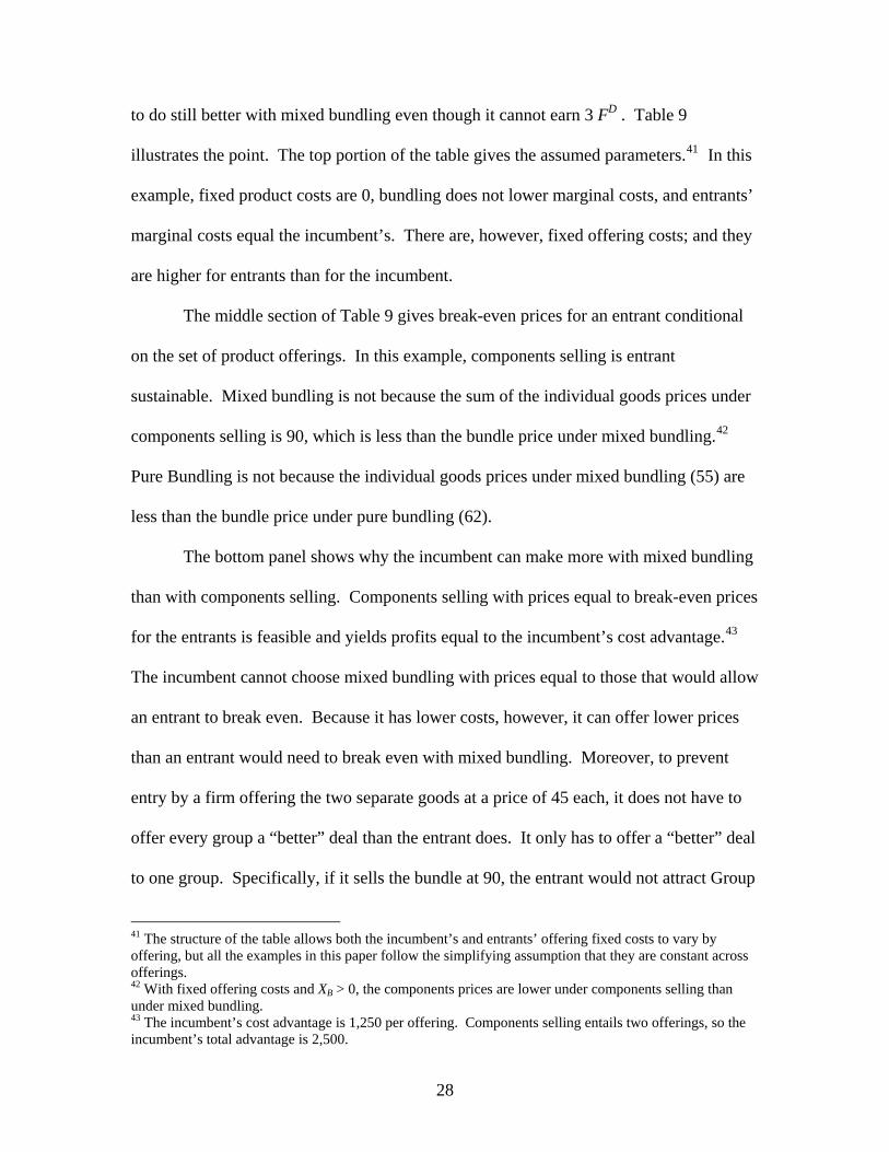
Table 8 has parameters similar to Table 5 except that there are fixed product costs

of 700 and fixed offering costs are 2,300 rather than 3,000. Recall that in Table 5, both

pure bundling and components selling are sustainable, but mixed bundling is not. In

Table 9, components selling and pure bundling remain sustainable, but mixed bundling is

sustainable as well with 0.86 < k < 0.97.

37 Modifying Table 2 in a similar way – i.e., by adding fixed product costs of 600 and reducing fixed offering costs by the same amount – also results in both components selling and mixed bundling being sustainable.

22

While Tables 6-8 do not exhaust the possible outcomes with fixed product costs,

they demonstrate the sense in which fixed product costs make it more “likely” that there

are multiple sustainable outcomes. Without fixed product costs, mixed bundling is either

the only sustainable outcome or it is not sustainable. With fixed product costs, mixed

bundling can be sustainable for parameters where other outcomes are also sustainable,

and all three qualitative outcomes can be sustainable for some parameter values.

IV. Near contestability

In a perfectly contestable market, the threat of entry is the operative constraint on

the incumbent’s prices and potential entrants are just as efficient as the incumbent. As a

result, the incumbent cannot charge a price above its own average cost or earn economic

profits. The assumption of “near contestability” preserves the first of these assumptions

but not the second. Potential entrants constrain prices, but they have some cost

disadvantage relative to the incumbent. As a result, the incumbent is not forced to lower

its prices to its own average cost.

The cost disadvantage can take one of three forms: marginal costs, fixed offering

costs, and fixed product costs. Let csD be an entrant’s marginal cost disadvantage for a

separate product, cBD be the entrant’s marginal cost disadvantage in producing the bundle,

FD be the entrant’s fixed offering cost disadvantage, and GD be the entrant’s cost

disadvantage with respect to fixed product costs.38 While the fixed offering cost is

essential for understanding tying, the possibility that an entrant’s disadvantage might

stem from this type of cost might seem contrived at first. However, what matters about

38 The difference between these fixed offering costs and fixed product costs is that the latter is a common cost for product sold separately and as part of a bundle.

23

the fixed cost is its size relative to the number of purchases. Suppose that some

customers would be unwilling to purchase the entrant’s product. That is, suppose there is

a product differentiation barrier to entry. If so, the entrant would need a higher price to

break even than would the incumbent to cover its higher fixed cost per customer.

Under “near contestability” with a single product, the incumbent charges the

entrant’s average cost and earns an economic profit per unit equal to the difference

between the entrant’s average cost and its own.39 To extend the analysis to the

multiproduct, define “entrant sustainable” prices as:

Definition: Suppose an incumbent faces potential entrants with costs that are 1) equal to each other and 2) weakly greater than the incumbent’s. Prices (and the associated set of product offerings) are “entrant sustainable” if they would be sustainable if 1) all firms (including the incumbent) had costs equal to those of the potential entrants and 2) the market was perfectly contestable.

Given this definition, all the results from the previous section about sustainable

outcomes in a perfectly contestable market apply to Entrant Sustainability in a nearly

contestable market with the qualification that the conditions depend on entrants’ costs,

not the incumbent’s.

We can establish the following lemma:

Lemma 1: If the market is nearly contestable, any Entrant Sustainable set of offerings and prices is feasible for the incumbent. If it chooses an Entrant Sustainable set of offerings and prices, the incumbent’s economic profits are equal to its cost advantage over the potential entrants given the set of offerings.

The first part of the lemma is an obvious implication of the definition of entrant

sustainable prices. The second part follows because the revenues from an entrant

sustainable set of offerings and prices equal to the entrant’s costs.

39 In the model of perfect contestability, ties go to the incumbent by assumption. Thus, the incumbent can charge the entrant’s average cost rather than undercutting it slightly.

24

While the incumbent can choose any entrant sustainable set of offerings, it is not

limited to them. Suppose, for example, that given entrant costs, pure bundling is the

unique entrant sustainable offering. From the definition of entrant sustainability, any

entrant choosing mixed bundling would be unable to break even. Because it has lower

costs, however, an incumbent might be able to earn a profit with mixed bundling even if

an entrant could not. Thus, in analyzing what set of product offerings and prices

maximizes the incumbent’s profits, the entrant sustainable offering(s) provides a useful

starting point. From there, though, one must consider whether an alternative set of

product offerings could yield still higher profits. In analyzing such decisions, the

following lemma is useful:

Lemma 2: If the incumbent chooses a set of product offerings that is not entrant sustainable, its profits must be strictly less than its cost advantage with respect to the entrants for the set of offering it chooses.

Lemma 2 follows from the definition of entrant sustainability. The incumbent can

only earn profits equal to its cost advantage if it can charge prices equal to the average

cost of the entrants. For a set of product offerings that is not entrant sustainable, charging

prices that just cover an entrant’s costs would result in entry by a firm offering a different

set of products.

A. Incumbent profit maximization

The incumbent’s opportunity to earn economic profits in a nearly contestable

market lies in its cost advantage over entrants. In general, the incumbent’s advantage

depends both on the nature of its cost advantage and the set of product offerings. If the

25

incumbent has an offering specific cost advantage, then the absolute size of its advantage

is proportional to the number of product offerings. Its cost advantage is 3 FD for mixed

bundling, 2 FD when the firm chooses pure components selling, and FD for pure bundling.

In contrast, if the firm has a marginal cost advantage over entrants and if its marginal cost

advantage with respect to the bundle is at least as great as the sum of its marginal cost

advantages with respect to the goods sold separately, its cost advantage is greatest under

pure bundling because all three groups by both goods in that case. As a result, to analyze

the profit-maximizing product offerings and prices, we treat the three possible types of

cost advantages separately.

1. Fixed Product Cost Advantage

The easiest case to consider is when the incumbent has an advantage in the fixed

good costs (as distinct from fixed offering costs). When it does, its cost advantage is 2

GD for any set of product offerings. From this observation, the following theorem

follows:

Theorem 5: When the incumbent has only a fixed product cost advantage over entrants, its profit-maximizing strategy is to choose an entrant-sustainable set of offerings and prices. When two sets of offerings are entrant-sustainable, the incumbent is indifferent between them.

Proof: By lemma 1, profits are 2 GD if the incumbent chooses an entry

sustainable set of offerings and prices. By lemma 2, any other set of product offerings

would yield profits less than 2 GD. qed

An implication of Theorem 5 is that when multiple sets of product offerings are

entrant sustainable, an advantage in fixed product costs does not make the company

prefer one over the other. Similarly, whether or not there is a unique entrant sustainable

26

set of product offerings, an advantage in fixed good costs would not cause the firm to

switch to a set of product offerings that is not entrant sustainable. As a result, exploiting

an advantage in fixed product costs is not the basis for a decision to tie or not to tie.

Even though an advantage in fixed product costs does not affect an incumbent’s

choice of product offerings, fixed product costs (that are the same for entrants as for the

incumbent) do. Just as fixed product costs affect what outcome(s) is (are) sustainable in a

perfectly contestable market, they effect the entrant sustainable outcome(s) in a nearly

contestable market. As a result, they affect the feasible options for the incumbent. In

Table 8, for example, pure bundling, components selling, and mixed bundling are all

sustainable. If those parameters applied to entrants, then the incumbent would be able to

choose whichever one gives it the highest profits based on the nature of its cost

advantage.

2. Fixed Offering Cost Advantage

As noted above, when the incumbent has lower fixed offering costs, its cost

advantage is proportional to the distinct number of offerings. It immediately follows

from lemmas 1 and 2 that when mixed bundling is Entrant Sustainable, the incumbent

chooses mixed bundling and gets a profit of 3 FD. It has no reason to consider

alternatives that are not entrant sustainable because 1) its cost advantage would be lower

and 2) it would not even be able to get its cost advantage (because of lemma 2).

Whenever components selling is entrant sustainable but mixed bundling is not,40

the incumbent can earn at least 2 FD with components selling. It might, however, be able

40 When pure bundling and components selling are both entrant-sustainable, the incumbent prefers components selling, which generates a profit of 2 FD.

27

to do still better with mixed bundling even though it cannot earn 3 FD . Table 9

illustrates the point. The top portion of the table gives the assumed parameters.41 In this

example, fixed product costs are 0, bundling does not lower marginal costs, and entrants’

marginal costs equal the incumbent’s. There are, however, fixed offering costs; and they

are higher for entrants than for the incumbent.

The middle section of Table 9 gives break-even prices for an entrant conditional

on the set of product offerings. In this example, components selling is entrant

sustainable. Mixed bundling is not because the sum of the individual goods prices under

components selling is 90, which is less than the bundle price under mixed bundling.42

Pure Bundling is not because the individual goods prices under mixed bundling (55) are

less than the bundle price under pure bundling (62).

The bottom panel shows why the incumbent can make more with mixed bundling

than with components selling. Components selling with prices equal to break-even prices

for the entrants is feasible and yields profits equal to the incumbent’s cost advantage.43

The incumbent cannot choose mixed bundling with prices equal to those that would allow

an entrant to break even. Because it has lower costs, however, it can offer lower prices

than an entrant would need to break even with mixed bundling. Moreover, to prevent

entry by a firm offering the two separate goods at a price of 45 each, it does not have to

offer every group a “better” deal than the entrant does. It only has to offer a “better” deal

to one group. Specifically, if it sells the bundle at 90, the entrant would not attract Group

41 The structure of the table allows both the incumbent’s and entrants’ offering fixed costs to vary by offering, but all the examples in this paper follow the simplifying assumption that they are constant across offerings. 42 With fixed offering costs and XB > 0, the components prices are lower under components selling than under mixed bundling. 43 The incumbent’s cost advantage is 1,250 per offering. Components selling entails two offerings, so the incumbent’s total advantage is 2,500.

28

B. Without Group B, however, it cannot achieve an average cost for the individual goods

sold separately of 45. To break even selling to Groups 1 and 2, it would have to charge

55 for each. Thus, with mixed bundling, the incumbent can charge 90 for the bundle and

55 for the goods sold separately. As the last column of the last line indicates, its profits

from doing so are 2,750.44

When components selling is entrant sustainable and the incumbent uses mixed

bundling, consumer surplus is lower than it would be with the entrant’s offerings. The

incumbent only has to match the entrant for sales to one group. Given that it does so, it

can increase prices to the other groups relative to what an entrant would charge. Thus,

consumer surplus for one group is the same with the entry-deterring mixed bundling

prices but consumer surplus for the other groups is lower. Costs are also higher (and total

welfare is therefore lower) with the incumbent’s strategy than they would be with an

entrant’s.45

This result is reminiscent of Schmalensee’s (1978) result about the use of brand

proliferation as a device to deter entry and elevate prices. The demand structure is

different than in the Schmalensee model, but the effect is the same. By incurring more

fixed costs to have more distinct product offerings, the incumbent insulates itself from

entry and can charge higher prices accordingly. 44 Mixed bundling is not always the profit-maximizing strategy whenever the incumbent’s advantage is with respect to fixed offering costs and components selling is entrant sustainable. Consider, for example, modifying the example in Table 10 so that the incumbent’s fixed offering cost is 2,250 and the entrants’ disadvantage is 750 per offering. The change would not affect break-even prices for entrants or, therefore, entry-deterring prices for the incumbent. However, the additional 500 in fixed cost per offering would lower the incumbent’s profits by 1,000 (to 1,500) for components selling and by 1,500 (to 1,250) for mixed bundling. The incumbent’s ability to choose mixed bundling at prices lower than an entrant could charge arises from its advantage in offering fixed costs. However, it still has to incur an additional offering fixed cost for mixed bundling rather than components selling. If that fixed cost is too high (because its advantage over entrants is too small), then components selling is the better option. 45 In this example, there are no marginal cost savings from bundling. Even though the incumbent has an advantage with respect to fixed offering costs, entrants selling just the separate products would only incur two fixed offering costs whereas the incumbent incurs three under mixed bundling.

29

Table 10 shows an example in which pure bundling is entrant-sustainable and the

incumbent’s optimal strategy is components selling.46 The parameters are largely the

same as in Table 10 with two key differences. First, the marginal cost of the bundle, 35,

is less than the sum of the marginal cost of the individual goods sold separately. As a

result, offering the bundle lowers the marginal cost of supplying consumers who want

both products, and the marginal cost savings from bundling reduce the inefficiency

associated with supplying consumers who want just one of the products with the product

they do not want. Second, an entrant’s fixed offering cost disadvantage is 2,750 rather

than 1,250, which makes its total fixed offering cost 4,500, compared with 3,000 in Table

10.

With a bigger fixed offering cost and substantial marginal cost savings from

bundling, pure bundling is the unique Entrant Sustainable product offering. As the

middle portion of the table indicates, the break-even price for an entrant pursuing pure

bundling is 53. This is less than the break-even prices for the individual goods sold

separately for an entrant that pursues components selling (55), so an entrant selling a

bundle at 53 would be immune from entry by another firm seeking to sell the individual

goods.

The bottom portion of Table 10 shows options for the incumbent to deter entry.

One option is pure bundling with a price of 53. The profit from doing so is 2,750, which

is exactly the incumbent’s cost savings relative to the entrant’s. Another option is mixed

bundling. To do so, it must match the entrant’s potential bundle price for at least one

group. Suppose it does so by offering a price of 53 to Group 1. It does not have to offer

a price as low as 53 to Group 2. However, it must offer a price that would deter an 46 Table 11 is the one example in the paper in which I consider asymmetric strategies.

30

entrant seeking to sell Good 2 to both Groups 2 and B. That price is 55. Given those

prices, the most it can charge Group B is 108 (because it cannot stop Group B from

buying the individual components). With that set of prices, its profits are 4,200.

Yet another alternative is components selling. Compared with mixed bundling,

revenues are the same. The difference between them therefore reflects costs, and there

are two effects that go in opposite directions. Components selling saves a fixed offering

cost but sacrifices the marginal cost savings from offering the bundle. In this case, the

former is the bigger effect, so components selling maximizes the incumbent’s profits.

Also, pure bundling minimizes the incumbent’s costs for satisfying all demand.

3. Marginal Cost Advantage

The third possible type of incumbent cost advantage concerns marginal cost.

Again, the incumbent’s profits cannot be greater than its cost advantage for its set of

product offerings. This advantage is cBD (2 XS + XB) under pure bundling,

2 cSD (XS + XB) under components selling and 2cS

D XS + cBD XB under mixed bundling.

A natural base case to consider is cBD = 2cS

D. In that case, the incumbent’s cost

advantage is greatest for pure bundling. Its cost advantage for mixed bundling and

components selling are equal to each other. The source of the higher cost advantage with

under pure bundling is that all consumers buy both goods and the incumbent has a cost

advantage with respect to each good each customer buys. Thus, in the base case, the

incumbent chooses pure bundling if it is entrant sustainable.

The question then becomes whether the incumbent can improve upon mixed

bundling or components selling when pure bundling is not entrant sustainable. In Table

31

11, the incumbent’s advantage is with respect to marginal costs and mixed bundling is the

only entrant sustainable set of product offerings.47 .

If the incumbent chooses mixed bundling, its profit is 6,000, which of course is

equal to its cost advantage. If instead it chooses pure bundling, it can only charge 55 for

the bundle because it cannot charge more than an entrant could charge for good 1 or good

2. Even at that lower price (relative to the price an entrant could charge for the bundle

under mixed bundling or even relative to what an entrant could charge for the bundle

under pure bundling), the incumbent’s profits are higher under pure bundling.

In this example, the incumbent appears to force consumers in groups 1 and 2 to

buy a good they do not want. However, the incumbent’s pure bundling is Pareto superior

to the entrant’s mixed bundling. Consumers in group 1 and 2 are just as well off,

consumers in group B pay less, and the incumbent earns higher profits. The increase in

consumer surplus implies that the incumbent’s revenues are lower under pure bundling

than under mixed bundling. The increase in profits comes, therefore, from the cost

reduction due to the lower number of fixed offering costs. At least for the symmetric

case, this result is completely general. When mixed bundling is entrant sustainable, pure

bundling has to make consumers better off because the incumbent has to match what an

entrant could charge for goods 1 and 2 sold separately. Those who want both goods in

effect get the second one for “free” relative to what an entrant would charge.

Table 12 presents a case in which components selling is entrant sustainable. With

cBD = c1

D + c2D

, the incumbent has the same marginal cost advantage with mixed

47 Components selling is not because the price of the bundle under mixed bundling (78) is less than the sum of the prices of Goods 1 and 2 under components selling (40 + 40 =80). Pure Bundling is not entrant sustainable either because the prices of products 1 and 2 under mixed bundling (55) are less than the bundle price under pure bundling (58).

32

bundling as it does with components selling. Since the incumbent can get its full cost

advantage with components selling and would get less than its full cost advantage under

mixed bundling, it has no reason to offer the bundle in addition to the separate

components.

The question then becomes whether pure bundling can generate higher profits

than components selling. If it chooses pure bundling, the incumbent does not have to

choose a bundle price equal to the price of Goods 1 and 2 under components selling. An

entrant’s ability to break even at those prices requires inducing Group B to buy the goods

separately. Since consumers in Group B buy both Goods 1 and 2 under components

selling, the incumbent can attract that group with a bundle price equal to the sum of the

prices of the individual goods under components selling. In the Table, a price of 74 for

the bundle attracts Group B and then makes the prices of 37 for the individual goods

unsustainable.

If the incumbent chooses pure bundling, however, the most it can charge is 45, the

price of the separate goods under mixed bundling. Comparing components selling with

pure bundling, consumers in groups 1 and 2 pay more. Consumers in group B pay less

because they pay 45 each for goods 1 and 2 under components selling compared with 45

total for the bundle under pure bundling. In contrast to the case in Table 11, the

incumbent’s choice of pure bundling is not a Pareto improvement compared with

components selling because consumers in groups 1 and 2 pay more. However, the gains

to group B outweigh the costs to groups 1 and 2, so pure bundling causes an increase in

aggregate consumer surplus. Moreover, producer surplus also increases, so pure

bundling results in a total welfare improvement.

33

V. Conclusions

This paper extends the Evans-Salinger model of bundling and tying in a perfectly

contestable market to allow for the presence of fixed product costs and to allow for the

market to be nearly rather than perfectly contestable.

Many of the insights from the Evans-Salinger model hold in this more general

setting. First, the analysis of bundling and tying should be viewed in the context of the

literature on product selection. That is, given diverse customer tastes and scale

economies that limit the number of distinct product offerings, which offerings are

available in the market? Second, pure bundling, a form of tying, can emerge for two

quite distinct reasons. One is that most people want all the goods included in the bundle

and the number of people who want just one of the components, while not 0, is too small

to justify a distinct product offering. Think “shoes.” The other is when the fixed cost of

a product offering is so large that a single tied product is the efficient way to meet the

needs of a diverse group of customers. Think “newspapers.”

In addition, some effects rise under near contestability that are not present under

perfect contestability. A key result is that the incumbent’s profits cannot exceed its cost

advantage over entrants. As its cost advantage varies across sets of product offerings

depending on the precise nature of the cost advantage, the incumbent can have a

preference among the sets. With an advantage in fixed offering costs, it prefers mixed

bundling. With an advantage in marginal costs, it prefers pure bundling.

Fixed product costs tend to result in multiple sustainable sets of offerings. Thus,

the presence of these costs increases the scope for the incumbent to pick the set of

offerings it prefers.

34

When the incumbent has a marginal cost advantage, it benefits from having

people buy as many goods as possible including those they do not want. Pure bundling

can bring about this effect. However, consumers may benefit when a firm chooses pure

bundling even when entrants would opt for mixed bundling (and therefore sell the

individual products separately). The incumbent might charge for the bundle what the

entrants would charge for the individual goods. In effect, they give consumers the second

good for “free” (whether they want it or not).

In this model, an incumbent’s choice of mixed bundling to exploit its advantage in

fixed offering costs can be more harmful to consumers. By tailoring its offerings to the

desires of each group, the incumbent makes it harder for entrants to gain adequate scale.

This allows the incumbent to charge higher prices.

Even with the spare set of assumptions in this paper, this general framework

generates a rich set of results. Further generalization of the assumptions would therefore

seem to be a promising avenue for research.

35

References Bailey, Elizabeth E. and John C. Panzar (1981) “The Contestability of Airline Markets

During Transition to Deregulation,” Journal of Law and Contemporary Problems, vol. 44, pp 125-145.

Baumol, William J. (1982) “Contestable Markets: An Uprising in the Theory of Industry

Structure,” American Economic Review, vol. 72, pp. 1-15. Baumol, William J., John C. Panzar, and Robert D. Willig (1982) Contestable Markets

and the Theory of Industry Structure (New York: Harcourt Brace Jovanovich). Borenstein, Severin J. (1989), "Dominance and Market Power in the U.S. Airline

Industry," Rand Journal of Economics, vol. 20, pp. 344-365. Borenstein, Severin J. (1992) "The Evolution of U.S. Airline Competition," Journal of

Economic Perspectives, vol. 6, pp. 45-73. Carlton, Dennis W. and Michael Waldman (2002) “The Strategic Use of Tying to

Preserve and Create Market Power in Evolving Industries,” Rand Journal of Economics, vol. 33, pp. 194-220.

Carlton, Dennis W., Joshua S. Gans, and Michael Waldman (2010) “Why Tie a Product

Consumers Do Not Use?” American Economic Journal: Microeconomics, vol. 2, pp. 85-105.

Choi, Jay Pil, and Christodoulos Stefanadis (2001) “Tying, Investment, and the Dynamic

Leverage Theory,” RAND Journal of Economics, vol. 32, pp. 52-71. Dixit, Avinash A. and Joseph E. Stiglitz (1977) “Monopolistic Competition and Optimum

Product Diversity,” American Economic Review, vol. 67, pp. 297 – 308. Evans, David S. and Michael Salinger (2005) “Why Do Firms Bundle and Tie? Evidence

from Competitive Markets and Implications for Tying Law,” Yale Journal on Regulation, vol. 22, pp. 37-89.

Evans, David S. and Michael Salinger (2008) “The Role of Cost in Determining When

Firms Offer Bundles and Ties,” Journal of Industrial Economics, vol. 56, pp. 143-168.

Gilbert, Richard J. (1989) “The Role of Potential Competition in Industrial

Organization,” Journal of Economic Perspectives, vol. 3, pp. 107-127. Morrison, Steven A. and Clifford Winston (1987) “Empirical Implementations and Tests

of the Contestability Hypothesis,” Journal of Law and Economics, vol. 30, pp. 53-66.

36

Nalebuff, Barry (2004) “Bundling as an Entry Barrier,” Quarterly Journal of Economics,

vol. 119, pp. 159-187. Nalebuff, Barry (2005) “Exclusionary Bundling,” The Antitrust Bulletin, vol. 50, pp. 321-

370. Reddy, Bernard, David S. Evans and Albert Nichols (2002) “Why Does Microsoft

Charge So Little for Windows” in David S. Evans (Ed.), Microsoft, Antitrust and the New Economy: Selected Essays (Norwell, MA: Kluwer).

Salop, Steven (1979) “Monopolistic Competition with Outside Goods,” The Bell Journal

of Economics, vol. 10, pp. 141–156. Schmalensee, Richard (1978) “Entry Deterrence in the Ready-to-Eat Breakfast Cereal

Market,” TheBell Journal of Economics, vol. 9, pp. 305-327. Schwartz, Marius (1986) “The Nature and Scope of Contestability Theory,” Oxford

Economic Papers vol. 38 (supp.), pp 37-57. Spence, A. Michael (1976) “Product Selection, Fixed Costs, and Monopolistic

Competition,” Review of Economic Studies, vol. 43, pp. 217-235. Stigler, George J. (1963) “United States v. Loew’s Inc.: A Note on Block Booking,”

Supreme Court Review, pp. 152-157. Stiglitz, Joseph E. (1987) "Technological Change, Sunk Costs, and Competition,"

Brookings Papers on Economic Activity, vol. 18, pp. 883-947. Weitzman, Martin L. (1983) “Contestable Markets: An Uprising in the Theory of

Industry Structure: Comment,” American Economic Review, vol. 73, pp. 486–487. Whinston, Michael D. (1990) “Tying, Foreclosure, and Exclusion,” American Economic

Review, vol. 80, pp., 837-859. Whinston, Michael D. (2001) “Exclusivity and Tying in U.S. v. Microsoft: What We

Know, and Don’t Know,” Journal of Economic Persepctives, vol. 15, pp. 63-80.

37

Table 1 Mixed Bundling

(Perfect Contestability, No Fixed Product Costs)

Assumed Values Separate Product

Bundle

Demand (XS, XB) 100 50 Marginal Cost (cS, cB ) 25 35 Fixed Offering Cost (F) 1,500 1,500

Break-Even Prices Components 35 Mixed Bundling 40 65 Pure Bundling 41

Table 2 Components

(Perfect Contestability, No Fixed Product Costs)

Assumed Values Separate Product

Bundle

Demand (XS, XB) 100 50 Marginal Cost (cS, cB ) 25 45 Fixed Offering Cost (F) 1,500 1,500

Break-Even Prices Components 35 Mixed Bundling 40 75 Pure Bundling 51

Table 3 Pure Bundling (1)

(Perfect Contestability, No Fixed Product Costs)

Assumed Values Separate Product

Bundle

Demand (XS, XB) 50 200 Marginal Cost (cS, cB ) 25 45 Fixed Offering Cost (F) 1,500 1,500

Break-Even Prices Components 31.0 Mixed Bundling 55.0 52.5 Pure Bundling 50.0

38

Table 4 Pure Bundling (2)

(Perfect Contestability, No Fixed Product Costs)

Assumed Values Separate Product

Bundle

Demand (XS, XB) 100 0 Marginal Cost (cS, cB ) 25 50 Fixed Offering Cost (F) 6,000 6,000

Break-Even Prices Components 85 Mixed Bundling 85 ∞ Pure Bundling 80

Table 5 Multiple Sustainable Outcomes

(Perfect Contestability, No Fixed Product Costs)

Assumed Values Separate Product

Bundle

Demand (XS, XB) 100 50 Marginal Cost (cS, cB ) 25 40 Fixed Offering Cost (F) 3,000 3,000

Break-Even Prices Components 45 Mixed Bundling 55 100 Pure Bundling 52

39

Table 6 Fixed Product Costs

Components Selling and Mixed Bundling Sustainable

Assumed Values Separate Product

Bundle k

Demand (XS, XB) 100 50 Marginal Cost (cS, cB ) 25 35 Fixed Offering Cost (F) 900 900 Fixed Product Cost (G) 600 600

Break-Even Prices Components 35.0 Mixed Bundling (k = 0) 34.0 77.0 0.00 Mixed Bundling (k = kL) 35.5 71.0 0.25 Mixed Bundling (k = kC) 35.8 70.0 0.29 Mixed Bundling (k = kB) 43.4 39.4 1.60 Mixed Bundling (k = kH) 40.0 53.0 1.00 Mixed Bundling (k = 1) 40.0 53.0 1.00 Pure Bundling 43.4

Table 7

Fixed Product Costs Pure Bundling and Mixed Bundling Sustainable

Assumed Values Separate

Product Bundle K

Demand (XS, XB) 50 200 Marginal Cost (cS, cB ) 25 45 Fixed Offering Cost (F) 1,200 1,200 Fixed Product Cost (G) 300 300

Break-Even Prices Components 31.0 Mixed Bundling (k = 0) 49.0 54.0 0.00 Mixed Bundling (k = kL) 49.0 54.0 0.00 Mixed Bundling (k = kC) 33.0 62.0 -2.67 Mixed Bundling (k = kB) 51.0 53.0 0.33 Mixed Bundling (k = kH) 52.3 52.3 0.56 Mixed Bundling (k = 1) 55.0 51.0 1.00 Pure Bundling 51.0

40

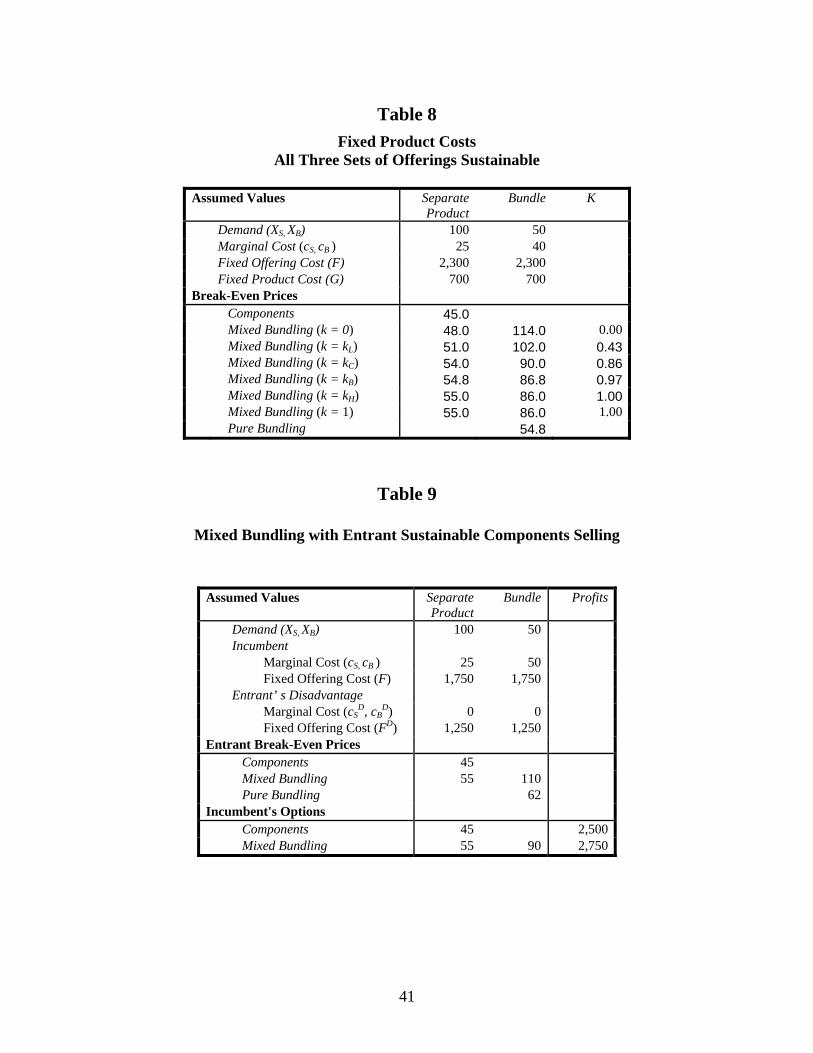
Table 8 Fixed Product Costs

All Three Sets of Offerings Sustainable

Assumed Values Separate Product

Bundle K

Demand (XS, XB) 100 50 Marginal Cost (cS, cB ) 25 40 Fixed Offering Cost (F) 2,300 2,300 Fixed Product Cost (G) 700 700

Break-Even Prices Components 45.0 Mixed Bundling (k = 0) 48.0 114.0 0.00 Mixed Bundling (k = kL) 51.0 102.0 0.43 Mixed Bundling (k = kC) 54.0 90.0 0.86 Mixed Bundling (k = kB) 54.8 86.8 0.97 Mixed Bundling (k = kH) 55.0 86.0 1.00 Mixed Bundling (k = 1) 55.0 86.0 1.00 Pure Bundling 54.8

Table 9

Mixed Bundling with Entrant Sustainable Components Selling

Assumed Values Separate Product

Bundle Profits

Demand (XS, XB) 100 50 Incumbent Marginal Cost (cS, cB ) 25 50 Fixed Offering Cost (F) 1,750 1,750 Entrant’ s Disadvantage Marginal Cost (cS

D, cBD) 0 0

Fixed Offering Cost (FD) 1,250 1,250 Entrant Break-Even Prices

Components 45 Mixed Bundling 55 110 Pure Bundling 62

Incumbent's Options Components 45 2,500 Mixed Bundling 55 90 2,750

41

Table 10

Components Selling With Entrant Sustainable Pure Bundling

Good (i)

Profits

Assumed Values 1 2 Bundle Demand (Xi) 100 100 50 Incumbent Marginal Cost (ci) 25 25 35 Fixed Offering Cost (F) 1,750 1,750 1,750 Entrant’ s Disadvantage Marginal Cost (ci

D) 0 0 0 Fixed Offering Cost (FD) 2,750 2,750 2,750

Entrant Break-Even Prices Components 55 55 Mixed Bundling 70 70 125 Pure Bundling 53

Incumbent's Options Components 53 55 5,200 Mixed Bundling 53 55 108 4,200 Pure Bundling 53 2,750

42

Table 11

Pure Bundling with Entrant Sustainable Mixed Bundling

Assumed Values Separate Product

Bundle Profits

Demand (XS, XB) 100 100 Incumbent Marginal Cost (cS, cB ) 10 18 Fixed Offering Cost (F) 3,000 3,000 Entrant’ s Disadvantage Marginal Cost (cS

D, cBD) 15 30

Fixed Offering Cost (FD) 0 0 Entrant Break-Even Prices

Components 40 Mixed Bundling 55 78 Pure Bundling 58

Incumbent's Options Mixed Bundling 55 78 6,000 Pure 55 8,100

43

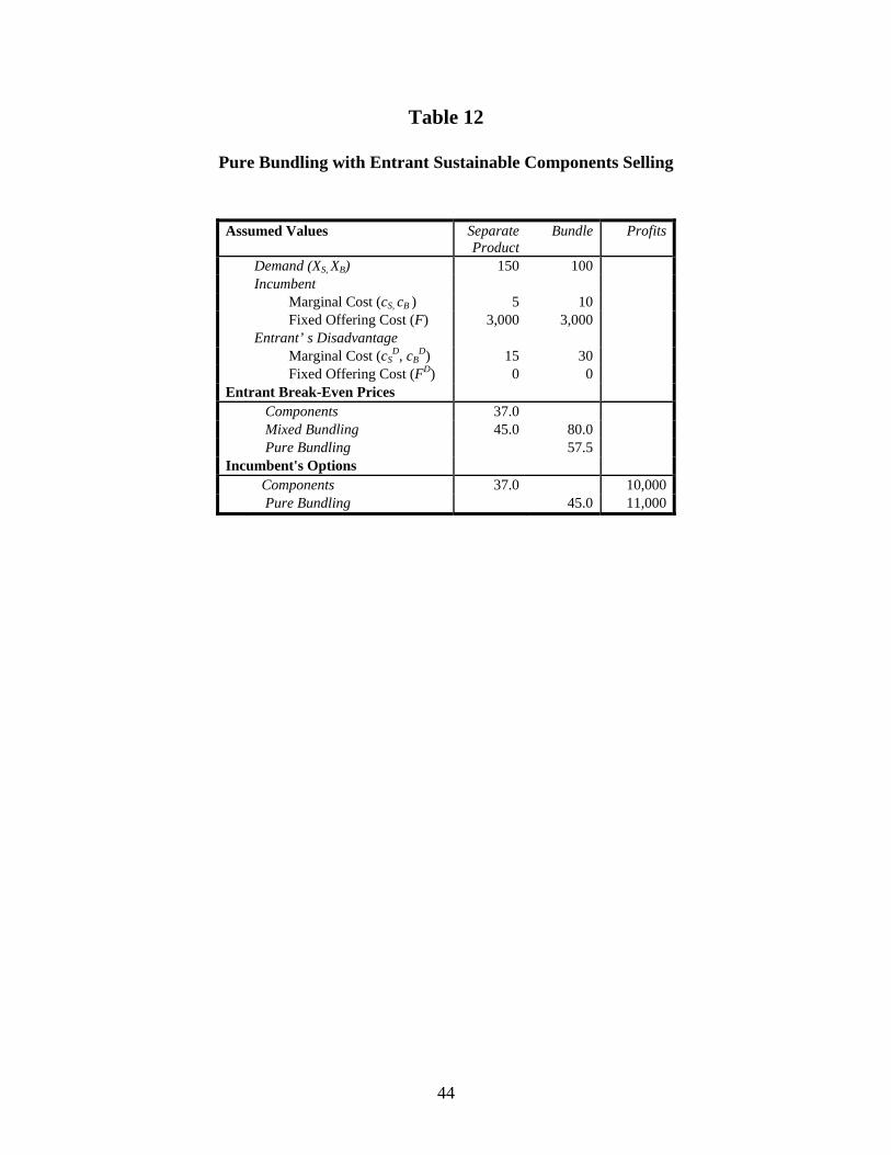
44

Table 12

Pure Bundling with Entrant Sustainable Components Selling

Assumed Values Separate Product

Bundle Profits

Demand (XS, XB) 150 100 Incumbent Marginal Cost (cS, cB ) 5 10 Fixed Offering Cost (F) 3,000 3,000 Entrant’ s Disadvantage Marginal Cost (cS

D, cBD) 15 30

Fixed Offering Cost (FD) 0 0 Entrant Break-Even Prices

Components 37.0 Mixed Bundling 45.0 80.0 Pure Bundling 57.5

Incumbent's Options Components 37.0 10,000 Pure Bundling 45.0 11,000