TWO-WAY CONTINGENCY TABLESWITH MARGINALLY AND

CONDITIONALLY IMPUTEDNONRESPONDENTS

By

Hansheng Wang

A dissertation submitted in partial fulfillment of the

requirements for the degree of

Doctor of Philosophy

(Statistics)

at the

UNIVERSITY OF WISCONSIN – MADISON

2006

i

Abstract

We consider estimating the cell probabilities and testing hypotheses in a two-way

contingency table where two-dimensional categorical data have nonrespondents

imputed using either conditional imputation or marginal imputation. Under

simple random sampling, we derive asymptotic distributions for cell probability

estimators based on the imputed data. Under conditional imputation, we also

show that these estimators are more efficient than those obtained by ignoring

nonrespondents when the proportion of nonrespondents is large. A Wald type

test along with a Rao and Scott type corrected chi-square test for goodness-

of-fit are derived. We show that the naive chi-square test for independence,

which treats imputed values as observed data, is still asymptotically valid under

marginal imputation. Provided we make a simple adjustment of multiplying by

an appropriate factor, the naive chi-square test for independence is also valid

under conditional imputation. We present simulation results which examine the

size and compare the power of these tests. Some of the results are extended

to stratified sampling with imputation within each stratum or across strata.

Asymptotics are studied under two types of stratified sampling: 1) when the

number of strata is fixed with large stratum sizes and 2) when the number of

strata is large with small stratum sizes.

ii

Acknowledgements

First, I want to express my deepest gratitude to my PH.D. adviser Prof. Jun

Shao. It is him who suggested my thesis topic and led me into the field of sample

survey and imputation. For the first time in my life, I found that the world of

statistics is so exciting! My curiosities, enthusiasms, and ambitions are always

encouraged and appreciated there. It is his endless help and encourage that

makes my academic life in Madison so challenging and productive. Prof. Shao

also helps me build up my own research style, which emphasize both theories

and application. It is also Prof. Shao who introduces me to Dr. Shein-Chung

Chow, another respected researcher I am so grateful to.

Although Dr. Chow did not give me help on sample survey and imputation,

it is him who led me into the field of pharmaceutical statistics, where I believe

I am going to build up my own career. The most important thing I learned

from Dr. Chow is “practical sense”, which gives me a unique understanding of

what is statistics and what statistics should do. Statistics is neither science nor

mathematics. Instead, it is a way of reasoning and a philosophy of understand-

ing, when unexplained variation exists in the data. I believe this understanding

will play an important role in guiding my future career and research.

Next, I want to thanks all my friends for their help and support. I want to

thanks Landon Sego, David Dahl, Emmily Chow, and JoAnne Pinto for their

iii

careful proofing of my thesis. Without their help, I can not finish my thesis

writing in such a short time. I also want to thanks Bing Chen, Quan Hong, and

Yuefeng Lu for their help and support when I was defending my thesis in Madi-

son. I also want to thanks my college classmates Xuan Liu and Xiaohuang Hong

for their long-time support and encourage since college whenever I encounter

difficulty.

Furthermore, I want to thanks my PH.D. defense committee, which includes

Prof. Richard Johnson, Prof. Kam-Wah Tsui, Prof. Yi Lin, and Prof. Jun

Zhu, for their careful reading and constructive comments.

Finally, I want to give special thanks to my parents. As the only child of

the family, I was given all the love, bless, and wishes they can give. They are

my support and motivation whenever I want to give up. During the past three

years’ study in USA, I missed them so much. I wish my PH.D. degree can bring

them happiness and proud!!

iv

Contents

Abstract i

Acknowledgements ii

1 Introduction 1

1.1 Background . . . . . . . . . . . . . . . . . . . . . . . . . . . . . 1

1.2 An Outline . . . . . . . . . . . . . . . . . . . . . . . . . . . . . 4

2 Imputation Under Simple Random Sampling 6

2.1 Introduction . . . . . . . . . . . . . . . . . . . . . . . . . . . . . 6

2.1.1 Statistical Model for Nonresponse . . . . . . . . . . . . . 7

2.2 Marginal and Conditional Imputation . . . . . . . . . . . . . . . 8

2.3 Asymptotic Distribution . . . . . . . . . . . . . . . . . . . . . . 11

2.3.1 The Case Where A and B Are Independent . . . . . . . 12

2.3.2 The Case Where A and B Are Dependent . . . . . . . . 21

2.4 Weighted Mean Squared Error . . . . . . . . . . . . . . . . . . . 23

2.5 Testing for Goodness-of-Fit . . . . . . . . . . . . . . . . . . . . 27

2.6 Testing for Independence . . . . . . . . . . . . . . . . . . . . . . 28

3 Simulation Study Under Simple Random Sampling 32

3.1 Introduction . . . . . . . . . . . . . . . . . . . . . . . . . . . . . 32

v

3.2 Asymptotic Normality . . . . . . . . . . . . . . . . . . . . . . . 33

3.3 Weighted Mean Squared Error . . . . . . . . . . . . . . . . . . . 34

3.4 Testing for Goodness-of-Fit . . . . . . . . . . . . . . . . . . . . 35

3.5 Testing for Independence . . . . . . . . . . . . . . . . . . . . . . 36

3.5.1 Marginal Imputation . . . . . . . . . . . . . . . . . . . . 36

3.5.2 Conditional Imputation . . . . . . . . . . . . . . . . . . 36

3.5.3 Relative Efficiency . . . . . . . . . . . . . . . . . . . . . 37

3.6 Conclusion . . . . . . . . . . . . . . . . . . . . . . . . . . . . . . 40

4 Imputation Under Stratified Sampling 57

4.1 Introduction . . . . . . . . . . . . . . . . . . . . . . . . . . . . . 57

4.2 Imputation Within Each Stratum . . . . . . . . . . . . . . . . . 58

4.2.1 Asymptotic Distribution . . . . . . . . . . . . . . . . . . 58

4.2.2 Rao’s Test for Goodness-of-Fit . . . . . . . . . . . . . . . 61

4.3 Imputation Across Strata with Small H . . . . . . . . . . . . . . 62

4.3.1 Asymptotic Distribution . . . . . . . . . . . . . . . . . . 63

4.3.2 Rao’s Test for Goodness-of-fit . . . . . . . . . . . . . . . 68

4.4 Imputation Across Strata with Large H . . . . . . . . . . . . . . 69

4.4.1 Asymptotic Distribution . . . . . . . . . . . . . . . . . . 70

4.4.2 Asymptotic Covariance and Estimation . . . . . . . . . . 76

5 Simulation Study Under Stratified Sampling 84

5.1 Introduction . . . . . . . . . . . . . . . . . . . . . . . . . . . . . 84

vi

5.2 Imputation Within Each Stratum . . . . . . . . . . . . . . . . . 85

5.2.1 Wald’s Test for Goodness-of-Fit . . . . . . . . . . . . . . 85

5.2.2 Rao’s Test for Goodness-of-Fit . . . . . . . . . . . . . . . 86

5.3 Imputation Across Strata with Small H . . . . . . . . . . . . . . 86

5.3.1 Wald’s Test for Goodness-of-Fit . . . . . . . . . . . . . . 86

5.3.2 Rao’s Test for Goodness-of-Fit . . . . . . . . . . . . . . . 87

5.4 Imputation Across Strata with Large H . . . . . . . . . . . . . . 87

5.5 Conclusion . . . . . . . . . . . . . . . . . . . . . . . . . . . . . . 88

6 Real Data Study 104

6.1 The Beaver Dam Eye Study . . . . . . . . . . . . . . . . . . . . 104

6.2 Victimization Incidents Study . . . . . . . . . . . . . . . . . . . 106

Bibliography 111

1

Chapter 1

Introduction

1.1 Background

Two-way contingency tables are widely used for summarizing two dimensional

categorical data. Each cell in a two-way contingency table is a category de-

fined by two-dimensional categorical variables. Sample cell frequencies are often

computed based on the observed responses (of the two-dimensional categorical

variables) from a sample of units (subjects). Statistical inferences including es-

timating cell probabilities, testing the hypothesis of independence, and testing

goodness-of-fit are often carried out.

In sample surveys or medical studies, it is not uncommon for one or two of the

categorical responses to be missing. Sampled units for which both components

are missing (unit nonrespondents) can be handled by a suitable adjustment of

sampling weights. In practice, however, many sampled units may have exactly

one missing component in their responses (item nonrespondents). The approach

of ignoring data from sampled units with exactly one missing component is not

acceptable, because throwing away the observed data may result in a serious

decrease in efficiency of the analysis.

2

A popular method to handle item nonresponses is imputation, which inserts

values for the unobserved items. Justification for the use of imputation with

practical considerations can be found in Kalton and Kasprzyk (1986). After im-

putation, statistical inferences can then be made by treating the imputed values

as the observed data using formulas designed for the case of no nonresponse.

Various imputation methods have been proposed and studied by different

authors (Little and Rubin, 1987; Schafer, 1997). All the imputation methods

can be roughly divided into two categories: model based imputation methods

and nonparametric imputation methods. The model based imputation methods

assume a parametric or semi-parametric model for the responses and the miss-

ingness. The most typical example is regression imputation, which assumes a

linear model between the response and the observed covariates. The situation

where the random errors in the linear model are normally distributed was stud-

ied by Srivastava and Carter (1986). Shao and Wang (2001) extend the results

to include the case in which there was no parametric assumption for the random

error. The nonparametric imputation methods do not make any parametric as-

sumption on the distribution of responses and missingness. Typical approaches

belonging to this category include hot deck imputation, cold deck imputation,

and nearest neighborhood imputation (Chen and Shao 2000; Chen and Shao,

2001).

However, all the above methods investigate either continuous data or one-

dimensional categorical data. The imputation methods for multi-dimensional

3

categorical data are not well studied. For example, for a two-way contingency

table, which is essentially a multi-dimensional categorical data problem, the

statistical problems of interest include the following: How dose one impute

the data? How does the relative efficiency of imputation compare with other

methods, (e.g. re-weighting method)? How can tests be performed in a valid

way?

Another important problem for imputation is the variance/covariance esti-

mation. It is well known that the variance/covariance of the estimators given

by imputation may be different from the variance/covariance of the estimators

for complete data sets. As a result, the estimators designed to estimate the

variance and covariance of estimators for complete data sets may not be valid

for the estimators generated by imputation. There are three commonly used

approaches to obtain estimators for the variance and covariance of estimators

given by imputation. One is linearization, which uses Taylor’s expansion to ob-

tain an explicit theoretical formula for the covariance structure of the estimators

and then replace all the unknown quantities by their consistent point estima-

tors. The merit of the linearization method is that it requires less computation

as compared with other methods, e.g., resampling methods. However, it is not

uncommon that the theoretical formula is too complex to be used. As an al-

ternative, resampling methods such as jackknife and bootstrap (Rao and Shao,

1992) are commonly used to obtain the variance/covariance estimators. The

third approach is multiple imputation (Rubin, 1987), which imputes the same

4

data set more than once and then obtains the variance estimator by combining

the between and within imputation variability in an appropriate way.

The main purpose of this thesis is to investigate the statistical properties of

a conditional imputation method, which imputes nonrespondents using the esti-

mated conditional probabilities. More specifically, we study (i) the consistency

of estimators of cell probabilities based on imputed data; (ii) the asymptotic

variances and covariances of estimators of cell probabilities, which lead to con-

sistent variance and covariance estimators; and (iii) the validity of chi-square

type tests for goodness of fit or independence. For testing independence of

the two components of the categorical variable, we also study a marginal im-

putation method, which imputes nonrespondents using the estimated marginal

probabilities.

1.2 An Outline

The rest of this thesis is organized as follows. In Chapter 2, we study both con-

ditional and marginal imputation under simple random sampling. In Chapter 3,

extensive simulations are performed to evaluate the finite sample performance

of the procedures described in Chapter 2. In Chapter 4, we study conditional

imputation for stratified sampling, which includes imputation within stratum

and imputation across strata. For the method of imputation across strata, two

different types of asymptotics are considered. One deals with a small num-

ber of strata with a large stratum size. The other is a large number of strata

5

with a small stratum size. Extensive simulations are carried out in Chapter 5

to evaluate the finite sample performance of the procedures obtained in Chap-

ter 4. Finally, several real data sets are presented to illustrate the proposed

imputation methods in Chapter 6.

6

Chapter 2

Imputation Under Simple

Random Sampling

2.1 Introduction

In this chapter, we introduce two imputation methods under simple random

sampling: marginal imputation and conditional imputation. Our results show

that the point estimators obtained by conditional imputation are consistent,

but those obtained by marginal imputation are usually not unless the two

components of the categorical variables are independent of each other. The

asymptotic distributions of point estimators under both imputation methods

are derived when appropriate. In order to evaluate the statistical performances

of the point estimators, we propose a measure called Weighted Mean Squared

Error (WMSE). Then the estimators given by conditional imputation and re-

weighting methods are compared in terms of WMSE. The results show that

conditional imputation can improve efficiency when the proportion of complete

units is small. Testing goodness-of-fit is also considered. We first propose a

7

Wald type statistic, which is asymptotically valid. Then we show that perform-

ing the naive method of treating the imputed value as observed and applying

Pearson’s chi-square test is not valid. We propose a Rao type correction to the

naive method. Finally, the performances of Wald type statistic and Rao type

statistic are compared. Results show that their performances are comparable

in terms of type I error. Testing independence is also considered. We show

that the naive method of applying Pearson’s chi-square statistic directly is still

asymptotically valid under marginal imputation but not under conditional im-

putation. By simply fixing a constant, the naive method is also asymptotically

correct under conditional imputation.

2.1.1 Statistical Model for Nonresponse

Consider a two-dimensional response vector (A,B)′, where both A and B are

categorical responses taking values from {1, · · · , a} and {1, · · · , b}, respectively.

In practice, imputation is carried out by first creating some imputation

classes and imputing nonrespondents within each imputation class. Imputation

classes are sub-populations of the original population and are usually formed by

using an auxiliary variable without nonresponse. For example, in many business

surveys, imputation classes are strata or unions of strata. In medical studies, if

data are obtained under several different treatments, the treatment groups are

imputation classes.

Throughout this chapter, we make the following assumption:

8

Assumption A. For each sampled unit within an imputation class, πA de-

notes the probability of observing A and missing B, πB denotes the probability

of observing B and missing A, and πC denotes the probability of observing both

A and B.

As discussed in the previous chapter, the units with both respondents miss-

ing (unit nonresponses) can be ignored by suitably adjusting the sampling

weights. As a result, we assume there is no unit nonresponse, i.e., πA+πB+πC =

1. Note that the probability πA, πB, and πC may be different in different impu-

tation classes.

For simplicity and without loss of generality, we only consider the case of

simple random sampling with replacement. In practice, the data may be ob-

tained by sampling without replacement. Our derived results are still valid if

the sampling fraction is negligible.

For the sake of convenience, we assume that there is only one imputation

class, since the extension to multiple imputation classes is straightforward.

2.2 Marginal and Conditional Imputation

Suppose there are n sampled units, which are indexed by k (i.e., (Ak, Bk), k =

1, · · · , n). To simplify the notation, (Ak, Bk) may also be referred to as (A,B).

Let CA, CB, and CC be the collection of the indices of the units with B missing,

A missing, and neither A nor B missing, respectively. Let nA = |CA|, nB = |CB|,

9

and nC = |CC |, where |S| denotes the number of elements contained in a finite

set S. In other words, nA, nB, and nC are the number of the units with B

missing, with A missing, and neither A nor B missing, respectively. Therefore,

the total sample size is given by n = nA + nB + nC . Let nCij denote the total

number of completers such that (A,B) = (i, j). Let pij = P ((A,B) = (i, j)),

pi· = P (A = i), and p·j = P (B = j). A typical method for estimation of pi· and

p·j can be obtained by using completers as follows

pCi· =

∑bj=1 nC

ij∑ij nC

ij

=nC

i·nC

and

pC·j =

∑ai=1 nC

ij∑ij nC

ij

=nC·j

nC,

where nCi· =

∑bj=1 nC

ij, nC·j =

∑ai=1 nC

ij, and nC =∑

ij nCij.

Given an incompleter (A,B) = (i, ∗), where * denotes the missing value,

marginal imputation imputes the missing value j (1 ≤ j ≤ b) with probabil-

ity pC·j . It means that the missing value is imputed according to its estimated

marginal distribution without conditioning on the observed item (A = i). Miss-

ing values from incompleters are imputed independently. Intuitively, parameters

such as p·j and pi· can be estimated consistently based on marginally imputed

data, but parameters such as pij cannot be estimated consistently, since the

relationship between A and B is not preserved during marginal imputation.

The conditional probability P (B = j|A = i) is denoted by pij|A = pij/pi·.

10

Thus, an estimator based on completers for pij|A is given by

pCij|A =

pCij

pCi·

=nC

ij/nC

nCi· /nC

=nC

ij

nCi·

.

Conditional imputation imputes the missing value j (1 ≤ j ≤ b) with probability

pCij|A. In other words, given the completers, conditional imputation imputes

a missing value according to its estimated conditional distribution given the

observed component. Imputation for an incompleter with A missing is similar,

and incompleters are imputed independently, conditioning on the completers

and their observed components.

After imputation, estimators of pij are obtained using the standard formulas

in a two-way contingency table by treating the imputed values as observed

data. We denote those estimators (based on either marginal or conditional

imputation) by pIij.

Recall that CA is the collection of the indices of the units with A observed

and B missing. Let

pAij =

1

nA

∑

k∈CA

I{(Ak, Bk) = (i, j)},

where Bk is the value obtained by imputation (either marginal imputation or

conditional imputation) for any k ∈ CA. pBij and pC

ij are similarly defined. The

relationship between pIij and pA

ij, pBij, pC

ij is given by

pIij =

nApAij + nB pB

ij + nC pCij

n.

11

For the sake of convenience, we define

p = (p11, · · · , p1b, · · · , pa1, · · · , pab)′

pA = (p1·, · · · , pa·)′

pB = (p·1, · · · , p·b)′

pI = (pI11, · · · , pI

1b, · · · , pIa1, · · · , pI

ab)′

pA = (pA11, · · · , pA

1b, · · · , pAa1, · · · , pA

ab)′

pB = (pB11, · · · , pB

1b, · · · , pBa1, · · · , pB

ab)′

pC = (pC11, · · · , pC

1b, · · · , pCa1, · · · , pC

ab)′.

(2.1)

2.3 Asymptotic Distribution

In order to obtain the limiting distribution of pIij, Lemma 1 is given here without

proof. Lemma 1 is also used when we study stratified sampling in Chapter 4.

A more general form of the lemma can be found in Schenker and Welsh (1988).

Lemma 1 Let Xn be a sample, and Un(Xn), Wn be two random vectors, such

that

Un →d N(0, Σ1)

and

Wn|Xn →d N(0, Σ2),

then

Un + Wn →d N(0, Σ1 + Σ2).

12

2.3.1 The Case Where A and B Are Independent

When A and B are independent, the estimators produced by both marginal and

conditional imputation are consistent. However, their variances and covariances

are different from the variances and covariances of the standard estimator of pij

when there is no nonresponse. The following theorem establishes the asymptotic

distributions and covariance matrices of pI , which were defined in (2.1), under

both conditional imputation and marginal imputation.

Theorem 1 Assume that A and B are independent. If πC > 0, then, as n →∞,

√n(pI − p) →d N(0, Σ),

where

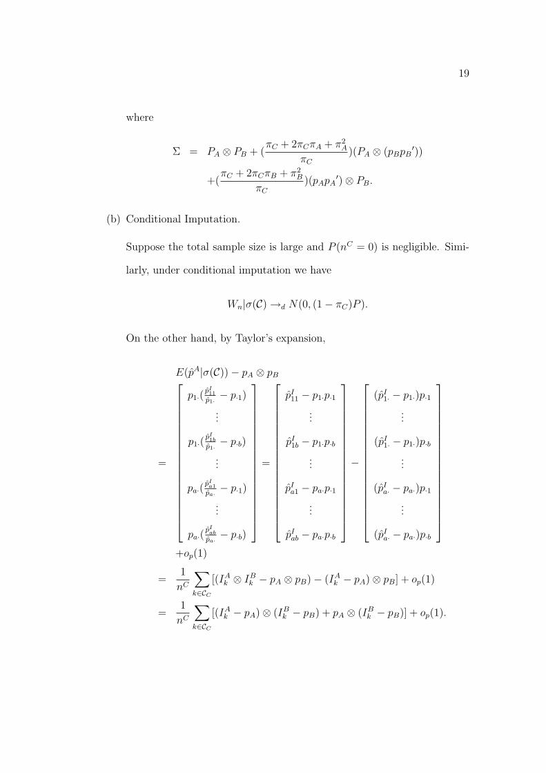
(a) under marginal imputation

Σ = PA ⊗ PB + (πC+2πCπA+π2

A

πC)(PA ⊗ (pBpB

′))

+(πC+2πCπB+π2

B

πC)(pApA

′)⊗ PB;

(b) under conditional imputation

Σ = ( 1πC

+ 1− πC)PA ⊗ PB + (πC+2πCπA+π2

A

πC)(PA ⊗ (pBpB

′))

+(πC+2πCπB+π2

B

πC)(pApA

′)⊗ PB.

⊗ is the Kronecker product; pA and pB are given in (2.1). PA = diag(pA)−pAp′A,

where diag(pA) denotes a diagonal matrix with the same dimension as pA and

with its ith (1 ≤ i ≤ a) diagonal element to be the ith component of pA.

13

PB = diag(pB)− pBp′B.

Proof:

After imputation, each unit becomes “complete”. For a given unit, (Ak, Bk),

we can define IAk to be an a-dimensional vector with the ith element equal to 1

and the others equal to 0 if Ak = i. Similarly, define IBk to be a b-dimensional

vector with jth element equal to 1 and the others equal to 0 if Bk = j. Under

the hypothesis that A and B are independent, IAk and IB

k are independent.

According to (2.1), note that

pI =1

n

n∑t=1

IAk ⊗ IB

k

pA =1

nA

∑t∈CA

IAk ⊗ IB

k

pB =1

nB

∑t∈CB

IAk ⊗ IB

k

pC =1

nC

∑t∈CC

IAk ⊗ IB

k .

It follows that

√n(pI − p)

=√

n

[nA(pA − p) + nB(pB − p) + (pC − p)

n

]

=√

n

[nA(E(pA|σ(C))− p) + nB(E(pB|σ(C))− p) + nC(pC − p)

n

]

14

+√

n

[nA(pA − E(pA|σ(C))) + nB(pB − E(pB|σ(C)))

n

],

where E(·|σ(C)) denotes E(·|nA, nB, nC , (Ak, Bk), k ∈ CA). In other words,

E(·|σ(C)) denotes the expectation conditional on the completers and the number

of incompleters. Let

Un =√

n

[nA(E(pA|σ(C))− p) + nB(E(pB|σ(C))− p) + nC(pC − p)

n

], (2.2)

and

Wn =√

n

[nA(pA − E(pA|σ(C))) + nB(pB − E(pB|σ(C)))

n

]. (2.3)

(a) Marginal imputation.

Given σ(C) (i.e., nA, nB, nC , and the completers), {IAk ⊗ IB

k }k∈CAare i.i.d

random vector with mean E(pA|σ(C)). According to Central Limit Theo-

rem,√

nA(pA − E(pA|σ(C)))|σ(C) →d N(0, ΣW ),

and

ΣW = diag{E(pA|σ(C))} − (E(pA|σ(C)))(E(pA|σ(C)))′.

On the other hand,

E(pAij|σ(C)) = pi·pC

·j →a.s pi·p·j = pij as nC →∞.

Therefore,

ΣW →a.s diag{p} − pp′ .= P, (2.4)

15

where “.=” denotes “defined to be”. This leads to Wn|σ(C) →d N(0, P ).

Consequently,

Wn|σ(C)

=

√nA

n

√nA(pA − E(pA|σ(C)))

+

√nB

n

√nB(pB − E(pB|σ(C)))

=√

πA

√nA(pA − E(pA|σ(C)))

+√

πB

√nB(pB − E(pB|σ(C))) + op(1)

→d

√πAN(0, P ) +

√πBN(0, P ) = N(0, (1− πC)P ).

Under the assumption that A and B are independent, it follows that

E[pA|σ(C)]− p =

p1·pC·1 − p11

...

p1·pC·b − p1b

...

pa·pC·1 − pa1

...

pa·pC·b − pab

=

p1·(pC·1 − p·1)

...

p1·(pC·b − p·b)

...

pa·(pC·1 − p·1)

...

pa·(pC·b − p·b)

= pA ⊗ [1

nC

∑

k∈CC

(IBk − pB)]

=1

nC

∑

k∈CC

pA ⊗ (IBk − pB).

16

Similarly,

E(pB|σ(C))− p =1

nC

∑(IA

k − pA)⊗ PB.

Thus, we have

Un

=1√n

[nA(E(pA|σ(C))− p) + nB(E(pB|σ(C))− p) + nC(pC − p)

]

=nA

√nnC

√nC(E(pA|σ(C))− p) +

nB

√nnC

√nC(E(pB|σ(C))− p)

+

√nC

n

√nC(pC − p)

=πA√πC

√nC(E(pA|σ(C)− p)

+πB√πC

√nC(E(pB|σ(C)− p)

+√

πC

√nC(pC − p) + op(1)

=1√nC

∑

k∈CC

[√πC(IA

k − pA)⊗ (IBk − pB) +

πC + πA√πC

pA ⊗ (IBk − pB)

+πC + πB√

πC

(IAk − pA)⊗ pB

]+ op(1)

→d N(0, ΣU),

where

ΣU = var

(√πC(IA

k − pA)⊗ (IBk − pB) +

πC + πA√πC

pA ⊗ (IBk − pB)

+πC + πB√

πC

(IAk − pA)⊗ pB

).

17

Let PA = diag{pA} − pApA′ and PB = diag{pB} − pBpB

′. Then we have

var[(IAk − pa)⊗ (IB

k − pB)]

= E{[(IAk − pA)⊗ (IB

k − pB)][(IAk − pA)⊗ (IB

k − pB)]′}

= E{[(IAk − pA)(IA

k − pA)′]⊗ [(IBk − pB)(IB

k − pB)′]}

= E[(IAk − pA)(IA

k − pA)′]⊗ E[(IBk − pB)(IB

k − pB)′]

= PA ⊗ PB.

The third equation holds because IAk and IB

k are independent. Similarly

var[pA ⊗ (IBk − pB)] = (pApA

′)⊗ PB

var[(IAk − pA)⊗ pB] = PA ⊗ (pBpB

′)

cov[(IAk − pA)⊗ (IB

k − pB), pA ⊗ (IBk − pB)]

= E{[(IAk − pA)pA

′]

⊗[(IBk − pB)(IB

k − pB)′]}

= 0⊗ PB = 0

cov[(IAk − pA)⊗ (IB

k − pB), (IAk − pA)⊗ pB]

= E{[(IAk − pA)(IA

k − pA)′]

⊗[(IBk − pB)pB

′]

= PA ⊗ 0 = 0

18

cov[pA ⊗ (IBk − pB), (IA

k − pA)⊗ pB]

= E{[pA(IAk − pA)′]

⊗[(IBk − pB)pB

′]}

= 0.

As a result, ΣU is given by

ΣU = πCPA ⊗ PB +(πC + πA)2

πC

(pApA′)⊗ PB +

(πC + πB)2

πC

PA ⊗ (pBpB′).

Therefore, Un →d N(0, ΣU). Since Wn →d N(0, (1− πC)P ) and

P = diag{p} − pp′

= diag{pA ⊗ pB} − (pApA′)⊗ (pBpB

′)

= (diag{pA} − pApA′)⊗ (diag{pB} − pBpB

′)

+(pApA′)⊗ (diag{pB} − pBpB

′)

+(diag{pA} − (pApA′)⊗ (pBpB

′)

= PA ⊗ PB + (pApA′)⊗ PB + PA ⊗ (pBpB

′),

we have

√n(p− p) = Wn + Un

→d N(0, (1− πC)P + ΣU)

= N(0, Σ),

19

where

Σ = PA ⊗ PB + (πC + 2πCπA + π2

A

πC

)(PA ⊗ (pBpB′))

+(πC + 2πCπB + π2

B

πC

)(pApA′)⊗ PB.

(b) Conditional Imputation.

Suppose the total sample size is large and P (nC = 0) is negligible. Simi-

larly, under conditional imputation we have

Wn|σ(C) →d N(0, (1− πC)P ).

On the other hand, by Taylor’s expansion,

E(pA|σ(C))− pA ⊗ pB

=

p1·(pI11

p1·− p·1)

...

p1·(pI1b

p1·− p·b)

...

pa·(pI

a1

pa·− p·1)

...

pa·(pI

ab

pa·− p·b)

=

pI11 − p1·p·1

...

pI1b − p1·p·b

...

pIa1 − pa·p·1

...

pIab − pa·p·b

−

(pI1· − p1·)p·1

...

(pI1· − p1·)p·b

...

(pIa· − pa·)p·1

...

(pIa· − pa·)p·b

+op(1)

=1

nC

∑

k∈CC

[(IAk ⊗ IB

k − pA ⊗ pB)− (IAk − pA)⊗ pB] + op(1)

=1

nC

∑

k∈CC

[(IAk − pA)⊗ (IB

k − pB) + pA ⊗ (IBk − pB)] + op(1).

20

Similarly,

E(pB|σ(C))− pA ⊗ pB

=1

nC

∑

k∈CC

[(IAk − pA)⊗ (IB

k − pB) + (IAk − pA)⊗ pB] + op(1).

As a result,

Un =1√nC

[√πC(IA

k ⊗ IBk − pA ⊗ pB)

+πA√πC

((IAk − pA)⊗ (IB

k − pB) + pA ⊗ (IBk − pB))

+πB√πC

((IAk − pA)⊗ (IB

k − pB) + (IAk − pA)⊗ pB)

]+ op(1)

=1√nC

∑[1√πC

(IAk − pA)⊗ (IB

k − pB)

+πC + πA√

πC

pA ⊗ (IBk − pB)

+πC + πB√

πC

(IAk − pA)⊗ pB

]+ op(1)

→d N

(0,

1

πC

PA ⊗ PB +(πC + πA)2

πC

(pApA′)⊗ PB

+(πC + πB)2

πC

PA ⊗ (pBpB′))

.

Consequently,

Wn + Un →d N(0, Σ),

where

Σ = (1

πC

+ 1− πC)PA ⊗ PB +πC + 2πCπA + π2

A

πC

(pApA′)⊗ PB

+πC + 2πCπB + π2

B

πC

PA ⊗ (pBpB′).

21

2.3.2 The Case Where A and B Are Dependent

When A and B are dependent, the point estimators obtained by marginal im-

putation are not consistent. Therefore, marginal imputation is usually not con-

sidered in this case. The asymptotic results are established for conditional

imputation only.

Theorem 2 Assume that πC > 0. Under conditional imputation,

√n(pI − p) →d N(0, Σ),

where Σ = MPM ′ + (1− πC)P ,

M =1√πC

Ia×b − πA√πC

diag{pB|A}Ia ⊗ Ub − πB√πC

diag{pA|B}Ua ⊗ Ib, (2.5)

and

pA|B = (p11/p·1, · · · , p1b/p·b, · · · , pa1/p·1, · · · , pab/p·b)′,

pB|A = (p11/p1·, · · · , p1b/p1·, · · · , pa1/pa·, · · · , pab/pa·)′.(2.6)

Id (d = a × b, a, or b) is a d-dimensional identity matrix, and Ud is a d-

dimensional square matrix with all elements equal to 1.

Proof:

Un and Wn are defined in (2.2) and (2.3). Under conditional imputation, we

have

Wn|σ(C) →d N(0, (1− πC)P ),

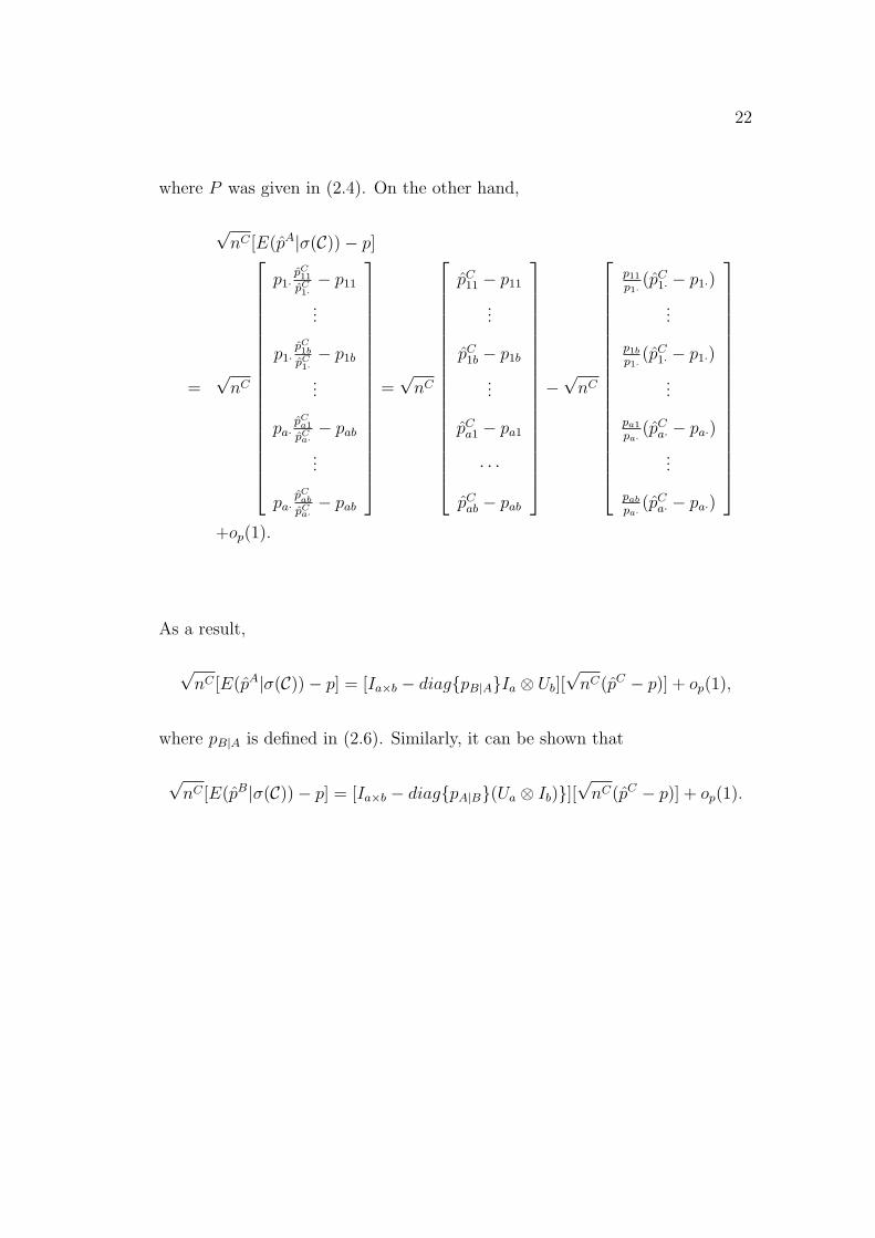
22

where P was given in (2.4). On the other hand,

√nC [E(pA|σ(C))− p]

=√

nC

p1·pC11

pC1·− p11

...

p1·pC1b

pC1·− p1b

...

pa·pC

a1

pCa·− pab

...

pa·pC

ab

pCa·− pab

=√

nC

pC11 − p11

...

pC1b − p1b

...

pCa1 − pa1

· · ·pC

ab − pab

−√

nC

p11

p1·(pC

1· − p1·)

...

p1b

p1·(pC

1· − p1·)

...

pa1

pa·(pC

a· − pa·)

...

pab

pa·(pC

a· − pa·)

+op(1).

As a result,

√nC [E(pA|σ(C))− p] = [Ia×b − diag{pB|A}Ia ⊗ Ub][

√nC(pC − p)] + op(1),

where pB|A is defined in (2.6). Similarly, it can be shown that

√nC [E(pB|σ(C))− p] = [Ia×b − diag{pA|B}(Ua ⊗ Ib)}][

√nC(pC − p)] + op(1).

23

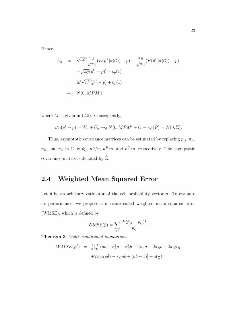
Hence,

Un =√

nC [πA√πC

(E(pA|σ(C))− p) +πB√πC

(E(pB|σ(C))− p)

+√

πC(pC − p)] + op(1)

= M√

nC(pC − p) + op(1)

→d N(0,MPM ′),

where M is given in (2.5). Consequently,

√n(pI − p) = Wn + Un →d N(0,MPM ′ + (1− πC)P ) = N(0, Σ).

Thus, asymptotic covariance matrices can be estimated by replacing pij, πA,

πB, and πC in Σ by pIij, nA/n, nB/n, and nC/n, respectively. The asymptotic

covariance matrix is denoted by Σ.

2.4 Weighted Mean Squared Error

Let p be an arbitrary estimator of the cell probability vector p. To evaluate

its performance, we propose a measure called weighted mean squared error

(WMSE), which is defined by

WMSE(p) =∑ij

E(pij − pij)2

pij

.

Theorem 3 Under conditional imputation,

WMSE(pI) = 1n[ 1πC

(ab + π2Aa + π2

Bb− 2πAa− 2πBb + 2πAπB

+2πAπBδ)− πCab + (ab− 1)] + o( 1n),

24

where δ is a non-centrality parameter given by

δ =∑ (pij − pi·p·j)2

pi·p·j.

Intuitively δ can be interpreted as a measure for the dependency between A and

B. When A and B are independent, δ reaches its smallest possible value 0.

Proof:

It has been shown that√

n(pI − p) = N(0, Σ) + op(1), where Σ is given in

Theorem 2. For the sake of convenience, we define

1/√

p = (1/√

p11, · · · , 1/√

p1b, · · · , 1/√

pa1, · · · , 1/√

pab)′

p2/(pApB) = (p211/(p1·p·1), · · · , p2

1b/(p1·p·b), · · · , p2a1/(pa·p·1), · · · , p2

ab/(pa·p·b))′.

It follows that√

ndiag{1/√p}(pI − p) →d N(0, Σ∗), where

Σ∗ = diag{1/√p} · Σ · diag{1/√p}.

On the other side,

Σ = M · diag{p} ·M ′ + (1− πC) · diag{p} − pp′,

and

tr[diag{1/√p · diag{p} · diag{1/√p}] = a× b

tr[diag{1/√p · pp′} · diag{1/√p}] = 1.

25

As a result, we only need to focus on the evaluation of

tr[diag{1/p} ·M · diag{P} ·M ′ · diag{1/p}].

It can be verified that

a = tr[diag{1/√p} · diag{pB|A} · {Ia ⊗ Ub} · diag{p}·{Ia ⊗ Ub} · diag{pB|A} · diag{1/√p}]

b = tr[diag{1/√p} · diag{pA|B} · (Ua ⊗ Ib) · diag{p}·(Ua ⊗ Ib) · diag{pA|B} · diag{1/√p}]

a = tr[diag{1/√p} · diag{p} · (Ia ⊗ Ub) · diag{pB|A}·diag{1/√p}]

a = tr[diag{1/√p} · diag{pB|A} · (Ia ⊗ Ub)

·diag{p} · diag{1/√p}]b = tr[diag{1/√p} · diag{pA|B} · (Ua ⊗ Ib)

·diag{p} · diag{1/√p}b = tr[diag{1/√p} · diag{p}

·(Ua ⊗ Ib) · diag{pA|B} · diag{1/√p}].

Note that

δ =∑ (pij−pi·p·j)2

pi·p·j

=∑ p2

ij

pi·p·j− 2

∑pij +

∑pi·p·j

=∑ p2

ij

pi·p·j− 1

= tr(diag{p2/(pApB)})− 1,

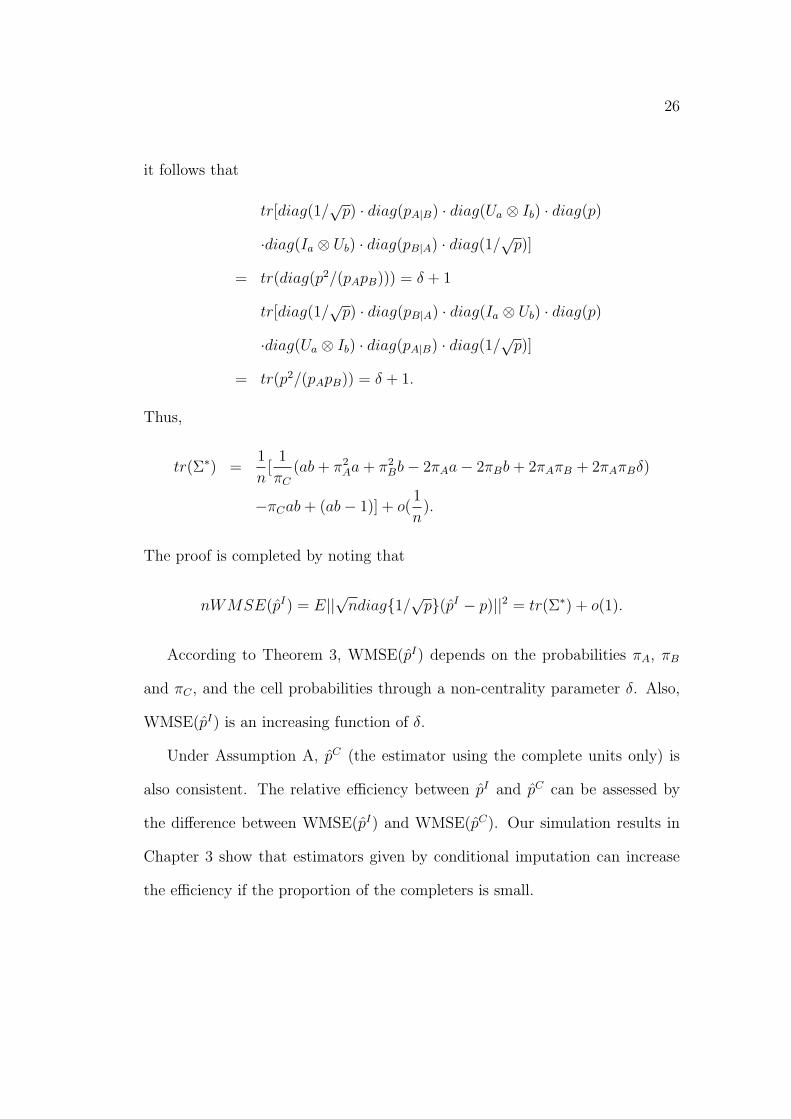
26

it follows that

tr[diag(1/√

p) · diag(pA|B) · diag(Ua ⊗ Ib) · diag(p)

·diag(Ia ⊗ Ub) · diag(pB|A) · diag(1/√

p)]

= tr(diag(p2/(pApB))) = δ + 1

tr[diag(1/√

p) · diag(pB|A) · diag(Ia ⊗ Ub) · diag(p)

·diag(Ua ⊗ Ib) · diag(pA|B) · diag(1/√

p)]

= tr(p2/(pApB)) = δ + 1.

Thus,

tr(Σ∗) =1

n[

1

πC

(ab + π2Aa + π2

Bb− 2πAa− 2πBb + 2πAπB + 2πAπBδ)

−πCab + (ab− 1)] + o(1

n).

The proof is completed by noting that

nWMSE(pI) = E||√ndiag{1/√p}(pI − p)||2 = tr(Σ∗) + o(1).

According to Theorem 3, WMSE(pI) depends on the probabilities πA, πB

and πC , and the cell probabilities through a non-centrality parameter δ. Also,

WMSE(pI) is an increasing function of δ.

Under Assumption A, pC (the estimator using the complete units only) is

also consistent. The relative efficiency between pI and pC can be assessed by

the difference between WMSE(pI) and WMSE(pC). Our simulation results in

Chapter 3 show that estimators given by conditional imputation can increase

the efficiency if the proportion of the completers is small.

27

2.5 Testing for Goodness-of-Fit

A direct application of Theorem 2 is to obtain a Wald type test for goodness-

of-fit. Consider the null hypothesis of H0 : p = p0, where p0 is a known vector.

Under H0,

X2W

.= n(p∗ − p∗0)

′Σ∗−1(p∗ − p∗0) →d χ2ab−1,

where χ2v denotes a chi-square random variable with v degrees of freedom. p∗ (p∗0)

is obtained by dropping the last component of pI (p0) and Σ∗ is the estimated

asymptotic covariance matrix of p∗, which can be obtained by dropping the last

row and column of Σ, the estimated asymptotic covariance matrix of pI .

Although X2W provides an asymptotically correct chi-square test, the compu-

tation of Σ∗−1 is complicated. Instead of looking for an asymptotically correct

test, we consider a simple correction of the standard Pearson’s chi-square statis-

tic by matching the first order moment (Rao and Scott, 1981). When there is

no nonresponse, under H0, the Pearson’s statistic is asymptotically distributed

as a chi-square random variable with ab− 1 degrees of freedom:

X2P = n

∑ (pij − pij)2

pij

→d χ2ab−1. (2.7)

Therefore, E(X2P ) ≈ ab− 1. However, under conditional imputation, it follows

from Theorem 3 that

E(X2P ) ≈ 1

πC

(ab + π2Aa + π2

Bb− 2πAa− 2πBb + 2πAπB + 2πAπBδ)

−πCab + (ab− 1).

28

If we let

λ =1

πC(ab− 1)(ab + π2

Aa + π2Bb− 2πAa− 2πBb + 2πAπB

+2πAπBδ)− πCab

ab− 1+ 1, (2.8)

it follows that E(X2P /λ) ≈ (ab− 1). Thus, we propose the corrected Pearson’s

statistic X2C = X2

P /λ. The performance of this corrected chi-square test, the

naive chi-square test, and Wald’s test are evaluated by a simulation study in

Chapter 3.

2.6 Testing for Independence

An application of Theorem 1 is testing the independence of A and B. When

πC = 1, (i.e., there are no cases of nonresponses) the chi-square statistic is given

by

X2I

.= n

∑(pij − pi·p·j)2

pi·p·j→d χ2

(a−1)(b−1).

The following theorem establishes the asymptotic behavior of X2I under marginal

imputation and conditional imputation when πC > 0.

Theorem 4 Assume that πC > 0 and that A and B are independent.

(a) When marginal imputation is applied to impute nonrespondents,

X2I →d χ2

(a−1)(b−1).

29

(b) When conditional imputation is applied to impute nonrespondents,

X2I /(π−1

C + 1− πC) →d χ2(a−1)(b−1).

Proof:

(a) After marginal imputation, the test statistics given by

X2I = n

∑ (pIij − pI

i·pI·j)

2

pIi·p

I·j

= ||Vn||2,

where Vn is a ab-dimensional vector with

√n(pI

ij − pIi·p

I·j)√

pIi·p

I·j

as its dth component, where d = (i− 1)b + j. By Taylor’s expansion and

Slusky’s theorem,

√n(pI

ij − pIi·p

I·j)√

pIi·p

I·j

=

√n(pI

ij − pIi·p·j − pi·pI

·j + pi·p·j)√pi·p·j

+ op(1).

Define

U = Ia×b − (pA1′a)⊗ Ib − Ia ⊗ (pB1′b),

where 1a and 1b are two vectors with all elements equal to 1 and dimension

a and b, respectively. Let 1/√

pA denote the vector (1/√

p1·, · · · , 1/√

pa·)′,

and let 1/√

pB be defined similarly. Define S = diag{(1/√pA)⊗(1/√

pB)}.Note that

Vn = SU(√

n(pI − p)) + op(1) →d N(0, SUΣU ′S ′),

30

where Σ is given in Theorem 1, which is of the form

κPA ⊗ PB + x(pApA′)⊗ PB + yPA ⊗ (pBpB

′),

where κ = 1/πC + 1− πC under conditional imputation, and κ = 1 under

marginal imputation.

Note that

PA(1pA′) = (pA1′)PA = 0

PB(1pB′) = (pB

′1)PB = 0

(pApA′)(1pA

′) = (pA1′)(pApA′) = (pApA

′)

(pBpB′)(1pB

′) = (pB1′)(pBpB′) = (pBpB

′).

As a result,

UΣU ′ = κPA ⊗ PB.

Since

S = diag{1/√pi·} ⊗ diag{1/√p·j},

it follows that

SUΣU ′S ′ = κP ∗A ⊗ P ∗

B,

where

P ∗A = diag(1/

√pA) · PA · diag(1/

√pA)

= diag(1/√

pA) · (diag{pA} − pApA′) · diag{1/√pA}

= Ia −√pA√

pA′.

31

Similarly,

P ∗B = diag{1/√pB} · PB · diag{1/√pB} = Ib −√pB

√pB

′.

Because both P ∗A and P ∗

B are projection matrices with rank (a − 1) and

(b − 1), respectively, P ∗A ⊗ P ∗

B is also a projection matrix, but with rank

(a− 1)(b− 1). Since

Vn →d N(0, SUΣU ′S ′) = N(0, κP ∗A ⊗ P ∗

B),

it follows that

1

κX2

I = || 1√κVn||2 →d χ2

(a−1)(b−1).

The proof is completed by recalling that under marginal imputation κ = 1

and under conditional imputation κ = 1/πC + 1− πC .

32

Chapter 3

Simulation Study Under Simple

Random Sampling

3.1 Introduction

All the results obtained in the previous chapter are based on large sample the-

ory. In this chapter, extensive simulations are carried out to evaluate the finite

sample performances of the proposed estimators and tests.

In Section 3.2, we study the asymptotic normality through chi-square scores,

which is used by Johnson and Wichern (1998) as a tool to study the normality

of multivariate normal distributions. In Section 3.3 the relative efficiencies of pI

and pC are compared using WMSE. In Section 3.4, two test statistics (Wald type

and Rao type) for goodness-of-fit are compared in terms of size (type I error

probability). In Section 3.5, testing independence under marginal imputation,

conditional imputation, and re-weighting method are studied. Their relative

efficiencies are compared in terms of power.

33

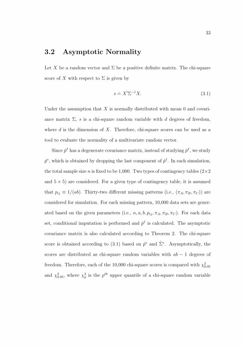
3.2 Asymptotic Normality

Let X be a random vector and Σ be a positive definite matrix. The chi-square

score of X with respect to Σ is given by

s.= X ′Σ−1X. (3.1)

Under the assumption that X is normally distributed with mean 0 and covari-

ance matrix Σ, s is a chi-square random variable with d degrees of freedom,

where d is the dimension of X. Therefore, chi-square scores can be used as a

tool to evaluate the normality of a multivariate random vector.

Since pI has a degenerate covariance matrix, instead of studying pI , we study

p∗, which is obtained by dropping the last component of pI . In each simulation,

the total sample size n is fixed to be 1,000. Two types of contingency tables (2×2

and 5× 5) are considered. For a given type of contingency table, it is assumed

that pij ≡ 1/(ab). Thirty-two different missing patterns (i.e., (πA, πB, πC)) are

considered for simulation. For each missing pattern, 10,000 data sets are gener-

ated based on the given parameters (i.e., n, a, b, pij, πA, πB, πC). For each data

set, conditional imputation is performed and pI is calculated. The asymptotic

covariance matrix is also calculated according to Theorem 2. The chi-square

score is obtained according to (3.1) based on p∗ and Σ∗. Asymptotically, the

scores are distributed as chi-square random variables with ab − 1 degrees of

freedom. Therefore, each of the 10,000 chi-square scores is compared with χ20.05

and χ20.95, where χ2

p is the pth upper quantile of a chi-square random variable

34

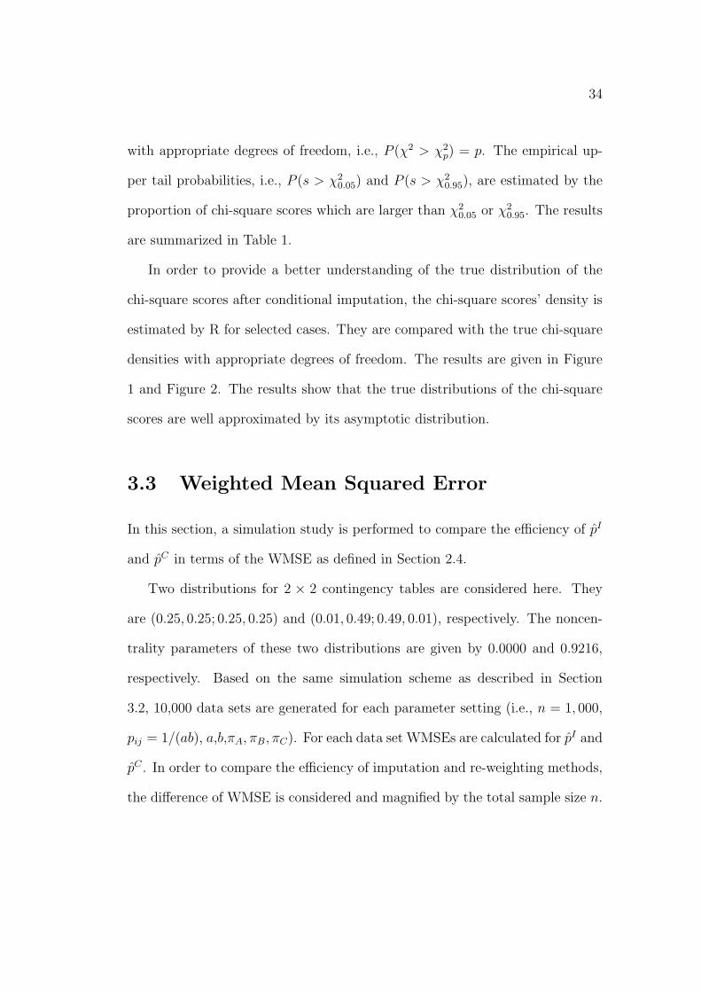
with appropriate degrees of freedom, i.e., P (χ2 > χ2p) = p. The empirical up-

per tail probabilities, i.e., P (s > χ20.05) and P (s > χ2

0.95), are estimated by the

proportion of chi-square scores which are larger than χ20.05 or χ2

0.95. The results

are summarized in Table 1.

In order to provide a better understanding of the true distribution of the

chi-square scores after conditional imputation, the chi-square scores’ density is

estimated by R for selected cases. They are compared with the true chi-square

densities with appropriate degrees of freedom. The results are given in Figure

1 and Figure 2. The results show that the true distributions of the chi-square

scores are well approximated by its asymptotic distribution.

3.3 Weighted Mean Squared Error

In this section, a simulation study is performed to compare the efficiency of pI

and pC in terms of the WMSE as defined in Section 2.4.

Two distributions for 2 × 2 contingency tables are considered here. They

are (0.25, 0.25; 0.25, 0.25) and (0.01, 0.49; 0.49, 0.01), respectively. The noncen-

trality parameters of these two distributions are given by 0.0000 and 0.9216,

respectively. Based on the same simulation scheme as described in Section

3.2, 10,000 data sets are generated for each parameter setting (i.e., n = 1, 000,

pij = 1/(ab), a,b,πA, πB, πC). For each data set WMSEs are calculated for pI and

pC . In order to compare the efficiency of imputation and re-weighting methods,

the difference of WMSE is considered and magnified by the total sample size n.

35

This difference is estimated by the average of 10,000 data sets and is denoted

by ∆. The results are summarized in Table 2 with negative values indicating

better performance of pI .

It can be seen that when the missing probability is large, conditional impu-

tation can improve the efficiency of point estimators.

3.4 Testing for Goodness-of-Fit

Two methods are proposed in Chapter 2 for testing goodness-of-fit. One is

a Wald type statistic and the other is a Rao type statistic. Under the null

hypothesis of testing goodness-of-fit, the Wald type statistic is essentially the

chi-square score constructed in section (3.2). Therefore, in this section we only

study the Rao type statistic.

Based on the same simulation scheme as described in Section 3.2, 10,000

data sets are generated for each parameter setting. For each data set the Rao

score is calculated and compared with appropriate chi-square quantiles. The

empirical upper tail probabilities are estimated by the proportion of the Rao

scores which are larger than the quantiles. The results are summarized in Table

3.

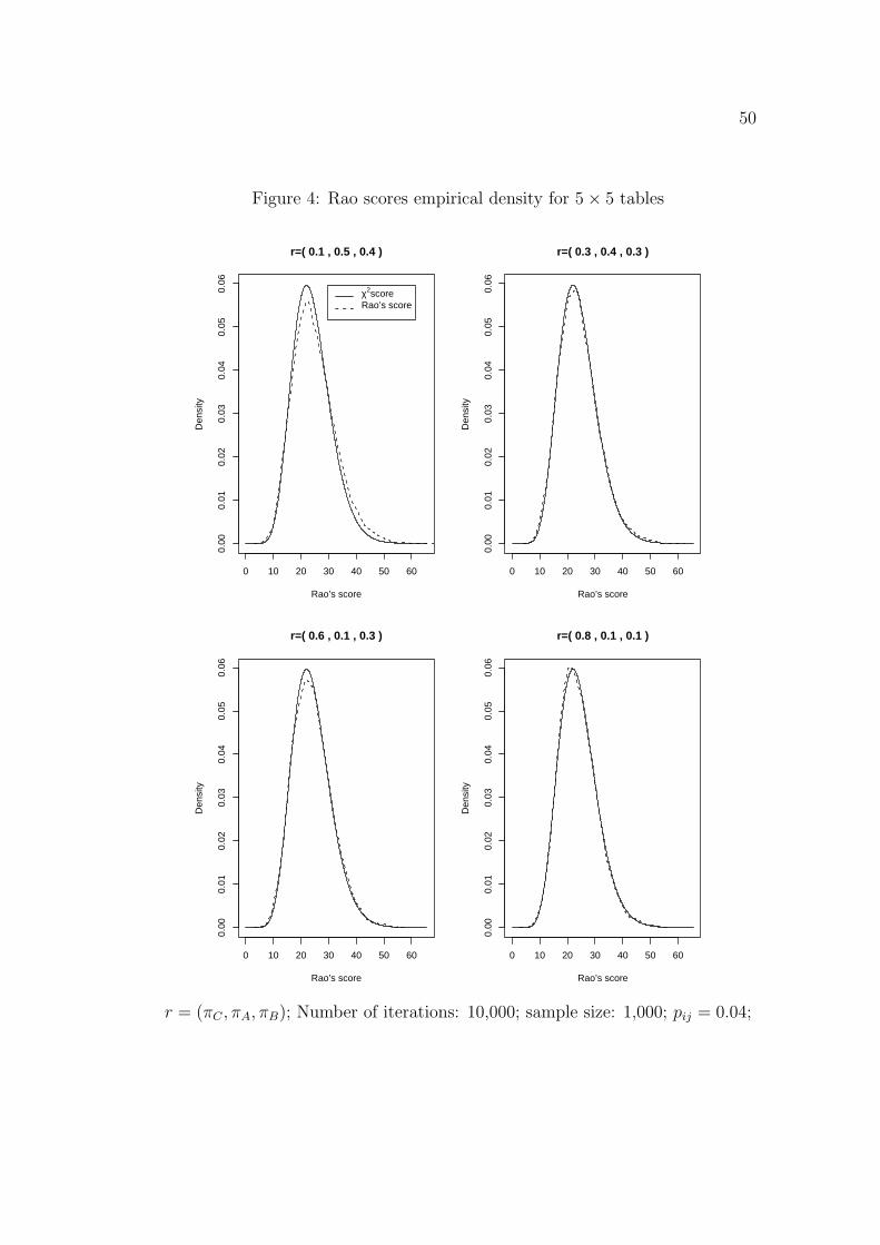
On the other hand, the density of the Rao type statistic is also estimated by

R and compared with the standard one. The results are given in Figure 3 and

4. All the results show that the performance of the Rao type test is comparable

to the Wald type test in terms of type I error.

36

3.5 Testing for Independence

3.5.1 Marginal Imputation

Based on the same simulation scheme described in Section 3.2, 10,000 data sets

are generated for each parameter setting. For each data set marginal imputation

is applied. Then the naive Pearson chi-square score is calculated. According

to our result, the naive Pearson chi-square score should be approximately chi-

square distributed with (a − 1)(b − 1) degrees of freedom. Therefore, it is

compared with the standard chi-square upper quantiles (5% and 95%) with

(a− 1)(b− 1) degrees of freedom. The empirical upper tail probabilities of the

Pearson chi-square scores are estimated. The results are summarized in Table

4.

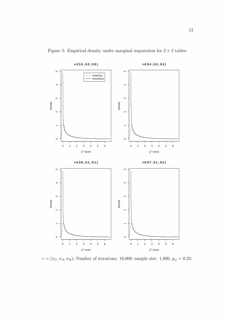
On the other hand, the densities of the naive Pearson scores are also esti-

mated by R and compared with the densities of standard chi-square random

variables with appropriate degrees of freedom. The results are given in Figure

5 and 6.

3.5.2 Conditional Imputation

Based on the same simulation scheme described in Section 3.2, 10,000 data

sets are generated for each parameter setting. For each data set conditional

imputation is applied. The naive Pearson chi-square score is calculated and

corrected by an appropriate constant, which is given in Theorem 4. According to

37

our result, the density of the corrected Pearson scores should be approximately

chi-square distributed with (a − 1)(b − 1) degrees of freedom. Therefore, the

corrected Pearson scores are compared with the standard chi-square quantiles

(5% and 95%) with appropriate degrees of freedom. The empirical upper tail

probabilities are estimated. The results are reported in Table 5.

On the other hand, the density of the corrected Pearson scores is also es-

timated by R and compared with the densities of standard chi-square random

variables with appropriate degrees of freedom. The results are given in Figure

7 and 8.

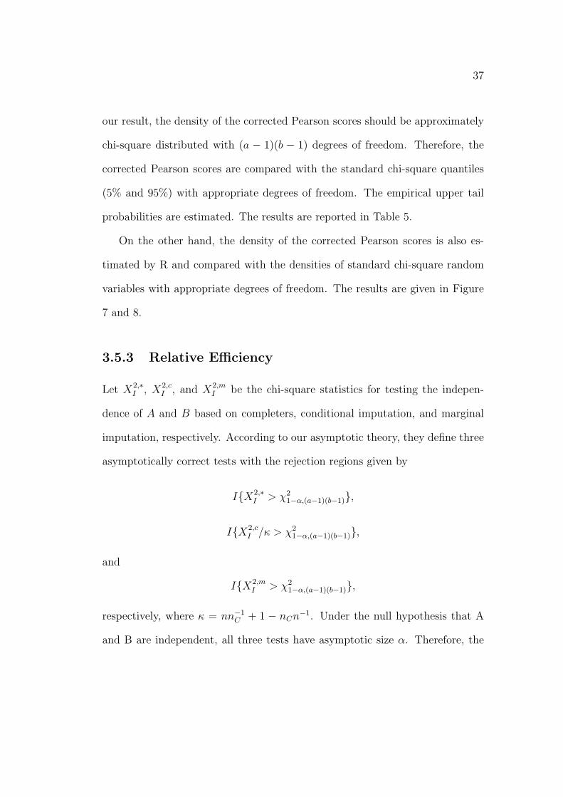
3.5.3 Relative Efficiency

Let X2,∗I , X2,c

I , and X2,mI be the chi-square statistics for testing the indepen-

dence of A and B based on completers, conditional imputation, and marginal

imputation, respectively. According to our asymptotic theory, they define three

asymptotically correct tests with the rejection regions given by

I{X2,∗I > χ2

1−α,(a−1)(b−1)},

I{X2,cI /κ > χ2

1−α,(a−1)(b−1)},

and

I{X2,mI > χ2

1−α,(a−1)(b−1)},

respectively, where κ = nn−1C + 1 − nCn−1. Under the null hypothesis that A

and B are independent, all three tests have asymptotic size α. Therefore, the

38

relative efficiency of the three tests becomes a problem of interest.

In this section, a simulation study is performed to study the relative effi-

ciency of the above three tests in terms of power. The simulation is performed

based on a 2 × 2 contingency table with distribution (0.28,0.22; 0.22,0.28).

Thirty-two different missing patterns are considered. For each parameter set-

ting, 10,000 data sets are generated and three different chi-square scores are

calculated. One is based on the re-weighting method, one is Pearson’s test after

marginal imputation, and the other is the corrected Pearson test after condi-

tional imputation. The power is estimated by the proportion of the scores which

correctly reject the null hypothesis. The results are summarized in Table 6.

In order to have a better understanding of how the power of the three tests

changes as a function of πC , we perform a simulation based on a 2 × 2 contin-

gency table with distribution (0.28, 0.22; 0.22, 0.28). For a given probability of

completeness (πC), we set πA = πB = (1 − πC)/2. Fifty different values of πC ,

which are evenly distributed between 0.1 and 1.0, are studied. For each given

parameter setting, 10,000 iterations are carried out. The estimated empirical

power is plotted versus the πC . The results are given in Figure 9.

We also study the power of the three tests as the function of the non-

centrality parameter δ. In this case, we fix the missing pattern to be

(πC , πA, πB) = (0.5, 0.3, 0.2).

39

Note that the following type of 2× 2 contingency tables

w =

0.25 0.25

0.25 0.25

+

√δ

16

1 −1

−1 1

has non-centrality parameter equal to δ/16, which is proportional to δ. There-

fore, simulations are performed based on this type of 2× 2 contingency tables.

Fifty equally spaced δ values from 0.01 to 0.50 are studied. The estimated

empirical power is plotted versus δ and is given in Figure 10.

The results in this section suggest that when testing independence, greatest

power is achieved by using the complete units only. In contrast, using the

chi-square test under marginal imputation results in the smallest power. An

intuitive explanation is that marginal imputation makes the two categorical

responses of the incompleters independent with each other conditional on the

completers. It decreases the dependency of these two components. The effect

is even more pronounced when the proportion of incompleters is large. As a

result, the power of marginal imputation for testing independence is the lowest.

On the other hand, since the conditional imputation successfully captures the

dependent structure of the two responses, its power is significantly higher than

marginal imputation and comparable to, but not as good as, the re-weighting

method due to the fact that additional noise is created by imputation.

However, the merit of the marginal imputation is that the naive Pearson

test statistic is still valid, which indicates that the marginally imputed data

set can be processed by standard software without modification. This is useful

40

when the proportion of the nonrespondents is not too large. If the proportion

of the incompleters is relatively large, conditional imputation is recommended.

Therefore, the naive Pearson statistic should be modified by a constant which

depends on the proportion of complete units only.

3.6 Conclusion

For the selected sample sizes and parameters, our simulation results show that

the empirical distribution of all the Wald type statistics can be well approxi-

mated by the derived asymptotic distributions.

In addition, the simulation demonstrates that the empirical distributions of

all the Rao type statistics can be well approximated by standard chi-square

distributions with appropriate degrees of freedom.

With regard to testing independence by different methods (re-weighting,

marginal imputation, or conditional imputation) the simulation results indicate

that greatest power is achieved by using the complete units only. In contrast, us-

ing the chi-square test under marginal imputation results in the smallest power.

41

Table 1: Empirical upper tail probability of Wald type statistic

Missing Probability 2× 2 5× 5πC πA πB p0.05 p0.95 p0.05 p0.95

0.1 0.0 0.9 0.042 0.565 0.003 0.2180.1 0.1 0.8 0.042 0.660 0.008 0.3820.1 0.2 0.7 0.044 0.780 0.017 0.6340.1 0.3 0.6 0.047 0.886 0.031 0.8400.1 0.4 0.5 0.049 0.938 0.046 0.9210.2 0.0 0.8 0.046 0.711 0.010 0.4830.2 0.1 0.7 0.047 0.795 0.019 0.6750.2 0.2 0.6 0.046 0.874 0.030 0.8340.2 0.3 0.5 0.049 0.930 0.038 0.9210.2 0.4 0.4 0.048 0.947 0.047 0.9490.3 0.0 0.7 0.046 0.792 0.019 0.6590.3 0.1 0.6 0.050 0.860 0.028 0.8080.3 0.2 0.5 0.050 0.916 0.038 0.9000.3 0.3 0.4 0.053 0.948 0.047 0.9430.3 0.4 0.3 0.052 0.948 0.047 0.9430.4 0.0 0.6 0.047 0.840 0.023 0.7700.4 0.1 0.5 0.048 0.896 0.036 0.8800.4 0.2 0.4 0.056 0.939 0.043 0.9290.4 0.3 0.3 0.048 0.946 0.051 0.9480.5 0.0 0.5 0.049 0.878 0.033 0.8500.5 0.1 0.4 0.046 0.920 0.039 0.9140.5 0.2 0.3 0.045 0.948 0.045 0.9460.6 0.0 0.4 0.055 0.902 0.036 0.8890.6 0.1 0.3 0.045 0.938 0.045 0.9360.6 0.2 0.2 0.052 0.955 0.050 0.9460.7 0.0 0.3 0.048 0.922 0.042 0.9200.7 0.1 0.2 0.051 0.950 0.050 0.9470.7 0.2 0.1 0.049 0.948 0.049 0.9480.8 0.0 0.2 0.050 0.938 0.045 0.9380.8 0.1 0.1 0.052 0.946 0.052 0.9480.9 0.0 0.1 0.051 0.952 0.048 0.9521.0 0.0 0.0 0.053 0.949 0.046 0.950

Number of iterations: 10,000; sample size: 1,000; pij = 1/(ab);p0.05 and p0.95: 5% and 95% empirical upper tail probabilities, respectively.

42

Table 2: Efficiency comparison by WMSE

Missing Probability δ = 0.0000 δ = 0.9216

pC pA pB ∆ ∆0.1 0.0 0.9 −7.13 −7.090.1 0.1 0.8 −8.69 −8.940.1 0.2 0.7 −9.93 −10.170.1 0.3 0.6 −10.64 −10.740.1 0.4 0.5 −11.24 −11.240.2 0.0 0.8 −2.51 −2.490.2 0.1 0.7 −3.13 −3.010.2 0.2 0.6 −3.48 −3.700.2 0.3 0.5 −3.77 −3.800.2 0.4 0.4 −4.10 −4.120.3 0.0 0.7 −0.84 −0.940.3 0.1 0.6 −1.30 −1.350.3 0.2 0.5 −1.57 −1.580.3 0.3 0.4 −1.79 −1.780.3 0.4 0.3 −1.73 −1.750.4 0.0 0.6 −0.25 −0.270.4 0.1 0.5 −0.52 −0.520.4 0.2 0.4 −0.71 −0.690.4 0.3 0.3 −0.69 −0.700.5 0.0 0.5 0.00 −0.030.5 0.1 0.4 −0.12 −0.140.5 0.2 0.3 −0.24 −0.260.6 0.0 0.4 0.19 0.150.6 0.1 0.3 0.03 −0.010.6 0.2 0.2 −0.05 0.030.7 0.0 0.3 0.15 0.180.7 0.1 0.2 0.10 0.100.7 0.2 0.1 0.16 0.090.8 0.0 0.2 0.14 0.160.8 0.1 0.1 0.12 0.130.9 0.0 0.1 0.10 0.081.0 0.0 0.0 0.00 0.00

Number of iterations: 10,000; sample size: 1,000; p0.05 and p0.95: 5% and 95%empirical upper tail probabilities, respectively; δ=0 comes from distribution

p = (0.25, 0.25; 0.25, 0.25) and δ=0.9216 comes from distributionp = (0.01, 0.49; 0.49, 0.01).

43

Table 3: Empirical upper tail probability of Rao type statistic

Missing Probability 2× 2 5× 5πC πA πB p0.05 p0.95 p0.05 p0.95

0.1 0.0 0.9 0.083 0.928 0.054 0.9100.1 0.1 0.8 0.068 0.930 0.054 0.9180.1 0.2 0.7 0.065 0.932 0.052 0.9220.1 0.3 0.6 0.064 0.935 0.058 0.9220.1 0.4 0.5 0.059 0.934 0.055 0.9230.2 0.0 0.8 0.068 0.935 0.057 0.9300.2 0.1 0.7 0.066 0.937 0.056 0.9320.2 0.2 0.6 0.060 0.939 0.054 0.9400.2 0.3 0.5 0.054 0.941 0.054 0.9360.2 0.4 0.4 0.052 0.938 0.059 0.9360.3 0.0 0.7 0.061 0.938 0.054 0.9380.3 0.1 0.6 0.058 0.937 0.054 0.9410.3 0.2 0.5 0.055 0.946 0.055 0.9430.3 0.3 0.4 0.050 0.947 0.053 0.9400.3 0.4 0.3 0.053 0.947 0.050 0.9440.4 0.0 0.6 0.056 0.943 0.052 0.9430.4 0.1 0.5 0.054 0.946 0.051 0.9460.4 0.2 0.4 0.052 0.943 0.056 0.9460.4 0.3 0.3 0.055 0.950 0.051 0.9460.5 0.0 0.5 0.053 0.937 0.052 0.9480.5 0.1 0.4 0.053 0.942 0.051 0.9460.5 0.2 0.3 0.051 0.948 0.053 0.9480.6 0.0 0.4 0.054 0.944 0.055 0.9440.6 0.1 0.3 0.049 0.948 0.050 0.9490.6 0.2 0.2 0.051 0.951 0.051 0.9440.7 0.0 0.3 0.050 0.950 0.052 0.9480.7 0.1 0.2 0.052 0.947 0.052 0.9460.7 0.2 0.1 0.047 0.951 0.051 0.9490.8 0.0 0.2 0.050 0.949 0.051 0.9510.8 0.1 0.1 0.049 0.950 0.050 0.9440.9 0.0 0.1 0.051 0.946 0.050 0.9471.0 0.0 0.0 0.052 0.949 0.046 0.950

Number of iterations: 10,000; sample size: 1,000; pij = 1/(ab);p0.05 and p0.95: 5% and 95% empirical upper tail probabilities, respectively.

44

Table 4: Testing independence under marginal imputation

Missing Probability 2× 2 5× 5πC πA πB p0.05 p0.95 p0.05 p0.95

0.1 0.0 0.9 0.051 0.952 0.048 0.9480.1 0.1 0.8 0.051 0.950 0.051 0.9500.1 0.2 0.7 0.049 0.952 0.050 0.9500.1 0.3 0.6 0.048 0.952 0.052 0.9500.1 0.4 0.5 0.050 0.950 0.047 0.9500.2 0.0 0.8 0.048 0.951 0.048 0.9510.2 0.1 0.7 0.050 0.948 0.046 0.9480.2 0.2 0.6 0.050 0.950 0.048 0.9510.2 0.3 0.5 0.051 0.947 0.050 0.9500.2 0.4 0.4 0.052 0.951 0.051 0.9490.3 0.0 0.7 0.049 0.949 0.047 0.9490.3 0.1 0.6 0.050 0.948 0.050 0.9470.3 0.2 0.5 0.047 0.953 0.049 0.9470.3 0.3 0.4 0.049 0.954 0.048 0.9490.3 0.4 0.3 0.048 0.948 0.045 0.9540.4 0.0 0.6 0.049 0.949 0.051 0.9510.4 0.1 0.5 0.045 0.953 0.051 0.9490.4 0.2 0.4 0.049 0.950 0.050 0.9500.4 0.3 0.3 0.047 0.949 0.045 0.9480.5 0.0 0.5 0.050 0.952 0.048 0.9500.5 0.1 0.4 0.046 0.956 0.049 0.9480.5 0.2 0.3 0.049 0.952 0.052 0.9470.6 0.0 0.4 0.046 0.949 0.048 0.9520.6 0.1 0.3 0.049 0.948 0.046 0.9490.6 0.2 0.2 0.051 0.947 0.049 0.9520.7 0.0 0.3 0.052 0.946 0.049 0.9470.7 0.1 0.2 0.049 0.948 0.046 0.9540.7 0.2 0.1 0.048 0.954 0.052 0.9520.8 0.0 0.2 0.049 0.952 0.051 0.9500.8 0.1 0.1 0.050 0.949 0.047 0.9450.9 0.0 0.1 0.051 0.949 0.048 0.9481.0 0.0 0.0 0.047 0.950 0.052 0.956

Number of iterations: 10,000; sample size: 1,000; pij = 1/(ab);p0.05 and p0.95: 5% and 95% empirical upper tail probabilities, respectively.

45

Table 5: Testing independence under conditional imputation

Missing Probability 2× 2 5× 5πC πA πB p0.05 p0.95 p0.05 p0.95

0.1 0.0 0.9 0.054 0.944 0.040 0.9280.1 0.1 0.8 0.049 0.950 0.038 0.9320.1 0.2 0.7 0.047 0.946 0.038 0.9330.1 0.3 0.6 0.047 0.947 0.039 0.9280.1 0.4 0.5 0.053 0.946 0.036 0.9300.2 0.0 0.8 0.049 0.951 0.044 0.9440.2 0.1 0.7 0.050 0.948 0.042 0.9410.2 0.2 0.6 0.048 0.949 0.044 0.9450.2 0.3 0.5 0.049 0.949 0.044 0.9420.2 0.4 0.4 0.047 0.943 0.046 0.9430.3 0.0 0.7 0.050 0.947 0.047 0.9450.3 0.1 0.6 0.052 0.945 0.043 0.9490.3 0.2 0.5 0.050 0.952 0.046 0.9470.3 0.3 0.4 0.054 0.951 0.046 0.9480.3 0.4 0.3 0.052 0.949 0.045 0.9500.4 0.0 0.6 0.052 0.947 0.045 0.9480.4 0.1 0.5 0.047 0.947 0.046 0.9510.4 0.2 0.4 0.046 0.950 0.047 0.9480.4 0.3 0.3 0.050 0.951 0.046 0.9490.5 0.0 0.5 0.048 0.948 0.047 0.9500.5 0.1 0.4 0.052 0.946 0.046 0.9510.5 0.2 0.3 0.044 0.950 0.048 0.9510.6 0.0 0.4 0.048 0.951 0.047 0.9500.6 0.1 0.3 0.050 0.950 0.046 0.9520.6 0.2 0.2 0.052 0.950 0.049 0.9460.7 0.0 0.3 0.052 0.949 0.050 0.9510.7 0.1 0.2 0.051 0.946 0.048 0.9510.7 0.2 0.1 0.053 0.951 0.046 0.9500.8 0.0 0.2 0.052 0.953 0.046 0.9470.8 0.1 0.1 0.052 0.949 0.052 0.9480.9 0.0 0.1 0.054 0.948 0.049 0.9501.0 0.0 0.0 0.045 0.948 0.047 0.950

Number of iterations: 10,000; sample size: 1,000; pij = 1/(ab);p0.05 and p0.95: 5% and 95% empirical upper tail probabilities, respectively.

46

Table 6: Power comparison for testing independence

Missing Probability δ = 0.0000 δ = 0.0144

πC πA πB X2,∗I X2,m

I X2,cI X2,∗

I X2,mI X2,c

I

0.1 0.0 0.9 0.055 0.050 0.053 0.219 0.069 0.2070.1 0.1 0.8 0.049 0.050 0.055 0.224 0.064 0.2080.1 0.2 0.7 0.053 0.050 0.053 0.227 0.065 0.2180.1 0.3 0.6 0.050 0.046 0.052 0.221 0.070 0.2130.1 0.4 0.5 0.054 0.050 0.056 0.228 0.071 0.2110.2 0.0 0.8 0.048 0.048 0.049 0.401 0.116 0.3510.2 0.1 0.7 0.049 0.050 0.050 0.390 0.116 0.3450.2 0.2 0.6 0.050 0.054 0.052 0.398 0.114 0.3570.2 0.3 0.5 0.052 0.050 0.050 0.403 0.124 0.3560.2 0.4 0.4 0.053 0.054 0.052 0.398 0.117 0.3580.3 0.0 0.7 0.050 0.051 0.048 0.552 0.210 0.4810.3 0.1 0.6 0.048 0.054 0.049 0.546 0.205 0.4680.3 0.2 0.5 0.046 0.050 0.048 0.542 0.202 0.4760.3 0.3 0.4 0.050 0.055 0.049 0.544 0.202 0.4700.3 0.4 0.3 0.049 0.051 0.048 0.561 0.208 0.4850.4 0.0 0.6 0.047 0.050 0.048 0.672 0.330 0.5810.4 0.1 0.5 0.049 0.050 0.052 0.670 0.328 0.5730.4 0.2 0.4 0.050 0.047 0.052 0.664 0.328 0.5800.4 0.3 0.3 0.050 0.053 0.048 0.667 0.321 0.5780.5 0.0 0.5 0.048 0.052 0.048 0.763 0.478 0.6700.5 0.1 0.4 0.052 0.050 0.053 0.766 0.476 0.6750.5 0.2 0.3 0.050 0.056 0.049 0.763 0.475 0.6700.6 0.0 0.4 0.049 0.048 0.052 0.837 0.632 0.7540.6 0.1 0.3 0.047 0.050 0.049 0.837 0.620 0.7510.6 0.2 0.2 0.051 0.052 0.051 0.834 0.623 0.7520.7 0.0 0.3 0.052 0.051 0.054 0.889 0.758 0.8230.7 0.1 0.2 0.053 0.050 0.049 0.893 0.760 0.8270.7 0.2 0.1 0.047 0.048 0.048 0.883 0.757 0.8240.8 0.0 0.2 0.055 0.052 0.053 0.920 0.859 0.8820.8 0.1 0.1 0.051 0.049 0.051 0.922 0.861 0.8880.9 0.0 0.1 0.048 0.047 0.048 0.948 0.925 0.9331.0 0.0 0.0 0.046 0.046 0.046 0.963 0.963 0.963

Number of iterations: 10,000; sample size: 1,000; pij = (0.28, 0.22; 0.22, 0.28);p0.05 and p0.95: 5% and 95% empirical upper tail probabilities, respectively.

47

Figure 1: Wald’s empirical density for 2× 2 tables

0 5 10 15 20

0.00

0.05

0.10

0.15

0.20

0.25

r=( 0.1 , 0.5 , 0.4 )

χ2−score

Den

sity

theoreticalempirical

0 5 10 15 20

0.00

0.05

0.10

0.15

0.20

0.25

r=( 0.8 , 0.1 , 0.1 )

χ2−score

Den

sity

0 5 10 15 20

0.00

0.05

0.10

0.15

0.20

0.25

r=( 0.2 , 0.3 , 0.5 )

χ2−score

Den

sity

0 5 10 15 20

0.00

0.05

0.10

0.15

0.20

0.25

r=( 0.2 , 0.4 , 0.4 )

χ2−score

Den

sity

r = (πC , πA, πB); Number of iterations: 10,000; sample size: 1,000; pij = 0.25;

48

Figure 2: Wald’s empirical density for 5× 5 tables

0 10 20 30 40 50 60

0.00

0.01

0.02

0.03

0.04

0.05

0.06

r=( 0.1 , 0.5 , 0.4 )

χ2−score

Den

sity

theoreticalempirical

0 10 20 30 40 50 60

0.00

0.01

0.02

0.03

0.04

0.05

0.06

r=( 0.8 , 0.1 , 0.1 )

χ2−score

Den

sity

0 10 20 30 40 50 60

0.00

0.01

0.02

0.03

0.04

0.05

0.06

r=( 0.2 , 0.3 , 0.5 )

χ2−score

Den

sity

0 10 20 30 40 50 60

0.00

0.01

0.02

0.03

0.04

0.05

0.06

r=( 0.2 , 0.4 , 0.4 )

χ2−score

Den

sity

r = (πC , πA, πB); Number of iterations: 10,000; sample size: 1,000; pij = 0.04;

49

Figure 3: Rao scores empirical density for 2× 2 tables

0 5 10 15 20 25

0.00

0.05

0.10

0.15

0.20

0.25

r=( 0.1 , 0.5 , 0.4 )

Rao’s score

Den

sity

χ2scoreRao’s score

0 5 10 15 20 25

0.00

0.05

0.10

0.15

0.20

0.25

r=( 0.3 , 0.4 , 0.3 )

Rao’s score

Den

sity

0 5 10 15 20 25

0.00

0.05

0.10

0.15

0.20

0.25

r=( 0.6 , 0.1 , 0.3 )

Rao’s score

Den

sity

0 5 10 15 20 25

0.00

0.05

0.10

0.15

0.20

0.25

r=( 0.8 , 0.1 , 0.1 )

Rao’s score

Den

sity

r = (πC , πA, πB); Number of iterations: 10,000; sample size: 1,000; pij = 0.25;

50

Figure 4: Rao scores empirical density for 5× 5 tables

0 10 20 30 40 50 60

0.00

0.01

0.02

0.03

0.04

0.05

0.06

r=( 0.1 , 0.5 , 0.4 )

Rao’s score

Den

sity

χ2scoreRao’s score

0 10 20 30 40 50 60

0.00

0.01

0.02

0.03

0.04

0.05

0.06

r=( 0.3 , 0.4 , 0.3 )

Rao’s score

Den

sity

0 10 20 30 40 50 60

0.00

0.01

0.02

0.03

0.04

0.05

0.06

r=( 0.6 , 0.1 , 0.3 )

Rao’s score

Den

sity

0 10 20 30 40 50 60

0.00

0.01

0.02

0.03

0.04

0.05

0.06

r=( 0.8 , 0.1 , 0.1 )

Rao’s score

Den

sity

r = (πC , πA, πB); Number of iterations: 10,000; sample size: 1,000; pij = 0.04;

51

Figure 5: Empirical density under marginal imputation for 2× 2 tables

0 1 2 3 4 5 6

01

23

45

r=( 0.3 , 0.3 , 0.5 )

χ2−score

Den

sity

empiricaltheoretical

0 1 2 3 4 5 6

01

23

45

r=( 0.4 , 0.3 , 0.3 )

χ2−score

Den

sity

0 1 2 3 4 5 6

01

23

45

r=( 0.8 , 0.1 , 0.1 )

χ2−score

Den

sity

0 1 2 3 4 5 6

01

23

45

r=( 0.7 , 0.1 , 0.2 )

χ2−score

Den

sity

r = (πC , πA, πB); Number of iterations: 10,000; sample size: 1,000; pij = 0.25;

52

Figure 6: Empirical density under marginal imputation for 5× 5 tables

0 5 10 15 20 25 30

0.00

0.02

0.04

0.06

r=( 0.3 , 0.3 , 0.5 )

χ2−score

Den

sity

empiricaltheoretical

0 5 10 15 20 25 30

0.00

0.02

0.04

0.06

r=( 0.4 , 0.3 , 0.3 )

χ2−score

Den

sity

0 5 10 15 20 25 30

0.00

0.02

0.04

0.06

r=( 0.8 , 0.1 , 0.1 )

χ2−score

Den

sity

0 5 10 15 20 25 30

0.00

0.02

0.04

0.06

r=( 0.7 , 0.1 , 0.2 )

χ2−score

Den

sity

r = (πC , πA, πB); Number of iterations: 10,000; sample size: 1,000; pij = 0.04;

53

Figure 7: Empirical density under conditional imputation for 2× 2 tables

0 1 2 3 4 5 6

01

23

45

r=( 0.3 , 0.3 , 0.5 )

χ2−score

Den

sity

empiricaltheoretical

0 1 2 3 4 5 6

01

23

45

r=( 0.4 , 0.3 , 0.3 )

χ2−score

Den

sity

0 1 2 3 4 5 6

01

23

45

r=( 0.8 , 0.1 , 0.1 )

χ2−score

Den

sity

0 1 2 3 4 5 6

01

23

45

r=( 0.7 , 0.1 , 0.2 )

χ2−score

Den

sity

r = (πC , πA, πB); Number of iterations: 10,000; sample size: 1,000; pij = 0.25;

54

Figure 8: Empirical density under conditional imputation for 5× 5 tables

0 5 10 15 20 25 30

0.00

0.02

0.04

0.06

r=( 0.3 , 0.3 , 0.5 )

χ2−score

Den

sity

empiricaltheoretical

0 5 10 15 20 25 30

0.00

0.02

0.04

0.06

r=( 0.4 , 0.3 , 0.3 )

χ2−score

Den

sity

0 5 10 15 20 25 30

0.00

0.02

0.04

0.06

r=( 0.8 , 0.1 , 0.1 )

χ2−score

Den

sity

0 5 10 15 20 25 30

0.00

0.02

0.04

0.06

r=( 0.7 , 0.1 , 0.2 )

χ2−score

Den

sity

r = (πC , πA, πB); Number of iterations: 10,000; sample size: 1,000; pij = 0.04;

55

Figure 9: Power of testing independence vs. πC .

0.2 0.4 0.6 0.8 1.0

0.2

0.4

0.6

0.8

1.0

πC

Pow

er

Re−Weighting MethodMarginal ImputationConditonal Imputation

πA = πB = (1− πC)/2; Number of iterations: 10,000; sample size: 1,000;p = (0.28, 0.22; 0.22, 0.28);

56

Figure 10: Power of testing independence vs. δ.

0.0 0.1 0.2 0.3 0.4 0.5

0.2

0.4

0.6

0.8

1.0

δ

Pow

er

Re−Weighting MethodMarginal ImputationConditonal Imputation

(πC , πA, πB) = (0.5, 0.3, 0.2); Number of iterations: 10,000; sample size: 1,000;

p = (0.25, 0.25; 0.25, 0.25) +√

δ16

(1,−1;−1, 1);

57

Chapter 4

Imputation Under Stratified

Sampling

4.1 Introduction

In the previous chapters, we have studied various imputation methods under

simple random sampling. In sample survey problems, however, stratified sam-

pling is more frequently considered. Therefore, in this chapter, we study statis-

tical properties of conditional imputation under stratified sampling.

For stratified sampling, an additional index for stratum is added to various

quantities. For example, for simple random sampling, nC is the number of

completers, but for stratified sampling, nCh denotes the number of completers

within the hth stratum. Quantities nAh , nB

h , ph, ph,ij, ph,i·, and ph,·j are similarly

defined. Within the hth stratum, we assume that a simple random sample of

size nh = nAh + nB

h + nCh is obtained, and samples across strata are obtained

independently. The total sample size is given by n =∑H

h=1 nh, where H is the

number of strata. The overall probability distribution vector is p =∑H

h=1 whph

and its estimator is pI =∑

whpIh, where wh is the known stratum weight.

58

In practice, one usually encounters one of the following two situations

1. H is fixed and nh/n → ρh > 0, h = 1, ..., H.

2. H is large and {nh : h = 1, 2, ...} is bounded.

For the first situation, two types of conditional imputation methods are studied.

One is the method of imputation within stratum and the other is the method

of imputation across strata. For the second situation, since nh is small, we

may observe some strata without any completer. Therefore, the method of

imputation within stratum may not be applicable to this situation. Instead, the

method of imputation across strata is applied. For different imputation methods

under different situations, the asymptotic distributions of point estimators are

derived and appropriate tests are studied.

The rest of this chapter is arranged as following. In Section 4.2, the method

of imputation within stratum is studied under situation 1. In Sections 4.3 and

4.4, the method of imputation across strata is studied under situation 1 and

situation 2, respectively.

4.2 Imputation Within Each Stratum

4.2.1 Asymptotic Distribution

We first consider the simple case where H is fixed and nh is large. In this

case, strata are often used as imputation classes. Even if strata are not used

59

as imputation classes (i.e., each imputation class may contain several strata),

imputation within each stratum is often applied when nh is large.

A direct generalization of Theorem 2 leads to the following theorem.

Theorem 5 Assume that conditional imputation is carried out within each stra-

tum under the situation 1. Then

√n(pI − p) →d N(0, Σ∗),

as n →∞ and

Σ∗ =H∑

h=1

w2h

ρh

Σh, (4.1)

where Σh is the Σ in Theorem 2 but within the hth stratum.

Proof:

It can be noted that

√n(pI − p) =

√n

∑wh(p

Ih − ph)

=∑

wh

√n

nh

√nh(p

Ih − ph)

=∑ wh√

ρh

√nh(p

Ih − ph) + op(1).

According to Theorem 2,

√nh(p

Ih − ph) → N(0, Σh),

60

where Σh is the asymptotic covariance matrix of√

nh(ph − p) which can be

calculated according to Theorem 2.

Therefore,

√n(pI − p) →d

∑

h

wh√ρh

N(0, Σh) = N(0,∑

h

w2h

ρh

Σh).

Based on (4.1), a Wald type test can be constructed for a general hypothesis

H0 : R(p) = 0 vs. HA : R(p) 6= 0,

where R is a first order differentiable function from Ra×b to Rd for some d. Let

C(p) =∂R(p)

∂p.

Assume C(p) has full rank. It follows that

√n[R(pI)−R(p)] = C(p)

√n(pI − p) + op(1)

→d N(0, C(p)Σ∗[C(p)]′),

where Σ∗ is given in (4.1). Therefore, a Wald type statistic can be obtained by

W = n[R(pI)−R(p)]′[C(p)Σ∗C ′(p)]−1[R(pI)−R(p)],

which under the null hypothesis is asymptotically distributed as a χ2 random

variable with d degrees of freedom.

61

4.2.2 Rao’s Test for Goodness-of-Fit

Although the Wald type test is asymptotically valid, it is difficult to implement

due to the complexity of the covariance matrix. Therefore, the Rao type test,

which is proposed in Section 2.5, is studied.

The naive Pearson statistic is given by

X2P = n

∑ (pIij − pij)

2

pij

.

Since the asymptotic covariance of pI is given by Σ∗, the first order moment of

X2P can be approximated by

λ = λ(πh,A, πh,B, πh,C , ph) = tr(diag{1/√p}Σ∗diag{1/√p}), (4.2)

where

1/√

p = (1/√

p11, · · · , 1/√

p1b, · · · , 1/√

pa1, · · · , 1/√

pab)′.

However, unlike the situation for simple random sampling, a closed formula

for λ does not exist due to the complexity of Σ∗. Instead, we propose the

following bootstrap procedure to estimate λ.

Let Sh denote the data set from the hth stratum. Our proposed bootstrap

procedure is outlined below:

(1) Perform conditional imputation within each Sh;

(2) Get estimators πh,A, πh,B, πh,C , and pIh;

(3) Generate the bootstrap data set S∗h by treating πh,A, πh,B, πh,C , and pIh as

the true probabilities;

62

(4) Perform conditional imputation for each S∗h;

(5) Get the overall probability estimator (pI∗) based on the imputed bootstrap

data set;

(6) Calculated the naive Pearson statistic based on the bootstrap data set,

i.e.,

X2∗P = n

∑ (pI∗ij − pI

ij)2

pIij

.

(7) Repeat steps (3)-(6) B times and average the B naive Pearson statistics

(X2∗P ), which gives λ (an estimator for λ);

(8) Finally, the Rao statistic is given by

ab− 1

λn

∑ij

(pIij − pij)

2

pij

.

It can be seen that, conditional on Sh, h = 1, · · · , H, each S∗h has the same

type of distribution as Sh but with different parameters. In other words, the

distribution of Sh is determined by {πh,A, πh,B, πh,C , ph}, while the distribution

of S∗h is determined by {πh,A, πh,B, πh,C , pIh}. Therefore, conditional on Sh, λ

provides a consistent estimator for λ(πh,A, πh,B, πh,C , pIh). On the other hand,

λ is a continuous function of {πh,A, πh,B, πh,C , ph}, and (πh,A, πh,B, πh,C) →a.s

(πh,A, πh,B, πh,C), pIh →a.s ph. Therefore, λ is a consistent estimator of λ.

4.3 Imputation Across Strata with Small H

In this section, we study the method of imputation across strata with small H.

63

For a sampled incomplete unit, e.g., (A,B) = (i, ∗), the missing value is

imputed by j according to the conditional probability

pij|A.= P (B = j|A = i and B is missing)

=P ((A,B) = (i, j) and B is missing)

P (A = i and B is missing)

=

∑h P ((A, B) from strata h,A = i, B = j, and B is missing)∑

h P ((A,B) from strata h,A = i and B is missing)

=

∑h whπh,Aph,ij∑h whπh,Aph,i·

.

Note that in this situation since we have a large sample size for each stratum,

we do not need to assume (πh,A, πh,B, πh,C) are the same for different stratum.

Similarly, for a sampled unit with (A,B) = (∗, j), the missing value is imputed

by i according to the conditional probability

pij|B.=

∑whπh,Bph,ij∑whπh,Bph,·j

.

To carry out imputation, the parameters πh,A, πh,B, ph,ij, ph,i·, and ph,·j should

be replaced by their estimators, e.g., nAh /nh for πh,A and nC

h,ij/nCh for ph,ij.

4.3.1 Asymptotic Distribution

Theorem 6 Assume that H is fixed and nh/n → ρh > 0, h = 1, ..., H. Based

on conditional imputation across strata, we have that

√n(pI − p) →d N(0, Σ1 + Σ2),

64

where

Σ1 =∑

h

w2h

ρh

MhPhM′h

Σ2 =∑

h

[w2

h

ρh

(πh,AΣAh + πh,BΣB

h )

]

Mh =1√πh,C

I − πh,A√πh,C

NAh (Ia ⊗ Ub)− πh,B√

πh,C

NBh (Ua ⊗ Ib)

Ph = diag(ph)− php′h

NAh = diag(p11|A, · · · , p1b|A, · · · , pa1|A, · · · , pab|A)

NBh = diag(p11|B, · · · , p1b|B, · · · , pa1|B, · · · , pab|B)

ΣAh = diag(ah)− aha

′h

ΣBh = diag(bh)− bhb

′h

ah = (ph,1.p11|A, · · · , ph,1.p1b|A, · · · , ph,a·pa1|A, · · · , ph,a·pab|A)′

bh = (p11|Bph,.1, · · · , p1b|Bph,·b · · · , pa1|Bph,.1, · · · , pab|Bph,·b)′.

Proof:

The overall cell probability estimator after conditional imputation across strata

can be obtained by

pI =∑

whnA

h pAh + nB

h pBh + nC

h pCh

nh

.

Let σ(C) denote the σ-field generated by all completers and {nAh , nB

h , nCh }.

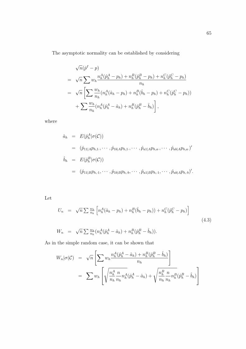
65

The asymptotic normality can be established by considering

√n(pI − p)

=√

n∑

whnA

h (pAh − ph) + nB

h (pBh − ph) + nC

h (pCh − ph)

nh

=√

n

[∑ wh

nh

(nAh (ah − ph) + nB

h (bh − ph) + nCh (pC

h − ph))

+∑ wh

nh

(nAh (pA

h − ah) + nBh (pB

h − bh)

],

where

ah = E(pAh |σ(C))

= (p11|Aph,1·, · · · , p1b|Aph,1·, · · · , pa1|Aph,a·, · · · , pab|Aph,a·)′

bh = E(pBh |σ(C))

= (p11|Bph,·1, · · · , p1b|Bph,·b, · · · , pa1|Bph,·1, · · · , pab|Aph,·b)′.

Let

Un =√

n∑ wh

nh

[nA

h (ah − ph) + nBh (bh − ph)) + nC

h (pCh − ph)

]

Wn =√

n∑ wh

nh(nA

h (pAh − ah) + nB

h (pBh − bh)).

(4.3)

As in the simple random case, it can be shown that

Wn|σ(C) =√

n

[∑wh

nAh (pA

h − ah) + nBh (pB

h − bh)

nh

]

=∑

wh

√nA

h

nh

n

nh

nAh (pA

h − ah) +

√nB

h

nh

n

nh

nBh (pB

h − bh)

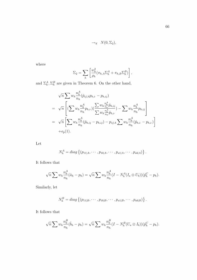
66

→d N(0, Σ2),

where

Σ2 =∑

h

[w2

h

ρh

(πh,AΣAh + πh,BΣB

h )

],

and ΣAh , ΣB

h are given in Theorem 6. On the other hand,

√n

∑wh

nAh

nh

(pij|Aph,i· − ph,ij)

=√

n

(

∑wh

nAh

nh

ph,i·)(

∑wh

nAh

nhph,ij

∑wh

nAh

nhph,i·

)−∑

whnA

h

nh

ph,ij

=√

n

[∑wh

nAh

nh

(ph,ij − ph,ij)− pij|A∑

whnA

h

nh

(ph,i· − ph,i·)]

+op(1).

Let

NAh = diag

{(p11|A, · · · , p1b|A, · · · , pa1|A, · · · , pab|A)

}.

It follows that

√n

∑wh

nAh

nh

(ah − ph) =√

n∑

whnA

h

nh

(I −NAh (Ia ⊗ Ub))(p

Ch − ph).

Similarly, let

NBh = diag

{(p11|B, · · · , p1b|B, · · · , pa1|B, · · · , pab|B)

}.

It follows that

√n

∑wh

nBh

nh

(bh − ph) =√

n∑

whnB

h

nh

(I −NBh (Ua ⊗ Ib))(p

Ch − ph).

67

Consequently,

Un

=√

n

[∑wh(I − nA

h

nh

NAh Ia ⊗ Ub − nB

h

nh

NBh Ua ⊗ Ib)(ph − ph)

]+ op(1)

=∑ wh

√n√

nCh

[I − nA

h

nh

NAh Ia ⊗ Ub − nB

h

nh

NBh Ua ⊗ Ib

]

√nC

h (pCh − ph) + op(1)

=∑ wh√

ρhπh,C

[1− πh,ANA

h (Ia ⊗ Ub)− πh,BNBh (Ua ⊗ Ib)

]

×√

nCh (pC

h − ph) + op(1)

→ N(0, Σ1),

where

Σ1 =∑

h

w2h

ρh

MhPhM′h

Mh =1√πh,C

− πh,A√πh,C

NAh (Ua ⊗ Ib)− πh,B√

πh,C

NBh (Ia ⊗ Ub)

Ph = diag{ph} − php′h.

As a result,

√n(pI − p) = Wn + Un → N(0, Σ1 + Σ2).

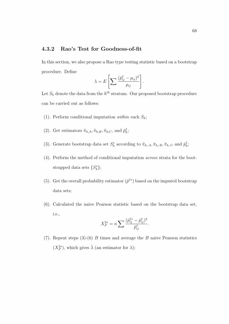
68

4.3.2 Rao’s Test for Goodness-of-fit

In this section, we also propose a Rao type testing statistic based on a bootstrap

procedure. Define

λ = E

[∑ (pIij − pij)

2

pij

].

Let Sh denote the data from the hth stratum. Our proposed bootstrap procedure

can be carried out as follows:

(1). Perform conditional imputation within each Sh;

(2). Get estimators πh,A, πh,B, πh,C , and pIh;

(3). Generate bootstrap data set S∗h according to πh,·A, πh,·B, πh,·C and pIh;

(4). Perform the method of conditional imputation across strata for the boot-

strapped data sets {S∗h};

(5). Get the overall probability estimator (pI∗) based on the imputed bootstrap

data sets;

(6). Calculated the naive Pearson statistic based on the bootstrap data set,

i.e.,

X2∗P = n

∑ (pI∗ij − pI

ij)2

pIij

.

(7). Repeat steps (3)-(6) B times and average the B naive Pearson statistics

(X2∗P ), which gives λ (an estimator for λ);

69

(8). Finally, the Rao statistic is given by

ab− 1

λn

∑ij

(pIij − pij)

2

pij

.

As in the case for imputation within stratum, λ is a continuous function in

(πh,A, πh,B, πh,C , ph). Therefore, λ is a consistent estimator for λ.

4.4 Imputation Across Strata with Large H

In this section, we study the method of imputation across strata with large H.

The entire discussion is based on the Assumption B, given below.

Assumption B:

(1) For all h and some (πA, πB, πC), (πh,A, πh,B, πh,B) = (πA, πB, πC);

(2) 2 ≤ nh ≤ m, ∀h and for some m;

(3) ε1 ≤ Hwh ≤ ε2, ∀h and ∀H;

(4) For all h and i ∈ {1, · · · , a}, j ∈ {1, · · · , b}, δ1 ≤ ph,ij ≤ δ2.

Consequently, pij|A and pij|B, which are defined in Section 4.3, can be simplified

to

pij|A =

∑whph,ij∑whph,i·

and pij|B =

∑whph,ij∑whph,·j

.

Their estimators can be obtained by

pij|A =

∑wh

nCh,ij

nh∑wh

nCh,i·nh

and pij|B =

∑wh

nCh,ij

nh∑wh

nCh,·jnh

.

70

The method of conditional imputation across strata will be based on pij|A and

pij|B. Here Un and Wn are the same as defined in (4.3). In this section, we use

σ(C) to denote all the observed responses, which includes not only all completers

and {nAh , nB

h , nCh }, but also the observed respondents from the incompleters.

4.4.1 Asymptotic Distribution

Lemma 2 Conditional on σ(C), Wn is asymptotically normally distributed.

Proof:

Since conditional on the observed units,

√n

∑wh

nAh (pA

h − E(pAh |σ(C)))

nh

and√

n∑

whnB

h (pBh − E(pB

h |σ(C)))

nh

are independent, it suffices to show the result for either of them. Without loss

of generality, consider

V =√

n∑

whnA

h (pAh − E(pA

h |σ(C)))

nh

,

and assume πA > 0 (otherwise V = 0). Let l be an arbitrary ab-dimensional

vector with lij be its [(i − 1)b + j]th component. Without loss of generality,

assume

l11 = max{lij} and lab = min{lij}.

Assume l11 > lab, otherwise l′V =a.s 0.

71

In order to establish asymptotic normality for V , it suffices to do it for l′V .

This can be done by checking Liapunouv’s condition. Let

σ2n = var[l′V ]

= var[√

n∑

whnA

h

nh

l′(pAh − E(pA

h |σ(C)))]

= Var

[√

n∑

whnA

h

nh

∑ij

lij pAh,i·

nAh,ij

nAh,i·

].

Thus

σ2n = n

∑

h

w2h(

nAh

nh

)2∑

i

(pA

h,i·nA

h,i·)2var(

∑j

lijnAh,ij))

= n∑

h

w2h(

nAh

nh

)2∑

i

(pA

h,i·nA

h,i·)2nA

h,i·

(∑j

pij|A(lij −∑

j′lij′ pij′|A)2

)

≥ n

H2

∑

h

(Hwh)2 (nA

h )2

n2hn

Ah,i·

∑j

(pAh,i·)

2p11|Ap2ab|A(l11 − lab)

2

≥ 1

mH

∑

h

ε21(

nAh

nh

)2δ21 p11|Apab|A(l11 − lab)

2

= ε21(l11 − lab)

2δ21 p11|B p2

ab|A1

mH

∑ (nAh )2

(nh)2.

Note that

pij|A →a.s. pij|A =

∑whpij∑whpi·

≥∑

whδ1∑whbδ2

=δ1

bδ2

> 0,

and

1

H

∑ (nAh )2

n2h

≥(

1

N

∑ nAh

nh

)2

→a.s π2A > 0.

Therefore, it can be concluded that σ2n = Op(1).

72

On the other hand, ∀δ > 0,

∑

h

E|√nwhnA

h

nh

l′(pAh − E(pA

h |σ(C)))|2+δ

≤∑

h

E|√

n

H(Hwh)l

′(pAh + E(pA

h |σ(C)))|2+δ

≤∑

h

n1+δ/2

H2+δε2+δ2 E|l′(pA

h + E(pAh |σ(C)))|2+δ

≤∑ n1+δ/2

H2+δε2+δ2 (2ab|l11|)2+δ

≤ n1+δ/2

H1+δε2+δ2 (2ab|l11|)2+δ

≤ n−δ/2m1+δ(2abε2|l11|)2+δ = O(n−δ/2) = o(σ2+δn ).

Therefore, Liapunouv’s condition is satisfied.

Lemma 3 Under the Assumption B,√

n∑

wh(nC

h

nhpC

h − πcph) is asymptotically

normally distributed.

Proof:

Let

V =√

n∑

wh(nC

h

nh

pCh − πCph),

73

and l as in Lemma 2. Then

σ2n = var[l′V ] = nvar

[∑wh

∑lijn

Ch,ij

nh

]

= n∑ w2

h

nh

(∑ij

ph,ij(lij −∑

i′j′ph,i′j′li′j′)

2)

≥ n

H2

∑ (whH)2

nh

ph,11(l11 −∑

i′j′ph,i′j′li′j′)

2

≥ n

H2

∑ ε21

nh

δ1(l11 − lab)2δ2

1

≥ 1

H

∑ ε21

m(l11 − lab)

2δ31 = m−1ε2

1δ31(l11 − lab)

2 = O(1).

On the other hand, ∀δ > 0,

∑E|√nwh(

nCh

nh

l′pCh − πC l′ph)|2+δ

≤∑

h

n1+δ/2w2+δh E|l′n

Ch

nh

pCh + πC l′ph|2+δ

≤∑

h

n1+δ/2

H2+δ(Hwh)

2+δ(2ab|l11|)2+δ

=n1+δ/2

H1+δ(2ε2ab|l11|)2+δ

≤ n1+δ/2

(n/m)1+δ(2ε2ab|l11|)2+δ

= n−δ/2m−(1+δ)(2ε2ab|l11|)2+δ = O(n−δ/2) = o(σ2+δn ).

Therefore, Liapunouv’s condition is satisfied and

√n

∑wh(

nCh

nh

pCh − πCph)

74

is asymptotically normal.

Theorem 7 Under the assumption (B),√

n(pI − p) is asymptotically normal.

Proof:

Note√

n(pI−p) = Un+Wn, where Un and Wn are defined in (4.3). According

to Lemma 2, conditional on the observed units, Wn is asymptotically normally

distributed. In order to establish the asymptotic normality of√

n(pI − p), it

suffices to show it for Un by Lemma ??.

For all i, j, the [(i− 1)b + j]th component of Un is given by

V =√

n∑

wh

nCh (pC

h,ij − ph,ij) + nAh (pij|ApA

h,i· − ph,ij) + nBh (pij|B pB

h,·j − ph,ij)

nh

=√

n

[∑wh

nCh

nh

pCh,ij + pij|A

∑wh

nAh

nh

pAh,i·

+ph,ij|B∑

whnB

h

nh

pBh,·j −

∑whph,ij

]

=√

n

∑

whnC

h

nh

pCh,ij +

∑wh

nCh

nhpC

h,ij

∑wh

nCh

nhpC

h,i·

(

∑wh

nAh

nh

pAh,i·)

+

∑wh

nCh

nhpC

h,ij

∑wh

nCh

nhpC

h,·j

(

∑wh

nBh

nh

pBh,·j)−

∑whph,ij

.

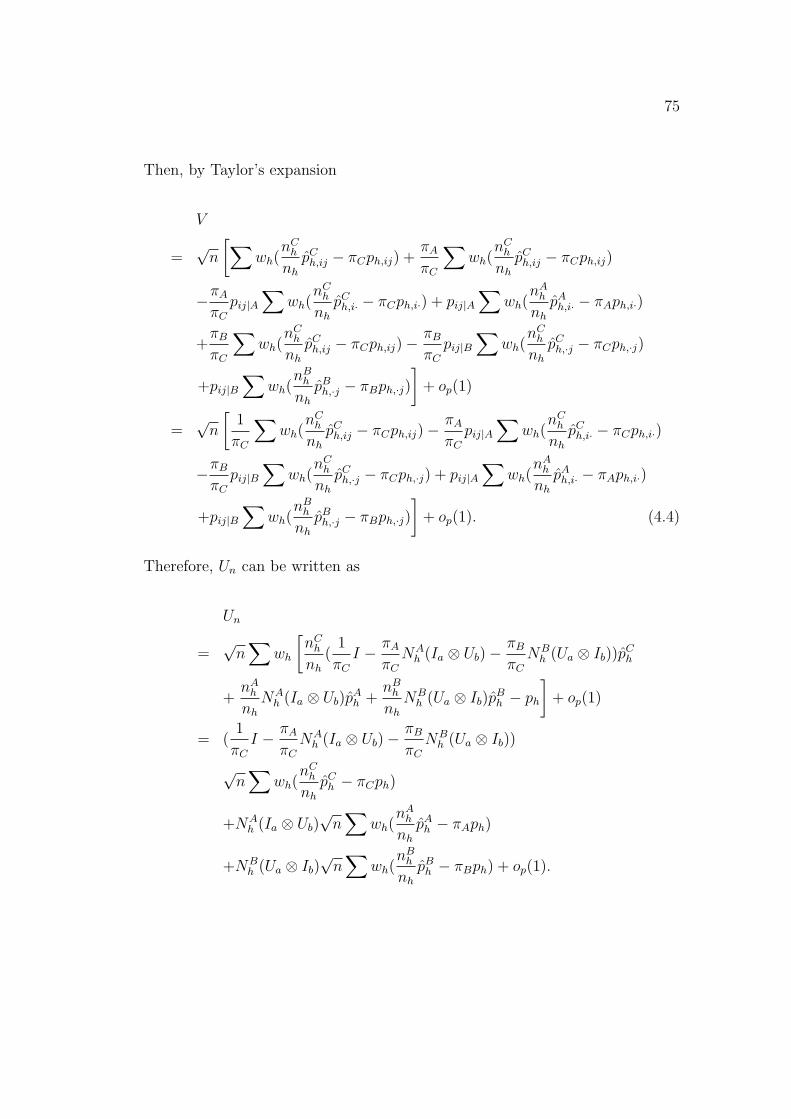
75

Then, by Taylor’s expansion

V

=√

n

[∑wh(

nCh

nh

pCh,ij − πCph,ij) +

πA

πC

∑wh(

nCh

nh

pCh,ij − πCph,ij)

−πA

πC

pij|A∑

wh(nC

h

nh

pCh,i· − πCph,i·) + pij|A

∑wh(

nAh

nh

pAh,i· − πAph,i·)

+πB

πC

∑wh(

nCh

nh

pCh,ij − πCph,ij)− πB

πC

pij|B∑

wh(nC

h

nh

pCh,·j − πCph,·j)

+pij|B∑

wh(nB

h

nh

pBh,·j − πBph,·j)

]+ op(1)

=√

n

[1

πC

∑wh(

nCh

nh

pCh,ij − πCph,ij)− πA

πC

pij|A∑

wh(nC

h

nh

pCh,i· − πCph,i·)

−πB

πC

pij|B∑

wh(nC

h

nh

pCh,·j − πCph,·j) + pij|A

∑wh(

nAh

nh

pAh,i· − πAph,i·)

+pij|B∑

wh(nB

h

nh

pBh,·j − πBph,·j)

]+ op(1). (4.4)

Therefore, Un can be written as

Un

=√

n∑

wh

[nC

h

nh

(1

πC

I − πA

πC

NAh (Ia ⊗ Ub)− πB

πC

NBh (Ua ⊗ Ib))p

Ch

+nA

h

nh

NAh (Ia ⊗ Ub)p

Ah +

nBh

nh

NBh (Ua ⊗ Ib)p

Bh − ph

]+ op(1)

= (1

πC

I − πA

πC

NAh (Ia ⊗ Ub)− πB

πC

NBh (Ua ⊗ Ib))

√n

∑wh(

nCh

nh

pCh − πCph)

+NAh (Ia ⊗ Ub)

√n

∑wh(

nAh

nh

pAh − πAph)

+NBh (Ua ⊗ Ib)

√n

∑wh(

nBh

nh

pBh − πBph) + op(1).

76

According to Lemma 3,√

n∑

wh(nC

h

nhpC

h −πCph) is asymptotically normal. Sim-

ilarly,√

n∑

wh(nA

h

nhpA

h − πAph) and√

n∑

wh(nB

h

nhpB

h − πBph) are also asymptoti-

cally normal. By the delta method, Un is also asymptotically normal.

4.4.2 Asymptotic Covariance and Estimation

In this section, we derive the explicit form of the covariance matrix of√

n(pI −p) under conditional imputation across strata with large H. An appropriate

estimator for this covariance matrix is also proposed based on the principle of

substitution.

For the sake of convenience, we first define a set of indicators.

δi·(h, k) = I{Ah,k = i}

δ·j(h, k) = I{Bh,k = j}

δA(h, k) = I{Ah,k is observed}

δB(h, k) = I{Bh,k is observed}.

According to our discussion, the asymptotic covariance matrix consists of two

components. One is the covariance of Un and the other is the expectation of

the conditional variance of Wn, where Un and Wn are defined in (4.3). Our first

task is to obtain var(Un). According to (4.4), the dth component of Un (where

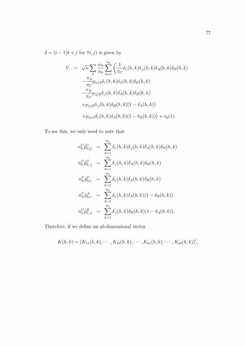
77

d = (i− 1)b + j for ∀i, j) is given by

V =√

n∑

h

wh

nh

nh∑

k=1

(1

πC

δi·(h, k)δ·j(h, k)δA(h, k)δB(h, k)

−πA

πC

pij|Aδi·(h, k)δA(h, k)δB(h, k)

−πB

πC

pij|Bδ·j(h, k)δA(h, k)δB(h, k)

+pij|Bδ·j(h, k)δB(h, k)(1− δA(h, k))

+pij|Aδi·(h, k)δA(h, k)(1− δB(h, k)))

+ op(1).

To see this, we only need to note that

nCh pC

h,ij =

nh∑

k=1

δi·(h, k)δ·j(h, k)δA(h, k)δB(h, k)

nCh pC

h,·j =

nh∑

k=1

δ·j(h, k)δA(h, k)δB(h, k)

nCh pC

h,i· =

nh∑

k=1

δi·(h, k)δA(h, k)δB(h, k)

nCh pA

h,i· =

nh∑

k=1

δi·(h, k)δA(h, k)(1− δB(h, k))

nCh pB

h,·j =

nh∑

k=1

δ·j(h, k)δB(h, k)(1− δA(h, k)).

Therefore, if we define an ab-dimensional vector

K(h, k) = (K11(h, k), · · · , K1b(h, k), · · · , Ka1(h, k), · · · , Kab(h, k))′,

78

where

Kij(h, k) =1

πC

δi·(h, k)δ·j(h, k)δA(h, k)δB(h, k)

−πA

πC

pij|Aδi·(h, k)δA(h, k)δB(h, k)

−πB

πC

pij|Bδ·j(h, k)δA(h, k)δB(h, k)

+pij|Bδ·j(h, k)δB(h, k)(1− δA(h, k))

+pij|Aδi·(h, k)δA(h, k)(1− δB(h, k)),

it follows that

Un =√

n∑

h

wh

nh

∑

k

K(h, k),

and for a given h, K(h, k), i = 1, · · · , nh are i.i.d random vectors. Consequently,

var(Un) = n∑

h

w2h

nh

Σh .= Σ1,

where Σh = cov(K(h)). This immediately implies a consistent estimator for Σ1,

which is given by Σ1 is given by

Σ1 = n∑

h

w2h

nh

Σh,

where Σh is the sample covariance matrix of

K(h, k) = (K11(h, k), · · · , K1b(h, k), · · · , Ka1(h, k), · · · , Kab(h, k))′,

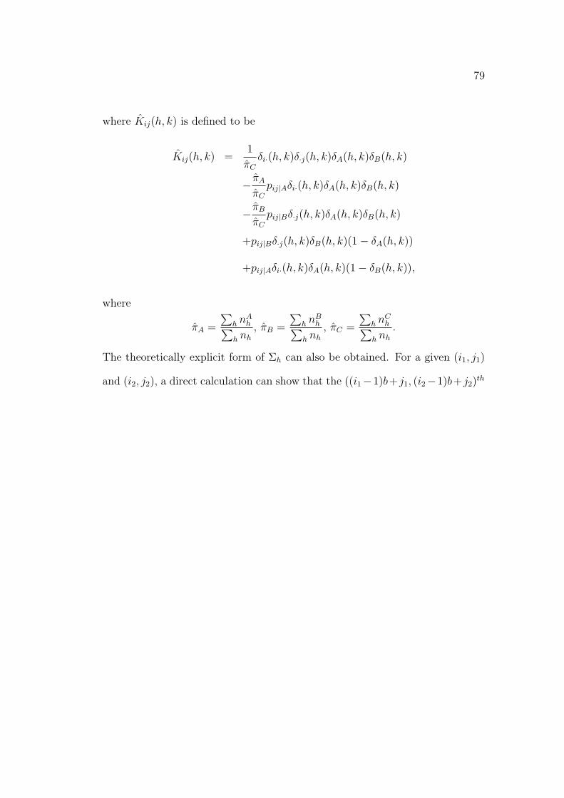
79

where Kij(h, k) is defined to be

Kij(h, k) =1

πC

δi·(h, k)δ·j(h, k)δA(h, k)δB(h, k)

− πA

πC

pij|Aδi·(h, k)δA(h, k)δB(h, k)

− πB

πC

pij|Bδ·j(h, k)δA(h, k)δB(h, k)

+pij|Bδ·j(h, k)δB(h, k)(1− δA(h, k))

+pij|Aδi·(h, k)δA(h, k)(1− δB(h, k)),

where

πA =

∑h nA

h∑h nh

, πB =

∑h nB

h∑h nh

, πC =

∑h nC

h∑h nh

.

The theoretically explicit form of Σh can also be obtained. For a given (i1, j1)

and (i2, j2), a direct calculation can show that the ((i1−1)b+ j1, (i2−1)b+ j2)th

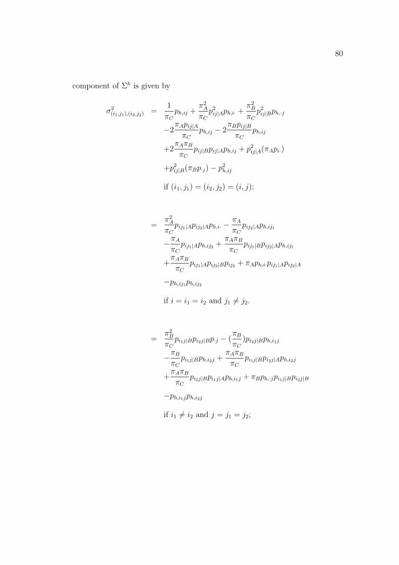
80

component of Σh is given by

σ2(i1,j1),(i2,j2) =

1

πC

ph,ij +π2

A

πC

p2ij|Aph,i· +

π2B

πC

p2ij|Bph,·j

−2πApij|A

πC

ph,ij − 2πBpij|B

πC

ph,ij

+2πAπB

πC

pij|Bpij|Aph,ij + p2ij|A(πApi·)

+p2ij|B(πBp·j)− p2

h,ij

if (i1, j1) = (i2, j2) = (i, j);

=π2

A

πC

pij1|Apij2|Aph,i· − πA

πC

pij2|Aph,ij1

−πA

πC

pij1|Aph,ij2 +πAπB

πC

pij1|Bpij2|Aph,ij1

+πAπB

πC

pij1|Apij2|Bpij2 + πAph,i·pij1|Apij2|A

−ph,ij1ph,ij2

if i = i1 = i2 and j1 6= j2.

=π2

B

πC

pi1j|Bpi2j|Bp·j − (πB

πC

)pi2j|Bph,i1j

−πB

πC

pi1j|Bph,i2j +πAπB

πC

pi1j|Bpi2j|Aph,i2j

+πAπB

πC

pi2j|Bpi1j|Aph,i1j + πBph,·jpi1j|Bpi2j|B

−ph,i1jph,i2j

if i1 6= i2 and j = j1 = j2;

81

= −ph,i1j1ph,i2j2

if i1 6= i2 and j1 6= j2.

Then we can consider the expectation of the conditional variance of Wn. Recall

that in the definition of Wn, it can be seen that

E(var(Wn|σ(C))) = ΣA + ΣB,

where

ΣA = E

(var(

√n

∑wh

nAh pA

h

nh

|σ(C))

)

ΣB = E

(var(

√n

∑wh

nBh pB

h

nh

|σ(C))

).

Then for a given (i1, j1) and (i2, j2), the [(i1 − 1)b + j1] and [(i2 − 1)b + j2]th

component of

√n

∑wh

nAh pA

h

nh

is given by

√n

∑wh

nAh,i1·(n

Ah,i1j1

/nAh,i1·)

nh

and√

n∑

wh

nAh,i2·(n

Ah,i2j2

/nAh,i2·)

nh

.

Note that, given σ(C) (the observed units), nAh,i1· and nA

h,i2· are fixed. In-

stead, (nAh,i1j1

/nAh,i1·) and (nA

h,i2j2/nA

h,i2·) have variance (pi1j1|A − p2i1j1|A)/nA

h,i1·

and (pi2j2|A − p2i2j2|A)/nA

h,i2·, respectively. Also note that their covariance is

given by −pi1j|Api2j|A/nAh,i· if i1 = i2 = i, and 0 if i1 6= i2. Therefore, the

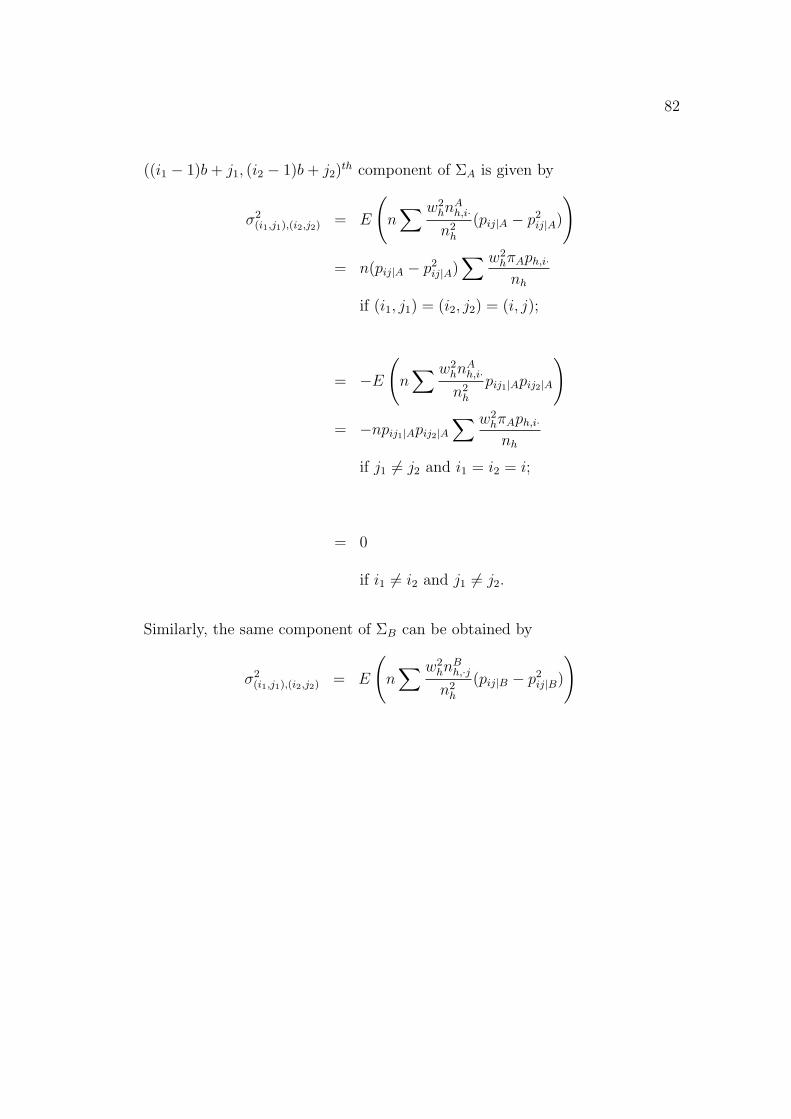
82

((i1 − 1)b + j1, (i2 − 1)b + j2)th component of ΣA is given by

σ2(i1,j1),(i2,j2) = E

(n

∑ w2hn

Ah,i·

n2h

(pij|A − p2ij|A)

)

= n(pij|A − p2ij|A)

∑ w2hπAph,i·

nh

if (i1, j1) = (i2, j2) = (i, j);

= −E

(n

∑ w2hn

Ah,i·

n2h

pij1|Apij2|A

)

= −npij1|Apij2|A∑ w2

hπAph,i·nh

if j1 6= j2 and i1 = i2 = i;

= 0

if i1 6= i2 and j1 6= j2.

Similarly, the same component of ΣB can be obtained by

σ2(i1,j1),(i2,j2) = E

(n

∑ w2hn

Bh,·j

n2h

(pij|B − p2ij|B)

)

83

= n(pij|B − p2ij|B)

∑ w2hπBph,·j

nh

if (i1, j1) = (i2, j2) = (i, j);

= −E

(n

∑ w2hn

Bh,·j

n2h

pi1j|Bpi2j|B

)

= −npi1j|Bpi2j|B∑ w2

hπBph,·jnh

if i1 6= i2 and j1 = j2 = j;

= 0

if j1 6= j2 and j1 6= j2.

The consistent estimator for ΣA and ΣB can be obtained by replacing πAph,ij

and πBph,ij by their unbiased estimators nAh,ij/nh and nB

h,ij/nh, respectively.

84

Chapter 5

Simulation Study Under

Stratified Sampling

5.1 Introduction

In the previous chapter, we have studied the asymptotic properties of cell prob-

ability estimators under various conditional imputation methods for stratified

sampling. In this chapter, extensive simulations are carried out to evaluate the

finite sample performance of the test statistics obtained in the previous chapter.

In Section 5.2, we study the test statistics obtained under the method of

imputation within stratum. In Section 5.3, we study the test statistics obtained

under the method of imputation across strata when H is small. In Section

5.4, we study the asymptotic results obtained under the method of imputation

across strata when H is large. In each section, the finite sample performances

of the Wald type test and the Rao type test for goodness-of-fit are evaluated in

terms of its empirical size.

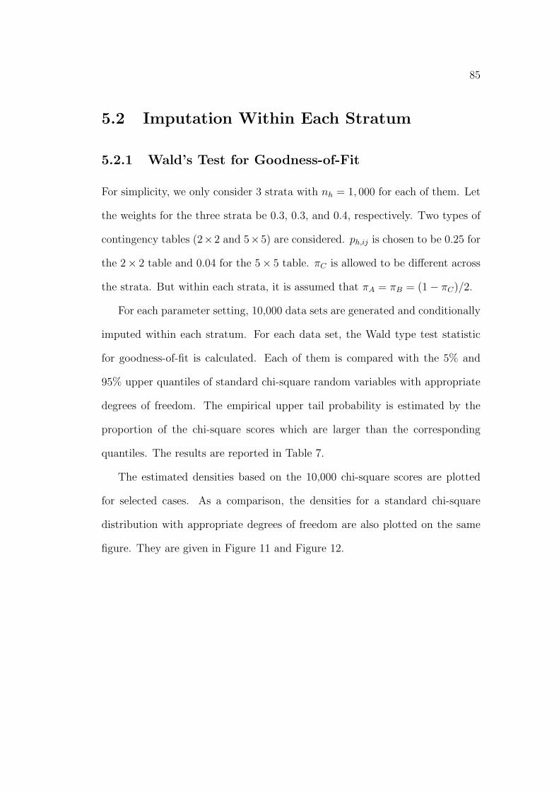
85

5.2 Imputation Within Each Stratum

5.2.1 Wald’s Test for Goodness-of-Fit

For simplicity, we only consider 3 strata with nh = 1, 000 for each of them. Let

the weights for the three strata be 0.3, 0.3, and 0.4, respectively. Two types of

contingency tables (2×2 and 5×5) are considered. ph,ij is chosen to be 0.25 for

the 2× 2 table and 0.04 for the 5× 5 table. πC is allowed to be different across

the strata. But within each strata, it is assumed that πA = πB = (1− πC)/2.

For each parameter setting, 10,000 data sets are generated and conditionally

imputed within each stratum. For each data set, the Wald type test statistic

for goodness-of-fit is calculated. Each of them is compared with the 5% and

95% upper quantiles of standard chi-square random variables with appropriate

degrees of freedom. The empirical upper tail probability is estimated by the

proportion of the chi-square scores which are larger than the corresponding

quantiles. The results are reported in Table 7.

The estimated densities based on the 10,000 chi-square scores are plotted

for selected cases. As a comparison, the densities for a standard chi-square

distribution with appropriate degrees of freedom are also plotted on the same

figure. They are given in Figure 11 and Figure 12.

86

5.2.2 Rao’s Test for Goodness-of-Fit

In this section, simulation is performed to evaluate the performance of the Rao

type test for goodness-of-fit. We use the same parameter setting as the previous

section. B, the number of bootstrap samples, is set to be 100. Due the intensity

of computation, the number of iterations is decreased to 500. The results about

the empirical upper tail probability are reported in Table 8.

The estimated densities based on 500 corrected chi-square scores are plotted

for selected cases. As a comparison, the densities for a standard chi-square

distribution with appropriate degrees of freedom are also plotted on the same

figure. They are given in Figure 13 and Figure 14

5.3 Imputation Across Strata with Small H

5.3.1 Wald’s Test for Goodness-of-Fit

In this section, simulation is used to study the finite sample performance of the

Wald test based on the method of imputation across strata. We continue to use

the same parameter setting as the previous section. The simulation is based

on 10,000 iterations and the empirical upper tail probabilities are reported in

Table 9.

The estimated densities based on the 10,000 corrected chi-square scores are

plotted for selected cases. As a comparison, the densities for a standard chi-

square distribution with appropriate degrees of freedom are also plotted on the

87

same figure. They are given in Figure 15 and Figure 16.

5.3.2 Rao’s Test for Goodness-of-Fit

In this section, the simulations concern the finite sample performance of the

Rao test based on the method of imputation across strata. We continue to use

the same parameter setting as the previous section. B, the number of bootstrap

samples, is set to be 100. The simulation is based on 500 iterations and the

empirical upper tail probabilities are reported in Table 10.

The estimated densities based on the 500 corrected chi-square scores are

plotted for selected cases. As a comparison, the densities for the appropriate

standard chi-square distribution are also plotted on the same figure. They are

given in Figure 17 and Figure 18

5.4 Imputation Across Strata with Large H

In this section, simulation is carried out to study the finite sample performance

of the Wald test for goodness-of-fit with large H. In this simulation study, H

is set to be 1000 and nh = 4, wh = 0.001. ph,ij is set to be 1/(ab), where

(a, b) = (2, 2) or (5, 5). 10,000 iterations are performed for each parameter

setting. The results are reported in Table 11.

The estimated densities based on the 10,000 scores are plotted for selected

cases. As a comparison, the densities for a standard chi-square distribution with

88

appropriate degrees of freedom are also plotted on the same figure. They are

given in Figure 19 and Figure 20

5.5 Conclusion

For the selected sample sizes and parameters, our simulation results show that

the empirical distribution of all the Wald type statistics can be well approxi-

mated by the derived asymptotic distributions.

In addition, the simulation demonstrates that the empirical distributions of

all the Rao type statistics can be well approximated by standard chi-square

distributions with appropriate degrees of freedom.

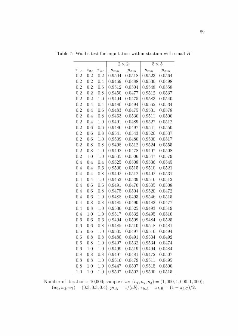
89

Table 7: Wald’s test for imputation within stratum with small H

2× 2 5× 5π1,c π2,c π3,c p0.95 p0.05 p0.95 p0.05

0.2 0.2 0.2 0.9504 0.0518 0.9523 0.05640.2 0.2 0.4 0.9469 0.0488 0.9530 0.04980.2 0.2 0.6 0.9512 0.0504 0.9548 0.05580.2 0.2 0.8 0.9450 0.0477 0.9512 0.05370.2 0.2 1.0 0.9494 0.0475 0.9583 0.05400.2 0.4 0.4 0.9480 0.0494 0.9562 0.05340.2 0.4 0.6 0.9483 0.0475 0.9531 0.05780.2 0.4 0.8 0.9463 0.0530 0.9511 0.05000.2 0.4 1.0 0.9491 0.0489 0.9527 0.05120.2 0.6 0.6 0.9486 0.0497 0.9541 0.05500.2 0.6 0.8 0.9541 0.0543 0.9520 0.05370.2 0.6 1.0 0.9509 0.0480 0.9500 0.05170.2 0.8 0.8 0.9498 0.0512 0.9524 0.05550.2 0.8 1.0 0.9492 0.0478 0.9497 0.05080.2 1.0 1.0 0.9505 0.0506 0.9547 0.05790.4 0.4 0.4 0.9525 0.0508 0.9536 0.05450.4 0.4 0.6 0.9500 0.0515 0.9510 0.05210.4 0.4 0.8 0.9492 0.0512 0.9492 0.05310.4 0.4 1.0 0.9453 0.0539 0.9516 0.05120.4 0.6 0.6 0.9491 0.0470 0.9505 0.05080.4 0.6 0.8 0.9475 0.0504 0.9520 0.04720.4 0.6 1.0 0.9488 0.0493 0.9546 0.05150.4 0.8 0.8 0.9485 0.0490 0.9483 0.04770.4 0.8 1.0 0.9536 0.0525 0.9493 0.05190.4 1.0 1.0 0.9517 0.0532 0.9495 0.05100.6 0.6 0.6 0.9494 0.0509 0.9484 0.05250.6 0.6 0.8 0.9485 0.0510 0.9518 0.04810.6 0.6 1.0 0.9505 0.0497 0.9516 0.04940.6 0.8 0.8 0.9480 0.0491 0.9504 0.04920.6 0.8 1.0 0.9497 0.0532 0.9534 0.04740.6 1.0 1.0 0.9499 0.0519 0.9494 0.04840.8 0.8 0.8 0.9497 0.0481 0.9472 0.05070.8 0.8 1.0 0.9516 0.0479 0.9511 0.04950.8 1.0 1.0 0.9447 0.0507 0.9515 0.05001.0 1.0 1.0 0.9507 0.0502 0.9500 0.0515

Number of iterations: 10,000; sample size: (n1, n2, n3) = (1, 000, 1, 000, 1, 000);(w1, w2, w3) = (0.3, 0.3, 0.4); ph,ij = 1/(ab); πh,A = πh,B = (1− πh,C)/2.

90

Table 8: Rao’s test for imputation within stratum with small H

2× 2 5× 5π1,c π2,c π3,c p0.95 p0.05 p0.95 p0.05

0.2 0.2 0.2 0.944 0.074 0.944 0.0380.2 0.2 0.4 0.940 0.038 0.938 0.0600.2 0.2 0.6 0.950 0.066 0.972 0.0680.2 0.2 0.8 0.924 0.060 0.952 0.0560.2 0.2 1.0 0.946 0.060 0.956 0.0740.2 0.4 0.4 0.944 0.050 0.954 0.0520.2 0.4 0.6 0.944 0.048 0.946 0.0660.2 0.4 0.8 0.958 0.062 0.956 0.0720.2 0.4 1.0 0.918 0.058 0.964 0.0500.2 0.6 0.6 0.950 0.048 0.942 0.0580.2 0.6 0.8 0.946 0.062 0.932 0.0860.2 0.6 1.0 0.928 0.050 0.936 0.0780.2 0.8 0.8 0.962 0.066 0.952 0.0400.2 0.8 1.0 0.940 0.056 0.950 0.0680.2 1.0 1.0 0.944 0.082 0.958 0.0680.4 0.4 0.4 0.940 0.064 0.940 0.0580.4 0.4 0.6 0.928 0.052 0.940 0.0600.4 0.4 0.8 0.942 0.072 0.960 0.0600.4 0.4 1.0 0.954 0.064 0.956 0.0640.4 0.6 0.6 0.956 0.050 0.952 0.0440.4 0.6 0.8 0.928 0.044 0.952 0.0740.4 0.6 1.0 0.964 0.048 0.950 0.0520.4 0.8 0.8 0.942 0.060 0.956 0.0540.4 0.8 1.0 0.954 0.038 0.932 0.0440.4 1.0 1.0 0.956 0.056 0.956 0.0460.6 0.6 0.6 0.950 0.072 0.942 0.0520.6 0.6 0.8 0.944 0.062 0.938 0.0660.6 0.6 1.0 0.950 0.052 0.956 0.0540.6 0.8 0.8 0.962 0.054 0.928 0.0440.6 0.8 1.0 0.948 0.038 0.958 0.0600.6 1.0 1.0 0.950 0.052 0.958 0.0400.8 0.8 0.8 0.952 0.056 0.936 0.0580.8 0.8 1.0 0.944 0.046 0.942 0.0660.8 1.0 1.0 0.950 0.066 0.970 0.0541.0 1.0 1.0 0.958 0.060 0.962 0.054

Number of iterations: 500; number of bootstrap samples: 100; sample size:(n1, n2, n3) = (1, 000, 1, 000, 1, 000); (w1, w2, w3) = (0.3, 0.3, 0.4); ph,ij = 1/(ab);

πh,A = πh,B = (1− πh,C)/2.

91

Table 9: Wald’s test for imputation across strata with small H

2× 2 5× 5π1,c π2,c π3,c p0.95 p0.05 p0.95 p0.05

0.2 0.2 0.2 0.9468 0.0493 0.9512 0.05010.2 0.2 0.4 0.9474 0.0522 0.9524 0.04980.2 0.2 0.6 0.9470 0.0507 0.9524 0.04990.2 0.2 0.8 0.9500 0.0477 0.9512 0.05050.2 0.2 1.0 0.9493 0.0456 0.9520 0.05500.2 0.4 0.4 0.9551 0.0510 0.9509 0.04760.2 0.4 0.6 0.9541 0.0496 0.9521 0.04990.2 0.4 0.8 0.9476 0.0513 0.9493 0.05160.2 0.4 1.0 0.9480 0.0528 0.9498 0.05120.2 0.6 0.6 0.9514 0.0517 0.9515 0.05250.2 0.6 0.8 0.9508 0.0487 0.9503 0.05230.2 0.6 1.0 0.9505 0.0508 0.9503 0.05040.2 0.8 0.8 0.9494 0.0529 0.9531 0.04820.2 0.8 1.0 0.9471 0.0472 0.9511 0.05010.2 1.0 1.0 0.9498 0.0529 0.9513 0.05900.4 0.4 0.4 0.9484 0.0506 0.9519 0.05100.4 0.4 0.6 0.9473 0.0488 0.9488 0.04990.4 0.4 0.8 0.9504 0.0522 0.9521 0.04860.4 0.4 1.0 0.9502 0.0479 0.9517 0.05150.4 0.6 0.6 0.9501 0.0495 0.9488 0.05140.4 0.6 0.8 0.9529 0.0455 0.9454 0.04630.4 0.6 1.0 0.9486 0.0516 0.9532 0.05100.4 0.8 0.8 0.9519 0.0478 0.9513 0.04910.4 0.8 1.0 0.9471 0.0494 0.9476 0.04710.4 1.0 1.0 0.9481 0.0496 0.9503 0.05220.6 0.6 0.6 0.9501 0.0492 0.9520 0.04900.6 0.6 0.8 0.9556 0.0506 0.9496 0.05430.6 0.6 1.0 0.9492 0.0481 0.9565 0.05170.6 0.8 0.8 0.9498 0.0512 0.9509 0.04770.6 0.8 1.0 0.9493 0.0539 0.9483 0.04840.6 1.0 1.0 0.9498 0.0498 0.9472 0.04270.8 0.8 0.8 0.9497 0.0498 0.9510 0.04900.8 0.8 1.0 0.9513 0.0489 0.9503 0.05130.8 1.0 1.0 0.9503 0.0500 0.9499 0.04901.0 1.0 1.0 0.9514 0.0494 0.9501 0.0505

Number of iterations: 10,000; sample size: (n1, n2, n3) = (1, 000, 1, 000, 1, 000);(w1, w2, w3) = (0.3, 0.3, 0.4); ph,ij = 1/(ab); πh,A = πh,B = (1− πh,C)/2.

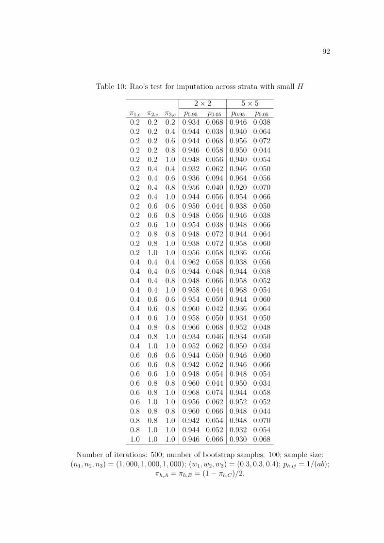
92

Table 10: Rao’s test for imputation across strata with small H

2× 2 5× 5π1,c π2,c π3,c p0.95 p0.05 p0.95 p0.05

0.2 0.2 0.2 0.934 0.068 0.946 0.0380.2 0.2 0.4 0.944 0.038 0.940 0.0640.2 0.2 0.6 0.944 0.068 0.956 0.0720.2 0.2 0.8 0.946 0.058 0.950 0.0440.2 0.2 1.0 0.948 0.056 0.940 0.0540.2 0.4 0.4 0.932 0.062 0.946 0.0500.2 0.4 0.6 0.936 0.094 0.964 0.0560.2 0.4 0.8 0.956 0.040 0.920 0.0700.2 0.4 1.0 0.944 0.056 0.954 0.0660.2 0.6 0.6 0.950 0.044 0.938 0.0500.2 0.6 0.8 0.948 0.056 0.946 0.0380.2 0.6 1.0 0.954 0.038 0.948 0.0660.2 0.8 0.8 0.948 0.072 0.944 0.0640.2 0.8 1.0 0.938 0.072 0.958 0.0600.2 1.0 1.0 0.956 0.058 0.936 0.0560.4 0.4 0.4 0.962 0.058 0.938 0.0560.4 0.4 0.6 0.944 0.048 0.944 0.0580.4 0.4 0.8 0.948 0.066 0.958 0.0520.4 0.4 1.0 0.958 0.044 0.968 0.0540.4 0.6 0.6 0.954 0.050 0.944 0.0600.4 0.6 0.8 0.960 0.042 0.936 0.0640.4 0.6 1.0 0.958 0.050 0.934 0.0500.4 0.8 0.8 0.966 0.068 0.952 0.0480.4 0.8 1.0 0.934 0.046 0.934 0.0500.4 1.0 1.0 0.952 0.062 0.950 0.0340.6 0.6 0.6 0.944 0.050 0.946 0.0600.6 0.6 0.8 0.942 0.052 0.946 0.0660.6 0.6 1.0 0.948 0.054 0.948 0.0540.6 0.8 0.8 0.960 0.044 0.950 0.0340.6 0.8 1.0 0.968 0.074 0.944 0.0580.6 1.0 1.0 0.956 0.062 0.952 0.0520.8 0.8 0.8 0.960 0.066 0.948 0.0440.8 0.8 1.0 0.942 0.054 0.948 0.0700.8 1.0 1.0 0.944 0.052 0.932 0.0541.0 1.0 1.0 0.946 0.066 0.930 0.068

Number of iterations: 500; number of bootstrap samples: 100; sample size:(n1, n2, n3) = (1, 000, 1, 000, 1, 000); (w1, w2, w3) = (0.3, 0.3, 0.4); ph,ij = 1/(ab);

πh,A = πh,B = (1− πh,C)/2.

93

Table 11: Wald’s test for imputation across strata with large H

2× 2 5× 5πC πA πB p0.95 p0.05 p0.95 p0.05

1.0 0.0 0.0 0.050 0.952 0.054 0.9550.9 0.0 0.1 0.048 0.948 0.050 0.9460.8 0.0 0.2 0.048 0.951 0.051 0.9470.8 0.1 0.1 0.049 0.949 0.042 0.9180.7 0.0 0.3 0.046 0.945 0.048 0.9350.7 0.1 0.2 0.049 0.945 0.042 0.9150.7 0.2 0.1 0.046 0.947 0.042 0.9280.6 0.0 0.4 0.045 0.946 0.053 0.9460.6 0.1 0.3 0.047 0.946 0.043 0.9130.6 0.2 0.2 0.045 0.948 0.043 0.9260.5 0.0 0.5 0.043 0.946 0.054 0.9350.5 0.1 0.4 0.045 0.950 0.048 0.9070.5 0.2 0.3 0.048 0.949 0.042 0.9230.4 0.0 0.6 0.045 0.946 0.059 0.9400.4 0.1 0.5 0.048 0.951 0.050 0.9060.4 0.2 0.4 0.052 0.948 0.049 0.9220.4 0.3 0.3 0.052 0.952 0.043 0.9210.3 0.0 0.7 0.050 0.951 0.062 0.9450.3 0.1 0.6 0.048 0.948 0.055 0.9090.3 0.2 0.5 0.053 0.953 0.050 0.9300.3 0.3 0.4 0.058 0.953 0.047 0.9260.3 0.4 0.3 0.057 0.952 0.044 0.9200.2 0.0 0.8 0.045 0.945 0.078 0.9480.2 0.1 0.7 0.050 0.949 0.062 0.9240.2 0.2 0.6 0.059 0.951 0.056 0.9260.2 0.3 0.5 0.064 0.953 0.057 0.9290.2 0.4 0.4 0.067 0.953 0.055 0.9230.1 0.0 0.9 0.054 0.947 0.132 0.9590.1 0.1 0.8 0.060 0.950 0.102 0.9360.1 0.2 0.7 0.084 0.955 0.102 0.9340.1 0.3 0.6 0.106 0.959 0.103 0.9310.1 0.4 0.5 0.115 0.960 0.093 0.930

Number of iterations: 10,000; nh = 4; H = 1, 000; wh = 0.001; ph,ij = 1/(ab).

94

Figure 11: Empirical density for Wald’s statistic based on 2× 2 tables

0 2 4 6 8 10

0.00

0.05

0.10

0.15

0.20

0.25

χ2−score

Den

sity

(π1,cπ2,cπ3,c) = (0.2,0.4,0.6)

empiricaltheoretical

0 2 4 6 8 10

0.00

0.05

0.10

0.15

0.20

0.25

χ2−score

Den

sity

(π1,cπ2,cπ3,c) = (0.3,0.5,0.3)

0 2 4 6 8 10

0.00

0.05

0.10

0.15

0.20

0.25

χ2−score

Den

sity

(π1,cπ2,cπ3,c) = (0.4,0.3,0.5)

0 2 4 6 8 10

0.00

0.05

0.10

0.15

0.20

0.25

χ2−score

Den

sity

(π1,cπ2,cπ3,c) = (0.5,0.4,0.4)

Number of iterations: 10,000; sample size: (n1, n2, n3) = (1, 000, 1, 000, 1, 000);(w1, w2, w3) = (0.3, 0.3, 0.4); ph,ij = 0.25; πh,A = πh,B = (1− πh,C)/2.

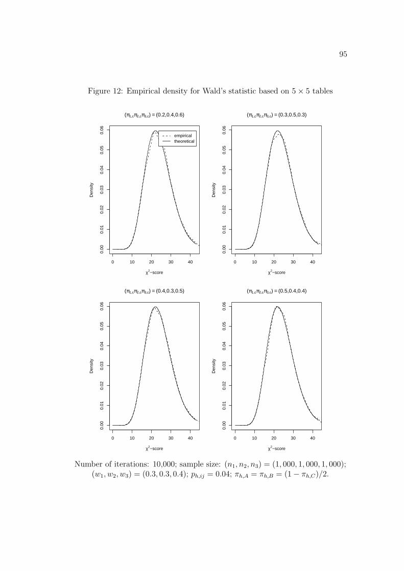
95

Figure 12: Empirical density for Wald’s statistic based on 5× 5 tables

0 10 20 30 40

0.00

0.01

0.02

0.03

0.04

0.05

0.06

χ2−score

Den

sity

(π1,cπ2,cπ3,c) = (0.2,0.4,0.6)

empiricaltheoretical

0 10 20 30 40

0.00

0.01

0.02

0.03

0.04

0.05

0.06

χ2−score

Den

sity

(π1,cπ2,cπ3,c) = (0.3,0.5,0.3)

0 10 20 30 40

0.00

0.01

0.02

0.03

0.04

0.05

0.06

χ2−score

Den

sity

(π1,cπ2,cπ3,c) = (0.4,0.3,0.5)

0 10 20 30 40

0.00

0.01

0.02

0.03

0.04

0.05

0.06

χ2−score

Den

sity

(π1,cπ2,cπ3,c) = (0.5,0.4,0.4)

Number of iterations: 10,000; sample size: (n1, n2, n3) = (1, 000, 1, 000, 1, 000);(w1, w2, w3) = (0.3, 0.3, 0.4); ph,ij = 0.04; πh,A = πh,B = (1− πh,C)/2.

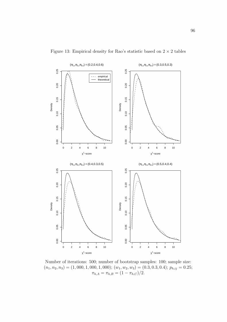
96

Figure 13: Empirical density for Rao’s statistic based on 2× 2 tables

0 2 4 6 8 10

0.00

0.05

0.10

0.15

0.20

0.25

χ2−score

Den

sity

(π1,cπ2,cπ3,c) = (0.2,0.4,0.6)

empiricaltheoretical

0 2 4 6 8 10

0.00

0.05

0.10

0.15

0.20

0.25

χ2−score

Den

sity

(π1,cπ2,cπ3,c) = (0.3,0.5,0.3)

0 2 4 6 8 10

0.00

0.05

0.10

0.15

0.20

0.25

χ2−score

Den

sity

(π1,cπ2,cπ3,c) = (0.4,0.3,0.5)

0 2 4 6 8 10

0.00

0.05

0.10

0.15

0.20

0.25

χ2−score

Den

sity

(π1,cπ2,cπ3,c) = (0.5,0.4,0.4)

Number of iterations: 500; number of bootstrap samples: 100; sample size:(n1, n2, n3) = (1, 000, 1, 000, 1, 000); (w1, w2, w3) = (0.3, 0.3, 0.4); ph,ij = 0.25;

πh,A = πh,B = (1− πh,C)/2.

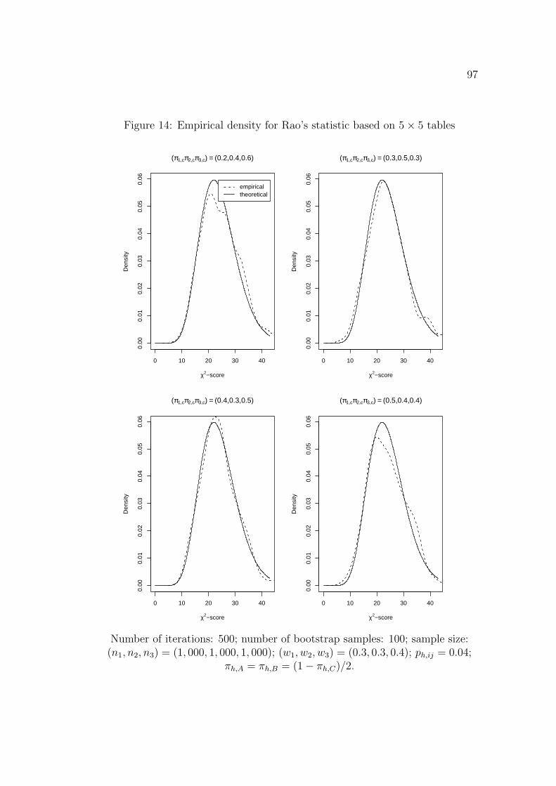
97

Figure 14: Empirical density for Rao’s statistic based on 5× 5 tables

0 10 20 30 40

0.00

0.01

0.02

0.03

0.04

0.05

0.06

χ2−score

Den

sity

(π1,cπ2,cπ3,c) = (0.2,0.4,0.6)

empiricaltheoretical

0 10 20 30 40

0.00

0.01

0.02

0.03

0.04

0.05

0.06

χ2−score

Den

sity

(π1,cπ2,cπ3,c) = (0.3,0.5,0.3)

0 10 20 30 40

0.00

0.01

0.02

0.03

0.04

0.05

0.06

χ2−score

Den

sity

(π1,cπ2,cπ3,c) = (0.4,0.3,0.5)

0 10 20 30 40

0.00

0.01

0.02

0.03

0.04

0.05

0.06

χ2−score

Den

sity

(π1,cπ2,cπ3,c) = (0.5,0.4,0.4)

Number of iterations: 500; number of bootstrap samples: 100; sample size:(n1, n2, n3) = (1, 000, 1, 000, 1, 000); (w1, w2, w3) = (0.3, 0.3, 0.4); ph,ij = 0.04;

πh,A = πh,B = (1− πh,C)/2.

98

Figure 15: Empirical density for Wald’s statistic based on 2 × 2 tables withsmall H

0 2 4 6 8 10

0.00

0.05

0.10

0.15

0.20

0.25

χ2−score

Den

sity

(π1,cπ2,cπ3,c) = (0.2,0.4,0.6)

empiricaltheoretical

0 2 4 6 8 10

0.00

0.05

0.10

0.15

0.20

0.25

χ2−score

Den

sity

(π1,cπ2,cπ3,c) = (0.3,0.5,0.3)

0 2 4 6 8 10

0.00

0.05

0.10

0.15

0.20

0.25

χ2−score

Den

sity

(π1,cπ2,cπ3,c) = (0.4,0.3,0.5)

0 2 4 6 8 10

0.00

0.05

0.10

0.15

0.20

0.25

χ2−score

Den

sity

(π1,cπ2,cπ3,c) = (0.5,0.4,0.4)

Number of iterations: 10,000; sample size: (n1, n2, n3) = (1, 000, 1, 000, 1, 000);(w1, w2, w3) = (0.3, 0.3, 0.4); ph,ij = 0.25; πh,A = πh,B = (1− πh,C)/2.

99

Figure 16: Empirical density for Wald’s statistic based on 5 × 5 tables withsmall H

0 10 20 30 40

0.00

0.01

0.02

0.03

0.04

0.05

0.06

χ2−score

Den

sity

(π1,cπ2,cπ3,c) = (0.2,0.4,0.6)

empiricaltheoretical

0 10 20 30 40

0.00

0.01

0.02

0.03

0.04

0.05

0.06

χ2−score

Den

sity

(π1,cπ2,cπ3,c) = (0.3,0.5,0.3)

0 10 20 30 40

0.00

0.01

0.02

0.03

0.04

0.05

0.06

χ2−score

Den

sity

(π1,cπ2,cπ3,c) = (0.4,0.3,0.5)

0 10 20 30 40

0.00

0.01

0.02

0.03

0.04

0.05

0.06

χ2−score

Den

sity

(π1,cπ2,cπ3,c) = (0.5,0.4,0.4)

Number of iterations: 10,000; sample size: (n1, n2, n3) = (1, 000, 1, 000, 1, 000);(w1, w2, w3) = (0.3, 0.3, 0.4); ph,ij = 0.04; πh,A = πh,B = (1− πh,C)/2.

100

Figure 17: Empirical density for Rao’s statistic based on 2×2 tables with smallH

0 2 4 6 8 10

0.00

0.05

0.10

0.15

0.20

0.25

χ2−score

Den

sity

(π1,cπ2,cπ3,c) = (0.2,0.4,0.6)

empiricaltheoretical

0 2 4 6 8 10

0.00

0.05

0.10

0.15

0.20

0.25

χ2−score

Den

sity

(π1,cπ2,cπ3,c) = (0.3,0.5,0.3)

0 2 4 6 8 10

0.00

0.05

0.10

0.15

0.20

0.25

χ2−score

Den

sity

(π1,cπ2,cπ3,c) = (0.4,0.3,0.5)

0 2 4 6 8 10

0.00

0.05

0.10

0.15

0.20

0.25

χ2−score

Den

sity

(π1,cπ2,cπ3,c) = (0.5,0.4,0.4)

Number of iterations: 500; number of bootstrap samples: 100; sample size:(n1, n2, n3) = (1, 000, 1, 000, 1, 000); (w1, w2, w3) = (0.3, 0.3, 0.4); ph,ij = 0.25;

πh,A = πh,B = (1− πh,C)/2.

101

Figure 18: Empirical density for Rao’s statistic based on 5×5 tables with smallH

0 10 20 30 40

0.00

0.01

0.02

0.03

0.04

0.05

0.06

χ2−score

Den

sity

(π1,cπ2,cπ3,c) = (0.2,0.4,0.6)

empiricaltheoretical

0 10 20 30 40

0.00

0.01

0.02

0.03

0.04

0.05

0.06

χ2−score

Den

sity

(π1,cπ2,cπ3,c) = (0.3,0.5,0.3)

0 10 20 30 40

0.00

0.01

0.02

0.03

0.04

0.05

0.06

χ2−score

Den

sity

(π1,cπ2,cπ3,c) = (0.4,0.3,0.5)

0 10 20 30 40

0.00

0.01

0.02

0.03

0.04

0.05

0.06

χ2−score

Den

sity

(π1,cπ2,cπ3,c) = (0.5,0.4,0.4)

Number of iterations: 500; number of bootstrap samples: 100; sample size:(n1, n2, n3) = (1, 000, 1, 000, 1, 000); (w1, w2, w3) = (0.3, 0.3, 0.4); ph,ij = 0.04;

πh,A = πh,B = (1− πh,C)/2.

102

Figure 19: Empirical density for Wald’s statistic based on 2 × 2 tables withlarge H

0 2 4 6 8 10

0.00

0.05

0.10

0.15

0.20

0.25

χ2−score

Den

sity

(πAπBπC) = (0.4,0.3,0.3)

empiricaltheoretical

0 2 4 6 8 10

0.00

0.05

0.10

0.15

0.20

0.25

χ2−score

Den

sity

(πAπBπC) = (0.2,0.4,0.4)

0 2 4 6 8 10

0.00

0.05

0.10

0.15

0.20

0.25

χ2−score

Den

sity

(πAπBπC) = (0.1,0.1,0.8)

0 2 4 6 8 10

0.00

0.05

0.10

0.15

0.20

0.25

χ2−score

Den

sity

(πAπBπC) = (0.1,0.2,0.7)

Number of iterations: 10,000; nh = 4; H = 1, 000; wh = 0.001; ph,ij = 0.25

103

Figure 20: Empirical density for Wald’s statistic based on 5 × 5 tables withlarge H

0 10 20 30 40

0.00

0.01

0.02

0.03

0.04

0.05

0.06

χ2−score

Den

sity

(πAπBπC) = (0.4,0.3,0.3)

empiricaltheoretical

0 10 20 30 40

0.00

0.01

0.02

0.03

0.04

0.05

0.06

χ2−score

Den

sity

(πAπBπC) = (0.2,0.4,0.4)

0 10 20 30 40

0.00

0.01

0.02

0.03

0.04

0.05

0.06

χ2−score

Den

sity

(πAπBπC) = (0.1,0.1,0.8)

0 10 20 30 40

0.00

0.01

0.02

0.03

0.04

0.05

0.06

χ2−score

Den

sity

(πAπBπC) = (0.1,0.2,0.7)

Number of iterations: 10,000; nh = 4; H = 1, 000; wh = 0.001; ph,ij = 0.04

104

Chapter 6

Real Data Study

6.1 The Beaver Dam Eye Study

The first example concerns data observed from the Beaver Dam Eye Study

(BDES), which is an ongoing population-based cohort study of age-related eye

disease, cataract, and maculopathy. Detailed description of the target popu-

lation and study can be found in Klein, Klein, and Linton (1992). Five-year

follow-up data have been collected and the ten-year follow-up of the cohort is

in progress.

Briefly, a private census of the population of Beaver Dam, Wisconsin (99%

white), was performed from September 15, 1987 to May 4, 1988, to identify all

residents in the city or township of Beaver Dam who were 43 to 84 years of

age. Afterward, the population was examed over a 30-month period. Of 5,925

eligible people, 4,926(83.1%) participated in the study. Photographs of each eye

were taken and graded. An examination and a standardized questionnaire were

administered.

One objective of this trial is to study the relationship of macular edema

and proteinuria, which are two common complications in people with diabetes.

105

Macular edema (absent = 0 or present = 1) is a condition in which fluid builds

up in the retina in the macular area at the back of the eye. It can cause swelling

that will seriously impair vision. Proteinuria (absent = 0 or present = 1) is the

presence of excessive protein in the urine, which is usually a symptom of kidney

malfunction. The data for macular edema are available for both eyes. However,

due to the high correlations between the left and right eyes, our analysis will be

presented for right eyes only.

Besides the two primary end points, some auxiliary variables with no missing

values are also available, e.g., sex (male = 1, female = 2). As a result, two

imputation classes are created according to sex = 1 or sex = 2. We refer to

these two classes as class 1 and class 2, respectively. In this example, the

imputation class can also be viewed as strata. Therefore, we are essentially

performing imputation within each stratum. The subjects with both primary

end points (macular edema and proteinuria) missing are simply ignored. As a

result, a reduced data set is produced. Based on the reduced data set, some

summary statistics about this data set are provided in Table 12.

Conditional imputation is then performed within each imputation class. The

summary statistics after imputation are reported in Table 13.

After conditional imputation, the cell probability estimates are obtained for

each stratum. For the purpose of comparison, the same estimates are also ob-

tained by re-weighting, which uses the complete units only. Since the sampling

weight is not available in BDES study, we assume an equal sampling weight

106

(0.5) for the two strata (female and male), which means we are assuming that

in the whole population, the number of females is approximately equal to the

number of males. The overall cell probability estimates are obtained and the

test of independence is carried out. The results are reported in Table 14. The

results indicate a strong relationship between macular edema and proteinuria.

6.2 Victimization Incidents Study

The second example comes from the victimization incidents survey conducted

by U.S. Department of Justice in 1989. The original data set contains the

information about sampling weight, sex, violence type, injury, medical care, re-

porting of incidence, and the number of offenders involved in the crime. One

of the problems of interest is to test if the sex (female and male) is related to

the number of offenders. The original data contain 2219 observations. They

are divided into two imputation classes according to violence type (violent and

nonviolent). We refer to them as class 1 and class 2. Within each imputation

class, 50 strata are created artificially by combining the units with similar sam-

pling weights. For example, there are a total of 720 observations contained in

class 1. The observations are sorted according to their sampling weights from

small to large. Then every 14 (≈ 720/50) consecutive observations are grouped

together into one strata with the last strata containing 34 observations. Then

from each strata a simple random sample of 4 observations are taken to form our

subsample. A similar procedure is also carried out for class 2. Consequently,

107

our subsample contains two imputation classes (class 1 and class 2). Each class

contains 50 strata with stratum size equal to 4. The sampling weights are also

adjusted appropriately.

There are two primary variables of interest. One is sex (female and male)

with 1 denoting male and 2 denoting female. The other one is number of of-

fenders involved in the crime (NUM) with 1 denoting only one, 2 denoting more

than one. The sex is observed for every unit, but NUM suffers an appreciable

number missing responses (with 11% missing in the original sample).

The summary statistics of the selected subsample are provided in Table 15.

The method of conditional imputation across strata is performed on the sub-

sample. The summary statistics after imputation is given in Table 16. The cell

probabilities based on the complete units only and the whole data set after im-

putation are reported in Table 17. The results indicate no relationship between

the sex and the number of offenders. The covariance matrix of the cell prob-

ability estimates are reported in Table 18. From Table 18 it can be seen that

the standard deviation of cell probability estimate after conditional imputation

is comparable to the re-weighting method and in some cases it improves the

efficiency.

108

Table 12: Summary statistics of BDES data

ProteinuriaStrata Absent Present Missing

Absent 337 51 151 Present 14 17 5

macular Missing 24 40 0edema Absent 332 50 16

2 Present 15 10 1Missing 30 26 0

Table 13: Summary statistics of BDES data after imputation

ProteinuriaStrata Absent Present

1 Absent 369 89macular Present 19 26edema 2 Absent 378 71

Present 16 15

109

Table 14: Statistical analysis of BDES data after imputation

ProteinuriaConditional Imputation Re-Weighting

Strata Absent Present Absent Present1 Absent 0.731 0.177 0.804 0.122

macular Present 0.038 0.054 0.033 0.041edema 2 Absent 0.788 0.148 0.815 0.123

Present 0.033 0.031 0.037 0.025overall Absent 0.760 0.163 0.810 0.123

Present 0.036 0.043 0.035 0.033Test Independence: χ2 = 36.01 p < 0.01 χ2 = 39.34 p < 0.01

Table 15: Summary statistics for the selected subsample

NUMclass sex 1 2 missing

1 1 44 15 202 69 21 31

2 1 83 32 22 64 18 1

Table 16: Summary statistics after imputation

NUMclass 1 2

1 1 56 23sex 2 92 29

2 1 85 322 65 18

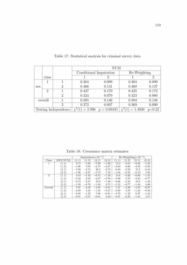
110

Table 17: Statistical analysis for criminal survey data

NUMConditional Imputation Re-Weighting

class 1 2 1 21 1 0.304 0.099 0.304 0.099

sex 2 0.466 0.131 0.460 0.1372 1 0.427 0.170 0.425 0.172

2 0.324 0.079 0.323 0.080overall 1 0.385 0.146 0.384 0.148

2 0.372 0.097 0.369 0.099Testing Independence χ2(1) = 2.996 p = 0.08345 χ2(1) = 1.4930 p=0.22

Table 18: Covariance matrix estimates

Imputation(×10−4) Re-Weighting(×10−4)Class (SEX,NUM) (1, 1) (1, 2) (2, 1) (2, 2) (1, 1) (1, 2) (2, 1) (2, 2)

1 (1, 1) 15.5 −1.66 −7.80 −1.86 12.3 −3.84 −6.83 −1.62(1, 2) −1.66 5.94 −2.74 −0.27 −3.84 6.66 −2.59 −0.23(2, 1) −7.80 −2.74 20.5 −2.72 −6.83 −2.59 15.5 −6.10(2, 2) −1.86 −0.27 −2.72 7.16 −1.62 −0.23 −6.10 7.95

2 (1, 1) 13.9 −5.43 −6.74 −1.59 13.8 −5.60 −6.66 −1.55(1, 2) −5.43 8.58 −2.37 −0.78 −5.60 8.70 −2.33 −0.77(2, 1) −6.74 −2.37 10.8 −1.38 −6.66 −2.33 10.5 −1.49(2, 2) −1.59 −0.78 −1.38 3.75 −1.55 −0.77 −1.49 3.80

Overall (1, 1) 7.91 −2.58 −3.85 −0.91 7.47 −2.90 −3.70 −0.87(1, 2) −2.58 4.45 −1.35 −0.37 −2.90 4.59 −1.32 −0.36(2, 1) −3.85 −1.35 7.08 −0.91 −3.70 −1.32 6.37 −1.34(2, 2) −0.91 −0.37 −0.91 2.46 −0.87 −0.36 −1.34 2.57

111

Bibliography

[1] Chen, J., and Shao, J. (2000). Nearest-Neighbor Imputation for Survey Data,

J. of Official Statistics, 16, 583-599.

[2] Chen, J., and Shao, J. (2001). Jackknife Variance Estimation for Nearest-

Neighbor Imputation. JASA, 96, 260-269.

[3] Durrett, Richard (1995). Probability: Theory and Examples, Duxbury Press,

New York.

[4] Lehmann, E.L. (1997). Testing Statistical Hypothesis. Springer, New York.

[5] Lehmann, E.L. (1997). Theory of Point Estimation. Springer, New York.

[6] Kalton, G. and Kasprzyk, D. (1986). The treatment of missing data. Survey

Methodology, 12, 1-16.

[7] Little, R.J. and Rubin, D.B. (1987). Statistical Analysis with Missing Data.

Wiley, New York.

[8] Rao, J.N.K. and Scott, A.J. (1987). On simple adjustments to chi-square

tests with sample survey data. Annals of Statistics, 15, 1-12.

[9] Rao, J.N.K. and Shao, J. (1992). Jackknife variance estimation with survey

data under hot deck imputation. Biometrika, 79, 811-822.

112

[10] Johnson, R. and Wichern, D. (1998). Applied Multivariate Statistical Anal-

ysis. Prentice Hall, Inc. Englewood Cliffs, N.J.

[11] Rubin, D.B. (1987). Multiple Imputation for Nonresponses in Surveys. Wi-

ley, New York.

[12] Shao, J. (1998). Mathematical Statistics. Springer, New York

[13] Shao, J. and Wang, H. (2001). Sample correlation coefficients based on

survey data under regression imputation. To appear in JASA.

[14] Schafer, J.L. (1997). Analysis of Incomplete Multivariate Data. Chapman

and Hall, London.

[15] Schenker, N. and Welsh, A.H. (1988). Asymptotic results for multiple im-

putation, Annals of Statistics, 16, No. 4. (Dec., 1988), pp. 1550-1566.

[16] Srivastava, M.S. and Carter, E.M. (1986). The maximum likelihood method

for non-response in sample surveys. Survey Methodology, 12, 61-72.

[17] Vaart, A.W. (1998). Asymptotic Statistics. Cambridge, New York.

[18] Venables, W.N. and Ripley, B.D. Modern Applied Statitics with S-Plus.

Springer, New York.