Two-Step Calibration Method for SWAT

Francisco Olivera, Ph.D.Assistant ProfessorHuidae ChoGraduate Student

Department of Civil EngineeringTexas A&M UniversityCollege Station - Texas

SWAT 2005Zurich, Switzerland

July 14th, 2005

Can we extract spatial information from

temporal data?

Francisco Olivera, Ph.D.Assistant ProfessorHuidae ChoGraduate Student

Department of Civil EngineeringTexas A&M UniversityCollege Station - Texas

SWAT 2005Zurich, Switzerland

July 14th, 2005

Objective

Given: A calibration routine that adjusts the terrain parameters independently for each sub-basin and HRU (i.e., extracts spatial information).

Hypothesis: A model that can reproduce the system’s responses for a “long” period of time has the correct parameter spatial distribution.

Lake Lewisville Watershed

Period of record: 1987 – 1999

• Four temperature stations: one inside the watershed and three outside.

• Six precipitation stations: two inside the watershed and four outside.

Area: 2500 km2

• Four flow gauging stations: one is an inlet, one is used for calibration, and two are used for (spatial) validation.

Lake Lewisville Watershed C

urve

num

ber

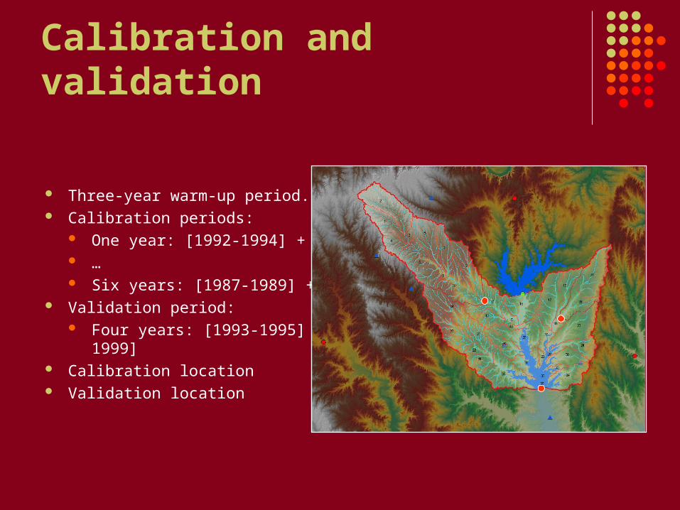
Calibration and validation

Three-year warm-up period. Calibration periods:

One year: [1992-1994] + [1995] … Six years: [1987-1989] + [1990-1995]

Validation period: Four years: [1993-1995] + [1996-1999]

Calibration location Validation location

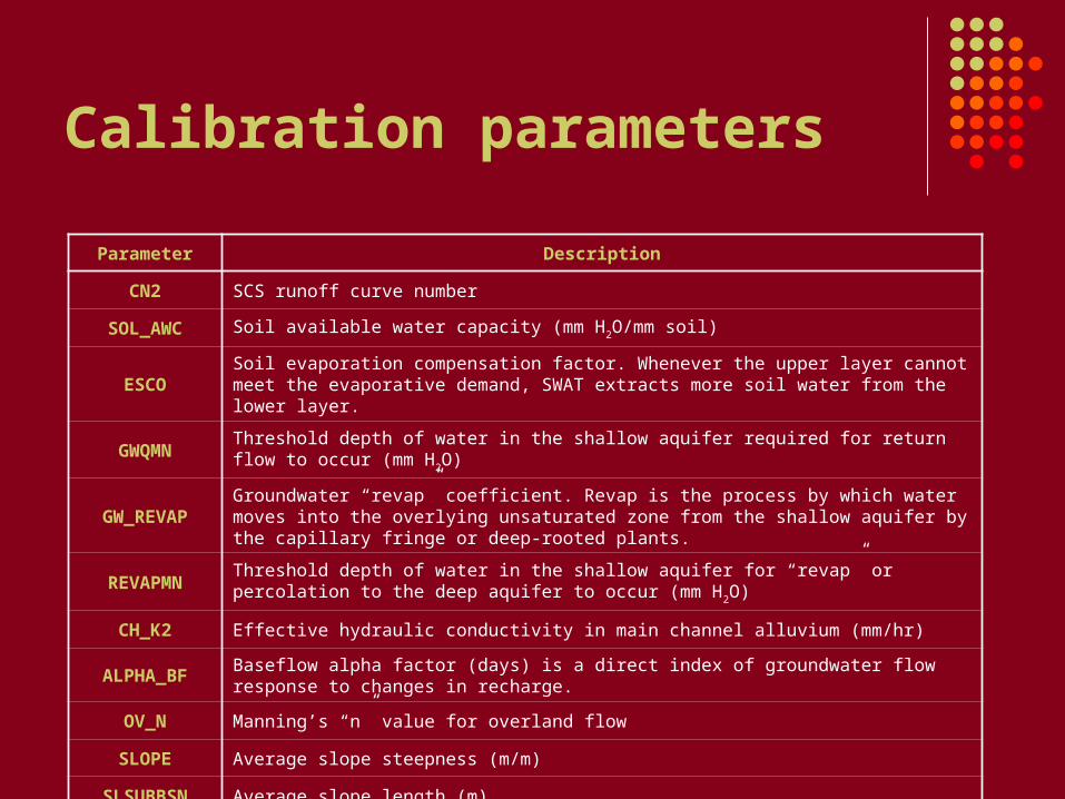
Calibration parameters

Parameter Description

CN2 SCS runoff curve number

SOL_AWC Soil available water capacity (mm H2O/mm soil)

ESCOSoil evaporation compensation factor. Whenever the upper layer cannot meet the evaporative demand, SWAT extracts more soil water from the lower layer.

GWQMN Threshold depth of water in the shallow aquifer required for return flow to occur (mm H2O)

GW_REVAPGroundwater “revap” coefficient. Revap is the process by which water moves into the overlying unsaturated zone from the shallow aquifer by the capillary fringe or deep-rooted plants.

REVAPMNThreshold depth of water in the shallow aquifer for “revap” or percolation to the deep aquifer to occur (mm H2O)

CH_K2 Effective hydraulic conductivity in main channel alluvium (mm/hr)

ALPHA_BFBaseflow alpha factor (days) is a direct index of groundwater flow response to changes in recharge.

OV_N Manning’s “n” value for overland flow

SLOPE Average slope steepness (m/m)

SLSUBBSN Average slope length (m)

Calibration levels

Watershed: All sub-basin and HRU parameters are adjusted by applying one single parameter-change rule over the entire watershed.

Sub-basin: All sub-basin and HRU parameters are adjusted by applying a different parameter-change rule in each subbasin. Follows watershed calibration.

HRU: Each HRU parameter is adjusted differently. Follows sub-basin calibration.

Method A (plus/minus): -0.05 < α < 0.05

Method B (factor): 0.9 < α < 1.1

Method C (alpha): -0.5 < α < 0.5

Parameter-change rules

i 1 i max minP P (P P )

i 1 i i minP P (P P )

i 1 i max iP P (P P )

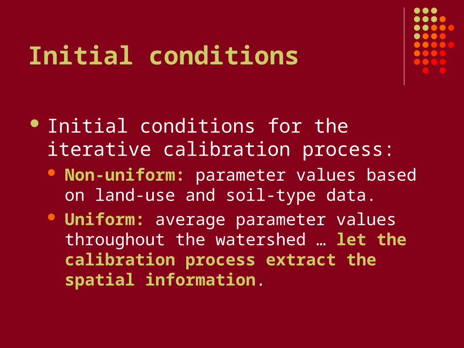
Initial conditions

Initial conditions for the iterative calibration process: Non-uniform: parameter values based on land-

use and soil-type data. Uniform: average parameter values throughout

the watershed … let the calibration process extract the spatial information.

Objective functions

Sum of the square of the residuals (SSR)

Sum of the absolute value of the residuals (SAR)

No logQ or Q in the denominator was used because some flows were zero.

2simulated observedSSR (Q Q )

simulated observedSSR Q Q

Model efficiency

Model efficiency was evaluated with the Nash-Sutcliffe coefficient:

where is the long-term flow average (i.e., the predicted flows with “no model”).

2simulated observed

2 2observed observed

(Q Q ) SSRNS 1 1

(Q Q ) (Q Q )

Q

Hydrologic unitC

alib

ratio

n //

SS

R /

/ D

istr

ibut

ed

// P

lus-

min

us /

/ 4

2

The increase in NS between subbasin and watershed is small, and between HRU and subbasin is negligible.

0.00

0.10

0.20

0.30

0.40

0.50

0.60

0.70

0.80

0.90

1.00

1 2 3 4 5 6

Number of years used in calibration

Na

sh-S

utc

liffe

co

effi

cien

t

SGPHGPWGPWGP

Hydrologic unitV

alid

atio

n //

SS

R /

/ D

istr

ibut

ed /

/ P

lus-

min

us /

/ 42

The decrease in NS between subbasin and watershed is small, and between HRU and subbasin is negligible.

0.00

0.10

0.20

0.30

0.40

0.50

0.60

0.70

0.80

0.90

1.00

1 2 3 4 5 6

Number of years used in calibration

Na

sh-S

utc

liffe

co

effi

cien

t

SGPHGPWGPWGP

Objective functionC

alib

ratio

n //

Dis

trib

uted

//

Plu

s-m

inus

//

42

The increase in NS between subbasin and watershed is small, and between HRU and subbasin is negligible.

0.00

0.10

0.20

0.30

0.40

0.50

0.60

0.70

0.80

0.90

1.00

1 2 3 4 5 6

Number of years used in calibration

Na

sh-S

utc

liff

e c

oe

ffic

ien

t

SGPHGPWGPWGP

0.0

0.1

0.2

0.3

0.4

0.5

0.6

0.7

0.8

0.9

1.0

1 2 3 4 5 6

Number of years used in calibration

Nas

h-S

utc

liffe

co

effi

cien

t

SGP

HGP

WGP

SSR

SAR

0.00

0.10

0.20

0.30

0.40

0.50

0.60

0.70

0.80

0.90

1.00

1 2 3 4 5 6

Number of years used in calibration

Nas

h-S

utc

liffe

co

effi

cien

t

SGP

HGP

WGP

WGP

Objective functionV

alid

atio

n //

Dis

trib

uted

//

Plu

s-m

inu

s //

42

The increase in NS between subbasin and watershed is small, and between HRU and subbasin is negligible.

SSR

SAR0.0

0.1

0.2

0.3

0.4

0.5

0.6

0.7

0.8

0.9

1.0

1 2 3 4 5 6

Number of years used in calibration

Nas

h-S

utc

liffe

co

effi

cien

tSGP

HGP

WGP

Parameter change functionC

alib

ratio

n //

SS

R /

/ D

istr

ibut

ed

// 4

2

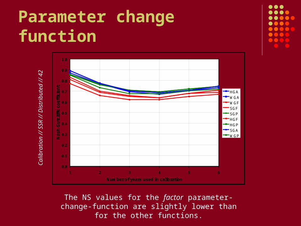
The NS values for the factor parameter-change-function are slightly lower than for the other functions.

0.0

0.1

0.2

0.3

0.4

0.5

0.6

0.7

0.8

0.9

1.0

1 2 3 4 5 6

Number of years used in calibration

Nas

h-S

utc

liffe

co

effi

cien

t

HGAWGAWGFSGFSGPHGFHGPSGAWGP

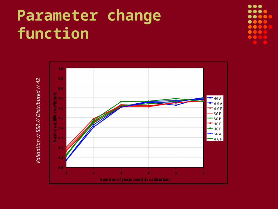
Parameter change functionV

alid

atio

n //

SS

R /

/ D

istr

ibut

ed /

/ 42

0.0

0.1

0.2

0.3

0.4

0.5

0.6

0.7

0.8

0.9

1.0

1 2 3 4 5 6

Number of years used in calibration

Nas

h-S

utc

liffe

co

effi

cien

t

HGAWGAWGFSGFSGPHGFHGPSGAWGP

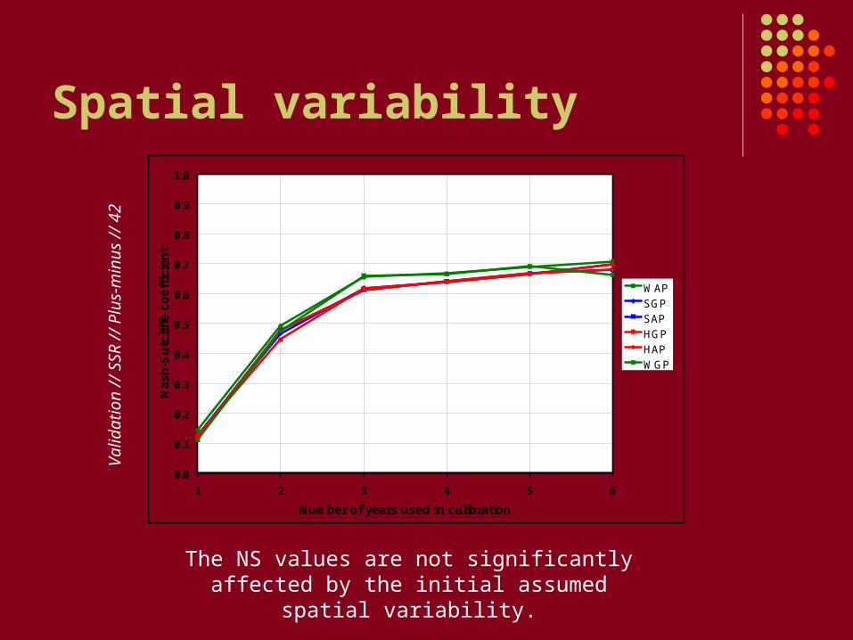
Spatial variabilityC

alib

ratio

n //

SS

R /

/ P

lus-

min

us /

/ 42

The NS values are not significantly affected by the initial assumed spatial variability.

0.0

0.1

0.2

0.3

0.4

0.5

0.6

0.7

0.8

0.9

1.0

1 2 3 4 5 6

Number of years used in calibration

Na

sh-S

utc

liffe

co

effi

cie

nt

WAPSGPSAPHGPHAPWGP

Hydrographs - CalibrationC

alib

ratio

n //

SS

R /

/ P

lus-

min

us /

/ 42

The simulated hydrographs are fundamentally equal even though the initial conditions before

the calibration were very different.

0

50

100

150

200

250

1/1/1990 1/1/1991 1/1/1992 12/31/1992 12/31/1993 12/31/1994

Flo

w (

m3/s

) HGP

WAP

WGP

Observed

Parameter valuesS

SR

//

Ave

rage

//

Plu

s-m

inus

//

HR

U

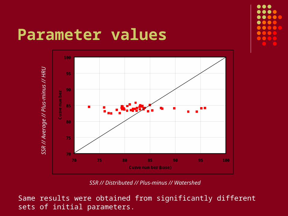
Same results were obtained from significantly different sets of initial parameters.

70

75

80

85

90

95

100

70 75 80 85 90 95 100

Curve number (base)

Cu

rve

nu

mb

er

SSR // Distributed // Plus-minus // Watershed

Spatial variabilityV

alid

atio

n //

SS

R /

/ P

lus-

min

us /

/ 4

2

The NS values are not significantly affected by the initial assumed spatial variability.

0.0

0.1

0.2

0.3

0.4

0.5

0.6

0.7

0.8

0.9

1.0

1 2 3 4 5 6

Number of years used in calibration

Na

sh-S

utc

liffe

co

effi

cie

nt

WAPSGPSAPHGPHAPWGP

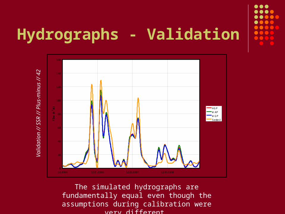
Hydrographs - ValidationV

alid

atio

n //

SS

R /

/ P

lus-

min

us /

/ 4

2

The simulated hydrographs are fundamentally equal even though the assumptions during

calibration were very different.

0

20

40

60

80

100

120

140

160

1/1/1996 12/31/1996 12/31/1997 12/31/1998

Flo

w (

m3/s

) HGP

WAP

WGP

Series1

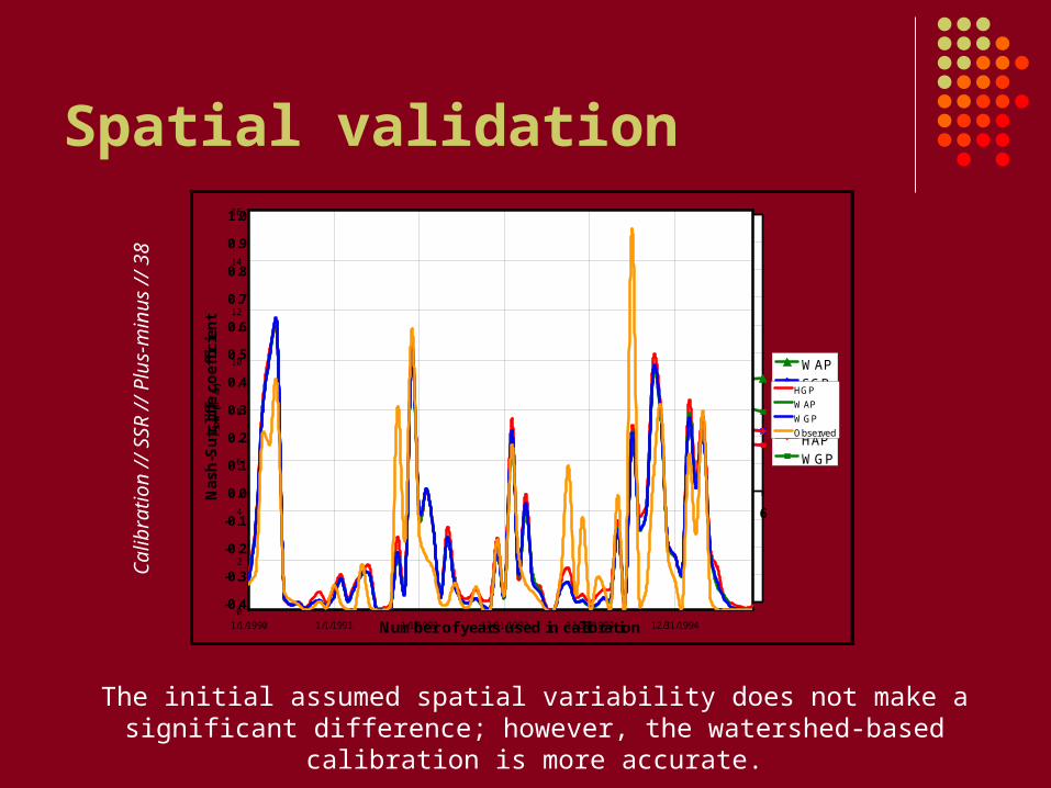
Spatial validationC

alib

ratio

n //

SS

R /

/ P

lus-

min

us /

/ 38

The initial assumed spatial variability does not make a significant difference; however, the watershed-based calibration is more accurate.

-0.4

-0.3

-0.2

-0.1

0.0

0.1

0.2

0.3

0.4

0.5

0.6

0.7

0.8

0.9

1.0

1 2 3 4 5 6

Number of years used in calibration

Na

sh-S

utc

liffe

co

effi

cien

t

WAPSGPSAPHGPHAPWGP

0

2

4

6

8

10

12

14

16

1/1/1990 1/1/1991 1/1/1992 12/31/1992 12/31/1993 12/31/1994

Flo

w (

m3/s

) HGP

WAP

WGP

Observed

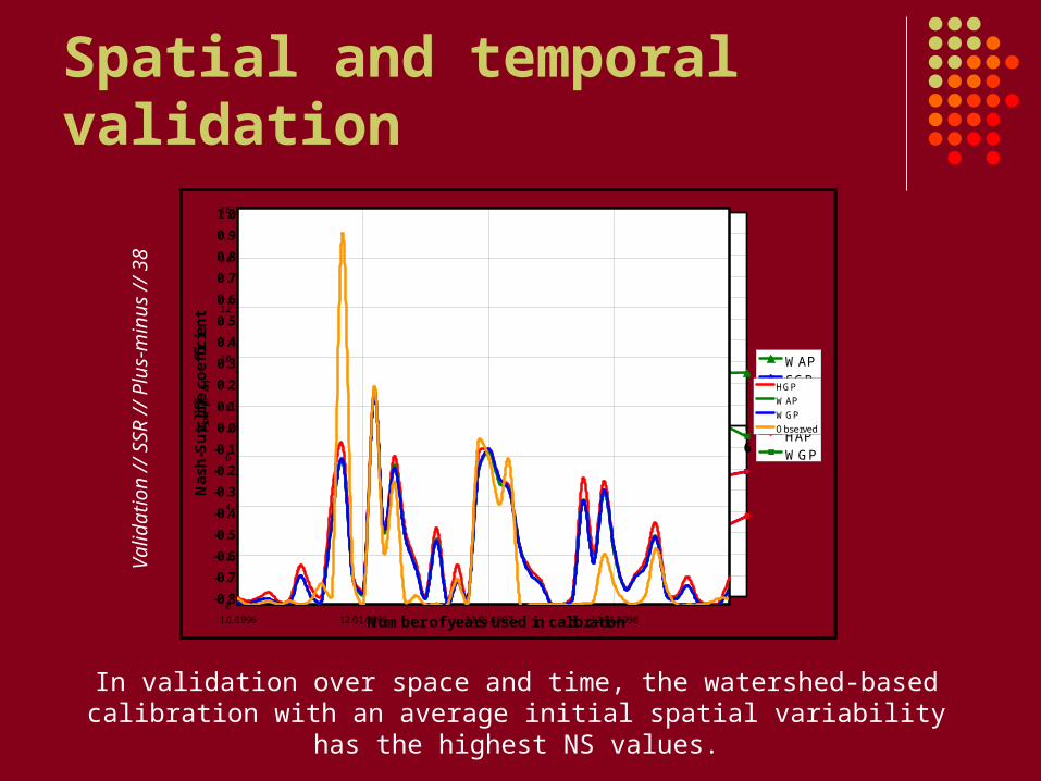
Spatial and temporal validationV

alid

atio

n //

SS

R /

/ P

lus-

min

us /

/ 3

8

In validation over space and time, the watershed-based calibration with an average initial spatial variability has the highest NS values.

-0.8

-0.7

-0.6

-0.5

-0.4

-0.3

-0.2

-0.1

0.0

0.1

0.2

0.3

0.4

0.5

0.6

0.7

0.8

0.9

1.0

1 2 3 4 5 6

Number of years used in calibration

Na

sh-S

utc

liffe

co

effi

cien

t

WAPSGPSAPHGPHAPWGP

0

2

4

6

8

10

12

14

16

1/1/1996 12/31/1996 12/31/1997 12/31/1998

Flo

w (

m3/s

) HGP

WAP

WGP

Observed

Spatial validationC

alib

ratio

n //

SS

R /

/ P

lus-

min

us /

/ 37

Not even the watershed-based calibration using the spatial variability defined by the soil and land use data produces a good NS value.

-3.0

-2.5

-2.0

-1.5

-1.0

-0.5

0.0

0.5

1.0

1 2 3 4 5 6

Number of years used in calibration

Na

sh-S

utc

liffe

co

effi

cien

t

WAPSGPSAPHGPHAPWGP

0

10

20

30

40

50

60

70

80

1/1/1990 1/1/1991 1/1/1992 12/31/1992 12/31/1993 12/31/1994

Flo

w (

m3/s

) HGP

WAP

WGP

Observed

Spatial and temporal validationV

alid

atio

n //

SS

R /

/ P

lus-

min

us /

/ 3

7

-1.5

-1.0

-0.5

0.0

0.5

1.0

1 2 3 4 5 6

Number of years used in calibration

Na

sh-S

utc

liffe

co

effi

cien

t

WAPSGPSAPHGPHAPWGP

Not even the watershed-based calibration using the spatial variability defined by the soil and land use data produces a good NS value.

0

5

10

15

20

25

30

35

40

1/1/1996 12/31/1996 12/31/1997 12/31/1998

Flo

w (

m3/s

) HGP

WAP

WGP

Observed

Discussions

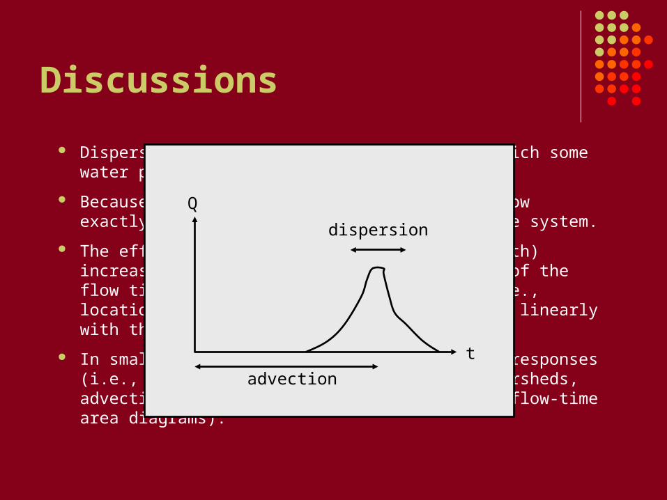
Dispersion is the hydrodynamic process by which some water particles flow faster than others.

Because of dispersion, it is difficult to know exactly when and where a particle entered the system.

The effect of dispersion (i.e., response width) increases proportionally to the square root of the flow time; while the effect of advection (i.e., location of the response centroid) increases linearly with the flow time.

In small watersheds, dispersion “mixes” all responses (i.e., unit hydrograph); while in large watersheds, advection keeps responses “separate” (i.e., flow-time area diagrams).

t

Q

dispersion

advection

Conclusions

It was not possible to “extract hydrologic information from temporal data” for the 2,500-km2 Lake Lewisville watershed.

The effect of the spatial variability was small compared to the effect of hydrodynamic dispersive processes in the system.

The number of years used for calibrating the model was fundamental for determining the parameter values.

The parameter-change rule and the selected objective function did not significantly affect the calibration process.

Questions?