two simple methods for improving a triangle mesh surface

Volume 0 (1981), Number 0 pp. 1–12 COMPUTER GRAPHICS forum

Two Simple Methods for Improving a Triangle Mesh Surface

Robert J. Renka

Department of Computer Science & Engineering, University of North Texas, Denton, TX, [email protected]

AbstractWe present two simple and efficient local methods that reposition vertices of a triangle mesh surface with the goalof producing good triangle shapes while preserving the enclosed volume and sharp features. The methods involveminimizing a quadratic energy functional with respect to variations in a tangent plane (or in the direction of acrease) at each free vertex. One of the methods is aimed at producing uniform angles, while the other methodis designed to produce uniform triangle areas, or more generally, to force relative triangle areas to conform tocurvature estimates or estimates of local feature size so that vertex density is low in flat spots and relatively high inregions of large curvature. Test results demonstrate the effectiveness of both methods, especially when combined.

Keywords: mesh improvement, mesh smoothing, surface mesh, feature-preserving

Categories and Subject Descriptors (according to ACM CCS): I.3.5 [Computer Graphics]: Computational Geometryand Object Modeling—Curve, surface, solid, and object representations

1. Introduction

In [REN15] we introduced two new mesh smoothing meth-ods and demonstrated their efficiency and effectiveness rel-ative to several alternative methods for treating planar trian-gulations. Here we extend the methods to surface meshes.

In the context of a finite element mesh the term smooth-ing refers to the process of repositioning vertices in order toimprove element shapes as defined by aspect ratio, smallestangle, largest angle, or some other quality measure. In thecase of a surface mesh the direction of vertex motion mayhave both a tangential component corresponding to repa-rameterization, and a normal component corresponding to achange in geometry, and the term smoothing refers to both.The goal is to improve element shape with tangential motion,and to remove noise with normal motion. Our focus here ison the former. We assume that noise removal, if necessary,has been applied in a preprocessing step, and the surfacerepresented by the input mesh is piecewise smooth. Referto [DMS*99], [WY11], [GYH13], and [HS13] for examplesof methods that include denoising.

We also assume that the number of vertices is fixed, butwe allow for changes in connection topology via edge flipschosen to enforce the local Delaunay angle criterion: the pairof angles opposite each interior edge sum to at most 180 de-grees. In the case of a pair of nonplanar triangles, a Delaunay

edge flip reduces surface area [DZM07]. The change in ge-ometry, however, is not significant unless the mesh is verycoarse. We alternate enforcement of the Delaunay angle cri-terion with one or more smoothing sweeps in which eachfree vertex is repositioned with the remaining vertex posi-tions fixed.

An alternative to mesh smoothing is remeshing basedon the Delaunay refinement paradigm with bounded tri-angle aspect ratios [DR10, CDS13]. Mesh smoothing pro-vides no quality guarantees, but it can produce excellent re-sults very quickly without insertion of additional vertices.It makes optimal use of the vertices, eliminating the inef-ficiency of overrefinement. It also extends to quadrilateralsand to anisotropic meshes. (Refer to [ZS00], [LL03], and[ZBX09] for examples.)

In order to preserve the shape and volume of the sur-face, vertex motion is constrained as follows. The surfacemay have any number of boundary curves whose verticesare fixed. During each smoothing sweep an interior vertexmay be categorized as a corner, which is not free to move, ora crease vertex, which is constrained to move along a line.The remaining vertices are constrained to move in a tan-gent plane whose normal is computed by normalizing thetriangle-area weighted sum of the normals to the trianglesthat contain the vertex. We employ the sharp feature detec-

c© 2015 The Author(s)Computer Graphics Forum c© 2015 The Eurographics Association and JohnWiley & Sons Ltd. Published by John Wiley & Sons Ltd.

Robert J. RenkaDepartment of Computer Science & Engineering, University of North Texas, Denton, TX, [email protected] / Two Simple Methods for Improving a Triangle Mesh Surface

tion method of [PSK*02] for categorizing vertices. This isthe same method used by [GYH13].

The central idea in our smoothing method is to minimizea least squares functional consisting of a weighted sum ofsquared triangle areas, where the triangles are those that con-tain the vertex to be repositioned. For the planar case it wasshown in [REN15] that, to the extent allowed by the con-straint vertices, the weighted triangle areas in the smoothedmesh are identical. Constant weights therefore result in uni-form triangle areas. More generally a pair of triangles hasarea ratio equal to the reciprocal of the weight ratio so thatlarge weight corresponds to small area and high vertex den-sity. In a finite element mesh the weights might, for example,be chosen on the basis of error estimates. Surprisingly, it isalso possible to choose the weights so that angles are uni-form, resulting in an angle-based method that more directlyproduces well-shaped triangles.

The uniformity of weighted triangle areas extends to a tri-angle mesh surface, and in a typical application is less likelyto be constrained by a complex boundary. The weights inthe angle-based method are identical to those in the planarcase. In the area-based method the weights may be cho-sen on the basis of estimated curvature or local feature sizewhich tends to be inversely related to curvature. More pre-cisely, triangle weights are computed by averaging vertexdensities, where a vertex density is either the reciprocal ofthe squared local feature size or an approximation to themaximum normal curvature constrained by upper and lowerbounds. The local feature size at a vertex is taken to be thedistance from the vertex to the medial axis. We employ themethod of [ABK98] for approximating the distance to themedial axis by the distance to the nearest pole — the nearerof the two Voronoi vertices, one on each side of the surface,farthest from the vertex in the 3D Voronoi region centered atthe vertex.

Compared with the method presented here, the methodof [SG03] uses a much more elaborate scheme for preserv-ing surface shape and volume, involving overlapping lo-cal parameterizations, and includes more options for chang-ing mesh connection topology, but is quite similar in thatit employs both area-based and angle-based smoothing (us-ing methods introduced in [SG02]). The difference betweensmoothing methods is further discussed in the next section.

Our methods are described in detail in Section 2, test re-sults are discussed in Section 3, and Section 4 concludes thepaper.

2. Methods

We assume as input to our algorithm a list of vertices in R3

and one or more additional data structures, such as a trianglelist with consistently ordered vertex indices and neighboringtriangle indices, that define the connection topology and al-low us to distinguish between a fixed boundary vertex and

an interior vertex which may have zero, one, or two degreesof freedom, depending on its categorization. The algorithmconsists of a loop around the following three steps

1. Compute triangle weights (in the case of area-basedsmoothing with non-constant weight).

2. Apply one or more smoothing sweeps.3. Apply edge flips (unless volume is to be preserved).

The loop is terminated either by reaching an upper bound onthe number of iterations or when no edge flips occur and themaximum displacement of a vertex is bounded by a toler-ance.

A smoothing sweep consists of a loop in which each inte-rior vertex is categorized and relocated (unless categorizedas a corner) with the remaining vertex locations fixed. Theorder in which vertices are processed is the (arbitrary) or-der in which they are stored in the input array. Let v0 de-note the position of an interior vertex with the cyclically-ordered sequence of neighboring vertices vk : k = 1, . . . ,nwith vn+1 = v1. Denote by v a new position to be computed,and for k = 1 to n, let τk(v) be the triangle with vertices v,vk, and vk+1, normal vector

Ak(v) = (vk−v)× (vk+1−v),

and area ‖Ak(v)‖/2. We define a tangent plane at v0 by theunit normal computed from the area-weighted sum of nor-mals to the triangles containing v0:

n =n

∑k=1

Ak(v0) normalized to a unit vector. (1)

The surface normal n is not well-defined if v0 and all itsneighbors coincide, in which case v is set to v0.

Note, however, that the position of v0 may be altered ina subsequent sweep after one or more of its neighbors havebeen moved. It was observed in [GYH13] that, while nottrue for motion along a crease, a perturbation of v0 in thetangent plane defined by n preserves the volume bounded bythe surface. It should be noted that the proof of this theo-rem includes an erroneous statement, but it is not difficult torepair the proof, and the theorem is valid as shown in Ap-pendix A. Also, volume can be preserved by motion along acrease by projecting the crease direction onto the orthogonalcomplement of n.

Theorem 1 Vertex displacement in the tangent plane definedby Equation (1) preserves the volume bounded by the surface(and a cone connecting the boundary, if any, to the origin).

As previously mentioned edge flips result in smallchanges in volume and are therefore not permitted if volumeis to be preserved. It is generally not necessary, however, topreserve the exact volume of the input mesh, and our test-ing revealed little sensitivity of mesh quality to the choiceof vertex normals. In particular the eigenvector associatedwith the dominant eigenvalue of the matrix that represents

c© 2015 The Author(s)Computer Graphics Forum c© 2015 The Eurographics Association and John Wiley & Sons Ltd.


the local structure tensor (defined in Section 2.1) is a viablealternative to (1).

We describe the vertex categorization method in the firstsubsection below. We define the linear least squares systemand show that it has a unique solution in Section 2.2. Weexplain the uniformity by proving a result for smooth para-metric surfaces in Section 2.3. In Section 2.4 we discuss thechoice of weights, and we treat changes in connection topol-ogy in the last subsection.

2.1. Vertex Categorization

This subsection describes the means by which we restrict themotion of vertices in order to preserve shape. In the processof computing the normal n at v0 we also compute a matrixT representing a local structure tensor:

T =n

∑k=1

ωknknTk ,

where nk is the unit normal to triangle τk(v0). We useweights suggested by [PSK*02]:

ωk =‖Ak(v0)‖

Amaxexp(−gk

σ

),

where Amax is twice the area of the largest triangle in themesh, gk is the distance from v0 to the barycenter of triangleτk(v0), and σ is the average edge length in the mesh.

Since T is a symmetric positive semi-definite order-3 ma-trix it has nonnegative real eigenvalues which may be or-dered as λ1 ≥ λ2 ≥ λ3 ≥ 0 with corresponding orthonormaleigenvectors u1,u2, and u3. Note that, for i = 1,2,3,

λi = uTi T ui =

n

∑k=1

ωk(nTk ui)

2

so that λi is the ω-weighted sum of the squares of the pro-jections of nk onto direction ui. The basic idea behind thecategorization scheme is the following. Two relatively smalleigenvalues indicates a smooth surface with a well-definednormal direction u1 and little variance in the triangle nor-mals. If λ3 is the only small eigenvalue, then the normalstend to vary in a plane normal to a crease or ridge in the u3direction. If there are no small eigenvalues then there is nopreferred orientation, indicating a corner vertex. The vertexis categorized according to the maximum of the followingmeasures of saliency:

surface patch: S2 = λ1−λ2crease: εS1 = ε(λ2−λ3)corner: εηS0 = εηλ3

where ε and η are nonnegative constants that define a bal-ance between noise tolerance and crease/corner detection.Following the recommendation of [PSK*02], we set bothconstants to 2. The minimum detectable dihedral crease an-

gle β satisfies

tanβ

2=

√1

ε+1

so that, with ε = 2, angles of 60 degrees or more are cate-gorized as creases. With η = 2 the same angle distinguishesbetween a crease and a corner.

2.2. Vertex Relocation

The heart of the smoothing method is a constrained linearleast squares problem. Here we show that it can be treatedby solving a linear system with a symmetric positive definitematrix of order 2. The quadratic least squares functional is

φ(v) =12

n

∑k=1

wk‖Ak(v)‖2, (2)

where wk is a weight associated with triangle τk(v0). It wasobserved in [XHG*12] that, with wk = 1 for all k, minimiz-ing φ is equivalent to minimizing the variance in trianglearea. However, that observation does not apply to the caseof non-constant weights. The area-based method of [SG03]includes weights that control triangle area ratios, but thatmethod is not as simple and efficient as the new method pre-sented here. Let ek = vk+1− vk be the edge opposite v intriangle τk(v) so that Ak(v) = ek× (v−vk). The gradient ofφ at v is

∇φ(v) =n

∑k=1

wkAk(v)× ek

=n

∑k=1

wk[ek× (v−vk)× ek]

=n

∑k=1

wkrk(v−vk), (3)

where rk is the linear operator defined by

rk(w) = ek×w× ek

= ‖ek‖2w−〈w,ek〉ek.

Suppose v0 is a crease vertex with crease direction (unitvector) e0 computed as the eigenvector associated with thesmallest eigenvalue of T . Then v is constrained to move onlyin the direction e0:

v = v0 + se0,

where s is defined by setting the partial derivative of φ withrespect to s to zero:

〈∇φ(v),e0〉 = 〈n

∑k=1

wkrk(v0−vk + se0),e0〉

=n

∑k=1

wk[〈rk(v0−vk),e0〉+ s〈rk(e0),e0〉]

= 0.



We thus obtain

s = ∑nk=1 wk〈rk(vk−v0),e0〉

∑nk=1(‖ek‖2−〈e0,ek〉2)

.

Now consider the case that v0 has two degrees of freedom.We obtain a unit vector e1 in the tangent plane by normal-izing the projection of one of the edges vk− v0 onto the or-thogonal complement of n. Define e2 = n× e1, and let

v = v0 + s1e1 + s2e2. (4)

We then have

rk(v−vk) = rk(v0−vk)+ s1rk(e1)+ s2rk(e2).

We obtain an order-2 linear system by zeroing the partialderivatives of φ with respect to the coefficients s1 and s2:

〈∇φ(v),e1〉 =n

∑k=1

wk[〈rk(v0−vk),e1〉+

s1〈rk(e1),e1〉+ s2〈rk(e2),e1〉] = 0

and

〈∇φ(v),e2〉 =n

∑k=1

wk[〈rk(v0−vk),e2〉+

s1〈rk(e1),e2〉+ s2〈rk(e2),e2〉] = 0.

Define

h =n

∑k=1

wk‖ek‖2

a =n

∑k=1

wk〈ek,e2〉2

b =n

∑k=1

wk〈ek,e1〉〈ek,e2〉

c =n

∑k=1

wk〈ek,e1〉2

f1 =n

∑k=1

wk〈rk(vk−v0),e1〉

f2 =n

∑k=1

wk〈rk(vk−v0),e2〉

Then by the Pythagorean theorem, h = a+c, and the systemis As = f for

A =(

h− c −b−b h−a

)=(

a −b−b c

),

The following theorem, proved in Appendix B, shows thatthe new position v is uniquely defined.

Theorem 2 A is positive definite.

2.3. Smooth Parametric Surfaces

In order to understand why minimizers of the least squaresfunctional defined by Equation (2) tend to have uniformweighted triangle area, we treat the triangle mesh surface as

a discrete approximation to a smooth parametric surface. Fora free vertex v0, denote by C the closed polygonal curve de-fined by the sequence of 1-ring neighbors vk : k = 1, . . . ,n,and let

S = f ∈C2(Ω,R3) : f1× f2 6= 0 and f|∂Ω = C

for Ω = [0,1]2, where f1 and f2 denote first partial deriva-tives. The image of an element of S is a regular parametricsurface that contains C. By analogy with φ we define an en-ergy functional on S by

ψ( f ) =12

ZΩ

ρ‖ f1× f2‖2 (5)

for a positive piecewise continuous density function ρ : Ω→R. The following theorem is proved in Appendix C.

Theorem 3 If f is a critical point of ψ then ρ‖ f1× f2‖ isconstant.

The theorem generalizes a result from [RN95] to noncon-stant density. Refer also to [REN14]. In the case of constantdensity ρ, critical points of ψ are uniformly parameterizedminimal surfaces. In the analogous curve case, ‖ f1 × f2‖would be speed ‖ f ′‖. For piecewise constant density we ob-tain uniformity of parameterization for each piece of the sur-face, and piecewise constant speed in the curve case. The tri-angle mesh surface is a piecewise linear approximation withpiecewise constant density values as triangle weights. Thefixed polygonal curve C, however, imposes constraints ontriangle areas that limit uniformity in each smoothing sweep.

2.4. Selection of Triangle Weights

We now discuss the choice of triangle weights wk in Equa-tion (2). This defines the type of smoothing method.

Area-based method. With all weights wk = 1 we obtaina uniform distribution of triangle areas, and this is often thebest choice. If curvature varies widely, however, it is moreefficient to have high vertex density only where the meancurvature is large. We approximate the maximum normalcurvature at each vertex v0 as the maximum over the inci-dent edges of the ratios of turning angles to edge lengths,where the turning angle at v0 in the direction of e is the anglebetween the vertex normal n and the neighboring vertex nor-mal projected onto the plane defined by n and e. A triangleweight is then computed by averaging its three vertex den-sity values, taken to be maximum normal curvatures. Withthis choice of weights each outer iteration consists of threesteps: 1) compute weights; 2) apply one or more smoothingsweeps; and 3) apply edge flips.

As an alternative to estimated curvature, we may take ver-tex density to be the reciprocal of the squared local featuresize, defined as the distance to the medial axis. With the ex-ception of a thin flat surface where our density values are un-necessarily large, small feature size generally implies large



curvature. We employed the algorithm of [ABK98] to es-timate the distance from a vertex to the medial axis as thedistance to the nearest pole, defined as the nearer of the twoVoronoi vertices, one on each side of the surface, farthestfrom the vertex in the 3D Voronoi region centered at the ver-tex. Our test results revealed this method to be slightly lesseffective than the curvature estimates.

Angle-based method. Recall that Ak(v) = ek× (v− vk),where ek = vk+1−vk is the edge opposite vertex v in triangleτk(v). Hence ‖Ak‖ = ‖ek‖dk, where dk is the distance fromv to the line associated with ek. Thus by simply defining

wk =1‖ek‖

,

we have wk‖Ak(v)‖= dk, so that uniformity of weighted tri-angle areas implies uniformity of distances to the sides of thepolygonal boundary of the star of v. This places v near theangle bisectors. The smoothed mesh therefore tends towarduniformly distributed angles.

The relative effectiveness of the choice of weights isproblem dependent. In terms of efficiency the angle-basedmethod incurs a slightly higher cost (5% in one test) inthe smoothing sweeps over constant weight, but avoids thecost of computing vertex density values (20% of the cost ofsmoothing in one test).

In our treatment of the planar case ( [REN15]) we foundthat our angle-based method produced higher quality tri-angles than those produced by the angle-based methodsof [ZS00] and [XN06]. That comparison did not includethe angle-based method of [SG02], but subsequent test-ing places the effectiveness of [SG02] between that of ourmethod and the other two methods.

2.5. Edge Flips

An edge e shared by two triangles is locally Delaunay if theangles opposite the edge sum to at most 180 degrees. Anedge flip is the replacement of e by an edge e joining thevertices opposite e. Since the sum of the four angles (thoseopposite e in the original pair of triangles and those oppositee in the new pair of triangles) is at most 360 degrees (withequality in case of coplanar triangles), e is locally Delaunayif e is not. Thus an edge that is not locally Delaunay may bereplaced by one that is. An edge is unflippable if the verticesopposite the edge are already connected by an edge. If, forexample, a new vertex is connected to the vertices of a tri-angle, the three new edges (interior edges in the followingdiagram) are unflippable. In the nonplanar case it is possiblethat an unflippable edge is not locally Delaunay.

JJJJJJJJJJJ

ZZ

ZZ

ZZ

ZZ

Our edge flipping algorithm is essentially Lawson’s orig-inal algorithm for constructing a Delaunay triangulation ([LAW72]). We initialize a list with all of the edges, arbi-trarily ordered, and remove them one at a time until thelist is empty. Edges connecting constrained vertices (corner,crease, or boundary vertices) and unflippable edges are by-passed. Others are tested and, if not locally Delaunay, areflipped, in which case the four edges bounding the new pairof triangles are added to the list. We found this algorithmto be quite efficient. In a test on one data set (the fandisk),the edge flipping time ranged from 14% of the total execu-tion time for the most costly smoothing method to 21% ofthe total for the least costly smoothing method (Laplaciansmoothing).

The triangle mesh surface differs from a planar Delau-nay triangulation in several ways as observed by Dyer, etal. ( [DZM07]). When a Delaunay triangulation exists it isnot unique even for vertices in general position. Also, theminimum of the six angles in a pair of triangles that sharea non-locally Delaunay edge may be decreased by an edgeflip. An increasing vector of angles cannot therefore be usedto prove termination of the edge flipping algorithm. How-ever, a measure that can be used to show convergence is thesum of triangle areas which decreases with an edge flip ap-plied to a non-locally Delaunay edge shared by non-coplanartriangles.

Despite the possible decrease in the smallest angles andthe decrease in surface area, Delaunay edge flips are gener-ally beneficial. In a typical application, the dihedral anglesbetween triangles that share an edge to be flipped (whichcannot lie on a crease) are small, and the edge flips have thesame effect that they have in the planar case. Our test resultsshow negligible changes in surface area as a result of edgeflips.

The test for an edge flip must be carefully implemented inorder to avoid corrupting the triangle mesh with an incorrectdecision when the four vertices are nearly collinear. A robustand numerically stable algorithm is described in [CR84].

3. Test Results

Methods. In addition to the two new methods describedin Section 2, we implemented Laplacian smoothing (



[FIE88]) and the suboptimal Delaunay triangulation smooth-ing method of [GYH13]. Using the notation from Section 2,Laplacian smoothing involves the functional

E(v) =12

n

∑k=1‖vk−v‖2.

It is easily shown that minimizing this energy functional overpoints v in the tangent plane defined by v0 and unit normaln is equivalent to projecting the centroid c = (1/n)∑

nk=1 vk

of the neighbors onto the plane:

v = v0 +(I−nnT )(c−v0).

Similarly, minimizing in a crease direction e0 is equivalentlyto projecting the centroid onto the crease:

v = v0 + 〈c−v0,e0〉e0.

In [DMS*99] a nonlinear Laplacian with edges weighted bycotangents of opposite angles is used for diffusion via cur-vature flow in the direction normal to the surface. This wasfound to be effective for noise removal but is not appropri-ate for our goal of improving triangle shapes by perturbingvertices in tangent planes.

The optimal Delaunay triangulation ( [CHE04]) is ob-tained by minimizing

E(v) =12

n

∑k=1

[(vk−v)2 +(vk+1−v)2 +

(vk+1−vk)2]‖Ak(v)‖.

In the suboptimal Delaunay triangulation method, ‖Ak(v)‖is replaced by 〈Ak(v),n〉 in the expression for E. This ap-proximation reduces the energy functional from cubic toquadratic and is shown to result in little loss of mesh quality.

The methods are designated as follows:

• Laplacian: centroid of neighbors.• S-ODT: suboptimal Delaunay triangulation.• Angle-based: angle-based method.• Uniform area: area-based method with unit triangle

weights.• Hybrid: angle-based method applied to the output from

the area-based method.

For all five methods, vertex positions are updated in aGauss-Seidel fashion, and we used two smoothing sweeps ineach outer iteration (between edge-flipping loops). In eachsmoothing sweep we limited the displacement of a vertexto 5% of the average triangle diameter (longest of the threetriangle sides). We defined convergence by an upper boundof 0.005 on the maximum vertex displacement relative to theaverage triangle diameter. However, convergence is not guar-anteed and may requires more iterations than are necessaryto achieve good results. We therefore placed an upper bound(varying with the data set) on the iteration count.

Data sets. We tested the methods on the following datasets. The number of vertices is denoted Nv.

• square: Nv = 580, 80 boundary vertices.• sphere: Nv = 422.• bimba: Nv = 346.• elephant: Nv = 1336.• fandisk: Nv = 3049.

The first two data sets were created with randomly dis-tributed vertices except on the boundary of the square, whichis the only surface with a boundary. The last three data setswere provided courtesy of INRIA by the AIM@SHAPEShape Repository. All of the surfaces have genus 0 exceptthe elephant model which has genus 3. Triangle counts Ntand edge counts Ne can be computed by the following for-mulas:

Nt = 2Nv−Nb +2Nc +4(g−1),

Ne = 3Nv−Nb +3Nc +6(g−1),

where Nb,Nc, and g denote the number of boundary vertices,the number of boundary curves, and the genus, respectively.

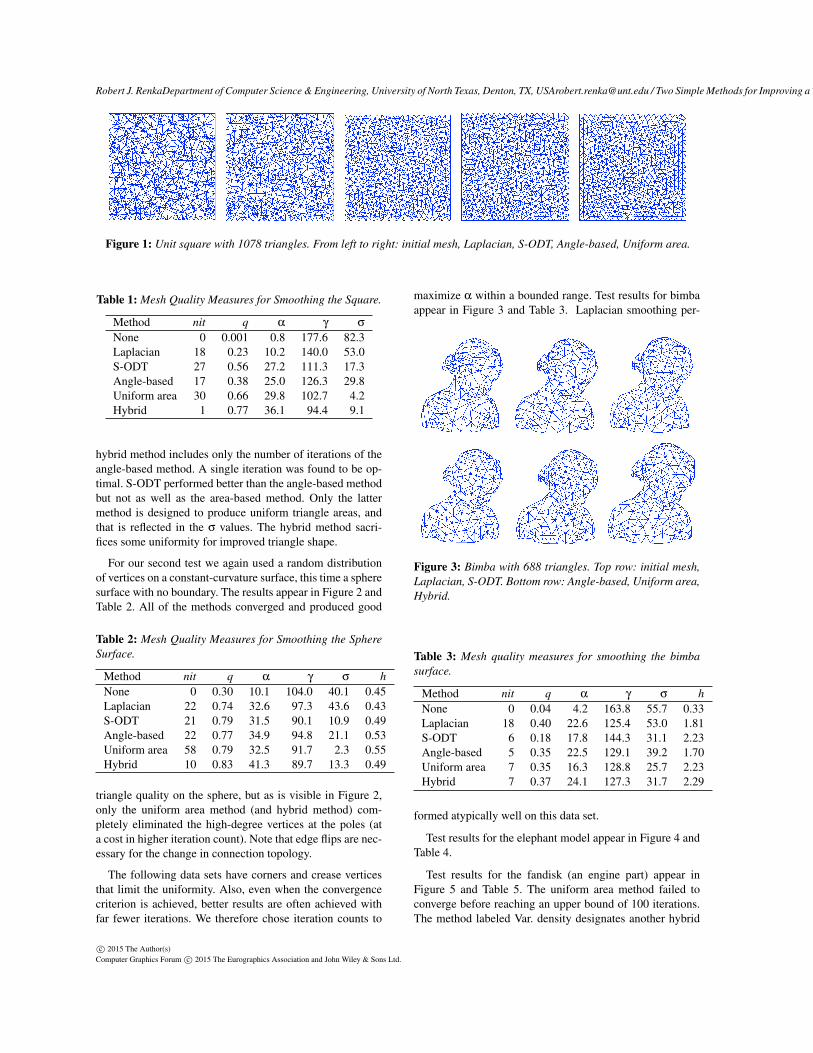
Figures and tables. Figure 1 depicts the initial mesh andthe result of applying the smoothing methods to random ver-tices in the unit square. Since the curvature is constant, thevariable density method is omitted.

The tables contain iteration counts nit and the followingtriangle mesh quality measures:

• q = 2rin/rout minimized over the triangles, where rin androut are the radii of inscribed and circumscribed circles,respectively, of a triangle.

• α is the smallest angle in degrees.• γ is the largest angle in degrees.• σ = std(r)/mean(r), where r is the set of ratios of triangle

areas to centroidal values of reciprocals of density esti-mates. The value is expressed as a percentage.

• h is the Hausdorff distance between the original and com-puted mesh expressed as a percentage of the length of thediagonal of the bounding box of the computed mesh.

The radius ratio q has values ranging from 0 correspondingto a degenerate triangle to 1 for an equilateral triangle. Thevariation σ is a measure of the discrepancy between triangleareas and their target values. The Hausdorff distances wereapproximated by a tool based on [ASE02]: MeshValmet 3.0(www.nitrc.org/projects/meshvalmet) using sample size 0.1(percentage of bounding box diagonal length). The tabulatedh values for the methods labeled None are computed dis-tances from the original meshes to themselves. These are in-versely correlated with the triangle counts. A good mesh haslarge values of q and α, and small values of γ, σ and h.

While the methods are not designed for a planar surface,the Table 1 test results for the square are a good indicationof how the methods compare in the vicinity of flat spots. TheHausdorff distance measured is omitted in this case. The uni-form area method failed to converge and was terminated byan upper bound of 30 iterations. The iteration count for the



Figure 1: Unit square with 1078 triangles. From left to right: initial mesh, Laplacian, S-ODT, Angle-based, Uniform area.

Table 1: Mesh Quality Measures for Smoothing the Square.

Method nit q α γ σ

None 0 0.001 0.8 177.6 82.3Laplacian 18 0.23 10.2 140.0 53.0S-ODT 27 0.56 27.2 111.3 17.3Angle-based 17 0.38 25.0 126.3 29.8Uniform area 30 0.66 29.8 102.7 4.2Hybrid 1 0.77 36.1 94.4 9.1

hybrid method includes only the number of iterations of theangle-based method. A single iteration was found to be op-timal. S-ODT performed better than the angle-based methodbut not as well as the area-based method. Only the lattermethod is designed to produce uniform triangle areas, andthat is reflected in the σ values. The hybrid method sacri-fices some uniformity for improved triangle shape.

For our second test we again used a random distributionof vertices on a constant-curvature surface, this time a spheresurface with no boundary. The results appear in Figure 2 andTable 2. All of the methods converged and produced good

Table 2: Mesh Quality Measures for Smoothing the SphereSurface.

Method nit q α γ σ hNone 0 0.30 10.1 104.0 40.1 0.45Laplacian 22 0.74 32.6 97.3 43.6 0.43S-ODT 21 0.79 31.5 90.1 10.9 0.49Angle-based 22 0.77 34.9 94.8 21.1 0.53Uniform area 58 0.79 32.5 91.7 2.3 0.55Hybrid 10 0.83 41.3 89.7 13.3 0.49

triangle quality on the sphere, but as is visible in Figure 2,only the uniform area method (and hybrid method) com-pletely eliminated the high-degree vertices at the poles (ata cost in higher iteration count). Note that edge flips are nec-essary for the change in connection topology.

The following data sets have corners and crease verticesthat limit the uniformity. Also, even when the convergencecriterion is achieved, better results are often achieved withfar fewer iterations. We therefore chose iteration counts to

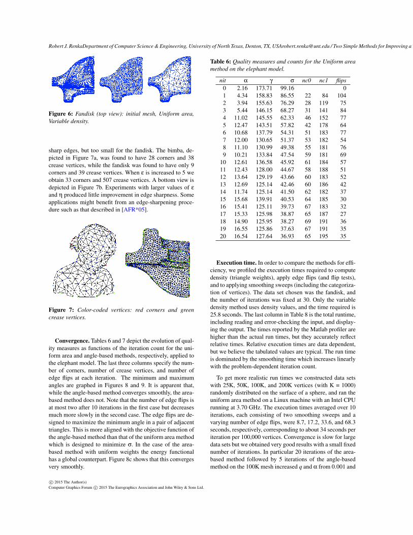
maximize α within a bounded range. Test results for bimbaappear in Figure 3 and Table 3. Laplacian smoothing per-

Figure 3: Bimba with 688 triangles. Top row: initial mesh,Laplacian, S-ODT. Bottom row: Angle-based, Uniform area,Hybrid.

Table 3: Mesh quality measures for smoothing the bimbasurface.


formed atypically well on this data set.

Test results for the elephant model appear in Figure 4 andTable 4.

Test results for the fandisk (an engine part) appear inFigure 5 and Table 5. The uniform area method failed toconverge before reaching an upper bound of 100 iterations.The method labeled Var. density designates another hybrid



Figure 2: Sphere with 840 triangles. From left to right: initial mesh, Laplacian, S-ODT, Angle-based, Uniform area.

Figure 4: Elephant with 2680 triangles. Top row: initialmesh, Laplacian, S-ODT. Bottom row: Angle-based, Uni-form area, Hybrid.

Table 4: Mesh quality measures for smoothing the elephantmodel.


method in which the angle-based method was run on the out-put from the area-based method with triangle weights com-puted from vertex curvature estimates (with a lower bound of10−5 on curvature). In both cases the iteration counts werechosen to maximize α: 89 iterations of the area-based meth-ods, resulting in α = 17.4 and σ = 14.3, followed by 5 iter-ations of the angle-based method, resulting in the tabulatedvalues. The alternative method in which density is based onestimated local feature size gave α = 11.9 and σ = 13.8 after

95 iterations. Five iterations of the angle-based method ap-plied to the output then resulted in q = 0.50, α = 21.3, andγ = 117.2.

Figure 5: Fandisk with 6094 triangles. Top row: initialmesh, Laplacian, S-ODT. Bottom row: Angle-based, Uni-form area, Variable density.

Table 5: Mesh quality measures for smoothing the fandisk.

Method nit q α γ σ hNone 0 0.00 0.0 180.0 217.4 0.11Laplacian 20 0.23 14.3 138.5 167.3 1.66S-ODT 93 0.60 22.0 107.5 19.8 1.56Angle-based 92 0.54 24.3 113.2 50.5 1.46Uniform area 100 0.61 21.5 103.7 6.4 1.69Hybrid 32 0.70 32.2 101.4 16.7 1.72Var. density 94 0.56 26.1 112.5 156.9 1.45

As is apparent in the test results, the variable densitymethod is not as effective as the hybrid uniform methodin terms of triangle quality, but it places the vertices wherethey are needed and produces well-shaped triangles with asmoothly graded mesh as shown in Figure 5 and Figure 6which depicts the same surface from a different perspective.It is apparent that sharp edges are not well-preserved in thisdata set.

Recall that we used ε = 2 and η = 2 in the vertex cat-egorization scheme. These values appear to be appropriatefor surfaces such as the bimba and elephant, which have no



Figure 6: Fandisk (top view): initial mesh, Uniform area,Variable density.

sharp edges, but too small for the fandisk. The bimba, de-picted in Figure 7a, was found to have 28 corners and 38crease vertices, while the fandisk was found to have only 9corners and 39 crease vertices. When ε is increased to 5 weobtain 33 corners and 507 crease vertices. A bottom view isdepicted in Figure 7b. Experiments with larger values of ε

and η produced little improvement in edge sharpness. Someapplications might benefit from an edge-sharpening proce-dure such as that described in [AFR*05].

Figure 7: Color-coded vertices: red corners and greencrease vertices.

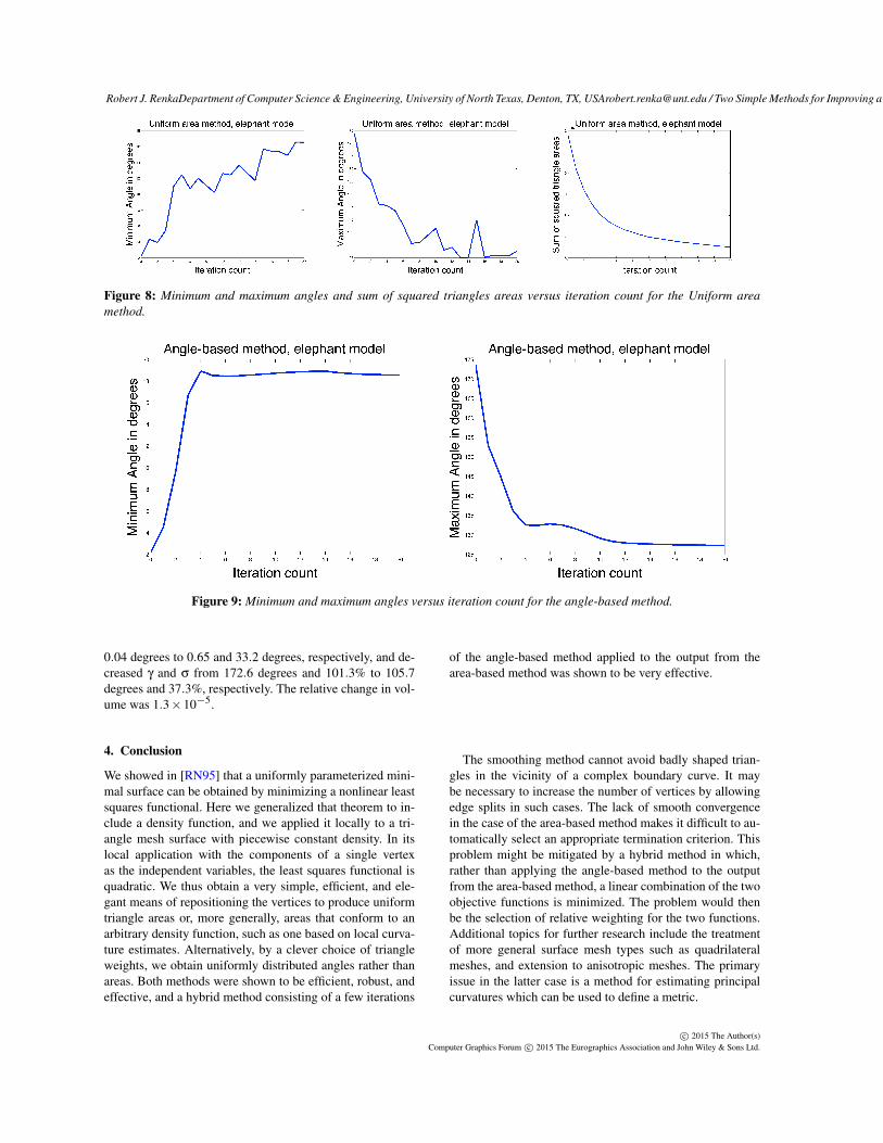
Convergence. Tables 6 and 7 depict the evolution of qual-ity measures as functions of the iteration count for the uni-form area and angle-based methods, respectively, applied tothe elephant model. The last three columns specify the num-ber of corners, number of crease vertices, and number ofedge flips at each iteration. The minimum and maximumangles are graphed in Figures 8 and 9. It is apparent that,while the angle-based method converges smoothly, the area-based method does not. Note that the number of edge flips isat most two after 10 iterations in the first case but decreasesmuch more slowly in the second case. The edge flips are de-signed to maximize the minimum angle in a pair of adjacenttriangles. This is more aligned with the objective function ofthe angle-based method than that of the uniform area methodwhich is designed to minimize σ. In the case of the area-based method with uniform weights the energy functionalhas a global counterpart. Figure 8c shows that this convergesvery smoothly.

Table 6: Quality measures and counts for the Uniform areamethod on the elephant model.

nit α γ σ nc0 nc1 flips0 2.16 173.71 99.16 01 4.34 158.83 86.55 22 84 1042 3.94 155.63 76.29 28 119 753 5.44 146.15 68.27 31 141 844 11.02 145.55 62.33 46 152 775 12.47 143.51 57.82 42 178 646 10.68 137.79 54.31 51 183 777 12.00 130.65 51.37 53 182 548 11.10 130.99 49.38 55 181 769 10.21 133.84 47.54 59 181 69

10 12.61 136.58 45.92 61 184 5711 12.43 128.00 44.67 58 188 5112 13.64 129.19 43.66 60 183 5213 12.69 125.14 42.46 60 186 4214 11.74 125.14 41.50 62 182 3715 15.68 139.91 40.53 64 185 3016 15.41 125.11 39.73 67 183 3217 15.33 125.98 38.87 65 187 2718 14.90 125.95 38.27 69 191 3619 16.55 125.86 37.63 67 191 3520 16.54 127.64 36.93 65 195 35

Execution time. In order to compare the methods for effi-ciency, we profiled the execution times required to computedensity (triangle weights), apply edge flips (and flip tests),and to applying smoothing sweeps (including the categoriza-tion of vertices). The data set chosen was the fandisk, andthe number of iterations was fixed at 30. Only the variabledensity method uses density values, and the time required is25.8 seconds. The last column in Table 8 is the total runtime,including reading and error-checking the input, and display-ing the output. The times reported by the Matlab profiler arehigher than the actual run times, but they accurately reflectrelative times. Relative execution times are data dependent,but we believe the tabulated values are typical. The run timeis dominated by the smoothing time which increases linearlywith the problem-dependent iteration count.

To get more realistic run times we constructed data setswith 25K, 50K, 100K, and 200K vertices (with K = 1000)randomly distributed on the surface of a sphere, and ran theuniform area method on a Linux machine with an Intel CPUrunning at 3.70 GHz. The execution times averaged over 10iterations, each consisting of two smoothing sweeps and avarying number of edge flips, were 8.7, 17.2, 33.6, and 68.3seconds, respectively, corresponding to about 34 seconds periteration per 100,000 vertices. Convergence is slow for largedata sets but we obtained very good results with a small fixednumber of iterations. In particular 20 iterations of the area-based method followed by 5 iterations of the angle-basedmethod on the 100K mesh increased q and α from 0.001 and



Figure 8: Minimum and maximum angles and sum of squared triangles areas versus iteration count for the Uniform areamethod.

Figure 9: Minimum and maximum angles versus iteration count for the angle-based method.

0.04 degrees to 0.65 and 33.2 degrees, respectively, and de-creased γ and σ from 172.6 degrees and 101.3% to 105.7degrees and 37.3%, respectively. The relative change in vol-ume was 1.3×10−5.

4. Conclusion

We showed in [RN95] that a uniformly parameterized mini-mal surface can be obtained by minimizing a nonlinear leastsquares functional. Here we generalized that theorem to in-clude a density function, and we applied it locally to a tri-angle mesh surface with piecewise constant density. In itslocal application with the components of a single vertexas the independent variables, the least squares functional isquadratic. We thus obtain a very simple, efficient, and ele-gant means of repositioning the vertices to produce uniformtriangle areas or, more generally, areas that conform to anarbitrary density function, such as one based on local curva-ture estimates. Alternatively, by a clever choice of triangleweights, we obtain uniformly distributed angles rather thanareas. Both methods were shown to be efficient, robust, andeffective, and a hybrid method consisting of a few iterations

of the angle-based method applied to the output from thearea-based method was shown to be very effective.

The smoothing method cannot avoid badly shaped trian-gles in the vicinity of a complex boundary curve. It maybe necessary to increase the number of vertices by allowingedge splits in such cases. The lack of smooth convergencein the case of the area-based method makes it difficult to au-tomatically select an appropriate termination criterion. Thisproblem might be mitigated by a hybrid method in which,rather than applying the angle-based method to the outputfrom the area-based method, a linear combination of the twoobjective functions is minimized. The problem would thenbe the selection of relative weighting for the two functions.Additional topics for further research include the treatmentof more general surface mesh types such as quadrilateralmeshes, and extension to anisotropic meshes. The primaryissue in the latter case is a method for estimating principalcurvatures which can be used to define a metric.



Table 7: Quality measures and counts for the Angle-basedmethod on the elephant model.

nit α γ σ nc0 nc1 flips0 2.16 173.71 99.16 01 4.47 152.99 88.76 21 81 732 9.66 145.03 80.97 25 103 293 16.73 136.12 74.93 30 124 304 18.93 132.53 70.39 36 136 175 18.51 132.43 66.91 45 152 116 18.48 132.82 64.39 49 158 147 18.49 132.48 62.67 51 158 118 18.57 131.60 61.57 50 158 59 18.65 130.40 60.88 49 159 11

10 18.73 129.07 60.35 50 164 211 18.81 128.28 59.96 54 157 212 18.86 127.93 59.69 53 160 013 18.91 127.75 59.51 56 160 214 18.93 127.63 59.36 56 160 115 18.79 127.55 59.24 55 159 016 18.70 127.48 59.14 56 159 217 18.64 127.41 59.04 54 158 018 18.60 127.35 58.97 54 158 019 18.58 127.30 58.91 54 159 020 18.57 127.25 58.85 54 159 1

Table 8: Execution times for 30 iterations on the fandisk.

Method edge flips smoothing totalLaplacian 25.3 87.0 119.1S-ODT 25.9 153.5 186.5Angle-based 25.8 128.6 161.4Uniform area 27.5 121.5 156.3Variable density 28.6 122.6 186.9

Acknowledgments

The author is grateful to the Associate editor and refereesfor numerous suggestions that improved the exposition ofthis paper.

Appendix A. Proof of Theorem 1

A theorem similar to the following appears in [GYH13].

Theorem 1 Vertex displacement in the tangent plane definedby Equation (1) preserves the volume bounded by the surface(and a cone connecting the boundary, if any, to the origin).

Proof The contribution to the volume from the star of v0 isthe sum of signed tetrahedron volumes

n

∑k=1

16〈vk×vk+1,v0〉.

The unnormalized vector defining the tangent plane at v0 is

n =n

∑k=1

(vk−v0)× (vk+1−v0)

=n

∑k=1

(vk×vk+1)+n

∑k=1

(vk+1−vk)×v0

=n

∑k=1

(vk×vk+1)

since ∑nk=1(vk+1− vk) = 0. Consider displacement from v0

to v, where v−v0 is orthogonal to n so thatn

∑k=1〈vk×vk+1,v〉=

n

∑k=1〈vk×vk+1,v0〉.

Scaling this equation by 1/6, we see that the sum of tetrahe-dron volumes is not altered by the displacement.

Appendix B. Proof of Theorem 2

The following theorem appears in Section 2.2.

Theorem 2 A is positive definite.

Proof A straightforward exercise shows that A has positiveeigenvalues if and only if its determinant ac−b2 is positive.Define u and v in Rn by

uk =√

wk〈ek,e2〉 and vk =√

wk〈ek,e1〉.

Then a = ‖u‖2,b = 〈u,v〉, and c = ‖v‖2. Hence, by theCauchy-Schwarz inequality,

ac−b2 = ‖u‖2‖v‖2−〈u,v〉2 ≥ 0

with equality if and only if u and v are linearly dependent,implying that for some α, 〈ek,e2〉 = α〈ek,e1〉; i.e., ek is or-thogonal to e2−αe1 for all k, and hence v0 and all its neigh-bors are coplanar. However, the only plane than can containall the triangles is the tangent plane whose normal is orthog-onal to e2−αe1. Therefore u and v are linearly independentand ac−b2 > 0.

Appendix C. Proof of Theorem 3

The following theorem from Section 2.3 shows that criti-cal points of ψ (Equation (5)) are uniformly parameterized.

Theorem 3 If f is a critical point of ψ then ρ‖ f1× f2‖ isconstant.

Proof Denoting by h an element of the linear space of varia-tions in f that preserve boundary values, the Fréchet deriva-tive of ψ at f is

ψ′( f )h =

ZΩ

ρ〈 f1×h2 +h1× f2, f1× f2〉

=Z

Ω

ρ(〈h1, f2× f1× f2〉+ 〈h2, f1× f2× f1〉)

= −Z

Ω

〈h,D1[ρ( f2× f1× f2)]

+D2[ρ( f1× f2× f1)]〉= 〈h,−D1[ρ( f2× f1× f2)]

−D2[ρ( f1× f2× f1)]〉L2(Ω,R3),

where D1 and D2 denote first partial derivative operators. A



critical point of ψ is thus characterized by a zero of the L2

gradient

∇ψ( f ) = −D1[ρ( f2× f1× f2)]−D2[ρ( f1× f2× f1)]

= −D1[ f2×ρ( f1× f2)]−D2[ f1×ρ( f2× f1)]

= −D1( f2)×ρ( f1× f2)− f2×D1[ρ( f1× f2)]

+D2( f1)×ρ( f1× f2)+ f1×D2[ρ( f1× f2)]

= − f2×D1[ρ( f1× f2)]+ f1×D2[ρ( f1× f2)],

where the last equation follows from the assumption of con-tinuous mixed second partial derivatives. Hence

D1[ρ‖ f1× f2‖] =〈ρ( f1× f2),D1[ρ( f1× f2)]〉

‖ρ( f1× f2)‖

=〈 f1× f2,D1[ρ( f1× f2)]〉

‖ f1× f2‖

=〈 f1, f2×D1[ρ( f1× f2)]〉

‖ f1× f2‖

=−〈 f1,∇ψ( f )〉‖ f1× f2‖

= 0

and

D2[ρ‖ f1× f2‖] =〈ρ( f1× f2),D2[ρ( f1× f2)]〉

‖ρ( f1× f2)‖

=〈 f1× f2,D2[ρ( f1× f2)]〉

‖ f1× f2‖

=−〈 f2, f1×D2[ρ( f1× f2)]〉

‖ f1× f2‖

=−〈 f2,∇ψ( f )〉‖ f1× f2‖

= 0

References

[ABK98] Amenta N., Bern M., Kamvysselis M.: A new Voronoi-based surface reconstruction algorithm. In SIGGRAPH ’98 Pro-ceedings of the 25th Annual Conference on Computer Graphicsand Interactive Techniques (1998), pp. 415–421.

[ASE02] Aspert N., Santa-Cruz D., Ebrahimi T.: MESH: measur-ing errors between surfaces using the Hausdorff distance, In Pro-ceedings of the IEEE International Conference on Multimediaand Expo (2002), pp. 705–708.

[AFR*05] Attene M., Falcidieno B., Rossignac J., SpagnuoloM.: Sharpen&Bend: recovering curved sharp edges in trianglemeshes produced by feature-insensitive sampling. IEEE Trans.Vis. Comput. Graph. 11, 2 (Mar-Apr 2005), 181–192.

[CHE04] Chen L.: Mesh smoothing schemes based on optimalDelaunay triangulations. In Proceedings of the Thirteenth Inter-national Meshing Roundtable (2004), pp. 109–120.

[CDS13] Cheng S.-W., Dey T.K., Shewchuk J.R.: Delaunay MeshGeneration. Chapman & Hall, 2013.

[CR84] Cline A.K., Renka R.J.: A storage-efficient method forconstruction of a Thiessen triangulation. Rocky Mountain Jour-nal of Mathematics 14, 1 (1984), 119–139.

[DMS*99] Desbrun M., Meyer M., Schröder P., Barr A.H.: Im-plicit Fairing of Irregular Meshes using Diffusion and Curvature

Flow. In SIGGRAPH ’99 Proceedings the 26th annual confer-ence on Computer graphics and interactive techniques (1999),pp. 317–324.

[DR10] Dey T.K., Ray T.: Polygonal surface remeshing with De-launay refinement. Engineering with Computers 26 (2010), 289–301.

[DZM07] Dyer R., Zhang H., Möller T.: Delaunay mesh construc-tion. In Proceedings of the Fifth Eurographics Symposium on Ge-ometry Processing (2007), pp. 273–282.

[FIE88] Field D.: Laplacian smoothing and Delaunay triangu-lations. Communications in Applied Numerical Methods 4, 6(1988), 709–712.

[GYH13] Gao Z., Yu Z., Holst M.: Feature-preserving surfacemesh smoothing via suboptimal Delaunay triangulation. Graphi-cal Models 75, 1 (2013), 23–38.

[HS13] He L., Schaefer S.: Mesh denoising via L0 minimization.ACM Trans. Graph. 32, 4 (2013), 1–8.

[LAW72] Lawson C.L.: Transforming triangulations. DiscreteMathematics 3, 4 (1972), 365–372.

[LL03] Lee Y.K., Lee C.K.: A new indirect anisotropic quadrilat-eral mesh generation scheme with enhanced local mesh smooth-ing procedures. Int. J. Num. Meth. Eng. 58 (2003), 277–300.

[PSK*02] Page D.L., Sun Y., Koschan A.F., Paik J., Abidi M.A.:Normal vector voting: crease detection and curvature estimationon large, noisy meshes. Graphical Models 64, 3-4 (2002), 199–229.

[RN95] Renka R.J., Neuberger J.W.: Minimal surfaces andSobolev gradients. SIAM J. Sci. Comput. 16 (1995), 1412–1427.

[REN14] Renka R.J.: A trust region method for constructingtriangle-mesh approximations of parametric minimal surfaces.Appl. Numer. Math. 76C (2014), 93–100.

[REN15] Renka R.J.: Mesh improvement by minimizing aweighted sum of squared element volumes. Int. J. Num. Meth.Eng. 101 (2015), 870–886.

[SG02] Surazhsky V., Gotsman C.: High quality compatible trian-gulations, In Proceedings of the Eleventh International MeshingRoundtable (2002), pp. 183–192.

[SG03] Surazhsky V., Gotsman C.: Explicit surface remeshing, InProceedings of the 2003 Eurographics/ACM SIGGRAPH sympo-sium on Geometry processing (2003) pp. 20–30.

[WY11] Wang J., Yu Z.: Quality mesh smoothing via local surfacefitting and optimum projection. Graphical Models 73 (2011),127–139.

[XN06] Xu H., Newman T.S.: An angle-based optimization ap-proach for 2D finite element mesh smoothing. Finite Elements inAnalysis and Design 42 (2006), 1150–1164.

[XHG*12] Xu Y., Hu R., Gotsman C., Liu L.: Blue noisesampling of surfaces. Comput. Graph. 36,4 (2012), 232–240.doi:10.1016/j.cag.2012.02.005.

[ZBX09] Zhang Y., Bajaj C., Xu, G.: Surface smoothing and qual-ity improvement of quadrilateral/hexahedral meshes with geo-metric flow. Commun. Numer. Meth. Eng. 25,1 (2009), 1–18.

[ZS00] Zhou T., Shimada K.: An angle-based approach to two-dimensional mesh smoothing. In Proceedings of the Ninth Inter-national Meshing Roundtable (2000), pp. 373–384.


two simple methods for improving a triangle mesh surface

Documents