Two-periodic Aztec diamond

Arno Kuijlaars (KU Leuven)

joint work with

Maurice Duits (KTH Stockholm)

Optimal and Random Point Configurations

ICERM, Providence, RI, U.S.A., 27 February 2018

Outline

1. Aztec diamond

2. The model and main result

3. Non-intersecting paths

4. Matrix Valued Orthogonal Polynomials (MVOP)

5. Analysis of RH problem

6. Saddle point analysis

7. Periodic tilings of a hexagon

1. Aztec diamond

Aztec diamond

West

North

South

East

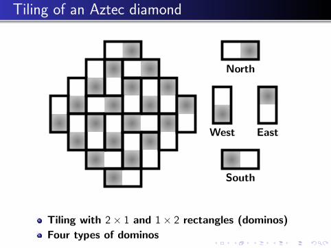
Tiling of an Aztec diamond

West

North

South

East

Tiling with 2× 1 and 1× 2 rectangles (dominos)

Four types of dominos

Large random tiling

Deterministicpattern nearcornersSolid regionorFrozen region

Disorder in themiddleLiquid region

Boundary curveArctic circle

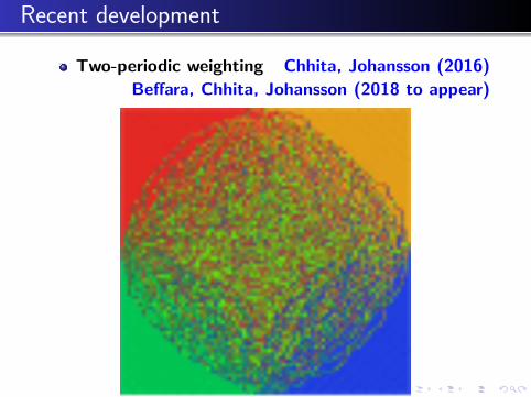
Recent development

Two-periodic weighting Chhita, Johansson (2016)

Beffara, Chhita, Johansson (2018 to appear)

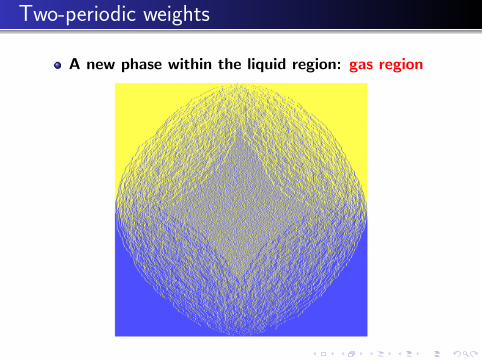
Two-periodic weights

A new phase within the liquid region: gas region

Phase diagram

solid

solid

solid

solid

gas

liquid

2. The model and main result

Two periodic weights

b b

a a a a

a a a a

b b

b b

a

a

b

b

b

b

Aztec diamond of size 2N

Weight w(T )of a tiling T isthe product ofthe weights ofdominos

Partition function

ZN =∑T

w(T )

Probability for T

Prob(T ) =w(T )

ZN

Equivalent weights

β

α α

α α

β

β

α

β

β

α = a2 and β = b2

North and Eastdominos haveweight 1

Without loss ofgenerality

αβ = 1

and α ≥ 1

Since North dominos have weight 1, we can transferthe weights to non-intersecting paths.

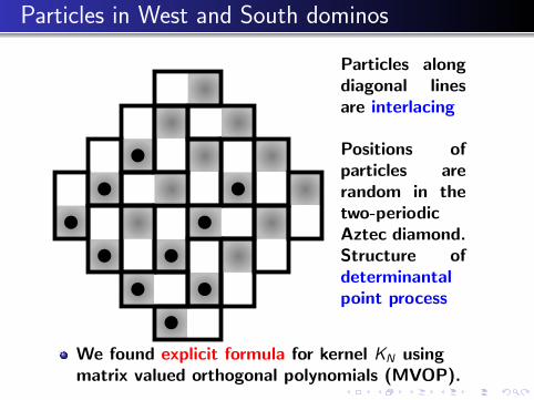
Particles in West and South dominos

Particles alongdiagonal linesare interlacing

Positions ofparticles arerandom in thetwo-periodicAztec diamond.Structure ofdeterminantalpoint process

We found explicit formula for kernel KN usingmatrix valued orthogonal polynomials (MVOP).

Coordinates

m runs

from 0 to 2N

n runs

from 0 to 2N − 1

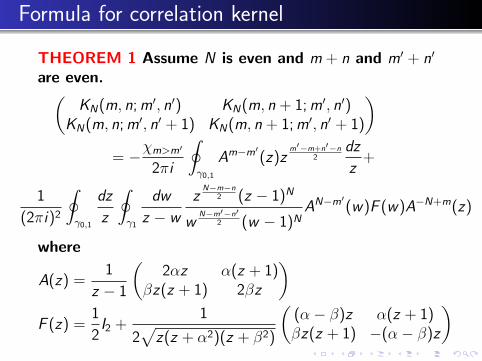
Formula for correlation kernel

THEOREM 1 Assume N is even and m + n and m′ + n′

are even.(KN(m, n;m′, n′) KN(m, n + 1;m′, n′)

KN(m, n;m′, n′ + 1) KN(m, n + 1;m′, n′ + 1)

)= −χm>m′

2πi

∮γ0,1

Am−m′(z)zm′−m+n′−n

2dz

z+

1

(2πi)2

∮γ0,1

dz

z

∮γ1

dw

z − w

zN−m−n

2 (z − 1)N

wN−m′−n′

2 (w − 1)NAN−m′(w)F (w)A−N+m(z)

where

A(z) =1

z − 1

(2αz α(z + 1)

βz(z + 1) 2βz

)F (z) =

1

2I2 +

1

2√

z(z + α2)(z + β2)

((α− β)z α(z + 1)βz(z + 1) −(α− β)z

)

3. Non-intersecting paths

Non-intersecting paths

Line segments onWest, East and South

dominos

North

West East

South

Double Aztec diamond

2N particles

along each

diagonal line

Non-intersecting paths on a graph

Paths are transformed to fit on a graph

0 0.5 1 1.5 2 2.5 3 3.5 4

-2

-1

0

1

2

3

4

5

6

Weights on the graph

0 0.5 1 1.5 2 2.5 3 3.5 4

-2

-1

0

1

2

3

4

5

6

αα

αα

αα

αα

αα

αα

αα

αα

αα

αα

αα

αα

αα

αα

αα

αα

αα

αα

αα

αα

ββ

ββ

ββ

ββ

ββ

ββ

ββ

ββ

ββ

ββ

ββ

ββ

ββ

ββ

ββ

ββ

ββ

ββ

ββ

ββ

Weights on non-intersecting paths

Any tiling of double Aztec diamond is equivalent tosystem (P0, . . . ,P2N−1) of 2N non-intersecting paths

Pj is path on the graph from (0, j) to (2N , j),

Pi is vertex disjoint from Pj if i 6= j .

Transitions and LGV theorem

There are 2N + 1 levels, 0, 1, . . . , 2N.

Transition from level m to level m′ > m

Tm,m′(x , y) =∑

P:(m,x)→(m′,y)

w(P), x , y ∈ Z

Lindstrom-Gessel-Viennot theorem

Probability that paths at level m are at positionsx(m)0 < x

(m)1 < · · · < x

(m)2N−1:

1

ZNdet[T0,m(i , x

(m)k )

]2N−1i ,k=0

· det[Tm,2N(x

(m)k , j)

]2N−1k,j=0

Lindstrom (1973)Gessel-Viennot (1985)

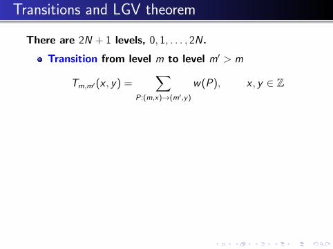
Transitions and LGV theorem

There are 2N + 1 levels, 0, 1, . . . , 2N.

Transition from level m to level m′ > m

Tm,m′(x , y) =∑

P:(m,x)→(m′,y)

w(P), x , y ∈ Z

Lindstrom-Gessel-Viennot theorem

Probability that paths at level m are at positionsx(m)0 < x

(m)1 < · · · < x

(m)2N−1:

1

ZNdet[T0,m(i , x

(m)k )

]2N−1i ,k=0

· det[Tm,2N(x

(m)k , j)

]2N−1k,j=0

Lindstrom (1973)Gessel-Viennot (1985)

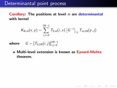
Determinantal point process

Corollary: The positions at level m are determinantalwith kernel

KN,m(x , y) =2N−1∑i ,j=0

T0,m(i , x)[G−t

]i ,jTm,2N(y , j)

where G = [T0,2N(i , j)]2N−1i ,j=0

Multi-level extension is known as Eynard-Mehtatheorem.

Block Toeplitz matrices

In our case: Transition matrices are 2 periodic

T (x + 2, y + 2) = T (x , y)

Block Toeplitz matrices, infinite in both directions,

with block symbol A(z) =∞∑

j=−∞

Bjzj

if T =

. . . . . . . . .

. . . B0 B1. . .

. . . B−1 B0 B1. . .

. . . B−1 B0. . .

. . . . . . . . .

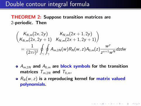
Double contour integral formula

THEOREM 2: Suppose transition matrices are2-periodic. Then(

KN,m(2x , 2y) KN,m(2x + 1, 2y)KN,m(2x , 2y + 1) KN,m(2x + 1, 2y + 1)

)=

1

(2πi)2

∮γ

∮γ

Am,2N(w)RN(w , z)A0,m(z)w y

zx+1wNdzdw

Am,2N and A0,m are block symbols for the transitionmatrices Tm,2N and T0,m.

RN(w , z) is a reproducing kernel for matrix valuedpolynomials.

4. Matrix Valued OrthogonalPolynomials (MVOP)

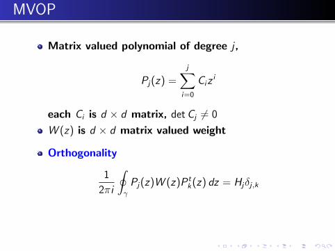
MVOP

Matrix valued polynomial of degree j ,

Pj(z) =

j∑i=0

Cizi

each Ci is d × d matrix, detCj 6= 0

W (z) is d × d matrix valued weight

Orthogonality

1

2πi

∮γ

Pj(z)W (z)P tk(z) dz = Hjδj ,k

Reproducing kernel

RN(w , z) =N−1∑j=0

P tj (w)H−1j Pj(z)

is reproducing kernel for matrix polynomials of degree≤ N − 1

If Q has degree ≤ N − 1, then

1

2πi

∮γ

Q(w)W (w)RN(w , z)dw = Q(z)

There is a Christoffel-Darboux formula for RN and aRiemann Hilbert problem

Riemann-Hilbert problem

Y : C \ γ → C2d×2d satisfies

Y is analytic,

Y+ = Y−

(Id W0d Id

)on γ,

Y (z) = (I2d + O(z−1))

(zN Id 0d

0d z−N Id

)as z →∞.

Grunbaum, de la Iglesia, Martınez-Finkelshtein (2011)

Solution of RH problem

Unique solution (provided PN uniquely exists) is

Y (z) =

PN(z)1

2πi

∮γ

PN(s)W (s)

s − zds

QN−1(z)1

2πi

∮γ

QN−1(s)W (s)

s − zds

where PN is monic MVOP of degree N andQN−1 = −H−1N−1PN−1 has degree N − 1

Christoffel Darboux formula

RN(w , z) =1

z − w

(0d Id

)Y −1(w)Y (z)

(Id0d

)Delvaux (2010)

Solution of RH problem

Unique solution (provided PN uniquely exists) is

Y (z) =

PN(z)1

2πi

∮γ

PN(s)W (s)

s − zds

QN−1(z)1

2πi

∮γ

QN−1(s)W (s)

s − zds

where PN is monic MVOP of degree N andQN−1 = −H−1N−1PN−1 has degree N − 1

Christoffel Darboux formula

RN(w , z) =1

z − w

(0d Id

)Y −1(w)Y (z)

(Id0d

)Delvaux (2010)

Our case of interest

Weight matrix in special case of two periodic Aztecdiamond is W N(z), with

W (z) =1

(z − 1)2

((z + 1)2 + 4α2z 2α(α + β)(z + 1)

2β(α + β)z(z + 1) (z + 1)2 + 4β2z

)No symmetry in W . Existence and uniqueness ofMVOP are not immediate.

Scalar valued analogue

Weight(z+1z−1

)Non circle around z = 1 and OPs are

Jacobi polynomials P(−N,N)j (z) with nonstandard

parameters

Our case of interest

Weight matrix in special case of two periodic Aztecdiamond is W N(z), with

W (z) =1

(z − 1)2

((z + 1)2 + 4α2z 2α(α + β)(z + 1)

2β(α + β)z(z + 1) (z + 1)2 + 4β2z

)No symmetry in W . Existence and uniqueness ofMVOP are not immediate.

Scalar valued analogue

Weight(z+1z−1

)Non circle around z = 1 and OPs are

Jacobi polynomials P(−N,N)j (z) with nonstandard

parameters

5. Analysis of RH problem

Surprise

Steepest descent analysis of RH problem leads toexplicit formula

RH problem is solved in terms of contour integrals.

For example: MVOP is

PN(z) = (z − 1)NW N/2∞ W−N/2(z), if N is even.

It leads to proof of THEOREM 1

Surprise

Steepest descent analysis of RH problem leads toexplicit formula

RH problem is solved in terms of contour integrals.

For example: MVOP is

PN(z) = (z − 1)NW N/2∞ W−N/2(z), if N is even.

It leads to proof of THEOREM 1

6. Saddle point analysis

Asymptotic analysis

Saddle point analysis on the double contour integral

1

(2πi)2

∮γ0,1

dz

z

∮γ1

dw

z − w

zN−2x

2 (z − 1)N

wN−2y

2 (w − 1)NAN−m(w)F (w)A−N+m(z)

when N →∞m, x , y scale with N in such a way that

m ≈ (1 + ξ1)N , x , y ≈ (1 + ξ1+ξ22

)N

Saddle points are critical points of

2 log(z − 1)− (1 + ξ2) log z + ξ1 log λ(z)

where λ(z) is an eigenvalue of W (z) =A2(z)

z.

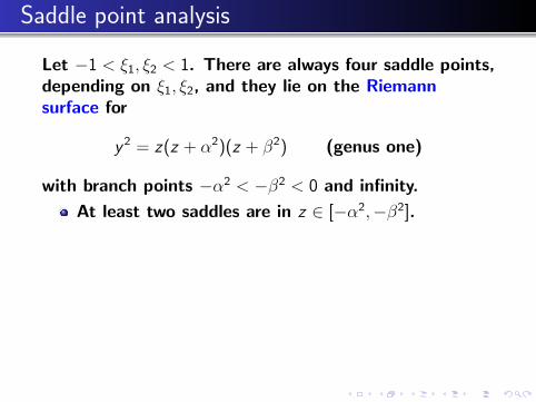
Saddle point analysis

Let −1 < ξ1, ξ2 < 1. There are always four saddle points,depending on ξ1, ξ2, and they lie on the Riemannsurface for

y 2 = z(z + α2)(z + β2) (genus one)

with branch points −α2 < −β2 < 0 and infinity.

At least two saddles are in z ∈ [−α2,−β2].

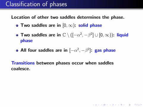
Classification of phases

Location of other two saddles determines the phase.

Two saddles are in [0,∞): solid phase

Two saddles are in C \ ([−α2,−β2] ∪ [0,∞)): liquidphase

All four saddles are in [−α2,−β2]: gas phase

Transitions between phases occur when saddlescoalesce.

Phase diagram

solid

solid

solid

solid

gas

liquid

liquid

liquid

liquid

7. Periodic tilings of a hexagon

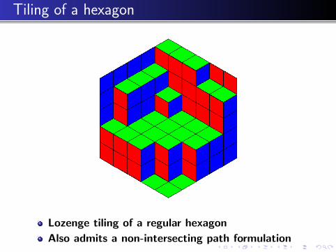
Tiling of a hexagon

Lozenge tiling of a regular hexagon

Also admits a non-intersecting path formulation

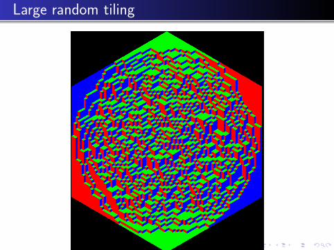
Large random tiling

Two periodic tiling of a hexagon

Ongoing work withCharlier, Duits, and Lenells

Thanks

Thank you for your attention